| Issue |
A&A
Volume 651, July 2021
|
|
|---|---|---|
| Article Number | A96 | |
| Number of page(s) | 27 | |
| Section | Stellar structure and evolution | |
| DOI | https://doi.org/10.1051/0004-6361/202040195 | |
| Published online | 23 July 2021 | |
Constraining the overcontact phase in massive binary evolution
I. Mixing in V382 Cyg, VFTS 352, and OGLE SMC-SC10 108086
1
European Southern Observatory, Alonso de Cordova 3107, Vitacura, Casilla 19001, Santiago de Chile, Chile
e-mail: This email address is being protected from spambots. You need JavaScript enabled to view it.
2
Institute of Astrophysics, KU Leuven, Celestijnenlaan 200 D, 3001 Leuven, Belgium
3
Escola de Ciências e Tecnologia, Universidade Federal do Rio Grande do Norte, Natal, RN 59072-970, Brazil
4
Departamento de Física, Universidade do Estado do Rio Grande do Norte, Mossoró, RN 59610-210, Brazil
5
Astronomical Institute Anton Pannekoek, Amsterdam University, Science Park 904, 1098 XH Amsterdam, The Netherlands
6
Max-Planck-Institut für Astrophysik, Karl-Schwarzschild-Straße 1, 85740 Garching bei München, Germany
7
Harvard-Smithsonian Center for Astrophysics, Harvard University, 60 Garden St, Cambridge, MA 02138, USA
8
School of Astronomy & Space Science, University of the Chinese Academy of Sciences, Beijing 100012, PR China
9
Argelander-Institut für Astronomie, Universität Bonn, Auf dem Hügel 71, 53121 Bonn, Germany
10
Royal Observatory of Belgium, Avenue Circulaire 3, 1180 Brussel, Belgium
11
LMU München, Universitätssternwarte, Scheinerstr. 1, 81679 München, Germany
Received:
21
December
2020
Accepted:
14
April
2021
Abstract
Context. As potential progenitors of several exotic phenomena including gravitational wave sources, magnetic stars, and Be stars, close massive binary systems probe a crucial area of the parameter space in massive star evolution. Despite the importance of these systems, large uncertainties regarding the nature and efficiency of the internal mixing mechanisms still exist.
Aims. We aim to provide robust observational constraints on the internal mixing processes by spectroscopically analyzing a sample of three massive overcontact binaries at different metallicities.
Methods. Using optical phase-resolved spectroscopic data, we performed an atmosphere analysis using more traditional 1D techniques and the most recent 3D techniques. We compared and contrasted the assumptions and results of each technique and investigated how the assumptions affect the final derived atmospheric parameters.
Results. We find that in all three cases, both components of a system are highly overluminous, indicating either efficient internal mixing of helium or previous nonconservative mass transfer. However, we do not find strong evidence of the helium or CNO surface abundance changes that are usually associated with mixing. Additionally, we find that in unequal-mass systems, the measured effective temperature and luminosity of the less massive component places it very close to the more massive component on the Hertzsprung–Russell diagram. These results were obtained independently using both of the techniques mentioned above. This suggests that these measurements are robust.
Conclusions. The observed discrepancies between the temperature and the surface abundance measurements when compared to theoretical expectations indicate that additional physical mechanisms that have not been accounted for so far may be at play.
Key words: stars: massive / binaries: spectroscopic / binaries: close
© ESO 2021
1. Introduction
Through their ionizing fluxes, strong stellar winds, and powerful explosions, massive stars play a crucial role in the star formation process and drive the chemical evolution of their host galaxies (for a review, see Bresolin et al. 2008). Understanding how these massive stars form, evolve, and how they end their lives is thus of vital importance to our understanding of the universe in general. A common feature seen in massive star systems is a tendency to be found in close binary systems (e.g., Sana & Evans 2011), and this can have a large effect on the evolution of the component stars. It has been demonstrated that about 40% of all O-type stars will interact with a companion during their lifetimes (Sana et al. 2012), and about half of these interactions (∼25 % of all O-type stars) are expected to result in an overcontact configuration (e.g., Pols 1994; Wellstein et al. 2001; de Mink et al. 2007).
The overcontact phase represents a crossroad in the evolution of massive close binary systems. Depending on the nature and efficiency of the internal physical processes and on the rate of mass transfer when the system initially comes into contact, this phase can lead to various exotic astronomical objects. The overcontact phase is often short lived, evolving on the thermal or dynamical timescale, meaning that it is rather rare to observe a system during this phase. However, if the conditions are right, stable overcontact systems that evolve on the nuclear timescale can form (de Mink & Mandel 2016; Mandel & de Mink 2016; Marchant et al. 2016; Menon et al. 2020). Here we focus on these stable systems. While many factors affect the final fate of stable massive overcontact systems, one of the most important and arguably least well constrained is internal mixing. If the mixing is efficient enough, the stars may enter the chemically homogeneous evolution regime (CHE; Maeder 1987), which has several interesting evolutionary implications, including the formation of long gamma-ray bursts (Woosley & Heger 2006; Yoon et al. 2006) and the production of ionizing photons in low-metallicity star-forming regions (Szécsi et al. 2015). Instead of expanding as they evolve, stars evolving through the CHE pathway may shrink. This pathway has been proposed as a way to form gravitational wave progenitors (de Mink & Mandel 2016; Mandel & de Mink 2016; Marchant et al. 2016; du Buisson et al. 2020; Riley et al. 2021). If mixing is less efficient, then these systems will merge, potentially forming objects such as magnetic massive stars (Schneider et al. 2019), Be stars (Shao & Li 2014), luminous blue variables (Justham et al. 2014; Smith et al. 2018), blue stragglers (Eggen & Iben 1989; Mateo et al. 1990). These internal mixing processes therefore need to be constrained to accurately model the future evolution of massive overcontact systems and consequently, their final fates. Mixing affects the internal structure and thus the stellar properties such as the temperature, radius, and luminosity. If mixing extends to the surface, then it can also affect the surface chemical abundances. By studying the temperature and surface abundances and comparing them with evolutionary models, we can constrain the degree of internal mixing during this phase (e.g., de Mink et al. 2009).
In total, ten massive O+O overcontact binaries are currently known: V382 Cyg, TU Mus, MY Cam, UW CMa, HD 64315, LSS 3074, VFTS 066, VFTS 352, BAT99 126, and OGLE SMC-SC10 108086 (Leung & Schneider 1978; Popper 1978; Hilditch et al. 2005; Penny et al. 2008; Lorenzo et al. 2014, 2017; Almeida et al. 2015; Howarth et al. 2015; Mahy et al. 2020a; Janssens et al. 2021). Of these ten systems, six are located in the Milky Way, three in the Large Magellanic Cloud (LMC henceforth), and one in the Small Magellanic Cloud (SMC henceforth). Despite its small size, this sample is fairly well distributed across the relevant parameter spaces of mass ratio, total system mass, fillout factor, period, component radii, metallicity, and multiplicity, meaning that a full analysis of the complete sample will provide some much needed insights into the mixing mechanisms during this crucial phase. The fillout factor f is a measure of the degree to which a system is overfilling its roche lobes and has several different definitions in the literature. In this study we use the definition first proposed by Mochnacki & Doughty (1972),
 (1)
(1)
where Ωn, 1 and Ωn, 2 denote the normalized potential of the surface passing through L1 and L2, respectively, and Ωn indicates the actual surface potential of the system. In this definition, an overcontact system has a fillout factor 1 < f < 2, with higher fillout factors corresponding to systems in deeper contact. A fillout factor of exactly 1 implies a contact system where both components exactly fill their roche lobes, while a fillout factor 2 implies that the system is at the limit of overflowing through the L2 Lagrangian point.
This series of papers aims to spectroscopically analyze O+O overcontact binaries to provide robust observational constraints on the internal mixing processes and to better understand the properties and evolutionary outcomes of the shortest-period massive binaries. In this pilot study, we focus on three such systems in order to present our analysis techniques and investigate any initial trends or commonalities in the sample.
The goal of this study is twofold. First, we aim to place constraints on the internal mixing processes during the overcontact phase of massive binary evolution, and second, we investigate how the results of atmosphere fitting change when spherical geometry versus a more realistic 3D geometry is considered. In Sect. 2 we discuss our sample and data reduction techniques. Section 3 details the two spectroscopic fitting techniques we used, which both rely on the same underlying atmosphere models but differ in the adopted geometry: (i) assuming spherical geometry and (ii) using a realistic 3D mesh representation of the surface. In Sect. 4 we discuss the results of the two methods, and in Sect. 5 we place our findings into an evolutionary context. In this section, we also discuss how the results of the two analysis techniques compare to each other, and we discuss systematic differences that arise. Finally, Sect. 6 summarizes our findings and discusses future prospects.
2. Sample and observations
Our sample consists of three massive overcontact systems at different metallicities. These three objects were selected not only due to data availability and wavelength coverage, but also because they each probe different areas of the parameter space. The surface geometry and temperature structure for each system is shown in Fig. 1, and each system is discussed below.
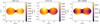 |
Fig. 1. PHOEBE II mesh model of V382 Cyg (left), VFTS 352 (center), and SMC 108086 (right). The mesh color represents the local effective temperature; lighter colors represent higher temperatures and darker colors represent lower temperatures. The systems have been inclined based on the system inclinations as given in Table 1. |
2.1. V382 Cyg
V382 Cyg is located in the Milky Way and was the first massive overcontact binary identified (Cester et al. 1978; Popper 1978). With a period of ∼1.886 days, the unequal masses of the component stars (26 + 19 M⊙) as well as an observed period increase (∼3.28 s per century) suggest that the system is undergoing conservative mass transfer from the less massive component to the more massive component at a rate of approximately 5.0 × 10⁻⁶ M⊙ yr−1 (Deǧirmenci et al. 1999; Martins et al. 2017). This system was also studied spectroscopically by Martins et al. (2017), who found that the system showed baseline CNO surface abundances. Modeling of the light curve indicates that the system has a fairly low fillout factor of 1.1, meaning that the components are only just overfilling their Roche lobes (Deǧirmenci et al. 1999; Martins et al. 2017).
Our data set for V382 Cyg consists of 89 well-phase-covered spectra collected over a two-month period using the High-Efficiency and high-Resolution Mercator Echelle Spectrograph (HERMES; Raskin et al. 2011) mounted on the Mercator Telescope in La Palma (HERMES Program 79; PI: M. Abdul-Masih). The usable wavelength range of our observations spans from ∼4000 to 9000 Å with a spectral resolution of 85 000. The data were reduced using the HERMES automatic pipeline, resulting in data with similar signal-to-noise ratios per pixel of about 50 at each epoch.
2.2. VFTS 352
VFTS 352 is located in the Tarantula region of the LMC. Its subsolar metallicity, short period (∼1.124 days), and high component masses (∼29 + 29 M⊙) make this system a good candidate for the CHE pathway. It was first discovered and characterized by Almeida et al. (2015) and was later studied spectroscopically by Abdul-Masih et al. (2019) and Mahy et al. (2020b). These studies showed that the combination of temperature and surface abundances could not be reproduced by single or binary evolutionary models, emphasizing our lack of understanding of the complex internal processes during the contact phase. With a fillout factor of 1.29 and a mass ratio of almost unity, the geometry of VFTS 352 is representative of a prototypical massive overcontact system, where a rapid phase of mass transfer has equalized the masses and the system is now thought to be in a long-lasting slow case A phase evolving on the nuclear timescale.
For this current study, we used the spectroscopic data set from Abdul-Masih et al. (2019), which consists of 8 far-UV spectra obtained with the Cosmic Origins Spectrograph (COS) on the Hubble Space Telescope (HST) under the auspices of program GO 13806 (PI: Sana) and 32 optical spectra obtained with the FLAMES-GIRAFFE spectrograph on the ESO VLT as part of the TMBM (Tarantula Massive Binary Monitoring; PI: H. Sana; ESO programs: 090.D-0323 and 092.D-0136 Almeida et al. 2017). For the purposes of this study, we used only the optical portion of the spectrum as the UV lines are much more affected by the wind parameters than the optical lines. The optical data span from ∼3950 to 4550 Å and are well phase-covered. These data were reduced using the ESO CPL GIRAFFE pipeline v.2.12.1, resulting in data with similar signal-to-noise ratios per pixel of about 150 at each epoch. Further details regarding the observational setup and data reduction can be found in Sect. 2 of Abdul-Masih et al. (2019).
2.3. SMC 108086
OGLE SMC-SC10 108086 (SMC 108086 henceforth) is located in the SMC and is the massive overcontact system with the lowest currently known metallicity. This unequal-mass system (∼17 + 14 M⊙) was photometrically characterized as a contact system by Hilditch et al. (2005), and the ephemeris and period were later updated by Pawlak et al. (2016). This system has the shortest period (∼0.883 days) and highest fillout factor (∼1.7) of all currently known massive overcontact systems, making it an interesting candidate to study the internal mixing processes during this phase.
Our data set for SMC 108086 consists of 12 evenly phased spectra collected over a six-month period (ESO program: 0103.D-0237; PI: M. Abdul-Masih) using the X-shooter multiwavelength spectrograph on the ESO VLT (Vernet et al. 2011). When the three arms are combined, the wavelength coverage spans from 3000 to 25 000 Å with spectral resolutions of 6700, 8900, and 5600 for the UVB, VIS, and NIR arms, respectively. Each of the 12 epochs consists of one nodding cycle with 1415 s exposures in UVB, 1478 s in VIS, and 1200 s in NIR. These data were reduced following the standard procedure using the ESOReflex automated reduction pipeline (Freudling et al. 2013). The resulting data at each individual epoch have similar signal-to-noise ratios per pixel of about 160 at ∼4800 Å.
2.4. Normalization
One of the three systems in our sample (VFTS 352) has been spectroscopically analyzed in a previous study, so that the data are already normalized (Abdul-Masih et al. 2019). For the other two systems, we normalized by fitting a second-order spline through a series of selected knot points that trace the continuum. The wavelengths of the knots were chosen by eye, and a corresponding flux was calculated for each by taking the median of all flux points within a 1 Å region around the selected knot. A spline was fit through these knots, and the observed spectrum was divided by the resulting spline to obtain a final normalized spectrum.
3. Spectral analysis
As stated above, one of the goals of this study is to investigate the systematic differences between a spherically symmetric atmosphere fitting approach and a more realistic treatment of the 3D surface geometry in the atmosphere fitting of overcontact systems. We tested this by fitting the observed spectra of each object in our sample using two distinct methods. The first involves spectral disentangling followed by fitting each component individually using FASTWIND (a nonlocal thermodynamic equilibrium, NLTE henceforth, radiative transfer code designed to model the atmosphere and wind structure of massive stars; Puls et al. 2005). The second method involves fitting each phase of the observed spectra using SPAMMS (a spectroscopic patch model that models line profiles across the entire visible surface of a massive binary system; Abdul-Masih et al. 2020). In both cases, we assumed smooth unclumped winds.
3.1. Spherical atmosphere fitting
Most of the codes that are currently available to spectroscopically model massive stars are 1D. Massive stars require NLTE radiative transfer codes to accurately model their spectral lines, and the NLTE calculations are computationally expensive, making higher-dimensional modeling challenging. For this reason, the components of massive binary systems are typically modeled separately as individual single spherically symmetric stars. This approach requires that the spectral contributions from each component are first separated from one another before atmosphere fitting can be performed.
3.1.1. Spectral disentangling
Before the spectra of each individual component of the binary can be fit with FASTWIND, the spectral contributions need to be disentangled (for a review, see Pavlovski & Hensberge 2010). For contact binaries, the flux ratios are not constant throughout the orbit, therefore we required a code that can account for the flux ratio at each epoch. Several viable methods (see, e.g., Simon & Sturm 1994; Hadrava 1995, 2009; Škoda et al. 2012) are available, and we chose to use FDBinary (Ilijic et al. 2004) to remain consistent with Abdul-Masih et al. (2019). FDBinary is a spectral disentangling code that works in Fourier space. Based on the orbital solution and flux ratios at each epoch, FDBinary returns an individual disentangled spectrum for each component. To obtain the light ratios at each phase, we modeled the system using the Wilson–Devinney-like code PHOEBE II (PHOEBE hereafter; Prša et al. 2016; Horvat et al. 2018; Jones et al. 2020; Conroy et al. 2020) and calculated the flux of the primary and secondary components separately. The orbital solutions used for the PHOEBE modeling and spectral disentangling for each system are given in Table 1.
Orbital solutions for V382 Cyg (Martins et al. 2017), VFTS 352 (Almeida et al. 2015), and SMC 108086 (Hilditch et al. 2005).
3.1.2. FASTWIND fitting
When the spectral contributions of each component were separated, we fit each one with FASTWIND (version 10.3; Puls et al. 2005; Sundqvist & Puls 2018). FASTWIND itself does not have fitting capabilities, so we used a genetic algorithm (GA henceforth) optimization routine wrapped around FASTWIND to perform the fitting. This method has been used and discussed at length in several previous works (e.g., Mokiem et al. 2005, 2006, 2007; Tramper et al. 2011, 2014; Ramírez-Agudelo et al. 2017; Abdul-Masih et al. 2019). We present pyGA1, a new GA written in Python based on the exploration methods introduced in the FORTRAN code PIKAIA (Charbonneau 1995).
As with other GAs, pyGA functions under the principles of “survival of the fittest” (Darwin 1859). An initial population of models is created in which each individual has a randomly assigned combination of parameters within the user-defined parameter space. These parameters are analogous to genes, and the combination of parameters can be thought of as a chromosome. Individuals with the most favorable set of genes have higher chances of passing on their genetic material to the next generation. In this case, models that are better able to reproduce the observed spectra (i.e., models with a higher fitness metric) are given a higher weight when the parents for the next generation are chosen. The fitness metric is closely related to the chi-square and is calculated as follows:
 (2)
(2)
where N represents the total number of spectral lines that are fitted over, and  represents the reduced chi-square of the ith spectral line (Mokiem et al. 2005). The next generation is created by combining the chromosomes from the parents using genetic concepts such as crossovers and mutations. After several generations, the algorithm converges on the best-fit solution. pyGA has been written such that it can be easily applied to a variety of problems; a beta version of the code has been applied to light-curve fitting as well (Sekaran et al. 2020).
In this study, we set up the GA mirroring the setup in Abdul-Masih et al. (2019). As in Abdul-Masih et al. (2019), we performed an 11-parameter optimization, fitting the stellar (effective temperature, surface gravity, and rotation rate) and wind parameters (mass-loss rate, beta parameter, and terminal wind speed) as well as the surface abundances (helium, carbon, nitrogen, oxygen, and silicon) for each component of the contact systems in our sample. For the purposes of this study, the abundance of helium is given by
 (3)
(3)
where NHe and NH are the number densities of helium and hydrogen, respectively. We refer here to YHe as the number density, not mass density. The abundances of the other elements are given by
 (4)
(4)
where NX and NH are the number densities of the given element and hydrogen, respectively.
For each component, we fixed the radius to those given in Table 1. We simultaneously fit about 25 spectral lines (and blends), including species of hydrogen, helium, carbon, nitrogen, oxygen, and silicon. A list of diagnostic lines and wavelength ranges that are used for V382 Cyg and SMC 108086 can be found in Table 2.
Summary of the diagnostic line list.
To remain consistent with Abdul-Masih et al. (2019), the error calculation was conducted in the same way. This was done by first normalizing the chi-square values such that the model with the lowest chi-square satisfies  , which assumes that this model provides a satisfactory fit to the data. We then calculated the probability (P) that the deviations in the normalized
  of each model are not caused by statistical fluctuations. The probability is given by
 (5)
(5)
where Γ is the incomplete gamma function, and ν is the degrees of freedom. Models that satisfy P ≥ 0.05 (representing a 95% confidence interval) are considered part of the family of acceptable solutions. Thus the errors on the stellar and wind parameters are given as the ranges spanned by all models that are part of the family of acceptable solutions. These regions are indicated in Figs. A.1, A.3, A.5, and A.7 by the shaded blue regions in each parameter plot.
While our fitting method does not directly include luminosity as a fitting parameter, we can calculate it outside of the GA given the best-fit parameters. Typically, the luminosities for massive overcontact systems are calculated following the Stefan–Boltzmann law. To remain consistent with the literature, we did the same here. This relation implicitly assumes that the stars are spherical, which is already assumed in the GA method and therefore does not add any additional assumptions.
3.2. 3D surface geometry atmosphere fitting
Assuming it is in hydrostatic equilibrium in the corotating frame of the binary, the surface geometry of an overcontact system can be approximated using the Roche formalism, which states that the system is bound by an equipotential surface. This implies that across the surface, a range of effective surface gravities can exist, and based on the von Zeipel theorem, a range of effective temperatures (von Zeipel 1924). Thus, depending on the degree of surface distortion and the inclination of the system, the observed spectral lines will differ from a model assuming spherical geometry (Abdul-Masih et al. 2020). To account for these 3D effects, we used the SPAMMS code to model these overcontact systems.
SPAMMS is a spectral analysis tool designed for distorted massive stars. This code combines the Wilson–Devinney-like binary modeling code PHOEBE with the NLTE radiative transfer code FASTWIND to compute a patch model for massive systems in various configurations. Given a binary solution and effective temperatures of the components, SPAMMS first uses PHOEBE to compute a mesh that represents the surface of the stars in the system, and then it populates these mesh points with local parameters. Because the local temperature profile across the surface of a distorted star is not constant, the effective temperature represents an intensity-weighted average temperature across the surface. Using the von Zeipel theorem and the provided effective temperature, PHOEBE calculates the local temperature at each point (for a full description of this process, see Sect. 5.1 of Prša et al. 2016). For these computations, we used the standard values recommended by PHOEBE for massive hot stars, namely a bolometric gravity brightening coefficient of 1.0, a reflection coefficient of 1.0, a logarithmic limb-darkening prescription, and blackbody atmospheres. Based on the local temperature, surface gravity, and radius, SPAMMS then assigns FASTWIND emergent intensity line profiles to each mesh point. Finally, SPAMMS integrates over the visible surface to return a line profile for the entire system at the given phase and orientation. While the patch model still uses 1D model atmospheres for each patch, it better accounts for the surface geometry as well as the surface gravity and temperature structure across the surface. This method does not only handle complex nonspherical geometries, but also accounts for the relative light contributions of the stars in the system and allows both stars to be modeled simultaneously.
Because the surface geometry is taken into account and the input grid assumes a Vink et al. (2001) mass-loss prescription (see Abdul-Masih et al. 2020, for details on the wind implementation in SPAMMS and Sect. 5.1 of this paper for a further discussion of the consequences of the associated assumptions), fitting with SPAMMS requires fewer free parameters than fitting with FASTWIND. For this reason, we chose to fit using a grid-search chi-square minimization routine. Using this method, we optimized for six parameters the effective temperature of the primary and secondary, and the surface abundances of helium, carbon, nitrogen, and oxygen for the system as a whole. We did not separate the surface abundance measurements of the two components because as shown in Abdul-Masih et al. (2019) and Sect. 4.1 of this paper, the surface abundances appear to be consistent between the components in overcontact systems. The geometry of the system is constrained from the photometric orbital solutions, given in Table 1, and all observational epochs are fit simultaneously, resulting in a global best-fit solution for the primary and secondary. Our fitting process does not include the surface gravity because this is already accounted for in the geometry of the mesh model, which requires the masses and equivalent spherical radii as input parameters.
Errors for the fits were determined through chi-square statistics. For each fitting parameter, we calculated the minimum chi-square value per grid point. Using these minimum values, we fit a cubic spline and determined the minimum of the spline fit. Using this global chi-square minimum, we then calculated the chi square value corresponding to a 1σ error (χ1σ) using
 (6)
(6)
where χmin is the global chi-square minimum as determined by the cubic spline fit, and nd.o.f. is the number of degrees of freedom (Tkachenko 2015). The resulting χ1σ was compared to the cubic chi-square spline fit, and confidence intervals were determined based on where the chi-square spline fit was below the χ1σ threshold.
Preliminary fits indicated that synchronous rotation produced lines that were too narrow for two of the systems in the sample. To account for possible additional broadening mechanisms such as macroturbulence or asynchronous rotation, we introduced an asynchronicity parameter F to the patch model for each star in the system. We defined this parameter as F = vrot/vtl, where vrot is the rotational velocity, and vtl is the rotation rate assuming tidal locking. Because PHOEBE does not allow asynchronous rotation in overcontact systems, this was implemented outside of PHOEBE as a perturbation of the radial velocities of each mesh point. After the PHOEBE model was computed, we subtracted the radial velocity of the component from the radial velocity of each mesh grid point associated with that component. This produced radial velocities that were centered about the axis of rotation (as opposed to the orbit). We then multiplied all radial velocities across the component mesh by the asychronicity parameter and added the component radial velocity back in. In reality, asynchronous rotation would alter the mesh geometry, but it is important to note that our current implementation does not change the geometry of the mesh. This process mimics a higher rotation rate, but in this case, we used the asynchronicity parameter as a proxy to estimate the additional broadening needed to reproduce the observed spectra. In addition, because SPAMMS calculates the line profiles for the entire visible surface simultaneously, we can investigate the additional broadening in each component separately by implementing this asynchronicity parameter. This allows us to determine whether additional broadening is needed in both components or only in one, and whether the additional broadening is correlated with any of the other parameters.
The fitting itself was done in two stages. First, we simultaneously constrained the temperature and asynchronicity parameter for the primary and secondary using the most sensitive temperature diagnostics in our sample, namely He I λ4471 and He II λ4541. Using the best-fit solution from this initial stage, we then constrained the CNO and helium surface abundances by fitting lines from our line list given in Table 2 that contain only CNO elements and helium. For the surface abundance fitting stage, we calculated a finer SPAMMS input abundance grid containing seven helium steps (0.06, 0.08, 0.10, 0.125, 0.15, 0.175, and 0.20) and 13 CNO abundance steps ranging from 6.0 to 9.0 inclusive in steps of 0.25. This was done to ensure that the abundance errors are not limited by our coarse grid size. Finally, we computed a model with the best-fit parameters to ensure that the remaining lines in the sample were well reproduced.
As with the GA, SPAMMS does not directly include luminosity in the fitting, but because SPAMMS accounts for the 3D geometry, applying the Stefan–Boltzmann law as is may not be valid. Instead, we used the local parameters across the mesh to compute the luminosity contribution of each patch and then summed them together. The luminosity contribution of each patch was calculated with a modified Stefan–Boltzmann relation, which replaces the spherical surface area term (4πR2) with the surface area a of the given patch. Thus, the luminosity is given by
 (7)
(7)
where i is the specific patch in question, N is the total number of patches across the surface, ai and Teff, i are the area and local temperature of the patch, respectively, and σSB is the Stefan–Boltzmann constant.
4. Results
4.1. Spherical atmosphere fitting results
We performed the GA analysis for the primary and secondary components of V382 Cyg and SMC 108086. The results are given in Table 3, and the chi-square plots per parameter, and individual line profile fits can be found in Appendix A. Because this same analysis was performed before for VFTS 352 by Abdul-Masih et al. (2019), we did not repeat the analysis, but for convenience and for comparison purposes, the results of that study are also given in Table 3. It is important to note that all models in the family of acceptable solutions are statistically equivalent. For this reason, the parameter ranges are more important and informative than the model with the lowest chi-square. For comparison, Table 4 shows the baseline abundances for helium, carbon, nitrogen and oxygen in the Milky Way, LMC and SMC.
Results of the spherical GA analysis for the primary and secondary components of the systems in our sample.
Reference baseline surface abundances for helium, carbon, nitrogen, and oxygen for the Milky Way, LMC, and SMC.
4.1.1. V382 Cyg
The effective temperature ranges of the primary and secondary are similar with values between ∼36 175–36 560 K and 37 045–37 090 K, respectively. The error bars for the secondary appear to be underestimated, however, with a more realistic range being closer to ∼36 900–37 200 K. The derived surface gravities in units of cm s−2 of log g ≈ 3.7–4.1 are consistent with predictions for main-sequence O-type dwarfs. These surface gravities were corrected for centrifugal rotation effects following the procedure outlined in Repolust et al. (2004). The measured projected rotational velocities of ∼350 and 315 km s−1 (for the primary and secondary, respectively) are higher than expected when assuming tidal locking, which gives values of 251 and 232 km s−1. Macroturbulent broadening effects are not accounted for in our fitting, however, and may contribute to the observed additional broadening. The derived mass-loss rates in M⊙ yr−1 are both in the range of log M⊙ ≈ −6.0 to −6.3, which is lower than the predicted values using the Vink et al. (2001) prescription by about half a dex, and higher than predicted using the Björklund et al. (2021) prescription by almost a dex. The beta parameter and terminal wind speed are both higher than expected when compared with typical values for O-type stars (see, e.g., Castor et al. 1975; Puls et al. 2008), but without diagnostics in the UV, they are difficult to properly constrain. The helium surface abundances are in the range of 0.06–0.11. Both components show similar carbon, nitrogen, and oxygen surface abundances of 8.1–8.4, 7.0–7.9, and 7.8–8.9, respectively. Based on the mean radii from the photometric solutions and the effective temperatures measured in this work, we calculate the luminosities of the primary and secondary to be log(LSB/L⊙) ≈ 5.12–5.16 and 5.09–5.13, respectively.
Comparing our results with those of Martins et al. (2017), we find a fairly good agreement overall. The effective temperatures of the two components match very well, as does the difference between the effective temperatures of the primary and secondary components. Additionally, the surface gravities and luminosities also match almost exactly. Interestingly, Martins et al. (2017) measured a much lower rotational velocity for both components that is consistent with tidal locking. The surface abundances of carbon and oxygen also agree well for the primary, but we measure a lower nitrogen abundance than Martins et al. (2017). Additionally, while Martins et al. (2017) reported a significant enhancement of carbon, nitrogen, and oxygen surface abundances in the secondary, our measurements do not indicate any such discrepancy between the two components.
4.1.2. SMC 108086
Like with V382 Cyg, the temperatures for the two components of SMC 108086 are also very similar, with ranges of ∼32 125–34 550 K and 33 150–35 750 K for the primary and secondary, respectively. The log of the surface gravities of the components is slightly different, with ranges of 4.1–4.4 for the primary and 3.9–4.3 for the secondary. They are both within the predicted range, however. The measured projected rotational velocities (420–480 km s−1 and 370–470 km s−1) are again higher than expected when assuming tidal locking (326 and 303 km s−1). The log of the measured mass-loss rates both range from −8.5 to −6.0, which matches the predicted Vink et al. (2001) values of −8.06 and −8.03 within the errors, but the log is higher than the predicted Björklund et al. (2021) values of −9.1 and −9.3. As with V382 Cyg, the beta parameter and terminal wind speed are fairly unconstrained because the wavelength range does not extend down into the UV. For both components, the surface abundances of helium range from 0.05 to 0.13, carbon from 6.0 to 7.2, and nitrogen from 6.0 to 7.8. The oxygen surface abundances, on the other hand, are completely unconstrained. This is expected, however, as our line list only contains one weak oxygen line. The calculated luminosities of the both components are log(LSB/L⊙) ≈ 4.48–4.63.
In the case of both V382 Cyg and SMC 108086, previous studies have provided estimates for the temperatures and luminosities of the two components (Deǧirmenci et al. 1999; Hilditch et al. 2005, respectively) that do not agree with our measurements within the errors. It should be noted, however, that both of these studies are photometric studies and neither derived these parameters through spectral fitting. Light-curve fitting is much more sensitive to the ratio of the temperatures than their absolute values, so that an anchor temperature is often assumed for one of the components. Deǧirmenci et al. (1999) and Hilditch et al. (2005) estimated the effective temperature of the primary based on the spectral type and used this as the temperature anchor. Hilditch et al. (2005) calculated the luminosities of the two components following the Stefan–Boltzmann law and using the temperatures and radii determined from the photometric fit. Deǧirmenci et al. (1999), on the other hand, left the luminosity as a free parameter in the photometric solution, but the temperature of the primary was again anchored based on spectral type. In both cases, changes in the measured effective temperature result in changes in luminosity. Because we performed a full spectroscopic analysis, our temperature measurements, and thus our resulting luminosity measurements, are more robust and reliable than those presented in these previous studies.
4.2. 3D surface geometry atmosphere fitting results
We performed the two-stage SPAMMS fitting for each object in our sample. The results are provided in Table 5, and the chi-square plots per parameter can be found in Appendix B.
Results of the SPAMMS analysis for each of the systems in our sample.
4.2.1. V382 Cyg
The temperatures of the primary and secondary range from ∼36 500 to 37 900 K and 37 500 to 39 000 K, respectively. A non-negligible deviation from synchronous rotation was measured for the primary, with an asynchronicity parameter ranging from 1.1 to 1.3, but the secondary showed no such signal. The derived helium surface abundance is lower than expected when compared to the Brott et al. (2011) evolutionary tracks. It reaches an upper limit of 0.07 while being unconstrained for the lower limit, as it reached the limits of our explored parameter range. The carbon abundance ranged from 8.7 to 9.0, and the nitrogen abundance ranged from 6.3 to 7.6. Only a lower limit of 8.4 could be placed on the oxygen abundance, however. Calculating the luminosity as described in Eq. (7) results in log(L3D/L⊙) ≈ 5.16–5.23 and 5.09–5.16 for the primary and secondary, respectively.
4.2.2. VFTS 352
The derived temperatures for the primary and secondary range from ∼43 000 to 45 250 K and 40 650 to 42 650 K, respectively. The rotation rates of both components are compatible with tidal locking, therefore no additional broadening was needed to reproduce the observed spectra. To avoid degeneracies that arise from the winds, we only fit lines in the optical portion of the spectrum to derive surface chemical abundances. The helium surface abundance for the system ranged from 0.06 to 0.08, and the surface abundances of carbon and nitrogen range from 6.7 to 7.8 and 6.2 to 7.8, respectively. No oxygen lines lie in the wavelength range covered by the optical spectrum, therefore the oxygen abundance is unconstrained. The derived luminosities are log(L3D/L⊙) ≈ 5.20–5.29 and 5.11–5.19 for the primary and secondary, respectively.
4.2.3. SMC 108086
The temperatures of the primary and secondary components of SMC 108086 range from ∼35 350 to 36 700 K and 34 500 to 35 850 K, respectively. As with V382 Cyg, the cooler component showed additional broadening, with F ranging from 1.13 to 1.35. The helium surface abundance ranges from 0.06 to 0.12, and the surface abundances of carbon, nitrogen, and oxygen range from 6.0 to 7.8, 6.0 to 8.1, and 6.0 to 8.8, respectively. While there is structure in the oxygen abundance chi-square plots, all abundances fell within the error bars, so that the oxygen abundance remains unconstrained. The calculated luminosities for the two components are very similar to one another, with log(L3D/L⊙) ≈ 4.58–4.68 for both.
5. Discussion
5.1. 1D versus 3D approach
Both analysis methods have their own assumptions, advantages, and drawbacks. The largest and most obvious difference between the GA and SPAMMS is in the assumption of the surface geometry and properties. The 1D approach first requires spectral disentangling, which not only assumes that the two stars are point sources, but also assumes that the spectral signature does not change as a function of phase (with the exception of light ratio and radial velocity variations). This means that temperature differences across the surface are washed out and that the bridge is ignored completely. Additionally, because the bridge is not accounted for, its signal is shared between the two components, and this can add an artificial broadening effect to the disentangled spectra. This effect can be seen when the rotation rates measured using the two methods are compared: The rotation rates measured with the GA a are systematically higher than those measured with SPAMMS, even when the asynchronicity parameter is employed.
The spherical assumption is reinforced during the spectral fitting procedure as the FASTWIND models assume spherical symmetry. Conversely, while the patch model still relies on 1D FASTWIND models, it takes the surface geometry of the system into account. This surface geometry is computed assuming the Roche formalism, which has its own assumptions. One important assumption is that radiative accelerations are not accounted for. It is still a significant improvement over spherical, however. The fact that individual spectra are assigned to each patch across the surface means that temperature variations and the effect of the bridge are taken into account during the analysis process, although the exact gravity-darkening law that should be used is still debated. Furthermore, individual radial velocities are also assigned to each patch, so there is no need to convolve the final integrated synthetic line profiles with a rotational broadening kernel, as is needed when fitting using the GA. While these formalisms result in a negligible difference in the spectral lines for spherically symmetric stars (see Abdul-Masih et al. 2020), this will have a stronger effect in contact binaries because the radial velocity of the bridge, in combination with the geometry, can be accounted for more realistically.
The GA and SPAMMS treat the winds in different ways. In essence, the 1D case assumes two separate wind contributions that corotate and move with each star in the orbit. The wind contributions are shifted with the same radial velocity as the corresponding star and are rotationally broadened in the same way as the photosphere. The patch model treats the winds in the same way as the photosphere, with the caveat that the mesh associated with the wind does not eclipse itself. The validity of this assumption is discussed in detail in Abdul-Masih et al. (2020). Additionally, while the patch model assumes a Vink et al. (2001) mass-loss prescription, the wind parameters for the 1D case can be easily varied and fit.
Upon inspection of the resulting best-fit solutions from the two methods (see Figs. 2–4), it is clear that SPAMMS is better able to reproduce most of the observed line profiles than the GA, although it has significantly fewer degrees of freedom. When the two are compared, the line depths are better fit at 0 and 0.5 phase and the bridge (the region between the line peaks) is much better fit at quadrature with SPAMMS than with the GA. When we focus on the Balmer lines, both methods struggle to reproduce the line profiles perfectly (especially in the case of V382 Cyg), but altering the mass-loss rate in SPAMMS could alter the cores of the Balmer lines, which might result in a better agreement between the model and the observations. Additionally, the asymmetric lines in SMC 108086 are also accurately reproduced with SPAMMS.
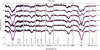 |
Fig. 2. Comparison of the best-fit model generated from the GA and SPAMMS for V382 Cyg. The best-fit solution from the GA is plotted in blue, the solution from SPAMMS is plotted in red, and the observed spectrum is plotted in black for several orbital phases, which are indicated at the right of the plot. The locations of relevant spectral lines are indicated by vertical dashed lines. |
The resulting best-fit parameters derived using the two methods agree more or less. The temperatures measured using SPAMMS appear to be systematically higher than those derived using the GA, but the effect appears small (∼1000 K). As demonstrated in Abdul-Masih et al. (2020), this is most likely an inclination effect: When compared with 1D fitting techniques, systems with high inclination will result in higher SPAMMS temperatures, while systems with low inclinations will result in lower SPAMMS temperatures. Equivalent temperatures are reached at about an inclination of 60°. This effect can be seen here, where V382 Cyg and SMC 108086 with inclinations of 85° and 82.5°, respectively, show higher temperatures measured using SPAMMS than with the GA, while VFTS 352, with an inclination of 55.6°, shows almost the exact same temperatures as measured using the two techniques.
The surface abundances also match well, but SPAMMS does not appear to reach the same level of precision as the GA for VFTS 352. This is most likely because the GA fit of VFTS 352 included the UV spectra, but the SPAMMS fit only included the optical spectra. Interestingly, however, the best-fit nitrogen surface abundance derived by SPAMMS for VFTS 352 appears to be more realistic than the best-fit solution from Abdul-Masih et al. (2019), which finds a nitrogen surface abundance well below the expected baseline value for the LMC. Similarly, in each of the three systems we studied, while the ranges of the surface abundances are in good agreement, the best-fit solutions within the ranges differ slightly between the two approaches. We note, however, that the surface abundances of carbon for V382 Cyg disagree: SPAMMS returns a higher carbon abundance than the GA by about half a dex.
While the error ranges for the helium surface abundance measured by SPAMMS and the GA overlap, SPAMMS measures very low helium surface abundances for V382 Cyg and VFTS 352. The values returned from the GA span a wider range and appear to be much more realistic than the values measured by SPAMMS, which are below the initial Big Bang helium abundance. One possible explanation for this arises from the fact that SPAMMS uses a fixed geometry and thus a fixed surface gravity structure across the surface. Because the surface gravity affects the ionization balance, the measured helium surface abundance might be raised and this issue fixed by including some of the binary parameters as free parameters, such as the component radii or the fillout factor. This would indicate that the confidence interval returned by SPAMMS for the helium surface abundances is most likely underestimated.
5.2. Evolutionary status
The first striking evolutionary question that arises from our spectroscopic analyses involves the fact that the spectral lines of the cooler component stars of V382 Cyg and SMC 108086 appear to be significantly broader than expected when tidal locking is assumed. For systems as close as these, the synchronization timescales are expected to be extremely short, so that we do not expect that they rotate asynchronously. On the other hand, recent studies have shown that ongoing mass transfer in unequal-mass ratio binaries can potentially lead to spin up for the mass gainer (Menon et al. 2020). The fact that two of the three systems in our sample require additional broadening to properly reproduce the observed spectra implies that these systems are still actively undergoing mass transfer, that the tidal effects behave differently in these systems, or that an additional unaccounted-for physical effect that mimics the effects of rotational broadening is present.
One potential explanation is macroturbulence, which we do not fit in this analysis. While the effects of macroturbulence and rotation on spectral lines can be degenerate with each other, the macroturbulence required to explain the observed difference is quite high. A comparison of the observed broadening with the tidally locked rotation rates implies that an additional broadening source of about 300 km s−1 or more is needed. Macroturbulence values for O- and B-type stars typically fall below ∼120 km s−1 (Simón-Díaz et al. 2017), but additional turbulent processes during the overcontact phase may justify these higher-than-expected values.
Because grids of evolutionary tracks suited for massive overcontact binaries are not fully developed yet, we compared our observations with single-star evolutionary tracks from Brott et al. (2011). While it is still debated which mixing mechanism is dominant in massive stars (see, e.g., Maeder 1987; Langer 2012; Bowman et al. 2019), we used the dense grid of rotation rates in the Brott et al. (2011) tracks as a proxy for internal mixing. Thus, higher rotation rates correspond to more internal mixing.
5.2.1. Surface abundances
Comparing the surface abundances measured using the GA and those measured using SPAMMS, we find that the two methods are reasonably consistent. Figures 5–7 show a comparison between the two methods for the carbon, nitrogen, and oxygen surface abundances. Evolutionary tracks corresponding to the component masses from Brott et al. (2011) are overplotted for various rotation rates. The confidence intervals for the GA and SPAMMS are indicated with shaded blue and red regions, respectively.
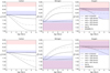 |
Fig. 5. Surface abundances for V382 Cyg of carbon (left), nitrogen (middle), and oxygen (right) for the primary (top) and secondary star (bottom) are plotted as a function of age. Single-star Galactic-metallicity evolutionary tracks from Brott et al. (2011; black lines) with initial masses of 25 M⊙ for the primary and 20 M⊙ for the secondary with various initial rotational velocities are overplotted. The shaded blue regions are the inferred range of surface abundances produced by the GA, and the shaded red regions are the surface abundance ranges produced by SPAMMS. The shaded region from the GA represent a 2σ confidence interval, and the shaded region from SPAMMS represents a 1σ confidence interval. |
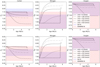 |
Fig. 6. Same as Fig. 5, but for VFTS 352. In this case, the Brott et al. (2011) tracks instead use an LMC metallicity and initial masses of 30 M⊙ for the primary and secondary. The GA results were taken from Abdul-Masih et al. (2019), who used a simultaneous UV and optical fit, and the SPAMMS fitting performed here only used the optical data. |
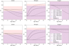 |
Fig. 7. Same as Fig. 5, but for SMC 108086. In this case, the Brott et al. (2011) tracks instead use an SMC metallicity and initial masses of 17 M⊙ for the primary and 15 M⊙ for the secondary. |
The upper and lower surface abundance limits for our SPAMMS input grid do not allow us to probe higher than 9.0 and lower than 6.0. All of our abundances are expected to be within this range, however. In some cases the confidence interval includes the upper or lower limit, so that in these cases, the confidence interval is underestimated. When we account for this, the ranges obtained from the GA and SPAMMS agree well. The largest differences can be seen in the carbon surface abundances, which are higher when fitting with SPAMMS for V382 Cyg. The opposite occurs for VFTS 352, but the line lists used for the GA and for SPAMMS are different in this case. Because the UV lines are affected by the winds, we did not fit them with the patch model, limiting our diagnostic lines to those in the optical portion of the spectrum. Additionally, because the optical data for VFTS 352 only extends to ∼4550 Å, we were unable to include several CNO lines that were included for the other two objects. The increased CNO abundance grid precision for the second round of SPAMMS fitting did not appear to change the best-fit values or the error bars in any of our runs, indicating that our initial grid precision of 0.5 dex is enough to accurately probe the parameter space when this method is used.
Compared with single-star evolutionary tracks, none of the systems show strong evidence of internal mixing when the surface abundance measurements are examined. V382 Cyg shows carbon, nitrogen, and oxygen all at baseline Galactic abundance without rotation (with the exception of the carbon abundance measured by SPAMMS, which is above the Galactic baseline instead of below, as expected from rotational mixing). The rotation rates for the primary and secondary derived from the GA and from SPAMMS indicate that the two components should fall somewhere between the ∼320 km s−1 and the ∼420 km s−1 lines. A comparison these rotation rates and the measured surface abundances with the Brott et al. (2011) evolution tracks indicates that the age of the system must be younger than one million years. As discussed in Abdul-Masih et al. (2019), VFTS 352 does not show strong signs of mixing in the CNO surface abundances either. Only the carbon abundance indicates possible depletion, but as discussed, the surface abundance derived from SPAMMS was based on a smaller line list only in the optical. The low metallicity and higher-than-expected rotation rates of the component stars in SMC 108086 make it difficult to constrain the surface abundances with the available data. The results from the GA indicate a slight depletion of carbon, but the confidence interval computed by SPAMMS extends up to the baseline. The confidence intervals for the nitrogen and oxygen surface abundances are also too wide to distinguish between the baseline and internal mixing cases for the GA and SPAMMS.
5.2.2. Location in the HRD
Figure 8 shows Hertzsprung–Russell diagrams (HRDs henceforth) corresponding to each object in our sample. This figure shows that all three overcontact systems studied here are highly overluminous and too hot for their current masses when compared to single-star evolutionary models. Furthermore, in all three cases, the primary and secondary components fall very close to each other on the HRD. In the case of VFTS 352, both components are of equal mass, therefore this is expected. However, for V382 Cyg and SMC 108086, the component masses are quite different, with mass ratios of 1.376 and 1.183, respectively (Martins et al. 2017; Hilditch et al. 2005). For V382 Cyg, the mass of the secondary is measured to be 19 M⊙ (Martins et al. 2017). Even with very efficient mixing, however, its location on the HRD cannot be reproduced with single-star evolutionary models, as was claimed by Martins et al. (2017). Instead, based on the temperature and luminosity, the less massive component falls closer to the evolutionary tracks corresponding to the more massive component than its own. The same can be seen in SMC 108086, where the secondary, with a measured mass of 14 M⊙ (Hilditch et al. 2005), falls along the 17 or 20 M⊙ tracks instead. These mass ratios come from the dynamical masses of these systems, which are widely considered more accurate and reliable than any other mass determination techniques (Serenelli et al. 2020). This indicates that the locations of the secondary components are indeed anomalous. The same conclusions can be reached when the locations of these objects on the log(g)−Teff plane are compared with expectations from evolutionary tracks, as shown in Fig. 9.
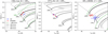 |
Fig. 8. Locations of each component of our sample in an HRD with Brott et al. (2011) evolutionary tracks corresponding to its metallicity. Objects and the component dynamic masses are labeled above each panel, and the Brott et al. (2011) evolutionary tracks at various rotation rates for various masses are plotted. Values and corresponding errors derived from the GA are plotted in blue and those from SPAMMS in red. The primary components are indicated with filled circles, and the secondaries are indicated with open squares. In the case of V382 Cyg and SMC 108086, rotating Geneva evolutionary tracks with initial masses of 40, 32, 25, and 20 for V382 Cyg (Ekström et al. 2012) and 20, 15, and 12 for SMC 108086 (Georgy et al. 2013) are plotted in green. |
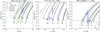 |
Fig. 9. Same as Fig. 8, but in the surface gravity versus effective temperature plane. In this case, only the values and corresponding errors derived from the GA are plotted because the surface gravity is not fitted with SPAMMS. The masses corresponding to each track are indicated below, each in their respective color in units of solar masses. |
As an independent verification of the object locations on the HRDs, we also calculated the luminosity of the components of each system based on its V-band magnitude, distance, and extinction. For V382 Cyg, we used the distance derived from Gaia early Data Release 3 (∼1.7 kpc Bailer-Jones et al. 2021), but because VFTS 352 and SMC 108086 are extragalactic systems, we instead used the distances derived from the Araucaria Project of 49.6 kpc (Pietrzyński et al. 2019) and 62.1 kpc (Graczyk et al. 2020) for the LMC and SMC, respectively. For all three components, we used the extinction from Maíz Apellániz & Barbá (2018), and we computed the bolometric corrections using the relation provided by Martins & Plez (2006) based on the effective temperature of the star. In this case, we used the temperatures derived from SPAMMS. For V382 Cyg, we find luminosities of log(Ldist/L⊙) ≈ 5.09 ± 0.05 and 5.10 ± 0.05 for the primary and secondary, respectively. For VFTS 352, we find luminosities of log(Ldist/L⊙) ≈ 5.24 ± 0.04 for the primary component and 5.16 ± 0.04 for secondary component. Finally, for SMC 108086, we calculated luminosities of log(Ldist/L⊙) ≈ 4.60 ± 0.03 and 4.66 ± 0.03 for the primary and secondary, respectively. All of these values agree very well with the values we calculated using the Stefan–Boltzmann law with the GA results and the modified Stefan–Boltzmann law using the SPAMMS results.
This leads to several interesting possible implications. Single-star evolutionary models show that the less massive component should not be able to reach the temperature observed at its surface. This means that the observed temperature of the secondary is either driven by the flux of the primary through irradiation or heat exchange in the shared envelope, or is driven by efficient mixing in the envelope through convection or large-scale circulations. If the flux from the primary were driving the temperature of the secondary through irradiation, then we might expect to see a region of lower temperature when the nonilluminated side of the secondary is facing toward us. This is not observed, but an indirect consequence of this mutual irradiation is a change in the net flux that leaves the irradiated regions of the star. If the fluxes leaving these regions are reduced and the overall luminosity remains constant, then the temperature of the entire star will increase slightly to compensate for this effect. This could partially explain the increased temperature observed in the secondary star.
Another potential way to obtain an overluminous secondary is efficient heat exchange through the common envelope. In the low-mass counterparts of massive overcontact binaries, namely W UMa systems, overluminous secondaries are observed often. In these systems, the overluminosity of the secondary is attributed to so-called sideways convection through the shared envelope (Lucy 1968a,b), with up to one-third of the energy generated by the primary being transported to the secondary (Mochnacki 1981). In the case of massive overcontact systems, the envelope is radiative instead of convective, so that a similar mechanism might be imagined involving heat transfer through radiation instead of convection.
Alternatively, this temperature increase could be explained by efficient internal mixing. In rapidly rotating single stars, the difference in temperature between the pole and equator is known to drive large-scale circulations in the envelope, known as Eddington–Sweet circulations (Eddington 1925; Sweet 1950). These occur because a rotating star cannot simultaneously be in hydrostatic and radiative thermal equilibrium (von Zeipel 1924). These Eddington–Sweet circulations operate along the temperature gradient and thus along meridional lines. Like rapidly rotating single stars, contact systems cannot simultaneously be in hydrostatic and radiative thermal equilibrium, and thus large-scale Eddington–Sweet-like circulations should operate. Unlike rotating single stars, however, contact systems are not azimuthally symmetric, meaning that these circulations will not necessarily operate along the meridional lines. This could allow heat exchange and material to be mixed through the bridge of the contact system and could explain the observed temperature profile. This effect can only be properly accounted for in 3D because it arises from the breaking of the polar and azimuthal symmetry. For a more in-depth discussion of this effect and its implications, see Hastings et al. (2020).
While mixing, heat transfer, and irradiation effects each could account for the increased temperatures and luminosities in the secondary, of the three mechanisms, only mixing is able to account for the increased luminosity of the system as a whole. Alternatively, this can be explained through nonconservative mass transfer as the stars initially come into contact. If some of the envelope of the donor star was ejected from the system, this would raise the overall mean molecular weight of the system, which would in turn increase the luminosity of both components. This would imply that the system started with a much higher total mass than is currently observed, and would suggest that some of this missing material may be observable in the surrounding environment. It is still unclear at the current time which mechanism or combination of mechanisms is responsible for these observed effects, however.
6. Conclusions
We have performed a full atmospheric analysis of three massive overcontact systems using two separate analysis methods. Using optical data sets, we performed fits using a standard one-dimensional approach and a more sophisticated 3D approach. We compared and contrasted the results of these two methods and find that while the 3D SPAMMS approach better reproduces the observed line profiles, the derived stellar parameters still agree fairly well with the 1D GA approach. We find an inclination-dependent variation in the derived temperatures, but we find that the surface abundances agree for the most part.
Our results indicate that the temperatures of unequal-mass overcontact systems do not behave as expected when compared with single-star evolutionary models: The temperatures of the components are similar and appear to be driven by the higher-mass component. Single-star evolutionary tracks that include rotation are not able to reproduce the location of the less massive object on the HRD. However, when the measured temperatures of the two components are plotted on the HRD, they are both consistent with the evolutionary tracks of the more massive component when high rotation rates (≳500 km s−1) are assumed. Additionally, we find that the two components of all three systems are highly overluminous, which is a potential indicator of internal mixing or nonconservative mass loss. Conversely, the surface abundance measurements do not show definitive signs of enhancements, giving further credence to the nonconservative mass-loss scenario.
When we compared our results with single-star evolutionary models and ignored binary effects such as mass exchange, the derived temperatures and luminosities appeared to indicate a different level of mixing than the derived surface abundances. If the temperatures and luminosities are considered alone, the internal mixing mechanisms appear to be efficient. However, if the surface abundances are considered alone, then there is no strong indication of mixing unless (i) the systems are very young or (ii) the component stars only began rapidly rotating after their chemical gradients were formed. It is unlikely that all stars in our sample are young, but it is unclear why these systems would begin rotating rapidly later in their lives. Despite this, it is still unclear how the systems can have such high temperatures but show little to no surface abundance deviations. Binary interaction effects most likely play a large role for these systems and could account for some if not all of the discrepancies discussed here. Alternatively, there may be additional unaccounted-for physical processes that are affected by the unique geometry of overcontact systems in a way we do not yet understand. More detailed evolutionary and stellar structure models of overcontact binaries are needed to compare our measurements. In addition, a more extensive line list and additional spectral data, especially in the UV, would allow us to better constrain the surface abundances and thus the evolutionary fate of these systems.
Acknowledgments
Based on observations obtained with the HERMES spectrograph, which is supported by the Fund for Scientific Research of Flanders (FWO), Belgium; the Research Council of KU Leuven, Belgium; the Fonds National de la Recherche Scientifique (F.R.S.-FNRS), Belgium; the Royal Observatory of Belgium; the Observatoire de Genève, Switzerland; and the Thüringer Landessternwarte Tautenburg, Germany. This work is based on data obtained at the European Southern Observatory under program IDs. 0103.D-0237, 182.D-0222, 090.D-0323, and 092.D-0136. We acknowledge support from the FWO-Odysseus program under project G0F8H6N. This project has received funding from the European Research Council under European Union’s Horizon 2020 research programme (grant agreement No. 772225). The computational resources and services used in this work were provided by the VSC (Flemish Supercomputer Center), funded by the Research Foundation – Flanders (FWO) and the Flemish Government. S.d.M.A.M. and S.J. were funded in part by the European Union’s Horizon 2020 research and innovation program from the European Research Council (ERC, Grant agreement No. 715063, PI de Mink), and by the Netherlands Organization for Scientific Research (NWO) as part of the Vidi research program BinWaves (639.042.728, PI de Mink). PM acknowledges support from the FWO junior postdoctoral fellowship No. 12ZY520N. L.M. thanks the European Space Agency (ESA) and the Belgian Federal Science Policy Office (BELSPO) for their support in the framework of the PRODEX Programme.
References
- Abdul-Masih, M., Sana, H., Sundqvist, J., et al. 2019, ApJ, 880, 115 [NASA ADS] [CrossRef] [Google Scholar]
- Abdul-Masih, M., Sana, H., Conroy, K. E., et al. 2020, A&A, 636, A59 [CrossRef] [EDP Sciences] [Google Scholar]
- Almeida, L. A., Sana, H., de Mink, S. E., et al. 2015, ApJ, 812, 102 [NASA ADS] [CrossRef] [Google Scholar]
- Almeida, L. A., Sana, H., Taylor, W., et al. 2017, A&A, 598, A84 [NASA ADS] [CrossRef] [EDP Sciences] [Google Scholar]
- Bailer-Jones, C. A. L., Rybizki, J., Fouesneau, M., Demleitner, M., & Andrae, R. 2021, AJ, 161, 147 [Google Scholar]
- Björklund, R., Sundqvist, J. O., Puls, J., & Najarro, F. 2021, A&A, 648, A36 [EDP Sciences] [Google Scholar]
- Bowman, D. M., Burssens, S., Pedersen, M. G., et al. 2019, Nat. Astron., 3, 760 [NASA ADS] [CrossRef] [Google Scholar]
- Bresolin, F., Crowther, P., & Puls, J. 2008, in Massive Stars as Cosmic Engines, IAU Symp., 250 [Google Scholar]
- Brott, I., de Mink, S. E., Cantiello, M., et al. 2011, A&A, 530, A115 [NASA ADS] [CrossRef] [EDP Sciences] [Google Scholar]
- Castor, J. I., Abbott, D. C., & Klein, R. I. 1975, ApJ, 195, 157 [NASA ADS] [CrossRef] [Google Scholar]
- Cester, B., Fedel, B., Giuricin, G., Mardirossian, F., & Mezzetti, M. 1978, A&AS, 33, 91 [NASA ADS] [Google Scholar]
- Charbonneau, P. 1995, ApJS, 101, 309 [Google Scholar]
- Conroy, K. E., Kochoska, A., Hey, D., et al. 2020, ApJS, 250, 34 [Google Scholar]
- Darwin, C. 1859, On the Origin of Species by Means of Natural Selection (London: Murray) [Google Scholar]
- de Mink, S. E., & Mandel, I. 2016, MNRAS, 460, 3545 [Google Scholar]
- de Mink, S. E., Pols, O. R., & Hilditch, R. W. 2007, A&A, 467, 1181 [NASA ADS] [CrossRef] [EDP Sciences] [Google Scholar]
- de Mink, S. E., Cantiello, M., Langer, N., et al. 2009, A&A, 497, 243 [NASA ADS] [CrossRef] [EDP Sciences] [Google Scholar]
- Deǧirmenci, Ö. L., Sezer, C., Demircan, O., et al. 1999, A&As, 134, 327 [NASA ADS] [CrossRef] [EDP Sciences] [Google Scholar]
- du Buisson, L., Marchant, P., Podsiadlowski, P., et al. 2020, MNRAS, 499, 5941 [Google Scholar]
- Eddington, A. S. 1925, The Observatory, 48, 73 [NASA ADS] [Google Scholar]
- Eggen, O. J., & Iben, I., Jr 1989, AJ, 97, 431 [Google Scholar]
- Ekström, S., Georgy, C., Eggenberger, P., et al. 2012, A&A, 537, A146 [NASA ADS] [CrossRef] [EDP Sciences] [Google Scholar]
- Freudling, W., Romaniello, M., Bramich, D. M., et al. 2013, A&A, 559, A96 [NASA ADS] [CrossRef] [EDP Sciences] [Google Scholar]
- Georgy, C., Ekström, S., Eggenberger, P., et al. 2013, A&A, 558, A103 [NASA ADS] [CrossRef] [EDP Sciences] [Google Scholar]
- Graczyk, D., Pietrzyński, G., Thompson, I. B., et al. 2020, ApJ, 904, 13 [Google Scholar]
- Hadrava, P. 1995, A&AS, 114, 393 [NASA ADS] [Google Scholar]
- Hadrava, P. 2009, ArXiv e-prints [arXiv:0909.0172] [Google Scholar]
- Hastings, B., Langer, N., & Koenigsberger, G. 2020, A&A, 641, A86 [EDP Sciences] [Google Scholar]
- Hilditch, R. W., Howarth, I. D., & Harries, T. J. 2005, MNRAS, 357, 304 [Google Scholar]
- Horvat, M., Conroy, K. E., Pablo, H., et al. 2018, ApJS, 237, 26 [Google Scholar]
- Howarth, I. D., Dufton, P. L., Dunstall, P. R., et al. 2015, A&A, 582, A73 [NASA ADS] [CrossRef] [EDP Sciences] [Google Scholar]
- Ilijic, S., Hensberge, H., Pavlovski, K., & Freyhammer, L. M. 2004, in Spectroscopically and Spatially Resolving the Components of the Close Binary Stars, eds. R. W. Hilditch, H. Hensberge, & K. Pavlovski, ASP Conf. Ser., 318, 111 [Google Scholar]
- Janssens, S., Shenar, T., Mahy, L., et al. 2021, A&A, 646, A33 [EDP Sciences] [Google Scholar]
- Jones, D., Conroy, K. E., Horvat, M., et al. 2020, ApJS, 247, 63 [Google Scholar]
- Justham, S., Podsiadlowski, P., & Vink, J. S. 2014, ApJ, 796, 121 [Google Scholar]
- Langer, N. 2012, ARA&A, 50, 107 [Google Scholar]
- Leung, K. C., & Schneider, D. P. 1978, ApJ, 222, 924 [Google Scholar]
- Lorenzo, J., Negueruela, I., Baker, A. K. F. V., et al. 2014, A&A, 572, A110 [NASA ADS] [CrossRef] [EDP Sciences] [Google Scholar]
- Lorenzo, J., Simón-Díaz, S., Negueruela, I., et al. 2017, A&A, 606, A54 [NASA ADS] [CrossRef] [EDP Sciences] [Google Scholar]
- Lucy, L. B. 1968a, ApJ, 153, 877 [Google Scholar]
- Lucy, L. B. 1968b, ApJ, 151, 1123 [Google Scholar]
- Maeder, A. 1987, A&A, 178, 159 [NASA ADS] [Google Scholar]
- Mahy, L., Sana, H., Abdul-Masih, M., et al. 2020a, A&A, 634, A118 [NASA ADS] [CrossRef] [EDP Sciences] [Google Scholar]
- Mahy, L., Almeida, L. A., Sana, H., et al. 2020b, A&A, 634, A119 [NASA ADS] [CrossRef] [EDP Sciences] [Google Scholar]
- Maíz Apellániz, J., & Barbá, R. H. 2018, A&A, 613, A9 [NASA ADS] [CrossRef] [EDP Sciences] [Google Scholar]
- Mandel, I., & de Mink, S. E. 2016, MNRAS, 458, 2634 [NASA ADS] [CrossRef] [Google Scholar]
- Marchant, P., Langer, N., Podsiadlowski, P., Tauris, T. M., & Moriya, T. J. 2016, A&A, 588, A50 [NASA ADS] [CrossRef] [EDP Sciences] [Google Scholar]
- Martins, F., & Plez, B. 2006, A&A, 457, 637 [NASA ADS] [CrossRef] [EDP Sciences] [Google Scholar]
- Martins, F., Mahy, L., & Hervé, A. 2017, A&A, 607, A82 [NASA ADS] [CrossRef] [EDP Sciences] [Google Scholar]
- Mateo, M., Harris, H. C., Nemec, J., & Olszewski, E. W. 1990, AJ, 100, 469 [Google Scholar]
- Menon, P. K., de Mink, S. E., Langer, N., et al. 2020, arXiv e-prints, [arXiv:2011.13459] [Google Scholar]
- Mochnacki, S. W. 1981, ApJ, 245, 650 [Google Scholar]
- Mochnacki, S. W., & Doughty, N. A. 1972, MNRAS, 156, 51 [Google Scholar]
- Mokiem, M. R., de Koter, A., Puls, J., et al. 2005, A&A, 441, 711 [NASA ADS] [CrossRef] [EDP Sciences] [Google Scholar]
- Mokiem, M. R., de Koter, A., Evans, C. J., et al. 2006, A&A, 456, 1131 [NASA ADS] [CrossRef] [EDP Sciences] [Google Scholar]
- Mokiem, M. R., de Koter, A., Evans, C. J., et al. 2007, A&A, 465, 1003 [NASA ADS] [CrossRef] [EDP Sciences] [Google Scholar]
- Pavlovski, K., & Hensberge, H. 2010, in Binaries - Key to Comprehension of the Universe, eds. A. Prša, & M. Zejda, ASP Conf. Ser., 435, 207 [Google Scholar]
- Pawlak, M., Soszyński, I., Udalski, A., et al. 2016, Acta Astron., 66, 421 [Google Scholar]
- Penny, L. R., Ouzts, C., & Gies, D. R. 2008, ApJ, 681, 554 [Google Scholar]
- Pietrzyński, G., Graczyk, D., Gallenne, A., et al. 2019, Nature, 567, 200 [Google Scholar]
- Pols, O. R. 1994, A&A, 290, 119 [Google Scholar]
- Popper, D. M. 1978, ApJ, 220, L11 [Google Scholar]
- Prša, A., Conroy, K. E., Horvat, M., et al. 2016, ApJS, 227, 29 [NASA ADS] [CrossRef] [Google Scholar]
- Puls, J., Urbaneja, M. A., Venero, R., et al. 2005, A&A, 435, 669 [NASA ADS] [CrossRef] [EDP Sciences] [Google Scholar]
- Puls, J., Vink, J. S., & Najarro, F. 2008, A&AR, 16, 209 [Google Scholar]
- Ramírez-Agudelo, O. H., Sana, H., de Koter, A., et al. 2017, A&A, 600, A81 [NASA ADS] [CrossRef] [EDP Sciences] [Google Scholar]
- Raskin, G., van Winckel, H., Hensberge, H., et al. 2011, A&A, 526, A69 [NASA ADS] [CrossRef] [EDP Sciences] [Google Scholar]
- Repolust, T., Puls, J., & Herrero, A. 2004, A&A, 415, 349 [NASA ADS] [CrossRef] [EDP Sciences] [Google Scholar]
- Riley, J., Mandel, I., Marchant, P., et al. 2021, MNRAS, 505, 663 [Google Scholar]
- Sana, H., & Evans, C. J. 2011, in Active OB Stars: Structure, Evolution, Mass Loss, and Critical Limits, eds. C. Neiner, G. Wade, G. Meynet, & G. Peters, 272, 474 [Google Scholar]
- Sana, H., de Mink, S. E., de Koter, A., et al. 2012, Science, 337, 444 [Google Scholar]
- Schneider, F. R. N., Ohlmann, S. T., Podsiadlowski, P., et al. 2019, Nature, 574, 211 [Google Scholar]
- Sekaran, S., Tkachenko, A., Abdul-Masih, M., et al. 2020, A&A, 643, A162 [EDP Sciences] [Google Scholar]
- Serenelli, A., Weiss, A., Aerts, C., et al. 2020, A&ARv, 29, 4 [Google Scholar]
- Shao, Y., & Li, X.-D. 2014, ApJ, 796, 37 [Google Scholar]
- Simon, K. P., & Sturm, E. 1994, A&A, 281, 286 [NASA ADS] [Google Scholar]
- Simón-Díaz, S., Godart, M., Castro, N., et al. 2017, A&A, 597, A22 [NASA ADS] [CrossRef] [EDP Sciences] [Google Scholar]
- Škoda, P., Hadrava, P., & Fuchs, J. 2012, in From Interacting Binaries to Exoplanets: Essential Modeling Tools, eds. M. T. Richards, & I. Hubeny, 282, 403 [Google Scholar]
- Smith, N., Andrews, J. E., Rest, A., et al. 2018, MNRAS, 480, 1466 [Google Scholar]
- Sundqvist, J. O., & Puls, J. 2018, A&A, 619, A59 [NASA ADS] [CrossRef] [EDP Sciences] [Google Scholar]
- Sweet, P. A. 1950, MNRAS, 110, 548 [Google Scholar]
- Szécsi, D., Langer, N., Yoon, S.-C., et al. 2015, A&A, 581, A15 [NASA ADS] [CrossRef] [EDP Sciences] [Google Scholar]
- Tkachenko, A. 2015, A&A, 581, A129 [NASA ADS] [CrossRef] [EDP Sciences] [Google Scholar]
- Tramper, F., Sana, H., de Koter, A., & Kaper, L. 2011, ApJ, 741, L8 [Google Scholar]
- Tramper, F., Sana, H., de Koter, A., Kaper, L., & Ramírez-Agudelo, O. H. 2014, A&A, 572, A36 [NASA ADS] [CrossRef] [EDP Sciences] [Google Scholar]
- Vernet, J., Dekker, H., D’Odorico, S., et al. 2011, A&A, 536, A105 [NASA ADS] [CrossRef] [EDP Sciences] [Google Scholar]
- Vink, J. S., de Koter, A., & Lamers, H. J. G. L. M. 2001, A&A, 369, 574 [NASA ADS] [CrossRef] [EDP Sciences] [Google Scholar]
- von Zeipel, H. 1924, MNRAS, 84, 665 [Google Scholar]
- Wellstein, S., Langer, N., & Braun, H. 2001, A&A, 369, 939 [NASA ADS] [CrossRef] [EDP Sciences] [Google Scholar]
- Woosley, S. E., & Heger, A. 2006, ApJ, 637, 914 [Google Scholar]
- Yoon, S. C., Langer, N., & Norman, C. 2006, A&A, 460, 199 [NASA ADS] [CrossRef] [EDP Sciences] [Google Scholar]
Appendix A: GA result plots
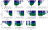 |
Fig. A.1. V382 Cyg Primary component: eleven-dimension chi-square merit surface projected along the individual parameter axis. All computed FASTWIND models are included. The confidence interval is indicated with shaded areas, while the model with the best chi-square is indicated by a vertical (black) line within the shaded areas. It is also given at the bottom of each panel. |
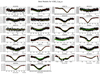 |
Fig. A.2. V382 Cyg Primary component: line profile fits corresponding to the best-fit solution in red and all models in the confidence interval that fulfill the cutoff plotted in green. The observed spectra and corresponding errors are plotted in black. The lines are labeled above each panel. |
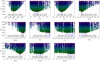 |
Fig. A.3. V382 Cyg Secondary component: same as Fig. A.1, but for the secondary component of V382 Cyg. |
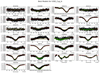 |
Fig. A.4. V382 Cyg Secondary component: Same as Fig. A.2, but for the secondary component of V382 Cyg. |
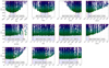 |
Fig. A.5. SMC 108086 Primary component: same as Fig. A.1, but for the primary component of SMC 108086. |
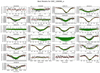 |
Fig. A.6. SMC 108086 Primary component: same as Fig. A.2, but for the primary component of SMC 108086. |
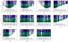 |
Fig. A.7. SMC 108086 Secondary component: same as Fig. A.1, but for the secondary component of SMC 108086. |
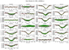 |
Fig. A.8. SMC 108086 Secondary component: same as Fig. A.2, but for the secondary component of SMC 108086. |
Appendix B: SPAMMS result plots
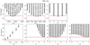 |
Fig. B.1. Seven-dimension chi-square merit surface projected along the individual parameter axis for V382 Cyg. All computed SPAMMS models are included. This run consists of a combination of three separate optimizations: the first for the temperature and asynchronisity parameter (top row), the second for the helium abundance (bottom row, leftmost panel) and third for the CNO abundances (bottom row, three rightmost panels). The dashed lines trace the chi-square-merit surface and the horizontal red line indicates the 1σ limit. |
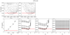 |
Fig. B.2. Same as Fig. B.1, but for VFTS 352. In this case, the asynchronisity parameters were not included in the optimization. |
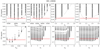 |
Fig. B.3. Same as Fig. B.1, but for SMC 108086. In this case, the asynchronisity parameters were included in the optimization for the primary and secondary. |
All Tables
Orbital solutions for V382 Cyg (Martins et al. 2017), VFTS 352 (Almeida et al. 2015), and SMC 108086 (Hilditch et al. 2005).
Results of the spherical GA analysis for the primary and secondary components of the systems in our sample.
Reference baseline surface abundances for helium, carbon, nitrogen, and oxygen for the Milky Way, LMC, and SMC.
All Figures
|
Fig. 1. PHOEBE II mesh model of V382 Cyg (left), VFTS 352 (center), and SMC 108086 (right). The mesh color represents the local effective temperature; lighter colors represent higher temperatures and darker colors represent lower temperatures. The systems have been inclined based on the system inclinations as given in Table 1. |
| In the text | |
|
Fig. 2. Comparison of the best-fit model generated from the GA and SPAMMS for V382 Cyg. The best-fit solution from the GA is plotted in blue, the solution from SPAMMS is plotted in red, and the observed spectrum is plotted in black for several orbital phases, which are indicated at the right of the plot. The locations of relevant spectral lines are indicated by vertical dashed lines. |
| In the text | |
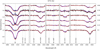 |
Fig. 3. Same as Fig. 2, but for VFTS 352. |
| In the text | |
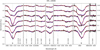 |
Fig. 4. Same as Fig. 2, but for SMC 108086. |
| In the text | |
|
Fig. 5. Surface abundances for V382 Cyg of carbon (left), nitrogen (middle), and oxygen (right) for the primary (top) and secondary star (bottom) are plotted as a function of age. Single-star Galactic-metallicity evolutionary tracks from Brott et al. (2011; black lines) with initial masses of 25 M⊙ for the primary and 20 M⊙ for the secondary with various initial rotational velocities are overplotted. The shaded blue regions are the inferred range of surface abundances produced by the GA, and the shaded red regions are the surface abundance ranges produced by SPAMMS. The shaded region from the GA represent a 2σ confidence interval, and the shaded region from SPAMMS represents a 1σ confidence interval. |
| In the text | |
|
Fig. 6. Same as Fig. 5, but for VFTS 352. In this case, the Brott et al. (2011) tracks instead use an LMC metallicity and initial masses of 30 M⊙ for the primary and secondary. The GA results were taken from Abdul-Masih et al. (2019), who used a simultaneous UV and optical fit, and the SPAMMS fitting performed here only used the optical data. |
| In the text | |
|
Fig. 7. Same as Fig. 5, but for SMC 108086. In this case, the Brott et al. (2011) tracks instead use an SMC metallicity and initial masses of 17 M⊙ for the primary and 15 M⊙ for the secondary. |
| In the text | |
|
Fig. 8. Locations of each component of our sample in an HRD with Brott et al. (2011) evolutionary tracks corresponding to its metallicity. Objects and the component dynamic masses are labeled above each panel, and the Brott et al. (2011) evolutionary tracks at various rotation rates for various masses are plotted. Values and corresponding errors derived from the GA are plotted in blue and those from SPAMMS in red. The primary components are indicated with filled circles, and the secondaries are indicated with open squares. In the case of V382 Cyg and SMC 108086, rotating Geneva evolutionary tracks with initial masses of 40, 32, 25, and 20 for V382 Cyg (Ekström et al. 2012) and 20, 15, and 12 for SMC 108086 (Georgy et al. 2013) are plotted in green. |
| In the text | |
|
Fig. 9. Same as Fig. 8, but in the surface gravity versus effective temperature plane. In this case, only the values and corresponding errors derived from the GA are plotted because the surface gravity is not fitted with SPAMMS. The masses corresponding to each track are indicated below, each in their respective color in units of solar masses. |
| In the text | |
|
Fig. A.1. V382 Cyg Primary component: eleven-dimension chi-square merit surface projected along the individual parameter axis. All computed FASTWIND models are included. The confidence interval is indicated with shaded areas, while the model with the best chi-square is indicated by a vertical (black) line within the shaded areas. It is also given at the bottom of each panel. |
| In the text | |
|
Fig. A.2. V382 Cyg Primary component: line profile fits corresponding to the best-fit solution in red and all models in the confidence interval that fulfill the cutoff plotted in green. The observed spectra and corresponding errors are plotted in black. The lines are labeled above each panel. |
| In the text | |
|
Fig. A.3. V382 Cyg Secondary component: same as Fig. A.1, but for the secondary component of V382 Cyg. |
| In the text | |
|
Fig. A.4. V382 Cyg Secondary component: Same as Fig. A.2, but for the secondary component of V382 Cyg. |
| In the text | |
|
Fig. A.5. SMC 108086 Primary component: same as Fig. A.1, but for the primary component of SMC 108086. |
| In the text | |
|
Fig. A.6. SMC 108086 Primary component: same as Fig. A.2, but for the primary component of SMC 108086. |
| In the text | |
|
Fig. A.7. SMC 108086 Secondary component: same as Fig. A.1, but for the secondary component of SMC 108086. |
| In the text | |
|
Fig. A.8. SMC 108086 Secondary component: same as Fig. A.2, but for the secondary component of SMC 108086. |
| In the text | |
|
Fig. B.1. Seven-dimension chi-square merit surface projected along the individual parameter axis for V382 Cyg. All computed SPAMMS models are included. This run consists of a combination of three separate optimizations: the first for the temperature and asynchronisity parameter (top row), the second for the helium abundance (bottom row, leftmost panel) and third for the CNO abundances (bottom row, three rightmost panels). The dashed lines trace the chi-square-merit surface and the horizontal red line indicates the 1σ limit. |
| In the text | |
|
Fig. B.2. Same as Fig. B.1, but for VFTS 352. In this case, the asynchronisity parameters were not included in the optimization. |
| In the text | |
|
Fig. B.3. Same as Fig. B.1, but for SMC 108086. In this case, the asynchronisity parameters were included in the optimization for the primary and secondary. |
| In the text | |
Current usage metrics show cumulative count of Article Views (full-text article views including HTML views, PDF and ePub downloads, according to the available data) and Abstracts Views on Vision4Press platform.
Data correspond to usage on the plateform after 2015. The current usage metrics is available 48-96 hours after online publication and is updated daily on week days.
Initial download of the metrics may take a while.