| Issue |
A&A
Volume 690, October 2024
|
|
|---|---|---|
| Article Number | A126 | |
| Number of page(s) | 18 | |
| Section | Stellar atmospheres | |
| DOI | https://doi.org/10.1051/0004-6361/202348478 | |
| Published online | 04 October 2024 | |
Empirical mass-loss rates and clumping properties of O-type stars in the Large Magellanic Cloud
1
Institute of Astronomy, KU Leuven,
Celestijnenlaan 200D,
3001
Leuven,
Belgium
2
Space Telescope Science Institute,
3700 San Martin Drive,
Baltimore,
MD
21218,
USA
3
Royal Observatory of Belgium,
Avenue Circulaire/Ringlaan 3,
1180
Brussels,
Belgium
4
European Southern Observatory,
Alonso de Cordova 3107, Vitacura,
Casilla
19001,
Santiago de Chile,
Chile
5
Instituto de Astrofísica de Canarias,
C. Vía Láctea, s/n,
38205
La Laguna,
Santa Cruz de Tenerife,
Spain
6
Universidad de La Laguna, Dpto. Astrofísica,
Av. Astrofísico Fran- cisco Sánchez,
38206
La Laguna,
Santa Cruz de Tenerife,
Spain
7
Astronomical Institute Anton Pannekoek, Amsterdam University,
Science Park 904,
1098 XH
Amsterdam,
The Netherlands
8
LMU München, Universitätssternwarte,
Scheinerstr. 1,
81679
München,
Germany
★ Corresponding author; This email address is being protected from spambots. You need JavaScript enabled to view it.
Received:
2
November
2023
Accepted:
8
July
2024
Abstract
Context. The nature of mass-loss in massive stars is one of the most important and difficult to constrain processes in the evolution of massive stars. The largest observational uncertainties are related to the influence of metallicity and wind structure with optically thick clumps.
Aims. We aim to constrain the wind parameters of sample of 18 O-type stars in the LMC, through analysis with stellar atmosphere and wind models including the effects of optically thick clumping. This will allow us to determine the most accurate spectroscopic mass-loss and wind structure properties of massive stars at sub-solar metallicity to date. This will allow us to gain insight into the impact of metallicity on massive stellar winds.
Methods. Combining high signal to noise (S/N) ratio observations in the ultraviolet and optical wavelength ranges gives us access to diagnostics of multiple different ongoing physical processes in the stellar wind. We produce synthetic spectra using the stellar atmosphere modelling code FASTWIND, and reproduce the observed spectra using a genetic algorithm based fitting technique to optimise the input parameters.
Results. We empirically constrain 15 physical parameters associated with the stellar and wind properties of O-type stars from the dwarf, giant and supergiant luminosity classes. These include temperature, surface gravity, surface abundances, rotation, macroturbulence and wind parameters.
Conclusions. We find, on average, mass-loss rates a factor of 4–5 lower than those from theoretical predictions commonly used in stellar-evolution calculations, but in good agreement with more recent theoretical predictions. In the ‘weak-wind’ regime we find massloss rates orders of magnitude below any theoretical predictions. We find a positive correlation of clumping factors with effective temperature with an average fcl = 14 ± 8 for the full sample. It is clear that there is a difference in the porosity of the wind in velocity space, and interclump density, above and below a temperature of roughly 38 kK. Above 38 kK an average 46 ± 24% of the wind velocity span is covered by clumps and the interclump density is 10–30% of the mean wind. Below an effective temperature of roughly 38 kK there must be additional light leakage for supergiants. For dwarf stars at low temperatures there is a statistical preference for very low clump velocity spans, however it is unclear if this can be physically motivated as there are no clearly observable wind signatures in UV diagnostics.
Key words: stars: atmospheres / stars: early-type / stars: fundamental parameters / stars: massive / stars: mass-loss / stars: winds, outflows
© The Authors 2024
 Open Access article, published by EDP Sciences, under the terms of the Creative Commons Attribution License (https://creativecommons.org/licenses/by/4.0), which permits unrestricted use, distribution, and reproduction in any medium, provided the original work is properly cited.
This article is published in open access under the Subscribe to Open model. This email address is being protected from spambots. You need JavaScript enabled to view it. to support open access publication.
1 Introduction
The mass-loss rates of hot OB type stars (Mini > 8 M⊙) are one of the paramount parameters in our understanding of massive stars, with a substantial influence on the course of the stellar evolutionary pathway, and yet they remain one of the most uncertain elements in stellar modelling (see reviews by Puls et al. 2008; Langer 2012; Smith 2014; and Vink 2022). The uncertainty is highlighted not only in stellar evolution but also in the statistical predictions of end-of-life products, including exotic and energetic objects such as stellar-mass black holes and gravitational wave events. Stellar mass loss is also a major consideration in the evolution of the interstellar medium as it contributes significant amounts of mass, energy, and momentum (Weaver et al. 1977). This mass loss is associated with strong radiatively driven winds, which are powered by momentum transfer through scattering between the ultraviolet (UV) radiation field and metal resonance line transitions in the outer atmosphere (Castor et al. 1975). This process is known to be very effective as Doppler-shifted material can be further accelerated by light of a higher wavelength than that of the rest wavelength of the transition (Sobolev 1960). If even small perturbations are present at the onset of the outflows, this so-called line deshadowing leads to highly unstable winds (MacGregor et al. 1979; Carlberg 1980; Owocki & Rybicki 1984; Eversberg et al. 1998; Lépine & Moffat 2008). This instability gives rise to strong shocks that result in a multi-component wind structure comprised of dense, slow-moving clumps of material in which line opacities can increase, and an interclump medium occupied by under-dense high-velocity material, which allows greater photon escape (Owocki et al. 1988; Feldmeier 1995; Dessart & Owocki 2003; Sundqvist et al. 2010; Sundqvist & Owocki 2013; Driessen et al. 2019). The uncertainty in mass loss was identified thanks to a discrepancy between empirically derived mass-loss rates from different physical diagnostics. In spectroscopic studies, synthetic spectra are produced from a radiative transfer solution of unified stellar atmosphere and wind models that take into account the effects of non-local thermo-dynamic equilibrium (NLTE; e.g. CMFGEN Hillier & Miller 1998, PoWR Gräfener et al. 2002, or FASTWIND Puls et al. 2005). Generally, spectroscopic analyses assumed the wind to be a smooth outflow. This resulted in the mass-loss rates derived using optical recombination line profiles (which depend on density as ρ2) to be much larger than those determined using UV resonance lines (which depend linearly on ρ). However, as the effects of wind structure were included, in a simplified form accounting for enhanced density in clumps, the discrepancy was reduced. Some issues still remained; mainly, that the absorption of light emitted by high-velocity metal ions such as phosphorus was over-predicted (Pauldrach et al. 1994; Hillier et al. 2003; Fullerton et al. 2006; Bouret et al. 2012). This appears to be solved by the consideration of the velocity span of clumps, which is limited at high velocity, resulting in reduced absorption of blue-shifted light from these metal ion transitions (e.g. Oskinova et al. 2007; Sundqvist et al. 2010; Sundqvist et al. 2011; Šurlan et al. 2013; Hawcroft et al. 2021).
As empirical mass-loss rates generally began to converge with the inclusion of clumping corrections, there still remained a discrepancy when making comparisons with theoretical predictions. The magnitude of this varies in different physical regimes, but generally a factor of three was found for O-type stars (see e.g. Bouret et al. 2012; Hawcroft et al. 2021; Brands et al. 2022). This could not be attributed to wind clumping as clumping is thought to have little impact on theoretical predictions of mass loss (Muijres et al. 2011). The problem may come from physical assumptions in such model predictions as significantly different rates are predicted using different numerical techniques (Vink et al. 2001; Krtička & Kubát 2018; Björklund et al. 2021; Vink & Sander 2021; Björklund et al. 2023).
In the realm of typical O-stars (5.2 < log(L/L⊙) < 6.2), thanks to this inclusion of wind structure in spectroscopic models and new hydrodynamically consistent theoretical predictions, the mass-loss rates in theory and observations appear to be converging. Hawcroft et al. (2021) find mass-loss rates that are between a factor of two and three lower than the rates predicted by Vink et al. (2001) but that agree well with the predictions of Björklund et al. (2021) for a sample of Galactic O-supergiants. Brands et al. (2022) cover a larger range of O stars in the Large Magellanic Cloud (LMC), with a large representation of main-sequence O dwarfs. These authors find good agreement with Krtička & Kubát (2018) and Björklund et al. (2021) up to high luminosities (log(L/L⊙) > 6.2) at which there is better agreement with the predictions of Vink & Sander (2021), although the predictions must be extrapolated to these luminosities as the model grids in these works extend only up until log(L/L⊙) = 6.0. Higher-luminosity predictions are available from Vink (2018) but there are concerns regarding the validity of a steady-state approach in this regime (Jiang et al. 2018; Schultz et al. 2020). Uncertainty persists at high luminosity as stars approach the Eddington limit (Gräfener & Hamann 2008; Vink et al. 2011), although perhaps the largest remaining discrepancy is at low luminosities of log(L/L⊙) < 5.2. Mass-loss rates of late O dwarfs and giants are found to be orders of magnitudes lower than predicted (Bouret et al. 2003; Martins et al. 2004; Martins et al. 2005; Marcolino et al. 2009; de Almeida et al. 2019; Rubio-Díez et al. 2022; Brands et al. 2022).
Another major effect in our understanding of stellar winds is the metallicity dependence. As the chemical composition of the star changes, specifically as the abundance of key wind-driving metals varies, so should the strength of the wind. The aforementioned theoretical rates all predict a metallicity mass-loss relation, of the order of ~Z0.67 to ~Z0.95 (Vink et al. 2001; Krtička & Kubát 2018 and Björklund et al. 2021). This has been difficult to test empirically due to lack of simultaneous UV and optical coverage at low metallicity. Mokiem et al. (2007) used optical diagnostics to estimate the empirical  dependence, finding
  . Marcolino et al. (2022) also provide an empirical relation of
  for bright stars (log(L/L⊙) > 5.4), with a weaker dependence at lower luminosity. It is unclear whether the strength of the line-deshadowing instability (LDI), and therefore the wind structure, is likely to change with metal-licity or with other stellar parameters. While Brands et al. (2022) investigated wind properties in the LMC, it is difficult to draw conclusions as their sample follows a close positive relation between luminosity and temperature, meaning it is difficult to disentangle which parameter is leading the relation with wind properties. The only other attempts to constrain wind structure are studies of variability in emission-line profiles, through which it is possible to see the direct influence of clumps moving through the wind and shaping the profile over time. Using this method, Lépine & Moffat (2008) found no evidence of a change in clumping properties between Galactic O supergiants and Wolf-Rayet (WR) stars. Marchenko et al. (2007) studied three WR stars from the Small Magellanic Cloud (SMC) and again were unable to find evidence for changing clumping properties. Driessen et al. (2022) investigated the metallicity dependence of clumping properties theoretically using 2D LDI simulations of O-stars at fixed luminosity, and conclude that such a relation exists, although it is fairly weak: ƒcl ∝ Z0.15. These authors also note that this provides a moderate correction to the aforementioned empirical metallicity mass loss relation of Mokiem et al. (2007), which uses Hα diagnostics, resulting in
  . Finally, Driessen et al. (2022) find generally lower clumping factors relative to 1D simulations, as the added spatial dimension allows for some smoothing of the over-densities. It is thus likely that the clumping factors will decrease even further in 3D LDI simulations.
Another physical effect of low metallicity is faster rotation, due to the reduced mass loss at low metallicity resulting in less removal of angular momentum. This is thought to have implications for stellar evolution and internal mixing and has been studied rather more than the mass loss (e.g. Yoon et al. 2008; Hunter et al. 2009; Brott et al. 2011b; Rivero González et al. 2012a; Rivero González et al. 2012b; Bouret et al. 2013; Georgy et al. 2013; Ramírez-Agudelo et al. 2013; Ramírez-Agudelo et al. 2015; Grin et al. 2017; Keszthelyi et al. 2017; Groh et al. 2019; Bouret et al. 2021; Murphy et al. 2021; Eggenberger et al. 2021).
In this study, we focus on a sample of O stars, covering the luminosity range 5.2 < log(L/L⊙) < 6.0, in the LMC; in other words, at half the solar metallicity. For this, we have obtained UV spectroscopic observations of 18 O stars in the LMC (GO: 15629, PI: Mahy) and utilised archival optical coverage. This allows us to investigate stellar and wind parameters. For this analysis, we simultaneously determined a number of stellar properties, with a focus on investigating the mass-loss rates, clumping factors, and wind structure parameters with high accuracy across the upper part of the Hertzsprung-Russell diagram (HRD).
The paper progresses with a description of the sample and observations in Sect. 2. This is followed by a description of our modelling technique in Sect. 3. We present stellar and wind parameters in Sect. 4. In Sect. 5, we discuss our findings, with a focus on wind parameters. The paper concludes in Sect. 6.
Overview of the capability of the instruments used to obtain spectra for this sample.
2 Sample and observations
The sample of 18 LMC stars analysed in this work is distributed throughout the O-star spectral sub-types from early to late including: one supergiant, three bright giants, four giants, and ten dwarfs or sub-giants. The targets were selected from the VFTS catalogue (VLT-FLAMES Tarantula Survey, Evans et al. 2011). We also utilised the optical spectra obtained as part of VFTS in our fitting. The VFTS spectra were obtained using the Medusa mode of the ESO FLAMES instrument on the Very Large Telescope (VLT) combined with the GIRAFFE spectrograph. The LR02, LR03, and HR15N setups were used, delivering spectroscopy of key stellar and wind diagnostic spectral lines from 4000 to 4500 Å at a resolving power of ~7000, from 4500 to 5000 Å at a resolving power of ~8500 and at a resolving power of ~ 16 000 in the range from 6400 to 6800 Å. The VFTS observations are further detailed in Evans et al. (2011).
In order to capture essential wind diagnostics at UV wavelengths, a series of follow-up observations were carried out with the Hubble Space Telescope (HST). The majority of the observations were taken using the Cosmic Origins Spectrograph (COS), with six stars observed using the Space Telescope Imaging Spectrograph (STIS) due to the presence of bright stars surrounding the target. Table 1 shows the instruments used to obtain the observations for this work and their spectroscopic capabilities. Compared to Brands et al. (2022), the UV spectra we have obtained are of a higher resolution by roughly a factor of three, increasing the signal-to-noise (S/N) for each equivalent resolution element. This means we have higher S/N for low-luminosity (log(L/L⊙) < 5.2) stars, which allows us to constrain wind parameters for these types of stars for the first time. We have a smaller sample than Brands et al. (2022) (~20 compared to ~50), but a more even ratio of giants and bright giants to dwarfs, while the sample of Brands et al. (2022) primarily comprises dwarf stars. We also note that the complementary optical spectra are quite different between our work and Brands et al. (2022). These authors use optical spectra from HST-STIS as the focus is on the central core of the R136 cluster, which was excluded from the VFTS observing campaign due to crowding and can only be resolved with HST. As a result, the optical spectra used in Brands et al. (2022) are of lower resolving power and on average have S/N ~ 20, which is a factor of ten lower than those available in this study from VFTS (see Brands et al. (2022) for further details on the data used in their study). Typically, an S/N ~ 100–200 is required to constrain individual stellar parameters from optical spectra of O stars, with higher S/N required for fast rotators (v sin i > 200 km s−1, Grin et al. 2017).
The sample contains four stars (VFTS143, VFTS184, VFTS422, and VFTS608) with significant radial velocity variations and amplitudes large enough to fulfil the binarity criteria of Sana et al. (2013), although the nature of this variability is unconstrained. We therefore cannot make any systematic analysis of the influence of tentative binarity on global wind physics with this dataset but comment on whether this radial velocity variability has any impact on the fits for the relevant star in Appendix B. We also take care to select the stars such that the intrinsic spectral variability is small. All targets are far from the luminous blue variable (LBV) regime, and therefore the non-contemporaneity of the UV and optical observations will not affect the results and conclusions of the current study.
3 Methods
In order to determine stellar and wind parameters, we compared the observed spectra with synthetic spectra, produced using the code FASTWIND (v10.3, Santolaya-Rey et al. 1997; Puls et al. 2005; Rivero González et al. 2011; Carneiro et al. 2016; Sundqvist & Puls 2018), with the parameters of interest given as inputs. FASTWIND is a stellar atmosphere and wind modelling software that calculates model atmospheres, including the effects of line-blocking or blanketing for background ions, while giving a full co-moving frame transport treatment to explicit elements. Differentiating between these two groups of elements allows the code to treat relevant spectral diagnostics with high precision, while maintaining a performance speed that makes computing thousands of models per object entirely feasible. In this study, line transitions from H, He, C, N, O, P, and Si were treated as explicit elements. FASTWIND is uniquely suited for this analysis as it has the functionality to include clumps of arbitrary optical thickness and account for the effect of a highly structured wind on NLTE occupation numbers and the subsequent projection onto synthetic spectra by computing an effective opacity for the two-component outflow (consisting of dense clumps and an under-dense interclump medium). For further details on the clumping parameterisation in FASTWIND, we refer to Sundqvist & Puls (2018); Hawcroft et al. (2021); and Brands et al. (2022).
The speed of the atmosphere modelling code is a high priority in our analysis as we employed a computationally expensive fitting algorithm to simultaneously optimise all the stellar parameters. Our fitting technique was to use a genetic algorithm (GA), which is based on the principles of genetic evolution and adapted from the Pikaia code (Charbonneau 1995; Mokiem et al. 2005). Such a technique has been used successfully to determine stellar and wind parameters for various samples of massive stars (Mokiem et al. 2006; Mokiem et al. 2007; Tramper et al. 2011; Tramper et al. 2014; Ramírez-Agudelo et al. 2017; Abdul-Masih et al. 2019; Abdul-Masih et al. 2021; Hawcroft et al. 2021; Johnston et al. 2021; Fabry et al. 2021; Brands et al. 2022; Shenar et al. 2022). The version used in this study is the same as the one presented in Hawcroft et al. (2021).
The GA works by computing a large initial population of FASTWIND models spanning the full range of the parameter space1, and assessing the quality of their reproduction of the spectra using an χ2-based fitness metric in which all line profiles are weighted equally (see Eq. (7) in Hawcroft et al. 2021). These models are then selected in pairs and their parameters combined to create another generation of models, with selection preference given to models with higher fitness. This process is iterated until the fit to the data is no longer being improved significantly with each new generation. Various random mutations are applied to the model parameters at each generation to enhance the parameter space exploration.
Such a fitting technique is a marked improvement on the established ‘by-eye’ fitting method as there is now a consistent statistical evaluation criterion that we can use to assess fit quality. The process is also automated, allowing for a more thorough exploration of the parameter space. We note that equally high-quality fits can be found using the by-eye approach; Markova et al. (2020) found a good agreement between GA and by-eye fitting approaches. In both cases, appropriate spectral regions must be manually selected and prepared carefully (normalisation, contamination). In an additional pre-processing step, we removed clear instances of interstellar contamination so that these contributions were not reproduced by the automated fitting routine. This is most common in the case of nebular emission in the cores of optical hydrogen recombination lines. The final spectra used for the fits are shown throughout Appendix C and regions that have been removed are clearly visible.
We optimised a number of parameters using the GA and left others fixed following certain assumptions. Thirteen of these parameters are inputs to the FASTWIND code, including effective temperature and surface gravity. Four abundance parameters were used to determine the surface abundances of helium, nitrogen, carbon, and oxygen. The remaining FAST-WIND inputs are wind parameters, including the mass-loss rate,  , wind acceleration, β, terminal wind speed, v∞, and four clumping parameters. The clumping parameters are: the clumping factor, ƒcl, velocity filling factor, ƒvel, interclump density, ƒic and the clumping onset velocity, vcl (which can also be expressed as the clumping onset radius, Rcl, and which is defined further in Sect. 3.1 of Hawcroft et al. 2021). The final two free parameters are rotational and macroturbulent broadening, which were applied to the synthetic spectra produced by FASTWIND in post-processing before the fitness to observations was assessed. All models were computed with an LMC metallicity of Z = 0.5 Z⊙, meaning that all fixed abundances were scaled to half of solar, where Z⊙ was defined as in Asplund et al. (2009). Using a distance to the LMC of 50 kpc (Gibson 2000; Pietrzyński et al. 2019), Ks-band photometry (Kato et al. 2007; Evans et al. 2011), and an average K-band extinction (Ramírez-Agudelo et al. 2017), we estimated an absolute K-band magnitude, which worked as a calibration for the stellar radius in combination with an input effective temperature.
We adopted a microturbulent velocity of 10 km s−1 in the NLTE computation of FASTWIND, and during the formal integral we allowed the microturbulence to increase linearly with the wind speed as 0.1v, which results in an overall prescription of fixed microturbulence at the photosphere, which increases to a maximum in the outer wind at 0.1v∞. This approach was also taken in Abdul-Masih et al. (2021) and Hawcroft et al. (2021). Similarly, the clumping parameters begin increasing at the input onset velocity and increase linearly until they reach their maximum at twice the onset velocity. The maximum values of the clumping parameters are therefore the free parameters, and these best-fit maximum clumping parameters are listed in Tables 2 and A.1.
We do not include the effects of X-rays in our models. Therefore, we did not attempt to fit wind line profiles, which are sensitive to the X-ray luminosity; these include UV metal lines such as N V λλ 1239–1243.
We focused on a number of key line diagnostics, around which we optimised the fit. In the UV, we generally included He II λ1640, C IV λ1169, CIII λ1176, C IV λλ1548– 1551, C III λ1620, N IV λ1718, O IV λλ1340–1344, O V λ1371, Si IV λλ1394, 1403, and P V λλ1118–1128. In the optical, we have the Balmer series from Hα to Hδ, He I λ4009, He I+II λλ4025–4026, He I λ4471, He I λ4922, He II λ4200, He II λ4541, C III λλ4068–70, N III λλ4510–4514–4518, N III λλ-4634–4640–4642, and N IV λ4058. We note that some lines may be excluded or others included depending on spectral type. The full line list for each object can be seen in Appendix C.
Best-fit wind parameters from GA fitting including optically thick clumping.
 |
Fig. 1 Kiel diagram showing best-fit effective temperatures and surface gravities for the sample. The shapes represent the best-fit parameters from the GA. The blue squares are the supergiants, the orange triangles the giants and the green circles the dwarf stars. The crosses are literature measurements of the same parameters from Ramírez-Agudelo et al. (2017) (RA17) for (super)giants or Sabín-Sanjulián et al. (2017) (SS17) for dwarfs. Lines are drawn between points to guide the eye between measurements made for the same star from this work and literature studies. These are overplotted against evolutionary tracks from Brott et al. (2011a) at an LMC metallicity of Z = 0.5 Z⊙ and moderate rotation of v sin i ~ 150–200 km s−1. Each evolutionary track is annotated with the input initial stellar mass. |
4 Results
We obtained synthetic spectral best-fit solutions to high-resolution UV and optical spectra for 18 O-type stars. For each of these fits, we have optimised 15 input parameters describing the stellar and wind properties using the GA-based fitting technique described in Sect. 3. The final best-fit parameters are listed in Tables 2 and A.1. Individual fits and discussions thereof are included in Appendix B.
Uncertainties were obtained by considering all models within a 95% confidence interval of the best-fit model to be statistically equivalent solutions, as in previous GA studies (see e.g. Abdul-Masih et al. 2019; Hawcroft et al. 2021). As for the stellar radius (Reff, defined at a Rosseland optical depth of τ = 2/3), we followed the method of Repolust et al. (2004), Mokiem et al. (2005) and find the uncertainty to be dominated by the uncertainty in the K-band magnitude, which results in ∆R = 1.3 R⊙ generally corresponding to 10–20%, similar to the 15% found by Repolust et al. (2004) who used V-band magnitudes.
A number of stars analysed here have been investigated in previous spectroscopic studies. We are therefore able to compare our best-fit parameters to literature values for some fundamental stellar parameters, keeping in mind that there may be systematic discrepancies as these previous studies have been made using only optical spectra, without consideration of optically thick clumps and often with differing optimisation techniques. The four supergiants (or bright giants) were previously analysed by Ramírez-Agudelo et al. (2017) using a GA approach on only optical spectra. Two giants were also included in Ramírez-Agudelo et al. (2017), and the other two were studied by Bestenlehner et al. (2014) using a grid-based approach with CMFGEN models. Eight of the dwarfs are included in Sabín-Sanjulián et al. (2017), which uses a grid based approach to fit FASTWIND models to optical spectra. The two remaining dwarfs (VFTS143 and VFTS184) have not been included in any previous atmospheric analysis studies. A more thorough comparison with the literature is presented on a star-by-star basis in Appendix B; for this section, we briefly make a comparison with the fundamental spectral parameters, effective temperature, and surface gravity. We focus on the effective temperature and surface gravity here as significant discrepancies in these parameters between studies, without sufficient explanation, would require further investigation.
For most of the dwarf stars, we find effective temperatures that are in agreement with the spectral-type calibrations of Walborn et al. (2014) within 1 kK. The supergiants and giants that have literature properties are in generally good agreement with our findings, with differences in best-fit temperature and gravity on an individual basis that do not appear to be systematic, likely due to our inclusion of the UV diagnostics. This also seems to be the case for early dwarfs; however, there may be a systematic difference between our method and the grid-based approach of Sabín-Sanjulián et al. (2017) for late dwarfs. We find generally lower temperatures and surface gravities. These differences are shown in Fig. 1.
We include the surface abundances of carbon, nitrogen, and oxygen as free parameters in our fit optimisation, which provides important diagnostic information on CNO wind lines. We define, for example, є(C) as the ratio of the carbon to hydrogen abundance by number through є(C) = log(nC/nH)+12, where the baseline LMC CNO abundances are є(C)=7.75, є(N)=6.9, and є(O)=8.35 (Kurt & Dufour 1998; Brott et al. 2011a; Köhler et al. 2015). These abundances are primarily used to estimate the evolutionary status of massive stars as their ratios are expected to change as a result of the CNO cycle. We generally observe the expected enrichment with evolutionary stage (in that the ratios of N/C and N/O are larger for supergiants) but the only stars for which we can constrain these ratios relative to the values predicted for CNO processing, or even initial composition, are the supergiants and bright giants. For the rest of the sample, the uncertainties are too large to comment on the CNO processing. For a comprehensive study on the evolutionary status and surface abundances, a wider range of diagnostic line profiles for the relevant elements are required, and/or the contribution of these metal lines to the goodness of fit would need to be boosted relative to the strong wind line profiles. For our purposes, including the abundances allows us to assess the degeneracies between abundances and wind parameters, mainly to determine whether the abundances are affecting wind parameters, but this does not appear to be the case due to the aforementioned limited number of photospheric lines and their relative strengths.
For the mass-loss rates of stars with a higher luminosity (5.2 < log(L/L⊙) < 6.2), we find an average reduction of six times compared to theoretical predictions from Vink et al. (2001). The mass-loss rates we determine here are within 20% of the predictions from Björklund et al. (2021) on average. For low-luminosity stars (log(L/L⊙ < 5.2), we find very low mass-loss rates consistent with the ‘weak-wind’ problem (Martins et al. 2005; Marcolino et al. 2009; Najarro et al. 2011; de Almeida et al. 2019). However, this does not appear to be a universal issue, as we find two dwarfs at the edge of the canonical weak-wind regime with fairly typical mass-loss rates (VFTS184 and VFTS223).
5 Discussion
5.1 Mass-loss rates
Mass-loss rates determined with consistent fitting of UV and optical wind spectral features are thought to be closer to the true values, relative to mass-loss rates determined only using optical features. The mass-loss rate and clumping parameters are highly degenerate for diagnostics that are sensitive to the square of the density and so optical recombination lines (depending on ρ2) can only be used to constrain a combined  factor. Simultaneous UV fitting breaks this degeneracy as UV resonance wind lines depend only linearly on density. Therefore, with coverage of both processes we can accurately constrain the mass-loss rate and clumping factor. However, there are still problems in determining the mass-loss rates when assuming that the wind clumps are optically thin. This is highlighted, for example, by difficulties in fitting the absorption components of P V line profiles: generally, the phosphorus abundance has to be reduced to non-physical values or the mass-loss rates reduced to such a degree that there are issues in reproducing other UV lines (Pauldrach et al. 2001; Crowther et al. 2002; Hillier et al. 2003; Bouret et al. 2005, 2012). Recent progress has shown that an alternate solution is viable. It is possible to reproduce the P V profiles if a more detailed wind structure is considered, specifically the limited velocity span of the clumps, which allows for additional light leakage that can reduce the strength of absorption in high-velocity blue-shifted components of P-Cygni UV lines (Oskinova et al. 2007; Sundqvist et al. 2010, 2011; Šurlan et al. 2013). In addition, it has been shown that simultaneous fits to far-ultraviolet (FUV), UV, and optical wind features can be obtained when using a wind clumping prescription that allows clumps to become optically thick and considers clump velocity coverage and the density of the interclump medium (see Hawcroft et al. 2021 and Brands et al. 2022). The mass-loss rates presented here were determined with models including these effects, and the same method (GA fitting of UV and optical spectra) outlined in these previous studies.
We compare mass-loss rates found with the GA to the mass-loss rates predicted from theoretical recipes using the relevant GA best-fit parameters as inputs; this is shown in Fig. 2. For the portion of the sample with typical O star winds (log(L/L⊙) > 5.2), we find that the observationally derived rates are on average four times lower than those predicted using the Vink et al. (2001) rates. This is after accounting for the different metallicities used to compute the theoretical predictions, with Vink et al. (2001) using a solar metallicity of Z⊙ = 0.019 from Anders & Grevesse (1989), while Krtička & Kubát (2018) and Björklund et al. (2021) use Z⊙ = 0.013 from Asplund et al. (2009). However, this ~40% adjustment for input metallicity may be an over-correction, as Sundqvist et al. (2019) find only an ~20% difference in mass-loss rates computed with the two different input metallicities in their wind models. Therefore, the empirical mass-loss rates we find could be up to five times lower than the predictions from Vink et al. (2001). This factor of four is a slightly larger discrepancy than that found in previous studies. A reduction of a factor of three was found by Crowther et al. (2002) for LMC O-supergiants, a factor of three by Bouret et al. (2005) who studied an O dwarf and supergiant in the Galaxy, a factor of three by Bouret et al. (2003) for SMC O-dwarfs, a factor of three by Evans et al. (2004) for late O and early B-type supergiants in the LMC and SMC, a factor of two to three by Bouret et al. (2012) and Hawcroft et al. (2021) for Galactic O-supergiants, a factor of two by Brands et al. (2022) for O stars in the LMC, and a factor of three by Šurlan et al. (2013). Cohen et al. (2014) find a factor of three from X-ray diagnostics. Our results are also slightly lower than the factor-of-five reduction found by Massa et al. (2003) for LMC O-stars, which was a study using only UV spectra from the Far Ultraviolet Spectroscopic Explorer (FUSE). We find a mix of over- and under-predictions of mass-loss rates from Krtička & Kubát (2018) and Björklund et al. (2021), although the agreement is generally good. We assessed the ability of the predictions to reproduce the empirical results ( ,
,  ), finding the best agreement with the predictions from Krtička & Kubát (2018). This is similar to the results of Brands et al. (2022), who find a similar trend in goodness of fit between the predictions. We also compare the modified wind-momentum rate (Fig. 3) and find similar results.
Below a luminosity of log(L/L⊙) = 5.2, we notice a significant downward trend in derived mass-loss rates, entering the canonical weak-wind regime. Thanks to a combination of the flexibility of our fitting technique and sufficient computational resources, we were able to explore the lowest limit of the mass-loss rate within the capabilities of FASTWIND. The mass-loss rates we find for the weak-wind stars are between 10−9 and 10−11 M⊙ yr−1. This is much lower than those found for similar stars in the LMC in Brands et al. (2022), although this is likely only due to a lower range of mass-loss rates being considered, as these authors find uncertainties on the mass-loss rates for similar stars that extend to the lower limit of their parameter space. The rates we find are therefore also lower than equivalent Galactic stars, with dwarfs presented in Martins et al. (2005) and Marcolino et al. (2009), and giants analysed in Mahy et al. (2015) and de Almeida et al. (2019). Again, they are lower than the mass-loss rates of 10−9 and 10−8 M⊙ yr−1 found in late-type SMC dwarfs by Bouret et al. (2003) and Martins et al. (2004). The comparison between the mass-loss rates determined here and previous studies is generally more complex, as these studies do not account for optically thick clumps or wind porosity in velocity space (except Brands et al. 2022), although in the case of weak-wind stars we were unable to constrain these additional clumping parameters and so perhaps a more straightforward comparison can be made. The mass-loss rates we find in this regime are on average 270,140, and 30 times lower than theoretical predictions from Vink et al. (2001), Krtička & Kubát (2018), and Björklund et al. (2021), respectively. For two dwarf stars with 5-0 < log(L/L⊙) < 5.2, though, we find mass-loss rates that are not too far from the theoretical predictions, perhaps suggesting a gradual onset of the weak-wind problem. If we move these stars out of the weak-wind sample for the purpose of measuring average scalings, we have a reduction of 4.8 relative to Vink et al. (2001) for the typical O star, and a reduction of nearly 400 times in the weak-wind regime. There is little change to the average agreement with Björklund et al. (2021) and Krtička & Kubát (2018) for normal O stars ( and
and  ) but the discrepancy for weak-wind stars rises to a factor of 50 compared to Björklund et al. (2021) and a factor of 200 compared to Krtička & Kubát (2018). We note that there is a more significant change in the empirical trend for the modified wind-momentum rate when these two stars are included. Due to the lack of a wind-momentum recipe from the Krtička & Kubát (2018) models we cannot make comparisons for all predictions and so cannot quantify the best agreement with our empirical results, but qualitatively there is very good agreement with Björklund et al. (2021).
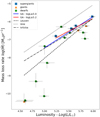 |
Fig. 2 Mass-loss rates from GA best fits. The supergiants are the blue squares, the giants are the orange triangles, and the dwarfs are the green circles. A linear fit to the GA best-fit mass-loss rates for stars with log(L/L⊙) ≥ 5.0 is shown by the solid line. Theoretical predictions tailored to our best-fit stellar parameters from Vink (Vink et al. 2001), Krtička (Krtička & Kubát 2018), and Leuven (Björklund et al. 2021) are shown in dotted, dash-dotted, and dashed lines, respectively. |
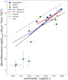 |
Fig. 3 Modified wind-momentum rate computed using GA best fit values compared to the predictions made by Leuven (Björklund et al. 2021), Krtička (Krtička & Kubát 2018), and Vink (Vink et al. 2001) for each star in our sample. Supergiants are blue squares, giants are orange triangles, and dwarfs are green circles. A linear fit to the wind momentum calculated using the GA best-fit values for stars with log(L/L⊙) ≥ 5.0 is shown by the solid line. Theoretical predictions tailored to our best-fit stellar parameters from Vink (Vink et al. 2001) and Leuven (Björklund et al. 2021) are shown in dotted and dashed lines, respectively. Theoretical predictions for LMC stars from Krtička (Krtička & Kubát 2018) are shown with the dash-dotted line, although these are not tailored to the GA results. |
5.2 Clumping properties
5.2.1 Stars with typical winds
Best-fit clumping factors are shown in Fig. 4 in relation to the effective temperature, similarly best-fit velocity filling factors and interclump densities are shown in Fig. 5 and Fig. 6, respectively. In our models, we implemented a linearly increasing clumping factor from an onset velocity, vcl, which is also a free parameter, to the maximum clumping factor, which is reached at 2vcl and remains constant throughout the rest of the wind. We find clumping onset velocities generally close to the photosphere (< 1.1 Reff), although there are a few exceptions with large uncertainties, which may be due to the loss of recombination line cores to nebular contamination. It is difficult to identify overall trends due to the differences in relations between luminosity classes. For late O-type supergiants, we find distinctly low clumping factors, ƒcl < 10. The single early supergiant in the sample has ƒcl ~ 20, typical of Galactic supergiants (Bouret et al. 2012; Hawcroft et al. 2021). For the giants, the clumping factors are intermediate, between 10–25. The low-temperature weak-wind giant VFTS235 (O9.7III) may be closer to a dwarf with a high log ɡ. For the dwarf stars, there appears to be a preference towards intermediate values centred around ƒcl ~ 15–20 with high uncertainties. Two hot dwarfs have very well-constrained clumping factors: one has a lower limit on the clumping factor of 25 and the other an upper limit of six. Two of the outliers in Fig. 4 (VFTS143 and VFTS608) are reported as single-lined spectroscopic binaries with large amplitude radial velocity variability in Sana et al. (2013) and so we have difficulties in fitting these objects, which are discussed further in Appendix B. To quantify our search for trends, we computed a number of correlation metrics, including the Pearson (rp), Spearman (rs), and Kendall (τk) coefficients with corresponding p values (pp, ps and pτ, the probability that an uncorrelated dataset would produce the r value found, using the relevant functions from SciPy, Virtanen et al. 2020), between the clumping parameters and a range of stellar parameters. We do not find any statistically significant correlations between ƒcl and any other parameters but the stellar parameter with the largest correlation coefficient with the clumping factor is the effective temperature (rp = 0.37 : pp = 0.13, rs = 0.35 : ps = 0.15, τk = 0.33 : pτ = 0.06). We find strong and statistically significant correlations with temperature for ƒvel and ƒic (ƒvel, τk = 0.38, pτ = 0.03; ƒic, τk = 0.42, pτ = 0.02). Brands et al. (2022) also look for correlations between ƒcl and other stellar parameters and do not find any statistically significant trends. The strongest relation found by these authors is a decrease in the clumping factor in stars with  . These stars correspond with log(L/L⊙) > 6.0, which is outside of our parameter range and so we cannot comment on such a trend. However, it has been suggested that at very high luminosity the characteristics of the wind-launching mechanism changes, which can lead to lower clumping factors (Moens et al. 2022). Brands et al. (2022) do find significant correlations between ƒvel and ƒic with other stellar parameters, including luminosity, effective temperature, and mass-loss rate. This is in good agreement with our findings, and may suggest that our inclusion of low-luminosity stars (log(L/L⊙) < 5.2) with higher effective temperatures (relative to the sample of Brands et al. 2022) allows us to highlight the fact that these wind parameters have a stronger correlation with temperature than other stellar parameters.
It is not immediately clear why the effective temperature would have such an effect on these parameters but there is evidence for a trend with temperature, as is defined in Eq. (6) of Driessen et al. (2019). These authors find that the growth rate of the LDI (Ω) is related to effective temperature as  . This is in qualitative agreement with the increasing trend of clumping parameters with temperature that we find empirically, assuming that the growth rate generally reflects the wind structure parameterised in our models.
The 2D LDI simulations of O stars at low metallicity from Driessen et al. (2022) show that clumping factors derived from 2D LDI simulations are lower than those found from 1D simulations as clumps of dense gas can expand into additional physical space provided by the second dimension, effectively allowing some wind smoothing. These authors also find a metallicity dependence of the clumping factor, ƒcl ∝ z0.15±0.01, and further predict average clumping factors around 14 in their simulations at LMC metallicity. This is fairly close to the average clumping factor that we find for this sample, from stars with temperatures above 38 kK, of 16 ± 1.
Using a weighted average (where values with lower uncertainties are given higher weight), we find an intermediate velocity filling for stars with temperatures above 38 kK (of ƒvel = 0.44 ± 0.05), which matches the average found for Galactic O-supergiants (ƒvel = 0.44) in Hawcroft et al. (2021). For the relatively low-temperature part of the sample (Teff < 38 kK), we find an average of ƒvel = 0.13 ± 0.04 although, as we discuss in Sect. 5.2.2, it might be that we are not actually constraining ƒvel in these stars as, for the spectral lines available, there may be little to no remaining high-velocity material in the outflow. In this case, the statistical constraint on ƒvel is a result of changes in the model profiles that may not be representative of the true physical processes shaping the observed line profile, but nevertheless cause similar morphological changes.
There is a similar trend in interclump density to the one we observe in velocity filling, suggesting again that there is no diagnostic for interclump density in the UV for weak-wind stars and that the values obtained are not likely to be quantitatively reliable. For the stars with strong winds, we find a large range of interclump densities, from 10–30% of the mean wind density. This is in agreement with Hawcroft et al. (2021), although it is generally difficult to accurately constrain ƒic for O-supergiants even with high-quality UV and optical spectra, as it has a similar but weaker effect on unsaturated UV spectral lines as ƒvel, and so it is only more difficult in the generally lower S/N observations of this LMC sample.
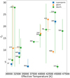 |
Fig. 4 Best-fit clumping factors from the GA, with ƒcl for supergiants shown by blue squares, orange triangles for giants, and green circles for dwarfs. We find weighted average values of ƒcl = 16 ± 1 and ƒcl = 7 ± 1 above and below 38 kK, respectively, with an overall average ƒcl = 11 ± 1 . For weak-wind stars, there are little to no wind signatures in the spectrum, and so ƒcl cannot be reliably determined with the current method. |
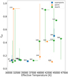 |
Fig. 5 Best-fit velocity filling factors from the GA, with ƒvel for super-giants shown by blue squares, orange triangles for giants, and green circles for dwarfs. We find average values of ƒvel = 0.44 ± 0.05 and ƒvel = 0.13 ± 0.04 above and below 38 kK, respectively. |
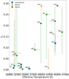 |
Fig. 6 Best-fit interclump density factors from the GA, with ƒic for supergiants shown by blue squares, orange triangles for giants, and green circles for dwarfs. We find average values of ƒic = 0.18 ± 0.04 and ƒic = 0.03 ± 0.04 above and below 38 kK, respectively. |
5.2.2 Weak-wind stars
For the four definite weak-wind stars (log(L/L⊙) < 5.0, VFTS517, VFTS280, VFTS235, and VFTS627), we find no constraint of ƒcl. It is well established that the optical features we rely on, such as Hα, are not sensitive to wind conditions at low  and that near-infrared and infrared diagnostics are required (Puls et al. 2006; Najarro et al. 2011). Additionally, UV lines are equally uncertain wind diagnostics at low
  if the X-ray properties of the star are not well constrained, although for two of the cooler stars (VFTS280 and VFTS223) we do find statistically significant constraints on the clumping factors, and in these cases the factors are low.
Simulations of the LDI in OB stars show that, for a relatively cool O-dwarf (~30 kK), the wind is less dense and comprises large shock-heated regions that are unable to cool, with increased ionisation resulting in lower UV line opacities, and thus the spectral appearance of a weak wind (Lagae et al. 2021). It may be that this process is also driving the lower clump filling in velocity space that we empirically find here.
Fundamentally, a low-velocity filling of high-density material means that more blue-shifted light in strong UV P-Cygni line profiles can escape, reducing absorption in the blue-shifted component of the P-Cygni profile and in extreme cases returning the feature to continuum levels. However, it might be that our low values of ƒvel are here actually mimicking the effects of a highly ionised bulk wind. Namely, if the bulk wind is hot and highly ionised at large velocities, there will be no remaining feature of the strong UV metal lines we rely on; the only signature available will be photospheric. This lack of wind features results in essentially the same spectral signature, in synthetic spectra, as no clump coverage, explaining the convergence to low values. Studies of the solar corona such as Mazzotta et al. (1998) predict carbon becoming rapidly ionised at temperatures greater than 106 K, while the LDI simulations of Lagae et al. (2021) find the average temperature of the wind to be at least 106 K, with large pockets of gas (spanning ≈0.1R*) reaching even higher temperatures. These profile morphologies and fitness distributions are consistent in all low-temperature dwarfs. There are no low-temperature giants to compare with. As for the three super-giants with low temperatures, we also find low-velocity filling, but there are clear P-Cygni profiles in these stars. The presence of wind features is to be expected in supergiants as the wind cooling is predicted to be much more efficient, meaning that the typical diagnostic lines remain and the wind signatures are still visible.
This change in wind feature morphology (from visible P-Cygni profiles to only absorption) corresponds well with similar studies of SMC dwarf stars. Bouret et al. (2013) notice this change in morphology around spectral type O6-7V at 38–40 kK, the only exception being AvZ 429 as an O7V star with wind features, although for this star there is no optical spectrum. In other studies of SMC dwarfs (Bouret et al. 2013; Bouret et al. 2021; Marcolino et al. 2022, and in our study), the models do not reproduce the strong absorption in C IV λλ1548–1551 in the near-photospheric profile. It is therefore unclear what is missing in the models to create this strong absorption at low velocity.
The lack of wind signatures in this context raises the question of whether the mass loss in weak-wind stars is truly as low as we measure here or whether we cannot constrain mass loss with the usual diagnostics. While the mass-loss rate cannot be high, as otherwise wind signatures would be observed, it is possible that the extremely low mass-loss rates allowed in the GA solutions are under-estimates. Previously, it was not computationally worthwhile to explore these extremely low mass-loss rate solutions, due to the lack of diagnostics in optical studies, and this is likely why we find statistically acceptable solutions down to the lowest end of the capabilities of the FASTWIND code and previous studies do not. It might be that the high degree of ionisation means we lose diagnostics in the UV and would need to search at even higher ionisation states in the FUV or X-rays. Indeed, some studies suggest weak-wind stars have been shown to host larger X-ray luminosities than giants and supergiants (Oskinova et al. 2006; Nebot Gómez-Morán & Oskinova 2018). Additionally, there is observational evidence that, when using X-ray diagnostics, the mass-loss rates determined for weak-wind stars are in good agreement with those found for typical main- sequence OB stars (Huenemoerder et al. 2012). This problem could also be alleviated with near-infrared and infrared observations, as the hydrogen Brackett series at these wavelengths is far more sensitive to wind physics, for stars with weak winds, than those in the optical (Najarro et al. 2011). The Brackett lines are also formed in close photospheric layers, and so might be relatively unaffected by the shock-heated outer wind. Or, it may be that the low density of these winds means that coupling between the accelerated metal ions and the abundant hydrogen and helium ions is no longer valid (Castor et al. 1976; Springmann & Pauldrach 1992; Babel 1996; Krticka & Kubát 2001; Owocki & Puls 2002), and so the mass-loss rates are actually capable of becoming as low as we observe in this sample.
5.3 Terminal wind speeds
For 12 of the stars in this sample, the P-Cygni profile of C IV λλ1548–1551 is strong enough to show extended blue- shifted absorption, from which we can easily diagnose the terminal wind speed. Six of the eight late-type subgiants and dwarfs (those with spectral types of O7 or later) do not have sufficient wind signatures to be able to measure a terminal wind speed using the diagnostics covered by observations used in this work. These parameters were left free in the GA fitting but our ability to constrain them is discussed on a case-by-case basis for the relevant stars in Appendix B. We compared the terminal wind from the GA to the value computed using the recipe provided in Hawcroft et al. (2023). These authors have derived a new empirical calibration for the terminal wind speed as a function of temperature and metallicity, based on an analysis of 150 OB stars in the LMC and SMC from the ULLYSES programme and the Galactic sample of Prinja et al. (1990). For nine of the 12 stars, we find good agreement between the calibration and GA results, within errors provided by the GA; four of these agree with the best-fit value within 100 km s−1 and the others generally have large errors on the terminal wind speed from the global fitness metric but the fitness distributions of C IV λλ1548–1551 peak closer to the prediction. The three stars in disagreement (VFTS440, VFTS385, and VFTS087) each seem to be discrepant for different reasons. VFTS087 has a much larger terminal wind speed than predicted from Hawcroft et al. (2023) and actually reaches the top of the parameter space in the GA, although it is possible that the main issue here is the normalisation in the UV as the GA fit to the bluest edge of the profile is poor. We can test this by directly measuring the velocity of maximum absorption in the P-Cygni trough. VFTS440 has a much better GA fit to C IV λλ1548–1551 but there is a secondary peak in the exploration between 2000 and 2100 km s−1 , close to the lower boundary. The prediction underestimates v∞ relative to the GA fit. Again, here it is useful to check with an alternate method. In VFTS385, we again have a good fit to a saturated profile, although there is some disagreement between the best-fit minimum χ2 and maximum fitness. This disagreement between fitness metrics is clearest in the temperature, as the maximum fitness is close to 40 kK, around 2 kK higher than the minimum χ2. Using 40 kK as an input to the prediction of Hawcroft et al. (2023) would increase v∞ by around 200 km s−1, bringing the discrepancy down to around 300 km s−1.
6 Conclusions
We have determined stellar and wind properties for a sample of 18 O-type stars in the LMC including dwarfs, giants, and supergiants with early to late spectral types. This was achieved through simultaneous spectroscopic fitting of UV and optical stellar and wind diagnostic line profiles using the code FASTWIND, optimised with a GA. Our main goal is to investigate the mass-loss rates and clumping properties of these stars. With this goal in mind, we have included the effects of optically thick clumping and clump coverage in velocity space. We find:
Well-defined empirical mass-loss rates that agree well with the theoretical predictions from Krtička & Kubát (2018) and Björklund et al. (2021) for stars within a luminosity range of 5.2 < log(L/L⊙) < 6.2, and agree best with the predictions from Krtička & Kubát (2018). These empirical rates are roughly four to five times lower than those predicted by Vink et al. (2001). This is a slightly larger discrepancy than the average scaling factors (around a factor of three) found in previous studies, which do not include the effects of optically thick clumping.
For dwarf-type stars with low luminosity, log(L/L⊙) < 5.2, mass-loss rates are orders of magnitude lower than predicted. This is attributed to the weak-wind problem. It is suggested that this discrepancy is due to shock-heating ionising metals used to diagnose wind properties, and so no discernible wind features remain in the UV spectra. Physical motivations for this are outlined in theoretical studies of the relatively low density winds of O dwarfs (Lucy 2012; Lagae et al. 2021). In this case, it is likely that mass-loss rates determined using typical UV diagnostics are lower limits. Generally, we find mass-loss rates lower than previous empirical studies as we explore lower mass-loss rate solutions. This is supported by our weak-wind mass-loss rates’ upper error limits approaching the lower estimates in the literature.
The strongest and most significant trend we find for the clumping factor with other stellar parameters is a positive correlation with the effective temperature. The average throughout the sample is found to be fcl = 11 ± 1. This depends somewhat on the luminosity class, due to the uneven distribution of stars throughout the effective temperature range available. The average is in agreement with theoretical predictions of the clumping factor for hot (∼40 kK) O-supergiants from 2D LDI simulations (Driessen et al. 2022). However, if we consider splitting the sample into hot stars (Teff > 38 kK) with typical winds (log(L/L⊙) > 5.2) and cooler weak-wind stars, we find f cl = 16 ± 1 and fcl = 7 ± 1, respectively.
For hot stars (Teff > 38 kK) with typical winds (log(L/L⊙) > 5.2), we find intermediate velocity filling factors, fvel = 0.44 ± 0.05 on average. This suggests that just under half of the wind velocity profile is covered by clumps. This is in good agreement with previous results for Galactic O-supergiants (Hawcroft et al. 2021) and for O stars in the LMC (Brands et al. 2022). For cooler weak-wind stars, the clump velocity filling converges to very low values (fvel = 0.13 ± 0.04), in an effort to fit the photospheric UV profiles that remain due to a lack of wind signatures. This indicates that either the wind is sufficiently porous to remove all high-velocity blue-shifted absorption, or that there is no diagnostic available due to the aforementioned wind ionisation.
A similar trend in interclump density as for velocity filling; hotter stars with typical winds have relatively larger interclump densities, around 20% of the mean wind density, similar to results for Galactic O-supergiants Hawcroft et al. (2021). For the cooler weak-wind stars, we find interclump densities approaching the lower limit of the parameter space, just a few percent or even lower than that of the mean wind (fic = 0.03 ± 0.04), although we note that this is related to the aforementioned issues in diagnosing the wind structure properties associated with optically thick clumping for weak-wind stars.
This analysis will be extended to lower metallicity as we measure stellar and wind properties for a similar sample in the SMC. We also await the full release of the optical follow-up to the HST-ULLYSES survey (Roman-Duval et al. 2020), X- Shooting ULLYSES. These surveys will together provide high- quality UV and optical spectra for more than 200 stars across the LMC and SMC (Vink et al. 2023; Sana et al. 2024). This will be an unprecedented opportunity to investigate the wind properties of massive, hot stars at low metallicity.
Data availability
Appendix C is available online at https://zenodo.org/records/13256608
Acknowledgements
We would like to thank the anonymous referee, for their helpful comments which improved the content and clarity of this paper.This project has received funding from the KU Leuven Research Council (grant C16/17/007: MAESTRO), the FWO through a FWO junior postdoctoral fellowship (No. 12ZY520N) as well as the European Space Agency (ESA) through the Belgian Federal Science Policy Office (BELSPO). LM thanks ESA and BELSPO for their support in the framework of the PRODEX programme (MAESTRO). The computational resources and services used in this work were provided by the VSC (Flemish Supercomputer Center), funded by the Research Foundation – Flanders (FWO) and the Flemish Government. This research has made use of the SIMBAD database, operated at CDS, Strasbourg, France.
Appendix A Best-fit stellar parameters
Appendix B Appendix - Star-by-Star
B.1 VFTS180
This star sits on the border of O-type supergiant and WR star but has been classed as O3 If* by Evans et al. (2011) and confirmed as apparently singe (Shenar et al. 2020). We find a well-defined temperature Teff = 44.1 ± 0.5 kK, 4 kK higher than Ramírez-Agudelo et al. (2017). The temperature in our fit is constrained primarily from the optical hydrogen and helium lines, although the He I lines are slightly too strong. The wings of the Balmer lines are reproduced very well to log g = 3.62 ± 0.05, and the higher temperature relative to Ramírez-Agudelo et al. (2017) is consistent with the log g we find which is 0.2 dex higher. However, it is difficult to compare the fits as the fit quality is deemed poor and left out of extended analysis of Ramírez-Agudelo et al. (2017). This is the most luminous star in our sample with log(L/L⊙) = 5.98 ± 0.07 and the highest mass-loss rate log(Ṁ[M⊙yr−1 ]) = −5.72 ± 0.05, thanks to the strong wind features this star also has some of the most well-defined fitness distributions. β is well constrained by the optical emission features to 1.2 ± 0.1 and v∞ is drawn towards an erroneously high value of 2650 km s−1, it should be closer to 2000 km s−1 from the saturated C IV λλ1548-1551 line. We find moderately low rotation of v sin i = 90 km s−1 and vmac = 50 km s−1, fairly consistent with Ramírez-Agudelo et al. (2017). We find a significant helium enrichment NHe/NH = 0.3, as do Ramírez-Agudelo et al. (2017) although the enrichment found in their study is higher, this is mainly constrained by the optical hydrogen and helium lines but the UV helium lines help as well. We find significant nitrogen enrichment from emission in the optical nitrogen lines, which are well fitted, at ϵ(N) = 8.93 ±0.1, essentially at the upper limit of our parameter space. Although there is emission in N V λ4603 which is not in the model. The wind parameters found for this star are consistent with those from Hawcroft et al. (2021) for Galactic O-type supergiants, suggesting the metallicity is not influencing these parameters much, at least for this star. The clumping factor is around 20, the velocity filling between 0.5 – 0.6, one-tenth average density in the interclump medium (ƒic = 0.12 ± 0.04) and the clumping onset is around 150 km s−1.
B.2 VFTS143
VFTS143 was determined to be O3.5V((fc)) by Walborn et al. (2014), indicating C III emission in the optical and absorption in He II λ4686. This star has not been included in previous atmosphere modelling studies but our derived Teff = 44.8 kK agrees with Walborn et al. (2014) within 0.1 kK and, with a log g = 3.9 ± 0.05, it sits within the parameter range of a typical O-dwarf in 30 Dor (Sabín-Sanjulián et al. 2017). It is also categorised as a large amplitude SB1 (Sana et al. 2013) and significant radial velocity variation can be seen in the GA best fit, mainly in the optical He II lines. The mass loss for this object lies comfortably in the trend for the full sample, and is well constrained by UV resonance lines e.g. C IV λλ1548-1551, although we find a very low clumping factor (fcl = 3 ± 3), with this low clumping constrained by optical lines such as Hα. The fitness distributions for fvel and fic are quite flat, reducing somewhat our confidence in the high values found of ∼ 0.7 and ∼ 0.3, respectively. This star is among those with the highest terminal wind speeds found in this sample, at 2900 km s−1 . The β value pushes to the upper edge of the parameter space, due to the Balmer series especially Hγ and Hδ. Rotation and macro- turbulent velocities are both moderate, near 100 km s−1. While we do not model the optical carbon features key to the spectral class of this object we do find a fairly standard carbon abundance for the LMC (Dopita et al. 2019; Brott et al. 2011a). From the GA fitness distributions it is difficult to say much about the oxygen abundance and nitrogen, they can be typical or depleted but certainly not enriched.
B.3 VFTS608
VFTS608 is an early-mid giant (O4III) only extensively studied in Bestenlehner et al. (2014). We find a temperature Teff = 43.0 ± 0.5 kK, which is 1kK higher than Bestenlehner et al. (2014) and fairly well constrained with a good optical fit, there are some issues due to significant line profile variability as identified in Sana et al. (2013), although the shift in e.g. the optical helium lines is not as severe as in VFTS143. The statistical significance of the line profile variability detection is similar between VFTS143 and VFTS608 but the magnitude of the variation is ∼40 km s−1 lower for VFTS608. The UV fit is not perfect but the main issue is that the Si IV λλ1394, 1403 lines are much too weak in our model, it appears the only way to reproduce these from the GA fitness distributions is to massively lower the temperature and or mass-loss rate. The surface gravity is well defined with a good fit (log g = 3.84 ± 0.05). The mass-loss rate is well constrained (log(Ṁ)= −6.24 ± 0.05) with a strong wind signature in C IV λλ1548-1551 but is lower than predicted, Björklund et al. (2021) over-predict the mass-loss rate by a factor 1.3. β is high, hitting the top of our parameter space at 2. Terminal wind speed is well constrained from C IV λλ1548-1551 to 2640 km s−1 which agrees with our prediction from Hawcroft et al. (2023). The clumping factor is well constrained (fcl = 9 ± 1) from the optical and, along with VFTS143 is one of the two stars with a low clumping factor and relatively high temperature, although much of the Hα core had to be removed. The velocity filling is at the lower bound fvel ∼ 0.1 and the interclump density is intermediate fic ∼ 0.15 , both appearing to be mainly constrained by C IV λλ1548-1551 and He II λ4686. Rotation is normal with unconstrained macro. Helium abundance is normal, only slightly higher than most of the sample. Nitrogen is well constrained and enriched, carbon is maybe depleted and oxygen is lower than baseline2.
B.4 VFTS216
VFTS216 is an early-type dwarf (O4V) with fairly strong wind signatures in the UV. It was previously studied by Sabín-Sanjulián et al. (2017). We obtain a very good fit, aside from issues with normalisation around the N III λλ-4634-4640-4642 lines, resulting in a temperature ( and log g = 3.74 ± 0.05, which agree well with Sabín-Sanjulián et al. (2017). Ṁ, β and v∞ are fairly well constrained, Ṁ is half that predicted by Björklund et al. (2021), β is quite high at 1.6 ± 0.2 and v∞ agrees well with our predictions. The clumping factors are not very well constrained, fcl ∼ 9 – 26, fvel ∼ 0.25 – 1.0 and fic ∼ 0.06 – 0.28, so it is difficult to comment on these parameters for this star. Rotation and macroturbulence velocities are moderate, around 100 km s−1 and 80 km s−1, respectively. The helium abundance is normal. The nitrogen abundance is baseline and well constrained. The carbon abundance is fairly typical, the error bars including both baseline values, and oxygen also appears to be baseline.
B.5 VFTS184
VFTS184 is mid-late type dwarf (O6.5V) which is just on the edge of the weak-wind regime and has not been previously analysed. We obtain a good fit in the optical but the fit is not as good in the UV, for example the C IV λλ1548-1551 line which has an unusual morphology. The mass-loss rate hit the lower boundary of our fitting range so we launched another run, finding that the mass-loss rate is fairly well defined at log(Ṁ)= −8.45 ± 0.15, a factor of 2 lower than predicted by Björklund et al. (2021). This star is also a relatively fast rotator with v sin i ∼ 350 km s−1. β is typical (∼1.1) but is not well peaked, the same can be said for v∞, which has a flat fitness distribution along with a poor fit to C IV λλ1548-1551 but the value found agrees with a direct measurement and our predictions. The fitness distributions for the clumping parameters are quite flat but with good constraints fcl ∼ 16 ± 5, fvel ∼ 0.35 ± 0.05 and fic ∼ 0.1 ± 0.1. Normal helium abundance. Low to standard nitrogen and carbon abundances with oxygen again not present in the UV and unconstrained.
B.6 VFTS244
VFTS244 is a mid O-type giant (O5III) also modelled by Ramírez-Agudelo et al. (2017). We find a temperature 1 kK lower and surface gravity 0.1 dex lower than Ramírez-Agudelo et al. (2017) which is fair agreement (Teff = 39.7 ± 0.5 kK and log g = 3.58 ± 0.05). The fit quality is high, there are some issues in fitting the Si IV λλ1394, 1403 lines and matching the strength of the absorption in He II λ4686. We also have to remove the core of Hα. Our mass-loss rate (log(Ṁ)= −6.40 ± 0.05) is lower than Ramírez-Agudelo et al. (2017), with the same luminosity, so this discrepancy seems to be due to the inclusion of clumping, after correction the mass-loss rates are in agreement. Our mass-loss rate is double that of the prediction from Björklund et al. (2021) and 4.5 times lower than the prediction of Vink et al. (2001). We have a good constraint on the terminal wind speed from a saturated C IV λλ1548-1551 profile, we find v∞ = 2550 km s−1 which is around 300 km s−1 higher than our prediction. β converges to the upper limit of the parameter space around a value of 2.0, driven by the optical hydrogen lines. The clumping factor (fcl = 16 ~ 20) is close to that found for Galactic O-supergiants (Hawcroft et al. 2021), and also well constrained by optical hydrogen. It is generally difficult to disentangle the effects of velocity filling and interclump density, though here we find that fvel(= 0.15 ~ 1.0) is unconstrained and fic(= 0.22 ~ 0.3) must be high. This star has is one of the highest rotation rates in this sample (v sin i = 200 – 250 km s−1) which agrees with the findings of Ramírez-Agudelo et al. (2017). Helium abundance is normal. It appears nitrogen is slightly enhanced and carbon depleted. Oxygen looks normal, but maybe slightly lower than baseline.
B.7 VFTS664
VFTS664 is a mid-late bright giant (O7II) and is also included in Ramírez-Agudelo et al. (2017). The fit is not bad but not as good as most of the stars in this sample, mainly the fits to C IV λλ1548-1551 and Si IV λλ1394, 1403 are poor, and the cores of all the optical hydrogen lines are lost to nebular contamination. We find good agreement with Ramírez-Agudelo et al. (2017) in temperature and surface gravity. C IV λλ1548-1551 is the only line with a clear wind signature, but the mass-loss rate is well constrained and found to be a factor 3.4 lower than the prediction of Vink et al. (2001) and a factor 2.6 larger than the prediction of Björklund et al. (2021). β is fairly high, between 1.6–1.9, and terminal wind speed is hard to determine due to the very low gradient of the blue edge. Interestingly, the clumping factor is decidedly low fcl = 3 ~ 6, and the velocity filling and interclump density converge to the lower bound of the parameter space, fvel ∼ 0.1 and fic ∼ 0.01. Rotation is again moderate, close to 100 km s−1 with a matching macroturbulence. Nitrogen is enriched with typical carbon. Oxygen is not well constrained and the helium abundance is normal.
B.8 VFTS087
VFTS087 is a (super/bright-)giant (O9.7I-II), and is also included in Ramírez-Agudelo et al. (2017). The fit to the optical spectrum is very good, aside from a few metal lines, in the UV we may have some issues with normalistion that could be affecting the fit. We find this star to have the lowest temperature in our sample Teff = 31.0 ± 0.5 kK and log g = 3.35 ± 0.05, in very good agreement with Ramírez-Agudelo et al. (2017). The terminal wind speed is found to be very high as discussed in Sect. 5.3, perhaps due to normalisation or related to the high β (= 3.0 ± 0.7), the fitness distribution of which peaks below 1.0 in the fit to C IV λλ1548-1551. The mass-loss rate is constrained mainly by the optical hydrogen lines in this fit, and with log(Ṁ)= −6.75 ± 0.05 it lies between predictions, a factor 2 lower than Vink et al. (2001) and a factor 5 higher than Björklund et al. (2021). All clumping properties are towards the lower limits (fcl = 4 ± 1, fvel = 0.17 ± 0.05 and fic = 0.01 ± 0.05). The clumping factor is strongly constrained by the optical hydrogen lines, and the nebular contamination is not too bad in this star so most of the cores remain. The velocity filling and interclump density factors are strongly constrained by the UV, in particular the Si IV λλ1394, 1403 lines. Part of the fitting region of these lines is signficantly above the continuum but the morphology is unusual (see Fig. C.13), if there is no emission component and this morphology is only due to issues with normalisation, it is hard to say what effect this would have on the parameters but they may change. Rotation is well constrained as moderate to low, and the macroturbulence is similar, 70 ± 10 km s−1 and 30 ± 10 km s−1 . The helium abundance is normal, nitrogen is clearly enriched, nitrogen and carbon are well constrained. Carbon and oxygen abundances seem normal.
B.9 VFTS440
VFTS440 is a mid-type bright giant (O6-6.5II), and is also included in Ramírez-Agudelo et al. (2017). The fit is interesting as there is disagreement between best-fit values between the optical hydrogen lines while much of the core and red-wings must be removed, we also have issues fitting Si IV λλ1394, 1403, O IV λλ1340-1344 and He II λ4686. There could also be issues due to binarity as this star is flagged as an SB1 in Almeida et al. (2017). The temperature and surface gravity (Teff = 33.4 ± 0.5 kK and log g = 3.13 ± 0.05) are consistent with Ramírez-Agudelo et al. (2017) but both are heavily constrained by Hα and the He II lines. Looking at the fitness distributions for the other Balmer lines and some He I lines, they mostly peak towards another solution with log g ~ 3.7 and Teff ~ 40 kK. The terminal wind speed could be lower, as discussed in Sect 5.3. β (∼ 1.6) is fairly high, again constrained by optical hydrogen. The mass-loss rate (log(Ṁ)= −6.23 ± 0.05) is well constrained by the optical, and the fit to UV is not bad, it is a factor 4 lower than Vink et al. (2001) and a factor 2 higher than Björklund et al. (2021). The clumping factors again are low (fcl = 9 ± 1, fvel = 0.14 ± 0.05 and ƒic = 0.02 ± 0.05), with some possible secondary peak at fcl ~ 15 in Hα. The velocity filling and interclump density factors are low although it is not clear that any lines in particular are driving this, and here the normalisation is good unlike VFTS087. Again we find fairly standard broadening for this sample. Helium, nitrogen and carbon abundances are well constrained. Helium is normal to slightly high. We find significant nitrogen enrichment, while the carbon abundance is normal. Oxygen abundance is normal but the O IV λλ1340-1344 lines are clearly underestimated in our fit.
B.10 VFTS385
VFTS385 is a mid O-type dwarf (O4-5V) also modelled by Sabín-Sanjulián et al. (2017). We find a temperature and surface gravity lower (2 kK and 0.25 dex) than Sabín-Sanjulián et al. (2017) (Teff = 37.7 – 39.1 kK and log g = 3.55 ± 0.05). The fit quality is high, although there are some issues in fitting the Si IV λλ1394, 1403 lines and we remove the cores of the Balmer lines. Our mass-loss rate (log(Ṁ)= −6.29 ± 0.05) is a factor 1.6 lower than the Vink et al. (2001) prediction and a factor 9.8 higher than the prediction from Björklund et al. (2021). There is some discrepancy in the terminal wind speed, discussed in Sect. 5.3. β is found to be between 0.6 – 0.7, which is a bit low. The clumping factor distribution is not very well defined but we find fcl = 13 ± 1. We find a fairly low velocity filling factor fvel(= 0.13 ± 0.05) and fairly typical interclump density (fic = 0.10 ± 0.05). Rotation and macroturbulence velocities are moderate, around 120 km s−1 and 90 km s−1 , respectively. The helium abundance is normal. It appears that the nitrogen and carbon abundances are baseline to slightly reduced and oxygen is enhanced, converging to the upper limit of our parameter space.
B.11 VFTS096
VFTS096 is a mid O-type dwarf (O6V) and is included in Sabín-Sanjulián et al. (2017). The fit is good, although there are issues fitting the carbon lines, and the fitness distributions are very flat with a number of unconstrained parameters. Our best fit temperature and surface gravity agree well with Sabín-Sanjulián et al. (2017) and at least the surface gravity is well defined by the Balmer lines, ( and log g = 3.90 ± 0.1). Terminal wind speed is low here, with v∞ ∼ 2300 km s−1, which agrees with the predictions of Hawcroft et al. (2023) v∞ ∼ 2400 km s−1 but could actually be close to 2800 km s−1 from the C IV λλ1548- 1551 line. β is high (1.5 ± 0.5), which is consistent with other O dwarfs due to optical hydrogen, but with a large range the typical value is included. Mass-loss rate has a strong upper limit of log(Ṁ)∼ −6.5, and less strong lower limit at log(Ṁ)∼ −7.0, very low compared to theoretical predictions, a factor 12 lower than Vink et al. (2001) and a factor 6 lower than Björklund et al. (2021) in the worst case and a factor 5 and 2 lower in at the upper limit of Ṁ. There is only a wind signature in C IV λλ1548- 1551 which has a fairly atypical morphology, it is difficult to constrain any wind parameters within the large range of massloss rates available, and the error margins encompass almost the full parameter space for clumping factor, interclump density and velocity filling. Rotation is typical and moderate (v sin i ∼ 90 - 140 km s−1 ), with macroturbulence unconstrained. The helium, nitrogen and carbon abundances have some of the more well constrained fitness distributions. Helium abundance is typical. Carbon is typical to low and converges to the lower limit of the parameter space. Nitrogen features are very weak, with a low nitrogen abundance, again towards the lower edge of the parameter space. Oxygen is unconstrained but UV diagnostics peak in fitness around LMC baseline or slightly higher.
B.12 VFTS586
VFTS586 is an earlier O-type dwarf (O4V) and is included in Sabín-Sanjulián et al. (2017). For this star we achieve a high quality fit to all lines apart from Si IV λλ1394, 1403, and Sabín-Sanjulián et al. (2017) also have a good optical fit. The hydrogen line cores are removed but most of the wings remain. We find a well constrained temperature and surface gravity 1 kK higher and 0.1 dex lower than Sabín-Sanjulián et al. (2017) with Teff = 46.2 ± 0.5 kK and log g = 3.90 ± 0.05. Terminal wind speed is well constrained by C IV λλ1548-1551 and agrees very well with our prediction. A high β(= 1.5 ± 0.1) results from the optical hydrogen lines while the UV diagnostics tend to prefer a lower beta. A strong upper limit is placed on the mass-loss rate (log(Ṁ)= −6.85 ± 0.07) by the optical hydrogen and helium lines and the peak agrees well with UV diagnostics. This Ṁ is a factor 9.5 lower than predicted by Vink et al. (2001) and a factor 1.7 higher than Björklund et al. (2021). The clumping factor cannot be too high or too low, fcl ∼ 15 ± 5. The velocity filling factor is in the lower half of the parameter space and interclump density is not well constrained but must be fairly high (fvel(= 0.30 ± 0.15), fic ∼ 0.07 – 0.28). Rotation is typical and moderate (v sin i ∼ 80 – 100 km s−1), with macroturbulence unconstrained. All the abundances are well constrained. Helium abundance is typical, carbon is very consistent with LMC baseline, nitrogen is maybe low and the features are very weak. Oxygen abundance is high due to strong UV optical features.
B.13 VFTS422
With Teff = 42kK and log g = 3.5, VFTS422 star is an early-mid giant (O4III). Although the fit is not very good due to relatively low S/N and we have to remove the hydrogen line cores and fairly significant parts of the wings due to nebular contamination and exclude Hα. As a result the fitness distributions are fairly flat and the peaks in surface gravity and mass-loss rate are not in great agreement with the best fit. It could be that our surface gravity is up to 0.3 dex too low which would also impose a significant upper bound on the effective temperature. This star is included in the sample of Bestenlehner et al. (2014), who find a comparatively low Teff = 40kK, although these authors use the optical nitrogen lines to determine Teff and we would likely see a reduction in our best fit value if our focus was shifted to these lines. There are again a number of issues with radial velocity typical of a large amplitude SB1, as confirmed by Sana et al. (2013). This star has fairly high rotation at 200 km s−1, although this is significantly lower than the 356 km s−1 reported in Bestenlehner et al. (2014). Again the nebular contamination and radial velocity variation can affect this. The largest discrepancy comes when comparing the mass-loss from the GA and Bestenlehner et al. (2014) which find −6.48 and −5.6 respectively. Bestenlehner et al. (2014) include a modest clumping correction but still reproduce a mass-loss rate close to the Vink et al. (2001) prediction. We find the clumping factor to be similar to that found for Galactic O-supergiants, fcl ∼ 21 ± 3. Note that we find a luminosity matching exactly that of Bestenlehner et al. (2014) and a mass-loss rate in very good agreement with the prediction of Björklund et al. (2021). We find a terminal wind speed of 2100 km s−1 which is 300 km s−1 lower than our prediction and nearly 700 kms−1 lower than Bestenlehner et al. (2014), although these authors calibrate this from an overall wind strength due to a lack of UV diagnostics. It is also worth noting the decidedly low β value in our best fit, perhaps due to the difficulty in obtaining a high quality fit to the optical, a low beta, as is commonly preferred in the UV, is converged upon. Despite issues in the optical, the fit quality is higher in the UV, the main issue is fitting Si IV λλ1394, 1403. We find fairly low velocity filling and interclump density factors ( fvel ∼ 0.4, although the fitness distribution peaks towards the lower end, mostly due to N IV λ1718 so this could be an upper limit, and fic ∼ 0.01 – 0.10) We find normal to low helium abundance, significant carbon and nitrogen enhancements compared to the LMC baseline and oxygen depletion.
B.14 VFTS627
VFTS627 is the latest type O dwarf in our sample (O9.7V) and a weak-wind star, also included in Sabín-Sanjulián et al. (2017). We are able to obtain a very high quality fit for all lines, except for C IV λλ1548-1551, the strength of the absorption is underestimated in this line, as is common for weak-wind stars. The fit to the optical in Sabín-Sanjulián et al. (2017) is also very good. Although we find a temperature 2 kK lower which is highly constrained by UV lines, which may also help to explain our 0.35 dex lower surface gravity (Teff = 30.5 – 32.0 kK and log g = 3.70 – 3.85). Although the difference in wind parameters may also contribute here, we can see that we have much stronger absorption in Hα, which is hard to confirm as the Balmer line cores are removed but more of the core remains in the higher level Balmer lines, the strength of which are matched well. There is no diagnostic for the terminal wind speed and essentially no constraint for β, the fitness distributions are very flat. We find a mass-loss rate of log(Ṁ)= −10.5 ± 0.1, the lowest in the sample and very related to the weak-wind problem (see discussion in Sect. 5.2.2). There is no constraint on any of the clumping factors. Rotation is low (v sin i < 80 kms−1 ) and macroturbulence fairly high (vmac = 85 ± 10 km s−1). Helium, nitrogen and carbon abundances are well constrained while oxygen is not, with little to no visible diagnostics. Helium abundance is normal. Carbon abundance is typical for the LMC, nitrogen may be a bit high as found by N III λλ-4634-4640-4642.
B.15 VFTS280
VFTS280 is a late O dwarf (O9V) and is another weak-wind star, also included in Sabín-Sanjulián et al. (2017). The fit is quite good, especially in the optical, except of course to C IV λλ1548-1551. We find very well constrained temperature and surface gravity, consistent with Sabín-Sanjulián et al. (2017) at (Teff = 33.4 ± 0.5 kK and log g = 3.76 ± 0.05). β and v∞ are low but fairly unconstrained due to lack of diagnostics. Mass-loss rate is low  . Clumping factor is essentially unconstrained ( fcl ∼ 4 – 19), it just cannot be high. Here the velocity filling and interclump density factor converge to the lower bound of the parameter space due to C IV λλ1548-1551 (see discussion in Sect. 5.2.2). Rotation is a bit higher (v sin i = 155 ± 20 km s−1) and the macroturbulence is fairly high (vmac = 90 ± 5 km s−1 ). All abundances apart from oxygen are fairly well constrained and normal.
B.16 VFTS235
VFTS235 is a very late O giant (O9.7II) and is included in Ramírez-Agudelo et al. (2017). All of our findings are very close to VFTS627. The fit here is very good, even the C IV λλ1548-1551 absorption strength is fairly close. We have well defined temperature and surface gravity peaks in full agreement with Ramírez-Agudelo et al. (2017) at (Teff = 32.5 ± 1.0 kK and log g = 4.2 ± 0.1) but the surface gravity is the highest in the sample, higher than all the stars classed as dwarfs. Again there is no diagnostic for the terminal wind speed or β so these parameters are completely unconstrained. The mass-loss rate converges to the lowest capabilities of FASTWIND, with only an upper bound constrained log(Ṁ)< −10.0. Again there is no constraint on any of the clumping factors. Rotation is low (v sin i < 50 km s−1) and macroturbulence is moderate (vmac = 50 ± 20 km s−1 ). Helium abundance is normal. Nitrogen abundance is low in our best fit but with large error bars, from the spectrum it appears the nitrogen abundance should be closer to our upper error limit, around 7.5 which is in good agreement with Grin et al. (2017). A bit higher than LMC baseline around 6.9–7.2. Carbon abundance is low but may actually be close to baseline if we were to focus on CIII lines in the UV. Oxygen is not constrained and it is difficult to distinguish features in the UV.
B.17 VFTS223
VFTS223 is a late sub-giant star (O9.5IV), also included in Sabín-Sanjulián et al. (2017) and has very similar spectral morphology as the weak-wind stars. Again the fit is very good, temperature and surface gravity are well constrained (Teff = 33.8 ± 0.5 kK and log g = 3.86 ± 0.05) and both are significantly lower than Sabín-Sanjulián et al. (2017). Terminal wind speed and β are similar to other weak-wind stars, there is little to no diagnostic and these parameters are essentially unconstrained. Perhaps some wind is seen in C IV λλ1548-1551, and the mass-loss rate is actually constrained to log(Ṁ)= −7.6 ± 0.25. Clumping factor cannot be too high ( fcl ∼ 11 ± 4). Much like VFTS280, the velocity filling and interclump density factor converge to the lower bound of the parameter space due to C IV λλ1548-1551 (again see discussion in Sect. 5.2.2). Rotation is very low (v sin i < 13 km s−1 ) and macroturbulence is moderate (vmac ∼ 60km s−1 ). All abundances have some constraint, the metal lines are generally clear and well fitted giving well peaked fitness distributions for carbon and nitrogen but oxygen is not clear in the UV so that is low and fairly unconstrained. We find a normal helium abundance and nitrogen is typical to slightly enhanced, carbon is typical to slightly depleted.
B.18 VFTS517
VFTS517 is a late O dwarf/giant (O9.5V-III), appears to be another weak-wind star and is included in Sabín-Sanjulián et al. (2017). We find significantly lower temperature and surface gravity than Sabín-Sanjulián et al. (2017), much like for VFTS223 (Teff = 31.2 ± 0.5 kK and log g = 3.67 ± 0.07) but we have high quality fits and well peaked fitness distributions for these parameters. Further repetition for the terminal wind speed and β, there is little to no diagnostic and these parameters are essentially unconstrained. The mass-loss rate converges to the lowest capabilities of FASTWIND, with only an upper bound constrained log(Ṁ)< −9.7, although Hα could be fitted with a higher mass-loss rate, which disagrees with all other diagnostics. There is no constraint on the clumping factor, and the velocity filling factors are slightly better constrained but essentially only offer upper limits (fvel < 0.4, fic < 0.23). Rotation is moderate (v sin i = 100 ± 50 km s−1) and the macroturbulence is unconstrained. Again all abundances have some constraint. The helium abundance is normal. Nitrogen may be slightly increased from baseline, but carbon is typical, oxygen is fairly absent from the spectrum so either depleted or unconstrained.
References
- Abdul-Masih, M., Sana, H., Sundqvist, J., et al. 2019, ApJ, 880, 115 [Google Scholar]
- Abdul-Masih, M., Sana, H., Hawcroft, C., et al. 2021, A&A, 651, A96 [NASA ADS] [CrossRef] [EDP Sciences] [Google Scholar]
- Almeida, L. A., Sana, H., Taylor, W., et al. 2017, A&A, 598, A84 [NASA ADS] [CrossRef] [EDP Sciences] [Google Scholar]
- Anders, E., & Grevesse, N. 1989, Geochim. Cosmochim. Acta, 53, 197 [Google Scholar]
- Asplund, M., Grevesse, N., Sauval, A. J., & Scott, P. 2009, ARA&A, 47, 481 [NASA ADS] [CrossRef] [Google Scholar]
- Babel, J. 1996, A&A, 309, 867 [Google Scholar]
- Bestenlehner, J. M., Gräfener, G., Vink, J. S., et al. 2014, The VLT-FLAMES tarantula survey: XVII. Physical and wind properties of massive stars at the top of the main sequence [Google Scholar]
- Björklund, R., Sundqvist, J. O., Puls, J., & Najarro, F. 2021, A&A, 648, A36 [EDP Sciences] [Google Scholar]
- Björklund, R., Sundqvist, J. O., Singh, S. M., Puls, J., & Najarro, F. 2023, A&A, 676, A109 [NASA ADS] [CrossRef] [EDP Sciences] [Google Scholar]
- Bouret, J. C., Lanz, T., Hillier, D. J., et al. 2003, ApJ, 595, 1182 [NASA ADS] [CrossRef] [Google Scholar]
- Bouret, J. C., Lanz, T., & Hillier, D. J. 2005, A&A, 438, 301 [NASA ADS] [CrossRef] [EDP Sciences] [Google Scholar]
- Bouret, J. C., Hillier, D. J., Lanz, T., & Fullerton, A. W. 2012, A&A, 544, A67 [NASA ADS] [CrossRef] [EDP Sciences] [Google Scholar]
- Bouret, J. C., Lanz, T., Martins, F., et al. 2013, A&A, 555, A1 [NASA ADS] [CrossRef] [EDP Sciences] [Google Scholar]
- Bouret, J. C., Martins, F., Hillier, D. J., et al. 2021, A&A, 647, A134 [NASA ADS] [CrossRef] [EDP Sciences] [Google Scholar]
- Brands, S. A., de Koter, A., Bestenlehner, J. M., et al. 2022, A&A, 663, A36 [Google Scholar]
- Brott, I., de Mink, S. E., Cantiello, M., et al. 2011a, A&A, 530, A115 [NASA ADS] [CrossRef] [EDP Sciences] [Google Scholar]
- Brott, I., Evans, C. J., Hunter, I., et al. 2011b, A&A, 530, A116 [NASA ADS] [CrossRef] [EDP Sciences] [Google Scholar]
- Carlberg, R. G. 1980, ApJ, 241, 1131 [Google Scholar]
- Carneiro, L. P., Puls, J., Sundqvist, J. O., & Hoffmann, T. L. 2016, A&A, 590, A88 [NASA ADS] [CrossRef] [EDP Sciences] [Google Scholar]
- Castor, J. I., Abbott, D. C., & Klein, R. I. 1975, ApJ, 195, 157 [Google Scholar]
- Castor, J. I., Abbott, D. C., & Klein, R. I. 1976, in Physique des Mouvements dans les Atmospheres, eds. R. Cayrel, & M. Steinberg, 363 [Google Scholar]
- Charbonneau, P. 1995, ApJS, 101, 309 [Google Scholar]
- Cohen, D. H., Wollman, E. E., Leutenegger, M. A., et al. 2014, MNRAS, 439, 908 [NASA ADS] [CrossRef] [Google Scholar]
- Crowther, P. A., Hillier, D. J., Evans, C. J., et al. 2002, ApJ, 579, 774 [Google Scholar]
- de Almeida, E. S. G., Marcolino, W. L. F., Bouret, J. C., & Pereira, C. B. 2019, A&A, 628, A36 [NASA ADS] [CrossRef] [EDP Sciences] [Google Scholar]
- Dessart, L., & Owocki, S. P. 2003, A&A, 406, L1 [NASA ADS] [CrossRef] [EDP Sciences] [Google Scholar]
- Dopita, M. A., Seitenzahl, I. R., Sutherland, R. S., et al. 2019, AJ, 157, 50 [Google Scholar]
- Driessen, F. A., Sundqvist, J. O., & Kee, N. D. 2019, A&A, 631, A172 [NASA ADS] [CrossRef] [EDP Sciences] [Google Scholar]
- Driessen, F. A., Sundqvist, J. O., & Dagore, A. 2022, A&A, 663, A40 [NASA ADS] [CrossRef] [EDP Sciences] [Google Scholar]
- Eggenberger, P., Ekström, S., Georgy, C., et al. 2021, A&A, 652, A137 [NASA ADS] [CrossRef] [EDP Sciences] [Google Scholar]
- Evans, C. J., Lennon, D. J., Trundle, C., Heap, S. R., & Lindler, D. J. 2004, ApJ, 607, 451 [NASA ADS] [CrossRef] [Google Scholar]
- Evans, C. J., Taylor, W. D., Hénault-Brunet, V., et al. 2011, A&A, 530, A108 [NASA ADS] [CrossRef] [EDP Sciences] [Google Scholar]
- Eversberg, T., Lépine, S., & Moffat, A. F. J. 1998, ApJ, 494, 799 [NASA ADS] [CrossRef] [Google Scholar]
- Fabry, M., Hawcroft, C., Frost, A. J., et al. 2021, A&A, 651, A119 [NASA ADS] [CrossRef] [EDP Sciences] [Google Scholar]
- Feldmeier, A. 1995, A&A, 299, 523 [NASA ADS] [Google Scholar]
- Fullerton, A. W., Massa, D. L., & Prinja, R. K. 2006, ApJ, 637, 1025 [Google Scholar]
- Georgy, C., Ekström, S., Eggenberger, P., et al. 2013, A&A, 558, A103 [NASA ADS] [CrossRef] [EDP Sciences] [Google Scholar]
- Gibson, B. K. 2000, Mem. Soc. Astron. Italiana, 71, 693 [NASA ADS] [Google Scholar]
- Gräfener, G., & Hamann, W. R. 2008, A&A, 482, 945 [Google Scholar]
- Gräfener, G., Koesterke, L., & Hamann, W. R. 2002, A&A, 387, 244 [NASA ADS] [CrossRef] [EDP Sciences] [Google Scholar]
- Grin, N. J., Ramírez-Agudelo, O. H., de Koter, A., et al. 2017, A&A, 600, A82 [NASA ADS] [CrossRef] [EDP Sciences] [Google Scholar]
- Groh, J. H., Ekström, S., Georgy, C., et al. 2019, A&A, 627, A24 [NASA ADS] [CrossRef] [EDP Sciences] [Google Scholar]
- Hawcroft, C., Sana, H., Mahy, L., et al. 2021, A&A, 655, A67 [NASA ADS] [CrossRef] [EDP Sciences] [Google Scholar]
- Hawcroft, C., Sana, H., Mahy, L., et al. 2023, A&A, 688, A105 [Google Scholar]
- Hillier, D. J., & Miller, D. L. 1998, ApJ, 496, 407 [NASA ADS] [CrossRef] [Google Scholar]
- Hillier, D. J., Lanz, T., Heap, S. R., et al. 2003, ApJ, 588, 1039 [Google Scholar]
- Huenemoerder, D. P., Oskinova, L. M., Ignace, R., et al. 2012, ApJ, 756, L34 [Google Scholar]
- Hunter, I., Brott, I., Langer, N., et al. 2009, A&A, 496, 841 [NASA ADS] [CrossRef] [EDP Sciences] [Google Scholar]
- Jiang, Y.-F., Cantiello, M., Bildsten, L., et al. 2018, Nature, 561, 498 [NASA ADS] [CrossRef] [Google Scholar]
- Johnston, C., Aimar, N., Abdul-Masih, M., et al. 2021, MNRAS, 503, 1124 [NASA ADS] [CrossRef] [Google Scholar]
- Kato, D., Nagashima, C., Nagayama, T., et al. 2007, PASJ, 59, 615 [NASA ADS] [Google Scholar]
- Keszthelyi, Z., Puls, J., & Wade, G. A. 2017, A&A, 598, A4 [NASA ADS] [CrossRef] [EDP Sciences] [Google Scholar]
- Köhler, K., Langer, N., de Koter, A., et al. 2015, A&A, 573, A71 [NASA ADS] [CrossRef] [EDP Sciences] [Google Scholar]
- Krticka, J., & Kubát, J. 2001, A&A, 377, 175 [NASA ADS] [CrossRef] [EDP Sciences] [Google Scholar]
- Krticka, J., & Kubát, J. 2018, A&A, 612, A20 [NASA ADS] [CrossRef] [EDP Sciences] [Google Scholar]
- Kurt, C. M., & Dufour, R. J. 1998, in Revista Mexicana de Astronomia y Astrofisica Conference Series, 7, eds. R. J. Dufour, & S. Torres-Peimbert, 202 [NASA ADS] [Google Scholar]
- Lagae, C., Driessen, F. A., Hennicker, L., Kee, N. D., & Sundqvist, J. O. 2021, A&A, 648, A94 [NASA ADS] [CrossRef] [EDP Sciences] [Google Scholar]
- Langer, N. 2012, ARA&A, 50, 107 [CrossRef] [Google Scholar]
- Lépine, S., & Moffat, A. F. J. 2008, AJ, 136, 548 [CrossRef] [Google Scholar]
- Lucy, L. B. 2012, A&A, 544, A120 [NASA ADS] [CrossRef] [EDP Sciences] [Google Scholar]
- MacGregor, K. B., Hartmann, L., & Raymond, J. C. 1979, ApJ, 231, 514 [Google Scholar]
- Mahy, L., Rauw, G., De Becker, M., Eenens, P., & Flores, C. A. 2015, A&A, 577, A23 [NASA ADS] [CrossRef] [EDP Sciences] [Google Scholar]
- Marchenko, S. V., Foellmi, C., Moffat, A. F. J., et al. 2007, ApJ, 656, L77 [NASA ADS] [CrossRef] [Google Scholar]
- Marcolino, W. L. F., Bouret, J. C., Martins, F., et al. 2009, A&A, 498, 837 [NASA ADS] [CrossRef] [EDP Sciences] [Google Scholar]
- Marcolino, W. L. F., Bouret, J. C., Rocha-Pinto, H. J., Bernini-Peron, M., & Vink, J. S. 2022, MNRAS, 511, 5104 [NASA ADS] [CrossRef] [Google Scholar]
- Markova, N., Puls, J., Dufton, P. L., et al. 2020, A&A, 634, A16 [NASA ADS] [CrossRef] [EDP Sciences] [Google Scholar]
- Martins, F., Schaerer, D., Hillier, D. J., & Heydari-Malayeri, M. 2004, A&A, 420, 1087 [NASA ADS] [CrossRef] [EDP Sciences] [Google Scholar]
- Martins, F., Schaerer, D., Hillier, D. J., et al. 2005, A&A, 441, 735 [NASA ADS] [CrossRef] [EDP Sciences] [Google Scholar]
- Massa, D., Fullerton, A. W., Sonneborn, G., & Hutchings, J. B. 2003, ApJ, 586, 996 [NASA ADS] [CrossRef] [Google Scholar]
- Mazzotta, P., Mazzitelli, G., Colafrancesco, S., & Vittorio, N. 1998, A&AS, 133, 403 [NASA ADS] [CrossRef] [EDP Sciences] [Google Scholar]
- Moens, N., Poniatowski, L. G., Hennicker, L., et al. 2022, A&A, 665, A42 [NASA ADS] [CrossRef] [EDP Sciences] [Google Scholar]
- Mokiem, M. R., De Koter, A., Puls, J., et al. 2005, A&A, 441, 711 [NASA ADS] [CrossRef] [EDP Sciences] [Google Scholar]
- Mokiem, M. R., De Koter, A., Evans, C. J., et al. 2006, A&A, 456, 1131 [NASA ADS] [CrossRef] [EDP Sciences] [Google Scholar]
- Mokiem, M. R., de Koter, A., Vink, J. S., et al. 2007, A&A, 473, 603 [NASA ADS] [CrossRef] [EDP Sciences] [Google Scholar]
- Muijres, L. E., de Koter, A., Vink, J. S., et al. 2011, A&A, 526, A32 [NASA ADS] [CrossRef] [EDP Sciences] [Google Scholar]
- Murphy, L. J., Groh, J. H., Ekström, S., et al. 2021, MNRAS, 501, 2745 [NASA ADS] [CrossRef] [Google Scholar]
- Najarro, F., Hanson, M. M., & Puls, J. 2011, A&A, 535, A32 [NASA ADS] [CrossRef] [EDP Sciences] [Google Scholar]
- Nebot Gómez-Morán, A., & Oskinova, L. M. 2018, A&A, 620, A89 [NASA ADS] [CrossRef] [EDP Sciences] [Google Scholar]
- Oskinova, L. M., Feldmeier, A., & Hamann, W. R. 2006, MNRAS, 372, 313 [NASA ADS] [CrossRef] [Google Scholar]
- Oskinova, L. M., Hamann, W. R., & Feldmeier, A. 2007, A&A, 476, 1331 [NASA ADS] [CrossRef] [EDP Sciences] [Google Scholar]
- Owocki, S. P., & Puls, J. 2002, ApJ, 568, 965 [NASA ADS] [CrossRef] [Google Scholar]
- Owocki, S. P., & Rybicki, G. B. 1984, ApJ, 284, 337 [Google Scholar]
- Owocki, S. P., Castor, J. I., & Rybicki, G. B. 1988, ApJ, 335, 914 [NASA ADS] [CrossRef] [Google Scholar]
- Pauldrach, A. W. A., Kudritzki, R. P., Puls, J., Butler, K., & Hunsinger, J. 1994, A&A, 283, 525 [Google Scholar]
- Pauldrach, A. W., Hoffmann, T. L., & Lennon, M. 2001, A&A, 375, 161 [NASA ADS] [CrossRef] [EDP Sciences] [Google Scholar]
- Pietrzynski, G., Graczyk, D., Gallenne, A., et al. 2019, Nature, 567, 200 [NASA ADS] [CrossRef] [Google Scholar]
- Prinja, R. K., Barlow, M. J., & Howarth, I. D. 1990, ApJ, 361, 607 [NASA ADS] [CrossRef] [Google Scholar]
- Puls, J., Urbaneja, M. A., Venero, R., et al. 2005, A&A, 435, 669 [NASA ADS] [CrossRef] [EDP Sciences] [Google Scholar]
- Puls, J., Markova, N., Scuderi, S., et al. 2006, A&A, 454, 625 [NASA ADS] [CrossRef] [EDP Sciences] [Google Scholar]
- Puls, J., Vink, J. S., & Najarro, F. 2008, A&A Rev., 16, 209 [NASA ADS] [CrossRef] [Google Scholar]
- Ramírez-Agudelo, O. H., Simón-Díaz, S., Sana, H., et al. 2013, A&A, 560, A29 [NASA ADS] [CrossRef] [EDP Sciences] [Google Scholar]
- Ramírez-Agudelo, O. H., Sana, H., de Mink, S. E., et al. 2015, A&A, 580, A92 [NASA ADS] [CrossRef] [EDP Sciences] [Google Scholar]
- Ramírez-Agudelo, O. H., Sana, H., de Koter, A., et al. 2017, A&A, 600, A81 [NASA ADS] [CrossRef] [EDP Sciences] [Google Scholar]
- Repolust, T., Puls, J., & Herrero, A. 2004, A&A, 415, 349 [NASA ADS] [CrossRef] [EDP Sciences] [Google Scholar]
- Rivero González, J. G., Puls, J., & Najarro, F. 2011, A&A, 536, A58 [NASA ADS] [CrossRef] [EDP Sciences] [Google Scholar]
- Rivero González, J. G., Puls, J., Massey, P., & Najarro, F. 2012a, A&A, 543, A95 [NASA ADS] [CrossRef] [EDP Sciences] [Google Scholar]
- Rivero González, J. G., Puls, J., Najarro, F., & Brott, I. 2012b, A&A, 537, A79 [NASA ADS] [CrossRef] [EDP Sciences] [Google Scholar]
- Roman-Duval, J., Proffitt, C. R., Taylor, J. M., et al. 2020, RNAAS, 4, 205 [NASA ADS] [Google Scholar]
- Rubio-Díez, M. M., Sundqvist, J. O., Najarro, F., et al. 2022, A&A, 658, A61 [NASA ADS] [CrossRef] [EDP Sciences] [Google Scholar]
- Sabín-Sanjulián, C., Simón-Díaz, S., Herrero, A., et al. 2017, A&A, 601, A79 [NASA ADS] [CrossRef] [EDP Sciences] [Google Scholar]
- Sana, H., de Koter, A., de Mink, S. E., et al. 2013, A&A, 550, A107 [NASA ADS] [CrossRef] [EDP Sciences] [Google Scholar]
- Sana, H., Tramper, F., Abdul-Masih, M., et al. 2024, A&A, 688, A104 [NASA ADS] [CrossRef] [EDP Sciences] [Google Scholar]
- Santolaya-Rey, A. E., Puls, J., & Herrero, A. 1997, A&A, 323, 488 [NASA ADS] [Google Scholar]
- Schultz, W. C., Bildsten, L., & Jiang, Y.-F. 2020, ApJ, 902, 67 [NASA ADS] [CrossRef] [Google Scholar]
- Shenar, T., Bodensteiner, J., Abdul-Masih, M., et al. 2020, A&A, 639, L6 [EDP Sciences] [Google Scholar]
- Shenar, T., Sana, H., Mahy, L., et al. 2022, Nat. Astron., 6, 1085 [NASA ADS] [CrossRef] [Google Scholar]
- Smith, N. 2014, ARA&A, 52, 487 [NASA ADS] [CrossRef] [Google Scholar]
- Sobolev, V. V. 1960, Moving Envelopes of Stars (Cambridge: Harvard University Press) [Google Scholar]
- Springmann, U. W. E., & Pauldrach, A. W. A. 1992, A&A, 262, 515 [NASA ADS] [Google Scholar]
- Sundqvist, J. O., & Owocki, S. P. 2013, MNRAS, 428, 1837 [Google Scholar]
- Sundqvist, J. O., & Puls, J. 2018, A&A, 619, A59 [NASA ADS] [CrossRef] [EDP Sciences] [Google Scholar]
- Sundqvist, J. O., Puls, J., & Feldmeier, A. 2010, A&A, 510, A11 [NASA ADS] [CrossRef] [EDP Sciences] [Google Scholar]
- Sundqvist, J. O., Puls, J., Feldmeier, A., & Owocki, S. P. 2011, A&A, 528, A64 [NASA ADS] [CrossRef] [EDP Sciences] [Google Scholar]
- Sundqvist, J. O., Björklund, R., Puls, J., & Najarro, F. 2019, A&A, 632, A126 [NASA ADS] [CrossRef] [EDP Sciences] [Google Scholar]
- Šurlan, B., Hamann, W. R., Aret, A., et al. 2013, A&A, 559, A130 [NASA ADS] [CrossRef] [EDP Sciences] [Google Scholar]
- Tramper, F., Sana, H., De Koter, A., & Kaper, L. 2011, ApJ, 741, L8 [CrossRef] [Google Scholar]
- Tramper, F., Sana, H., de Koter, A., Kaper, L., & Ramírez-Agudelo, O. H. 2014, A&A, 572, A36 [NASA ADS] [CrossRef] [EDP Sciences] [Google Scholar]
- Vink, J. S. 2018, A&A, 615, A119 [NASA ADS] [CrossRef] [EDP Sciences] [Google Scholar]
- Vink, J. S. 2022, ARA&A, 60, 203 [NASA ADS] [CrossRef] [Google Scholar]
- Vink, J. S., & Sander, A. A. C. 2021, MNRAS, 504, 2051 [NASA ADS] [CrossRef] [Google Scholar]
- Vink, J. S., de Koter, A., & Lamers, H. J. G. L. M. 2001, A&A, 369, 574 [NASA ADS] [CrossRef] [EDP Sciences] [Google Scholar]
- Vink, J. S., Muijres, L. E., Anthonisse, B., et al. 2011, A&A, 531, A132 [NASA ADS] [CrossRef] [EDP Sciences] [Google Scholar]
- Vink, J. S., Mehner, A., Crowther, P. A., et al. 2023, A&A, 675, A154 [NASA ADS] [CrossRef] [EDP Sciences] [Google Scholar]
- Virtanen, P., Gommers, R., Oliphant, T. E., et al. 2020, Nat. Methods, 17, 261 [Google Scholar]
- Walborn, N. R., Sana, H., Simón-Díaz, S., et al. 2014, A&A, 564, A40 [NASA ADS] [CrossRef] [EDP Sciences] [Google Scholar]
- Weaver, R., McCray, R., Castor, J., Shapiro, P., & Moore, R. 1977, ApJ, 218, 377 [Google Scholar]
- Yoon, S. C., Cantiello, M., & Langer, N. 2008, in American Institute of Physics Conference Series, 990, First Stars III, eds. B. W. O’Shea, & A. Heger, 225 [NASA ADS] [Google Scholar]
The range of values considered can vary and is tailored for each object to ensure the solution sits well within the range covered by the parameter space.
LMC baseline abundances are assumed to be ϵ(C) ∼ 7.75, ϵ(N) ∼ 6.9 and ϵ(O) ∼ 8.35 (Kurt & Dufour 1998; Brott et al. 2011a; Köhler et al. 2015)
All Tables
Overview of the capability of the instruments used to obtain spectra for this sample.
All Figures
|
Fig. 1 Kiel diagram showing best-fit effective temperatures and surface gravities for the sample. The shapes represent the best-fit parameters from the GA. The blue squares are the supergiants, the orange triangles the giants and the green circles the dwarf stars. The crosses are literature measurements of the same parameters from Ramírez-Agudelo et al. (2017) (RA17) for (super)giants or Sabín-Sanjulián et al. (2017) (SS17) for dwarfs. Lines are drawn between points to guide the eye between measurements made for the same star from this work and literature studies. These are overplotted against evolutionary tracks from Brott et al. (2011a) at an LMC metallicity of Z = 0.5 Z⊙ and moderate rotation of v sin i ~ 150–200 km s−1. Each evolutionary track is annotated with the input initial stellar mass. |
| In the text | |
|
Fig. 2 Mass-loss rates from GA best fits. The supergiants are the blue squares, the giants are the orange triangles, and the dwarfs are the green circles. A linear fit to the GA best-fit mass-loss rates for stars with log(L/L⊙) ≥ 5.0 is shown by the solid line. Theoretical predictions tailored to our best-fit stellar parameters from Vink (Vink et al. 2001), Krtička (Krtička & Kubát 2018), and Leuven (Björklund et al. 2021) are shown in dotted, dash-dotted, and dashed lines, respectively. |
| In the text | |
|
Fig. 3 Modified wind-momentum rate computed using GA best fit values compared to the predictions made by Leuven (Björklund et al. 2021), Krtička (Krtička & Kubát 2018), and Vink (Vink et al. 2001) for each star in our sample. Supergiants are blue squares, giants are orange triangles, and dwarfs are green circles. A linear fit to the wind momentum calculated using the GA best-fit values for stars with log(L/L⊙) ≥ 5.0 is shown by the solid line. Theoretical predictions tailored to our best-fit stellar parameters from Vink (Vink et al. 2001) and Leuven (Björklund et al. 2021) are shown in dotted and dashed lines, respectively. Theoretical predictions for LMC stars from Krtička (Krtička & Kubát 2018) are shown with the dash-dotted line, although these are not tailored to the GA results. |
| In the text | |
|
Fig. 4 Best-fit clumping factors from the GA, with ƒcl for supergiants shown by blue squares, orange triangles for giants, and green circles for dwarfs. We find weighted average values of ƒcl = 16 ± 1 and ƒcl = 7 ± 1 above and below 38 kK, respectively, with an overall average ƒcl = 11 ± 1 . For weak-wind stars, there are little to no wind signatures in the spectrum, and so ƒcl cannot be reliably determined with the current method. |
| In the text | |
|
Fig. 5 Best-fit velocity filling factors from the GA, with ƒvel for super-giants shown by blue squares, orange triangles for giants, and green circles for dwarfs. We find average values of ƒvel = 0.44 ± 0.05 and ƒvel = 0.13 ± 0.04 above and below 38 kK, respectively. |
| In the text | |
|
Fig. 6 Best-fit interclump density factors from the GA, with ƒic for supergiants shown by blue squares, orange triangles for giants, and green circles for dwarfs. We find average values of ƒic = 0.18 ± 0.04 and ƒic = 0.03 ± 0.04 above and below 38 kK, respectively. |
| In the text | |
Current usage metrics show cumulative count of Article Views (full-text article views including HTML views, PDF and ePub downloads, according to the available data) and Abstracts Views on Vision4Press platform.
Data correspond to usage on the plateform after 2015. The current usage metrics is available 48-96 hours after online publication and is updated daily on week days.
Initial download of the metrics may take a while.