| Issue |
A&A
Volume 698, June 2025
|
|
|---|---|---|
| Article Number | A9 | |
| Number of page(s) | 26 | |
| Section | Stellar atmospheres | |
| DOI | https://doi.org/10.1051/0004-6361/202453128 | |
| Published online | 26 May 2025 | |
The wind properties of O-type stars at sub-SMC metallicity
1
Armagh Observatory,
College Hill,
Armagh
BT61 9DG,
UK
2
Anton Pannekoek Institute for Astronomy, University of Amsterdam,
1090 GE
Amsterdam,
The Netherlands
3
Department of Astrophysical Sciences, Princeton University,
4 Ivy Lane,
Princeton,
NJ
08544,
USA
4
The Observatories of the Carnegie Institution for Science,
813 Santa Barbara Street,
Pasadena,
CA
91101,
USA
5
Institute of Astronomy, KU Leuven,
Celestijnenlaan 200D,
Leuven,
Belgium
6
Centro de Astrobiología (CAB), CSIC-INTA,
Carretera de Ajalvir km 4,
28850
Torrejón de Ardoz, Madrid,
Spain
★ Corresponding author: This email address is being protected from spambots. You need JavaScript enabled to view it.
Received:
22
November
2024
Accepted:
24
March
2025
Abstract
Context. Powerful radiation-driven winds heavily influence the evolution and end-of-life products of massive stars. Feedback processes from these winds strongly impact the thermal and dynamical properties of the interstellar medium of their host galaxies. The dependence of mass loss on stellar properties is poorly understood, particularly at low metallicity (Z).
Aims. We aim to characterise global, photospheric, and wind properties of hot massive stars in Local Group dwarf galaxies with metal contents below that of the Small Magellanic Cloud and to compare our findings to theories of radiation-driven winds.
Methods. We performed quantitative optical and ultraviolet spectroscopy on a sample of 11 O-type stars in nearby dwarf galaxies with Z < 0.2 Z⊙. We used the stellar atmosphere code FASTWIND in combination with the genetic algorithm KIWI-GA to determine the stellar and wind parameters. Clumpy structures present in the wind outflow were assumed to be optically thin.
Results. The winds of the sample stars are very weak, with mass loss rates of ∼10−9−10−7 M⊙ yr−1. Such feeble winds can only be constrained if ultraviolet spectra are available. The modified wind momentum as a function of luminosity (L) for stars in this Z regime is in agreement with extrapolations to lower Z of a recently established empirical relation for this quantity as a function of both L and Z. However, theoretical prescriptions do not match our results nor those of other recent analyses at low luminosity (L ≲ 105.2 L⊙) and low Z. In this regime, they predict winds that are stronger by an order of magnitude or more.
Conclusions. For our sample stars at Z ∼ 0.14 Z⊙ with masses ∼30−50 M⊙, stellar winds strip only a small amount of mass during the bulk of the main-sequence evolution. However, if the steep dependence of mass loss on luminosity found here also holds for (so far undiscovered) much more massive stars at these metallicities, these more massive stars may suffer (almost) as severely from main-sequence mass stripping as well-known very massive stars in the Large Magellanic Cloud and Milky Way.
Key words: stars: early-type / stars: massive / stars: mass-loss / stars: winds, outflows / galaxies: dwarf / ultraviolet: stars
© The Authors 2025
 Open Access article, published by EDP Sciences, under the terms of the Creative Commons Attribution License (https://creativecommons.org/licenses/by/4.0), which permits unrestricted use, distribution, and reproduction in any medium, provided the original work is properly cited.
This article is published in open access under the Subscribe to Open model. This email address is being protected from spambots. You need JavaScript enabled to view it. to support open access publication.
1 Introduction
Most stars that have accumulated at least 8 M⊙ at the end of the formation process will end as core-collapse supernovae (Poelarends et al. 2008). They are referred to as ‘massive stars’ and further characterised by strong feedback on their surroundings during the entirety of their evolution. For the majority of their lives, they release copious amounts of H-ionising photons, forming circumstellar H II regions of large dimensions that expand into their surroundings and sweep up interstellar gas (e.g. Geen et al. 2015). Core-collapse supernovae, especially those that leave neutron stars, instantaneously inject enormous amounts of energy and gas into the interstellar medium (e.g. Silva-Farfán et al. 2024), enriching it with products of nucleosynthesis and thus driving galactic chemical evolution (e.g. Kobayashi et al. 2020). Moreover, massive stars drive strong stellar winds that inject kinetic energy and nuclear-processed materials (predominantly He and CNO processed elements) into their environment, creating hot X-ray emitting bubbles (e.g. Güdel et al. 2008). Mass lost through stellar winds also strongly affects the evolution of the massive star itself, potentially impacting the series of morphological phases the star experiences and ultimately the type and properties of the supernova and the nature of the compact remnant (e.g. Renzo et al. 2017; Vink 2022).
It is mainly radiation pressure on iron-group elements that drives the stellar wind mass loss. Therefore, these winds are anticipated to depend on metallicity (Z). The lowest metallicity regimes accessible for quantitative spectroscopy of isolated sources are those in (irregular) dwarf galaxies in the Local Group. Several of these galaxies have metallicities below that of the Small Magellanic Cloud (SMC; which has Z = 1/5 Z⊙; see e.g. Mokiem et al. 2007). Unfortunately, the star-formation activity in these galaxies is typically low, and massive stars are consequently rare (but see Lorenzo et al. 2022 for the case of Sextans A at ∼1/10 Z⊙). Although analyses of sometimes dozens of B- and A-type supergiants have been carried out (e.g. Bresolin et al. 2006, 2007; Hosek et al. 2014; Berger et al. 2018; Urbaneja et al. 2023), detailed studies of the optical spectra of only approximately ten O-type stars have been performed across all sub-SMC metallicity galaxies combined (Herrero et al. 2012; Tramper et al. 2014; Bouret et al. 2015; Telford et al. 2024).
Constraints on the mass loss rate (Ṁ) of these stars are very difficult to obtain. First, because they are at distances of ∼1 Mpc, the signal-to-noise ratios of the spectra are modest. Second, at sub-SMC metal content, O-type star winds are expected to be very weak. Empirically, Ṁ is found to scale with Z0.5−0.8 (e.g. Mokiem et al. 2007; Marcolino et al. 2022), while theoretical predictions suggest a scaling with Z0.5−0.7 (e.g. Vink et al. 2001; Krtička & Kubát 2014). The winds are so weak, in fact, that the standard optical wind diagnostics (Hα and He II λ4686) become photospheric in nature and lose their diagnostic power (at Ṁ ≲ 10−7 M⊙ yr−1; Bouret et al. 2015). To obtain accurate wind parameters for these stars, it is thus essential to simultaneously analyse both the optical and ultraviolet spectral regimes, with the latter containing the extremely wind-sensitive resonance lines of C IV, N IV, and Si IV (which can probe rates as low as 10−9 M⊙ yr−1). So far, this type of analysis has only been attempted on small samples of approximately three stars (Bouret et al. 2015; Telford et al. 2024). The main goal of this study is to constrain the wind properties of a sample of 11 sub-SMC Z O-stars (with M ≳ 20 M⊙) using quantitative optical and UV spectroscopy.
An extra complication of the analysis of hot star winds is that the outflows may not be completely smooth and can instead contain overdense ‘clumps’ of material. The contrast of the square of the density in the clumps and the mean wind density squared (i.e. the clumping factor, fcl) has been found to range between ∼10−40 for Galactic and Large Magellanic Cloud (LMC) stars (e.g. Hawcroft et al. 2021; Brands et al. 2022). In fact, when determined from ρ2 diagnostics alone (e.g. optical recombination lines), there is a degeneracy between Ṁ and fcl (Fullerton et al. 2006). This means that relying only on Hα (and, if present, He II λ4686) and not accounting for wind clumping would lead to an overestimation of Ṁ by about a factor of  . Including the UV resonance lines – as we do in this study – allows one to break this degeneracy, as the strength of these lines depends only linearly on density, thus yielding both clumping properties and clumping-corrected mass loss rates.
Recent empirical findings on the dependence of mass loss on metallicity suggest that a Zx dependence may not adequately capture this relationship at relatively low luminosities (L) and metallicities. Rather, an L dependence on x should also be considered (Ramachandran et al. 2019; Rickard et al. 2022; Backs et al. 2024a). This could possibly explain the findings of previous studies (e.g. Martins et al. 2004, 2005; Marcolino et al. 2009) that found discrepancies between observation and theoretical prediction in this low L regime. The authors of these studies have discussed this outcome in the context of the ‘weak-wind’ problem, which manifests as a steepening of the Ṁ(L) relation compared to theory at low L (L ≲ 105.2 L⊙.; Vink 2022) in Milky Way and SMC O stars.
The effect of this added complexity in mass loss behaviour may be large and strongly impact stellar evolution and wind feedback processes of the most massive stars in metal-poor dwarf galaxies, potentially even influencing the very first stars that formed in the Universe (Hirano et al. 2014). Here, we therefore also aim to test the proposed Ṁ ∝ Zx(L) behaviour in the metallicity range ∼0.13−0.16 Z⊙.
This paper is organized as follows: in Sect. 2, we present the sample of 11 O-type stars in five different dwarf galaxies and the optical and UV data used. In Sect. 3, we describe our methodology. In Sect. 4, we present the results we find, and a discussion of them is given in Sect. 5. We conclude this study in Sect. 6.
Sample of stars studied in this work and their photometric information.
2 Data acquisition and preparation
In this section, we introduce the sample and discuss the data quality. We provide photometric information about the stars in Sect. 2.2, and we outline the quality and sources of the UV and optical data in Sects. 2.3 and 2.4, respectively. We conclude in Sect. 2.6 by outlining the methods employed to normalise the spectra.
2.1 The sample
In Table 1 we present the sample of stars (for SIMBAD-resolvable identifiers, see Table A.1). They are located in dwarf galaxies in and even beyond the Local Group with estimated metal contents lower than that of the SMC. The host galaxy properties are given in Table 2. The majority of the sample is located in IC 1613, the closest galaxy to the Milky Way of those in the sample. The stars are all of spectral class O, are mostly of late spectral type, and sample the entire range of luminosity classes, from supergiants to dwarfs.
In Table 2, we present the metallicity (Z) of each galaxy. For the stars in each galaxy, we adopt this value as their metallicity for the rest of this work. However, the methodologies employed to determine the value of the metallicity that we quote are different between galaxies. For IC 1613 and NGC 3109, the abundances quoted are those of oxygen derived from spectroscopic analyses of blue supergiants (BSGs), while for WLM, Sextans A, and Leo P, we cite values derived from nebular oxygen emission. As a full accounting of all metallic species is not available for these galaxies, we adopt the Z values given in Table 2 as representative of the stars in our sample. We note that this introduces uncertainty, as metallicity gradients may be present in some of these galaxies (as has been found by Berger et al. 2018 in IC 1613) and the oxygen-to-iron abundance ratio may not be the solar value (Garcia et al. 2014). Additionally, the metallicity of O-type stars in IC 1613 and WLM is a topic of debate, with Garcia et al. (2014) and Bouret et al. (2015) motivating that the Fe abundance of these galaxies is possibly more SMC-like. Though we adopt the value listed in Table 2, we revisit this assumption in Sects 5.5 and 5.7.
Host galaxy properties and the number of sample stars in each.
2.2 Photometry
To determine the luminosity of our stars, we need an anchor magnitude. In order to minimise the effects of extinction, we used, for each star, the reddest possible filter that was available in the literature. In a few cases, magnitudes in the reddest available filter (F153M or F814W) of Hubble Space Telescope (HST) photometry were used. Otherwise, I (equivalent to F814W magnitude), and, if not available, V band magnitudes were used. Table 1 provides the magnitudes in these bands, mλ.
For the absolute magnitude, Mλ, the extinction towards the star, Aλ, is required. In the cases where Aλ was not directly available from the literature, values for the colour excess E(B − V) were used with a value RV = 3.1 to determine AV. These were converted to Aλ using the Fitzpatrick (1999) extinction law. Values for AV for A15, S3, and LP26 determined by Telford et al. (2021) were used to derive Aλ using the same extinction law. An exception is 64066, where E (B − V) was calculated using the B − V value given by Garcia & Herrero (2013) and the intrinsic value for the spectral type O3 III given by Martins & Plez (2006).
For the stars in NGC 3109, no E(B − V) values were available in the literature. Therefore, extinction AV was determined by calculating the difference between the observed V magnitude mV and the intrinsic V magnitude, mV0. For both stars the latter was determined using intrinsic MV values from Martins & Plez (2006) for Milky Way stars of spectral type O8 I scaled to the distance to NGC 3109 quoted in Table 2. AV was then converted to Aλ as explained above.
To calculate Mλ, we used these derived values for Aλ and assumed the distance to the host galaxy, given in Table 2, as the distance to the star. The uncertainties in Aλ were neglected in the determination of those of Mλ, meaning only the distance uncertainties were considered. The final values for Mλ of each star are given in the rightmost column of Table 1. Overall, the extinction towards these stars is quite low, as expected for metal-poor dwarf galaxies (but see Lorenzo et al. 2022 for Sextans A, and Garcia et al. 2009 for IC 1613).
2.3 UV spectra
The UV spectra were obtained from MAST1 using the predefined query of the ‘Low-Z’ subsample2 of the Hubble UV Legacy Library of Young Stars as Essential Standards (ULLYSES) sample (Roman-Duval et al. 2020). This is a compilation of observations of 31 OB stars in metal-poor dwarf galaxies in the Local Group. However, only eight of these stars are of spectral type O and have optical data publicly available (described in the following subsection). N20 and N34 come from the ULLYSES core sample, while 64066, A13, 62024, B2, B11, and A11 are of the archival stars in the sample. The UV spectra of A15, S3, and LP26 are those analysed in Telford et al. (2021), thus defining the size of the sample in this work, 11.
The spectra downloaded from MAST were already processed into high level science products, meaning they were fit for analysis upon retrieval. The quality and coverage of these spectra is outlined in Table 3. All spectra were taken with the Cosmic Origins Spectrograph (COS) on the HST using either the lower resolution (R) G140L (R ∼ 2600) grating or a combination of the medium resolution G130M and G160M gratings (R ∼ 15 000). These cover the wavelength range 1100 Å to 1800 Å that contains useful diagnostic spectral lines. The only exception to this is 64066 in IC 1613, which has only been observed with the G130M grating, so only data at wavelengths ≲ 1450 Å are available. This means that the useful C IV λ1550 line is not available for this star. The assumptions necessary to deal with this are explained in Appendix D.
Listed in Table 3 is the continuum S/N around different UV spectral lines for each star. In general, they are all ∼5−10 and are lower at longer wavelengths.
2.4 Optical spectra
The optical spectra for all but three of the stars in the sample were taken with the X-Shooter spectrograph on the Very Large Telescope (Vernet et al. 2011). These were obtained from the ESO archive3. The observing programmes under which they were taken are listed in Table 4. The reduction was done automatically with the ESO pipeline and all three X-Shooter arms (UVB, VIS, and NIR) were available. However, the data quality of the VIS and NIR arms was poor. For our analysis, we did not use any data from the NIR arm, and from the VIS arm, we only analysed Hα. All other optical features are in the UVB arm, spanning the wavelength range 3000 to 5595 Å. The resolutions of the UVB and VIS arms are 5400 and 6500, respectively.
In order to achieve the best signal possible, the multi-epoch spectra were stacked following the methodology of Backs et al. (2024b). This was done by first matching the flux calibration between each epoch to ensure the continuum levels were the same and then combining the flux of each epoch, weighting by the inverse of the flux uncertainties. In Table 4, we provide an overview of the quality of the optical spectra. The UVB has a typical S/N of ∼20−30, reaching as low as 10 for one star and as high as 50 for others. The S/N in the VIS arm is low, with typical values at Hα of ∼10.
The spectra of A15, S3, and LP26 were observed using the Keck Cosmic Web Imager (KCWI) on the 10-m Keck II Telescope. For more information about the observations and data reduction of these spectra, see Telford et al. (2023); Telford et al. (2024). The Keck spectra have a typical S/N of 50–60 and have R ∼ 4000 as they were taken with the medium slicer and BM grating. Since the Keck spectra were taken with a central wavelength of 4500 Å, the wavelength coverage is ∼4050 Å to 4950 Å, meaning the Hα line is not available for these stars.
All 11 stars exhibit contamination in the form of narrow emission features near the centres of hydrogen Balmer lines. These features were clipped from the final spectrum. Finally, we cross-correlate the spectra with a template spectrum of hydrogen and helium lines to find a best-fit radial velocity (vrad), which we show in Table 5.
Quality and coverage of the UV spectra of the stars in the sample.
Quality of the optical spectra of the stars in the sample.
2.5 Binarity check
As the optical spectra were taken over multiple epochs, this allowed us to inspect the features present in the individual spectra for radial velocity shifts. Shifts like this would indicate that the observed system is composed of two or more stars rather than just one. It is important to check for this as most massive stars are formed in multiple systems (Sana et al. 2012). Furthermore, many of the stars in the ULLYSES sample have turned out to be binaries, despite efforts to avoid such systems during target selection (e.g. Pauli et al. 2022; Sana et al. 2024; Ramachandran et al. 2024). Therefore, it is likely that several of the stars in our sample are binaries.
For stars with more than one exposure available (i.e. all but A13 and N20), the spectra were visually examined for evidence of radial velocity shifts and, by extension, binarity. No such shifts were detected. This may be attributed to the low S/N of the individual epochs and the limited observing periods of the spectra, as, for each star, most were taken over the course of one or two nights. Even for stars observed over longer periods – B2 (with spectra collected in November and December 2014) and 62024 (observed in November and December 2012, as well as December 2014) – no radial velocity shifts were observed, despite expectations of greater phase coverage.
We also checked for signatures of an SB2 system (i.e. double lines in the spectrum) and no obvious signatures were found. Therefore, we treat all targets as single stars in this work. This is also a reasonable assumption for binaries, provided the luminosity ratio of the two components is not near unity. More observations over longer periods would be required to further investigate the potential binary nature of these stars.
Parameters of the normalised PoWR models used to normalise the UV spectra and the radial velocity determinations.
2.6 Continuum normalisation
As optical O-type star spectra show relatively few spectral lines, we normalise our diagnostic lines locally. For a given spectral line, this is done by masking any features in the local continuum around this line, fitting a straight line through this masked continuum and then dividing through by this fit.
Even though our stars are metal-poor, the normalisation of their UV spectra is not straightforward. This is due to the thousands of Fe-group lines (henceforth, Fe-lines) that overlap, thus removing almost all information about the original continuum, with themselves forming a so-called ‘pseudo-continuum’. The properties of this pseudo-continuum depend on stellar parameters, such as Teff, log g, v sin i, and the micro-turbulent velocity, ξ (Heap et al. 2006), as these affect the relative strengths and the shapes of the profiles of these Fe lines.
To normalise the UV spectra, we follow the methodology of Brands et al. (2022). This involves the use of line-blanketed model atmospheres. To this end we downloaded from the web interface4 and used the ‘normalized line spectrum’ products of the LMC and SMC-Vd3 OB model grids of The Potsdam Wolf–Rayet models (PoWR; Hainich et al. 2019). Specifically, we used the subset of models that cover the range of Teff of 28 kK to 45 kK and log g of 3–4.2 in cgs units. We also explored the dimensions of vrad and v sin i in increments of 10 km s−1 and 15 km s−1, respectively. These models have a fixed ξ = 10 km s−1, which we note may introduce some uncertainties in this process, as this parameter can affect the shape and strength of the Fe lines (e.g. Bouret et al. 2015).
Figure 1 shows the spectrum of A13 in IC 1613 as an example of how we normalise the UV spectra. First, the observed spectrum is divided by the normalised PoWR model. In an ideal case where the Fe lines of each spectrum match, this will result in a featureless curve. Because parameters like CNO abundances or wind parameters in the model spectrum may not exactly match those of the observed spectrum, many spectral lines may not match up. This can be seen in the middle panel of Fig. 1. For example, due to different terminal velocities between the model and the observed spectra, there is a spurious increase in flux at the blue edge of the C IV λ1550 feature. In order to find the pseudo-continuum generated by the Fe lines, we mask these regions where the observation and models may differ and fit a polynomial of degree 5 through the resulting curve. Finally, the observed spectrum is divided through by this polynomial, thus resulting in a normalised spectrum. This polynomial fit accounts for the overall shape of the spectral energy distribution in this wavelength range and, consequently, the extinction towards the star is captured in the fit and is divided out.
This process is repeated for all models in the grid and the normalised PoWR model whose Teff, log g, vrad, and v sin i best matches the observed spectrum (i.e. that with the lowest χ2 value) is adopted as the best-fit normalised spectrum. The parameters of the best-fit normalised PoWR models are shown in Table 5. We chose not to use this as an Fe abundance determination due to the coarseness of the grid in Z-space and due to the degeneracy between ξ and Fe abundances.
For most cases, the UV vrad determination was sufficient for both the optical and UV spectra. Other cases required that the two spectra have their own vrad, while LP26 and S3 required manual inspection (see Table 5). The UV vrad determinations are constrained to within ∼10 km s−1, while those determined from the optical spectra have uncertainties of ∼30 to 70 km s−1 for slower to faster rotators, respectively. The latter uncertainties were estimated by eye. We performed a test calculation for source S3, which has a relatively high S/N in the optical, to assess the impact of the uncertainty in the vrad derived from the optical spectrum. Changing vrad,optical from its preferred value of 300 km s−1 to 352 km s−1 caused only minor changes in the fitted stellar parameters, within their uncertainties. For instance, the derived mass loss rate increased by 0.1 dex.
The UV normalisation procedure and radial velocity determination works well in most of the cases. However, for the stars in Sextans A and Leo P, the results are suboptimal, while for WLM A11 and IC 1613 B11 it is only the normalisation that is an issue. The main problem regarding the normalisation arises in the C IV λ1550 feature, where the Fe forest is prominent. For LP26 and S3, because the model grids have a higher Z than these stars, the grid search favours a high v sin i so as to make the Fe lines as shallow as possible. This then results in a relatively featureless pseudo-continuum that is a few percent lower than the actual Fe continuum of a low Z star. Dividing through by the polynomial fit will then bring down the Fe forest regions in the observed spectrum, and therefore also the C IV λ1550 line, a few percent below the true value. This high v sin i consequently affects the vrad determination, as there are fewer features in the spectrum available for accurate measurement.
While the grid search does not necessarily favour an abnormally high v sin i for A11 and B11, there is still an issue with the normalisation at the C IV λ1550 feature in these stars. We therefore recognise this as an inherent uncertainty in our work5. In conclusion, our best-fitting stellar atmosphere models (described in the following section) are generally consistent with the observed spectra, save for two sources, A11 and B11. Possibly, A11 is a binary (see Sect. 4.3).
 |
Fig. 1 Example of the normalisation process. Top: UV spectrum of A13 in IC 1613. Middle: observed spectrum divided by the best-fitting normalised PoWR model and a polynomial fit through this quotient. The shaded regions indicate parts of the spectrum that are excluded from this polynomial fit process. Bottom: the normalised spectrum, which is the result of dividing the original spectrum by the polynomial fit. |
3 Methods and assumptions
In this work, we use the stellar atmosphere code FASTWIND to produce synthetic spectra and the genetic algorithm KIWI-GA to constrain stellar and wind parameters and their uncertainties. We make a handful of simplifying assumptions in our modelling approach given the quality of some of the spectra of the stars in our sample. We describe FASTWIND and outline the assumptions we make in Sect. 3.1 which is followed by a description of KIWI-GA in Sect. 3.2.
3.1 Fastwind
FASTWIND (v10.6; Santolaya-Rey et al. 1997; Puls et al. 2005; Rivero González et al. 2012; Carneiro et al. 2016; Sundqvist & Puls 2018) is a one-dimensional NLTE stellar atmosphere code tailored for modelling massive stars with winds. It solves the equation of hydrostatic equilibrium in spherical symmetry to determine the velocity field in the photosphere, which is then connected to the wind outflow. The velocity profile of the wind is described by a β-type velocity law of the form
 (1)
(1)
where v∞ is the terminal velocity of the wind, β describes the shape of the velocity profile, and b is a distance close to the stellar radius (R) at Rosseland optical depth τRoss = 2/3 (Santolaya-Rey et al. 1997). The effective temperature (Teff) is also defined at τRoss = 2/3, and the emergent spectrum is calculated at an outer boundary of 120 R. The mass loss rate (Ṁ) is an input parameter that, along with v(r), determines the density structure in the wind, ρ(r), through the equation of mass conservation,
 (2)
(2)
Turbulent motion high up in the wind is accounted for by the wind turbulent parameter (vwindturb), which we fix to 0.14v∞ – the average value for LMC O-stars found by Brands et al. (2022).
FASTWIND accounts for inhomogeneities in the wind using either an optically thin or optically thick formalism. In the optically thin formalism the ensemble of ‘clumps’ in the outflow is assumed to be optically thin for line (and continuum) radiation; in the optically thick or macro-clumping formalism, the ensemble of clumps span an optical depth range from almost transparent to fully opaque (for a description of optically thick clumping, see, e.g. Sundqvist & Puls 2018; Brands et al. 2022). In this work, we adopt the optically thin formalism primarily due to the limited ability to constrain clumping parameters given the data quality. In this case, the wind is described by a medium consisting of over-dense clumps of material with density ρcl within a void inter-clump medium (i.e. with an inter-clump density ρic = 0), where the density of the clumps and inter-clump medium is related to the mean wind density ⟨ρ⟩ through the clumping factor (fcl) and inter-clump density contrast (fic):
 (3)
(3)
 (4)
(4)
It has been suggested that these clumps can form as a result of the combination of sub-surface convection due to the Fe opacity bump (Davies et al. 2007; Cantiello et al. 2009) and the line-deshadowing instability (LDI; Owocki & Rybicki 1984, 1985), the onset of which begins deep in the wind close to the stellar surface (Sundqvist et al. 2018). FASTWIND assumes that the wind is smooth at its base (i.e. at r ≃ R), where its velocity structure until this point is determined by microturbulence in the photosphere (ξ)6, while the onset of clumping begins at some fraction of v∞ from the stellar surface, vcl,start, and reaches a maximum value of fcl higher up at vcl,max. In this work, we assume vcl,start = 0.15v∞ and vcl,max = 2 vcl,start = 0.3v∞, which we estimate based on typical values found in previous analyses (Hawcroft et al. 2021; Brands et al. 2022).
One of the benefits of FASTWIND is its computation speed: one model is calculated in ∼30–45 minutes on one CPU core. This is achieved in how it calculates the equations of statistical equilibrium and its treatment of line blocking and line blanketing (see Puls et al. 2005 for a detailed description of this). In short, it treats the ‘explicit’ elements with detail while accounting for the ‘background’ elements in an approximate way. In this work, we leave the C, N, O, and Si abundances as free parameters (see Sect. 4.4 for a discussion of this). We scale the Mg and Fe abundances from the SMC values determined by Brott et al. (2011) to the metallicity of the host galaxies, while we scale the other abundances from the solar values of Asplund et al. (2005, following Brott et al. 2011).
Finally, FASTWIND accounts for X-ray emission in the wind that results from wind-embedded shocks (Carneiro et al. 2016). This can affect the population levels of highly ionised species, such as N V, and it therefore potentially may affect the determination of important stellar parameters, such as Teff and nitrogen abundance, if not properly accounted for (see Backs et al. 2024a). However, given no X-ray data exists for these stars, we have to assume values based on previous empirical studies. In doing so, we follow Brands et al. (2022). The X-ray emission is described by a number of input parameters in FASTWIND, a number of which we fix following Brands et al. (2022)7: mX = 25, γX = 0.75, and  . We assume, for the maximum jump velocity of the shocks, u∞ = 0.3v∞, where we take v∞ values from previous literature or, in the event that these are not available, a by-eye estimate. Table 6 shows the u∞ values adopted in this work, for which we used v∞ values from the literature. Finally, the X-ray volume filling factor, fX, is calculated in KIWI-GA using Ṁ and v∞ following Kudritzki et al. (1996) such that an X-ray luminosity (LX) is obtained that gives a value, as close as possible, to LX/L = 10−7. This is the canonical value typically observed in Galactic O stars (e.g. Long & White 1980; Chlebowski et al. 1989) that has also been observed in the Tarantula Nebula in the LMC (Crowther et al. 2022).
As it is unclear whether this parametrisation represents well the situation in these low Z stars, we choose not to fit the N V λ1240 line in our analysis due to its sensitivity. While it is a prominent feature in many of the spectra, it was revealed through test runs that including this line can lead to troublesome fits (for example, by forcing a higher Teff to produce enough N V in the wind such that the profile at 1240 Å is reproduced).
Adopted shock velocity parameters of each star.
3.2 Kiwi-GA
Another advantage of the fast computation time of FASTWIND is that many models can be calculated within a reasonable time frame to explore a given parameter space and fit model spectra to observations. This capability aligns perfectly with the function of the genetic algorithm (GA) KIWI-GA8, which we use in this work to determine stellar and wind parameters.
For an in-depth description of KIWI-GA, see Brands et al. (2022). This algorithm uses the concepts of evolution, reproduction, and mutation to efficiently explore a large parameter space and find best-fit parameters with uncertainties. It consists of a ‘genome’, the members (genes) of which are the set of free parameters of individual FASTWIND models. An input to the GA is the parameter space to be explored for each of the fitting parameters. For the first generation, the parameters of the FASTWIND models are randomly sampled from the parameter space and these models are then computed. The resulting spectra of each of the members are compared to the data and the chi-squared, χ2, values for each are calculated (see below for details). In this case, the data are the wavelength regions surrounding and including the spectral lines to be modelled.
The parameters of the two best-fitting models of all previous generations are then randomly combined to produce the offspring that populate the next generation. Mutation may happen at this point; that is, a random change in the model parameters may occur. There is a large probability that a small mutation will occur, where the parameters of the offspring differ by only a few percent from the optimal parameters of the previous generation. Conversely, there is a smaller probability that a large mutation will occur, which sets the parameter value to a random point within the input parameter space. By including mutation, the entire parameter space is explored and regions around (local) minima are densely sampled, allowing for uncertainty determinations. This recombination process is then repeated for a specified number of generations and a best-fit spectrum and uncertainties are determined. For each star, we fit a total of 13 free parameters, which are outlined in Table 7, and compute 60 generations of 128 models. A list of the spectral lines we model in this work is given in Table C.1.
In KIWI-GA, the radius, R, is calculated following Mokiem et al. (2005). For a given model with effective temperature Teff,mod, its SED is estimated as a blackbody with 0.9 Teff,mod which is then scaled to the anchor absolute magnitude, Mλ, given in Table 1, to estimate R. Once the GA has finished, the SED of the best-fitting model is computed and scaled to the anchor magnitude to get the final value for R. We find that the difference between the estimated and final values of R for the best-fitting models are ∼2−5%. The mass loss rates are then scaled using the invariant wind-strength parameter  (Puls et al. 1996, 2008) using the newly determined radius. Not only Ṁ is scaled, but also all other parameters that depend on R such as spectroscopic mass and luminosity.
The uncertainties on the fit parameters are determined using either a standard χ2 test or the root-mean-square-error of approximation statistic (RMSEA; Steiger 1998). For the former case, all χ2 values are first scaled such that the best-fitting model has a reduced χ2 of 1. Then the survival function, P, of the incomplete gamma function (i.e. the cumulative distribution function of the χ2 distribution) is calculated for v = ndata−nfree degrees of freedom, where ndata and nfree are the number of data points in the spectrum that are considered in the fit and the number of free parameters, respectively. We consider the 1σ uncertainty region to be the models where P > 32%.
However, for most of the stars, a by-eye inspection of the final KIWI-GA fit revealed that the uncertainties on some parameters determined by this method were clearly underestimated. For stars with a reduced χ2 > 1, we therefore used the RMSEA to estimate the uncertainties, as this was designed to produce reasonable uncertainty estimates when models do not perfectly match data. In this case, the best-fit model has the lowest RMSEA, and models within the 1- and 2σ uncertainties are those with an RMSEA less than 1.04 and 1.09 times the minimum RMSEA, respectively. This method in combination with KIWI-GA was introduced by Brands et al. (2025). They also calibrated the 1- and 2σ cutoff values using the sample of LMC O-type stars of Brands et al. (2022).
Free parameters we fit in this work using KIWI-GA.
4 Results
In this section, we present the results of the KIWI-GA fits of the stars in our sample. We provide a general overview of the results here, and discuss the individual targets in Appendix D. In Sects. 4.1 and 4.2, we discuss the stellar and wind parameters obtained, respectively. We mention the troublesome fits in Sect. 4.3. We present abundance determinations in Sect. 4.4 and conclude with a comment on the evolutionary status of the stars in Sect. 4.5.
4.1 Stellar parameters
In Table 8, we show the best-fit parameters determined by the KIWI-GA fits, and we report additional parameters derived from these in Table 9. We show an example of a best-fit spectrum in Fig. 2, while we show the rest of the fits in Appendix H9.
In general, the temperatures and gravities of the stars are well constrained. The stars have effective temperatures in the range 30 kK to 40 kK, with the only exception being the dwarf star A13 in IC1613, which is hotter at 45 kK. Values for log g are typically between 3 and 4, except for the especially low Z dwarf stars S3 and LP26 with values of 4.2–4.3. For LP26, we find v sin i significantly lower than that obtained by Telford et al. (2021), while for S3, we find a value almost identical to that obtained in their study. The rest of the stars in the sample generally rotate with velocities <200 km s−1. As for the stars that overlap with the sample of Tramper et al. (2014), we find v sin i consistent for all stars but A11, where we find that it rotates faster. We find that v sin i of B2 and 62024 is higher than that determined by Garcia et al. (2014). However, their determination included macroturbulent broadening, and their value was determined to best match the continuum around the spectral lines that they analysed. We find that, for most stars, a microturbulence greater than 15 km s−1 is favoured. We note that the quoted uncertainties of L in Table 9 do not capture the degeneracy between E (B − V) and L, so these are most likely underestimated.
4.2 Wind parameters
As for the wind parameters, values for Ṁ are typically reasonably well constrained to within a factor of ∼2 (or ∼0.3 dex in log space) for our S/N ∼4−8 at C IV λ1550 spectra (see Table 3). For 64066, S3, and LP26, we quote upper limits for Ṁ due to the lack of wind signatures in their spectra. The mass loss rates of the stars in this sample are quite low, as expected in this metallicity regime, with typical values <10−7 M⊙ yr−1 apart from A13 and 62024 in IC 1613 that have larger values than this. This highlights the importance of including the UV spectra when analysing the wind properties of low Z massive stars: recombination lines in the optical spectrum, such as Hα, are only sensitive when Ṁ ≳ 10−7 M⊙ yr−1. However, as seen here and in previous analyses (e.g. Backs et al. 2024a; Bouret et al. 2015; Telford et al. 2024), O-stars in this Z regime typically have values that are lower than this, so the UV spectrum is required since this is where the more sensitive resonance lines lie.
We also measure the degree of clumpiness in the winds of massive stars at sub-SMC metallicity. For roughly half of the sample, we find that the winds of these stars appear clumped within uncertainties. For 64066, B2, S3, N34, and LP26, we do not find convincing constraints as the error bars cover almost the entire parameter space. For B11, the clumping appears modest with  . The large spread in the values for fcl and large uncertainties have been found before (in e.g. Brands et al. 2022; Backs et al. 2024a). We test the significance of the values we obtain for fcl in Sect. 5.7.1. We discuss the determination of v∞ in Sect. 5.6.
4.3 Anomalous fits
While, for most of the stars, KIWI-GA produced a satisfactory fit, it did have issues with some of them, which we discuss here.
B11 and A11 These stars share similar issues. Their fits can be seen in Figs. H.4 and H.6 for B11 and A11 respectively. The best-fitting FASTWIND model for both of these stars produces a C III λ1176 feature that is too strong, and He II λ1640 and N IV λ1718 features that are too weak. The fits of the O IV and Si IV wind features at 1340 and 1400 Å, respectively, are well fit within uncertainties but both best-fits fail to reproduce the red emission in the Si IV λ1400 feature. As for the optical spectrum, both produce a Hα feature that is too strong in absorption. Other than that, the fit to the rest of the lines are fine, apart from A11, whose best-fit FASTWIND model produces too much absorption in the He II λ4686 feature and in the C III region in the C III N III complex at ∼4600 Å. We therefore decide to exclude these stars from the various fits performed in later sections, and mark them with red borders in any plots produced. Given its large L (105.82 L⊙) and M (64.2 M⊙) for its spectral type, A11 could be part of a binary system, as was hinted by Bouret et al. (2015). We return to these stars in Sect. 5.7.1.
Best-fit stellar parameters of the stars in the sample and corresponding upper and lower 1σ uncertainties.
4.4 Abundances
We determined the abundances of C, N, O, and Si of the stars in the sample and show them as number fractions in Table 10 (for completeness, we provide mass fractions in Table B.1). In Fig. 3, we show the Si and C+N+O abundances determined for each star, as a fraction of solar, and compare them to the metallicity of the host galaxies that we adopt in this study, Z. We also show the means by which Z was determined, either through nebular O emission or through stellar spectroscopy. In this figure, we want to see if the abundances we determine are comparable to the solar value scaled to the adopted host galaxy metallicities (although we note, again, the uncertainties associated with scaling solar abundance values, as discussed in Sect. 2.1, in that solar scaling does not always hold).
Our abundance determinations have large uncertainties, which is unsurprising given the modest S/N of the spectra and the limited number of lines available due to the low metallicity of the targets being studied. However, degeneracies between abundances and Ṁ necessitate treating abundances as free parameters to determine accurate wind parameters. Nonetheless, we find that our C+N+O abundances are roughly equal within a factor of 2−3 to the scaled-solar values, while Si abundances are significantly larger for five of the eleven stars.
We remark that the formal uncertainties on the abundances may underestimate the intrinsic uncertainties due to the low S/N of the spectra, especially for Si. This is because the modest S/N is unable to break potential degeneracies between abundances and other parameters, such as the mass loss rate. For example, the Si IV λ1400 wind feature may favour one value in accordance with a degeneracy with Ṁ, while the photospheric Si IV components in the wings of H δ could favour another. If, in this example, the Si IV λ1400 line has a greater weight in the final  value of the KIWI-GA fit, then its value will be preferred. If these two preferred values are very different to each other, the RMSEA uncertainty estimate may not capture the value preferred by H δ. If abundances are to be more accurately constrained, higher resolution and S/N spectra are needed.
Abundances of our sample stars.
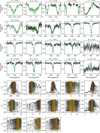 |
Fig. 2 KIWI-GA fit of A13. Top: best-fitting FASTWIND model (solid green line) and 1σ uncertainties (shaded green region) plotted on top of the observed spectrum (black vertical bars representing uncertainties; rebinned for clarity). Bottom: fitness plots for each parameter where darker coloured points represent models of later generations. The solid red line is the best-fit value, and darker and lighter yellow shaded regions represent 1- and 2σ uncertainty regions, respectively. |
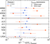 |
Fig. 3 Photospheric abundance determinations of C+N+O (blue) and Si (red) for each star as a fraction of solar compared to the adopted host galaxy metallicity, Z, from Table 2. Data points indicate whether the host galaxy metallicity Z was determined from nebular emission (circles) or through spectroscopic analysis of supergiants (squares). The vertical dotted line represents equality between our abundance determination and the solar value scaled to the adopted metallicity of the host galaxy. The troublesome runs of A11 and B11 are highlighted in grey. |
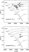 |
Fig. 4 Positions of the stars on the HRD overplotted on the evolutionary models of Szécsi et al. (2022, solid lines). The zero-age main sequence and isochrones of 1−6 Myr (spaced 1 Myr apart) are indicated with dashed lines. Top: Stars in IC 1613, NGC 3109, and WLM overplotted on the dwarfA model grid (0.1 Z⊙). Bottom: Stars in Sextans A and Leo P overplotted on the dwarfB model grid (0.04 Z⊙). |
4.5 Evolutionary status
In order to gauge the evolutionary status of the stars in this sample, we compare them to the Bonn Optimized Stellar Tracks (BoOST; Szécsi et al. 2022). Figure 4 shows the position of the stars on the Hertzsprung-Russell diagram (HRD). For the stars in IC 1613, WLM, and NGC 3109, we overplot stellar models from the dwarfA grid (0.1 Z⊙) and for those in the lower Z galaxies of Sextans A and Leo P, we overplot models from the dwarfB grid (0.04 Z⊙). Also shown are isochrones in steps of 1 Myr. We estimate evolutionary parameters by locating the position of each star in the interpolated grids within the uncertainties of L and Teff, the results of which are shown in Table 11.
All stars appear on the main sequence. In general, we see that, according to this set of single-star evolutionary models, the stars in Leo P and Sextans A are more evolved with an age >5 Myr, as found by Telford et al. (2021), while the other stars are ∼4 Myr in age, with A13 being an exception as it is quite young; around 2.5 Myr old. For 62024, B2, B11, A15, A11, and N34, we see a reasonable agreement between the current evolutionary mass, Mevol and the spectroscopic mass, Mspec, determined by the KIWI-GA fits. However, there are large discrepancies between these quantities for the other stars. This is no surprise given the well-established ‘mass discrepancy problem’ (Herrero et al. 1992; Weidner & Vink 2010). We do not comment further on this in this work.
The full main-sequence evolutionary timescale reported in the BoOST tracks for the stars in our sample range from ∼4−9 Myr. Given that the mass loss rates we derive are at most 10−7 M⊙ yr−1, they lose at most 0.1−1 M⊙ during this phase. Therefore, for stars up to initial masses of ∼50 M⊙ in sub-SMC metallicity galaxies, main-sequence mass loss, and hence main-sequence angular momentum loss, is of minor importance for evolution. If the initial rotation speed of the star is large, this favours an efficient rotation induced mixing of CNO-products throughout the star and opens the possibility of chemically homogeneous evolution (CHE) for initially very fast spinning sources (see e.g. Brott et al. 2011; Szécsi et al. 2022). The best candidate for CHE in our sample appears to be S3 in Sextans A for which we find 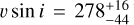 km s−1. Its HRD position, non-enhanced helium abundance, and constraints for its CNO-abundance pattern derived here (see Table 10), though with considerable uncertainties, do not suggest a CHE pathway.
Evolutionary parameters of our sample stars.
5 Discussion
In this section we discuss the implications of the results we have obtained. In Sect. 5.1 we quantify the dependence of Ṁ on L in this Z regime by examining the modified wind momentum (Dmom). In Sect. 5.2 we compare our obtained values of Dmom and Ṁ to the different theoretical predictions that exist for these quantities. We discuss implications of our findings in Sect. 5.3. In Sects. 5.4 and 5.5 we compare our results to previous analyses of SMC samples and samples of stars in lower Z galaxies. In Sect. 5.6 we discuss the values for v∞ that we obtain and compare them to an empirical relation, and in Sect. 5.7 we discuss potential consequences of the assumptions we have made in this work.
5.1 Fits of Dmom versus L
First, we provide a brief overview of the relevant parts of radiation-driven wind theory (Lucy & Solomon 1970; Castor et al. 1975, hereafter CAK; Abbott 1982), as we test the scaling relations predicted by the theory and compare our observations to the different predictions that exist. In CAK theory, the total line acceleration is expressed using a force-multiplier which is described by three parameters. One of these parameters is the ratio of the number of optically thick lines that contribute to the wind-driving force to the total number of lines: α. This is important as it quantifies how the mass loss rate, Ṁ, scales with L, the effective mass, Meff = M(1−ΓEdd), which is the mass of the star scaled by the Eddington parameter, and Z in the following relation (Puls et al. 2008):
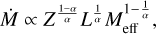 (5)
(5)
where the effect of a second parameter, the ionisation parameter δ, is neglected here as it is typically small (∼ 0.05−0.1; Abbott 1982). One quantity derived from CAK theory that is commonly used to examine the Ṁ(Z) dependence and to quantify α is the modified wind momentum, Dmom (Puls et al. 1996; Lamers & Cassinelli 1999). For a fixed Z, this quantity is given by
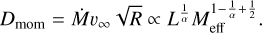 (6)
(6)
This is a useful relation because α is predicted to be ∼2/3 for O-type stars at ∼ Z⊙ (Puls et al. 2000), meaning the dependency on Meff, a notoriously uncertain quantity if determined spectroscopically (Sander et al. 2015), effectively drops out. In this case, one may fit the relation
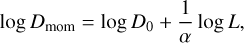 (7)
(7)
where log D0 is an offset term that captures the Z dependence.
However, recent analyses (discussed in Sect. 5.4) suggest α may actually decrease with Z. In this case, the Meff dependency becomes non-negligible, meaning it does not make sense to use Eq. (7), and the entire relation must be fit:
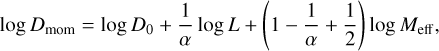 (8)
(8)
for a fixed Z and if α ≠ 2/3.
The top panel of Fig. 5 shows the position of the stars in our sample on the Dmom versus L diagram. Also shown is the empirical Dmom(L, Z) relation of Backs et al. (2024a). This was obtained from a sample of Milky Way, LMC, and SMC stars in the luminosity range log L/L⊙ = 5−6; we extrapolate this relation to lower Z and plot Dmom(L) at Z = 0.14 and 0.06 Z⊙.
Present in the top panel of the figure is the fit to Eq. (7). To account for the Z dependence, we chose to fit only the stars in IC 1613, WLM, and NGC 3109 and assume that these are of the same average Z ∼ 0.14 Z⊙. This is a reasonable approximation to make because the adopted metallicities of these galaxies are similar. We excluded A11 and B11 (squares with red borders) due to the issues faced in the fitting procedure as well as 64066, for which only an upper limit for Ṁ was determined. This means that a total of six stars are considered in the fit (the circles in the figure). To account for the uncertainties on both L and Dmom, we performed the fit using orthogonal distance regression (ODR; Boggs & Rogers 1990). From the slope, we obtain α = 0.21 ± 0.04.
We present the fit of Eq. (8), which incorporates the Meff dependency, to the same 6 stars in the bottom panel of Fig. 5. As this is a two dimensional fit as a function of both L and Meff, the best-fit solution to this equation is a plane. The best-fit solution of each star is therefore represented as a black point in Fig. 5 which depicts, for a given star, the point on the best-fit plane at its (L, Meff) values projected onto the L axis. By incorporating Meff into this, we obtain a value for α of 0.18 ± 0.06. This is consistent with that obtained from the fit of Eq. (7) and both values are significantly lower than the canonical value of 2/3.
We also perform this analysis using Ṁ and find similar results. This can be seen in Appendix E. That α < 2/3 in this low Z regime means that care should be taken when analysing Dmom of metal-poor massive stars, as the Meff dependence becomes non-negligible. From its definition, a lower α means that less optically thick lines are contributing to the radiation force driving the wind, thus decreasing the overall radiation force and resulting in weaker winds, as expected in lower metallicity environments. Future theoretical work should explore how α (in the CAK formalism) is expected to scale with Z.
 |
Fig. 5 Top: fit of Eq. (7) based on the six points denoted with circles. Overplotted with dotted lines is the empirical relation of Dmom(L, Z) determined by Backs et al. (2024a). Bottom: projection of the two-dimensional fit to Dmom(L, Meff) (Eq. (8)) onto the luminosity axis, shown by black points (see text for further details). In both plots, the square points have been excluded from the fits, red borders indicate troublesome fits, the value for α determined from the fit is provided and the metallicity of both the tracks and the points are colour-coded. Uncertainty regions on the fit have been excluded for clarity. In the top panel they are large and span the entire vertical range of the panel. |
5.2 Comparing Dmom(L) at Z = 0.14 Z⊙ and Ṁ to theory
In this section we compare the values we have obtained for Dmom and Ṁ to three theoretical predictions: those of Vink et al. (2001), Björklund et al. (2021), and Krtička & Kubát (2018).
5.2.1 Modified wind momentum
Figure 6 shows how our fit of Eq. (7) compares to three sets of theoretical predictions of Dmom(L). To make this comparison, we extrapolated the results of Björklund et al. (2021) and Krtička & Kubát (2018) to metallicities below that of the SMC. The first thing to notice is that all prescriptions yield a shallower slope (i.e. a higher CAK α) at Z ∼ 0.14 Z⊙ than our empirical result. Of the three sets, the Björklund et al. (2021) models have the steepest slope (i.e. have the lowest CAK α). Also, all predictions match best at the high L end of stars studied here. The prescription of Björklund et al. (2021) is consistent with the values of the individual stars at high L, disregarding A11 and B11. It really only overpredicts for B2, A15, and S3 – the stars in the low L end of the sample. The same can be said for the predictions of Krtička & Kubát (2018); however, it is less consistent at low L. The Vink et al. (2001) prescription predicts mass loss rates that are typically a factor of ∼2−3 higher than those by the other two works (e.g. Vink 2022). The reasons for this are possibly connected to the use of the energy equation rather than the momentum equation in constraining the wind properties (see Müller & Vink 2008 and Muijres et al. 2012 for a discussion of this), and to the use of the Sobolev approximation in computing the state of the gas. These authors overpredict Dmom of all stars except 64066, whose upper limit is consistent with the prescription.
In conclusion, available theoretical works predict a shallower Dmom(L) relation causing discrepancies with empirical rates at L ≲ 105.2 L⊙. Works requiring knowledge on the metallicity dependence of stellar winds may therefore best rely on empirical prescriptions (e.g. those of Backs et al. 2024a). If one wants to rely on theory, the prediction of Björklund et al. (2021) best represents our findings. This is consistent with previous studies (e.g. Backs et al. 2024a; Rickard et al. 2022; Telford et al. 2024), which we discuss in Sect. 5.4.
5.2.2 Mass loss rates
For completeness, we compare our determinations of Ṁ to the same three theoretical predictions, which can be seen in Fig. 7. Again, the prediction of Björklund et al. (2021) is closest to the values we obtain, with a spread of ∼±1 dex around a ratio of unity. That of Krtička & Kubát (2018) slightly overpredicts Ṁ of our sample, while that of Vink et al. (2001) highly overpredicts the mass loss rates of most of the stars by more than a factor of ten. This finding is in line with the conclusion formulated at the end of the previous subsection.
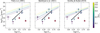 |
Fig. 6 Fit of Dmom(L) obtained in this work compared to three different theoretical predictions (dotted coloured lines). In each plot, the points and the fit shown are the same as those shown in the top panel of Fig. 5, as are the Z values of each theoretical track. The colour coding of the predictions is the same as in Fig. 5. Uncertainties in the fit span the entire vertical range of the panel. |
 |
Fig. 7 Ratio of the mass loss rate of the stars in the sample determined by the KIWI-GA fits (Ṁ) and the prediction of this value (Ṁpred). |
5.3 Implications of our results
In this section, we discuss the implications of our findings from Sects. 5.1 and 5.2. Our results indicate a fit of Dmom(L) at Z = 0.14 Z⊙ for six of the stars in our sample that is in fair agreement with an extrapolation of the empirical Dmom(L, Z) relation of Backs et al. (2024a) to this Z. Notably, this relationship, calibrated in the metallicity range from solar to 1/5th solar metallicity, predicts a steeper dependence on Z of Dmom at relatively low luminosity (L ≲ 105.2 L⊙) than what is predicted by theory (compare Figs. 5 and 6).
In this low L regime at Z ∼ 0.14 Z⊙, our findings suggest O stars experience minimal mass loss during their main sequence evolution. For a 40 M⊙ star, representative of the average luminosity of ∼105.4 L⊙ of our sample, a main sequence mass loss rate of ∼10−7−10−8 M⊙ yr−1 would remove only ∼0.05−0.5 M⊙ over the roughly 5 million years that this stage of evolution lasts (e.g. Brott et al. 2011; Szécsi et al. 2015). Consequently, the effect of main-sequence mass loss for mass stripping and angular momentum loss is much less significant for these stars compared to equally bright O-stars in higher Z regions.
Whether this also holds for their post-main sequence evolution remains to be investigated. If later on these sub-SMC metallicity massive stars experience a luminous blue variable (LBV) phase (see Herrero et al. 2010 for a discussion of LBV candidate V39 in IC 1613) during which mass is shedded efficiently, similar to what is hypothesised for Galactic stars (Smith 2014), the situation may be different, especially if the (unknown) mechanism for giant LBV eruptions is metallicity independent.
Additionally, we note that the ‘weak-wind’ problem has been observed in this low L regime (at L ≲ 105.2 L⊙; Vink 2022) at solar (Martins et al. 2005; Marcolino et al. 2009) and SMC metallicities (Martins et al. 2004). We find a steeper Dmom(L, Z) relation than what is predicted by theory, so this may be linked to it. Furthermore, it has also been shown that, in OB stars with these weak winds, material in the wind can be shocked to higher ionisation stages, meaning that the traditional wind signatures such as C IV or Si IV in the UV disappear, and instead the wind is detectable in the form of X-ray emission (e.g. Huenemoerder et al. 2012). This is a possible solution to the weak-wind problem, as a shocked wind scenario could result in lower Ṁ and/or v∞ inferred from the UV than the true values across all phases of the wind. Whether such X-ray emission is present in our sample stars is uncertain and would require dedicated observations to confirm. Given we see these traditional features form in the wind in all but one of our sample stars, this would suggest that this ionisation due to shocks has not taken place, at least not completely.
At the high luminosity end, at L ∼ 106 L⊙, the situation is different. Here, the empirical relation of Backs et al. (2024a) and the theoretical relations by Björklund et al. (2021) and Krtička & Kubát (2018) show a particularly weak metallicity dependence. Therefore, in this regime, massive stars in galaxies similar to those studied here may be capable of shedding (almost) as much mass as their counterparts in the Magellanic Clouds or even in the Milky Way. In fact, this further suggests that low Z stars at even higher L, in the regime of very massive stars, may be subject to the same upturn (or ‘kink’) in Ṁ as a function of ΓEdd as experienced by stars at higher Z (e.g. Bestenlehner et al. 2014). This occurs when the flux-weighted mean optical depth, τF, of the wind transitions from below to above 1 (Vink et al. 2011; Vink & Gråfener 2012). When the winds are optically thin (τF < 1),  until they grow denser and become optically thick (τF > 1) and this dependence sharply increases to
  To test this would require observations of more low Z stars with masses high enough to place them in this L regime.
We find that the stars in our sample only reach masses up to ∼30−50 M⊙ (Table 9), likely because they are found in regions of modest star-formation. If this is indicative of the general massive star population in these galaxies, mass loss is not as important in their evolution compared to similar L stars in higher Z regions. Vigorous star-formation, similar to the star-forming activity in the LMC (where the maximum stellar mass is ∼250−300 M⊙; e.g. Brands et al. 2022), is required to produce stars of at least ∼90 M⊙ or ∼106 L⊙ that would suffer strongly from mass loss (e.g. Köhler et al. 2015; Szécsi et al. 2015; Sabhahit et al. 2023).
5.4 Comparing Dmom(L, Z) to previous empirical studies
One of the first investigations of the Ṁ(Z) dependence was performed by Mokiem et al. (2007). In this study, they gathered samples of Milky Way, LMC, and SMC stars that had been studied with either FASTWIND or CMFGEN (Hillier & Miller 1998). They found, at log (L/L⊙) = 5.75, Ṁ ∝ Z0.83 ± 0.16 for smooth winds, or Ṁ ∝ Z0.72 ± 0.15 when clumping was accounted for. Furthermore, this derived dependence incorporated the terminal velocity scaling v∞ ∝ Z0.13 of Leitherer et al. (1992).
Backs et al. (2024a) analysed a sample of 13 SMC O-stars using Fastwind and KIWI-GA. These authors found that the predictions of Björklund et al. (2021) best match the mass loss rates of the stars in their sample. Further, using their results, along with the LMC samples of Brands et al. (2025) and Hawcroft et al. (2024a), and the Milky Way sample of Hawcroft et al. (2021), they derived an empirical fit for Dmom(L, Z) to which we compare our findings in previous sections. They found a stronger Z dependent L dependence on Dmom than what is suggested by theoretical predictions of this quantity. Our fit of six stars is relatively in line with their relation for Z = 0.14 Z⊙− the average metal content of the host galaxies of the stars considered in the fit.
Rickard et al. (2022) analysed the O-star population in the NGC 346 cluster in the SMC. Through analysis of Dmom, they found a steeper Z dependent L dependence of Ṁ than what is currently predicted; instead of a fixed scaling, say Ṁ ∝ Zx, they find x ∝ L−1.2, much steeper10 than the L dependence of L−0.32 predicted by Björklund et al. (2021).
A steep Z dependence was also found by Ramachandran et al. (2019). In this work, they fit Ṁ as a function of L for nine OB stars in the wing of the SMC. When considered along with the Ṁ(L) relation found by Ramachandran et al. (2018) for LMC stars, where Z = 0.5 Z⊙, they suggested a value for x ∼ 2. This is steeper than an exponent 0.69, as predicted by Vink et al. (2001), or 0.83, determined empirically by Mokiem et al. (2007).
On the other hand, Marcolino et al. (2022) found contrasting behaviour to the previous studies mentioned. They found, for their sample of Milky Way and SMC stars, that their fits of Dmom(L) for the two galaxies diverge towards higher L, as opposed to lower L as is seen in the aforementioned studies. They suggest this could be due to the large number of low L targets in their sample, where various factors can become important in this L regime, such as additional dependencies on α, like Teff for example, becoming non-negligible (Puls et al. 2000). In fact, when the low L targets are excluded from fits, they find good agreement with the empirical study of Mokiem et al. (2007).
Regarding what all of this suggests, apart from the study of Marcolino et al. (2022), all recent analyses of SMC samples have found a steeper metallicity dependence than what is currently predicted by theory. Our results are in line with this finding (see Fig. 5). To avoid uncertainties by comparing different studies that use different methods and assumptions, a full homogeneous analysis of Milky Way, LMC, SMC, and low Z stars would be extremely beneficial to gain further insight into the Z scaling of the winds of massive stars.
5.5 Comparing to other quantitative spectroscopic analyses of our sample stars
Here we discuss previous analyses that included our sample stars. In Appendix G11 we detail the methods used in each analysis in Table G.1 and tabulate our results along with those obtained in these analyses in Tables G.2 and G.3.
One of the first analyses of low Z (i.e. Z < ZSMC) environments was carried out by Tramper et al. (2014). In this study, the optical spectra of a sample of 10 stars from IC 1613, WLM, and NGC 3109 were analysed. They found a significant discrepancy between their results and theoretical predictions and concluded that these low Z stars produce winds that are stronger than predicted. However, these authors did not have access to the crucial resonance lines in the UV. These are much more sensitive to lower values of Ṁ compared to optical wind lines, notably Hα and, moreover, encode vital information about the acceleration behaviour of the wind outflow and the terminal velocity it can achieve. Therefore, without the UV spectrum in this low Z regime, mass loss rates ≲ 10−7 M⊙ yr−1 are uncertain, and v∞ and β become degenerate with Ṁ.
Tramper et al. (2014) made assumptions in order to navigate the problems regarding v∞ and β. For v∞, it was first scaled with the surface escape velocity, vesc where v∞ = 2.65 vesc (Lamers et al. 1995) and then scaled with Z as v∞ ∝ Z0.13. Garcia et al. (2014) found a large scatter around the canonical relation of v∞/vesc = 2.65, meaning this scaling may not hold in general, and recent results have found somewhat higher exponents in the v∞(Z) scaling of ∼0.2 (Hawcroft et al. 2021; Vink & Sander 2021). As for β, a value of 0.95 was adopted – a value predicted for O5 supergiants (Muijres et al. 2012) – but this could be an uncertain assumption, as, in the case of a rapid rotator, for example, it may depend on factors such as the angle of inclination at which the star is being observed (Herrero et al. 2012).
We demonstrate the problems of obtaining Ṁ from mere optical diagnostics in Fig. 8 where we show updated Dmom and L determinations from our optical+UV analysis compared to the optical only analysis of Tramper et al. (2014) for the stars in both of our samples. By including the UV spectra, we obtain lower Dmom values for all stars and, excluding the troublesome fits of A11 and B11, we find values for Dmom that are more in line with the empirical relation of Backs et al. (2024a). We also find different values for L for some stars, most notably N20. This is because the wind lines in the UV, and of course the other lines in this wavelength range, are sensitive to Teff, which impacts the luminosity determination. This highlights the necessity to include both the optical and UV spectra in the analysis of low Z massive stars.
Bouret et al. (2015) also highlight the importance of including the UV spectra in such analyses. They analysed the optical and UV spectra of A13, A11, and B11 and also found lower values for Ṁ than Tramper et al. (2014) (see Table G.3 for the values obtained in each study). For A13, we found a value for Ṁ consistent with theirs; however, we found lower values for A11 and B11. Regarding these latter two stars, Bouret et al. (2015) speculate that, for such weak winds, porosity and vorosity effects on wind structure and the presence of hot gas may severely bias the estimated mass loss rate. We revisit this in Sect. 5.7.1.
Interestingly, both Bouret et al. (2015) and Garcia et al. (2014) found evidence that the Fe abundance of the stars they studied may be higher than the typically adopted literature values for their host galaxies (IC 1613 for both authors, and WLM for Bouret et al. 2015) and are instead closer to an SMC-like abundance of 0.2 Z⊙. Bouret et al. (2015) found that models with Fe/Fe⊙ of both 0.14 and 0.20 were compatible with the Fe lines in the observed spectra, although there was some degeneracy with the micro-turbulent velocity, ξ. However, they argued that a value of 0.2 Z⊙ is a more realistic metallicity value for both galaxies. For the IC 1613 stars, their measured value of 0.2 Fe⊙ is consistent with iron abundances of late type stars (Tautvaišienė et al. 2007) and with the star formation history of the galaxy (Skillman et al. 2003). Garcia et al. (2014) concur with this, as they find that model spectra with Z = 0.2 Z⊙ were required for their analysis and that the spectra of the stars in their sample closely resemble stars in the SMC with the same spectral type. We return to the metallicity of IC 1613 in Sect. 5.7.2.
To conclude this section, we show that the UV spectra are necessary when analysing the wind properties of low Z massive stars, as previously shown by Bouret et al. (2015) and Garcia et al. (2014).
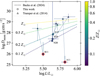 |
Fig. 8 Comparing the values obtained for Dmom in this work (circles) to those obtained by Tramper et al. (2014) (triangles). Solid lines join the (L, Dmom) pairs obtained for the same star but in the two different studies. |
 |
Fig. 9 Terminal velocities overplotted on the empirical relation of Hawcroft et al. (2024b). The black dashed line represents an ODR fit through the circle points. As B2 and A15 have the same Teff, that of the former has been offset by −250 K for clarity. For similar reasons, that of B11 has been offset by +250 K. |
5.6 Terminal velocities
The determination of the terminal velocity, v∞, proved to be quite challenging for many of the stars in this sample. Because of the weak winds of these stars, many do not have saturated P Cygni profiles, with some barely showing any wind signatures. In these cases, both v∞ and β are hard to constrain. There are, however, stars with C IV λ1550 features that show a well defined P Cygni profile (A13, N20, N34), so the parameters obtained for these stars can be considered robust. Furthermore, for the very low metallicity stars, LP26 and S3, we find very low values of  and
and  km s−1, respectively, consistent with Telford et al. (2024).
We compare our findings to the empirical relation of Hawcroft et al. (2024b). They analysed the C IV λ1550 profiles of samples of Milky Way, LMC, and SMC stars. If the profile was saturated, v∞ was determined from the bluest edge of the P Cygni absorption trough, while the SEI method (Lamers et al. 1987) was employed if the profile was not saturated. As this relation was only determined from stars with metal contents as low as SMC metallicity, we extrapolate it here.
Figure 9 shows v∞ obtained for the stars studied in this work overplotted on the relation of Hawcroft et al. (2024b) at Milky Way, LMC, and SMC metallicity, and extrapolated to lower metallicities of 0.14 Z⊙ and 0.06 Z⊙. We perform an ODR fit through our data, for which we limit ourselves to the same six points as used to fit Dmom in Fig. 6; that is, we excluded 64066, S3 and LP26, and those for which the spectral fits were of poor quality (B11 and A11). We find that the fit is consistent with the empirical relation at 0.14 Z⊙. However, there is a lot of scatter. The uncertainty region has been excluded for clarity, but it covers all other empirical tracks. This is a small sample whose v∞ values were determined from low resolution and low S/N spectra. Care must therefore be taken with this fit; a larger sample of higher resolution spectra is needed to infer more about this. Furthermore, as discussed in Sect. 5.3, if X-rays are shocking material in the winds of these stars, the values for v∞ may potentially be underestimated here, especially in S3 and LP26. Finally, we remark that the terminal velocities of the three fitted sources in IC 1613 (A13, B2, and 62024) are not remarkably high relative to the other three fitted sources.
 |
Fig. 10 Comparison between the best-fitting FASTWIND models determined by KIWI-GA where optically thin clumping was assumed (green), a FASTWIND model with the same stellar and wind parameters but with a smooth wind (i.e. fcl = 1; blue dashed line), and a smooth FASTWIND model (again) with the same stellar parameters as the KIWI-GA fit but with a mass loss rate scaled by a factor of |

5.7 Impact of our assumptions
As in all modelling, for practical purposes, we have made a number of simplifying assumptions to achieve the goals of this paper. In this section we examine the potential consequences of making such assumptions which will inform future work once larger samples become available. First, in Sect. 5.7.1, we discuss the assumptions we have made regarding the wind structure, particularly in the context of A11 and B11. Then, in Sect. 5.7.2, we examine our assumption that the metal content of the stars in our sample are equal to those of their host galaxy, given in Table 2.
5.7.1 Wind structure
Here, we first comment on the robustness of the values we obtain for the clumping factors in the optically thin clumping formalism. We then discuss possible effects of optically thick clumping, and conclude this section with a discussion of A11 and B11 in this context.
Optically thin clumping. As mentioned in Sect. 4.2, many of the values we obtain for fcl are largely unconstrained as they have large uncertainties – some spanning the entire parameter space. This raises the question whether these values hold physical significance or are a result of overfitting. We tested this on a number of stars in the sample: A13, N20, and A15, with reasonably well constrained posteriors of fcl, and N34, whose values are essentially unconstrained.
We demonstrate this in Fig. 10. The green fit represents the best-fitting FASTWIND models and 1σ uncertainties determined by KIWI-GA with optically thin clumping implemented. To see if the UV resonance lines are clumping sensitive in this Z regime, we first calculated FASTWIND models with identical parameters as the best fitting stellar and wind parameters determined by KIWI-GA but with a smooth wind, shown as the dashed blue lines in the figure. We find that these features are indeed sensitive to variations in fcl, provided they are formed in the wind, as wind features become photospheric (C IV λ1550 for A13 and A15, and Si IV λ1400 for N20 and N34). For A13, the reason why the C IV λ1550 profile becomes photospheric in the model with a smooth wind is because C V is the dominant ionisation stage of carbon in the wind here, which results from its high Teff of ∼45 kK, and therefore no C IV is seen in the wind. This is because the recombination rate increases quadratically with density, while the ionisation rate increases only linearly. Therefore, in the model with a clumped wind, C IV is the dominant ionisation stage due to the increased recombination from C V in the overdense regions, resulting in a well-developed P Cygni profile.
To compensate for the lack of clumping, we then calculated smooth FASTWIND models, again with the same best-fitting stellar parameters determined by KIWI-GA, but with a larger mass loss rate scaled by  ; where fcl,GA is the best-fitting clumping factor determined by KIWI-GA. For A13, we see that, while C IV λ1550 is formed in the wind at this increased Ṁ, there is also a wind signature in Hα as the line core is filled in, which is not observed in the spectrum. For N20, this test model reproduces the Si IV feature reasonably well but saturates the C IV profile, which is not observed in this star. For N34, the test model reproduces the C IV profile, but is unable to reproduce the absorption observed in the blue feature of the Si IV doublet. This minimal change in the shape of the C IV profile can be expected in these two stars as it is saturated in both models, meaning it is less affected by clumping (e.g. Bouret et al. 2005). Finally, for A15, we can see that clumping is required to reproduce the blue absorption in the C IV λ1550 line. These discrepancies suggest that wind inhomogeneities should be accounted for in stars in this Z regime.
We conclude that, provided they are formed in the wind, the UV resonance lines in the spectra of stars in this Z regime are sensitive to variations in fcl in the optically thin clumping formalism implemented in FASTWIND. As such, these features can provide somewhat meaningful constraints on the clumping factor. This suggests that our obtained values of fcl for our sample stars with non-saturated wind signatures in their spectra are not entirely a result of overfitting.
Optically thick clumping. In Fig. 11, we present test calculations assessing the possible effects of the assumption of optically thin clumping as well as other assumptions we made on two stars: A13 and A15. These stars are the most and least luminous, respectively, considered in the Dmom(L) fits in previous sections.
We tested the possibility that the wind contains an ensemble of clumps that may range from being optically thin to optically thick (see Sect. 3.1). For a detailed explanation of this so-called macro clumping assumption and the way in which it is implemented in FASTWIND, we refer to Sundqvist et al. (2018); Brands et al. (2022).
In the figure, we compare our adopted results, shown in blue, to a KIWI-GA fit adopting different assumptions, shown in red. For A13, optically thick clumping is assumed in this additional KIWI-GA run and vwindturb is left as a free parameter, while for A15, only optically thick clumping is assumed. We also show the effect that this has on the determination of the wind parameters Ṁ, v∞, and fcl in panels on the right side of the figure. We decide to leave vwindturb free for A13 only in this test because it is clear, from the mismatch of our best-fit model and the blue edge of the C IV λ1550 profile, that our assumed value of 0.14 v∞ is too large. Such a conclusion cannot be drawn from the fit of A15, as its wind features are not as prominent.
This optically thick clumping formalism in FASTWIND allows for the inter-clump density contrast, fic, to be left as a free parameter and also accounts for velocity porosity in the wind. Velocity porosity is a measure of the velocity dispersion within the clumps and is described by a factor fvel (see, e.g. Sundqvist & Puls 2018; Brands et al. 2022), which we make a free parameter in this exercise. To allow for a more thorough exploration of the parameter space, we fix v sin i in each run to the value determined from the original fit where optically thin clumping was assumed. We show the results obtained from the fits in Table 12.
For A13 (top row of Fig. 11), we find that the assumption of optically thick clumping and leaving vwindturb free does not significantly affect the determinations of Ṁ, v∞, and fcl, as they are equal within 1σ uncertainties. We note that the fit to the C IV λ1550 profile is better if we assume optically thick clumping and fit vwindturb. However, this is probably more affected by the latter. If vwindturb is lower than what we assume, the blue edge of the P Cygni profile will be steeper, as there is less excess velocity at v∞ in the wind. Furthermore, the smaller vwindturb allows for the best-fitting FASTWIND model to reproduce the blueshifted doublet absorption feature at ∼1540 Å. In this new fit, a lower value of  is found that is closer to the value of 0.8 obtained by Garcia et al. (2014) and Bouret et al. (2015), though still equal within uncertainties to the higher value obtained in the original, optically thin fit. Other than this, we find no significant differences between the two assumptions for the rest of the line profiles.
Here we find that  v∞ for A13 – significantly lower than the value of 0.14 v∞ that we assume, and the value of (0.14 ± 0.06) v∞ determined from the LMC sample of Brands et al. (2022). This could suggest that lower Z stars exhibit lower turbulence in their winds, but this needs to be further investigated. This must be explored with high-resolution and high S/N spectra of more stars that exhibit P Cygni profiles.
For the case of A15 (bottom row), if the clumps are allowed to become optically thick, we find an Ṁ that is a factor of approximately six higher than that obtained in the optically thin case while also finding a value for v∞ that is equal within uncertainties to that obtained when optically thin clumping was assumed. As Ṁ can be affected, this test shows that the assumption of optically thick clumping may influence the slope and offset of the Dmom(L) relation.
That being said, we do find that a smooth wind cannot be ruled out in the optically thick KIWI-GA fit of A15, as  here. This value is significantly lower than that obtained from the fit under the assumption of optically thin clumping, where
  . Such a change in fcl can change the shape of the C IV λ1550 profile, and consequently, Ṁ. This introduces a degeneracy between Ṁ and fcl. The modest S/N of the data, combined with the limited diagnostic features present in the spectra of these low Z targets, makes it difficult to break this degeneracy at the present moment. Furthermore, due to the large uncertainties on the data for this star, the fits from both runs are consistent within uncertainties. Future work should investigate the effects of optically thick clumping in low Z stars and their potential impact on the Dmom(L) relation.
B11 and A11. As mentioned in Sect. 4.3, our KIWI-GA fits to these stars were not satisfactory. Therefore we did not include them in the Dmom(L) fits in Sect. 5.1. To test whether this was an issue of an insufficiently large parameter space, we show for both stars, in Fig. 12, the best-fitting FASTWIND models of the common features between the two stars that are poorly fit, C III λ1176, Si IV λ1400, and Hα, and compare them to the overall best-fitting FASTWIND model determined by KIWI-GA. For both stars, the best-fitting models for each line provide improved fits compared to the overall best-fitting model. The core of the C III λ1176 profile is desaturated for both stars and the red wing is better reproduced for A11. The blue absorption of both features of the Si IV doublet is captured by the best-fitting model of this line complex for both stars (not so much for the blue component of A11), while the red emission is still not present in these models. The Hα profile of the best-fitting model of this line is better fit for both stars than the best-fitting overall model. For these stars, no unique set of fitting parameters can simultaneously provide a satisfactory fit for all lines in the spectra of these stars, while models with different combinations of parameters can provide good fits individually. This suggests that there may exist a more optimal solution using some combination of parameters from outside the parameter space. However, this could also mean that there are some other effects at play in these stars that are not accounted for by our assumptions made in this work, which we explore next.
These stars were also analysed by Bouret et al. (2015) who similarly reported low Ṁ values. They suggest that their values may be underestimated due to a more complex wind structure than simply optically thin clumping, with spatial- and velocity-porosity effects possibly becoming important.
They investigate this hypothesis by computing a model for A11 with a wind structure that mimics a wind with hot gas that does not contribute to the UV spectrum. Focusing on the C III λ1176 and Si IV λ1400 lines only, they found that this new model better reproduced the observed features by desaturating the centre of the C III λ1176 line and exhibiting red emission and blueshifted absorption in the Si IV λ1400 line.
We also find that our best-fitting FASTWIND model cannot reproduce these features in these lines for B11 and A11 (whose fits are shown in Figs. H.4 and H.6, respectively, and as shown above). Therefore, to test the statement of Bouret et al. (2015), specifically regarding the impact of porosity in the winds, we performed KIWI-GA fits for these stars assuming optically thick clumping, where this effect is accounted for. We found a similar unsatisfactory fit for A11, so we only discuss B11 here. Figure 13 shows, for B11, the C III λ1176, Si IV λ1400, and C IV λ1550 lines and the best-fitting FASTWIND models determined by KIWI-GA where optically thin (blue) and optically thick (red) clumping has been assumed. We find similar results to Bouret et al. (2015), namely that, when optically thick clumping is assumed, the centre of the C III line desaturates (albeit at the expense of excess blue absorption), the blue absorption and red emission in the Si IV line is reproduced within uncertainty, and that Ṁ increases by a factor of ∼10.
This shows that the assumption of optically thick clumping in FASTWIND can help reproduce features in observed line profiles that optically thin clumping cannot account for, suggesting that these effects may indeed become important in the winds of these stars as hypothesized by Bouret et al. (2015). Furthermore, because a unique solution was found here using stellar and wind parameters from the original parameter space explored (albeit with the introduction of new free parameters like porosity), this suggests that the parameter space explored in the optically thin runs are sufficient and the original troublesome fits are more likely due to effects not accounted for by our original assumptions. However, as noted above, the optically thick clumping formalism in FASTWIND introduces a number of extra free parameters that are difficult to constrain with data of this quality. Therefore, care should be taken when interpreting this.
Best-fit parameters for A13 and A15 where optically thick clumping has been assumed.
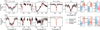 |
Fig. 11 Comparing the optically thin formalism used in this work (blue) to the optically thick formalism (red) for A13 in IC 1613 (for which vwindturb is also a free parameter; top) and A15 in WLM (bottom). Also shown in the three rightmost plots are the best-fit (solid line), 1σ (dark shaded region), and 2σ (light shaded region) uncertainties obtained for Ṁ, v∞, and fcl for both runs. |
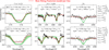 |
Fig. 12 Best-fitting FASTWIND models per line determined by KIWI-GA (red) compared to the overall best-fitting FASTWIND model and 1σ uncertainties (green) in the optically thin formalism. The top and bottom rows are B11 and A11, respectively. On each axis, the main parameters of the best-fitting model of the line shown on the axis are given. For comparison, we give the parameters of the overall best-fitting model determined by KIWI-GA on the side of the figure. |
 |
Fig. 13 KIWI-GA fits of B11 where optically thin (blue) and thick (red) clumping has been assumed. As in Fig. 11, we show the best-fitting values and uncertainties for Ṁ, v∞, and fcl obtained in each run. |
5.7.2 Adopted metal contents
As mentioned in Sect. 2.1 and discussed in Sect. 5.5, it has been suggested that IC 1613 and WLM may have higher metal contents than have been assumed in this work, and are probably closer to an SMC-like value (Garcia et al. 2014; Bouret et al. 2015). This would therefore affect the Dmom(L) fits presented in previous sections as 0.2 Z⊙ is considerably different to the other lower metal contents. Here, we examine this for IC 1613 only, as indications for a higher metallicity appear somewhat more substantial for this dwarf irregular.
We investigated the potential consequences of our assumed metallicity of 0.16 Z⊙ for this galaxy by performing KIWI-GA fits for these stars with metallicities of 0.2 Z⊙ instead, and then fitting Dmom(L) both for these stars alone and for the stars in the lower Z galaxies. In Appendix F, we present figures where for the same source, fits for different Z are compared; we also provide comments on these new fits. The fit of B11 was, again, troublesome as it had similar issues with that of the lower Z case, while the rest of the fits were satisfactory. We therefore only fit Dmom(L) for B2, 62024, and A13 in this case, and perform a separate fit for A15, N34, and N20, assuming an average Z of ∼0.13 Z⊙. The resulting Dmom(L) fits are shown in Fig. 14 where, unless otherwise stated in the legend, colours and symbols have the same meanings as in Fig. 5. We also show the uncertainty region as it is clearer than for the case where all six stars were fitted together.
Both fits produce a different slope and therefore a different α, the two values of which are quoted in the bottom right of the figure. The higher Z IC 1613 sample resulted in a higher α than that of the lower Z sample, which is to be expected from CAK theory. The higher Z fit is now in line with the empirical relation of Backs et al. (2024a) at 0.2 Z⊙, albeit rather uncertain as it is consistent with the LMC line but also the 0.13 Z⊙ line within 1σ uncertainties. The fit of the lower Z sample is positioned lower than the SMC line and is consistent with 0.13 Z⊙ line. The slopes of both fits are in good agreement with the empirical relation of Backs et al. (2024a) and the higher positioning of the IC 1613 stars is, at face value, in line with the suggestion that perhaps the metallicity of this galaxy is more SMC-like.
However, the sample size (three stars per fit) is very small. Therefore, at the present moment, the trade-off that has to be made is one between further reducing an already small sample size or having a larger sample (of six stars) and assuming the same average Z. Future work incorporating larger samples will be able to better account for different metallicities.
 |
Fig. 14 Separate fits of Dmom(L) for the stars in WLM and NGC 3109 (circles) and IC 1613 (diamonds). The points representing the stars of IC 1613 are from KIWI-GA runs where Z = 0.2 Z⊙ was assumed. Grey shaded regions represent 1σ uncertainties on the lines of best-fit. Square points have not been included in the fit and red borders indicate troublesome runs. The colour scheme is the same as that of Fig. 5. |
6 Summary and conclusions
In this work, we have analysed the combined optical and UV spectra of a sample of 11 O-stars in nearby dwarf galaxies with Z < 0.2 Z⊙. These eleven stars in the irregular dwarf galaxies IC 1613, WLM, NGC 3109, Sextans A, and Leo P constitute the full sample for which both spectral ranges are currently available in the literature. We used KIWI-GA and FASTWIND to determine the stellar and wind parameters for each star. Given the large distances to these galaxies and the quality of the spectra (with S/N ∼2−8 in the UV and ∼10−60 in the optical at a modest spectral resolution), we opted to assume that clumps in the outflows are optically thin. Our main findings are summarised as follows:
We corroborate the important finding by Garcia et al. (2014) and Bouret et al. (2015) that constraining mass loss rates of O-type stars in galaxies of metallicities below that of the SMC (with Z = 0.2 Z⊙) requires ultraviolet spectra of resonance line ions such as C IV λ1550. If only optical spectra are available, with Hα as the primary wind diagnostic, mass loss rates may be overestimated by as much as an order of magnitude;
We compared our fit of the modified wind momentum Dmom (a measure of wind strength that most easily allows for a comparison of stars with different Z and for a confrontation with theory) with the most sophisticated empirical relation currently available for Dmom(L, Z), which so far is established for the metallicity range Z = 0.2−1 Z⊙ (see Backs et al. 2024a). Using the six stars for which the wind strength is most reliable, we find that at (an average) 0.14 Z⊙, their modified wind momenta are in line with this empirical relation (Fig. 5). This supports the conclusion discussed and reviewed in Backs et al. (2024a) that at a lower L, mass loss shows a steeper Z dependence than at a higher L;
The slope of Dmom(L) is a measure of the line-force parameter α in CAK theory. For the six stars with Z ∼ 0.14 Z⊙ mentioned above, in IC 1613, WLM, and NGC 3109, we find α = 0.21 ± 0.04 when ignoring mass effects. If a mass dependence is considered in CAK theory, α = 0.18 ± 0.06. The steepness of the slope, mentioned in the previous finding, linked to the low α values at Z ∼ 0.14 Z⊙ mentioned here is not reproduced by hydrodynamical simulations of wind driving. These simulations predict a shallower Dmom(L) dependence at the metallicity of our sample stars;
Empirically, in the metallicity range Z = 0.2−1.0 Z⊙, it is found that the terminal flow velocity v∞ is less at a lower metallicity (Hawcroft et al. 2024b). The sample is currently too small to make meaningful statements regarding a v∞(Z) behaviour at lower metallicity.
Local Group irregular dwarf galaxies with metallicities below that of the SMC (at Z = 0.2 Z⊙) are probes of the environmental conditions in massive galaxies before the peak of cosmic star formation at redshift 2–3 (Madau & Dickinson 2014; Stanton et al. 2024). Establishing the properties of populations of massive stars in these nearby galaxies is therefore key for calibrating current theories of stellar atmospheres and evolution of these objects, which provide predictions of statistical properties of the end-of-life products of massive stars, including supernova types and black hole masses. For both of these evolution outcomes, an understanding of mass loss properties of O-type stars is crucial. To this end, future analyses using stellar atmosphere codes that can be used to infer the iron abundances of these metal-poor stars, such as PoWR, as was used by Telford et al. (2024), would be useful. Our study represents the most comprehensive and complete study of these properties at Z < ZSMC to date and reveals (and strengthens earlier indications) that theoretical expectations and empirical findings do not fully match toward low L. Larger samples of such objects are needed. The first steps to enlarge the sample of UV spectra are underway with ongoing low- and moderate-resolution HST observations (Program ID: 17491, PI: Telford), and a giant leap forward in securing optical spectra can be expected once the second-generation multi-object spectrograph MOSAIC is mounted on the Extremely Large Telescope.
Data availability
Appendix G, which contains a comparison with literature values of the sample stars, and Appendix H, presenting our KIWI-GA fits to our sample stars, are available online at Zenodo (https://zenodo.org/records/15078070). Other data may be made available upon request to the lead author.
Acknowledgements
We thank the anonymous referee for the insightful comments that have helped to improve the quality of this manuscript. We thank SURF (https://www.surf.nl/) for the support in using the Dutch National supercomputer, Snellius. OGT acknowledges support from a Carnegie-Princeton Fellowship, through Princeton University and the Carnegie Observatories. FB acknowledges the support of the European Research Council (ERC) Horizon Europe grant under grant agreement number 101044048. F. Tramper and M. Garcia gratefully acknowledge support by grant PID2022-137779OB-C41, funded by the Spanish Ministry of Science, Innovation and Universities/State Agency of Research MICIU/AEI/10.13039/501100011033, and M. Garcia further acknowledges grant PID2022-140483NB-C22. J. Gomez-Mantecon acknowledgements CSIC funding by the JAE Intro program JAEINT_24_01658. Based on observations with the NASA/ESA Hubble Space Telescope obtained at the Space Telescope Science Institute, which is operated by the Association of Universities for Research in Astronomy, Incorporated, under NASA contract NAS5-26555. Support for Program number GO-15967 was provided through a grant from the STScI under NASA contract NAS5-26555. This work was supported by a NASA Keck PI Data Award, administered by the NASA Exoplanet Science Institute. Data presented herein were obtained at the W. M. Keck Observatory from telescope time allocated to the National Aeronautics and Space Administration through the agency’s scientific partnership with the California Institute of Technology and the University of California. The Observatory was made possible by the generous financial support of the W. M. Keck Foundation.
Appendix A SIMBAD-resolvable names
In this section we provide, in Table A.1, identifiers of the sample stars that allows one to easily find them on SIMBAD.12
SIMBAD-resolvable target names of the sample stars.
Appendix B Abundances as mass fractions
Here we provide the best-fitting abundances for our sample stars determined by KIWI-GA in the form of mass fractions in Table B.1.
Appendix C Diagnostic spectral line list
In this section we provide, in Table C.1, a list of the spectral lines used in this work to determine the stellar parameters of our sample stars. In some stars, C III λ4070, C IV λ5801, and N IV λ6380 were modelled, but these were not present in the observed spectra and best-fitting FASTWIND models, and had no influence on parameter determination, so these profiles are not shown in the plots that show the best fits.
Spectral lines examined in this work. Within each line complex, we show the lines of each ion considered.
Appendix D Comments on individual targets 64066
64066 is the only star without a G160M spectrum, meaning the C IV λ1550 line could not be modelled. Due to our modelling approach, in that we chose not to include the N V λ1240 line due to its sensitivity to X-rays, no strong wind signatures were present in the UV, so upper limits for Ṁ were determined from optical recombination lines.
As there were no strong wind signatures present in the available UV resonance lines, we had to assume values for v∞ and β. For v∞, which is constrained by the absorption troughs of P Cygni profiles, we took the bluemost edge of the N V λ1240 line as an estimate, which gave 2000 km s−1, and adopt conservative uncertainty estimates of ± 200 km s−1. For β, which is constrained from the shape of a P Cygni profile, we assumed a value of 0.95. Overall, the fit is good as all lines are reproduced within uncertainties (Fig. H.1).
The only time 64066 was analysed before was in Herrero et al. (2012). In this study, they only determine a lower limit on the effective temperature of 49 kK, and log g = 3.8 from the optical spectrum alone. We find significantly lower Teff and log g values than Garcia & Herrero (2013) of  Kk and
  respectively. Furthermore, they used a grid search approach, where the models of the grid had a fixed ξ = 10 km s−1. From our combined optical and UV analysis, we find a factor of two higher value of this quantity.
A13
A13 has the highest quality spectrum of the entire sample in that it has a C IV λ1550 feature in the form of a developed P Cygni profile, a NIV λ1718 feature showing a wind signature, and strong He II lines in the optical. We therefore used this star to converge on our modelling approach.
Overall, the fit is good (Fig. 2). As for the UV fit, one of the components of the C III λ1176 complex at ∼1175.75 Å is not reproduced and the bottom of the absorption trough C IV λ1550 is not reproduced by our best-fit models (however, this is due to fixing vwindturb; see Sect. 5.7 for a discussion of this). As for the optical spectrum, the He II λ4686 of our best-fit model is too deep. Given the rest of the He lines are well reproduced, this line is probably sensitive to some other assumptions we made, perhaps where the onset of clumping begins.
Our best-fit parameters are generally in line with those obtained by Bouret et al. (2015), although we find it to be slightly hotter. Our v∞ values are consistent with both theirs and that determined by Garcia et al. (2014).
62024
The optical spectrum of this star was previously analysed by Herrero et al. (2012). Through the analysis of the He II λ4686 profile that was in the form of a P Cygni profile in their low resolution VIMOS spectrum, they found a high value of β = 2.0 for this star, as anything lower failed to reproduce this profile. From this, they conclude that 62024 may be a fast rotator seen pole on due to different wind conditions between the equator and the pole that are captured in this high β value.
We also find a high β value, consistent with a value of 2. We also find a relatively high v sin i = (160 ± 55) km s−1. However, we have neglected macroturbulent broadening effects, which may become significant in stars with a sufficiently high ΓEdd. We therefore cannot disprove this hypothesis that it is a fast rotator.
Our values for β and v∞ are also in line with those determined by Garcia et al. (2014) within uncertainties. The fit is satisfactory (Fig. H.2).
B2
The fit to B2 is satisfactory (Fig. H.3). Only the N IV λ1718 feature is not properly reproduced by our best-fit. Our β and v∞ determinations are consistent with the values determined by Garcia et al. (2014, their 65426) within uncertainties, as are our Teff and log g values with Garcia & Herrero (2013).
B11
We faced issues fitting this star which have been subject to discussion in Sect. 4.3, meaning it was excluded from fitting. The fit to the optical spectrum is satisfactory apart from discrepancies with the Hα feature. Potentially, macroclumping effects, such as spatial and velocity porosity, may be at play in the winds of this star, as we discuss in Sect. 5.7.1. The fit to this star is shown in Fig. H.4
A15
This fit is satisfactory overall (Fig. H.5). All lines in the UV and optical spectrum are well reproduced by our best-fit model. The only exception is the C IV λ1169 line, the profile of which is slightly too deep in the best-fit model compared to the data. We find stellar and wind parameters generally consistent with those found by Telford et al. (2024) for this star, only we find a lower log g.
A11
We faced similar problems as B11 in the fit for A11 (Fig. H.6). This star could potentially be a binary due to an abnormally large luminosity for its spectral type, as speculated by Bouret et al. (2015).
N20
The fit to this star is for the most part satisfactory (Fig. H.7). The fits to the wind features – the C IV λ1169 + C III λ1176 blend, Si IV λ1400, and C IV λ1550 – are good, as are those of the hydrogen Balmer and He I lines. Also sufficiently fit within uncertainties are the He II lines, apart from the one at 4686 Å. This is not immediately evident, since the spectra have been rebinned for clarity.
The He II λ4686 is not matched by our best-fit model. Interestingly, this feature in the spectrum of Tramper et al. (2011) and Tramper et al. (2014) is filled in, while ours is in absorption. This anomaly cannot be explained. The ‘Programme ID’ in the .fits file containing the spectrum is the same as that given in Tramper et al. (2011) where the observation of this star was carried out. There could perhaps be a difference in data processing between our work and theirs that is not immediately evident. We note that the PROCSOFT entry of the header of the .fits file says that the ‘xshoo/2.3.12dev1’ version of the ESO pipeline was used to reduce the spectrum contained in the .fits file used in this work, while Tramper et al. (2011) state the X-Shooter pipeline v1.2.2 was used to reduce their data.
Given the rest of the wind lines are sufficiently fit, this star is not excluded from the Dmom analysis.
N34
The fit for N34 is shown in Fig. H.8. Overall the fit is satisfactory, as all models reproduce the observed spectrum within uncertainties. What is notable are the large uncertainties on the parameters, especially the >1 dex uncertainty on Ṁ. That, and the large uncertainties on log g, which translate to uncertainties on R and therefore Dmom, which are evident in Fig. 5.
This large uncertainty on Ṁ is due to the low resolution and S/N of the G140L spectrum. Closer inspection of the fit revealed that only the Si IV λ1400 and C IV λ1550 lines favoured Ṁ = 10−7 M⊙ yr−1 with a large error margin, while all optical wind features as well as the He II λ1640 in the UV were insensitive for Ṁ < 10−6 M⊙ yr−1. Therefore, this combination of the many optical lines where only upper limits were determined and the two UV lines where a single Ṁ was slightly more favoured than this upper limit, resulted in a final determination with large uncertainties.
S3
Fig. H.9 shows the fit for S3. Given its large distance, its UV spectrum is especially noisy. It shows negligible wind features, meaning only upper limits for Ṁ can be obtained. This can be seen from the posterior of Ṁ in Fig. H.9. Nonetheless, the fit is satisfactory. We find that it is slightly hotter and has slightly higher log g than that determined by Telford et al. (2024), while the rest of the parameters are generally consistent.
LP26
LP 26 is the most distant and most metal-poor star in the sample. Similar to S3, only upper limits for Ṁ could be determined for this star. The fit, shown in Fig. H.10, is satisfactory; however, the terminal velocity could not be constrained. We obtain parameters consistent with those of Telford et al. (2024).
Appendix E Mass loss rates fits
Here we show a figure equivalent to Fig. 5 for Ṁ. We find low values of α consistent with that obtained from fitting Dmom, and consistent values depending on whether Meff is included in the fit or not. We also find a trend of Ṁ(L) that is steeper than that predicted by Björklund et al. (2021) at Z ∼ 0.14 Z⊙ at low L.
 |
Fig. E.1 Fits of Ṁ(L) (top) and Ṁ(L, Meff) (bottom) for the stars in the sample, where, as in Fig. 5, only stars with reliable Ṁ determinations are considered. Overplotted in the top panel are the theoretical predictions of Björklund et al. (2021). |
Appendix F Fits of IC 1613 stars at different Z
Here we present a comparison of the fits of the IC 1613 stars at the adopted metal content of the galaxy in this paper, 0.16 Z⊙, and KIWI-GA fits of these stars at 0.2 Z⊙. We show the best-fit parameters and uncertainties in Table F.1 and compare the best-fitting spectra in Fig. F.1.
We would also like to note some of the differences between the KIWI-GA fits at higher Z for these stars and those at lower Z so as to explain the position of the former on the Dmom(L) versus L diagram (Fig. 14). All stars appear higher on this diagram at higher Z. As for A13 and 62024, Dmom and log L are equal within uncertainties between the two KIWI-GA runs, as are the rest of the parameters. Therefore the same optimal local minima were found for each run.
The case of B2 is different. While L has remained the same between runs, Dmom is substantially higher in the higher Z run, which is something one would not expect. This can be explained by the carbon abundances, ϵC, obtained by the two KIWI-GA fits. The lower Z run found  , while the higher Z run found
  . To compensate for this decrease in ϵC, a larger Ṁ was consequently preferred. Due to the modest S/N of the spectra of the stars in this sample (∼ 5−10 in the UV) and degeneracies among the free parameters, these permutations of Ṁ and ϵC are seen as equally optimal by KIWI-GA and even the photospheric C lines cannot tightly constrain the C abundance.
Best-fit parameters of A13, 62024, and B2, from KIWI-GA runs with 0.2 Z⊙.
 |
Fig. F.1 Comparison of KIWI-GA fits of the three stars in IC 1613 considered in the fitting in Sect. 5.7.2 at 0.16 Z⊙ (blue) and 0.2 Z⊙ (red) of A13 (top), 62024 (middle), and B2 (bottom). Similar to Fig. 11, we show the best-fit values and uncertainties of Ṁ and v∞. |
References
- Abbott, D. C., 1982, ApJ, 259, 282 [Google Scholar]
- Asplund, M., Grevesse, N., & Sauval, A. J., 2005, in Astronomical Society of the Pacific Conference Series, 336, Cosmic Abundances as Records of Stellar Evolution and Nucleosynthesis, eds. I. Barnes, Thomas G. & F. N. Bash, 25 [Google Scholar]
- Backs, F., Brands, S. A., de Koter, A., et al. 2024a, A&A, 692, A88 [NASA ADS] [CrossRef] [EDP Sciences] [Google Scholar]
- Backs, F., Brands, S. A., Ramírez-Tannus, M., et al. 2024b, A&A, 690, A113 [NASA ADS] [CrossRef] [EDP Sciences] [Google Scholar]
- Berger, T. A., Kudritzki, R.-P., Urbaneja, M. A., et al. 2018, ApJ, 860, 130 [CrossRef] [Google Scholar]
- Bestenlehner, J. M., Gråfener, G., Vink, J. S., et al. 2014, A&A, 570, A38 [NASA ADS] [CrossRef] [EDP Sciences] [Google Scholar]
- Björklund, R., Sundqvist, J., Puls, J., & Najarro, F., 2021, A&A, 648, A36 [CrossRef] [EDP Sciences] [Google Scholar]
- Boggs, P. T., & Rogers, J. E., 1990, Contemp. Math., 112, 183 [Google Scholar]
- Bouret, J.-C., Lanz, T., & Hillier, D., 2005, A&A, 438, 301 [NASA ADS] [CrossRef] [EDP Sciences] [Google Scholar]
- Bouret, J. C., Lanz, T., Hillier, D. J., et al. 2015, MNRAS, 449, 1545 [NASA ADS] [CrossRef] [Google Scholar]
- Brands, S. A., de Koter, A., Bestenlehner, J. M., et al. 2022, A&A, 663, A36 [Google Scholar]
- Brands, S. A., Backs, F., de Koter, A., et al. 2025, A&A, 697, A54 [NASA ADS] [CrossRef] [EDP Sciences] [Google Scholar]
- Bresolin, F., Pietrzyński, G., Urbaneja, M. A., et al. 2006, ApJ, 648, 1007 [NASA ADS] [CrossRef] [Google Scholar]
- Bresolin, F., Urbaneja, M. A., Gieren, W., et al. 2007, ApJ, 671, 2028 [NASA ADS] [CrossRef] [Google Scholar]
- Brott, I., de Mink, S. E., Cantiello, M., et al. 2011, A&A, 530, A115 [NASA ADS] [CrossRef] [EDP Sciences] [Google Scholar]
- Cantiello, M., Langer, N., Brott, I., et al. 2009, A&A, 499, 279 [NASA ADS] [CrossRef] [EDP Sciences] [Google Scholar]
- Carneiro, L. P., Puls, J., Sundqvist, J., & Hoffmann, T., 2016, A&A, 590, A88 [NASA ADS] [CrossRef] [EDP Sciences] [Google Scholar]
- Castor, J. I., Abbott, D. C., & Klein, R. I., 1975, ApJ, 195, 157 [Google Scholar]
- Chlebowski, T., HarndenJr, F., & Sciortino, S., 1989, ApJ, 341, 427 [NASA ADS] [CrossRef] [Google Scholar]
- Crowther, P. A., Broos, P. S., Townsley, L. K., et al. 2022, MNRAS, 515, 4130 [NASA ADS] [CrossRef] [Google Scholar]
- Dalcanton, J. J., Williams, B. F., Seth, A. C., et al. 2009, ApJS, 183, 67 [Google Scholar]
- Davies, B., Vink, J. S., & Oudmaijer, R. D., 2007, A&A, 469, 1045 [NASA ADS] [CrossRef] [EDP Sciences] [Google Scholar]
- Evans, C., Bresolin, F., Urbaneja, M., et al. 2007, ApJ, 659, 1198 [Google Scholar]
- Fitzpatrick, E. L., 1999, PASP, 111, 63 [Google Scholar]
- Fullerton, A. W., Massa, D., & Prinja, R., 2006, ApJ, 637, 1025 [NASA ADS] [CrossRef] [Google Scholar]
- Garcia, M., & Herrero, A., 2013, A&A, 551, A74 [NASA ADS] [CrossRef] [EDP Sciences] [Google Scholar]
- Garcia, M., Herrero, A., Vicente, B., Castro, N., et al. 2009, A&A, 502, 1015 [NASA ADS] [CrossRef] [EDP Sciences] [Google Scholar]
- Garcia, M., Herrero, A., Najarro, F., et al. 2014, ApJ, 788, 64 [NASA ADS] [CrossRef] [Google Scholar]
- Geen, S., Rosdahl, J., Blaizot, J., Devriendt, J., & Slyz, A., 2015, MNRAS, 448, 3248 [Google Scholar]
- Güdel, M., Briggs, K. R., Montmerle, T., et al. 2008, Science, 319, 309 [Google Scholar]
- Hainich, R., Ramachandran, V., Shenar, T., et al. 2019, A&A, 621, A85 [NASA ADS] [CrossRef] [EDP Sciences] [Google Scholar]
- Hawcroft, C., Sana, H., Mahy, L., et al. 2021, A&A, 655, A67 [NASA ADS] [CrossRef] [EDP Sciences] [Google Scholar]
- Hawcroft, C., Mahy, L., Sana, H., et al. 2024a, A&A, 690, A126 [NASA ADS] [CrossRef] [EDP Sciences] [Google Scholar]
- Hawcroft, C., Sana, H., Mahy, L., et al. 2024b, A&A, 688, A105 [NASA ADS] [CrossRef] [EDP Sciences] [Google Scholar]
- Heap, S. R., Lanz, T., & Hubeny, I., 2006, ApJ, 638, 409 [Google Scholar]
- Herrero, A., Kudritzki, R. P., Vilchez, J. M., et al. 1992, A&A, 261, 209 [NASA ADS] [Google Scholar]
- Herrero, A., Garcia, M., Uytterhoeven, K., et al. 2010, A&A, 513, A70 [NASA ADS] [CrossRef] [EDP Sciences] [Google Scholar]
- Herrero, A., Garcia, M., Puls, J., et al. 2012, A&A, 543, A85 [NASA ADS] [CrossRef] [EDP Sciences] [Google Scholar]
- Hillier, D. J., & Miller, D. L., 1998, ApJ, 496, 407 [NASA ADS] [CrossRef] [Google Scholar]
- Hirano, S., Hosokawa, T., Yoshida, N., et al. 2014, ApJ, 781, 60 [NASA ADS] [CrossRef] [Google Scholar]
- Hosek, M. W., Kudritzki, R.-P., Bresolin, F., et al. 2014, ApJ, 785, 151 [NASA ADS] [CrossRef] [Google Scholar]
- Huenemoerder, D. P., Oskinova, L. M., Ignace, R., et al. 2012, ApJ, 756, L34 [Google Scholar]
- Jacobs, B. A., Rizzi, L., Tully, R. B., et al. 2009, AJ, 138, 332 [NASA ADS] [CrossRef] [Google Scholar]
- Kobayashi, C., Karakas, A. I., & Lugaro, M., 2020, ApJ, 900, 179 [Google Scholar]
- Köhler, K., Langer, N., de Koter, A., et al. 2015, A&A, 573, A71 [NASA ADS] [CrossRef] [EDP Sciences] [Google Scholar]
- Krtička, J., & Kubát, J., 2014, A&A, 567, A63 [NASA ADS] [CrossRef] [EDP Sciences] [Google Scholar]
- Krtička, J., & Kubát, J., 2018, A&A, 612, A20 [NASA ADS] [CrossRef] [EDP Sciences] [Google Scholar]
- Kudritzki, R. P., Palsa, R., Feldmeier, A., Puls, J., & Pauldrach, A. W. A., 1996, in Roentgenstrahlung from the Universe, eds. H. U. Zimmermann, J. Trümper, & H. Yorke, 9 [Google Scholar]
- Lamers, H. J. G. L. M., & Cassinelli, J. P., 1999, Introduction to Stellar Winds (Cambridge University Press) [Google Scholar]
- Lamers, H. J. G. L. M., Cerruti-Sola, M., & Perinotto, M., 1987, ApJ, 314, 726 [NASA ADS] [CrossRef] [Google Scholar]
- Lamers, H. J. G. L. M., Snow, T. P., & Lindholm, D. M., 1995, ApJ, 455, 269 [Google Scholar]
- Lee, H., Skillman, E. D., & Venn, K. A., 2005, ApJ, 620, 223 [Google Scholar]
- Leitherer, C., Robert, C., & Drissen, L., 1992, ApJ, 401, 596 [Google Scholar]
- Long, K. S., & White, R. L., 1980, ApJ, 239, L65 [NASA ADS] [CrossRef] [Google Scholar]
- Lorenzo, M., Garcia, M., Najarro, F., et al. 2022, MNRAS, 516, 4164 [NASA ADS] [CrossRef] [Google Scholar]
- Lucy, L. B., & Solomon, P. M., 1970, ApJ, 159, 879 [Google Scholar]
- Madau, P., & Dickinson, M., 2014, ARA&A, 52, 415 [Google Scholar]
- Marcolino, W., Bouret, J.-C., Martins, F., et al. 2009, A&A, 498, 837 [NASA ADS] [CrossRef] [EDP Sciences] [Google Scholar]
- Marcolino, W., Bouret, J.-C., Rocha-Pinto, H., et al. 2022, MNRAS, 511, 5104 [NASA ADS] [CrossRef] [Google Scholar]
- Martins, F., & Plez, B., 2006, A&A, 457, 637 [NASA ADS] [CrossRef] [EDP Sciences] [Google Scholar]
- Martins, F., Schaerer, D., Hillier, D. J., & Heydari-Malayeri, M., 2004, A&A, 420, 1087 [NASA ADS] [CrossRef] [EDP Sciences] [Google Scholar]
- Martins, F., Schaerer, D., Hillier, D. J., et al. 2005, A&A, 441, 735 [NASA ADS] [CrossRef] [EDP Sciences] [Google Scholar]
- McQuinn, K. B., Skillman, E. D., Dolphin, A., et al. 2015, ApJ, 812, 158 [NASA ADS] [CrossRef] [Google Scholar]
- Mokiem, M. R., de Koter, A., Puls, J., et al. 2005, A&A, 441, 711 [NASA ADS] [CrossRef] [EDP Sciences] [Google Scholar]
- Mokiem, M. R., de Koter, A., Vink, J. S., et al. 2007, A&A, 473, 603 [NASA ADS] [CrossRef] [EDP Sciences] [Google Scholar]
- Muijres, L., Vink, J. S., de Koter, A., et al. 2012, A&A, 537, A37 [NASA ADS] [CrossRef] [EDP Sciences] [Google Scholar]
- Müller, P. E., & Vink, J. S., 2008, A&A, 492, 493 [NASA ADS] [CrossRef] [EDP Sciences] [Google Scholar]
- Owocki, S. P., & Rybicki, G. B., 1984, ApJ, 284, 337 [Google Scholar]
- Owocki, S. P., & Rybicki, G. B., 1985, ApJ, 299, 265 [NASA ADS] [CrossRef] [Google Scholar]
- Pauli, D., Oskinova, L. M., Hamann, W. R., et al. 2022, A&A, 659, A9 [NASA ADS] [CrossRef] [EDP Sciences] [Google Scholar]
- Pietrzyński, G., Gieren, W., Soszyński, I., et al. 2006, ApJ, 642, 216 [Google Scholar]
- Poelarends, A., Herwig, F., Langer, N., & Heger, A., 2008, ApJ, 675, 614 [Google Scholar]
- Puls, J., Kudritzki, R. P., Herrero, A., et al. 1996, A&A, 305, 171 [Google Scholar]
- Puls, J., Springmann, U., & Lennon, M., 2000, A&AS, 141, 23 [NASA ADS] [CrossRef] [EDP Sciences] [Google Scholar]
- Puls, J., Urbaneja, M., Venero, R., et al. 2005, A&A, 435, 669 [NASA ADS] [CrossRef] [EDP Sciences] [Google Scholar]
- Puls, J., Vink, J. S., & Najarro, F., 2008, A&A Rev., 16, 209 [NASA ADS] [CrossRef] [Google Scholar]
- Ramachandran, V., Hamann, W.-R., Hainich, R., et al. 2018, A&A, 615, A40 [NASA ADS] [CrossRef] [EDP Sciences] [Google Scholar]
- Ramachandran, V., Hamann, W.-R., Oskinova, L., et al. 2019, A&A, 625, A104 [NASA ADS] [CrossRef] [EDP Sciences] [Google Scholar]
- Ramachandran, V., Sander, A. A. C., Pauli, D., et al. 2024, A&A, 692, A90 [NASA ADS] [CrossRef] [EDP Sciences] [Google Scholar]
- Renzo, M., Ott, C. D., Shore, S. N., & de Mink, S. E., 2017, A&A, 603, A118 [NASA ADS] [CrossRef] [EDP Sciences] [Google Scholar]
- Rickard, M., Hainich, R., Hamann, W.-R., et al. 2022, A&A, 666, A189 [NASA ADS] [CrossRef] [EDP Sciences] [Google Scholar]
- Rivero González, J., Puls, J., Najarro, F., & Brott, I., 2012, A&A, 537, A79 [NASA ADS] [CrossRef] [EDP Sciences] [Google Scholar]
- Roman-Duval, J., Proffitt, C. R., Taylor, J. M., et al. 2020, RNAAS, 4, 205 [NASA ADS] [Google Scholar]
- Sabhahit, G. N., Vink, J. S., Sander, A. A. C., & Higgins, E. R., 2023, MNRAS, 524, 1529 [NASA ADS] [CrossRef] [Google Scholar]
- Sana, H., de Mink, S. E., de Koter, A., et al. 2012, Science, 337, 444 [Google Scholar]
- Sana, H., Tramper, F., Abdul-Masih, M., et al. 2024, A&A, 688, A104 [NASA ADS] [CrossRef] [EDP Sciences] [Google Scholar]
- Sander, A., Shenar, T., Hainich, R., et al. 2015, A&A, 577, A13 [NASA ADS] [CrossRef] [EDP Sciences] [Google Scholar]
- Santolaya-Rey, A., Puls, J., & Herrero, A., 1997, A&A, 323, 488 [Google Scholar]
- Silva-Farfán, J., Förster, F., Moriya, T. J., et al. 2024, ApJ, 969, 57 [Google Scholar]
- Skillman, E. D., Kennicutt, R., & Hodge, P., 1989, ApJ, 347, 875 [NASA ADS] [CrossRef] [Google Scholar]
- Skillman, E. D., Tolstoy, E., Cole, A. A., et al. 2003, ApJ, 596, 253 [NASA ADS] [CrossRef] [Google Scholar]
- Skillman, E. D., Salzer, J. J., Berg, D. A., et al. 2013, ApJ, 146, 3 [Google Scholar]
- Smith, N., 2014, ARA&A, 52, 487 [NASA ADS] [CrossRef] [Google Scholar]
- Soszyński, I., Gieren, W., Pietrzyński, G., et al. 2006, ApJ, 648, 375 [Google Scholar]
- Stanton, T. M., Cullen, F., McLure, R. J., et al. 2024, MNRAS, 532, 3102 [Google Scholar]
- Steiger, J. H., 1998, Struct. Equ. Model., 5, 411 [Google Scholar]
- Sundqvist, J., & Puls, J., 2018, A&A, 619, A59 [NASA ADS] [CrossRef] [EDP Sciences] [Google Scholar]
- Sundqvist, J. O., Owocki, S. P., & Puls, J., 2018, A&A, 611, A17 [NASA ADS] [CrossRef] [EDP Sciences] [Google Scholar]
- Szécsi, D., Langer, N., Yoon, S.-C., et al. 2015, A&A, 581, A15 [NASA ADS] [CrossRef] [EDP Sciences] [Google Scholar]
- Szécsi, D., Agrawal, P., Wünsch, R., & Langer, N., 2022, A&A, 658, A125 [NASA ADS] [CrossRef] [EDP Sciences] [Google Scholar]
- Tautvaišienė, G., Geisler, D., Wallerstein, G., et al. 2007, AJ, 134, 2318 [CrossRef] [Google Scholar]
- Telford, O. G., Chisholm, J., McQuinn, K. B., & Berg, D. A., 2021, ApJ, 922, 191 [NASA ADS] [CrossRef] [Google Scholar]
- Telford, O. G., McQuinn, K. B., Chisholm, J., & Berg, D. A., 2023, ApJ, 943, 65 [NASA ADS] [CrossRef] [Google Scholar]
- Telford, O. G., Chisholm, J., Sander, A. A., et al. 2024, ApJ, 974, 85 [NASA ADS] [Google Scholar]
- Tramper, F., Sana, H., de Koter, A., & Kaper, L., 2011, ApJ, 741, L8 [Google Scholar]
- Tramper, F., Sana, H., de Koter, A., et al. 2014, A&A, 572, A36 [NASA ADS] [CrossRef] [EDP Sciences] [Google Scholar]
- Urbaneja, M. A., Bresolin, F., & Kudritzki, R.-P., 2023, ApJ, 959, 52 [Google Scholar]
- Vernet, J., Dekker, H., D’Odorico, S., et al. 2011, A&A, 536, A105 [NASA ADS] [CrossRef] [EDP Sciences] [Google Scholar]
- Vink, J. S., 2022, ARA&A, 60, 203 [NASA ADS] [CrossRef] [Google Scholar]
- Vink, J. S., & Gråfener, G., 2012, ApJ, 751, L34 [NASA ADS] [CrossRef] [Google Scholar]
- Vink, J. S., & Sander, A. A., 2021, MNRAS, 504, 2051 [NASA ADS] [CrossRef] [Google Scholar]
- Vink, J. S., de Koter, A., & Lamers, H. J. G. L. M., 2001, A&A, 369, 574 [NASA ADS] [CrossRef] [EDP Sciences] [Google Scholar]
- Vink, J. S., Muijres, L., Anthonisse, B., et al. 2011, A&A, 531, A132 [NASA ADS] [CrossRef] [EDP Sciences] [Google Scholar]
- Weidner, C., & Vink, J. S., 2010, A&A, 524, A98 [NASA ADS] [CrossRef] [EDP Sciences] [Google Scholar]
The Barbara A. Mikulski Archive for Space Telescopes, https://mast.stsci.edu/search/ui/#/ullyses/results?telescope=hst&targettype=lowz, accessed September 2023.
https://ullyses.stsci.edu/ullyses-targets-lowz.html, accessed September 2023.
https://archive.eso.org/wdb/wdb/adp/phase3_spectral/ form, accessed October 2023.
We note that a sub-SMC metallicity PoWR grid was released after the analysis was performed for this work, available at the PoWR website.
We neglect effects of macroturbulent velocities in this work as the data quality inhibits us from disentangling the effects of both macroturbulence and rotational velocity.
For a description of the parameters, see Carneiro et al. (2016) or Appendix G of Brands et al. (2022).
Available online at https://zenodo.org/records/15078070
At L = 105 L⊙ they find x = 4.3; at L = 106 L⊙ it is x = 3.1.
Available online at https://zenodo.org/records/15078070
All Tables
Parameters of the normalised PoWR models used to normalise the UV spectra and the radial velocity determinations.
Best-fit stellar parameters of the stars in the sample and corresponding upper and lower 1σ uncertainties.
Best-fit parameters for A13 and A15 where optically thick clumping has been assumed.
Spectral lines examined in this work. Within each line complex, we show the lines of each ion considered.
All Figures
|
Fig. 1 Example of the normalisation process. Top: UV spectrum of A13 in IC 1613. Middle: observed spectrum divided by the best-fitting normalised PoWR model and a polynomial fit through this quotient. The shaded regions indicate parts of the spectrum that are excluded from this polynomial fit process. Bottom: the normalised spectrum, which is the result of dividing the original spectrum by the polynomial fit. |
| In the text | |
|
Fig. 2 KIWI-GA fit of A13. Top: best-fitting FASTWIND model (solid green line) and 1σ uncertainties (shaded green region) plotted on top of the observed spectrum (black vertical bars representing uncertainties; rebinned for clarity). Bottom: fitness plots for each parameter where darker coloured points represent models of later generations. The solid red line is the best-fit value, and darker and lighter yellow shaded regions represent 1- and 2σ uncertainty regions, respectively. |
| In the text | |
|
Fig. 3 Photospheric abundance determinations of C+N+O (blue) and Si (red) for each star as a fraction of solar compared to the adopted host galaxy metallicity, Z, from Table 2. Data points indicate whether the host galaxy metallicity Z was determined from nebular emission (circles) or through spectroscopic analysis of supergiants (squares). The vertical dotted line represents equality between our abundance determination and the solar value scaled to the adopted metallicity of the host galaxy. The troublesome runs of A11 and B11 are highlighted in grey. |
| In the text | |
|
Fig. 4 Positions of the stars on the HRD overplotted on the evolutionary models of Szécsi et al. (2022, solid lines). The zero-age main sequence and isochrones of 1−6 Myr (spaced 1 Myr apart) are indicated with dashed lines. Top: Stars in IC 1613, NGC 3109, and WLM overplotted on the dwarfA model grid (0.1 Z⊙). Bottom: Stars in Sextans A and Leo P overplotted on the dwarfB model grid (0.04 Z⊙). |
| In the text | |
|
Fig. 5 Top: fit of Eq. (7) based on the six points denoted with circles. Overplotted with dotted lines is the empirical relation of Dmom(L, Z) determined by Backs et al. (2024a). Bottom: projection of the two-dimensional fit to Dmom(L, Meff) (Eq. (8)) onto the luminosity axis, shown by black points (see text for further details). In both plots, the square points have been excluded from the fits, red borders indicate troublesome fits, the value for α determined from the fit is provided and the metallicity of both the tracks and the points are colour-coded. Uncertainty regions on the fit have been excluded for clarity. In the top panel they are large and span the entire vertical range of the panel. |
| In the text | |
|
Fig. 6 Fit of Dmom(L) obtained in this work compared to three different theoretical predictions (dotted coloured lines). In each plot, the points and the fit shown are the same as those shown in the top panel of Fig. 5, as are the Z values of each theoretical track. The colour coding of the predictions is the same as in Fig. 5. Uncertainties in the fit span the entire vertical range of the panel. |
| In the text | |
|
Fig. 7 Ratio of the mass loss rate of the stars in the sample determined by the KIWI-GA fits (Ṁ) and the prediction of this value (Ṁpred). |
| In the text | |
|
Fig. 8 Comparing the values obtained for Dmom in this work (circles) to those obtained by Tramper et al. (2014) (triangles). Solid lines join the (L, Dmom) pairs obtained for the same star but in the two different studies. |
| In the text | |
|
Fig. 9 Terminal velocities overplotted on the empirical relation of Hawcroft et al. (2024b). The black dashed line represents an ODR fit through the circle points. As B2 and A15 have the same Teff, that of the former has been offset by −250 K for clarity. For similar reasons, that of B11 has been offset by +250 K. |
| In the text | |
|
Fig. 10 Comparison between the best-fitting FASTWIND models determined by KIWI-GA where optically thin clumping was assumed (green), a FASTWIND model with the same stellar and wind parameters but with a smooth wind (i.e. fcl = 1; blue dashed line), and a smooth FASTWIND model (again) with the same stellar parameters as the KIWI-GA fit but with a mass loss rate scaled by a factor of |
| In the text | |
|
Fig. 11 Comparing the optically thin formalism used in this work (blue) to the optically thick formalism (red) for A13 in IC 1613 (for which vwindturb is also a free parameter; top) and A15 in WLM (bottom). Also shown in the three rightmost plots are the best-fit (solid line), 1σ (dark shaded region), and 2σ (light shaded region) uncertainties obtained for Ṁ, v∞, and fcl for both runs. |
| In the text | |
|
Fig. 12 Best-fitting FASTWIND models per line determined by KIWI-GA (red) compared to the overall best-fitting FASTWIND model and 1σ uncertainties (green) in the optically thin formalism. The top and bottom rows are B11 and A11, respectively. On each axis, the main parameters of the best-fitting model of the line shown on the axis are given. For comparison, we give the parameters of the overall best-fitting model determined by KIWI-GA on the side of the figure. |
| In the text | |
|
Fig. 13 KIWI-GA fits of B11 where optically thin (blue) and thick (red) clumping has been assumed. As in Fig. 11, we show the best-fitting values and uncertainties for Ṁ, v∞, and fcl obtained in each run. |
| In the text | |
|
Fig. 14 Separate fits of Dmom(L) for the stars in WLM and NGC 3109 (circles) and IC 1613 (diamonds). The points representing the stars of IC 1613 are from KIWI-GA runs where Z = 0.2 Z⊙ was assumed. Grey shaded regions represent 1σ uncertainties on the lines of best-fit. Square points have not been included in the fit and red borders indicate troublesome runs. The colour scheme is the same as that of Fig. 5. |
| In the text | |
|
Fig. E.1 Fits of Ṁ(L) (top) and Ṁ(L, Meff) (bottom) for the stars in the sample, where, as in Fig. 5, only stars with reliable Ṁ determinations are considered. Overplotted in the top panel are the theoretical predictions of Björklund et al. (2021). |
| In the text | |
|
Fig. F.1 Comparison of KIWI-GA fits of the three stars in IC 1613 considered in the fitting in Sect. 5.7.2 at 0.16 Z⊙ (blue) and 0.2 Z⊙ (red) of A13 (top), 62024 (middle), and B2 (bottom). Similar to Fig. 11, we show the best-fit values and uncertainties of Ṁ and v∞. |
| In the text | |
Current usage metrics show cumulative count of Article Views (full-text article views including HTML views, PDF and ePub downloads, according to the available data) and Abstracts Views on Vision4Press platform.
Data correspond to usage on the plateform after 2015. The current usage metrics is available 48-96 hours after online publication and is updated daily on week days.
Initial download of the metrics may take a while.