X-ray-induced chemistry of water and related molecules in low-mass protostellar envelopes

Shota Notsu; Ewine F. van Dishoeck; Catherine Walsh; Arthur D. Bosman; Hideko Nomura

doi:10.1051/0004-6361/202140667

Home

All issues

Volume 650 (June 2021)

A&A, 650 (2021) A180

Full HTML

Free Access

Issue		A&A Volume 650, June 2021


Article Number		A180
Number of page(s)		34
Section		Interstellar and circumstellar matter
DOI		https://doi.org/10.1051/0004-6361/202140667
Published online		25 June 2021

A&A 650, A180 (2021)

X-ray-induced chemistry of water and related molecules in low-mass protostellar envelopes

Shota Notsu¹^,2^,★, Ewine F. van Dishoeck²^,3, Catherine Walsh⁴, Arthur D. Bosman⁵ and Hideko Nomura⁶

¹ Star and Planet Formation Laboratory, RIKEN Cluster for Pioneering Research, 2-1 Hirosawa, Wako, Saitama 351-0198, Japan
e-mail: shota.notsu@riken.jp
² Leiden Observatory, Faculty of Science, Leiden University, PO Box 9513, 2300 RA Leiden, The Netherlands
³ Max-Planck-Institut für Extraterrestrische Physik, Giessenbachstrasse 1, 85748 Garching, Germany
⁴ School of Physics and Astronomy, University of Leeds, Leeds, LS2 9JT, UK
⁵ Department of Astronomy, University of Michigan, 1085 South University Avenue, Ann Arbor, MI 48109, USA
⁶ National Astronomical Observatory of Japan, 2-21-1 Osawa, Mitaka, Tokyo 181-8588, Japan

Received: 26 February 2021
Accepted: 14 April 2021

Abstract

Context. Water is a key molecule in star- and planet-forming regions. Recent water line observations toward several low-mass protostars suggest low water gas fractional abundances (<10⁻⁶ with respect to total hydrogen density) in the inner warm envelopes (r < 10² au). Water destruction by X-rays is thought to influence the water abundances in these regions, but the detailed chemistry, including the nature of alternative oxygen carriers, is not yet understood.

Aims. Our aim is to understand the impact of X-rays on the composition of low-mass protostellar envelopes, focusing specifically on water and related oxygen-bearing species.

Methods. We computed the chemical composition of two proto-typical low-mass protostellar envelopes using a 1D gas-grain chemical reaction network. We varied the X-ray luminosities of the central protostars, and thus the X-ray ionization rates in the protostellar envelopes.

Results. The protostellar X-ray luminosity has a strong effect on the water gas abundances, both within and outside the H₂O snowline (T_gas ~ 10² K, r ~ 10² au). Outside, the water gas abundance increases with L_X, from ~10⁻¹⁰ for low L_X to ~10⁻⁸–10⁻⁷ at L_X > 10³⁰ erg s⁻¹. Inside, water maintains a high abundance of ~10⁻⁴ for L_X ≲ 10²⁹–10³⁰ erg s⁻¹, with water and CO being the dominant oxygen carriers. For L_X ≳ 10³⁰–10³¹ erg s⁻¹, the water gas abundances significantly decrease just inside the water snowline (down to ~10⁻⁸–10⁻⁷) and in the innermost regions with T_gas ≳ 250 K (~10⁻⁶). For these cases, the fractional abundances of O₂ and O gas reach ~10⁻⁴ within the water snowline, and they become the dominant oxygen carriers. In addition, the fractional abundances of HCO⁺ and CH₃OH, which have been used as tracers of the water snowline, significantly increase and decrease, respectively, within the water snowline as the X-ray fluxes become larger. The fractional abundances of some other dominant molecules, such as CO₂, OH, CH₄, HCN, and NH₃, are also affected by strong X-ray fields, especially within their own snowlines. These X-ray effects are larger in lower-density envelope models.

Conclusions. X-ray-induced chemistry strongly affects the abundances of water and related molecules including O, O₂, HCO⁺, and CH₃OH, and can explain the observed low water gas abundances in the inner protostellar envelopes. In the presence of strong X-ray fields, gas-phase water molecules within the water snowline are mainly destroyed with ion-molecule reactions and X-ray-induced photodissociation. Future observations of water and related molecules (using, e.g., ALMA and ngVLA) will access the regions around protostars where such X-ray-induced chemistry is effective.

Key words: astrochemistry / ISM: molecules / stars: formation / stars: protostars / protoplanetary disks

^★

RIKEN Special Postdoctoral Researcher (SPDR, Fellow).

© ESO 2021

1 Introduction

Water is essential for habitability of planets, and it is a key molecule in star- and planet-forming regions. Water acts as a gas coolant (e.g., Neufeld et al. 1995), and efficient coagulation of dust grains covered by water ice is a key process in planetesimal and planet formation (e.g., Okuzumi et al. 2012; Okuzumi & Tazaki 2019; Wada et al. 2013; Schoonenberg & Ormel 2017; Arakawa & Krijt 2021).

In diffuse and dense clouds, water gas and ice are important oxygen carriers (Melnick et al. 2020; van Dishoeck et al. 2021). In diffuse and cold gas (gas temperature T_gas ≲ 100 K), water is mainly produced by ion-molecule reactions (Hollenbach et al. 2009). When such a cloud becomes opaque (extinction A_V > 3 mag) and cool (T_gas ≲ 20–30 K) enough, water is also efficiently formed by hydrogenation of oxygen atoms sticking onto cold dust grain surfaces, where it forms an icy mantle (e.g., Cuppen et al. 2010). Water ice is a dominant oxygen carrier in dark clouds and pre-stellar cores (e.g., Öberg et al. 2011; Caselli et al. 2012; Marboeuf et al. 2014; Boogert et al. 2015; Taquet et al. 2016b; Melnick et al. 2020; van Dishoeck et al. 2021). In warm regions (T_gas > 100 K), water ice sublimates from the dust-grain surfaces into the gas phase. At temperatures above 250 K, H₂O is largely produced by gas-phase reactions of O and OH with H₂ (Baulch et al. 1992; Oldenborg et al. 1992). This high-temperature chemistry route dominates the formation of water in shocks, in the inner envelopes around protostars, and in the warm surface layers of protoplanetary disks.

Recently, water vapor emission from the inner warm envelopes (T_gas> 100 K) of low-mass Class 0 protostars has been investigated using PdBI¹ (e.g., Jørgensen & van Dishoeck 2010; Persson et al. 2012, 2014, 2016), ALMA² (e.g., Bjerkeli et al. 2016; Jensen et al. 2019), and Herschel³/HIFI (e.g., van Dishoeck et al. 2011, 2021; Visser et al. 2013). The interferometric observations using PdBI and ALMA targeted the para-H₂¹⁸O 203 GHz 3₁₃ − 2₂₀ line (upper state energy E_up = 203.7 K), which is also considered to be a tracer of water emission in the inner warm regions and the position of the water snowline in Class II disks (Notsu et al. 2018, 2019). The velocity-resolved observations using Herschel/HIFI targeted several water lines, including the 3₁₂ − 3₀₃ lines of ortho-H₂¹⁶O (1097 GHz, E_up = 249.4 K) and ortho-H₂¹⁸O (1096 GHz, E_up = 248.7 K), and were part of the key program Water In Star-forming regions with Herschel (WISH; van Dishoeck et al. 2011, 2021), which aimed to study the physics and chemistry of water during star formation across a range of masses and evolutionary stages. The water abundances in the outer cold envelopes were also investigated, using for example the ground-state ortho-H₂¹⁶O 557 GHz 1₁₀ − 1₀₁ line (E_up = 61.0 K; e.g., Kristensen et al. 2010, 2012; van Dishoeck et al. 2011, 2021; Coutens et al. 2012, 2013; Mottram et al. 2013; Schmalzl et al. 2014).

According to Persson et al. (2012, 2014, 2016) and Visser et al. (2013), the water gas abundance is around 6 × 10⁻⁵ with respect to total H₂ density in the inner warm envelope and the disk of NGC 1333-IRAS 2A, and this value is similar to the expected value (~ 10⁻⁴) if water molecules are mostly inherited from the water ice in dark clouds and pre-stellar cores (e.g., Boogert et al. 2015). In contrast, the water gas abundances in the inner envelopes and disks of NGC 1333 IRAS 4A and 4B are lower by 1–3 orders of magnitude than the value of NGC 1333-IRAS 2A. While some of this decrease can be accounted for if the detailed small-scale physical structure is considered, Persson et al. (2016) even found such low water gas abundances when using thin disk+envelope models. Questions on how the water abundance changes from dense clouds to protostellar envelopes and planet-forming disks, and the nature of the main oxygen carrier instead thus arise (van Dishoeck et al. 2021). Since ALMA has much higher sensitivity and higher spatial and spectral resolution compared with previous instruments, water line surveys toward more Class 0 (and also Class I) protostars are expected using ALMA. Recently, Jensen et al. (2019) reported ALMA detections of the para-H₂¹⁸O 203 GHz (3_1,1 − 2_2,0) line for the inner warm envelopes around three isolated low-mass Class 0 protostars (L483, B335, and BHR71-IRS1). The estimated H₂¹⁸O column densities in the warm inner envelopes for the three objects are a few × 10¹⁵ cm⁻² in a 0.4′′ beam, which is similar to that of NGC 1333 IRAS 4B, and around ten times lower than that of NGC 1333 IRAS 2A (Persson et al. 2014). According to new observations by Harsono et al. (2020), water vapor is not abundant in the warm envelopes and disks around Class I protostars, and the upper limits of the water gas abundances averaged over the inner warm disks with T_gas > 100 K are ~ 10⁻⁷–10⁻⁵ with respectto H₂.

There is only limited information on other major oxygen carriers. In low-mass protostar observations, only one upper limit and a tentative detection are reportedfor O₂ lines. This is partly because O₂ does not possess electric dipole-allowed rotational transition lines. Yıldız et al. (2013) observed the O₂ 3₃ − 1₂ 487.2 GHz line (E_up = 26.4 K) and reported an upper limit O₂ gas abundance with respectto H₂ of 6 × 10⁻⁹ (3σ) toward the entire envelope of IRAS 4A using Herschel/HIFI, and they estimated that the observedO₂ gas abundance cannot be more than 10⁻⁶ for the inner warm region (≲ 10² au). Taquet et al. (2018) reported the tentative detection (3σ) of the ¹⁶O¹⁸O 234 GHz 2₁ − 0₁ line (E_up = 11.2 K) toward the inner envelope around a low-mass protostar IRAS 16293-2422 B with ALMA. Assuming that the ¹⁶O¹⁸O was not detected and using CH₃OH as a reference species, Taquet et al. (2018) obtained an O₂ /CH₃OH abundance ratio <2–5, which is 3–4 times lower than that in comet 67P/Churyumov-Gerasimenko.

The low water gas abundances derived for the inner regions of protostellar envelopes are unexpected because it is assumed that all water ice inherited from the molecular cloud phase would be sublimated in this warm region. In tandem, observations have failed to identify sufficiently abundant alternative oxygen carriers. What happened to the water? Stäuber et al. (2005, 2006) modeled the water gas chemistry including X-ray destruction processes, and suggested that water gas will be destroyed by strong X-ray fluxes in the inner warm envelopes of low-mass Class 0 and I protostars on relatively short timescales (~ 5000 yr). In addition, they suggested that far-ultraviolet (FUV) photons from the central source are less effective in destroying water compared with X-ray photons due to extinction. However, the nature of the major oxygen carriers under these conditions is not yet understood. Moreover, it is important to investigate whether HCO⁺ and CH₃OH are also affected by strong X-ray fluxes since they have been used as tracers of the water snowline (Visser et al. 2015; van ’t Hoff et al. 2018a,b; Leemker et al. 2021). The chemical models that Stäuber et al. (2005, 2006) adopted were limited. Most notably, they did not include detailed gas-grain interactions and grain-surface chemistry (e.g., Walsh et al. 2015). These additional reactions will be important in considering the abundances of water and related molecules, since major oxygen-bearing molecules including H₂O, CO₂, and CH₃OH are efficiently formed on the grain surfaces.

In this study, we revisit the chemistry of water and related molecules in low-mass Class 0 protostellar envelopes, under various X-ray field strengths. We adopt a gas-grain chemical reaction network including X-ray-induced chemical processes. We simultaneously include gas-phase reactions, thermal and non-thermal gas-grain interactions, and grain-surface reactions. Through the calculations, we study the radial dependence of the abundances of water and related molecules on the strength of the X-ray field, and identify potential alternative oxygen carriers other than water. The outline of our model calculations are explained in Sect. 2. The results and discussion of our calculations are described in Sects. 3 and 4, respectively. The conclusions are presented in Sect. 5.

2 Protostellar envelope models

2.1 Physical structure models

2.1.1 Temperature and number density profiles of Class 0 protostellar envelopes

For the physical structures of low-mass Class 0 protostellar envelopes, we adopted the radial gas temperature T_gas and molecular hydrogen number density $n_{H_{2}}$ $n_{\mathrm{H}_{2}}$ profiles for two sources: NGC 1333-IRAS 2A and NGC 1333-IRAS 4A⁴ from Kristensen et al. (2012) and Mottram et al. (2013). These are the best studied sources with well-determined inner and outer water abundances (e.g., Persson et al. 2012, 2014, 2016; Mottram et al. 2013; Visser et al. 2013; van Dishoeck et al. 2021). The H¹³ CO⁺ gas abundance (a good tracer of the water snowline) toward the envelope around IRAS 2A (van ’t Hoff et al. 2018a) and an upper limit O₂ gas abundance toward the envelope around IRAS 4A (Yıldız et al. 2013) have been also reported. According to Jørgensen et al. (2007, 2009), the differences in luminosities L_bol and envelope masses M_env between these two objects are only a factor of 4–5 (L_bol = 20 L_⊙ and M_env = 1.0 M_⊙ for IRAS 2A, and 5.8 L_⊙ and M_env = 4.5 M_⊙ for IRAS 4A). Thus, they are presumably in similar evolutionary stages of low-mass protostars. In addition, we used these two profiles in order to examine the effect of density differences on X-ray-induced chemistry. Kristensen et al. (2012) derived these T_gas and $n_{H_{2}}$ $n_{\mathrm{H}_{2}}$ profiles using the 1D spherically symmetric dust radiative transfer code DUSTY (Ivezic & Elitzur 1997). In this procedure, the free model parameters (the radial profile, size, and mass) were fitted to the spatial extent of the submillimeter continuum emission (450–850 μm) and the spectral energy distribution (SED). These source models are appropriate on scales from a few 10² to a few 10³ au. Several recent studies (e.g., Persson et al. 2016; Koumpia et al. 2017; van ’t Hoff et al. 2018a) also adopted the same models to study the chemistry and line emission in these protostellar envelopes. In these models. the gas and dust temperatures are taken to be the same (T_gas = T_dust), and they are well mixed with a gas-to-dust mass ratio of 100:1.

Figure 1 shows the radial gas temperature and molecular hydrogen number density profiles for IRAS 2A and IRAS 4A. The radial temperature distributions are similar between these two models (T_gas ~ 250 K in the innermost region and T_gas ~ 10 K at the outer edge). At the same radii, the density in IRAS 4A is 3–6 times higher than that in IRAS 2A. The differences in densities between these two objects gradually increase as the radii decrease. In the inner edge at T_gas = 250 K (r ~ 35 au), $n_{H_{2}}$ $n_{\mathrm{H}_{2}}$ in IRAS 2A is 4.9 × 10⁸ cm⁻³ and $n_{H_{2}}$ $n_{\mathrm{H}_{2}}$ in IRAS 4A is 3.1 × 10⁹ cm⁻³. The effects of the small-scale structures such as disks are neglected, but they will lower the temperature for some fraction of the gas.

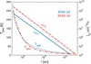Fig. 1

Radial profiles of molecular hydrogen number densities $n_{H_{2}}$ $n_{\mathrm{H}_{2}}$ (cm⁻³) and gas temperature T_gas (K) in NGC 1333-IRAS 2A and NGC 1333-IRAS 4A envelope models. The blue solid line and red dashed line show radial $n_{H_{2}}$ $n_{\mathrm{H}_{2}}$ profiles in IRAS 2A and IRAS 4A envelope models, respectively. The blue dotted line and red dash-dotted line show radial T_gas profiles in IRAS 2A and IRAS 4A envelope models, respectively.

2.1.2 X-ray fields

The observed X-ray spectra from Young Stellar Objects (YSOs) are usually fitted with the emission spectrum of a thermal plasma (e.g., Hofner & Churchwell 1997; Stäuber et al. 2005; Bruderer et al. 2009). The thermal X-ray spectrum can be approximated with $F_{X, in} (E, r) = F_{0} (r) \exp (- E / k T_{X}) (photons s^{-1} {cm}^{-2} {eV}^{-1}),$ $\begin{equation*} F_{\mathrm{X, in}}(E,r)\,{=}\,F_{0}(r)\exp(-E/kT_{\mathrm{X}}) \ \ \mathrm{(photons \ s^{-1} \, cm^{-2} \, eV^{-1}),} \end{equation*}$ (1)

where r is the radius in the envelope from the central protostar, F_X,in(E, r) is the incident X-ray flux per unit energy, k is the Boltzmann constant, and T_X is the temperature of the X-ray emitting plasma. The factor F₀(r) can be calculated from the following equation, $\begin{array}{l} L_{X} & = & 4 π r^{2} \int_{E_{min}}^{E_{max}} F_{X, in} (E, r) E d E (erg s^{-1}) \\ = & 4 π r^{2} \int_{E_{min}}^{E_{max}} F_{0} (r) \exp (- E / k T_{X}) E d E (erg s^{-1}), \end{array}$ $\begin{eqnarray*} L_{\mathrm{X}}&\,{=}\,&4\pi r^{2}\int_{E_{\mathrm{min}}}^{E_{\mathrm{max}}} F_{\mathrm{X, in}}(E,r)E \mathrm{d}E \ \ \mathrm{(erg \, s^{-1})} \\ &\,{=}\,&4\pi r^{2}\int_{E_{\mathrm{min}}}^{E_{\mathrm{max}}} F_{0}(r)\exp(-E/kT_{\mathrm{X}}) E \mathrm{d}E \ \ \mathrm{(erg \, s^{-1})}, \end{eqnarray*}$

where L_X is the X-ray luminosity of the central protostar. The local (attenuated) X-ray flux per unit energy F_X (E, r) is given by $F_{X} (E, r) = F_{X, in} (E, r) \exp (- τ (E, r)),$ $\begin{equation*} F_{\mathrm{X}}(E,r)\,{=}\,F_{\mathrm{X, in}}(E,r)\exp(-\tau(E,r)), \end{equation*}$ (4)

where τ(E, r) is the total optical depth from the central protostar position to r. The energy-integrated total attenuated X-ray flux F_X(r) at radius r of the envelope is given by the following equation. 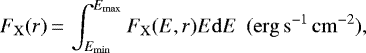$F_{X} (r) = \int_{E_{min}}^{E_{max}} F_{X} (E, r) E d E (erg s^{-1} {cm}^{-2}),$ $\begin{equation*} F_{\mathrm{X}}(r)\,{=}\,\int_{E_{\mathrm{min}}}^{E_{\mathrm{max}}}F_{\mathrm{X}}(E,r)E \mathrm{d}E \ \ \mathrm{(erg \, s^{-1} \, cm^{-2})}, \end{equation*}$ (5)

and τ(E, r) is determined by $τ (E, r) = τ_{p} (E, r) + τ_{c} (E, r),$ $\begin{equation*} \tau(E,r)\,{=}\,\tau_{\mathrm{p}}(E,r)+\tau_{\mathrm{c}}(E,r), \end{equation*}$ (6)

where τ_p(E, r) and τ_c(E, r) are the optical depths determined by photoabsorption and incoherent Compton scattering of hydrogen (Nomura et al. 2007). We note that the attenuation of the X-rays is mainly determined by photoabsorption especially at E < 10 keV, and the influence of Compton scattering of hydrogen on the chemistry is negligible (Stäuber et al. 2005; Bruderer et al. 2009).

Assuming that the photoabsorption cross section of an atom is equal to its photoionization cross section, τ_p (E, r) is obtained by the equation 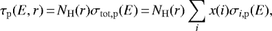$τ_{p} (E, r) = N_{H} (r) σ_{tot, p} (E) = N_{H} (r) \sum_{i} x (i) σ_{i, p} (E),$ $\begin{equation*} \tau_{\mathrm{p}}(E,r)\,{=}\,N_{\mathrm{H}}(r)\sigma_{\mathrm{tot,p}}(E)\,{=}\,N_{\mathrm{H}}(r)\sum_{i} x(i)\sigma_{i\mathrm{,p}}(E), \end{equation*}$ (7)

where N_H(r) is the total hydrogen column density from the central protostar position to r, and σ_tot,p(E) is the total photoabsorption cross section given by the sum of the photoionization cross sections for each element σ_i,p (E) multiplied by its fractional abundance x(i). We calculate the values of σ_i,p(E) using the analytical method in Verner et al. (1993), as done in Walsh et al. (2012). The value of τ_c (E, r) is obtained by the following equation, $τ_{c} (E, r) = N_{H} (r) σ_{c} (E),$ $\begin{equation*} \tau_{\mathrm{c}}(E,r)\,{=}\,N_{\mathrm{H}}(r)\sigma_{\mathrm{c}}(E), \end{equation*}$ (8)

where σ_c(E) is the incoherent Compton scattering cross section of hydrogen. We adopted the values of σ_c (E) from the NIST/XCOM database (Berger et al. 1999).

In Class I and II protostars, the values of observed X-ray luminosities are typically around L_X ~ 10²⁸–10³¹ erg s⁻¹ (Imanishi et al. 2001; Preibisch et al. 2005; Güdel & Nazé 2009). However, the values of L_X in low-mass Class 0 protostars have not yet been well determined (e.g., Hamaguchi et al. 2005; Forbrich et al. 2006; Giardino et al. 2007; Güdel & Nazé 2009; Kamezaki et al. 2014; Grosso et al. 2020), since the X-rays from the central Class 0 protostars are absorbed by their surrounding dense envelopes. Recently, Grosso et al. (2020) reported a powerful X-ray flare from the Class 0 protostar HOPS 383 with L_X ~ 4 × 10³¹ erg s⁻¹ in the 2–8 keV energy band. Takasao et al. (2019) discussed from their simulations that protostar X-ray flares occur repeatedly (approximately every 10 days) even in Class 0 protostars without magnetospheres. These flares are thought to occur when a portion of the large-scale magnetic fields, which are transported by accretion, are removed from the protostar as a result of magnetic reconnection. Stäuber et al. (2007) discussed the X-ray strengths from CN, CO⁺, and SO⁺ abundances, and they estimated that values of L_X in Class 0 low-mass protostars are around 10²⁹ –10³² erg s⁻¹, which are comparable to those in low-mass Class I protostars. However, Benz et al. (2016) discussed that the abundances of CN and CO⁺ obtained by Herschel/HIFI observations can also be explained by FUV irradiation of outflow cavity walls (see also Bruderer et al. 2010), and suggested that the spatial resolution at scales of a few ×10³ au is not sufficient to detect molecular tracers of X-rays. Benz et al. (2016) also estimated the X-ray luminosities from the upper limits of H₃O⁺ line fluxes obtained with Herschel/HIFI toward some low-mass protostars (L_X< 10³⁰ erg s⁻¹ in the Class 0 object IRAS 16293-2422 and L_X ≳ 10³¹ erg s⁻¹ in the Class I object TMC1).

In order to investigate the dependence of the chemical evolution on the strength of the X-ray field, we take values of L_X = 0, 10²⁷, 10²⁸, 10²⁹, 10³⁰, 10³¹, and 10³² erg s⁻¹. We adopt kT_X = 2.6 keV (= 3 × 10⁷ K), which is similar to Stäuber et al. (2006), and is also consistent with typical Class I protostars (Imanishi et al. 2001; Preibisch et al. 2005). We set E_min = 0.1 keV and E_max = 100 keV to cover a sufficient range of X-rays in our calculations. According to Maloney et al. (1996), Stäuber et al. (2005), and Bruderer et al. (2009), the shape of the X-ray spectrum will vary for different values of kT_X, for example with 10⁷ –10⁸ K. However, they discussed that the calculated abundances differ by a factor of a few at most for the different X-ray temperatures, and that the influence of the X-ray luminosities on the chemistry is dominant. We note that we assumed a constant value of X-ray luminosity during 10⁵ year since protostellar X-ray flares repeatedly occur, and as a first step we wanted to know the overall influence of X-ray fields on chemistry (see also Sect. 4.7).

In our calculations the FUV radiation field from the central protostar is neglected. According to Stäuber et al. (2007), X-rays are thought to be more effective for chemistry than FUV fields in the low-mass protostellar envelopes. Low-mass protostars (L_bol ~ 10¹⁻² L_⊙, T_eff < 10⁴ K) emit far fewer UV photons than high-mass protostars (L_bol ~ 10⁴⁻⁵ L_⊙, T_eff ≳ a few × 10⁴ K) due to their lower surface temperatures. Thus, FUV photons from the central source are not effective in destroying molecules in Class 0 protostellar envelopes (Stäuber et al. 2005, 2006). Some FUV radiation from the disk-star boundary can escape through outflow cavities, but only affects a narrow layer along the cavity walls (Visser et al. 2012).

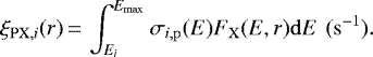
The top panels of Fig. 2 show the radial profiles of F_X (r) in the IRAS 2A and IRAS 4A envelope models. In both models the values of F_X (r) in the innermost region are around 2 × 10⁻⁴ erg s⁻¹ cm⁻² in the case of L_X = 10²⁷ erg s⁻¹, and around 20 erg s⁻¹ cm⁻² in the case of L_X = 10³² erg s⁻¹. In the outer envelopes, the values of F_X (r) reduce because of the increasing values of N_H (r). Compared with the IRAS 2A model, F_X (r) of the IRAS 4A model is lower in the outer regions due to higher densities (see also Fig. 1). The values of F_X (r) at r ~ 10³ au are ~ 1 ×10⁻⁷ erg s⁻¹ cm⁻² (IRAS 2A) and ~ 6 × 10⁻⁸ erg s⁻¹ cm⁻² (IRAS 4A) in the case of L_X = 10²⁷ erg s⁻¹, and ~ 1 × 10⁻² erg s⁻¹ cm⁻² (IRAS 2A) and ~ 6 × 10⁻³ erg s⁻¹ cm⁻² (IRAS 4A) in the case of L_X = 10³² erg s⁻¹.

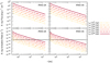Fig. 2

Radial profiles of the X-ray flux F_X(r) (erg s⁻¹ cm⁻²) (top panels) and the secondary X-ray ionization rate ξ_X(r) (s⁻¹) (bottom panels) in NGC 1333-IRAS 2A (left) and NGC 1333-IRAS 4A (right) envelope models. In the bottom panels, the horizontal gray solid lines show the assumed constant cosmic-ray ionization rate ξ_CR (r) = 1.0 × 10⁻¹⁷ s⁻¹. In all panels the different line styles and colors in the radial F_X(r) and ξ_X (r) profiles denote models with different central star X-ray luminosities L_X.

2.2 Calculations of chemical evolution

We calculated the chemical evolution of low-mass Class 0 protostellar envelopes using a detailed gas-grain chemical reaction network including X-ray-induced chemical processes (Walsh et al. 2012, 2015). We note that Stäuber et al. (2005, 2006) focused on gas-phase water chemistry only. In order to investigate the radial dependence of the abundances of both gas and ice molecules on X-ray fields, we included gas-phase reactions, thermal and non-thermal gas-grain interactions, and grain-surface reactions, simultaneously.

The chemical reaction network adopted in this work is based on the chemical model from Walsh et al. (2015), as also used in Eistrup et al. (2016, 2018), and Bosman et al. (2018b). The detailed background theories and procedures are also discussed in these papers and our previous works (e.g., Walsh et al. 2010, 2012, 2014a,b; Heinzeller et al. 2011; Notsu et al. 2016, 2017, 2018), although there are some differences between these studies and our paper. Here we provide a summary and describe an important update of our adopted chemical reaction network in this paper. Consistent with Stäuber et al. (2006), the chemical evolution in envelopes is run for 10⁵ yr, which is the typical age of Class 0 protostars.

2.2.1 Gas-phase reactions

Our gas-phase chemistry is the complete network from the recent release of the UMIST Database for Astrochemistry (UDfA), called RATE12, and is publicly available⁵ (McElroy et al. 2013). RATE12 includes gas-phase two-body reactions, photodissociation and photoionization, direct cosmic-ray ionization, and cosmic-ray-induced photodissociation and photoionization. Since the FUV radiation fields from the central protostar are neglected in our calculations (see also Sect. 2.1.2), the photodissociation and photoionization by FUV radiation is not included. In contrast, we supplemented this gas-phase network with direct X-ray ionization reactions, and X-ray-induced photoionization and photodissociation processes (see Walsh et al. 2012, 2015, and Sect. 2.2.4 in this paper). In these X-ray-induced photoreactions UV photons are generated internally via the interaction of secondary electrons (produced by X-rays; see also Sect. 2.2.4) with H₂ molecules (Gredel et al. 1987, 1989). As in Walsh et al. (2015), we also added a set of three-body reactions and “hot” H₂ chemistry, although they were not expected to be important at the densities and temperatures calculated in this study. Moreover, the gas phase chemical network is supplemented with reactions for important species, for example the CH₃O radical, which are not included in RATE12. The gas-phase formation and destruction reactions for these species are from the Ohio State University (OSU) network (Garrod et al. 2008).

Table 1

UV photodesorption yields.

2.2.2 Gas–grain interactions

In our calculations we consider the freezeout of gas-phase molecules on dust grains, and the thermal and non-thermal desorption of molecules from dust grains (Hasegawa et al. 1992; Walsh et al. 2010, 2012, 2014a, 2015; Notsu et al. 2016). The adopted non-thermal desorption mechanisms are cosmic-ray-induced (thermal) desorption (Leger et al. 1985; Hasegawa & Herbst 1993; Hollenbach et al. 2009), reactive desorption (see Sect. 2.2.3), and photodesorption. We note that the direct cosmic-ray-induced desorption has no significant impact on chemistry, since its reaction timescale is typically much longer (≫ 10⁷ yr) than the age of protostars (Hollenbach et al. 2009).

We include photodesorption by both external X-ray photons and UV photons generated internally via the interaction of secondary electrons produced by cosmic rays with H₂ molecules. Following Walsh et al. (2015), we assume compact spherical grains with a radius a of 0.1 μm and a fixed density of ~10⁻¹² relative to the gas number density. We adopt a value for the integrated cosmic-ray-induced UV photon flux as 10⁴ photons cm⁻² s⁻¹ (Prasad & Tarafdar 1983; Walsh et al. 2014a). We scale the internal UV photon flux by the cosmic-ray ionization rate.

We use experimentally determined photodesorption yields, Y_des(j), where available (e.g., Öberg et al. 2007, 2009a,b; Bertin et al. 2016; Cuppen et al. 2017). These experiments were conducted by using UV lamps that mimic well the FUV radiation field (100−200 nm) produced locally by H₂ emission excited by cosmic-rays or X-rays. For all species without experimentally determined photodesorption yields, a value of 10⁻³ molecules photon⁻¹ is used. The values of photodesorption yields adopted in our work are the same as those in Walsh et al. (2015), except the value of CH₃OH. Recent studies into methanol ice photodesorption showed that methanol does not desorb intact at low temperatures (e.g., Bertin et al. 2016; Cruz-Diaz et al. 2016), and the value of the intact photodesorption yield for CH₃OH is thought to be much lower (~ 10⁻⁶–10⁻⁵) than that in the previous estimates (~10⁻³, Öberg et al. 2009c). The values of photodesorption yields adopted in this work, Y_des(j), are listed in Table 1. On the basis of Öberg et al. (2009b), Arasa et al. (2010, 2015), Bertin et al. (2016), Cruz-Diaz et al. (2016), and Walsh et al. (2018), we include the fragmentation pathways for water ice (50% H₂O and 50% OH+H) and methanol photodesorption (e.g., 85.0% CO+H₂+H₂, 6.1% CH₃OH, 4.85% H₂CO+H₂, 3.0% CH₃+OH). The values of Y_des(j) for H₂O and CH₃OH listed in Table 1 are the sum of all of these fragmentation pathways. The adopted value of intact photodesorption yield for CH₃OH is 1.5 × 10⁻⁵ (molecules photon⁻¹) and 6.1% of Y_des(j) for CH₃OH.

As in Walsh et al. (2014a), we treat X-ray-induced photodesorption as we treat UV photodesorption, and assume the same photodesorption yields for both X-ray-induced photodesorption and UV photodesorption. In addition, following Walsh et al. (2014a), we do not include the photodesorption by UV photons generated internally via the interaction of secondary electrons produced by X-rays with H₂ molecules because the experimental constraints for X-ray-induced photodesorption are limited, and the interaction of X-ray photons with ice is still not clearly understood (for more details, see, e.g., Andrade et al. 2010; Walsh et al. 2014a). In Sects. 4.2 and 4.3 we discuss the rates of X-ray-induced photodesorption in detail, by conducting additional test calculations. We note that we also allow X-rays to photodissociate grain mantle material (see also Sect. 2.2.3 and Walsh et al. 2014a), in which UV photons are generated internally via the interaction of secondary electrons (produced by X-rays; see Sect. 2.2.4) with H₂. Recently, Dupuy et al. (2018) and Basalgète et al. (2021a,b) experimentally investigated X-ray-induced photodesorption rates of H₂O, O₂, CH₃OH, and other related molecules (for more details, see Sect. 4.3).

The sticking coefficient is assumed to be 1 for all species, except for H, which leads to H₂ formation (for more details, see Appendix B.2 of Bosman et al. 2018b). Compared with Walsh et al. (2015) the values of molecular binding energies, E_des(j), are updated on the basis of the recent extensive literature review performed by Penteado et al. (2017) and grain-surface chemistry review by Cuppen et al. (2017). The values of binding energies for several important molecules, E_des(j), are listed in Table 2.

Table 2

Initial abundances for dominant molecules in our protostellar envelope models and their binding energies.

2.2.3 Grain-surface reactions

For the grain-surface reactions we use the reactions included in the Ohio State University (OSU) network (Garrod et al. 2008). In addition to grain-surface two-body reactions and reactive desorptions, grain-surface cosmic-ray-induced and X-ray-induced photodissociations are also included in our calculations (Garrod et al. 2008; Walsh et al. 2014a, 2015). In these X-ray-induced photodissociation reactions, UV photons are generated internally via the interaction of secondary electrons (produced by X-rays; see also Sect. 2.2.4) with H₂ molecules (Gredel et al. 1987, 1989). In addition, as Walsh et al. (2018) adopted, we include an extended grain-surface chemistry network for methanol and its related compounds from Woods et al. (2013) and Chuang et al. (2016). Moreover, we have also added the hydrogenation abstraction pathway during hydrogenation from HNCO to NH₂CHO (Noble et al. 2015). As in Walsh et al. (2015) and Bosman et al. (2018b), the additional water formation routes studied by Cuppen et al. (2010) and Lamberts et al. (2013) are also included. The grain-surface two-body reaction rates are calculated assuming the Langmuir-Hinshelwood mechanism only, and using the rate equation method as described in Hasegawa et al. (1992). Only the top two monolayers of the ice mantle are chemically active. We assume that the size of the barrier to surface diffusion is 0.3 × E_des(j) (Walsh et al. 2015). For the lightest reactants, H and H₂, we adopt either the classical diffusion rate or the quantum tunnelling rate depending on which is fastest (Hasegawa et al. 1992; Bosman et al. 2018b). For the quantum tunnelling rates, we adopt a rectangular barrier of width 1.0 Å (Hasegawa et al. 1992; Bosman et al. 2018b). As in Bosman et al. (2018b), reaction-diffusion competition for grain-surface reactions with a reaction barrier (Garrod & Pauly 2011) is not included.

We note that grain-surface reactions take place on finite grain surfaces, where the populations of certain chemical species can become very small (≪1). If surface reactions occur very quickly in such a regime (the stochastic limit situation), the reaction rates might be overestimated compared with the actual values (Garrod 2008; Garrod & Pauly 2011; Cuppen et al. 2017). Such stochastic effects would be more important on the smaller dust grains (such as a ≲ 0.1μm), since the number of surface sites per grain is smaller (Barzel & Biham 2007; Garrod 2008). Stantcheva & Herbst (2004) and Vasyunin et al. (2009) showed that the stochastic effects are most important on chemical evolution in moderately warm regions (T_dust ~ 30 K), and that the abundances of molecules such as H₂O and CO₂ can differ by more than an order of magnitude. In contrast, they also showed that these effects are not important in the regions with low (T_dust ≲ 10 K) and high (T_dust ≳ 50 K) temperatures (see also Caselli et al. 1998). Compared with the physical structures shown in Fig. 1, the molecular abundances just outside the water snowline (r ~ (1–3) × 10² au) will not be strongly influenced by such effects. In addition, the sizes of dust grains in protostellar envelopes are on average larger than 0.1 μm (Ormel et al. 2009; Miotello et al. 2014; Li et al. 2017), and thus the effects would be smaller than those in diffuse clouds. The micro- and macroscopic Monte Carlo techniques would be helpful for much more precise treatment of the grain-surface chemistry (e.g., Tielens & Hagen 1982; Vasyunin et al. 2009; Vasyunin & Herbst 2013; Garrod et al. 2009; Cuppen et al. 2017).

2.2.4 X-ray ionization rates

We include a set of gas-phase and grain-surface X-ray-induced reactions which we duplicate from the existing set of cosmic-ray-induced reactions contained in RATE12 (McElroy et al. 2013; Walsh et al. 2015). The reaction rates are estimated by scaling the cosmic-ray-induced reaction rates by the ratio of the local X-ray ionization rate ξ_X (r) and cosmic-ray ionization rate ξ_CR(r).

In this study, we calculate the secondary X-ray ionization rate at each radius ξ_X (r) via the following equation (see also Glassgold et al. 1997; Walsh et al. 2012), $ξ_{X} (r) = \sum_{i} \int_{E_{i}}^{E_{max}} x (i) σ_{i, p} (E) F_{X} (E, r) (\frac{E - E_{i}}{Δ ϵ}) d E (s^{-1}),$ $\begin{equation*} \xi_{\mathrm{X}}(r)\,{=}\,\sum_{i} \int_{E_{i}}^{E_{\mathrm{max}}} x(i)\sigma_{i\mathrm{,p}}(E)F_{\mathrm{X}}(E,r)\left(\frac{E-E_{i}}{\Delta\epsilon}\right) \mathrm{d}E \ \ \mathrm{(s^{-1})}, \end{equation*}$ (9)

where E_i is the ionization potential foreach element i, and x(i), σ_i,p (E), and F_X (E, r) are determined as described in Sect. 2.1.2. The number of secondary ionizations per unit energy produced by primary photoelectrons is given by the expression (E − E_i)∕Δϵ, where Δϵ = 37 eV is the mean energy required to make an ion pair. X-rays interact only with atoms, regardless of whether an atom is bound within a molecule or is free (Glassgold et al. 1997). According to Maloney et al. (1996), these secondary ionization rates ξ_X (r) dominate the total ionization rates in X-ray dissociation regions. For atoms heavier than Li, inner-shell ionization is followed by the Auger effect, in which the excited, photo-produced ion undergoes two- or even three-electron decay (Glassgold et al. 1997). Our calculations do not include the Auger effect. According to Igea & Glassgold (1999) and Stäuber et al. (2005), the Auger electrons and the primary photoelectron are negligible compared to the secondary electrons for the ionization of the gas.

In this study we adopt a constant value for the cosmic-ray ionization rate of ξ_CR (r) = 1.0 × 10⁻¹⁷ s⁻¹ at all radii (Umebayashi & Nakano 2009). The bottom panels of Fig. 2 show the radial profiles of the X-ray ionization rate ξ_X (r) in the IRAS 2A and IRAS 4A envelope models. In both models the values of ξ_X (r) in the innermost region are around 10⁻¹⁷ s⁻¹ in the case of L_X = 10²⁷ erg s⁻¹, and around 10⁻¹² s⁻¹ in the case of L_X = 10³² erg s⁻¹. In the outer envelopes the values of ξ_X(r) are reduced because of increasing values of N_H(r). Compared with the IRAS 2A model, ξ_X(r) of the IRAS 4A model is lower in the outer regions due to higher densities (see also Fig. 1). The values of ξ_X (r) at r ~ 10³ au are ~ 10⁻²¹ s⁻¹ (IRAS 2A) and ~ 10⁻²² s⁻¹ (IRAS 4A) in the case of L_X = 10²⁷ erg s⁻¹, and ~ 10⁻¹⁶ s⁻¹ (IRAS 2A) and ~ 10⁻¹⁷ s⁻¹ (IRAS 4A)in the case of L_X = 10³² erg s⁻¹. In regions with ξ_X(r) > ξ_CR(r) (= 1.0 × 10⁻¹⁷ s⁻¹), X-ray-induced photoionization and photodissociation processes are considered to be dominant compared with cosmic-ray-induced photoionization and photodissociation processes. In the cases of L_X ≳ 10³¹ erg s⁻¹, the values ofξ_X(r) are larger than that of ξ_CR(r) at r ≲ 10³ au in the IRAS 2A model and r ≲ 5 × 10² au in the IRAS 4A model. Inside the water snowline (r < 10² au), the values ofξ_X(r) are larger than that of ξ_CR(r) in the cases of L_X > 10²⁹ erg s⁻¹ for IRAS 2A and L_X > 10³⁰ erg s⁻¹ for IRAS 4A.

We also included the direct (primary) X-ray ionization of elements. The reaction rate ξ_{PX, i}(r) for each element i is given by the following equation (Verner et al. 1993; Walsh et al. 2012): $ξ_{PX, i} (r) = \int_{E_{i}}^{E_{max}} σ_{i, p} (E) F_{X} (E, r) d E (s^{-1}) .$ $\begin{equation*} \xi_{\mathrm{PX,} i}(r)\,{=}\,\int_{E_{i}}^{E_{\mathrm{max}}}\sigma_{i\mathrm{,p}}(E)F_{\mathrm{X}}(E,r) \mathrm{d}E \, \ \mathrm{(s^{-1})}. \end{equation*}$ (10)

2.2.5 Initial abundances

To generate a set of initial abundances for input into protostellar envelope models, we run a dark cloud model (T_gas = T_dust = 10 K, $n_{H_{2}} = 10^{4}$ $n_{\mathrm{H}_{2}}\,{=}\,10^{4}$ cm⁻³, ξ_CR (r) = 1.0 × 10⁻¹⁷ s⁻¹). As Walsh et al. (2015) adopted, the values of volatile elemental abundances for O, C, and N are respectively 3.2 × 10⁻⁴, 1.4 × 10⁻⁴, and 7.5 × 10⁻⁵ relative to total hydrogen nuclei density. These values are based on diffuse cloud observations (Cardelli et al. 1991, 1996; Meyer et al. 1998). For other elements, we use the low-metalallicity elemental abundances from Graedel et al. (1982). In this way we begin the envelope calculations with an ice reservoir on the grain mantle built up in the dark cloud and pre-stellar core phases. We use initial abundances at a time of 3.2 × 10⁵ yr on the basis of Walsh et al. (2015) and Drozdovskaya et al. (2016), except for the values of O gas, O₂ gas, and H₂O ice, which we treat as free parameters in our study but such that elemental oxygen abundance is preserved at 3.2 × 10⁻⁴. This timescale of 3.2 × 10⁵ yr is consistent with the observed pre-stellar core lifetime of ~(2−5) × 10⁵ years (Enoch et al. 2008).

In the above calculation under the dark cloud condition, the abundances with respect to total hydrogen nuclei density of O gas, O₂ gas, and H₂O ice at a time of 3.2 × 10⁵ yr are 8.5 × 10⁻⁵, 2.2 × 10⁻⁶, and 1.1 × 10⁻⁴. If we consider longer time evolution (≳10⁶ yr), however, the abundances of O gas and O₂ gas become much smaller (≪10⁻⁶; see also Yıldız et al. 2013; Taquet et al. 2018) and the abundance of H₂O ice becomes higher (~2 × 10⁻⁴, see also Schmalzl et al. 2014).

Previous chemical calculations (e.g., Walsh et al. 2015; Eistrup et al. 2016, 2018; Drozdovskaya et al. 2016) adopted a similarly high abundance for H₂O ice (~(1−3) × 10⁻⁴), and low or zero abundances for O and O₂ gas as initial conditions. Thus, here we assume that all oxygen atoms in these three species are incorporated into H₂O ice (= 1.984 × 10⁻⁴).

Observations show that H₂O ice is indeed a major oxygen carrier in dark clouds and pre-stellar cores, although measured water ice abundances are consistently a factor of 2–4 below the expected value of 2 × 10⁻⁴ if all volatile oxygen that is not contained in CO is in water ice (Öberg et al. 2011; Boogert et al. 2015). Chemical modeling of Schmalzl et al. (2014) and Furuya et al. (2016) show that the water ice abundance in pre-stellar cores increases with pre-collapse time (see also van Dishoeck et al. 2021), and that such a low water ice abundance can only be obtained for a short pre-stellar period. At pre-collapse times of t_pre < 10⁶ yr, a considerableamount of oxygen is also found in other oxygen-bearing species (mainly O in addition to CO). At t_pre ≳ 10⁶ yr, oxygen returns into the water network and water ice then becomes the dominant oxygen reservoir (up to ~ 2 × 10⁻⁴) with CO.

The observed low water ice abundances with respect to hydrogen nuclei of low-mass protostellar envelopes of ~ (3−8) × 10⁻⁵ would require short pre-collapse lifetimes of t_pre ≲ 10⁵ yr (Schmalzl et al. 2014), less than the observed pre-stellar core lifetimes of ~ (2−5) × 10⁵ yr (Enoch et al. 2008). In addition, this shorter pre-collapse phase is inconsistent with the discussions in Yıldız et al. (2013) who argued for a long pre-collapse phase of at least 10⁶ yr to explain the lower upper limit of gas-phase cold O₂ abundances (≫10⁻⁶) toward IRAS 4A (see also Taquet et al. 2018). Possible mitigations include the possibility that a fraction of water ice is locked up in larger (micron-sized) dust grains that do not contribute to the infrared water ice bands, or the presence of some amount of unidentified depleted oxygen (UDO), which has also been invoked to explain the oxygen budget in diffuse clouds (Whittet 2010; Schmalzl et al. 2014; van Dishoeck et al. 2021). Here we do not consider either of these two options.

The fractional abundances with respect to total hydrogen nuclei density for dominant and important molecules, which are used as initial abundances in our protostellar envelope models, are listed in Table 2.

3 Results

3.1 Water fractional abundances

Figure 3 shows the radial profiles of the water gas fractional abundances with respect to total hydrogen nuclei densities $n_{H_{2} O}$ $n_{\mathrm{H}_{2}\mathrm{O}}$ /n_H in IRAS 2A(left panels) and IRAS 4A (right panels) envelope models, for the various X-ray luminosities (L_X = 0, 10²⁷, 10²⁸, 10²⁹, 10³⁰, 10³¹, and 10³² erg s⁻¹). Figure 4 shows the radial profiles of water ice fractional abundances $n_{H_{2} O, ice}$ $n_{\mathrm{H}_{2}\mathrm{O}, \mathrm{ice}}$ /n_H in the same models. In both models the water snowline positions are at r ~ 10² au, where T_gas is around 100 K.

For L_X = 0 erg s⁻¹, water gas abundances are around 2 × 10⁻⁴ inside the water snowline (T_gas > 10² K, r < 10² au), and sharply decrease to ≲10⁻¹⁰ just outside the water snowline (T_gas < 10² K, r > 10² au). The water gas abundances increase in the outer low-density envelopes ( $n_{H_{2} O}$ $n_{\mathrm{H}_{2}\mathrm{O}}$ /n_H ~ 10⁻⁷ at r ~ 10⁴ au) since in this region the water abundances are mainly determined by the balance between the freeze-out of water vapor and the cosmic-ray-induced photodesorption of water ice, which maintains an approximately constant number density of gas phase water (for more details, see Schmalzl et al. 2014).

Outside the water snowline, for L_X ≳ 10³⁰ erg s⁻¹, water gas abundances become higher (up to $n_{H_{2} O}$ $n_{\mathrm{H}_{2}\mathrm{O}}$ /n_H ~ 10⁻⁸–10⁻⁷), compared with the values ( $n_{H_{2} O}$ $n_{\mathrm{H}_{2}\mathrm{O}}$ /n_H ~ 10⁻¹⁰) for L_X ≲ 10²⁷ erg s⁻¹ in IRAS 2A and L_X ≲ 10²⁸ erg s⁻¹ in IRAS 4A. In addition, water ice abundances (see Fig. 4) are around 2 × 10⁻⁴ outside the water snowline for L_X ≲ 10³⁰ erg s⁻¹, and they become much lower (below to $n_{H_{2} O}$ $n_{\mathrm{H}_{2}\mathrm{O}}$ /n_H ~ 10⁻⁸ at a few × 10² au) for L_X ≳ 10³¹ erg s⁻¹. We conclude that photodesorption by external X-ray photons (e.g., Walsh et al. 2015; Cuppen et al. 2017; Dupuy et al. 2018) is important in this region (see also Sects. 4.2 and 4.3). This X-ray effect is stronger in the IRAS 2A model since it has around a 3–6 times lower density and thus higher X-ray fluxes (see Fig. 2) than the IRAS 4A model. The lower density in the IRAS 2A also decreases the efficacy of two-body ion-molecule reactions (see Appendix A where we demonstrate the effect of density only on the chemistry). Water gas abundances at r ≳ 10³ au are also affected by strong X-ray fluxes, although ξ_X(r) is smaller than ξ_CR(r) in these regions. This occurs because at r ≳ 10³ au the rates of the X-ray-induced photodesorption of water ice are around 10³ times higher than those of cosmic-ray-induced photodesorption, and much higher (> 10²⁰ times) than that of thermal desorption and cosmic-ray-induced (thermal) desorption. The chemical model adopted by Stäuber et al. (2005, 2006) did not include non-thermal desorption processes, and thus they did not find this dependence of the gaseous water abundances on X-ray fluxes outside the water snowline.

Inside the water snowline (T_gas > 10² K, r < 10² au), for L_X ≲ 10²⁹ erg s⁻¹ in IRAS 2A and L_X ≲ 10³⁰ erg s⁻¹ in IRAS 4A, the gas maintains high water abundances of 10⁻⁴, and H₂O is the dominant oxygen carrier along with CO. On the other hand, for L_X ≳ 10³⁰ erg s⁻¹ in IRAS 2A and L_X ≳ 10³¹ erg s⁻¹ in IRAS 4A, water gas abundances become much lower just inside the water snowline (T ~ 100 − 250 K, below to $n_{H_{2} O}$ $n_{\mathrm{H}_{2}\mathrm{O}}$ /n_H ~ 10⁻⁸–10⁻⁷) and in the innermost regions (T ~ 250 K, $n_{H_{2} O}$ $n_{\mathrm{H}_{2}\mathrm{O}}$ /n_H ~ 10⁻⁶).

Within the water snowline water sublimates from the dust-grain surfaces into the gas phase. According to Stäuber et al. (2005, 2006), van Dishoeck et al. (2013, 2014) and Walsh et al. (2015), in the presence of X-rays, gas-phase water in this region is mainly destroyed with X-ray-induced photodissociation (H+OH), and ion-molecule reactions (e.g., with HCO⁺, H⁺, H $_{3}^{+}$ $_{3}^{+}$ , and He⁺). For L_X ≳ 10²⁹ erg s⁻¹ in IRAS 2A and L_X ≳ 10³⁰ erg s⁻¹ in IRAS 4A, the X-ray ionization rates ξ_X(r) are higher than our adopted cosmic ray ionization rate ξ_CR(r) (= 1.0 × 10⁻¹⁷ s⁻¹) within the water snowline (see Fig. 2). Thus, these processes are important to explain the dependence on X-ray fluxes and number densities within the water snowline. Stäuber et al. (2006) discussed that these ion-molecule reactions are more effective than X-ray-induced photodissociation, with resulting water gas abundances varying by less than 15% if they ignored the X-ray-induced photodissociation. In our calculations, we also confirm that the reaction rates of these ion-molecule reactions are higher than those of the X-ray-induced photodissociation leading to H+OH, and that the former reactions become more important compared with the latter reaction as the gas densities become higher (see also Appendix A).

At r ~ 60 au and for L_X = 10³² erg s⁻¹ in the IRAS 2A model, the water gas abundance and $n_{H_{2} O}$ $n_{\mathrm{H}_{2}\mathrm{O}}$ are 1.4 × 10⁻⁷ and 5.9 × 10¹ cm⁻³ at t = 10⁵ yr, respectively, and the HCO⁺ gas abundance and $n_{{HCO}^{+}}$ $n_{\mathrm{HCO}^{+}}$ ⁶ are 9.8 × 10⁻⁹ and 4.0 cm⁻³ at t = 10⁵ yr, respectively. On the basis of these values, the rate coefficient of the ion-molecule reaction with H₂O+HCO⁺ →CO+H₃O⁺, k₁, is ~ 3.7 × 10⁻⁹ cm³ s⁻¹ (Adams et al. 1978), and the reaction rate, R(1) = k₁ $n_{H_{2} O}$ $n_{\mathrm{H}_{2}\mathrm{O}}$ $n_{{HCO}^{+}}$ $n_{\mathrm{HCO}^{+}}$ , is ~ 8.7 × 10⁻⁷ cm⁻³ s⁻¹. In contrast, the rate coefficient of X-ray-induced photodissociation leading to H+OH, k₂, is ~ 8.6 × 10⁻¹¹ s⁻¹ (Gredel et al. 1989), and the reaction rate, R(2) = k₂ $n_{H_{2} O}$ $n_{\mathrm{H}_{2}\mathrm{O}}$ , is ~ 5.1 × 10⁻⁹ cm⁻³ s⁻¹.

We note that for L_X ≳ 10³¹ erg s⁻¹ the abundances of HCO⁺ within the water snowline (≳10⁻⁹, see Sect. 3.3) are higher than those of other molecular ions which are important to water gas destruction such as He⁺ (≲ 10⁻¹⁰). This makes HCO⁺ the most important destructor of H₂O in highly ionized regions.

In the innermost high-temperature region (T_gas ~ 250 K) the following two-body reaction with the reaction barrier of 1736 K (Oldenborg et al. 1992), $OH + H_{2} \to H + H_{2} O,$ $\begin{equation*} \mathrm{OH}+\mathrm{H}_{2}\rightarrow\mathrm{H}+\mathrm{H}_{2}\mathrm{O}, \end{equation*}$ (11)

becomes more efficient, and thus water gas abundances become relatively high ( $n_{H_{2} O}$ $n_{\mathrm{H}_{2}\mathrm{O}}$ /n_H ~ 10⁻⁶) even in the highest X-ray flux cases (L_X = 10³² erg s⁻¹). As Stäuber et al. (2005, 2006) noted, X-ray destruction processes are more effective in lower-density models.

3.2 Molecular and atomic oxygen fractional abundances

Figure 5 presents the radial profiles of the fractional abundances of gaseous molecular oxygen $n_{O_{2}}$ $n_{\mathrm{O}_{2}}$ /n_H and atomic oxygen n_O /n_H in IRAS 2Aand IRAS 4A envelope models, for the various X-ray luminosities. The figure shows that the O₂ abundances at r ≲ 10⁴ au (IRAS 2A) and r ≲ 6 × 10³ au (IRAS 4A), and the O abundance at r ≲ 10³ au increase (within each snowline position) as X-ray luminosities increase. Both molecular and atomic oxygen are very volatile (E_des(O) = 1660 K and E_des(O₂) = 898 K) compared with H₂O (E_des(H₂O) = 4880 K), thus their snowline positions are located in the outer envelopes (r > 5 × 10² au).

Inside the water snowline, both molecular and atomic oxygen abundances are much lower (< 10⁻⁸) in the cases of low X-ray luminosities (L_X ≲ 10²⁸ erg s⁻¹ in IRAS 2A and L_X ≲ 10²⁹ erg s⁻¹ in IRAS 4A). In contrast, for moderate X-ray luminosities (L_X ~ 10²⁹ erg s⁻¹ in IRAS 2A and L_X ~ 10³⁰ erg s⁻¹ in IRAS 4A) and high X-ray luminosities (L_X≳ 10³⁰ erg s⁻¹ in IRAS 2A and L_X ≳ 10³¹ erg s⁻¹ in IRAS 4A), their abundances become larger, and reach about ~ 5 × 10⁻⁵–10⁻⁴ with L_X ≳ 10³¹ erg s⁻¹. Compared with the water gas abundances, both molecular and atomic oxygen have opposite dependence on X-ray fluxes. Thus, the identity of the main volatile oxygen carrier in the inner regions is very sensitive to the X-ray flux from the central protostars (see also Sect. 4.1). In Sects. 3.2–3.7 and 4.1, and Appendices C, D, and E, we adopted the same definition for the values of low, moderate, and high X-ray luminosities.

According to Woitke et al. (2009) and Walsh et al. (2015), in the presence of X-rays, atomic oxygen is mainly produced by X-ray-induced photodissociation of OH and CO. OH is efficiently produced by X-ray-induced photodissociation and fragmental photodesorption of H₂O (see Sect. 3.4), and thus the O abundance increases as X-ray fluxes become larger. In addition, as also discussed in Walsh et al. (2015) and Eistrup et al. (2016), molecular oxygen is formed in the gas-phase via the reaction $O + OH \to O_{2} + H,$ $\begin{equation*}\mathrm{O}+\mathrm{OH}\rightarrow\mathrm{O}_{2}+\mathrm{H}, \end{equation*}$ (12)

and is destroyed via photodissociation and reactions with C and H to yield CO and OH, respectively. We note that reaction (12) is a barrierless neutral-neutral reaction and has a negligible temperature dependence (Carty et al. 2006; Taquet et al. 2016b). The O and OH gas abundances both increase as the X-ray fluxes become larger, and thus the O₂ gas abundances become higher, especially in the inner warm envelope where water is sublimated from dust grains.

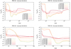Fig. 3

Radial profiles of water gas fractional abundances with respect to total hydrogen nuclei densities $n_{H_{2} O}$ $n_{\mathrm{H}_{2}\mathrm{O}}$ /n_H for the whole envelopes on a log scale (top panels) and the inner regions only (r < 200 au) on a linear scale (bottom panels) in NGC 1333-IRAS 2A (left) and NGC 1333-IRAS 4A (right) envelope models. The double-dashed double-dotted lines, the dashed double-dotted lines, the double-dashed dotted lines, the dash-dotted lines, the dotted lines, the dashed lines, and the solid lines show the radial $n_{H_{2} O}$ $n_{\mathrm{H}_{2}\mathrm{O}}$ /n_H profiles for values of central star X-ray luminosities L_X = 0, 10²⁷, 10²⁸, 10²⁹, 10³⁰, 10³¹, and 10³² erg s⁻¹, respectively. The line color gradually changes from green to yellow, orange, red, and brown as the value of L_X increases. In Figs. 5–7, C.1, C.2, D.1, E.1, H.1, and H.2, we adopt the same line types and color patterns of the calculated radial fractional abundance profiles of gas-phase molecules for different values of L_X.

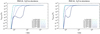Fig. 4

Radial profiles of water ice fractional abundances $n_{H_{2} O, ice}$ $n_{\mathrm{H}_{2}\mathrm{O}, \mathrm{ice}}$ /n_H in NGC1333-IRAS 2A (left panel) and NGC 1333-IRAS 4A (right panel) envelope models. The line color gradually changes from green to cyan, blue, and indigo as the value of L_X increases. The profiles for L_X = 0−10²⁹ erg s⁻¹ almost overlap. In Figs. 7, C.1, and C.2, we adopt the same line types and color patterns of the radial fractional abundance profiles of icy-phase molecules for different values of L_X.

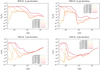Fig. 5

Radial profiles of the gaseous fractional abundances of molecular oxygen $n_{O_{2}}$ $n_{\mathrm{O}_{2}}$ /n_H (top panels) and atomic oxygen n_O/n_H (bottom panels) in NGC 1333-IRAS 2A (left) and NGC 1333-IRAS 4A (right) envelope models.

3.3 HCO⁺ fractional abundances

The top panels of Fig. 6 show the radial profiles of the HCO⁺ fractional abundances $n_{{HCO}^{+}}$ $n_{\mathrm{HCO}^{+}}$ /n_H in IRAS 2A and IRAS 4A envelope models for the various X-ray luminosities. According to our model, the HCO⁺ abundances at r ≳ 10³ au (~ 10⁻⁹–10⁻⁸ for IRAS 2A, and ~ 10⁻¹⁰–10⁻⁹ for IRAS 4A) do not change with different X-ray luminosities. This is consistent with the input assumption that cosmic-ray ionization dominates at these radii (see Fig. 2 and Sect. 4.6).

The HCO⁺ abundances at r ≲ 10³ au are affected by strong X-ray fluxes. For low X-ray luminosities, HCO⁺ abundances drop in the inner envelope, and reach ≲10⁻¹³ within the water snowline, due to the efficient destruction by water (see below). In contrast, for high X-ray luminosities they become higher in the inner envelope, and reach more than 10⁻⁹ (for IRAS 2A) and 10⁻¹⁰ (for IRAS 4A) within water snowline. The overall HCO⁺ abundances are higher and X-ray effects are also stronger in the IRAS 2A model, since it has around 3–6 times lower densities and thus higher X-ray fluxes than the IRAS 4A model has (see Figs. 1 and 2, and Appendix A).

The cation HCO⁺ is considered to be a chemical tracer of the water snowline since its most abundant destroyer in warm dense gas is water via the following reaction (Jørgensen et al. 2013; Visser et al. 2015; van ’t Hoff et al. 2018a; Hsieh et al. 2019; Lee et al. 2020; Leemker et al. 2021): $H_{2} O + {HCO}^{+} \to CO + H_{3} O^{+} .$ $\begin{equation*} \mathrm{H}_{2}\mathrm{O}+\mathrm{HCO}^{+}\rightarrow\mathrm{CO}+\mathrm{H}_{3}\mathrm{O}^{+}. \end{equation*}$ (13)

Thus, a strong decline in HCO⁺ (and its isotopologue H¹³ CO⁺) is expected within the water snowline. van ’t Hoff et al. (2018a) conducted spherically symmetric physical-chemical modeling using the same IRAS 2A temperature and number density model that we adopt (see Sect. 2.1.1 and Fig. 1). Their gas-grain chemical model included gas-phase cosmic-ray-induced reactions, but did not include X-ray-induced chemistry (see, e.g., Taquet et al. 2014). They reported an increase of H¹³ CO⁺ emission just outside the water snowline and a spatial anti-correlation of H¹³ CO⁺ and H₂ ¹⁸ O emission in the envelope around IRAS 2A. The radial profiles of water and HCO⁺ gas abundances in van ’t Hoff et al. (2018a) are similar to those in our model with L_X ≲ 10²⁹ erg s⁻¹. On the basis of our modeling, for high X-ray luminosities the water gas abundance sharply decreases inside the water snowline, and thus HCO⁺ is not efficiently destroyed. Formation of HCO⁺ is dominated by the ion-molecule reaction between H $_{3}^{+}$ $_{3}^{+}$ and CO (Schwarz et al. 2018; van ’t Hoff et al. 2018a; Leemker et al. 2021), and H $_{3}^{+}$ $_{3}^{+}$ is mainly formed by the ionization of H₂. Therefore, the HCO⁺ abundances increase as the X-ray ionization rate increases, and they have relatively radially flat profiles for high X-ray luminosities (see Fig. 6). Thus, our work suggests that HCO⁺ and its isotopologue H¹³ CO⁺ lines cannot be used as tracers of the water snowline position if X-ray fluxes are high and inner water gas is absent. The X-ray ionization rates ξ_X(r) where HCO⁺ loses its efficacy as a water snowline tracer are ≳ 10⁻¹⁶ s⁻¹ (see Fig. 2), which corresponds to L_X ≳ 10³⁰–10³¹ erg s⁻¹, depending on density structures.

In Class II disks, HCO⁺ and its isotopologues are thought to trace X-ray and high cosmic-ray ionization rates with ≳ 10⁻¹⁷ s⁻¹ in the disk surface (Cleeves et al. 2014). According to our calculations, HCO⁺ is the dominant cation in the outer envelopes where the cosmic-ray ionization is dominant (see Fig. 2), and also in the inner envelopes if ξ_X(r) is ≳ 10⁻¹⁶ s⁻¹. Thus, in these cases HCO⁺ line emission can be used to estimate the electron number densities and the ionization rates (see also van ’t Hoff et al. 2018a and Sect. 4.6 of this paper).

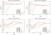Fig. 6

Radial profiles of the gaseous fractional abundances of HCO⁺ $n_{{HCO}^{+}}$ $n_{\mathrm{HCO}^{+}}$ /n_H (top panels) and OH n_OH/n_H (bottom panels) in NGC 1333- IRAS 2A (left) and NGC 1333-IRAS 4A (right) envelope models.

3.4 OH fractional abundances

The bottompanels of Fig. 6 show the radial profiles of the OH gas fractional abundances n_OH /n_H in IRAS 2A (left panel) and IRAS 4A (right panel) envelope models, for the various X-ray luminosities. The OH gas abundances increase at r ≲ 10⁴ au as values of X-ray luminosities become larger. For low X-ray luminosities, the OH gas abundances are around 10⁻⁹–10⁻⁸ at r ≳ 10³ au, and become lower in the inner envelopes (~ 10⁻¹⁰–10⁻⁹ at r ~ 10² au, and ~ 10⁻¹²–10⁻¹¹ at the inner edge). For moderate X-ray luminosities, the OH gas abundances become higher in the inner envelope, and reach more than 10⁻⁹ within the water snowline. In addition, for high X-ray luminosities, the OH gas abundances are much higher at r ~ 10²–10⁴ au (~ 10⁻⁸–10⁻⁶), and become a bit lower (≲10⁻⁸) around and just inside the water snowline (≲10² au).

OH is efficiently produced by X-ray-induced photodissociation of H₂O gas and fragmental photodesorption of H₂O ice (see also Sect. 2.2.2), thus the OH gas abundances increase as the X-ray flux increases (see Sect. 3.1 and Fig. 3). The former X-ray-induced photodissociation reaction is dominant within the water snowline, whereas the fragmental photodesorption reaction is dominant outside the water snowline where a large amount of water ice is present on the dust-grain surface. For example, at r ~ 480 au and L_X = 10³² erg s⁻¹ in the IRAS 2A model, the rate coefficient of the former X-ray-induced photodissociation reaction, k₃, is ~ 5.6 × 10⁻¹³ s⁻¹ (Gredel et al. 1989; Heays et al. 2017), and the reaction rate, R(3) = k₃ $n_{H_{2} O}$ $n_{\mathrm{H}_{2}\mathrm{O}}$ , is ~ 1 × 10⁻¹³ cm⁻³ s⁻¹ at t = 10⁵ yr. In contrast, the rate coefficient of the latter photodesorption reaction, k₄, is ~ 1.9 × 10⁻⁹ (Öberg et al. 2009b; Walsh et al. 2015, see also Sect. 2.2.2), and the reaction rate, R(4) = k₄ $n_{H_{2} O, ice}$ $n_{\mathrm{H}_{2}\mathrm{O}, \mathrm{ice}}$ , is ~ 1 × 10⁻⁹ cm⁻³ s⁻¹ at t = 10⁵ yr. As discussed in Sects. 3.1 and 3.2, atomic oxygen is mainly produced by X-ray-induced photodissociation of OH, and molecular oxygen is produced from OH in the gas phase (O+OH). Therefore, for high X-ray luminosities, the OH gas abundances decrease around and inside the water snowline where molecular and atomic oxygen abundances are high (~10⁻⁴).

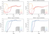Fig. 7

Radial profiles of methanol gas and ice fractional abundances $n_{{CH}_{3} OH}$ $n_{\mathrm{CH}_{3}\mathrm{OH}}$ /n_H (top panels) and $n_{{CH}_{3} OH, ice}$ $n_{\mathrm{CH}_{3}\mathrm{OH},\mathrm{ice}}$ /n_H (bottom panels) in NGC 1333-IRAS 2A (left) and NGC 1333-IRAS 4A (right) envelope models.

3.5 CH₃OH fractional abundances

Figure 7 shows the radial profiles of the methanol gas fractional abundances $n_{{CH}_{3} OH}$ $n_{\mathrm{CH}_{3}\mathrm{OH}}$ /n_H and ice fractional abundances $n_{{CH}_{3} OH, ice}$ $n_{\mathrm{CH}_{3}\mathrm{OH},\mathrm{ice}}$ /n_H in IRAS 2A and IRAS 4A envelope models for the various X-ray luminosities. According to Table 2, the binding energy of CH₃OH is somewhat lower than that of H₂O (E_des(CH₃OH) = 3820 K and E_des(H₂O) = 4880 K), and the CH₃OH snowline position (~2 × 10² au) is located outside the water snowline (~10² au). Thus, CH₃OH is thought to probe the ≳100 K region in hot cores (Nomura & Millar 2004; Garrod & Herbst 2006; Herbst & van Dishoeck 2009; Taquet et al. 2014), and it also provides an outer limit to the water snowline position in protostellar envelopes (e.g., Jørgensen et al. 2013; van ’t Hoff et al. 2018b; Lee et al. 2019, 2020).

The CH₃OH abundances within r ≲ 200 au decrease as the values of X-ray luminosities become larger. Outside the CH₃OH snowline the CH₃OH gas abundances are around 10⁻¹⁰–10⁻⁹ with various X-ray fluxes. Within the CH₃OH and H₂O snowlines, for low X-ray luminosities, the CH₃OH gas abundances are around 10⁻⁷–10⁻⁶. In contrast, for high X-ray luminosities, the CH₃OH gas abundances decrease and reach below 10⁻¹⁶ inside the water snowline.

According to previous studies (e.g., Tielens & Hagen 1982; Watanabe & Kouchi 2002; Cuppen et al. 2009; Fuchs et al. 2009; Drozdovskaya et al. 2014; Furuya & Aikawa 2014; Walsh et al. 2016, 2018; Bosman et al. 2018b; Aikawa et al. 2020), the main pathway to form methanol ice on or within icy mantles of dust grains is CO hydrogenation. Drozdovskaya et al. (2014) discussed the methanol related chemistry both in gas and ice phases, and gas-phase methanol is supplied by the desorption of CH₃OH ice. In our modeling, fragmental X-ray-induced photodesorption reactions are included (see Sect. 2.2.2 of this paper and, e.g., Bertin et al. 2016), and the photofragments of CH₃OH (e.g., CH₃, CH₂OH, CH₃O) will lead to larger and more complex molecules with grain-surface reactions (e.g., Chuang et al. 2016; Drozdovskaya et al. 2016). The gas-phase production via ion-molecule reactions is considered inefficient (Charnley et al. 1992; Garrod & Herbst 2006; Geppert et al. 2006). In the presence of X-rays, gas-phase CH₃OH and other complex organic molecules (COMs) are mainly destroyed by X-ray-induced photodissociation in the inner envelopes (e.g., Garrod & Herbst 2006; Öberg et al. 2009b; Drozdovskaya et al. 2014; Taquet et al. 2016a). Therefore, CH₃OH is not predicted to be an efficient tracer of the warm inner envelope and the water snowline position for moderate and high X-ray luminosities. The X-ray ionization rates ξ_X(r) where CH₃OH loses its efficacy as a water snowline tracer are ≳ a few × 10⁻¹⁷ s⁻¹ (see Fig. 2).

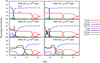Fig. 8

Radial profiles of percentage contributions of the dominant oxygen-bearing molecules to the total elemental oxygen abundance (=3.2 × 10⁻⁴) in the NGC 1333-IRAS 2A envelope model (left panels) and the NGC 1333-IRAS 4A envelope model (right panels). The top, middle, and bottom panels show the radial profiles with L_X = 10²⁸, 10³⁰, and 10³² erg s⁻¹, respectively. The red, blue, purple, black, and green line profiles respectively show the contribution of CO, H₂O, O, O₂, and CO₂ molecules. The solid and dashed line profiles show the contribution of gaseous and icy molecules. Since O₂ and CO₂ include two oxygen atoms per molecule, the percentage contributions are twice as high as those of CO, H₂O, and O whenthey have same fractional abundances with respect to hydrogen nuclei.

3.6 IRAS 4A subgrid envelope models

In Appendix B, Fig. B.1 shows the radial profiles of H₂O, O₂, O, OH, HCO⁺, and CH₃OH gas fractional abundances in the IRAS 4A envelope models, with X-ray luminosities between L_X = 10³⁰ and 10³¹ erg s⁻¹. We plot these subgrid model profiles since there is a large jump in abundances in this X-ray luminosity range (see Figs. 3–7). For the abundance profiles of H₂O, HCO⁺, OH, and CH₃OH gas, between 10³⁰ and 2 × 10³⁰ erg s⁻¹ seems to be the clear boundary. In comparison, the abundance profiles of O₂ and O gas gradually increase in the inner region as the values of L_X increase from 10³⁰ to ~ 6 × 10³⁰ erg s⁻¹.

3.7 Fractional abundances of other dominant oxygen-, carbon-, and nitrogen-bearing molecules

In Figs. C.1, C.2, D.1, and E.1 we show the radial fractional abundances of other dominant oxygen-, carbon-, and nitrogen-bearing molecules (CO₂, CO, CH₄, C₂H, HCN, NH₃, and N₂) for the various X-ray luminosities. According to these figures, as the X-ray flux increases, the fractional abundances of gas-phase CH₄, HCN, and NH₃ decrease within their own snowline positions. The gas-phase CO₂ abundances increase at r ≳ 3 × 10² au (outside the CO₂ snowline) as the X-ray fluxes become larger. At r ≲ 3 × 10² au and for low and moderate X-ray luminosities the CO₂ gas abundance increases as the X-ray fluxes become larger, and they reach ~ 10⁻⁵–10⁻⁴ for moderate X-ray luminosities. In contrast, they decrease for high X-ray luminosities (< 10⁻⁶). In addition, the radial CO and N₂ abundance profiles are constant for the various X-ray luminosities, and they are the dominant carbon and nitrogen carries under the strong X-ray fields. The dependance of radial C₂H gas fractional abundances on X-ray fluxes are much smaller than other dominant molecules. In Appendices C, D, and E more details about the radial abundance profiles are described.

4 Discussion

4.1 Dominant oxygen carriers

Figure 8 shows the radial profiles of percentage contributions of the dominant oxygen-bearing molecules (CO, H₂O, O, O₂, and CO₂) to the total elemental oxygen abundance (=3.2 × 10⁻⁴) in the IRAS2A envelope model and the IRAS 4A envelope model at the various assumed X-ray luminosities (L_X = 10²⁸, 10³⁰, and 10³² erg s⁻¹). Figure 9 shows the pie charts of the percentage contributions of the dominant oxygen-bearing molecules at r ~ 60 au (T_gas ~ 150 K, inside the water snowline) in the IRAS 2A and IRAS 4A envelope models. Table F.1 in Appendix F shows the fractional abundances of major oxygen-bearing molecules at r = 60 au in the IRAS 2A and IRAS 4A envelope models for the various X-ray luminosities, and their percentage contributions. We note that O₂ and CO₂ include two oxygen atoms per molecule, and thus the percentage contributions are twice as high as those of CO, H₂O, and O when they have same fractional abundances with respect to hydrogen nuclei. On the basis of Figs. 8 and 9, and Table F.1, for low X-ray luminosities the H₂O and CO molecules are the dominant oxygen carriers (>90%), both in gas and ice. The percentage contributions of H₂O gas and ice are ≳60%, and that of CO gas and ice are ≳30% throughout the envelopes.

As the X-ray fluxes increase, the abundances of H₂O gas decrease at r ≲ 10² au, and those of H₂O ice also decrease just outside the water snowline (r ≳ 10² au) where the X-ray-induced photodesorption is considered to be efficient (see also Sect. 3.1). Moreover, as the X-ray fluxes increase, the abundances of O₂ and O gas increase in the inner envelopes (inside and just outside the water snowline, see also Sect. 3.2). For high X-ray luminosities, the water gas abundances at r ≲ 10² au become much smaller (≫10⁻⁶), and O₂ and O gas are the dominant oxygen carriers along with CO at r ≲ a few ×10² au. In these cases, the percentage contributions of O₂, O, and CO gas at these radii are ≈40%, ≲ 20%, and ≳ 40%, respectively. In the outer envelopes where the X-ray-induced photodesorption of water is not efficient, H₂O ice and CO gas and ice molecules are still dominant oxygen carriers. In addition, the percentage contributions of CO₂ gas or ice are around 10–40% for moderate X-ray luminosities and around 10–20% for high X-ray luminosities in the regions where the contributions of O₂ gas and H₂O are similar. As discussed in Sect. 3.7 and Appendix C, CO₂ gas abundances at r ≲ 3 × 10² au are highest (up to ~ 10⁻⁵–10⁻⁴) for moderate X-ray luminosities. The outer edge of the region where X-ray-induced photodesorption of water is efficient spreads out from r ~ 10² au to a few × 10² au as the values of L_X become larger.

On the basis of the our calculations and the discussion above, in order to estimate the total oxygen abundances in the inner envelopes of protostars under the various X-ray luminosities, not only CO and H₂O line observations, but also O₂ and O, and CO₂ line observations are important.

However, as discussed in Sect. 4.5, O₂ line observations are very difficult and only the ¹⁶ O¹⁸O lines can be observed with ALMA. The fine structure lines of O are available only at far-infrared wavelengths where dust opacity precludes probing the inner regions in the low-mass protostellar envelopes (see also Sect. 4.5).

In addition, because of the lack of a permanent dipole moment, CO₂ can only be observed using ro-vibrational absorption or emission lines in the near- and mid-infrared wavelengths (Boonman et al. 2003; Bosman et al. 2017). These lines are included in the wavelengths coverage of James Webb Space Telescope (JWST), and it is posssible to probe the CO₂ abundances in the outer envelopes around low-mass protostars through these line observations with JWST, as done for high-mass protostellar envelopes using Infrared Space Observatory (ISO; van Dishoeck et al. 1996; Boonman et al. 2003). For low-mass protostellar envelopes, a hint of gas-phase CO₂ lines has been obtained using Spitzer (see, e.g., Poteet et al. 2013). We note that high dust opacities in these wavelengths make it difficult to probe the CO₂ gas abundances directly in the inner envelopes around low-mass protostars. In Appendix C the dependance of CO₂ abundances on X-rays in protostellar envelopes are discussed in detail.

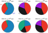Fig. 9

Pie charts of the percentage contributions of the dominant oxygen-bearing molecules to the total elemental oxygen abundance (=3.2 × 10⁻⁴) at r ~ 60 au (T_gas ~ 150 K, inside the water snowline) in the NGC 1333-IRAS 2A envelope model (top three charts) and the NGC 1333-IRAS 4A envelope model (bottom three charts). The left, middle, and right charts show the contributions with L_X = 10²⁸, 10³⁰, and 10³² erg s⁻¹, respectively. The red, dark blue, purple, black, green, and light blue slices are respectively the contributions of CO, H₂O, O, O₂, CO₂, and other molecules (such as CH₃OH).

4.2 Comparison with observations for IRAS 4A

In the left panel of Fig. 10 the observational best-fit $n_{H_{2} O}$ $n_{\mathrm{H}_{2}\mathrm{O}}$ /n_H profile in the IRAS 4A envelope, obtained from van Dishoeck et al. (2021), is overplotted on our model profiles (see also Sect. 3.1 and the top right panel of Fig. 3). This profile is based on analysis of Herschel/HIFI spectra which mainly trace the cold outer part (Mottram et al. 2013; Schmalzl et al. 2014), with the modification of the inner (T_gas > 100 K) water gas abundance from >10⁻⁴ to 3 × 10⁻⁶ (Persson et al. 2012, 2014, 2016). In the cold outer part of the envelope (T_gas < 10² K, r > 10² au) the best-fit profile is consistent with our model profiles for L_X ≲ 10²⁸ erg s⁻¹. In contrast, in the inner warm envelopes (T_gas ≳ 150 K, r ≲ 60 au), the gaseous water abundance in the best-fit profile is 3 × 10⁻⁶ (Persson et al. 2016), which suggests the possibility of efficient X-ray-induced water destructions of gas-phase water molecules with L_X ≳ 10³⁰ erg s⁻¹ in these regions. The reason for this discrepancy between the inner and outer envelope is not clear.

In the cold outer part of the envelope, X-ray-induced photodesorption of water molecules controls the water gas abundance. Therefore, if the rates of X-ray-induced photodesorption of water are much lower (e.g., Y_des(H₂O) ≲ 10⁻⁵ molecules photon⁻¹) than our adopted values, the water gas abundance profiles in the cold outer part of the envelope for L_X ≳ 10³⁰ erg s⁻¹ are expected to be more similar to the observational profile. In Sect. 4.3, we discuss the rates of X-ray-induced photodesorption in detail by conducting additional model calculations.

The 3σ upper limit O₂ gas abundance with respect to H₂ obtained by Yıldız et al. (2013) is ≤ 6 × 10⁻⁹ toward the entire envelope of IRAS 4A using Herschel/HIFI. They estimated that the observed O₂ gas abundance cannot be more than 10⁻⁶ for the inner warm region (r ≲ 10² au). In the right hand panel of Fig. 10, the three model abundance profiles calculated in Yıldız et al. (2013) are overplotted on our model profiles (see also Sect. 3.2 and the top right panel of Fig. 5). The black solid line shows the drop gaseous O₂ abundance profile obtained using the best-fit CO abundance profile produced from the observed C¹⁸O line emission (Yıldız et al. 2012) and assuming O₂ has the same snowline position as CO (i.e., a constant O₂/CO abundance ratio). The blue dashed and the green dotted lines show the gaseous O₂ abundance profiles via their gas-grain modeling with different pre-collapse lifetimes of t_pre = 8 × 10⁵ yr and t_pre = 10⁶ yr, respectively. As the basis for their gas-grain chemical network (Yıldız et al. 2013), the Ohio State University (OSU) gas-grain network Garrod et al. (2008) is used, which also included gas phase reactions, grain surface reactions, and thermal and non-thermal gas-grain interactions. Although the X-ray-induced reactions were not contained, the cosmic-ray-induced reactions were included in their calculations.

These three model profiles are consistent with the above observational upper limit in Yıldız et al. (2013) (the peak temperatures of the models and the observation are similar), and within the values of our chemical modeling at r ≳ 10³ au. At r ~ 10²−6 × 10² au, the gaseous O₂ abundance limit in the drop model is 10⁻⁷, which is similar to the values in our model profiles for L_X ≲ 10³⁰ erg s⁻¹ within one order of magnitude. In contrast, at r < 6 × 10² au, the gaseous O₂ abundance in their gas-grain modeling are much lower (≫10⁻¹⁰) than that in our model profiles and that in the drop model.

We note that L_X of IRAS 4A is thought to be ≳ 10³⁰ erg s⁻¹ by comparing the results of our model calculations and the observationally estimated inner water gas abundances toward IRAS 4A (see discussions above). Thus, on the basis of the discussions about H₂O and O₂ in this subsection, L_X of IRAS 4A is suggested to be around 10³⁰ erg s⁻¹, although thediscrepancy of suggested L_X between the inner and outer envelope discussed above remains (see also Sect. 4.3). Since probing the O and CO₂ gas abundances in the inner envelopes is also difficult (see Sects. 4.1 and 4.5, and Appendix C), observationally obtaining the abundance profiles of other tracers, especially HCO⁺ and CH₃OH, is important to investigate the effects of X-ray-induced chemistry and confine the values of L_X (see Sect. 4.6).

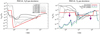Fig. 10

Comparison of our model and observation-based radial profiles for H₂O and O₂ gas fractional abundances in the IRAS 4A envelopes. Left panel: gray-scale plots (from white to black) are the radial profiles of water gas fractional abundances $n_{H_{2} O}$ $n_{\mathrm{H}_{2}\mathrm{O}}$ /n_H in the NGC 1333-IRAS 4A envelope model, which are the same as the color plots in the top right panel of Fig. 3. The red solid line shows the observational best-fit $n_{H_{2} O}$ $n_{\mathrm{H}_{2}\mathrm{O}}$ /n_H profile in the IRAS 4A envelope, obtained from van Dishoeck et al. (2021). This profile is based on analysis of Herschel/HIFI spectra which mainly trace the cold outer part (Mottram et al. 2013; Schmalzl et al. 2014), with the modification of the inner (T_gas > 100 K) water gasabundance from >10⁻⁴ to 3 × 10⁻⁶ (Persson et al. 2016). Right panel: Gray-scale plots (from white to black) are the radial profiles of molecular oxygen gas fractional abundances $n_{O_{2}}$ $n_{\mathrm{O}_{2}}$ /n_H in the NGC 1333-IRAS 4A envelope model, which are the same as the color plots in the top right panel of Fig. 5. The model abundance profiles obtained in Yıldız et al. (2013) are over-plotted. The red solid line shows the drop gaseous O₂ abundance profile by using the C¹⁸O modeling (Yıldız et al. 2012) and assuming O₂ follows the same freeze-out and sublimation processes as C¹⁸O. The blue dashed and the green dotted lines show the gaseous O₂ abundance profiles via their gas-grain modeling with t_pre = 8 × 10⁵ yr and t_pre = 10⁶ yr, respectively. The purple arrows are to indicate that Yıldız et al. (2013) only obtained the upper limit O₂ gas abundance for this object.

4.3 Rates of X-ray-induced photodesorption

In our standard model calculations, we do not include the photodesorption by UV photons generated internally via the interaction of secondary electrons produced by X-rays with H₂ molecules, although we include X-ray-induced photodissociation on dust grains (see also Sects. 2.2.2 and 2.2.3). Our adopted rates of X-ray-induced photodesorption are an approximation based on the UV photodesorption rates (see also Sect. 2.2.2), since experimental constraints for X-ray-induced photodesorption are limited (e.g., Walsh et al. 2014a). Recently, Dupuy et al. (2018) experimentally investigated X-ray-induced photodesorption rates of H₂O, O₂, and other related molecules. According to their experiments, photodesorption yields of H₂O and O₂ at 0.55 keV for a compact amorphous solid water ice at 15 K are 3.4 × 10⁻³ and 4.0 × 10⁻⁴ molecules photon⁻¹. The differences between these values and our adopted values are within a factor of a few (see Table 1).

In addition, Dupuy et al. (2018) simply extrapolated X-ray photodesorption yields for higher X-ray photon energies using the absorption cross sections of water gas. They estimated that the yields of H₂O at 15 K would be ≲10⁻⁴ at >3 keV, although further experimental studies will be needed to obtain accurate values. If we estimate the local average X-ray-induced photodesorption yields (by multiplying the energy-dependent photodesorption yields by the local X-ray spectrum) on the basis of their simply extrapolated results, the yields would become lower in the outer envelope with larger values of N_H, where softer X-rays are more attenuated.

Here we conduct the two types of additional calculations which focus on the rates of X-ray-induced photodesorption and their effect on the chemistry. In the first additional model (see Figs. G.1 and G.2), we include the photodesorption by UV photons generated internally via the interaction of secondary electrons produced by X-rays with H₂ molecules. We scale the cosmic-ray-induced photon flux (10⁴ photons cm⁻² s⁻¹, Walsh et al. 2014a) by the total ionization rate (cosmic rays plus X-rays) relative to the cosmic-ray ionization rate only, and use the revised value in estimating the photodesorption rates. According to our calculations (see Figs. G.1 and G.2), the effects of additional secondary (indirect) X-ray-induced photodesorption is marginal (the abundances are changed by <1%). The direct photodesorption by X-ray photons is the dominant process in our calculations.

Next, in the second additional model (see Figs. 11 and G.3), we switch off the direct X-ray-induced photodesorption and include the secondary (indirect) X-ray-induced photodesorption only. Through this calculation, we can also investigate the impact when the rates of the direct X-ray-induced photodesorption are much smaller than our originally adopted values. As is seen in Figs. 11 and G.3, the effects of X-ray-induced photodesorption are decreased relative to the previous case. In the case of H₂O, the gas-phase abundances outside the water snowline for L_X ≳ 10³⁰ erg s⁻¹ become around two orders of magnitude smaller than those in our standard model and the first additional model. In addition, in the outer part of the envelope, the observational best-fit profile of H₂O gas is now roughly consistent with the models with L_X ≲ 10³⁰ erg s⁻¹. We note that in cases of our standard model calculations (see Sect. 4.2), the best-fit profile is consistent with model profiles for L_X ≲ 10²⁸ erg s⁻¹ in the outer region, whereas with those for L_X ≳ 10³⁰ erg s⁻¹ in the inner region. Thus, lower rates (e.g., Y_des(H₂O) ≲ 10⁻⁵ molecules photon⁻¹) of direct X-ray-induced photodesorption bring the models more in line with the observed abundance profiles, which calls into question whether the direct X-ray-induced photodesorption rates are overestimated. We note that the OH gas abundances at r ~ 10²–10⁴ au for L_X ≳ 10³⁰ erg s⁻¹ become 1–2 orders of magnitude lower than those in our standard model and the first additional model, since OH is efficiently produced by X-ray-induced photodissociation of H₂O gas and fragmental photodesorption of H₂O ice (see also Sect. 3.4). In addition, O₂ gas abundances at r ~ 10²–10⁴ au for L_X ≳ 10³⁰ erg s⁻¹ are up to ten times lower since O₂ is formed in the gas-phase of O and OH (see Sect. 3.2). For other molecules shown in Fig. G.3, the differences in abundances between the standard model and the second additional model are much smaller than those in H₂O, OH, and O₂.

Future experimental and theoretical studies over a wider X-ray energy range are needed to understand how X-ray-induced photodesorption rates behave as a function of the X-ray energy spectrum. X-ray-induced photodesorption yields are also expected to vary for different ice composition. Basalgète et al. (2021a,b) recently investigated the X-ray-induced photodesorption yields of CH₃OH experimentally, and they estimated that the intact yields for mixed methanol-water ices would be more than around two orders of magnitude smaller than those for pure methanol ices.

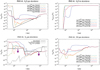Fig. 11

Radial profiles of gaseous fractional abundances of H₂O, O₂, and OH, andicy fractional abundances of H₂O in the NGC 1333-IRAS 4A envelope models. The light green solid lines, the cyan double-dashed dotted lines, and the blue dotted lines show the radial profiles of our standard model calculations, for values of central star X-ray luminosities L_X =10²⁸, 10³⁰, and 10³² erg s⁻¹, respectively (see also Figs. 3, 4, 5, 6). The yellow dashed double-dotted lines, the scarlet dashed dotted lines, and the brown dashed lines show the radial profiles of our additional model calculations for L_X = 10²⁸, 10³⁰, and 10³² erg s⁻¹, respectively. In the additional model calculations, we include the photodesorption by UV photons generated internally via the interaction of secondary electrons produced by X-rays with H₂ molecules (the secondary (indirect) X-ray-induced photodesorption, see Figs. G.1and G.2), and we also switch off the direct X-ray-induced photodesorption (see also Fig. G.3). In the top left panel, the observational best-fit H₂O gas abundance profile obtained in van Dishoeck et al. (2021) is overplotted with the black solid line (see also Fig. 10). In the bottom left panel, the three model O₂ gas abundance profiles obtained in Yıldız et al. (2013) are overplotted (see also Fig. 10).

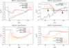Fig. 12

Radial profiles of gaseous fractional abundances of H₂O, O₂, O, and OH in NGC 1333-IRAS 4A envelope models. The yellow solid lines and scarlet dash-dotted lines show the radial profiles of our standard model calculations for values of central star X-ray luminosities L_X = 10²⁸ and 10³² erg s⁻¹, respectively (see also Figs. 3, 5, and 6). The orange dashed double-dotted lines and red dotted lines show those of our test calculations assuming that the product of H₂O photodissociation is 100% atomic oxygen, unlike our standard model (100% OH) (see also Fig. H.1). The orange double-dashed dotted lines and brown dashed lines show those of our test calculations assuming the smaller E_des (j) for atomic oxygen (=800 K) than that in our fiducial model (=1660 K) (see also Fig. H.2). In the top left panel, the observational best-fit H₂O gas abundance profile obtained in van Dishoeck et al. (2021) is overplotted with the black solid line (see also Fig. 10). In the top right panel the three model O₂ gas abundance profiles obtained in Yıldız et al. (2013) are overplotted (see also Fig. 10).

4.4 Model assumptions for chemistry

In our adopted chemical reaction network (see Sect. 2), the X-ray-induced and cosmic-ray-induced photodissociation of H₂O in both gas and ice is the following (McElroy et al. 2013): $H_{2} O + h ν \to OH + H .$ $\begin{equation*}\mathrm{H}_{2}\mathrm{O}+h\nu\rightarrow\mathrm{OH}+\mathrm{H}. \end{equation*}$ (14)

According to van Harrevelt & van Hemert (2008) and Heays et al. (2017), however, there is another route of photodissociation of H₂O: $H_{2} O + h ν \to O + H_{2} / 2 H .$ $\begin{equation*}\mathrm{H}_{2}\mathrm{O}+h\nu\rightarrow\mathrm{O}+\mathrm{H}_{2}/2\mathrm{H}. \end{equation*}$ (15)

Heays et al. (2017) calculated the photodissociation branching ratio of H₂O using various radiation fields as OH/O ~ 3, although it depends on wavelength.

In order to investigate the impacts of this photodissociation branching ratio on the abundances of H₂O and related molecules, in Figs. 12 and H.1 (see Appendix H) we show the gas-phase abundance profiles of H₂O, O₂, O, and OH, which are calculated assuming the extreme case that the product of H₂O photodissociation is 100% atomic oxygen (only Reaction (15) in the gas and the ice), and compare them with the profiles in our standard models (see also Figs. 3, 5, and 6). Since the photodissociation of H₂O is important just inside the snowline (see Sect. 3.1), the abundances around r ≈ 10² au are mainly affected. The OH gas abundances become smaller by a factor of a few at r ≲ 10² au than those in our standard model. For L_X ≲ 10³⁰ erg s⁻¹, the O and O₂ gas abundances increase by around 1–2 orders of magnitude at r ≲ 10² au compared with those in our standard model. For L_X ≳ 10³¹ erg s⁻¹, where O and O₂ gas become dominant oxygen carries, these abundances are similar between these different models. Outside the water snowline r > 10² au, these abundances are almost unchanged.

Except atomic oxygen, the differences of binding energies E_des(j) for dominant molecules between our adopted values and those in recent other chemical modeling are up to around several tens of percent (see Table 2 and e.g., Cuppen et al. 2017; Penteado et al. 2017). In our adopted chemical model, E_des(O) is assumed to be 1660 K, on the basis of recent experimental measurements (He et al. 2014; He & Vidali 2014). Taquet et al. (2016b) and Eistrup & Walsh (2019) adopted similar value of E_des(O). However, some of other recent chemical models (e.g., Eistrup et al. 2016; Bosman et al. 2018b) adopted the older estimated value of 800 K, which is around two times smaller than our adopted values. This value of 800 K has been widely used in many chemical models (e.g., Tielens & Hagen 1982; Hasegawa et al. 1992; Garrod & Pauly 2011), but He et al. (2014) pointed out that it has no strong theoretical derivation and no experimental confirmation.

In order to investigate the impacts of different binding energies of O on molecular abundances, in Figs. 12 and H.2 (see Appendix H) we show the gas-phase abundance profiles of H₂O, O₂, O, and OH, which are obtained from our test calculations assuming the lower E_des(O) (= 800 K) than that in our fiducial model (=1660 K), and compare them with the profiles in our standard models (see also Figs. 3, 5, and 6). The O gas abundances increase by up to one order of magnitude at r ~ (1 − 4) × 10² au than those in our standard model. In contrast, only for L_X ≲ 10²⁸ erg s⁻¹ the O₂ gas abundances decrease by factor of a few at r ~ (1 − 4) × 10² au than those in our standard model. The OH and H₂O gas abundances are similar to those in our standard model.

4.5 H₂O, O₂, and O line observations for other protostars

On the basis of previous PdBI (NOEMA) and Herschel/HIFI observations (Persson et al. 2012, 2014, 2016; Visser et al. 2013), the water gas abundance is around 10⁻⁴ in the inner warm envelope and disk of IRAS 2A. In contrast, the water gas abundances in the inner envelopes and disks of IRAS 4A and 4B are lower by 1–3 orders of magnitude. Through recent ALMA observations, Jensen et al. (2019) estimated that the H₂ ¹⁸ O column densities in the warm inner envelopes around three isolated low-mass Class 0 protostars (L483, B335 and BHR71-IRS1) are a few × 10¹⁵ cm⁻², which is similar to that of IRAS 4B, and around ten times smaller than that of IRAS 2A (Persson et al. 2014). Compared with the results of our chemical modeling, the observational results of IRAS 2A are consistent with the profiles with L_X ≲ 10²⁹ erg s⁻¹. In contrast, the reported inner water gas abundances for IRAS 4A, IRAS 4B, and other objects (~ 10¹–10³ times lower than that for IRAS 2A) are close to the values of our chemical modeling with L_X ≳ 10³⁰–10³¹ erg s⁻¹. Thus, X-ray-induced destruction processes can explain the lower water abundances in the inner envelopes of these objects.

Harsono et al. (2020) show that water vapor is not abundant in the warm envelopes and disks around Class I protostars, and upper limit values of the water gas abundance averaged over the inner warm disk with T_gas > 100 K are ~ 10⁻⁷–10⁻⁵. These lower water gas abundances might also be caused by efficient water gas destruction through X-ray-induced chemistry, in addition to locking up water in icy dust grains. Future detailed water line observations, for example using ALMA for more Class 0 and I objects with various X-ray luminosities, and chemical modeling with detailed physical structure models (e.g., disk+envelope, see also van Dishoeck et al. 2014, 2021; Furuya et al. 2017) will clarify the effects of X-ray-induced chemistry on water and other related molecules, and the water trail from protostellar envelopes to planet-forming regions in disks.

In low-mass protostar observations, only an upper limit and a tentative detection are reported for O₂ lines. This is partly because O₂ does not possess electric dipole-allowed rotational transition lines, and it possess only magnetic-allowed lines (Crownover et al. 1990). In addition to the report of an upper limit toward IRAS 4A using Herschel/HIFI (Yıldız et al. 2013)(see Sects. 1 and 4.2 of this paper), Taquet et al. (2018) recently performed a deep search for the ¹⁶O¹⁸O 234 GHz 2₁ − 0₁ line (E_up = 11.2 K) toward the inner envelope around a low-mass protostar IRAS 16293-2422 B with ALMA, and reported a residual emission at a 3σ level after subtraction of the contaminated two brighter transitions at ± 1 km s⁻¹. However, they considered the detection as tentative, since there is a velocity offset of 0.3–0.5 km s⁻¹ relative to the source velocity. Assuming that the ¹⁶O¹⁸O was not detected and using CH₃OH as a reference species, Taquet et al. (2018) obtained a [O₂]/[CH₃OH] abundance ratio <2–5, which is 3–4times lower than that in comet 67P/Churyumov-Gerasimenko.

The strong far-infrared [O I] lines (such as the ³P₁-³P₂ 63.2 μm line) have been used as outflow and jet tracers in low-mass protostars (e.g., Karska et al. 2013; Nisini et al. 2015; Kristensen et al. 2017), but the inner regions in the protostellar envelopes cannot be probed using these lines because of high dust opacities at far-infrared wavelengths. Spectrally resolved [O I] lines profiles, which can be obtained using instruments such as SOFIA/GREAT, can probe the atomic oxygen abundances in the outer envelopes if the outflow can be properly disentangled (see also discussions in van Dishoeck et al. 2021).

4.6 HCO⁺, CH₃OH, and other molecular line observations

On the basis of our chemical modeling for L_X ≳ 10³⁰–10³¹ erg s⁻¹, HCO⁺ is not efficiently destroyed within the water snowline, and its abundances remain ≳ 10⁻⁹ both inside and just outside the water snowline (see Sect. 3.3). In addition, CH₃OH is not thought to be an efficient tracer of the warm inner envelope and the water snowline position for L_X ≳ 10³⁰–10³¹ erg s⁻¹ (see Sect. 3.5). In these cases, the CH₃OH gas abundances are expected to be much lower (below 10⁻¹⁶) than those with L_X ≲ 10²⁹–10³⁰ erg s⁻¹ (~ 10⁻⁷–10⁻⁶). Thus, observationally obtaining the abundance profiles of HCO⁺ (including its isotopologue H¹³CO⁺) and CH₃OH is important to investigate the effects of X-ray-induced chemistry in protostellar envelopes.

van ’t Hoff et al. (2018a) observationally reported an increase in H¹³CO⁺ emission just outside the water snowline in the IRAS 2A envelope. It is consistent with the profiles of our modeling with L_X ≲ 10²⁹ erg s⁻¹ (see also Sect. 3.3). We note that observationally obtained inner water gas abundances are also consistent with our model profiles for L_X ≲ 10²⁹ erg s⁻¹ (see Sect. 4.5).

van ’t Hoff et al. (2018b) and Lee et al. (2019) reported spatially resolved line images of CH₃OH and other COMs (complex organic molecules) with ALMA toward the disk around the embedded protostar V883 Ori, which is a well-known FU Orionis star (e.g., Cieza et al. 2016). They discussed that the radial extent of CH₃OH gas is around 100 au. In the FU Orionis type stars, sudden increases in the luminosity of the central star will quickly expand the snowline positions to larger radii, which provide good opportunities to study the abundances of COMs in the planet-forming materials (Lee et al. 2019).

Lee et al. (2020) obtained spatially resolved images of CH₃OH and H¹³CO⁺ emission lines with ALMA toward the embedded protostar EC53, in which quasi-periodic emission was reported by the near-infrared monitoring observations (Hodapp et al. 2012) and the submillimeter James Clerk Maxwell Telescope (JCMT) monitoring survey (Herczeg et al. 2017; Yoo et al. 2017), which strongly suggests variable accretion rates. Its luminosities L_bol of 1.7–4.8 L_⊙ (e.g., Evans et al. 2009) and envelope mass M_env of 0.86–1.25 (Lee et al. 2020) are similar to those in IRAS 2A and IRAS 4A (the differences are within a factor of 4–5 times). This source is classified as Class I (Giardino et al. 2007), and L_X is around 1−3 × 10³⁰ erg s⁻¹, according to XMM-Newton X-ray observations (Preibisch 2003) and Chandra X-ray observations (Giardino et al. 2007). In this observation, the H¹³CO⁺ line emission is depleted near the continuum peak, where the CH₃OH line emission is present. The CH₃OH emission is more extended than the expected water snowline from the current luminosity of the central star, indicating previous outburst events. However, the derived CH₃OH gas abundance for EC 53 is two orders of magnitude lower than the CH₃OH abundance of ~10⁻⁸ for V883 Ori (Lee et al. 2019), despite the similar size of the methanol emitting region. Comparing with the profiles of our modeling, those observed profiles of H¹³CO⁺ and CH₃OH abundances for EC 53 can be explained if L_X is around × 10²⁹–10³⁰ erg s⁻¹, which is roughly consistent with the observed values of L_X.

Hsieh et al. (2019) reported the detections of the HCO⁺ (3–2) line with ALMA toward the envelopes around 18 Class 0 and 11 Class I protostars in the Perseus molecular cloud, and also the detections of the CH₃OH 254.015 GHz (2_0,2 − 1_−1,1) line toward six of the above sources in which the HCO⁺ line was detected. They discussed the four sources where the CH₃OH line was detected, and found that the measured HCO⁺ peak radii broadly agreed with the CH₃OH emission extents, except two Class 0 sources with very weak CH₃OH emission. In these two Class 0 objects (L1455-IRS4 and L1448-IRS2), both HCO⁺ and CH₃OH emissions have a similar peak position at the center. Our modeling would suggest that these two sources have strong X-ray emission, destroying H₂O and CH₃OH in the inner regions, leading to weak CH₃OH and strong HCO⁺ emission, while in the other sources the X-ray luminosities would be lower. This can be tested by independent determination of the X-ray luminosities for these sources, although observations of X-ray luminosities toward embedded Class 0 protostars are difficult (see Sect. 2.1.2).

CH₃OH and C₂H are the representative products of hot corino chemistry and warm carbon chain chemistry (WCCC) in star-forming cores, respectively (e.g., Sakai & Yamamoto 2013; Imai et al. 2016; Oya et al. 2016; Higuchi et al. 2018; Aikawa et al. 2020; Yang et al. 2021). As shown in Figs. 7 and D.1, the dependence of radial profiles of C₂H gas fractional abundances on X-ray fluxes are much smaller than those of CH₃OH gas fractional abundances, in the inner envelopes (r ≲ 300 au). As the X-ray flux increases, the CH₃OH gas fractional abundances significantly decrease (from 10⁻⁷–10⁻⁶ to < 10⁻¹⁵) at r ≲ 300 au, whereas the C₂H gas fractional abundances change within two orders of magnitude. Aikawa et al. (2020) investigated the physical conditions that affect the hot corino chemistry and WCCC, and described that the deficiency of COMs (including CH₃OH) in prototypical WCCC sources is hard to reproduce within their models. They discussed that the gas-phase destruction processes of CH₃OH and other COMs within several 10⁴ yr after sublimation from dust grains would be important (Charnley et al. 1992; Nomura et al. 2009; Taquet et al. 2016a). X-ray-induced destruction reactions discussed in this paper would help to destroy these molecules within the above timescale.

Recently, the line observations of CH₃OH and other molecules (including COMs and C₂H) with much higher spatial resolutions (Δr ≲ several tens of au) have been conducted with ALMA and VLA toward disks and inner envelopes around Class 0 and I protostars (e.g., Sahu et al. 2019; Bianchi et al. 2020; De Simone et al. 2020, and FAUST⁷). These detailed observations can also be used to constrain the effects of X-ray-induced chemistry on the abundance profiles of HCO⁺, CH₃OH, and other molecules. In addition, future molecular line observations (e.g., ngVLA⁸) will also be helpful. They are expected to constrain the inner gas abundances of CH₃OH, other COMs (Öberg et al. 2018), HCO⁺, and NH₃, which are also affected by X-ray-induced chemistry (see Appendix E and Zhang et al. 2018), creating a more complete picture of the oxygen chemistry and opening a window into the independent nitrogen chemistry. Moreover, since the dust opacities in the frequencies of ngVLA are smaller than those of ALMA (also see, e.g., De Simone et al. 2020), these observations will be useful to trace the inner gas abundances more precisely.

Particles are accelerated in shocks along the protostellar jets and on the protostellar surfaces, and they can enhance the cosmic-ray ionization rates in protostellar envelopes (e.g., Padovani et al. 2016). However, because of the differences in energies, they are much more transparent compared with X-rays, and they affect the ionization rates and thus the abundances of ion molecules (such as HCO⁺ and N₂H⁺) not only in the inner regions, but also in the outermost regions, such as r > 10³ au (Ceccarelli et al. 2014; Favre et al. 2017). Ceccarelli et al. (2014) reported a HCO⁺/N₂H⁺ abundance ratio of approximately 3–4 in the outer envelopes (r > a few × 10³ au) around the protostar OMC-2 FIR4 from Herschel observations, which was very low compared to that in other protostellar envelopes (≫ 10). They suggested that the cosmic-ray ionization rate is around 10⁻¹⁴ s⁻¹, which is much higher than the average value in dense clouds (~ 10⁻¹⁷ s⁻¹, Umebayashi & Nakano 2009).

In addition, van ’t Hoff et al. (2018a) conducted a first-order approximation of the effect of cosmic-ray ionization rates on the HCO⁺ gas abundances in the outer envelopes by considering the main formation (CO+H $_{3}^{+}$ $_{3}^{+}$ ) and destruction (HCO⁺ + e⁻) reactions of HCO⁺ outside the water snowline. Assuming a steady state and similar abundances for HCO⁺ and electron ( $n_{{HCO}^{+}} / n_{H} \approx$ $n_{\mathrm{HCO}^{+}}/n_{\mathrm{H}}\,{\approx}\,$ $n_{e^{-}} / n_{H}$ $n_{\mathrm{e}^{-}}/n_{\mathrm{H}}$ ), they obtained the following expression for the HCO⁺ gas densities $n_{{HCO}^{+}}$ $n_{\mathrm{HCO}^{+}}$ in the outer envelopes, 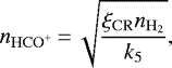$n_{{HCO}^{+}} = \sqrt{\frac{ξ_{CR} n_{H_{2}}}{k_{5}}},$ $\begin{equation*} n_{\mathrm{HCO}^{+}}\,{=}\,\sqrt{\frac{\xi_{\mathrm{CR}}n_{\mathrm{H}_{2}}}{k_{5}}}, \end{equation*}$ (16)

where k₅ is the rate coefficient of the main destruction reaction of HCO⁺ + e⁻ (for more details, see Appendix B of van ’t Hoff et al. 2018a). Thus, with investigating the abundances of ion molecules such as HCO⁺ both the inner and outer regions, we could distinguish the effects of X-ray-induced ionization and cosmic-ray-induced ionization accelerated by protostellar jets, for example. According to our model calculations (ξ_CR(r) = 10⁻¹⁷ s⁻¹), the HCO⁺ abundances at r ≳ 10³ au are ~ 10⁻⁹–10⁻⁸ for IRAS 2A, and ~ 10⁻¹⁰–10⁻⁹ for IRAS 4A. Thus, if the HCO⁺ abundances at these radii are more than an order of magnitude higher, ξ_CR(r) is estimated to be ≳ 10⁻¹⁵ s⁻¹.

We note that Bruderer et al. (2009) and Benz et al. (2016) offered an alternative explanation for enhanced HCO⁺, originating in the UV irradiated warm outflow cavity walls. Spatially resolved observations for HCO⁺ lines are needed to distinguish the scenarios.

4.7 Chemical evolution from envelopes to disks

In our chemical modeling we assume that the physical structures (especially the radial $n_{H_{2}}$ $n_{\mathrm{H}_{2}}$ and T_gas profiles) are constant throughout 10⁵ yr. However, the timescale of the main accretion phase of protostars (Class 0-I) is around a few 10⁵ yr (Dunham et al. 2014; Kristensen & Dunham 2018), and material in the envelopes moves inward (e.g., Visser et al. 2009, 2011; Harsono et al. 2015; Furuya et al. 2017). According to our calculations, for the highest X-ray luminosities of L_X ≳ 10³¹ erg s⁻¹, the X-ray-induced reactions in the inner envelopes proceed with shorter timescales of t < 10³ yr than the timescale of the main accretion phase, although the timescale of grain surface chemistry are longer (t ≫ 10⁵ yr, see also Yoneda et al. 2016). Aikawa et al. (2008, 2020) suggested that the infalling material passes through the region with T_gas ~ 10¹–10² K in several 10⁴ yr, and fall into the central star and the disk ~10² yr after they enter the region with T_gas > 10² K. Therefore, the molecular abundances in the inner envelopes, especially in the innermost region, would be affected because of such inward accretion, unless they enter a rotating disk-like structure (Schöier et al. 2002).

In our chemical modeling of this paper, we assume that X-ray luminosities are constant throughout 10⁵ yr. However, X-ray luminosities of central protostars and X-ray fluxes in surrounding envelopes are expected to change over time because protostar X-ray flares are the dominant X-ray source, and they occur repeatedly every 10 days (Takasao et al. 2019). In the presence of strong X-ray fluxes, water is considered to be efficiently destroyed on a very short timescale of t < 10³ yr (Stäuber et al. 2006) in the disks and the inner envelopes around protostars. Thus, repetition of sudden increase (and decrease) of X-ray luminosities would also affect molecular abundances in the disks and inner envelopes around Class 0 and I protostars.

Detailed chemical modeling with time-dependent physical structures of disks and envelopes around Class 0 and I protostars will be important in the future to understand the effects of X-ray-induced chemistry on the abundance profiles of water and related molecules in detail. We note that Cleeves et al. (2017) reported the time variation of the H¹³CO⁺ J = 3−2 line intensities in a Class II disk between three observational epochs, and they discussed that the enhancement of HCO⁺ abundance in the upper layer of the disk would be explained by X-ray driven chemistry during large X-ray flare events.Waggoner & Cleeves (2019) discussed that the day-scale impulsive increase and decrease in the H₂O gas abundances in the surfaces of Class II disks could be caused by the time dependent chemistry driven by X-ray flares.

According to our chemical modeling, X-ray-induced chemistry affects the abundances profiles of H₂O and other dominant molecules, such as O, O₂, HCO⁺, CH₃OH, OH, CO₂, CH₄, HCN, and NH₃. In the presence of strong X-ray fields (with L_X ≳ 10³⁰–10³¹ erg s⁻¹), the abundances of H₂O, CH₃OH, CH₄, HCN, and NH₃ significantly decrease in the inner envelopes around protostars, and CO, O₂, O become the dominant oxygen carriers. In addition, on the basis of Figs. C.1– E.1, CO and N₂ become the dominant carbon and nitrogen carries under such strong X-ray fields. We note that the material in the protostellar envelopes accretes into disks, thus the molecular abundances in protostellar envelopes determine the initial abundances of chemical evolution in disks, where planet formation occurs (see also the recent review by Öberg & Bergin 2021). In many studies of chemical modeling in disks (e.g., Walsh et al. 2015; Bosman et al. 2018b), initial chemical abundances were assumed to be inherited from dark clouds, pre-stellar cores, and protostellar envelopes, and they are water rich, on the basis of previous observations (e.g., Visser et al. 2009, 2011; Boogert et al. 2015). However, whether the disk chemical evolution is started from initial abundance conditions of the chemical reset (by e.g., irradiation, accretion shocks) or the inheritance from the dark clouds and protostellar envelopes is an important question (e.g., Yoneda et al. 2016; Coutens et al. 2020; Jørgensen et al. 2020; van’t Hoff et al. 2020; Öberg & Bergin 2021). Eistrup et al. (2016, 2018) and Notsu et al. (2020) discussed that the chemical abundances in Class II disks are strongly affected by ionization rates in disks and the adopted initial molecular abundances (inheritance or reset). In the presence of strong X-ray fields (with L_X ≳ 10³⁰–10³¹ erg s⁻¹), the molecular abundances in protostellar envelopes are also altered from inheritance initial molecular abundances.

In future studies, the chemical modeling in disks with initial abundances which consider the effects of X-ray-induced chemistry discussed in this paper will be important to understand the chemical evolution history in disks and the chemical compositions of exoplanets (e.g., Notsu et al. 2020; Turrini et al. 2021).

5 Conclusions

We investigated the radial dependence of the abundances of water and related molecules on X-rays in Class 0 low-mass protostellar envelopes, and identify potential oxygen carriers other than water. We used a detailed gas-grain chemical reaction network including X-ray-induced chemical processes. Gas-phase reactions, thermal and non-thermal gas-grain interactions,and grain-surface reactions are included in our adopted chemical reaction network. For the physical structures of the Class 0 protostellar envelopes, we adopted two types of spherically symmetric radial gas temperature T_gas and molecular hydrogen number density $n_{H_{2}}$ $n_{\mathrm{H}_{2}}$ profiles for IRAS 2A and IRAS 4A in order to examine the effect of density differences on X-ray-induced chemistry. Our findings can be summarized as follows:

Outside the water snowline (T_gas < 10² K, r > 10² au), if X-ray luminosities of the central protostars L_X are larger than 10³⁰ erg s⁻¹, water gas fractional abundances are increased (up to $n_{H_{2} O}$ $n_{\mathrm{H}_{2}\mathrm{O}}$ /n_H ~ 10⁻⁸–10⁻⁷) compared with the values ( $n_{H_{2} O}$ $n_{\mathrm{H}_{2}\mathrm{O}}$ /n_H ~ 10⁻¹⁰) for L_X < 10³⁰ erg s⁻¹. In addition, water ice abundances are around 2 × 10⁻⁴ outside the water snowline for L_X ≲ 10³⁰ erg s⁻¹, and they become much lower (below to $n_{H_{2} O, ice}$ $n_{\mathrm{H}_{2}\mathrm{O}, \mathrm{ice}}$ /n_H ~ 10⁻⁸ at a few ×10² au) for L_X ≳ 10³¹ erg s⁻¹. X-ray-induced photodesorption of water ice affects this region. Since there are limited experimental constraints for X-ray-induced photodesorption rates, future theoretical and experimental studies for the X-ray-induced photodesorption over wider X-ray energy ranges are important.
Inside the water snowline (T_gas > 10² K, r < 10² au), for L_X ≲ 10²⁹–10³⁰ erg s⁻¹, water maintains a high abundance of ~10⁻⁴, and water and CO are the dominant oxygen carriers. For L_X ≳ 10³⁰–10³¹ erg s⁻¹, the water gas abundances significantly decrease just inside the water snowline (T_gas ~ 100–250 K, down to $n_{H_{2} O}$ $n_{\mathrm{H}_{2}\mathrm{O}}$ /n_H ~ 10⁻⁸–10⁻⁷) and in the innermost regions (T_gas ~ 250 K, $n_{H_{2} O}$ $n_{\mathrm{H}_{2}\mathrm{O}}$ /n_H ~ 10⁻⁶). In the presence of strong X-ray fields, gas-phase water is mainly destroyed with the ion-molecule reactions and the X-ray-induced photodissociation. In our chemical modeling, the former ion-molecule reactions are dominant processes for the water gas destruction inside the water snowline. For L_X ≳ 10²⁹–10³⁰ erg s⁻¹, the X-ray ionization rates ξ_X(r) are larger than our adopted cosmic ray ionization rate ξ_CR(r)(= 1.0 × 10⁻¹⁷ s⁻¹) within the water snowline. In the innermost hot region water abundances become relatively high since the two-body water formation reaction (OH+H₂) becomes efficient.
As the X-ray fluxes become larger, the O₂ and O gas abundances become larger both inside and outside the water snowline. Inside the water snowline, the O₂ and O gas abundances are both much smaller (<10⁻⁸) for L_X ≲ 10²⁸–10²⁹ erg s⁻¹. In contrast, for L_X ≳ 10²⁹–10³⁰ erg s⁻¹, their abundances become larger, and reach about 10⁻⁴ with L_X ≳ 10³¹ erg s⁻¹. Compared with the water gas abundances, both O₂ and O gas abundances have opposite dependence on X-ray fluxes. For L_X ≳ 10³⁰–10³¹ erg s⁻¹, O₂, O, and CO become the dominant oxygen carriers in the inner envelopes (r ≲ a few ×10² au).
According to previous studies, the most abundant destroyer of HCO⁺ in warm gas is water, and the radius of the CH₃OH snowline (~2 × 10² au) is around two times larger than that of the water snowline (~10² au). Thus, CH₃OH and HCO⁺ (and alsoH¹³CO⁺) gas lines have been used as good tracers of the water snowline. In our modeling, the HCO⁺ and CH₃OH gas abundances respectively increase and decrease within the water snowline as the X-ray fluxes become larger. For L_X ≳ 10³⁰–10³¹ erg s⁻¹, the HCO⁺ abundances within the water snowline increase by four orders of magnitude, and reach more than 10⁻⁹–10⁻¹⁰, which are similar to those outside the water snowline. In contrast, CH₃OH gas abundance in these radii decrease from ~10⁻⁷–10⁻⁶ to <10⁻¹⁶. Therefore, both HCO⁺ and CH₃OH cannot be used as tracers of the water snowline position for L_X ≳ 10³⁰–10³¹ erg s⁻¹. Observationally obtaining the abundance profiles of HCO⁺, H¹³CO⁺, and CH₃OH is important to investigate the effects of X-ray-induced chemistry in protostellar envelopes.
The gas-phase fractional abundances of OH and CO₂ increase in the outer envelope as the X-ray fluxes become larger. At r < a few hundred au, for L_X ≲ 10²⁹–10³⁰ erg s⁻¹, OH and CO₂ gas abundances increase as the X-ray fluxes become larger. CO₂ gas abundances are ~10⁻⁵–10⁻⁴ at L_X ~ 10²⁹–10³⁰ erg s⁻¹. In these cases CO₂ also becomes one of the dominant oxygen-bearing molecules, especially in the regions where the abundances of O₂ gas and H₂O are similar. However, OH and CO₂ gas abundances decrease for L_X ≳ 10³⁰–10³¹ erg s⁻¹, and CO₂ gas abundances are ≲10⁻⁶ at L_X ≳ 10³¹–10³² erg s⁻¹.
As X-ray fluxes become large the fractional abundances of gas-phase CH₄, HCN, and NH₃ decrease within their own snowline positions. The radial CO and N₂ abundance profiles are constant for the various X-ray luminosities, and they are the dominant carbon and nitrogen carriers under the strong X-ray fields.
The effects of X-ray-induced chemistry are greater in the IRAS 2A model than those in the IRAS 4A model, which has 3–6 times higher densities.
Comparing the results of our modeling with the observationally obtained inner gas abundances of H₂O and H¹³CO⁺, L_X of IRAS 2A is estimated to be ≲10²⁹ erg s⁻¹. In addition, our models with L_X ~ 10³⁰ erg s⁻¹ would explain both the low inner water gas abundances and the upper limit values of O₂ gas abundances obtained by previous observations toward IRAS 4A. However, in the cold outer part of the envelope, the best-fit profile obtained from observations toward IRAS 4A is consistent with our model profiles for L_X ≲ 10²⁸ erg s⁻¹. The discrepancy of suggested L_X between the inner and outer envelope remains unless the rates of direct X-ray-induced photodesorption of water are around two orders of magnitude lower than our adopted values. Since probing the O and CO₂ gas abundances in the inner envelopes is difficult, observationally obtaining the abundance profiles of other tracers, especially HCO⁺ and CH₃OH, is important to investigate the effects of X-ray-induced chemistry and confine the values of L_X.

On the basis of our chemical modeling, X-ray-induced chemistry strongly affects the abundances of water and other related molecules (e.g., O₂, O, HCO⁺, CH₃OH, CO₂, OH, CH₄, HCN, and NH₃) especially inthe inner regions, and can explain the observed low water abundances in the inner protostellar envelopes. We find that gas-phase destruction of molecules by X-rays as well as X-ray-induced photodesorption processes are important. Future molecular line observations toward the disks and envelopes around low-mass protostars, for example using ALMA and ngVLA, willconstrain the effects of X-ray-induced chemistry. In addition, it will be important to discuss how the X-ray-induced chemistry at protostar phases affect the initial abundances and chemical evolution in planet-forming disks.

Acknowledgements

We are grateful to Daniel Harsono, Umut A. Yıldız, Joseph C. Mottram, Merel L.R. van’t Hoff, and Lars E. Kristensen for giving us the data of temperature, number density, and water abundance profiles estimated from previous observations of Class 0 protostellar envelopes. We thank Shinsuke Takasao and Masanobu Kunitomo for their important comments about X-ray fields in protostars. We are also grateful to Yuri Aikawa for her useful comments on chemical evolutions and to Nami Sakai for her comments on the possibility of future ngVLA observations. We thank the referee for important suggestions and comments. Our numerical studies were carried out on PC cluster at Center for Computational Astrophysics (CfCA), National Astronomical Observatory of Japan (NAOJ), and on computer systems at Leiden Observatory, Leiden University. S.N. is grateful for support from JSPS (Japan Society for the Promotion of Science) Overseas Research Fellowships, RIKEN Special Postdoctoral Researcher Program (Fellowships), and MEXT/JSPS Grants-in-Aid for Scientific Research (KAKENHI) 20K22376, 20H05845, and 20H05847. C.W. acknowledges financial support from the University of Leeds and from the Science and Technology Facilities Council (grant numbers ST/R000549/1 and ST/T000287/1). H.N. is supported by MEXT/JSPS Grants-in-Aid for Scientific Research (KAKENHI) 18H05441, 19K03910 and 20H00182, NAOJ ALMA Scientific Research grant No. 2018-10B, and FY2019 Leadership Program at NAOJ.

Appendix A Dependance of X-ray-induced chemistry on gas number density

In this section we investigate the dependance of X-ray-induced chemistry on the gas number density. The rates of formation or destruction for gas-phase species Y due to the X-ray-induced photoionization and photodissociation reactions are scaled with ζ_X (r) × n_Y, and these are first-order kinetic processes with regard to gas densities. In contrast, ion-molecule reactions and neutral-neutral reactions are second-order kinetic processes with regard to gas densities. Thus, given the same X-ray ionization rates ζ_X (r) and gas temperatures T_gas, the more important the second-order processes are, the less important the former first-order processes are as the gas density increases.

At r ~ 60 au (inside the water snowline), the gas density in IRAS 4A ( $n_{H_{2}}$ $n_{\mathrm{H}_{2}}$ = 1.1 × 10⁹ cm⁻³) is around 5.5times larger than that in IRAS 2A ( $n_{H_{2}}$ $n_{\mathrm{H}_{2}}$ = 2.0 × 10⁸ cm⁻³), whereas the gas temperatures are similar (T_gas ~ 140 K for IRAS 2Aand ~150 K for IRAS 4A). For L_X = 10³² erg s⁻¹, ζ_X (r) in IRAS 4A (2.0 × 10⁻¹⁴ s⁻¹) is around 4.4 times lower than that in IRAS 2A (8.8 × 10⁻¹⁴ s⁻¹). We conducted a test chemical calculation, in which we adopt the IRAS 4A physical structure ( $n_{H_{2}}$ $n_{\mathrm{H}_{2}}$ and T_gas) at r ~ 60 au and L_X = 10³² erg s⁻¹, and rescale ζ_X(r) to the value at a similar radius in the IRAS 2A model. We compare the rates of reactions of this test calculation with those of the standard IRAS 2A model.

In this test calculation, at t = 10⁵ yr, the fractional abundance and absolute number density of water are 6.9 × 10⁻⁸ and 1.5 × 10² cm⁻³, respectively, and the same for HCO⁺ are 4.2 × 10⁻⁹ and 9.4 cm⁻³, respectively. On the basis of these values the rate coefficient of the ion-molecule reaction with H₂O+HCO⁺ →CO+H₃O⁺, k₆, is ~ 3.5 × 10⁻⁹ cm³ s⁻¹ (Adams et al. 1978), and the reaction rate, R(6) = k₆ $n_{H_{2} O}$ $n_{\mathrm{H}_{2}\mathrm{O}}$ $n_{{HCO}^{+}}$ $n_{\mathrm{HCO}^{+}}$ , is ~ 2.2 × 10⁻⁵ cm⁻³ s⁻¹ at t = 10⁵ yr. In contrast, the rate coefficient of X-ray-induced photodissociation leading to H+OH, k₇, is ~ 8.6 × 10⁻¹¹ s⁻¹ (Gredel et al. 1989), and the reaction rate, R(7) = k₇ $n_{H_{2} O}$ $n_{\mathrm{H}_{2}\mathrm{O}}$ , is ~ 1.3 × 10⁻⁸ cm⁻³ s⁻¹ at t = 10⁵ yr.

Comparing these reaction rates with those of the standard IRAS 2A model (see Sect. 3.1), the differences of the reaction rates are larger in the ion-molecule reaction (R(6)∕R(1) ~ 25) than in the X-ray-induced photodissociation (R(7)∕R(2) ~ 2.5) because the former reaction is the second-order process and the latter reaction is the first-order process. Thus, as the gas densities increase, thesecond-order processes including ion-molecule reactions become much more dominant compared with the first-order processes including X-ray-induced photodissociation.

Appendix B Subgrid calculations for the IRAS 4A envelope models

Figure B.1 shows the radial profiles of H₂O, O₂, O, OH, HCO⁺, and CH₃OH gas fractional abundances in the IRAS 4A envelope models, with X-ray luminosities between L_X = 10³⁰ and 10³¹ erg s⁻¹. We plot these subgrid model profiles since there is a large jump in abundances in this X-ray luminosity range (see Figs. 3–7). For the abundance profiles of H₂O gas, between 10³⁰ and 2 × 10³⁰ erg s⁻¹ seems to be the clear boundary, which decreases from ~10⁻⁴ to <10⁻⁷ at r ≲ 10² au. For the abundance profiles of HCO⁺, OH, and CH₃OH gas, between 10³⁰ and 2 × 10³⁰ erg s⁻¹ also seems to be the clear boundary. In comparison, the abundance profiles of O₂ and O gas gradually increase in the inner region as the values of L_X increase from 10³⁰ to ~ 6 × 10³⁰ erg s⁻¹.

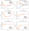Fig. B.1

Radial profiles of gaseous fractional abundances of H₂O, O₂, O, OH, HCO⁺, and CH₃OH in the NGC 1333-IRAS 4A envelope models, with X-ray luminosities between L_X = 10³⁰ and 10³¹ erg s⁻¹. The line color gradually changes from yellow to orange, red, and brown as the value of L_X increases. In the top left panel, the observational best-fit H₂O gas abundance profile obtained in van Dishoeck et al. (2021) is overplotted; in the top right panel, the three model O₂ gas abundance profiles obtained in Yıldız et al. (2013) are overplotted (see Fig. 10).

Appendix C CO₂ and CO fractional abundances

Figure C.1 shows the radial profiles of CO₂ gas and ice fractional abundances $n_{{CO}_{2}}$ $n_{\mathrm{CO}_{2}}$ /n_H in IRAS 2A(left panels) and IRAS 4A (right panels) envelope models, for the various X-ray luminosities. At r ~ 3 × 10²−4 × 10³ au (in the IRAS 2A model) and r ~ 3 × 10²−2 × 10³ au (in the IRAS 4A model), which are the regions between CO₂ and CO snowlines, CO₂ ice abundances are around 10⁻⁶ for L_X ≲ 10³⁰ erg s⁻¹. In contrast, for L_X ≳ 10³¹ erg s⁻¹, CO₂ ice abundances increase (up to 10⁻⁵) in these regions. On the basis of Drozdovskaya et al. (2016), Eistrup et al. (2016, 2018), and Bosman et al. (2018b), in the presence of X-ray fluxes the X-ray-induced photodissociation of H₂O ice forms OH radicals within the ice mantle, which subsequently react with CO on grain surfaces to form CO₂ ice inside the CO snowline.

CO₂ gas abundances at r ≲ 10⁴ au in the IRAS 2A model and at r ≲ 6 × 10³ au in the IRAS 4A model are affected by strong X-ray fluxes. For low and moderate X-ray luminosities⁹, CO₂ gas abundances decrease, and reach ≲ 10⁻⁹ at r ~ 3 × 10²–10³ au (outside the CO₂ snowline). In contrast, for high X-ray luminosities,CO₂ gas abundances increase, and they reach around 10⁻⁶ (for IRAS 2A) and 10⁻⁷ (for IRAS 4A) at these radii for L_X ~ 10³² erg s⁻¹. At r ≲ 3 × 10² au (inside CO₂ snowline), CO₂ abundances are around 10⁻⁶–10⁻⁵ for low X-ray luminosities. In addition, like OH, the CO₂ gas abundances increase as the X-ray fluxes become larger, and they reach ~ 10⁻⁵–10⁻⁴ for moderate X-ray luminosities, However, they decrease for high X-ray luminosities. At L_X ≳ 10³¹ erg s⁻¹ in the IRAS 2A model and L_X ≳ 10³² erg s⁻¹ in the IRAS 4A model, the CO₂ gas abundances are around 3 × 10⁻⁷–10⁻⁶.

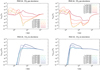Fig. C.1

Radial profiles of CO₂ gas and ice fractional abundances $n_{{CO}_{2}}$ $n_{\mathrm{CO}_{2}}$ /n_H (top panels) and $n_{{CO}_{2}, ice}$ $n_{\mathrm{CO}_{2},\mathrm{ice}}$ /n_H (bottom panels) in NGC 1333-IRAS 2A (left) and NGC 1333-IRAS 4A (right) envelope models.

Outside the CO₂ snowline, CO₂ gas is supplied by X-ray-induced photodesorption reaction of CO₂ ice. In the inner envelope, gas-phase CO₂ is mainly formed by two-body reactions of CO+OH (Bosman et al. 2017), and destroyed via X-ray-induced photodissociation. Therefore, CO₂ abundance profiles strongly depend on the radial profiles of X-ray fluxes and OH abundances.

The CO₂ abundances in the outer envelopes around low-mass protostars can be probed through the observations CO₂ ro-vibrational lines with JWST (see also Sect. 4.1), as done for high-mass protostellar envelopes using ISO (van Dishoeck et al. 1996; Boonman et al. 2003). For low-mass protostellar envelopes, a hint of gas-phase CO₂ lines has been obtained using Spitzer (see, e.g., Poteet et al. 2013). We note that high dust opacities in the near and mid-infrared wavelengths make it difficult to probe theCO₂ gas abundances directly in the inner envelopes around low-mass protostars.

Boonman et al. (2003) and Bosman et al. (2018a) noted the disagreements of CO₂ gas abundances within the CO₂ snowline between models (~10⁻⁵) and observations (~10⁻⁷), both for high-mass protostar envelopes and Class II disks. Bosman et al. (2018a) discussed that the CO₂ should be destroyed within 10⁴ yr after the sublimation of CO₂ ice. X-ray-induced destruction reactions discussed in this paper would help to destroy CO₂ molecules within the above timescale, assuming that CO₂ chemistry is similar among these source types.

Figure C.2 shows the radial profiles of CO gas and ice fractional abundances n_CO/n_H in the IRAS 2A and IRAS 4A envelope models, for the various X-ray luminosities. Unlike other dominant oxygen-bearing molecules (e.g., H₂O, O₂, O, CO₂), CO gas and ice abundances do not depend on X-ray fluxes. The CO gas fractional abundances are around 10⁻⁴ at r ≲ 3 × 10³ au at IRAS 2A and r ≲ 10³ au at IRAS 4A (within the CO snowline), and CO ice fractional abundances are around 10⁻⁴ at r ≳ 4 × 10³ au at IRAS 2A and r ≳ 10³ au at IRAS 4A (outside the CO snowline).

With an ISM level cosmic-ray ionization rate of ξ_CR(r) = 1.0 × 10⁻¹⁷ s⁻¹, longer timescale (>10⁶ yr, the typical age of Class II disks) than that in our modeling (10⁵ yr, the typical age of Class 0 protostars) is required to achieve a CO depletion by a factor of 10 and more (Bosman et al. 2018b; Eistrup et al. 2018; Schwarz et al. 2018). Moreover, in the inner envelopes where ξ_X (r) > ξ_CR(r), efficient X-ray-induced destruction reactions of other dominant molecules, especially H₂O, supply more atomic oxygen, which reacts with C⁺ and returns to CO. According to previous studies of chemical modeling on a timescale of > 10⁶ yr, CO is chemically processed and the carbon is sequestered into less volatile species such as CH₃OH, CH₄, and CO₂ (e.g., Furuya & Aikawa 2014; Yu et al. 2016; Bosman et al. 2018b; Schwarz et al. 2018, 2019; Krijt et al. 2020).

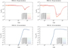Fig. C.2

Radial profiles of CO gas and ice fractional abundances n_CO/n_H (top panels) and n_CO,ice/n_H (bottom panels) in NGC 1333-IRAS 2A (left) and NGC 1333-IRAS 4A (right) envelope models.

According to recent observations (e.g., ALMA), CO gas abundances in the Class 0-I disks with < 10⁶ yr are consistent with the ISM abundance (~10⁻⁴) within a factor of 2 (Harsono et al. 2014; van’t Hoff et al. 2020; Zhang et al. 2020), nearly one order of magnitude higher than the average value in 10⁶–10⁷ yr Class II disks (e.g., Ansdell et al. 2016; Long et al. 2017; Zhang et al. 2019; Bergner et al. 2020).

Appendix D CH₄, HCN, and C₂H fractional abundances

The top panels of Fig. D.1 show the radial profiles of CH₄ gas fractional abundances $n_{{CH}_{4}}$ $n_{\mathrm{CH}_{4}}$ /n_H in the IRAS 2A and IRAS 4A envelope models for the various X-ray luminosities. For L_X ≲ 10²⁸ erg s⁻¹, the CH₄ gas abundances are around (3−8) × 10⁻⁶ at r ≲ 10³ au in the IRAS 2A model and at r ≲ 6 × 10² au in the IRAS 4A model (within the CH₄ snowline). As the X-ray flux becomes larger, the CH₄ gas abundances in these radii decrease. For L_X ≳ 10³¹ erg s⁻¹, the CH₄ gas abundances are around 10⁻⁹–10⁻⁸ at r ≲ 10² au.

The X-ray-induced photodissociation and ion-molecule reactions (e.g., He⁺, H $_{3}^{+}$ $_{3}^{+}$ ) are considered the dominant destruction processes of CH₄ in the inner envelopes (e.g., Aikawa et al. 1999; Eistrup et al. 2016). We note that ion-molecule reactions of gas-phase CH₄ (e.g., with C⁺ within the CH₄ snowline) are important to form unsaturated carbon chain molecules, such as C₂H, C₃H₂, and C₄H (WCCC, e.g., Hassel et al. 2008; Sakai et al. 2008; Sakai & Yamamoto 2013; Aikawa et al. 2012, 2020).

The middle panels of Fig. D.1 show the radial profiles of HCN gas fractional abundances n_HCN/n_H in the IRAS 2A and IRAS 4A envelope models for the various X-ray luminosities. The binding energy of HCN is somewhat smaller than that of H₂O, and is similar to that of CH₃OH (E_des(HCN) = 3610 K, E_des(H₂O) = 4880 K, E_des(CH₃OH) = 3820 K, see Table 2), and the HCN snowline position (~ 2 × 10² au) exists outside the water snowline (~10² au). For low X-ray luminosities, the HCN gas abundances are around ~ 10⁻⁶–10⁻⁵ within the HCN snowline. As the X-ray flux increases, the HCN gas abundances in these radii decrease. For high X-ray luminosities, the HCN gas abundances are ≲ 10⁻⁹ within the HCN snowline. The X-ray-induced photodissociation and ion-molecule reactions (e.g., with He⁺, H $_{3}^{+}$ $_{3}^{+}$ ) are considered the dominant destruction processes of HCN in the inner envelopes (e.g., Huntress 1977; van Dishoeck et al. 2006; Walsh et al. 2015).

The bottom panels of Fig. D.1 show the radial profiles of C₂H gas fractional abundances $n_{C_{2} H}$ $n_{\mathrm{C}_{2}\mathrm{H}}$ /n_H in the IRAS 2A and IRAS 4A envelope models for the various X-ray luminosities. The C₂H gas fractional abundances are around 10⁻¹⁰–10⁻⁸ at r ≳ 10³ au, and decrease at the inner radii. Within 10² au, they are ~ 10⁻¹⁶–10⁻¹³ at IRAS 2A and ~ 10⁻¹⁷–10⁻¹⁴ at IRAS 2A. The dependance of X-ray fluxes are smaller (within two orders of magnitude) than other dominant carbon-bearing molecules such as CH₃OH, HCN, and CH₄. The molecule C₂H is the representative product of WCCC in star-forming cores (e.g., Sakai & Yamamoto 2013; Higuchi et al. 2018; Aikawa et al. 2020,see also Sect. 4.6), and it is mainly produced by the ion-molecule reaction of CH₄ gas with C⁺ and the subsequent electron recombination reaction (Aikawa et al. 2012). C₂H also reacts with C⁺, which links to the formation of longer carbon chain molecules. Henning et al. (2010) found that in the atmospheres of Class II disks, the C₂H abundance is higher around Herbig Ae stars with stronger X-rays than in T Tauri stars.

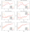Fig. D.1

Radial profiles of gaseous fractional abundances of CH₄ $n_{{CH}_{4}}$ $n_{\mathrm{CH}_{4}}$ /n_H (top panels),HCN n_HCN/n_H (middle panels), and C₂H $n_{C_{2} H}$ $n_{\mathrm{C}_{2}\mathrm{H}}$ /n_H (bottom panels) in NGC 1333-IRAS 2A (left) and NGC 1333-IRAS 4A (right) envelope models.

Appendix E NH₃ and N₂ fractional abundances

The top panels of Fig. E.1 show the radial profiles of NH₃ gas fractional abundances $n_{{NH}_{3}}$ $n_{\mathrm{NH}_{3}}$ /n_H in the IRAS 2A and IRAS 4A envelope models for the various X-ray luminosities. The binding energy of NH₃ is lower than that of H₂O and HCN, and higher than that of CO₂ (E_des(NH₃) = 2715 K, E_des(HCN) = 3610 K, E_des(CO₂) = 2267 K, and E_des(H₂O) = 4880 K, see Table 2), and the NH₃ snowline position exists outside the water snowline and the HCN snowline (> 2 × 10² au) and inside the CO₂ snowline (< 3 × 10² au). Zhang et al. (2018) discussed the possibility to observe the NH₃ line emission (the 23GHz 1,1 and 2,2 lines) with ngVLA as a proxy of the water snowline in disks.

According to Fig. E.1, for L_X ≳ 10³¹ erg s⁻¹, the NH₃ gas abundances increase (up to ~ 10⁻⁸–10⁻⁷) outside the NH₃ snowline, compared with the values (~ 10⁻⁹–10⁻⁸ in IRAS 2A and ~ 10⁻¹⁰–10⁻⁹ in IRAS 4A) for L_X ≲ 10³⁰ erg s⁻¹. The X-ray-induced photodesorption is considered important in this region. Inside the NH₃ snowline, for low X-ray luminosities, the NH₃ snowline gas abundances are around ~10⁻⁵. As the X-ray fluxes increase, the NH₃ snowline gas abundances in these radii decrease. For L_X ≳ 10³⁰ erg s⁻¹, the NH₃ gas abundances are ≲ 10⁻⁸–10⁻⁷ within the NH₃ snowline. The X-ray-induced photodissociation and ion-molecule reactions are considered the dominant destruction processes of NH₃ in the inner envelopes (e.g., Gredel et al. 1989; Walsh et al. 2015; Eistrup et al. 2016). Thus, with a strong X-ray field, the NH₃ abundance is no longer the dominant nitrogen carrier. In addition, it cannot be used as the tracer of the water snowline position since NH₃ gas abundances are similar within and outside the NH₃ snowline.

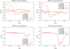Fig. E.1

Radial profiles of gaseous fractional abundances of NH₃ $n_{{NH}_{3}}$ $n_{\mathrm{NH}_{3}}$ /n_H (top panels) and N₂ $n_{N_{2}}$ $n_{\mathrm{N}_{2}}$ /n_H (bottom panels) in NGC 1333-IRAS 2A (left) and NGC 1333-IRAS 4A (right) envelope models.

The NH₃ line emission (e.g., the 23GHz (1,1), (2,2), and (3,3) lines) have been observed toward protostar disks and envelopes using VLA (e.g., Choi et al. 2007, 2010). However, the spatial resolutions of such VLA observations (~ 1.0′′) were not sufficient to resolve the inner structures around the protostars at a few hundred pc. Future ngVLA observations of these NH₃ lines with much higher resolutions (≲0.3′′ at around 23 GHz) will resolve the NH₃ gas emission within its snowline toward many protostars, and can also constrain the impact of X-rays on NH₃ gas abundances. In addition, such observations will be important to trace the chemical history of nitrogen-bearing molecules.

The bottom panels of Fig. E.1 show the radial profiles of N₂ gas fractional abundances $n_{N_{2}}$ $n_{\mathrm{N}_{2}}$ /n_H in the IRAS 2A and IRAS 4A envelope models for the various X-ray luminosities. As for CO, the N₂ gas abundances do not depend on X-ray fluxes.

Appendix F Fractional abundances and percentage contributions of major oxygen-bearing molecules

Table F.1 shows the fractional abundances of major oxygen-bearing molecules at r = 60 au (T_gas ~ 150 K, inside the water snowline) in the IRAS 2A and IRAS 4A envelope models for the various X-ray luminosities, and their percentage contributions (see also Figs. 8 and 9 in Sect. 4.1). The cutoff threshold is 0.01% for the contributions.

Table F.1

Fractional abundances of major oxygen-bearing molecules at r = 60 au (T_gas ~ 150 K, inside the water snowline) in the NGC 1333-IRAS 2A and NGC 1333-IRAS 4A envelope models for the various X-ray luminosities, and their percentage contributions relative to the total elemental oxygen abundance (3.2 × 10⁻⁴).

Appendix G Additional model calculations for X-ray-induced photodesorption rates

In Fig. G.1 and Fig. 11 in Sect. 4.3 we show the radial profiles of gaseous fractional abundances of H₂O, O₂, and OH, and icy fractional abundances of H₂O in the IRAS4A envelope models for our standard model calculations and additional model calculations. In Figs. G.2 and G.3 we show the radial profiles of gaseous fractional abundances of O, HCO⁺, and CH₃OH, and icy fractional abundances of CH₃OH in the IRAS4A envelope models for our standard model calculations and the additional model calculations. For the additional model calculations in Figs. G.1 and G.2, we include the photodesorption by UV photons generated internally via the interaction of secondary electrons produced by X-rays with H₂ molecules. For the additional model calculations in Fig. G.3 and Fig. 11 in Sect. 4.3, we switch off the direct X-ray-induced photodesorption and include the secondary (indirect) X-ray-induced photodesorption only.

According to Figs. G.1 and G.2, the effects of such additional secondary (indirect) X-ray-induced photodesorption is marginal (the abundances are changed by <1%, see also Sect. 4.3). For molecules shown in Fig. G.3, the differences in abundances between the standard model and the second additional model are much smaller than those in H₂O, OH, and O₂ (see Fig. 11 in Sect. 4.3).

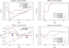Fig. G.1

Radial profiles of gaseous fractional abundances of H₂O, O₂, and OH, andicy fractional abundances of H₂O in the NGC 1333-IRAS 4A envelope models. The light green solid lines, the cyan double-dashed dotted lines, and the blue dotted lines show the radial profiles of our standard model calculations, for values of central star X-ray luminosities L_X =10²⁸, 10³⁰, and 10³² erg s⁻¹, respectively (see also Figs. 3, 4, 5, 6). The yellow dashed double-dotted lines, the scarlet dashed dotted lines, and the brown dashed lines show the radial profiles of our additional model calculations for L_X =10²⁸, 10³⁰, and 10³² erg s⁻¹, respectively. Included in the additional model calculations is the photodesorption by UV photons generated internally via the interaction of secondary electrons produced by X-rays with H₂ molecules (see also Fig. G.2). In the top left panel the observational best-fit H₂O gas abundance profile obtained in van Dishoeck et al. (2021) is overplotted with the black solid line (see also Fig. 10). In the bottom left panel the three model O₂ gas abundance profiles obtained in Yıldız et al. (2013) are overplotted (see also Fig. 10).

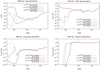Fig. G.2

Radial profiles of gaseous fractional abundances of O, HCO⁺, and CH₃OH, and icy fractional abundances of CH₃OH in the NGC1333-IRAS 4A envelope models. The line types and color patterns for the radial profiles of our standard model calculations (see also Figs. 5, 6, and 7) and additional model calculations are the same as in Fig. G.1. In the additional model calculations, we include the secondary (indirect) X-ray-induced photodesorption (see also Fig. G.1).

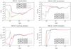Fig. G.3

Radial profiles of gaseous fractional abundances of O, HCO⁺, and CH₃OH, and icy fractional abundances of CH₃OH in the NGC 1333-IRAS 4A envelope models. The profiles are the same as in Fig. G.2, except in the additional model calculations the direct X-ray-induced photodesorption is switched off and only the secondary (indirect) X-ray-induced photodesorption is included (see also Fig. 11).

Appendix H Impacts of the different photodissociation branching ratio and binding energies on the molecular abundances

Figure H.1 shows the gas-phase abundance profiles of H₂O, O₂, O, and OH, which are calculated assuming the extreme case that the product of H₂O photodissociation is 100% atomic oxygen (Reaction (15) only both in the gas and ice). Figure H.2 shows the gas-phase abundance profiles of H₂O, O₂, O, and OH, which are obtained from our test calculations assuming the smaller E_des(O) (= 800 K) than that in our fiducial model (=1660 K).

We plotthese figures in order to investigate the impacts of the different photodissociation branching ratio of H₂O and different binding energies of O on the abundances of H₂O and related molecules. In Sect. 4.4, we discuss these impacts in detail (see also Fig. 12).

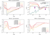Fig. H.1

Radial profiles of gaseous fractional abundances of H₂O, O₂, O, and OH in NGC 1333-IRAS 4A envelope models. These profiles are obtained from our test calculations assuming that the product of H₂O photodissociation is 100% atomic oxygen, unlike our fiducial model (100% OH). In the top left panel the observational best-fit H₂O gas abundance profile obtained in van Dishoeck et al. (2021) is overplotted with the black solid line (see also Fig. 10). In the top right panel the three model O₂ gas abundance profiles obtained in Yıldız et al. (2013) are overplotted (see also Fig. 10).

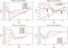Fig. H.2

Radial profiles of gaseous fractional abundances of H₂O, O₂, O, and OH in NGC 1333-IRAS 4A envelope models. These profiles are obtained from our test calculations assuming the smaller E_des(j) for atomic oxygen (=800 K) rather than that in our fiducial model (= 1660 K). In the top left panel the observational best-fit H₂O gas abundance profile obtained in van Dishoeck et al. (2021) is overplotted with the black solid line (see also Figs. 10 and H.1). In the top right panel the three model O₂ gas abundance profiles obtained in Yıldız et al. (2013) are overplotted (see also Figs. 10 and H.1).

References

Acharyya, K. 2014, MNRAS, 443, 1301 [Google Scholar]
Adams, N. G., Smith, D., & Grief, D. 1978, Int. J. Mass Spectr. Ion Process., 26, 405 [NASA ADS] [CrossRef] [Google Scholar]
Aikawa, Y., Miyama, S. M., Nakano, T., & Umebayashi, T. 1996, ApJ, 467, 684 [NASA ADS] [CrossRef] [Google Scholar]
Aikawa, Y., Umebayashi, T., Nakano, T., et al. 1999, ApJ, 519, 705 [NASA ADS] [CrossRef] [Google Scholar]
Aikawa, Y., Wakelam, V., Garrod, R. T., et al. 2008, ApJ, 674, 984 [NASA ADS] [CrossRef] [Google Scholar]
Aikawa, Y., Wakelam, V., Hersant, F., et al. 2012, ApJ, 760, 40 [NASA ADS] [CrossRef] [Google Scholar]
Aikawa, Y., Furuya, K., Yamamoto, S., et al. 2020, ApJ, 897, 110 [CrossRef] [Google Scholar]
Al-Halabi, A., & van Dishoeck, E. F. 2007, MNRAS, 382, 1648 [NASA ADS] [CrossRef] [Google Scholar]
Andrade, D. P. P., Rocco, M. L. M., & Boechat-Roberty, H. M. 2010, MNRAS, 409, 1289 [Google Scholar]
Ansdell, M., Williams, J. P., van der Marel, N., et al. 2016, ApJ, 828, 46 [Google Scholar]
Arakawa, S., & Krijt, S. 2021, ApJ, 910, 130 [CrossRef] [Google Scholar]
Arasa, C., Andersson, S., Cuppen, H. M., et al. 2010, J. Chem. Phys., 132, 184510 [NASA ADS] [CrossRef] [Google Scholar]
Arasa, C., Koning, J., Kroes, G.-J., et al. 2015, A&A, 575, A121 [NASA ADS] [CrossRef] [EDP Sciences] [Google Scholar]
Barzel, B., & Biham, O. 2007, ApJ, 658, L37 [NASA ADS] [CrossRef] [Google Scholar]
Basalgète, R., Dupuy, R., Féraud, G., et al. 2021a, A&A, 647, A35 [CrossRef] [EDP Sciences] [Google Scholar]
Basalgète, R., Dupuy, R., Féraud, G., et al. 2021b, A&A, 647, A36 [EDP Sciences] [Google Scholar]
Baulch, D. L., Cobos, C. J., Cox, R. A., et al. 1992, J. Phys. Chem. Ref. Data, 21, 411 [NASA ADS] [CrossRef] [Google Scholar]
Benz, A. O., Bruderer, S., van Dishoeck, E. F., et al. 2016, A&A, 590, A105 [NASA ADS] [CrossRef] [EDP Sciences] [Google Scholar]
Berger, M. J., Hubbell, J. H., Seltzer, S. M., Coursey, J. S., & Zucker, D. S. 1999, XCOM: Photon Cross Section Database (version 1.5). Online Available: https://www.nist.gov/pml/xcom-photon-cross-sections-database (National Institute of Standards and Technology, Gaithersburg, MD) [Google Scholar]
Bergner, J. B., Öberg, K. I., Bergin, E. A., et al. 2020, ApJ, 898, 97 [CrossRef] [Google Scholar]
Bertin, M., Romanzin, C., Doronin, M., et al. 2016, ApJ, 817, L12 [Google Scholar]
Bianchi, E., Chandler, C. J., Ceccarelli, C., et al. 2020, MNRAS, 498, L87 [CrossRef] [Google Scholar]
Bjerkeli, P., Jørgensen, J. K., Bergin, E. A., et al. 2016, A&A, 595, A39 [NASA ADS] [CrossRef] [EDP Sciences] [Google Scholar]
Boogert, A. C. A., Gerakines, P. A., & Whittet, D. C. B. 2015, ARA&A, 53, 541 [Google Scholar]
Boonman, A. M. S., van Dishoeck, E. F., Lahuis, F., et al. 2003, A&A, 399, 1063 [NASA ADS] [CrossRef] [EDP Sciences] [Google Scholar]
Bosman, A. D., Bruderer, S., & van Dishoeck, E. F. 2017, A&A, 601, A36 [NASA ADS] [CrossRef] [EDP Sciences] [Google Scholar]
Bosman, A. D., Tielens, A. G. G. M., & van Dishoeck, E. F. 2018a, A&A, 611, A80 [NASA ADS] [CrossRef] [EDP Sciences] [Google Scholar]
Bosman, A. D., Walsh, C., & van Dishoeck, E. F. 2018b, A&A, 618, A182 [NASA ADS] [CrossRef] [EDP Sciences] [Google Scholar]
Bruderer, S., Doty, S. D., & Benz, A. O. 2009, ApJS, 183, 179 [NASA ADS] [CrossRef] [Google Scholar]
Bruderer, S., Benz, A. O., Stäuber, P., et al. 2010, ApJ, 720, 1432 [NASA ADS] [CrossRef] [Google Scholar]
Cardelli, J. A., Savage, B. D., & Ebbets, D. C. 1991, ApJ, 383, L23 [Google Scholar]
Cardelli, J. A., Meyer, D. M., Jura, M., et al. 1996, ApJ, 467, 334 [NASA ADS] [CrossRef] [Google Scholar]
Carty, D., Goddard, A., Kahler, S. P. K., Sims, I. R., & Smith, I. W. M. 2006, J. Phys. Chem. A, 110, 3101 [Google Scholar]
Caselli, P., Hasegawa, T. I., & Herbst, E. 1998, ApJ, 495, 309 [Google Scholar]
Caselli, P., Keto, E., Bergin, E. A., et al. 2012, ApJ, 759, L37 [Google Scholar]
Ceccarelli, C., Dominik, C., López-Sepulcre, A., et al. 2014, ApJ, 790, L1 [NASA ADS] [CrossRef] [Google Scholar]
Charnley, S. B., Tielens, A. G. G. M., & Millar, T. J. 1992, ApJ, 399, L71 [Google Scholar]
Choi, M., Tatematsu, K., Park, G., et al. 2007, ApJ, 667, L183 [Google Scholar]
Choi, M., Tatematsu, K., & Kang, M. 2010, ApJ, 723, L34 [Google Scholar]
Chuang, K.-J., Fedoseev, G., Ioppolo, S., et al. 2016, MNRAS, 455, 1702 [Google Scholar]
Cieza, L. A., Casassus, S., Tobin, J., et al. 2016, Nature, 535, 258 [Google Scholar]
Cleeves, L. I., Bergin, E. A., & Adams, F. C. 2014, ApJ, 794, 123 [NASA ADS] [CrossRef] [Google Scholar]
Cleeves, L. I., Bergin, E. A., Öberg, K. I., et al. 2017, ApJ, 843, L3 [NASA ADS] [CrossRef] [Google Scholar]
Collings, M. P., Anderson, M. A., Chen, R., et al. 2004, MNRAS, 354, 1133 [NASA ADS] [CrossRef] [Google Scholar]
Coutens, A., Vastel, C., Caux, E., et al. 2012, A&A, 539, A132 [NASA ADS] [CrossRef] [EDP Sciences] [Google Scholar]
Coutens, A., Vastel, C., Cabrit, S., et al. 2013, A&A, 560, A39 [NASA ADS] [CrossRef] [EDP Sciences] [Google Scholar]
Coutens, A., Commerçon, B., & Wakelam, V. 2020, A&A, 643, A108 [EDP Sciences] [Google Scholar]
Crownover, R. L., De Lucia, F. C., & Herbst, E. 1990, ApJ, 349, L29 [Google Scholar]
Cruz-Diaz, G. A., Martín-Doménech, R., Muñoz Caro, G. M., et al. 2016, A&A, 592, A68 [NASA ADS] [CrossRef] [EDP Sciences] [Google Scholar]
Cuppen, H. M., van Dishoeck, E. F., Herbst, E., et al. 2009, A&A, 508, 275 [NASA ADS] [CrossRef] [EDP Sciences] [Google Scholar]
Cuppen, H. M., Ioppolo, S., Romanzin, C., et al. 2010, Physical Chemistry Chemical Physics (Incorporating Faraday Transactions), 1212077 [Google Scholar]
Cuppen, H. M., Walsh, C., Lamberts, T., et al. 2017, Space Sci. Rev., 212, 1 [Google Scholar]
De Simone, M., Ceccarelli, C., Codella, C., et al. 2020, ApJ, 896, L3 [CrossRef] [Google Scholar]
Drozdovskaya, M. N., Walsh, C., Visser, R., et al. 2014, MNRAS, 445, 913 [Google Scholar]
Drozdovskaya, M. N., Walsh, C., van Dishoeck, E. F., et al. 2016, MNRAS, 462, 977 [Google Scholar]
Dulieu, F., Congiu, E., Noble, J., et al. 2013, Scientific Rep., 3, 1338 [Google Scholar]
Dunham, M. M., Stutz, A. M., Allen, L. E., et al. 2014, in Protostars and Planets VI, ed. H. Beuther et al. (Tucson, AZ: Univ. Arizona Press), 195 [Google Scholar]
Dupuy, R., Bertin, M., Féraud, G., et al. 2018, Nat. Astron., 2, 796 [Google Scholar]
Eistrup, C., & Walsh, C. 2019, A&A, 621, A75 [CrossRef] [EDP Sciences] [Google Scholar]
Eistrup, C., Walsh, C., & van Dishoeck, E. F. 2016, A&A, 595, A83 [NASA ADS] [CrossRef] [EDP Sciences] [Google Scholar]
Eistrup, C., Walsh, C., & van Dishoeck, E. F. 2018, A&A, 613, A14 [NASA ADS] [CrossRef] [EDP Sciences] [Google Scholar]
Enoch, M. L., Evans, N. J., Sargent, A. I., et al. 2008, ApJ, 684, 1240 [Google Scholar]
Evans, N. J., Dunham, M. M., Jørgensen, J. K., et al. 2009, ApJS, 181, 321 [Google Scholar]
Favre, C., López-Sepulcre, A., Ceccarelli, C., et al. 2017, A&A, 608, A82 [NASA ADS] [CrossRef] [EDP Sciences] [Google Scholar]
Fillion, J.-H., Fayolle, E. C., Michaut, X., et al. 2014, Faraday Discuss., 168, 533 [Google Scholar]
Forbrich, J., Preibisch, T., & Menten, K. M. 2006, A&A, 446, 155 [NASA ADS] [CrossRef] [EDP Sciences] [Google Scholar]
Fuchs, G. W., Cuppen, H. M., Ioppolo, S., et al. 2009, A&A, 505, 629 [NASA ADS] [CrossRef] [EDP Sciences] [Google Scholar]
Furuya, K., & Aikawa, Y. 2014, ApJ, 790, 97 [NASA ADS] [CrossRef] [Google Scholar]
Furuya, K., van Dishoeck, E. F., & Aikawa, Y. 2016, A&A, 586, A127 [NASA ADS] [CrossRef] [EDP Sciences] [Google Scholar]
Furuya, K., Drozdovskaya, M. N., Visser, R., et al. 2017, A&A, 599, A40 [NASA ADS] [CrossRef] [EDP Sciences] [Google Scholar]
Garrod, R. T. 2008, A&A, 491, 239 [NASA ADS] [CrossRef] [EDP Sciences] [Google Scholar]
Garrod, R. T., & Herbst, E. 2006, A&A, 457, 927 [NASA ADS] [CrossRef] [EDP Sciences] [Google Scholar]
Garrod, R. T., & Pauly, T. 2011, ApJ, 735, 15 [NASA ADS] [CrossRef] [Google Scholar]
Garrod, R. T., Widicus Weaver, S. L., & Herbst, E. 2008, ApJ, 682, 283 [NASA ADS] [CrossRef] [Google Scholar]
Garrod, R. T., Vasyunin, A. I., Semenov, D. A., et al. 2009, ApJ, 700, L43 [Google Scholar]
Geppert, W. D., Hamberg, M., Thomas, R. D., et al. 2006, Faraday Discuss., 133, 177 [Google Scholar]
Giardino, G., Favata, F., Micela, G., et al. 2007, A&A, 463, 275 [NASA ADS] [CrossRef] [EDP Sciences] [Google Scholar]
Graedel, T. E., Langer, W. D., & Frerking, M. A. 1982, ApJS, 48, 321 [NASA ADS] [CrossRef] [Google Scholar]
Gredel, R., Lepp, S., & Dalgarno, A. 1987, ApJ, 323, L137 [Google Scholar]
Gredel, R., Lepp, S., Dalgarno, A., et al. 1989, ApJ, 347, 289 [Google Scholar]
Grosso, N., Hamaguchi, K., Principe, D. A., et al. 2020, A&A, 638, L4 [EDP Sciences] [Google Scholar]
Glassgold, A. E., Najita, J., & Igea, J. 1997, ApJ, 480, 344 [Google Scholar]
Güdel, M., & Nazé, Y. 2009, A&ARv, 17, 309 [NASA ADS] [CrossRef] [Google Scholar]
Hamaguchi, K., Corcoran, M. F., Petre, R., et al. 2005, ApJ, 623, 291 [Google Scholar]
Harsono, D., Jørgensen, J. K., van Dishoeck, E. F., et al. 2014, A&A, 562, A77 [NASA ADS] [CrossRef] [EDP Sciences] [Google Scholar]
Harsono, D., Bruderer, S., & van Dishoeck, E. F. 2015, A&A, 582, A41 [NASA ADS] [CrossRef] [EDP Sciences] [Google Scholar]
Harsono, D., Persson, M. V., Ramos, A., et al. 2020, A&A, 636, A26 [CrossRef] [EDP Sciences] [Google Scholar]
Hasegawa, T. I., & Herbst, E. 1993, MNRAS, 261, 83 [NASA ADS] [CrossRef] [Google Scholar]
Hasegawa, T. I., Herbst, E., & Leung, C. M. 1992, ApJS, 82, 167 [NASA ADS] [CrossRef] [Google Scholar]
Hassel, G. E., Herbst, E., & Garrod, R. T. 2008, ApJ, 681, 1385 [Google Scholar]
He, J., & Vidali, G. 2014, ApJ, 788, 50 [Google Scholar]
He, J., Jing, D., & Vidali, G. 2014, Phys. Chem. Chem. Phys., 16, 3493 [Google Scholar]
Heays, A. N., Bosman, A. D., & van Dishoeck, E. F. 2017, A&A, 602, A105 [NASA ADS] [CrossRef] [EDP Sciences] [Google Scholar]
Heinzeller, D., Nomura, H., Walsh, C., & Millar, T. J. 2011, ApJ, 731, 115 [NASA ADS] [CrossRef] [Google Scholar]
Henning, T., Semenov, D., Guilloteau, S., et al. 2010, ApJ, 714, 1511 [Google Scholar]
Herbst, E., & van Dishoeck, E. F. 2009, ARA&A, 47, 427 [NASA ADS] [CrossRef] [Google Scholar]
Herczeg, G. J., Johnstone, D., Mairs, S., et al. 2017, ApJ, 849, 43 [Google Scholar]
Higuchi, A. E., Sakai, N., Watanabe, Y., et al. 2018, ApJS, 236, 52 [Google Scholar]
Hofner, P., & Churchwell, E. 1997, ApJ, 486, L39 [Google Scholar]
Hogerheijde, M. R., & van der Tak, F. F. S. 2000, A&A, 362, 697 [NASA ADS] [Google Scholar]
Hollenbach, D., Kaufman, M. J., Bergin, E. A., et al. 2009, ApJ, 690, 1497 [Google Scholar]
Hodapp, K. W., Chini, R., Watermann, R., et al. 2012, ApJ, 744, 56 [Google Scholar]
Hsieh, T.-H., Murillo, N. M., Belloche, A., et al. 2019, ApJ, 884, 149 [NASA ADS] [CrossRef] [Google Scholar]
Huntress, W. T. 1977, ApJS, 33, 495 [Google Scholar]
Igea, J., & Glassgold, A. E. 1999, ApJ, 518, 848 [Google Scholar]
Imai, M., Sakai, N., Oya, Y., et al. 2016, ApJ, 830, L37 [NASA ADS] [CrossRef] [Google Scholar]
Imanishi, K., Koyama, K., & Tsuboi, Y. 2001, ApJ, 557, 747 [Google Scholar]
Ivezic, Z., & Elitzur, M. 1997, MNRAS, 287, 799 [Google Scholar]
Jensen, S. S., Jørgensen, J. K., Kristensen, L. E., et al. 2019, A&A, 631, A25 [Google Scholar]
Jørgensen, J. K., & van Dishoeck, E. F. 2010, ApJ, 710, L72 [NASA ADS] [CrossRef] [Google Scholar]
Jørgensen, J. K., Bourke, T. L., Myers, P. C., et al. 2007, ApJ, 659, 479 [NASA ADS] [CrossRef] [Google Scholar]
Jørgensen, J. K., van Dishoeck, E. F., Visser, R., et al. 2009, A&A, 507, 861 [NASA ADS] [CrossRef] [EDP Sciences] [Google Scholar]
Jørgensen, J. K., Visser, R., Sakai, N., et al. 2013, ApJ, 779, L22 [NASA ADS] [CrossRef] [Google Scholar]
Jørgensen, J. K., Belloche, A., & Garrod, R. T. 2020, ARA&A, 58, 727 [Google Scholar]
Kamezaki, T., Imura, K., Omodaka, T., et al. 2014, ApJS, 211, 18 [Google Scholar]
Karska, A., Herczeg, G. J., van Dishoeck, E. F., et al. 2013, A&A, 552, A141 [NASA ADS] [CrossRef] [EDP Sciences] [Google Scholar]
Koumpia, E., Semenov, D. A., van der Tak, F. F. S., et al. 2017, A&A, 603, A88 [NASA ADS] [CrossRef] [EDP Sciences] [Google Scholar]
Krijt, S., Bosman, A. D., Zhang, K., et al. 2020, ApJ, 899, 134 [Google Scholar]
Kristensen, L. E., & Dunham, M. M. 2018, A&A, 618, A158 [NASA ADS] [CrossRef] [EDP Sciences] [Google Scholar]
Kristensen, L. E., Visser, R., van Dishoeck, E. F., et al. 2010, A&A, 521, L30 [NASA ADS] [CrossRef] [EDP Sciences] [Google Scholar]
Kristensen, L. E., van Dishoeck, E. F., Bergin, E. A., et al. 2012, A&A, 542, A8 [NASA ADS] [CrossRef] [EDP Sciences] [Google Scholar]
Kristensen, L. E., Gusdorf, A., Mottram, J. C., et al. 2017, A&A, 601, L4 [CrossRef] [EDP Sciences] [Google Scholar]
Lamberts, T., Cuppen, H. M., Ioppolo, S., et al. 2013, Phys. Chem. Chem. Phys., 15, 8287 [Google Scholar]
Lee, J.-E., Lee, S., Baek, G., et al. 2019, Nat. Astron., 3, 314 [NASA ADS] [CrossRef] [Google Scholar]
Lee, S., Lee, J.-E., Aikawa, Y., et al. 2020, ApJ, 889, 20 [Google Scholar]
Leemker, M., van’t Hoff, M. L. R., Trapman, L., et al. 2021, A&A, 646, A3 [EDP Sciences] [Google Scholar]
Leger, A., Jura, M., & Omont, A. 1985, A&A, 144, 147 [Google Scholar]
Li, J. I.-H., Liu, H. B., Hasegawa, Y., et al. 2017, ApJ, 840, 72 [Google Scholar]
Long, F., Herczeg, G. J., Pascucci, I., et al. 2017, ApJ, 844, 99 [NASA ADS] [CrossRef] [Google Scholar]
Maloney, P. R., Hollenbach, D. J., & Tielens, A. G. G. M. 1996, ApJ, 466, 561 [Google Scholar]
Marboeuf, U., Thiabaud, A., Alibert, Y., et al. 2014, A&A, 570, A35 [NASA ADS] [CrossRef] [EDP Sciences] [Google Scholar]
McElroy, D., Walsh, C., Markwick, A. J., et al. 2013, A&A, 550, A36 [NASA ADS] [CrossRef] [EDP Sciences] [Google Scholar]
Melnick, G. J., Tolls, V., Snell, R. L., et al. 2020, ApJ, 892, 22 [CrossRef] [Google Scholar]
Meyer, D. M., Jura, M., & Cardelli, J. A. 1998, ApJ, 493, 222 [Google Scholar]
Miotello, A., Testi, L., Lodato, G., et al. 2014, A&A, 567, A32 [NASA ADS] [CrossRef] [EDP Sciences] [Google Scholar]
Mottram, J. C., van Dishoeck, E. F., Schmalzl, M., et al. 2013, A&A, 558, A126 [NASA ADS] [CrossRef] [EDP Sciences] [Google Scholar]
Neufeld, D. A., Lepp, S., & Melnick, G. J. 1995, ApJS, 100, 132 [NASA ADS] [CrossRef] [Google Scholar]
Nisini, B., Santangelo, G., Giannini, T., et al. 2015, ApJ, 801, 121 [Google Scholar]
Noble, J. A., Congiu, E., Dulieu, F., et al. 2012, MNRAS, 421, 768 [Google Scholar]
Noble, J. A., Theule, P., Congiu, E., et al. 2015, A&A, 576, A91 [NASA ADS] [CrossRef] [EDP Sciences] [Google Scholar]
Nomura, H., & Millar, T. J. 2004, A&A, 414, 409 [NASA ADS] [CrossRef] [EDP Sciences] [MathSciNet] [Google Scholar]
Nomura, H., Aikawa, Y., Tsujimoto, M., Nakagawa, Y., & Millar, T. J. 2007, ApJ, 661, 334 [Google Scholar]
Nomura, H., Aikawa, Y., Nakagawa, Y., et al. 2009, A&A, 495, 183 [NASA ADS] [CrossRef] [EDP Sciences] [Google Scholar]
Notsu, S., Nomura, H., Ishimoto, D., et al. 2016, ApJ, 827, 113 [Google Scholar]
Notsu, S., Nomura, H., Ishimoto, D., et al. 2017, ApJ, 836, 118 [Google Scholar]
Notsu, S., Nomura, H., Walsh, C., et al. 2018, ApJ, 855, 62 [Google Scholar]
Notsu, S., Akiyama, E., Booth, A., et al. 2019, ApJ, 875, 96 [Google Scholar]
Notsu, S., Eistrup, C., Walsh, C., & Nomura, H. 2020, MNRAS, 499, 2229 [Google Scholar]
Öberg, K. I., & Bergin, E. A. 2021, Phys. Rep., 893, 1 [Google Scholar]
Öberg, K. I., van Broekhuizen, F., Fraser, H. J., et al. 2005, ApJ, 621, L33 [NASA ADS] [CrossRef] [Google Scholar]
Öberg, K. I., Fuchs, G. W., Awad, Z., et al. 2007, ApJ, 662, L23 [Google Scholar]
Öberg, K. I., van Dishoeck, E. F., & Linnartz, H. 2009a, A&A, 496, 281 [NASA ADS] [CrossRef] [EDP Sciences] [Google Scholar]
Öberg, K. I., Linnartz, H., Visser, R., & van Dishoeck, E. F. 2009b, ApJ, 693, 1209 [NASA ADS] [CrossRef] [Google Scholar]
Öberg, K. I., Garrod, R. T., van Dishoeck, E. F., & Linnartz, H. 2009c, A&A, 504, 891 [NASA ADS] [CrossRef] [EDP Sciences] [Google Scholar]
Öberg, K. I., Boogert, A. C. A., Pontoppidan, K. M., et al. 2011, ApJ, 740, 109 [NASA ADS] [CrossRef] [Google Scholar]
Öberg, K. I., Cleeves, L. I., & Loomis, R. 2018, in Monograph 7, Science with a Next Generation Very Large Array, Eric ed. J. Murphy, (San Francisco, CA: ASP), Astronomical Society of the Pacific Conference Series, 223 [Google Scholar]
Okuzumi, S., & Tazaki, R. 2019, ApJ, 878, 132 [Google Scholar]
Okuzumi, S., Tanaka, H., Kobayashi, H., et al. 2012, ApJ, 752, 106 [Google Scholar]
Oldenborg, R. C., Loge, G. W., Harradine, D. M., & Winn, K. R. 1992, J. Phys. Chem., 96, 8426 [Google Scholar]
Ormel, C. W., Paszun, D., Dominik, C., et al. 2009, A&A, 502, 845 [NASA ADS] [CrossRef] [EDP Sciences] [Google Scholar]
Oya, Y., Sakai, N., López-Sepulcre, A., et al. 2016, ApJ, 824, 88 [Google Scholar]
Padovani, M., Marcowith, A., Hennebelle, P., et al. 2016, A&A, 590, A8 [NASA ADS] [CrossRef] [EDP Sciences] [Google Scholar]
Prasad, S. S., & Tarafdar, S. P. 1983, ApJ, 267, 603 [Google Scholar]
Penteado, E. M., Walsh, C., & Cuppen, H. M. 2017, ApJ, 844, 71 [NASA ADS] [CrossRef] [Google Scholar]
Persson, M. V., Jørgensen, J. K., & van Dishoeck, E. F. 2012, A&A, 541, A39 [NASA ADS] [CrossRef] [EDP Sciences] [Google Scholar]
Persson, M. V., Jørgensen, J. K., & van Dishoeck, E. F. 2013, A&A, 549, L3 [NASA ADS] [CrossRef] [EDP Sciences] [Google Scholar]
Persson, M. V., Jørgensen, J. K., van Dishoeck, E. F., et al. 2014, A&A, 563, A74 [NASA ADS] [CrossRef] [EDP Sciences] [Google Scholar]
Persson, M. V., Harsono, D., Tobin, J. J., et al. 2016, A&A, 590, A33 [NASA ADS] [CrossRef] [EDP Sciences] [Google Scholar]
Poteet, C. A., Pontoppidan, K. M., Megeath, S. T., et al. 2013, ApJ, 766, 117 [Google Scholar]
Preibisch, T. 2003, A&A, 410, 951 [NASA ADS] [CrossRef] [EDP Sciences] [Google Scholar]
Preibisch, T., Kim, Y.-C., Favata, F., et al. 2005, ApJS, 160, 401 [Google Scholar]
Sahu, D., Liu, S.-Y., Su, Y.-N., et al. 2019, ApJ, 872, 196 [Google Scholar]
Sakai, N., & Yamamoto, S. 2013, Chem. Rev., 113, 8981 [Google Scholar]
Sakai, N., Sakai, T., Hirota, T., et al. 2008, ApJ, 672, 371 [Google Scholar]
Schöier, F. L., Jørgensen, J. K., van Dishoeck, E. F., et al. 2002, A&A, 390, 1001 [NASA ADS] [CrossRef] [EDP Sciences] [Google Scholar]
Schoonenberg, D., & Ormel, C. W. 2017, A&A, 602, A21 [NASA ADS] [CrossRef] [EDP Sciences] [Google Scholar]
Schmalzl, M., Visser, R., Walsh, C., et al. 2014, A&A, 572, A81 [NASA ADS] [CrossRef] [EDP Sciences] [Google Scholar]
Schwarz, K. R., Bergin, E. A., Cleeves, L. I., et al. 2018, ApJ, 856, 85 [NASA ADS] [CrossRef] [Google Scholar]
Schwarz, K. R., Bergin, E. A., Cleeves, L. I., et al. 2019, ApJ, 877, 131 [NASA ADS] [CrossRef] [Google Scholar]
Smith, R. S., May, R. A., & Kay, B. D. 2016, J. Phys. Chem. B, 120, 1979 [Google Scholar]
Stäuber, P., Doty, S. D., van Dishoeck, E. F., et al. 2005, A&A, 440, 949 [NASA ADS] [CrossRef] [EDP Sciences] [Google Scholar]
Stäuber, P., Jørgensen, J. K., van Dishoeck, E. F., et al. 2006, A&A, 453, 555 [NASA ADS] [CrossRef] [EDP Sciences] [Google Scholar]
Stantcheva, T., & Herbst, E. 2004, A&A, 423, 241 [NASA ADS] [CrossRef] [EDP Sciences] [Google Scholar]
Stäuber, P., Benz, A. O., Jørgensen, J. K., et al. 2007, A&A, 466, 977 [NASA ADS] [CrossRef] [EDP Sciences] [Google Scholar]
Taquet, V., Charnley, S. B., & Sipilä, O. 2014, ApJ, 791, 1 [Google Scholar]
Taquet, V., Wirström, E. S., & Charnley, S. B. 2016a, ApJ, 821, 46 [NASA ADS] [CrossRef] [Google Scholar]
Taquet, V., Furuya, K., Walsh, C., et al. 2016b, MNRAS, 462, S99 [Google Scholar]
Taquet, V., van Dishoeck, E. F., Swayne, M., et al. 2018, A&A, 618, A11 [NASA ADS] [CrossRef] [EDP Sciences] [Google Scholar]
Takasao, S., Tomida, K., Iwasaki, K., et al. 2019, ApJ, 878, L10 [Google Scholar]
Tielens, A. G. G. M., & Hagen, W. 1982, A&A, 114, 245 [Google Scholar]
Turrini, D., Schisano, E., Fonte, S., et al. 2021, ApJ, 909, 40 [Google Scholar]
Umebayashi, T., & Nakano, T. 2009, ApJ, 690, 69 [Google Scholar]
van Dishoeck, E. F., Helmich, F. P., de Graauw, T., et al. 1996, A&A, 315, L349 [NASA ADS] [Google Scholar]
van Dishoeck, E. F., Jonkheid, B., & van Hemert, M. C. 2006, Faraday Discuss., 133, 231 [Google Scholar]
van Dishoeck, E. F., Kristensen, L. E., Benz, A. O., et al. 2011, PASP, 123, 138 [Google Scholar]
van Dishoeck, E. F., Herbst, E., & Neufeld, D. A. 2013, Chem. Rev., 113, 9043 [NASA ADS] [CrossRef] [PubMed] [Google Scholar]
van Dishoeck, E. F., Bergin, E. A., Lis, D. C., & Lunine, J. I. 2014, in Protostars and Planets VI, ed. H. Beuther et al. (Tucson, AZ: Univ. Arizona Press), 835 [Google Scholar]
van Dishoeck, E. F., Kristensen, L. E., Mottram, J. C., et al. 2021, A&A, 648, A24 [CrossRef] [EDP Sciences] [Google Scholar]
van Harrevelt, R., & van Hemert, M. C. 2008, J. Phys. Chem. A, 112, 3002 [CrossRef] [Google Scholar]
van ’t Hoff, M. L. R., Persson, M. V., Harsono, D., et al. 2018a, A&A, 613, A29 [NASA ADS] [CrossRef] [EDP Sciences] [Google Scholar]
van ’t Hoff, M. L. R., Tobin, J. J., Trapman, L., et al. 2018b, ApJ, 864, L23 [Google Scholar]
van’t Hoff, M. L. R., Harsono, D., Tobin, J. J., et al. 2020, ApJ, 901, 166 [CrossRef] [Google Scholar]
Vasyunin, A. I., & Herbst, E. 2013, ApJ, 762, 86 [Google Scholar]
Vasyunin, A. I., Semenov, D. A., Wiebe, D. S., et al. 2009, ApJ, 691, 1459 [Google Scholar]
Verner, D. A., Yakovlev, D. G., Band, I. M., et al. 1993, Atomic Data Nuclear Data Tables, 55, 233 [Google Scholar]
Visser, R., van Dishoeck, E. F., Doty, S. D., et al. 2009, A&A, 495, 881 [NASA ADS] [CrossRef] [EDP Sciences] [Google Scholar]
Visser, R., Doty, S. D., & van Dishoeck, E. F. 2011, A&A, 534, A132 [NASA ADS] [CrossRef] [EDP Sciences] [Google Scholar]
Visser, R., Kristensen, L. E., Bruderer, S., et al. 2012, A&A, 537, A55 [NASA ADS] [CrossRef] [EDP Sciences] [Google Scholar]
Visser, R., Jørgensen, J. K., Kristensen, L. E., et al. 2013, ApJ, 769, 19 [Google Scholar]
Visser, R., Bergin, E. A., & Jørgensen, J. K. 2015, A&A, 577, A102 [NASA ADS] [CrossRef] [EDP Sciences] [Google Scholar]
Wada, K., Tanaka, H., Okuzumi, S., et al. 2013, A&A, 559, A62 [NASA ADS] [CrossRef] [EDP Sciences] [Google Scholar]
Waggoner, A. R., & Cleeves, L. I. 2019, ApJ, 883, 197 [Google Scholar]
Walsh, C., Millar, T. J., & Nomura, H. 2010, ApJ, 722, 1607 [Google Scholar]
Walsh, C., Nomura, H., Millar, T. J., et al. 2012, ApJ, 747, 114 [Google Scholar]
Walsh, C., Millar, T. J., Nomura, H., et al. 2014a, A&A, 563, A33 [NASA ADS] [CrossRef] [EDP Sciences] [Google Scholar]
Walsh, C., Herbst, E., Nomura, H., et al. 2014b, Faraday Discuss., 168, 389 [Google Scholar]
Walsh, C., Nomura, H., & van Dishoeck, E. 2015, A&A, 582, A88 [NASA ADS] [CrossRef] [EDP Sciences] [Google Scholar]
Walsh, C., Loomis, R. A., Öberg, K. I., et al. 2016, ApJ, 823, L10 [Google Scholar]
Walsh, C., Vissapragada, S., & McGee, H. 2018, Proceedings of the International Astronomical Union, IAU Symp., 332, 395 [Google Scholar]
Watanabe, N., & Kouchi, A. 2002, ApJ, 571, L173 [Google Scholar]
Whittet, D. C. B. 2010, ApJ, 710, 1009 [NASA ADS] [CrossRef] [Google Scholar]
Woitke, P., Thi, W.-F., Kamp, I., et al. 2009, A&A, 501, L5 [NASA ADS] [CrossRef] [EDP Sciences] [Google Scholar]
Woods, P. M., Slater, B., Raza, Z., et al. 2013, ApJ, 777, 90 [Google Scholar]
Yang, Y.-L., Sakai, N., Zhang, Y., et al. 2021, ApJ, 910, 20 [Google Scholar]
Yıldız, U. A., Kristensen, L. E., van Dishoeck, E. F., et al. 2012, A&A, 542, A86 [NASA ADS] [CrossRef] [EDP Sciences] [Google Scholar]
Yıldız, U. A., Acharyya, K., Goldsmith, P. F., et al. 2013, A&A, 558, A58 [NASA ADS] [CrossRef] [EDP Sciences] [Google Scholar]
Yoneda, H., Tsukamoto, Y., Furuya, K., et al. 2016, ApJ, 833, 105 [Google Scholar]
Yoo, H., Lee, J.-E., Mairs, S., et al. 2017, ApJ, 849, 69 [Google Scholar]
Yu, M., Willacy, K., Dodson-Robinson, S. E., et al. 2016, ApJ, 822, 53 [Google Scholar]
Zhang, K., Bergin, E. A., Williams, J. P., et al. 2018, in Monograph 7, Science with a Next Generation Very Large Array, Eric J. Murphy, ed. (San Francisco, CA: ASP), Astronomical Society of the Pacific Conference Series, 209 [Google Scholar]
Zhang, K., Bergin, E. A., Schwarz, K., et al. 2019, ApJ, 883, 98 [Google Scholar]
Zhang, K., Schwarz, K. R., & Bergin, E. A. 2020, ApJ, 891, L17 [CrossRef] [Google Scholar]

¹

IRAM Plateau de Bure Interferometer, now NOEMA (NOrthern Extended Millimeter Array).

²

Atacama Large Millimeter/submillimeter Array.

³

Herschel Space Observatory.

⁴

In the remainder of this paper, we refer to NGC 1333-IRAS 2A and NGC 1333-IRAS 4A as “IRAS 2A” and “IRAS 4A”, respectively.

⁵

http://udfa.ajmarkwick.net

⁶

$n_{{HCO}^{+}}$ $n_{\mathrm{HCO}^{+}}$ is the number density of HCO⁺, and we obtain the value in Sect. 3.3 and Fig. 6.

⁷

http://faust-alma.riken.jp

⁸

The next generation Very Large Array.

⁹

For the definition of the values of low, moderate, and high X-ray luminosities, see Sect. 3.2.

All Tables

Table 1

UV photodesorption yields.

In the text

Table 2

Initial abundances for dominant molecules in our protostellar envelope models and their binding energies.

In the text

Table F.1

Fractional abundances of major oxygen-bearing molecules at r = 60 au (T_gas ~ 150 K, inside the water snowline) in the NGC 1333-IRAS 2A and NGC 1333-IRAS 4A envelope models for the various X-ray luminosities, and their percentage contributions relative to the total elemental oxygen abundance (3.2 × 10⁻⁴).

In the text

All Figures

Fig. 1

Radial profiles of molecular hydrogen number densities $n_{H_{2}}$ $n_{\mathrm{H}_{2}}$ (cm⁻³) and gas temperature T_gas (K) in NGC 1333-IRAS 2A and NGC 1333-IRAS 4A envelope models. The blue solid line and red dashed line show radial $n_{H_{2}}$ $n_{\mathrm{H}_{2}}$ profiles in IRAS 2A and IRAS 4A envelope models, respectively. The blue dotted line and red dash-dotted line show radial T_gas profiles in IRAS 2A and IRAS 4A envelope models, respectively.

In the text

Fig. 2

Radial profiles of the X-ray flux F_X(r) (erg s⁻¹ cm⁻²) (top panels) and the secondary X-ray ionization rate ξ_X(r) (s⁻¹) (bottom panels) in NGC 1333-IRAS 2A (left) and NGC 1333-IRAS 4A (right) envelope models. In the bottom panels, the horizontal gray solid lines show the assumed constant cosmic-ray ionization rate ξ_CR (r) = 1.0 × 10⁻¹⁷ s⁻¹. In all panels the different line styles and colors in the radial F_X(r) and ξ_X (r) profiles denote models with different central star X-ray luminosities L_X.

In the text

Fig. 3

Radial profiles of water gas fractional abundances with respect to total hydrogen nuclei densities $n_{H_{2} O}$ $n_{\mathrm{H}_{2}\mathrm{O}}$ /n_H for the whole envelopes on a log scale (top panels) and the inner regions only (r < 200 au) on a linear scale (bottom panels) in NGC 1333-IRAS 2A (left) and NGC 1333-IRAS 4A (right) envelope models. The double-dashed double-dotted lines, the dashed double-dotted lines, the double-dashed dotted lines, the dash-dotted lines, the dotted lines, the dashed lines, and the solid lines show the radial $n_{H_{2} O}$ $n_{\mathrm{H}_{2}\mathrm{O}}$ /n_H profiles for values of central star X-ray luminosities L_X = 0, 10²⁷, 10²⁸, 10²⁹, 10³⁰, 10³¹, and 10³² erg s⁻¹, respectively. The line color gradually changes from green to yellow, orange, red, and brown as the value of L_X increases. In Figs. 5–7, C.1, C.2, D.1, E.1, H.1, and H.2, we adopt the same line types and color patterns of the calculated radial fractional abundance profiles of gas-phase molecules for different values of L_X.

In the text

Fig. 4

Radial profiles of water ice fractional abundances $n_{H_{2} O, ice}$ $n_{\mathrm{H}_{2}\mathrm{O}, \mathrm{ice}}$ /n_H in NGC1333-IRAS 2A (left panel) and NGC 1333-IRAS 4A (right panel) envelope models. The line color gradually changes from green to cyan, blue, and indigo as the value of L_X increases. The profiles for L_X = 0−10²⁹ erg s⁻¹ almost overlap. In Figs. 7, C.1, and C.2, we adopt the same line types and color patterns of the radial fractional abundance profiles of icy-phase molecules for different values of L_X.

In the text

	Fig. 5 Radial profiles of the gaseous fractional abundances of molecular oxygen $n_{O_{2}}$ $n_{\mathrm{O}_{2}}$ /n_H (top panels) and atomic oxygen n_O/n_H (bottom panels) in NGC 1333-IRAS 2A (left) and NGC 1333-IRAS 4A (right) envelope models.
In the text

	Fig. 6 Radial profiles of the gaseous fractional abundances of HCO⁺ $n_{{HCO}^{+}}$ $n_{\mathrm{HCO}^{+}}$ /n_H (top panels) and OH n_OH/n_H (bottom panels) in NGC 1333- IRAS 2A (left) and NGC 1333-IRAS 4A (right) envelope models.
In the text

	Fig. 7 Radial profiles of methanol gas and ice fractional abundances $n_{{CH}_{3} OH}$ $n_{\mathrm{CH}_{3}\mathrm{OH}}$ /n_H (top panels) and $n_{{CH}_{3} OH, ice}$ $n_{\mathrm{CH}_{3}\mathrm{OH},\mathrm{ice}}$ /n_H (bottom panels) in NGC 1333-IRAS 2A (left) and NGC 1333-IRAS 4A (right) envelope models.
In the text

Fig. 8

Radial profiles of percentage contributions of the dominant oxygen-bearing molecules to the total elemental oxygen abundance (=3.2 × 10⁻⁴) in the NGC 1333-IRAS 2A envelope model (left panels) and the NGC 1333-IRAS 4A envelope model (right panels). The top, middle, and bottom panels show the radial profiles with L_X = 10²⁸, 10³⁰, and 10³² erg s⁻¹, respectively. The red, blue, purple, black, and green line profiles respectively show the contribution of CO, H₂O, O, O₂, and CO₂ molecules. The solid and dashed line profiles show the contribution of gaseous and icy molecules. Since O₂ and CO₂ include two oxygen atoms per molecule, the percentage contributions are twice as high as those of CO, H₂O, and O whenthey have same fractional abundances with respect to hydrogen nuclei.

In the text

Fig. 9

Pie charts of the percentage contributions of the dominant oxygen-bearing molecules to the total elemental oxygen abundance (=3.2 × 10⁻⁴) at r ~ 60 au (T_gas ~ 150 K, inside the water snowline) in the NGC 1333-IRAS 2A envelope model (top three charts) and the NGC 1333-IRAS 4A envelope model (bottom three charts). The left, middle, and right charts show the contributions with L_X = 10²⁸, 10³⁰, and 10³² erg s⁻¹, respectively. The red, dark blue, purple, black, green, and light blue slices are respectively the contributions of CO, H₂O, O, O₂, CO₂, and other molecules (such as CH₃OH).

In the text

Fig. 10

Comparison of our model and observation-based radial profiles for H₂O and O₂ gas fractional abundances in the IRAS 4A envelopes. Left panel: gray-scale plots (from white to black) are the radial profiles of water gas fractional abundances $n_{H_{2} O}$ $n_{\mathrm{H}_{2}\mathrm{O}}$ /n_H in the NGC 1333-IRAS 4A envelope model, which are the same as the color plots in the top right panel of Fig. 3. The red solid line shows the observational best-fit $n_{H_{2} O}$ $n_{\mathrm{H}_{2}\mathrm{O}}$ /n_H profile in the IRAS 4A envelope, obtained from van Dishoeck et al. (2021). This profile is based on analysis of Herschel/HIFI spectra which mainly trace the cold outer part (Mottram et al. 2013; Schmalzl et al. 2014), with the modification of the inner (T_gas > 100 K) water gasabundance from >10⁻⁴ to 3 × 10⁻⁶ (Persson et al. 2016). Right panel: Gray-scale plots (from white to black) are the radial profiles of molecular oxygen gas fractional abundances $n_{O_{2}}$ $n_{\mathrm{O}_{2}}$ /n_H in the NGC 1333-IRAS 4A envelope model, which are the same as the color plots in the top right panel of Fig. 5. The model abundance profiles obtained in Yıldız et al. (2013) are over-plotted. The red solid line shows the drop gaseous O₂ abundance profile by using the C¹⁸O modeling (Yıldız et al. 2012) and assuming O₂ follows the same freeze-out and sublimation processes as C¹⁸O. The blue dashed and the green dotted lines show the gaseous O₂ abundance profiles via their gas-grain modeling with t_pre = 8 × 10⁵ yr and t_pre = 10⁶ yr, respectively. The purple arrows are to indicate that Yıldız et al. (2013) only obtained the upper limit O₂ gas abundance for this object.

In the text

Fig. 11

Radial profiles of gaseous fractional abundances of H₂O, O₂, and OH, andicy fractional abundances of H₂O in the NGC 1333-IRAS 4A envelope models. The light green solid lines, the cyan double-dashed dotted lines, and the blue dotted lines show the radial profiles of our standard model calculations, for values of central star X-ray luminosities L_X =10²⁸, 10³⁰, and 10³² erg s⁻¹, respectively (see also Figs. 3, 4, 5, 6). The yellow dashed double-dotted lines, the scarlet dashed dotted lines, and the brown dashed lines show the radial profiles of our additional model calculations for L_X = 10²⁸, 10³⁰, and 10³² erg s⁻¹, respectively. In the additional model calculations, we include the photodesorption by UV photons generated internally via the interaction of secondary electrons produced by X-rays with H₂ molecules (the secondary (indirect) X-ray-induced photodesorption, see Figs. G.1and G.2), and we also switch off the direct X-ray-induced photodesorption (see also Fig. G.3). In the top left panel, the observational best-fit H₂O gas abundance profile obtained in van Dishoeck et al. (2021) is overplotted with the black solid line (see also Fig. 10). In the bottom left panel, the three model O₂ gas abundance profiles obtained in Yıldız et al. (2013) are overplotted (see also Fig. 10).

In the text

Fig. 12

Radial profiles of gaseous fractional abundances of H₂O, O₂, O, and OH in NGC 1333-IRAS 4A envelope models. The yellow solid lines and scarlet dash-dotted lines show the radial profiles of our standard model calculations for values of central star X-ray luminosities L_X = 10²⁸ and 10³² erg s⁻¹, respectively (see also Figs. 3, 5, and 6). The orange dashed double-dotted lines and red dotted lines show those of our test calculations assuming that the product of H₂O photodissociation is 100% atomic oxygen, unlike our standard model (100% OH) (see also Fig. H.1). The orange double-dashed dotted lines and brown dashed lines show those of our test calculations assuming the smaller E_des (j) for atomic oxygen (=800 K) than that in our fiducial model (=1660 K) (see also Fig. H.2). In the top left panel, the observational best-fit H₂O gas abundance profile obtained in van Dishoeck et al. (2021) is overplotted with the black solid line (see also Fig. 10). In the top right panel the three model O₂ gas abundance profiles obtained in Yıldız et al. (2013) are overplotted (see also Fig. 10).

In the text

Fig. B.1

Radial profiles of gaseous fractional abundances of H₂O, O₂, O, OH, HCO⁺, and CH₃OH in the NGC 1333-IRAS 4A envelope models, with X-ray luminosities between L_X = 10³⁰ and 10³¹ erg s⁻¹. The line color gradually changes from yellow to orange, red, and brown as the value of L_X increases. In the top left panel, the observational best-fit H₂O gas abundance profile obtained in van Dishoeck et al. (2021) is overplotted; in the top right panel, the three model O₂ gas abundance profiles obtained in Yıldız et al. (2013) are overplotted (see Fig. 10).

In the text

	Fig. C.1 Radial profiles of CO₂ gas and ice fractional abundances $n_{{CO}_{2}}$ $n_{\mathrm{CO}_{2}}$ /n_H (top panels) and $n_{{CO}_{2}, ice}$ $n_{\mathrm{CO}_{2},\mathrm{ice}}$ /n_H (bottom panels) in NGC 1333-IRAS 2A (left) and NGC 1333-IRAS 4A (right) envelope models.
In the text

	Fig. C.2 Radial profiles of CO gas and ice fractional abundances n_CO/n_H (top panels) and n_CO,ice/n_H (bottom panels) in NGC 1333-IRAS 2A (left) and NGC 1333-IRAS 4A (right) envelope models.
In the text

	Fig. D.1 Radial profiles of gaseous fractional abundances of CH₄ $n_{{CH}_{4}}$ $n_{\mathrm{CH}_{4}}$ /n_H (top panels),HCN n_HCN/n_H (middle panels), and C₂H $n_{C_{2} H}$ $n_{\mathrm{C}_{2}\mathrm{H}}$ /n_H (bottom panels) in NGC 1333-IRAS 2A (left) and NGC 1333-IRAS 4A (right) envelope models.
In the text

	Fig. E.1 Radial profiles of gaseous fractional abundances of NH₃ $n_{{NH}_{3}}$ $n_{\mathrm{NH}_{3}}$ /n_H (top panels) and N₂ $n_{N_{2}}$ $n_{\mathrm{N}_{2}}$ /n_H (bottom panels) in NGC 1333-IRAS 2A (left) and NGC 1333-IRAS 4A (right) envelope models.
In the text

Fig. G.1

Radial profiles of gaseous fractional abundances of H₂O, O₂, and OH, andicy fractional abundances of H₂O in the NGC 1333-IRAS 4A envelope models. The light green solid lines, the cyan double-dashed dotted lines, and the blue dotted lines show the radial profiles of our standard model calculations, for values of central star X-ray luminosities L_X =10²⁸, 10³⁰, and 10³² erg s⁻¹, respectively (see also Figs. 3, 4, 5, 6). The yellow dashed double-dotted lines, the scarlet dashed dotted lines, and the brown dashed lines show the radial profiles of our additional model calculations for L_X =10²⁸, 10³⁰, and 10³² erg s⁻¹, respectively. Included in the additional model calculations is the photodesorption by UV photons generated internally via the interaction of secondary electrons produced by X-rays with H₂ molecules (see also Fig. G.2). In the top left panel the observational best-fit H₂O gas abundance profile obtained in van Dishoeck et al. (2021) is overplotted with the black solid line (see also Fig. 10). In the bottom left panel the three model O₂ gas abundance profiles obtained in Yıldız et al. (2013) are overplotted (see also Fig. 10).

In the text

Fig. G.2

Radial profiles of gaseous fractional abundances of O, HCO⁺, and CH₃OH, and icy fractional abundances of CH₃OH in the NGC1333-IRAS 4A envelope models. The line types and color patterns for the radial profiles of our standard model calculations (see also Figs. 5, 6, and 7) and additional model calculations are the same as in Fig. G.1. In the additional model calculations, we include the secondary (indirect) X-ray-induced photodesorption (see also Fig. G.1).

In the text

Fig. G.3

Radial profiles of gaseous fractional abundances of O, HCO⁺, and CH₃OH, and icy fractional abundances of CH₃OH in the NGC 1333-IRAS 4A envelope models. The profiles are the same as in Fig. G.2, except in the additional model calculations the direct X-ray-induced photodesorption is switched off and only the secondary (indirect) X-ray-induced photodesorption is included (see also Fig. 11).

In the text

Fig. H.1

Radial profiles of gaseous fractional abundances of H₂O, O₂, O, and OH in NGC 1333-IRAS 4A envelope models. These profiles are obtained from our test calculations assuming that the product of H₂O photodissociation is 100% atomic oxygen, unlike our fiducial model (100% OH). In the top left panel the observational best-fit H₂O gas abundance profile obtained in van Dishoeck et al. (2021) is overplotted with the black solid line (see also Fig. 10). In the top right panel the three model O₂ gas abundance profiles obtained in Yıldız et al. (2013) are overplotted (see also Fig. 10).

In the text

Fig. H.2

Radial profiles of gaseous fractional abundances of H₂O, O₂, O, and OH in NGC 1333-IRAS 4A envelope models. These profiles are obtained from our test calculations assuming the smaller E_des(j) for atomic oxygen (=800 K) rather than that in our fiducial model (= 1660 K). In the top left panel the observational best-fit H₂O gas abundance profile obtained in van Dishoeck et al. (2021) is overplotted with the black solid line (see also Figs. 10 and H.1). In the top right panel the three model O₂ gas abundance profiles obtained in Yıldız et al. (2013) are overplotted (see also Figs. 10 and H.1).

In the text

Current usage metrics show cumulative count of Article Views (full-text article views including HTML views, PDF and ePub downloads, according to the available data) and Abstracts Views on Vision4Press platform.

Data correspond to usage on the plateform after 2015. The current usage metrics is available 48-96 hours after online publication and is updated daily on week days.

Initial download of the metrics may take a while.

[1] Acharyya, K. 2014, MNRAS, 443, 1301 [Google Scholar]

[2] Adams, N. G., Smith, D., & Grief, D. 1978, Int. J. Mass Spectr. Ion Process., 26, 405 [NASA ADS] [CrossRef] [Google Scholar]

[3] Aikawa, Y., Miyama, S. M., Nakano, T., & Umebayashi, T. 1996, ApJ, 467, 684 [NASA ADS] [CrossRef] [Google Scholar]

[4] Aikawa, Y., Umebayashi, T., Nakano, T., et al. 1999, ApJ, 519, 705 [NASA ADS] [CrossRef] [Google Scholar]

[5] Aikawa, Y., Wakelam, V., Garrod, R. T., et al. 2008, ApJ, 674, 984 [NASA ADS] [CrossRef] [Google Scholar]

[6] Aikawa, Y., Wakelam, V., Hersant, F., et al. 2012, ApJ, 760, 40 [NASA ADS] [CrossRef] [Google Scholar]

[7] Aikawa, Y., Furuya, K., Yamamoto, S., et al. 2020, ApJ, 897, 110 [CrossRef] [Google Scholar]

[8] Al-Halabi, A., & van Dishoeck, E. F. 2007, MNRAS, 382, 1648 [NASA ADS] [CrossRef] [Google Scholar]

[9] Andrade, D. P. P., Rocco, M. L. M., & Boechat-Roberty, H. M. 2010, MNRAS, 409, 1289 [Google Scholar]

[10] Ansdell, M., Williams, J. P., van der Marel, N., et al. 2016, ApJ, 828, 46 [Google Scholar]

[11] Arakawa, S., & Krijt, S. 2021, ApJ, 910, 130 [CrossRef] [Google Scholar]

[12] Arasa, C., Andersson, S., Cuppen, H. M., et al. 2010, J. Chem. Phys., 132, 184510 [NASA ADS] [CrossRef] [Google Scholar]

[13] Arasa, C., Koning, J., Kroes, G.-J., et al. 2015, A&A, 575, A121 [NASA ADS] [CrossRef] [EDP Sciences] [Google Scholar]

[14] Barzel, B., & Biham, O. 2007, ApJ, 658, L37 [NASA ADS] [CrossRef] [Google Scholar]

[15] Basalgète, R., Dupuy, R., Féraud, G., et al. 2021a, A&A, 647, A35 [CrossRef] [EDP Sciences] [Google Scholar]

[16] Basalgète, R., Dupuy, R., Féraud, G., et al. 2021b, A&A, 647, A36 [EDP Sciences] [Google Scholar]

[17] Baulch, D. L., Cobos, C. J., Cox, R. A., et al. 1992, J. Phys. Chem. Ref. Data, 21, 411 [NASA ADS] [CrossRef] [Google Scholar]

[18] Benz, A. O., Bruderer, S., van Dishoeck, E. F., et al. 2016, A&A, 590, A105 [NASA ADS] [CrossRef] [EDP Sciences] [Google Scholar]

[19] Berger, M. J., Hubbell, J. H., Seltzer, S. M., Coursey, J. S., & Zucker, D. S. 1999, XCOM: Photon Cross Section Database (version 1.5). Online Available: https://www.nist.gov/pml/xcom-photon-cross-sections-database (National Institute of Standards and Technology, Gaithersburg, MD) [Google Scholar]

[20] Bergner, J. B., Öberg, K. I., Bergin, E. A., et al. 2020, ApJ, 898, 97 [CrossRef] [Google Scholar]

[21] Bertin, M., Romanzin, C., Doronin, M., et al. 2016, ApJ, 817, L12 [Google Scholar]

[22] Bianchi, E., Chandler, C. J., Ceccarelli, C., et al. 2020, MNRAS, 498, L87 [CrossRef] [Google Scholar]

[23] Bjerkeli, P., Jørgensen, J. K., Bergin, E. A., et al. 2016, A&A, 595, A39 [NASA ADS] [CrossRef] [EDP Sciences] [Google Scholar]

[24] Boogert, A. C. A., Gerakines, P. A., & Whittet, D. C. B. 2015, ARA&A, 53, 541 [Google Scholar]

[25] Boonman, A. M. S., van Dishoeck, E. F., Lahuis, F., et al. 2003, A&A, 399, 1063 [NASA ADS] [CrossRef] [EDP Sciences] [Google Scholar]

[26] Bosman, A. D., Bruderer, S., & van Dishoeck, E. F. 2017, A&A, 601, A36 [NASA ADS] [CrossRef] [EDP Sciences] [Google Scholar]

[27] Bosman, A. D., Tielens, A. G. G. M., & van Dishoeck, E. F. 2018a, A&A, 611, A80 [NASA ADS] [CrossRef] [EDP Sciences] [Google Scholar]

[28] Bosman, A. D., Walsh, C., & van Dishoeck, E. F. 2018b, A&A, 618, A182 [NASA ADS] [CrossRef] [EDP Sciences] [Google Scholar]

[29] Bruderer, S., Doty, S. D., & Benz, A. O. 2009, ApJS, 183, 179 [NASA ADS] [CrossRef] [Google Scholar]

[30] Bruderer, S., Benz, A. O., Stäuber, P., et al. 2010, ApJ, 720, 1432 [NASA ADS] [CrossRef] [Google Scholar]

[31] Cardelli, J. A., Savage, B. D., & Ebbets, D. C. 1991, ApJ, 383, L23 [Google Scholar]

[32] Cardelli, J. A., Meyer, D. M., Jura, M., et al. 1996, ApJ, 467, 334 [NASA ADS] [CrossRef] [Google Scholar]

[33] Carty, D., Goddard, A., Kahler, S. P. K., Sims, I. R., & Smith, I. W. M. 2006, J. Phys. Chem. A, 110, 3101 [Google Scholar]

[34] Caselli, P., Hasegawa, T. I., & Herbst, E. 1998, ApJ, 495, 309 [Google Scholar]

[35] Caselli, P., Keto, E., Bergin, E. A., et al. 2012, ApJ, 759, L37 [Google Scholar]

[36] Ceccarelli, C., Dominik, C., López-Sepulcre, A., et al. 2014, ApJ, 790, L1 [NASA ADS] [CrossRef] [Google Scholar]

[37] Charnley, S. B., Tielens, A. G. G. M., & Millar, T. J. 1992, ApJ, 399, L71 [Google Scholar]

[38] Choi, M., Tatematsu, K., Park, G., et al. 2007, ApJ, 667, L183 [Google Scholar]

[39] Choi, M., Tatematsu, K., & Kang, M. 2010, ApJ, 723, L34 [Google Scholar]

[40] Chuang, K.-J., Fedoseev, G., Ioppolo, S., et al. 2016, MNRAS, 455, 1702 [Google Scholar]

[41] Cieza, L. A., Casassus, S., Tobin, J., et al. 2016, Nature, 535, 258 [Google Scholar]

[42] Cleeves, L. I., Bergin, E. A., & Adams, F. C. 2014, ApJ, 794, 123 [NASA ADS] [CrossRef] [Google Scholar]

[43] Cleeves, L. I., Bergin, E. A., Öberg, K. I., et al. 2017, ApJ, 843, L3 [NASA ADS] [CrossRef] [Google Scholar]

[44] Collings, M. P., Anderson, M. A., Chen, R., et al. 2004, MNRAS, 354, 1133 [NASA ADS] [CrossRef] [Google Scholar]

[45] Coutens, A., Vastel, C., Caux, E., et al. 2012, A&A, 539, A132 [NASA ADS] [CrossRef] [EDP Sciences] [Google Scholar]

[46] Coutens, A., Vastel, C., Cabrit, S., et al. 2013, A&A, 560, A39 [NASA ADS] [CrossRef] [EDP Sciences] [Google Scholar]

[47] Coutens, A., Commerçon, B., & Wakelam, V. 2020, A&A, 643, A108 [EDP Sciences] [Google Scholar]

[48] Crownover, R. L., De Lucia, F. C., & Herbst, E. 1990, ApJ, 349, L29 [Google Scholar]

[49] Cruz-Diaz, G. A., Martín-Doménech, R., Muñoz Caro, G. M., et al. 2016, A&A, 592, A68 [NASA ADS] [CrossRef] [EDP Sciences] [Google Scholar]

[50] Cuppen, H. M., van Dishoeck, E. F., Herbst, E., et al. 2009, A&A, 508, 275 [NASA ADS] [CrossRef] [EDP Sciences] [Google Scholar]

[51] Cuppen, H. M., Ioppolo, S., Romanzin, C., et al. 2010, Physical Chemistry Chemical Physics (Incorporating Faraday Transactions), 1212077 [Google Scholar]

[52] Cuppen, H. M., Walsh, C., Lamberts, T., et al. 2017, Space Sci. Rev., 212, 1 [Google Scholar]

[53] De Simone, M., Ceccarelli, C., Codella, C., et al. 2020, ApJ, 896, L3 [CrossRef] [Google Scholar]

[54] Drozdovskaya, M. N., Walsh, C., Visser, R., et al. 2014, MNRAS, 445, 913 [Google Scholar]

[55] Drozdovskaya, M. N., Walsh, C., van Dishoeck, E. F., et al. 2016, MNRAS, 462, 977 [Google Scholar]

[56] Dulieu, F., Congiu, E., Noble, J., et al. 2013, Scientific Rep., 3, 1338 [Google Scholar]

[57] Dunham, M. M., Stutz, A. M., Allen, L. E., et al. 2014, in Protostars and Planets VI, ed. H. Beuther et al. (Tucson, AZ: Univ. Arizona Press), 195 [Google Scholar]

[58] Dupuy, R., Bertin, M., Féraud, G., et al. 2018, Nat. Astron., 2, 796 [Google Scholar]

[59] Eistrup, C., & Walsh, C. 2019, A&A, 621, A75 [CrossRef] [EDP Sciences] [Google Scholar]

[60] Eistrup, C., Walsh, C., & van Dishoeck, E. F. 2016, A&A, 595, A83 [NASA ADS] [CrossRef] [EDP Sciences] [Google Scholar]

[61] Eistrup, C., Walsh, C., & van Dishoeck, E. F. 2018, A&A, 613, A14 [NASA ADS] [CrossRef] [EDP Sciences] [Google Scholar]

[62] Enoch, M. L., Evans, N. J., Sargent, A. I., et al. 2008, ApJ, 684, 1240 [Google Scholar]

[63] Evans, N. J., Dunham, M. M., Jørgensen, J. K., et al. 2009, ApJS, 181, 321 [Google Scholar]

[64] Favre, C., López-Sepulcre, A., Ceccarelli, C., et al. 2017, A&A, 608, A82 [NASA ADS] [CrossRef] [EDP Sciences] [Google Scholar]

[65] Fillion, J.-H., Fayolle, E. C., Michaut, X., et al. 2014, Faraday Discuss., 168, 533 [Google Scholar]

[66] Forbrich, J., Preibisch, T., & Menten, K. M. 2006, A&A, 446, 155 [NASA ADS] [CrossRef] [EDP Sciences] [Google Scholar]

[67] Fuchs, G. W., Cuppen, H. M., Ioppolo, S., et al. 2009, A&A, 505, 629 [NASA ADS] [CrossRef] [EDP Sciences] [Google Scholar]

[68] Furuya, K., & Aikawa, Y. 2014, ApJ, 790, 97 [NASA ADS] [CrossRef] [Google Scholar]

[69] Furuya, K., van Dishoeck, E. F., & Aikawa, Y. 2016, A&A, 586, A127 [NASA ADS] [CrossRef] [EDP Sciences] [Google Scholar]

[70] Furuya, K., Drozdovskaya, M. N., Visser, R., et al. 2017, A&A, 599, A40 [NASA ADS] [CrossRef] [EDP Sciences] [Google Scholar]

[71] Garrod, R. T. 2008, A&A, 491, 239 [NASA ADS] [CrossRef] [EDP Sciences] [Google Scholar]

[72] Garrod, R. T., & Herbst, E. 2006, A&A, 457, 927 [NASA ADS] [CrossRef] [EDP Sciences] [Google Scholar]

[73] Garrod, R. T., & Pauly, T. 2011, ApJ, 735, 15 [NASA ADS] [CrossRef] [Google Scholar]

[74] Garrod, R. T., Widicus Weaver, S. L., & Herbst, E. 2008, ApJ, 682, 283 [NASA ADS] [CrossRef] [Google Scholar]

[75] Garrod, R. T., Vasyunin, A. I., Semenov, D. A., et al. 2009, ApJ, 700, L43 [Google Scholar]

[76] Geppert, W. D., Hamberg, M., Thomas, R. D., et al. 2006, Faraday Discuss., 133, 177 [Google Scholar]

[77] Giardino, G., Favata, F., Micela, G., et al. 2007, A&A, 463, 275 [NASA ADS] [CrossRef] [EDP Sciences] [Google Scholar]

[78] Graedel, T. E., Langer, W. D., & Frerking, M. A. 1982, ApJS, 48, 321 [NASA ADS] [CrossRef] [Google Scholar]

[79] Gredel, R., Lepp, S., & Dalgarno, A. 1987, ApJ, 323, L137 [Google Scholar]

[80] Gredel, R., Lepp, S., Dalgarno, A., et al. 1989, ApJ, 347, 289 [Google Scholar]

[81] Grosso, N., Hamaguchi, K., Principe, D. A., et al. 2020, A&A, 638, L4 [EDP Sciences] [Google Scholar]

[82] Glassgold, A. E., Najita, J., & Igea, J. 1997, ApJ, 480, 344 [Google Scholar]

[83] Güdel, M., & Nazé, Y. 2009, A&ARv, 17, 309 [NASA ADS] [CrossRef] [Google Scholar]

[84] Hamaguchi, K., Corcoran, M. F., Petre, R., et al. 2005, ApJ, 623, 291 [Google Scholar]

[85] Harsono, D., Jørgensen, J. K., van Dishoeck, E. F., et al. 2014, A&A, 562, A77 [NASA ADS] [CrossRef] [EDP Sciences] [Google Scholar]

[86] Harsono, D., Bruderer, S., & van Dishoeck, E. F. 2015, A&A, 582, A41 [NASA ADS] [CrossRef] [EDP Sciences] [Google Scholar]

[87] Harsono, D., Persson, M. V., Ramos, A., et al. 2020, A&A, 636, A26 [CrossRef] [EDP Sciences] [Google Scholar]

[88] Hasegawa, T. I., & Herbst, E. 1993, MNRAS, 261, 83 [NASA ADS] [CrossRef] [Google Scholar]

[89] Hasegawa, T. I., Herbst, E., & Leung, C. M. 1992, ApJS, 82, 167 [NASA ADS] [CrossRef] [Google Scholar]

[90] Hassel, G. E., Herbst, E., & Garrod, R. T. 2008, ApJ, 681, 1385 [Google Scholar]

[91] He, J., & Vidali, G. 2014, ApJ, 788, 50 [Google Scholar]

[92] He, J., Jing, D., & Vidali, G. 2014, Phys. Chem. Chem. Phys., 16, 3493 [Google Scholar]

[93] Heays, A. N., Bosman, A. D., & van Dishoeck, E. F. 2017, A&A, 602, A105 [NASA ADS] [CrossRef] [EDP Sciences] [Google Scholar]

[94] Heinzeller, D., Nomura, H., Walsh, C., & Millar, T. J. 2011, ApJ, 731, 115 [NASA ADS] [CrossRef] [Google Scholar]

[95] Henning, T., Semenov, D., Guilloteau, S., et al. 2010, ApJ, 714, 1511 [Google Scholar]

[96] Herbst, E., & van Dishoeck, E. F. 2009, ARA&A, 47, 427 [NASA ADS] [CrossRef] [Google Scholar]

[97] Herczeg, G. J., Johnstone, D., Mairs, S., et al. 2017, ApJ, 849, 43 [Google Scholar]

[98] Higuchi, A. E., Sakai, N., Watanabe, Y., et al. 2018, ApJS, 236, 52 [Google Scholar]

[99] Hofner, P., & Churchwell, E. 1997, ApJ, 486, L39 [Google Scholar]

[100] Hogerheijde, M. R., & van der Tak, F. F. S. 2000, A&A, 362, 697 [NASA ADS] [Google Scholar]

[101] Hollenbach, D., Kaufman, M. J., Bergin, E. A., et al. 2009, ApJ, 690, 1497 [Google Scholar]

[102] Hodapp, K. W., Chini, R., Watermann, R., et al. 2012, ApJ, 744, 56 [Google Scholar]

[103] Hsieh, T.-H., Murillo, N. M., Belloche, A., et al. 2019, ApJ, 884, 149 [NASA ADS] [CrossRef] [Google Scholar]

[104] Huntress, W. T. 1977, ApJS, 33, 495 [Google Scholar]

[105] Igea, J., & Glassgold, A. E. 1999, ApJ, 518, 848 [Google Scholar]

[106] Imai, M., Sakai, N., Oya, Y., et al. 2016, ApJ, 830, L37 [NASA ADS] [CrossRef] [Google Scholar]

[107] Imanishi, K., Koyama, K., & Tsuboi, Y. 2001, ApJ, 557, 747 [Google Scholar]

[108] Ivezic, Z., & Elitzur, M. 1997, MNRAS, 287, 799 [Google Scholar]

[109] Jensen, S. S., Jørgensen, J. K., Kristensen, L. E., et al. 2019, A&A, 631, A25 [Google Scholar]

[110] Jørgensen, J. K., & van Dishoeck, E. F. 2010, ApJ, 710, L72 [NASA ADS] [CrossRef] [Google Scholar]

[111] Jørgensen, J. K., Bourke, T. L., Myers, P. C., et al. 2007, ApJ, 659, 479 [NASA ADS] [CrossRef] [Google Scholar]

[112] Jørgensen, J. K., van Dishoeck, E. F., Visser, R., et al. 2009, A&A, 507, 861 [NASA ADS] [CrossRef] [EDP Sciences] [Google Scholar]

[113] Jørgensen, J. K., Visser, R., Sakai, N., et al. 2013, ApJ, 779, L22 [NASA ADS] [CrossRef] [Google Scholar]

[114] Jørgensen, J. K., Belloche, A., & Garrod, R. T. 2020, ARA&A, 58, 727 [Google Scholar]

[115] Kamezaki, T., Imura, K., Omodaka, T., et al. 2014, ApJS, 211, 18 [Google Scholar]

[116] Karska, A., Herczeg, G. J., van Dishoeck, E. F., et al. 2013, A&A, 552, A141 [NASA ADS] [CrossRef] [EDP Sciences] [Google Scholar]

[117] Koumpia, E., Semenov, D. A., van der Tak, F. F. S., et al. 2017, A&A, 603, A88 [NASA ADS] [CrossRef] [EDP Sciences] [Google Scholar]

[118] Krijt, S., Bosman, A. D., Zhang, K., et al. 2020, ApJ, 899, 134 [Google Scholar]

[119] Kristensen, L. E., & Dunham, M. M. 2018, A&A, 618, A158 [NASA ADS] [CrossRef] [EDP Sciences] [Google Scholar]

[120] Kristensen, L. E., Visser, R., van Dishoeck, E. F., et al. 2010, A&A, 521, L30 [NASA ADS] [CrossRef] [EDP Sciences] [Google Scholar]

[121] Kristensen, L. E., van Dishoeck, E. F., Bergin, E. A., et al. 2012, A&A, 542, A8 [NASA ADS] [CrossRef] [EDP Sciences] [Google Scholar]

[122] Kristensen, L. E., Gusdorf, A., Mottram, J. C., et al. 2017, A&A, 601, L4 [CrossRef] [EDP Sciences] [Google Scholar]

[123] Lamberts, T., Cuppen, H. M., Ioppolo, S., et al. 2013, Phys. Chem. Chem. Phys., 15, 8287 [Google Scholar]

[124] Lee, J.-E., Lee, S., Baek, G., et al. 2019, Nat. Astron., 3, 314 [NASA ADS] [CrossRef] [Google Scholar]

[125] Lee, S., Lee, J.-E., Aikawa, Y., et al. 2020, ApJ, 889, 20 [Google Scholar]

[126] Leemker, M., van’t Hoff, M. L. R., Trapman, L., et al. 2021, A&A, 646, A3 [EDP Sciences] [Google Scholar]

[127] Leger, A., Jura, M., & Omont, A. 1985, A&A, 144, 147 [Google Scholar]

[128] Li, J. I.-H., Liu, H. B., Hasegawa, Y., et al. 2017, ApJ, 840, 72 [Google Scholar]

[129] Long, F., Herczeg, G. J., Pascucci, I., et al. 2017, ApJ, 844, 99 [NASA ADS] [CrossRef] [Google Scholar]

[130] Maloney, P. R., Hollenbach, D. J., & Tielens, A. G. G. M. 1996, ApJ, 466, 561 [Google Scholar]

[131] Marboeuf, U., Thiabaud, A., Alibert, Y., et al. 2014, A&A, 570, A35 [NASA ADS] [CrossRef] [EDP Sciences] [Google Scholar]

[132] McElroy, D., Walsh, C., Markwick, A. J., et al. 2013, A&A, 550, A36 [NASA ADS] [CrossRef] [EDP Sciences] [Google Scholar]

[133] Melnick, G. J., Tolls, V., Snell, R. L., et al. 2020, ApJ, 892, 22 [CrossRef] [Google Scholar]

[134] Meyer, D. M., Jura, M., & Cardelli, J. A. 1998, ApJ, 493, 222 [Google Scholar]

[135] Miotello, A., Testi, L., Lodato, G., et al. 2014, A&A, 567, A32 [NASA ADS] [CrossRef] [EDP Sciences] [Google Scholar]

[136] Mottram, J. C., van Dishoeck, E. F., Schmalzl, M., et al. 2013, A&A, 558, A126 [NASA ADS] [CrossRef] [EDP Sciences] [Google Scholar]

[137] Neufeld, D. A., Lepp, S., & Melnick, G. J. 1995, ApJS, 100, 132 [NASA ADS] [CrossRef] [Google Scholar]

[138] Nisini, B., Santangelo, G., Giannini, T., et al. 2015, ApJ, 801, 121 [Google Scholar]

[139] Noble, J. A., Congiu, E., Dulieu, F., et al. 2012, MNRAS, 421, 768 [Google Scholar]

[140] Noble, J. A., Theule, P., Congiu, E., et al. 2015, A&A, 576, A91 [NASA ADS] [CrossRef] [EDP Sciences] [Google Scholar]

[141] Nomura, H., & Millar, T. J. 2004, A&A, 414, 409 [NASA ADS] [CrossRef] [EDP Sciences] [MathSciNet] [Google Scholar]

[142] Nomura, H., Aikawa, Y., Tsujimoto, M., Nakagawa, Y., & Millar, T. J. 2007, ApJ, 661, 334 [Google Scholar]

[143] Nomura, H., Aikawa, Y., Nakagawa, Y., et al. 2009, A&A, 495, 183 [NASA ADS] [CrossRef] [EDP Sciences] [Google Scholar]

[144] Notsu, S., Nomura, H., Ishimoto, D., et al. 2016, ApJ, 827, 113 [Google Scholar]

[145] Notsu, S., Nomura, H., Ishimoto, D., et al. 2017, ApJ, 836, 118 [Google Scholar]

[146] Notsu, S., Nomura, H., Walsh, C., et al. 2018, ApJ, 855, 62 [Google Scholar]

[147] Notsu, S., Akiyama, E., Booth, A., et al. 2019, ApJ, 875, 96 [Google Scholar]

[148] Notsu, S., Eistrup, C., Walsh, C., & Nomura, H. 2020, MNRAS, 499, 2229 [Google Scholar]

[149] Öberg, K. I., & Bergin, E. A. 2021, Phys. Rep., 893, 1 [Google Scholar]

[150] Öberg, K. I., van Broekhuizen, F., Fraser, H. J., et al. 2005, ApJ, 621, L33 [NASA ADS] [CrossRef] [Google Scholar]

[151] Öberg, K. I., Fuchs, G. W., Awad, Z., et al. 2007, ApJ, 662, L23 [Google Scholar]

[152] Öberg, K. I., van Dishoeck, E. F., & Linnartz, H. 2009a, A&A, 496, 281 [NASA ADS] [CrossRef] [EDP Sciences] [Google Scholar]

[153] Öberg, K. I., Linnartz, H., Visser, R., & van Dishoeck, E. F. 2009b, ApJ, 693, 1209 [NASA ADS] [CrossRef] [Google Scholar]

[154] Öberg, K. I., Garrod, R. T., van Dishoeck, E. F., & Linnartz, H. 2009c, A&A, 504, 891 [NASA ADS] [CrossRef] [EDP Sciences] [Google Scholar]

[155] Öberg, K. I., Boogert, A. C. A., Pontoppidan, K. M., et al. 2011, ApJ, 740, 109 [NASA ADS] [CrossRef] [Google Scholar]

[156] Öberg, K. I., Cleeves, L. I., & Loomis, R. 2018, in Monograph 7, Science with a Next Generation Very Large Array, Eric ed. J. Murphy, (San Francisco, CA: ASP), Astronomical Society of the Pacific Conference Series, 223 [Google Scholar]

[157] Okuzumi, S., & Tazaki, R. 2019, ApJ, 878, 132 [Google Scholar]

[158] Okuzumi, S., Tanaka, H., Kobayashi, H., et al. 2012, ApJ, 752, 106 [Google Scholar]

[159] Oldenborg, R. C., Loge, G. W., Harradine, D. M., & Winn, K. R. 1992, J. Phys. Chem., 96, 8426 [Google Scholar]

[160] Ormel, C. W., Paszun, D., Dominik, C., et al. 2009, A&A, 502, 845 [NASA ADS] [CrossRef] [EDP Sciences] [Google Scholar]

[161] Oya, Y., Sakai, N., López-Sepulcre, A., et al. 2016, ApJ, 824, 88 [Google Scholar]

[162] Padovani, M., Marcowith, A., Hennebelle, P., et al. 2016, A&A, 590, A8 [NASA ADS] [CrossRef] [EDP Sciences] [Google Scholar]

[163] Prasad, S. S., & Tarafdar, S. P. 1983, ApJ, 267, 603 [Google Scholar]

[164] Penteado, E. M., Walsh, C., & Cuppen, H. M. 2017, ApJ, 844, 71 [NASA ADS] [CrossRef] [Google Scholar]

[165] Persson, M. V., Jørgensen, J. K., & van Dishoeck, E. F. 2012, A&A, 541, A39 [NASA ADS] [CrossRef] [EDP Sciences] [Google Scholar]

[166] Persson, M. V., Jørgensen, J. K., & van Dishoeck, E. F. 2013, A&A, 549, L3 [NASA ADS] [CrossRef] [EDP Sciences] [Google Scholar]

[167] Persson, M. V., Jørgensen, J. K., van Dishoeck, E. F., et al. 2014, A&A, 563, A74 [NASA ADS] [CrossRef] [EDP Sciences] [Google Scholar]

[168] Persson, M. V., Harsono, D., Tobin, J. J., et al. 2016, A&A, 590, A33 [NASA ADS] [CrossRef] [EDP Sciences] [Google Scholar]

[169] Poteet, C. A., Pontoppidan, K. M., Megeath, S. T., et al. 2013, ApJ, 766, 117 [Google Scholar]

[170] Preibisch, T. 2003, A&A, 410, 951 [NASA ADS] [CrossRef] [EDP Sciences] [Google Scholar]

[171] Preibisch, T., Kim, Y.-C., Favata, F., et al. 2005, ApJS, 160, 401 [Google Scholar]

[172] Sahu, D., Liu, S.-Y., Su, Y.-N., et al. 2019, ApJ, 872, 196 [Google Scholar]

[173] Sakai, N., & Yamamoto, S. 2013, Chem. Rev., 113, 8981 [Google Scholar]

[174] Sakai, N., Sakai, T., Hirota, T., et al. 2008, ApJ, 672, 371 [Google Scholar]

[175] Schöier, F. L., Jørgensen, J. K., van Dishoeck, E. F., et al. 2002, A&A, 390, 1001 [NASA ADS] [CrossRef] [EDP Sciences] [Google Scholar]

[176] Schoonenberg, D., & Ormel, C. W. 2017, A&A, 602, A21 [NASA ADS] [CrossRef] [EDP Sciences] [Google Scholar]

[177] Schmalzl, M., Visser, R., Walsh, C., et al. 2014, A&A, 572, A81 [NASA ADS] [CrossRef] [EDP Sciences] [Google Scholar]

[178] Schwarz, K. R., Bergin, E. A., Cleeves, L. I., et al. 2018, ApJ, 856, 85 [NASA ADS] [CrossRef] [Google Scholar]

[179] Schwarz, K. R., Bergin, E. A., Cleeves, L. I., et al. 2019, ApJ, 877, 131 [NASA ADS] [CrossRef] [Google Scholar]

[180] Smith, R. S., May, R. A., & Kay, B. D. 2016, J. Phys. Chem. B, 120, 1979 [Google Scholar]

[181] Stäuber, P., Doty, S. D., van Dishoeck, E. F., et al. 2005, A&A, 440, 949 [NASA ADS] [CrossRef] [EDP Sciences] [Google Scholar]

[182] Stäuber, P., Jørgensen, J. K., van Dishoeck, E. F., et al. 2006, A&A, 453, 555 [NASA ADS] [CrossRef] [EDP Sciences] [Google Scholar]

[183] Stantcheva, T., & Herbst, E. 2004, A&A, 423, 241 [NASA ADS] [CrossRef] [EDP Sciences] [Google Scholar]

[184] Stäuber, P., Benz, A. O., Jørgensen, J. K., et al. 2007, A&A, 466, 977 [NASA ADS] [CrossRef] [EDP Sciences] [Google Scholar]

[185] Taquet, V., Charnley, S. B., & Sipilä, O. 2014, ApJ, 791, 1 [Google Scholar]

[186] Taquet, V., Wirström, E. S., & Charnley, S. B. 2016a, ApJ, 821, 46 [NASA ADS] [CrossRef] [Google Scholar]

[187] Taquet, V., Furuya, K., Walsh, C., et al. 2016b, MNRAS, 462, S99 [Google Scholar]

[188] Taquet, V., van Dishoeck, E. F., Swayne, M., et al. 2018, A&A, 618, A11 [NASA ADS] [CrossRef] [EDP Sciences] [Google Scholar]

[189] Takasao, S., Tomida, K., Iwasaki, K., et al. 2019, ApJ, 878, L10 [Google Scholar]

[190] Tielens, A. G. G. M., & Hagen, W. 1982, A&A, 114, 245 [Google Scholar]

[191] Turrini, D., Schisano, E., Fonte, S., et al. 2021, ApJ, 909, 40 [Google Scholar]

[192] Umebayashi, T., & Nakano, T. 2009, ApJ, 690, 69 [Google Scholar]

[193] van Dishoeck, E. F., Helmich, F. P., de Graauw, T., et al. 1996, A&A, 315, L349 [NASA ADS] [Google Scholar]

[194] van Dishoeck, E. F., Jonkheid, B., & van Hemert, M. C. 2006, Faraday Discuss., 133, 231 [Google Scholar]

[195] van Dishoeck, E. F., Kristensen, L. E., Benz, A. O., et al. 2011, PASP, 123, 138 [Google Scholar]

[196] van Dishoeck, E. F., Herbst, E., & Neufeld, D. A. 2013, Chem. Rev., 113, 9043 [NASA ADS] [CrossRef] [PubMed] [Google Scholar]

[197] van Dishoeck, E. F., Bergin, E. A., Lis, D. C., & Lunine, J. I. 2014, in Protostars and Planets VI, ed. H. Beuther et al. (Tucson, AZ: Univ. Arizona Press), 835 [Google Scholar]

[198] van Dishoeck, E. F., Kristensen, L. E., Mottram, J. C., et al. 2021, A&A, 648, A24 [CrossRef] [EDP Sciences] [Google Scholar]

[199] van Harrevelt, R., & van Hemert, M. C. 2008, J. Phys. Chem. A, 112, 3002 [CrossRef] [Google Scholar]

[200] van ’t Hoff, M. L. R., Persson, M. V., Harsono, D., et al. 2018a, A&A, 613, A29 [NASA ADS] [CrossRef] [EDP Sciences] [Google Scholar]

[201] van ’t Hoff, M. L. R., Tobin, J. J., Trapman, L., et al. 2018b, ApJ, 864, L23 [Google Scholar]

[202] van’t Hoff, M. L. R., Harsono, D., Tobin, J. J., et al. 2020, ApJ, 901, 166 [CrossRef] [Google Scholar]

[203] Vasyunin, A. I., & Herbst, E. 2013, ApJ, 762, 86 [Google Scholar]

[204] Vasyunin, A. I., Semenov, D. A., Wiebe, D. S., et al. 2009, ApJ, 691, 1459 [Google Scholar]

[205] Verner, D. A., Yakovlev, D. G., Band, I. M., et al. 1993, Atomic Data Nuclear Data Tables, 55, 233 [Google Scholar]

[206] Visser, R., van Dishoeck, E. F., Doty, S. D., et al. 2009, A&A, 495, 881 [NASA ADS] [CrossRef] [EDP Sciences] [Google Scholar]

[207] Visser, R., Doty, S. D., & van Dishoeck, E. F. 2011, A&A, 534, A132 [NASA ADS] [CrossRef] [EDP Sciences] [Google Scholar]

[208] Visser, R., Kristensen, L. E., Bruderer, S., et al. 2012, A&A, 537, A55 [NASA ADS] [CrossRef] [EDP Sciences] [Google Scholar]

[209] Visser, R., Jørgensen, J. K., Kristensen, L. E., et al. 2013, ApJ, 769, 19 [Google Scholar]

[210] Visser, R., Bergin, E. A., & Jørgensen, J. K. 2015, A&A, 577, A102 [NASA ADS] [CrossRef] [EDP Sciences] [Google Scholar]

[211] Wada, K., Tanaka, H., Okuzumi, S., et al. 2013, A&A, 559, A62 [NASA ADS] [CrossRef] [EDP Sciences] [Google Scholar]

[212] Waggoner, A. R., & Cleeves, L. I. 2019, ApJ, 883, 197 [Google Scholar]

[213] Walsh, C., Millar, T. J., & Nomura, H. 2010, ApJ, 722, 1607 [Google Scholar]

[214] Walsh, C., Nomura, H., Millar, T. J., et al. 2012, ApJ, 747, 114 [Google Scholar]

[215] Walsh, C., Millar, T. J., Nomura, H., et al. 2014a, A&A, 563, A33 [NASA ADS] [CrossRef] [EDP Sciences] [Google Scholar]

[216] Walsh, C., Herbst, E., Nomura, H., et al. 2014b, Faraday Discuss., 168, 389 [Google Scholar]

[217] Walsh, C., Nomura, H., & van Dishoeck, E. 2015, A&A, 582, A88 [NASA ADS] [CrossRef] [EDP Sciences] [Google Scholar]

[218] Walsh, C., Loomis, R. A., Öberg, K. I., et al. 2016, ApJ, 823, L10 [Google Scholar]

[219] Walsh, C., Vissapragada, S., & McGee, H. 2018, Proceedings of the International Astronomical Union, IAU Symp., 332, 395 [Google Scholar]

[220] Watanabe, N., & Kouchi, A. 2002, ApJ, 571, L173 [Google Scholar]

[221] Whittet, D. C. B. 2010, ApJ, 710, 1009 [NASA ADS] [CrossRef] [Google Scholar]

[222] Woitke, P., Thi, W.-F., Kamp, I., et al. 2009, A&A, 501, L5 [NASA ADS] [CrossRef] [EDP Sciences] [Google Scholar]

[223] Woods, P. M., Slater, B., Raza, Z., et al. 2013, ApJ, 777, 90 [Google Scholar]

[224] Yang, Y.-L., Sakai, N., Zhang, Y., et al. 2021, ApJ, 910, 20 [Google Scholar]

[225] Yıldız, U. A., Kristensen, L. E., van Dishoeck, E. F., et al. 2012, A&A, 542, A86 [NASA ADS] [CrossRef] [EDP Sciences] [Google Scholar]

[226] Yıldız, U. A., Acharyya, K., Goldsmith, P. F., et al. 2013, A&A, 558, A58 [NASA ADS] [CrossRef] [EDP Sciences] [Google Scholar]

[227] Yoneda, H., Tsukamoto, Y., Furuya, K., et al. 2016, ApJ, 833, 105 [Google Scholar]

[228] Yoo, H., Lee, J.-E., Mairs, S., et al. 2017, ApJ, 849, 69 [Google Scholar]

[229] Yu, M., Willacy, K., Dodson-Robinson, S. E., et al. 2016, ApJ, 822, 53 [Google Scholar]

[230] Zhang, K., Bergin, E. A., Williams, J. P., et al. 2018, in Monograph 7, Science with a Next Generation Very Large Array, Eric J. Murphy, ed. (San Francisco, CA: ASP), Astronomical Society of the Pacific Conference Series, 209 [Google Scholar]

[231] Zhang, K., Bergin, E. A., Schwarz, K., et al. 2019, ApJ, 883, 98 [Google Scholar]

[232] Zhang, K., Schwarz, K. R., & Bergin, E. A. 2020, ApJ, 891, L17 [CrossRef] [Google Scholar]

X-ray-induced chemistry of water and related molecules in low-mass protostellar envelopes

1 Introduction

2 Protostellar envelope models

2.1 Physical structure models

2.1.1 Temperature and number density profiles of Class 0 protostellar envelopes

2.1.2 X-ray fields

2.2 Calculations of chemical evolution

2.2.1 Gas-phase reactions

2.2.2 Gas–grain interactions

2.2.3 Grain-surface reactions

2.2.4 X-ray ionization rates

2.2.5 Initial abundances

3 Results

3.1 Water fractional abundances

3.2 Molecular and atomic oxygen fractional abundances

3.3 HCO+ fractional abundances

3.4 OH fractional abundances

3.5 CH3OH fractional abundances

3.6 IRAS 4A subgrid envelope models

3.7 Fractional abundances of other dominant oxygen-, carbon-, and nitrogen-bearing molecules

4 Discussion

4.1 Dominant oxygen carriers

4.2 Comparison with observations for IRAS 4A

4.3 Rates of X-ray-induced photodesorption

4.4 Model assumptions for chemistry

4.5 H2O, O2, and O line observations for other protostars

4.6 HCO+, CH3OH, and other molecular line observations

4.7 Chemical evolution from envelopes to disks

5 Conclusions

Acknowledgements

Appendix A Dependance of X-ray-induced chemistry on gas number density

Appendix B Subgrid calculations for the IRAS 4A envelope models

Appendix C CO2 and CO fractional abundances

Appendix D CH4, HCN, and C2H fractional abundances

Appendix E NH3 and N2 fractional abundances

Appendix F Fractional abundances and percentage contributions of major oxygen-bearing molecules

Appendix G Additional model calculations for X-ray-induced photodesorption rates

Appendix H Impacts of the different photodissociation branching ratio and binding energies on the molecular abundances

References

All Tables

All Figures

3.3 HCO⁺ fractional abundances

3.5 CH₃OH fractional abundances

4.5 H₂O, O₂, and O line observations for other protostars

4.6 HCO⁺, CH₃OH, and other molecular line observations

Appendix C CO₂ and CO fractional abundances

Appendix D CH₄, HCN, and C₂H fractional abundances

Appendix E NH₃ and N₂ fractional abundances