| Issue |
A&A
Volume 650, June 2021
|
|
|---|---|---|
| Article Number | A44 | |
| Number of page(s) | 15 | |
| Section | Cosmology (including clusters of galaxies) | |
| DOI | https://doi.org/10.1051/0004-6361/202039877 | |
| Published online | 04 June 2021 | |
The LOFAR and JVLA view of the distant steep spectrum radio halo in MACS J1149.5+2223⋆
1
Istituto Nazionale di Astrofisica (INAF) – Istituto di Radioastronomia (IRA), via Gobetti 101, 40129 Bologna, Italy
2
Dipartimento di Fisica e Astronomia (DIFA), Università di Bologna, via Gobetti 93/2, 40129 Bologna, Italy
e-mail: This email address is being protected from spambots. You need JavaScript enabled to view it.
3
INAF – IASF Milano, Via A. Corti 12, 20133 Milano, Italy
4
Leiden Observatory, Leiden University, PO Box 9513 2300 RA Leiden, The Netherlands
5
INAF – Astronomical Observatory of Padova, Vicolo dell’Osservatorio 5, 35122 Padova, Italy
6
Hamburger Sternwarte, Universität Hamburg, Gojenbergsweg 112, 21029 Hamburg, Germany
7
ASTRON, Netherlands Institute for Radio Astronomy, Oude Hoogeveensedijk 4, 7991 PD Dwingeloo, The Netherlands
Received:
9
November
2020
Accepted:
16
March
2021
Abstract
Context. Radio halos and relics are Mpc-scale diffuse radio sources in galaxy clusters, which have a steep spectral index α > 1 (defined as S ∝ ν−α). It has been proposed that halos and relics arise from particle acceleration induced by turbulence and weak shocks that are injected into the intracluster medium (ICM) during mergers.
Aims. MACS J1149.5+2223 is a high-redshift (z = 0.544) galaxy cluster possibly hosting a radio halo and a relic. We analysed LOw Frequency Array (LOFAR), Giant Metrewave Radio Telescope, and Karl G. Jansky Very Large Array (JVLA) radio data at 144, 323, and 1500 MHz, respectively. In addition, we analysed archival Chandra X-ray data to characterise the thermal and non-thermal properties of the cluster.
Methods. We obtained radio images at different frequencies to investigate the spectral properties of the radio halo. We used Chandra X-ray images to constrain the thermal properties of the cluster and to search for discontinuities (due to cold fronts or shock fronts) in the surface brightness of the ICM. By combining radio and X-ray images, we carried out a point-to-point analysis to study the connection between the thermal and non-thermal emission.
Results. We measured a steep spectrum of the halo, which can be described by a power-law with α = 1.49 ± 0.12 between 144 and 1500 MHz. The radio surface brightness distribution across the halo is found to correlate with the X-ray brightness of the ICM. The derived correlation shows a sub-linear slope in the range 0.4–0.6. We also report two possible cold fronts in north-east and north-west, but deeper X-ray observations are required to firmly constrain the properties of the upstream emission.
Conclusions. We show that the combination of high-redshift, steep radio spectrum, and sub-linear radio-X scaling of the halo rules out hadronic models. An old (∼1 Gyr ago) major merger likely induced the formation of the halo through stochastic re-acceleration of relativistic electrons. We suggest that the two possible X-ray discontinuities may be part of the same cold front. In this case, the coolest gas pushed towards the north-west might be associated with the cool core of a sub-cluster involved in the major merger. The peculiar orientation of the south-east relic might indicate a different nature of this source and requires further investigation.
Key words: radiation mechanisms: thermal / radiation mechanisms: non-thermal / acceleration of particles / large-scale structure of Universe / galaxies: clusters: individual: MACS J1149.5+2223
All reduced images are only available at the CDS via anonymous ftp to cdsarc.u-strasbg.fr (130.79.128.5) or via http://cdsarc.u-strasbg.fr/viz-bin/cat/J/A+A/650/A44
© ESO 2021
1. Introduction
Galaxy clusters are luminous sources in the X-ray band (LX ∼ 1043 − 1045 erg s−1) due to the thermal bremsstrahlung emission from the intracluster medium (ICM), that is the hot (temperature T ∼ 107 − 108 K) and rarefied (electron density number ne ∼ 10−2 − 10−4 cm−3) gas that fills the whole cluster (Sarazin 1986). A fraction of dynamically disturbed clusters host diffuse synchrotron radio emission, which is primarily classified into radio halos and radio relics, and allow us to probe that relativistic particles and magnetic fields co-exist with the thermal gas (van Weeren et al. 2019, for a recent review). Radio halos extend to Mpc scales, roughly following the ICM distribution, and they exhibit steep radio spectra1, where α ≳ 1. Relics are elongated and arc-shaped structures in the peripheral regions of the cluster, which are characterised by a spectral index gradient towards the cluster centre, and by a high polarisation fraction.
Observations indicate that complex processes activated by the cluster dynamics operate into the ICM and drain energy into relativistic particles and magnetic fields (see Brunetti & Jones 2014, for a review). Radio halos are thought to originate from re-acceleration mechanisms driven by merger-induced turbulence (Brunetti et al. 2001; Petrosian 2001; Brunetti & Lazarian 2007, 2016; Beresnyak et al. 2013; Miniati 2015). Models in which particles are re-accelerated by turbulence during mergers are supported by the connection found between radio halos and the dynamics of clusters (Cassano et al. 2010b, 2013; Kale et al. 2013; Cuciti et al. 2015; Eckert et al. 2017; Bîrzan et al. 2019). The theoretical challenge in this case is understanding how energy is transported from Mpc scales to smaller scales, where particles interact with turbulence and are accelerated to relativistic velocities (Brunetti & Jones 2014). Hadronic collisions between thermal and cosmic ray protons (CRp) in the ICM can generate secondary electrons (CRe), which may also produce diffuse synchrotron radiation in the form of radio halos (Dennison 1980; Blasi & Colafrancesco 1999; Dolag & Enßlin 2000; Pfrommer et al. 2008). The non-detection of gamma-rays from nearby clusters hosting radio halos (Brunetti 2009; Brunetti et al. 2012; Ackermann et al. 2014, 2016; Zandanel & Ando 2014) and the very steep spectrum observed in some halos (Brentjens 2008; Brunetti et al. 2008; Dallacasa et al. 2009; Macario et al. 2010; Venturi et al. 2013; Wilber et al. 2018) rule out a significant contribution from this channel, at least in a number of cases. On the other hand, models in which secondary particles are re-accelerated by turbulence are still in agreement with the current data (Brunetti & Blasi 2005; Brunetti & Lazarian 2011; Brunetti et al. 2017; Pinzke et al. 2017).
Radio relics are thought to originate at weak (Mach number ℳ = 2−4) cosmic shocks generated in the ICM during mergers and accretion of matter (e.g., Ensslin et al. 1998; Roettiger et al. 1999). This hypothesis is in line with the observed coincidence of radio relics and merger shocks, which are sharp discontinuities in surface brightness and temperature detected via X-ray observations (e.g., Bourdin et al. 2013; Botteon et al. 2016b; Akamatsu et al. 2017; Urdampilleta et al. 2018). However, the acceleration efficiency of thermal particles at weak shocks is too small to reproduce the radio spectrum and luminosity of a number of relics (e.g., Botteon et al. 2016a, 2020a; Eckert et al. 2016; Hoang et al. 2017). For this reason, models assuming shock re-acceleration of clouds of pre-existing relativistic particles in the ICM have been proposed (e.g., Markevitch et al. 2005; Kang et al. 2012; Pinzke et al. 2013) and they are supported by the connection between relics and old active galactic nuclei (AGN) plasma observed in some cases (e.g., Bonafede et al. 2014; van Weeren et al. 2017).
In this work, we report on our study of the distant (redshift z = 0.544) galaxy cluster MACS J1149.5+2223 (hereafter MACS J1149) by means of multi-frequency radio and X-ray data. Previous studies of this cluster suggested the presence of two misaligned relics and a candidate radio halo with a very steep spectrum (Bonafede et al. 2012). Very recently, new results have been published by Giovannini et al. (2020), who revised the nature of the candidate west relic and classified it as a radio galaxy. Distant radio halos with steep spectra are particularly important, since turbulent re-acceleration models predict that their number should increase at higher redshift (Cassano et al. 2006, 2010a). This is mainly due to stronger inverse Compton radiative losses with the cosmic microwave background (CMB) photons. We present new LOw Frequency ARray (LOFAR) radio data at 144 MHz and Karl G. Jansky Very Large Array (JVLA) data in L band (1–2 GHz), which we combined with archival Giant Metrewave Radio Telescope data at 323 MHz. In addition to the radio data, we analysed archival Chandra X-ray observations, aiming to search for surface brightness discontinuities and possible correlations between the thermal and non-thermal emission of the cluster.
The paper is organised as follows: in Sect. 2 we briefly describe the MACS J1149 galaxy cluster; in Sect. 3 we present the X-ray and radio data and summarise the data reduction and imaging processes; in Sect. 4 we show the results of our analysis; in Sect. 5 we discuss the origin of the halo; and in Sect. 6 we summarise our work and give our conclusions.
Throughout this paper we adopt a ΛCDM cosmology with H0 = 70 km s−1 Mpc−1, ΩM = 0.27, and ΩΛ = 0.73. At the cluster redshift, the luminosity distance is DL = 3170 Mpc and 1″ = 6.4 kpc.
2. Galaxy cluster MACS J1149
MACS J1149 (RAJ2000 11h49m35s, DecJ2000 22° 24′11″) is a massive2 (M500 = (10.4 ± 0.5)×1014 M⊙; Planck Collaboration XXIV 2016) galaxy cluster, first discovered by the MAssive Cluster Survey (MACS; Ebeling et al. 2001) in the X-ray band.
Previous lensing and spectroscopy studies revealed the very complex structure of this cluster, which has at least three dark matter sub-halos (Smith et al. 2009; Golovich et al. 2016, 2019). The two most massive sub-clusters are located north-west and south-east, with respect to the main cluster, at a projected distance of ∼1 Mpc (Golovich et al. 2016). The third less massive sub-cluster is located ∼300 kpc north of the first sub-cluster (see Fig. 1).
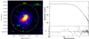 |
Fig. 1. Left: MACS J1149 X-ray map obtained with Chandra in the 0.5–3 keV band (1 pix = 4″). The region within R500 is indicated in yellow and cyan circles label the location of the three sub-clusters, as reported by Golovich et al. (2016). The cluster is elongated along NW-SE. Sub-cluster 1 is associated with the main X-ray concentration, whereas no clumps associated with sub-cluster 2 are clearly visible. Right: X-ray surface brightness profile. Data are fitted by a β-model (blue line) with β = 0.66 ± 0.01 and rc = 288 ± 8 kpc. |
As shown by deep Chandra X-ray observations (Ogrean et al. 2016), the ICM has a globally high temperature of kT ∼ 10 keV and is elongated along the NW-SE axis, although the main X-ray concentration is associated with the most massive NW sub-cluster only. The presence of many massive components, the elongated morphology, and the absence of a central cool core concentration are indications of a disturbed state of the cluster. This is further confirmed by the concentration (c = 0.120 ± 0.003) and centroid-shift (w = 0.017 ± 0.001) parameters estimated by Yuan & Han (2020); these morphological parameters locate MACS J1149 among the disturbed clusters in the c − w bimodal distribution reported by Cassano et al. (2010b). Ogrean et al. (2016) also report the presence of an X-ray surface brightness discontinuity, likely being a cold front, located in the N-NE part of the cluster.
In the radio band, by using VLA and GMRT data, Bonafede et al. (2012) find evidence of diffuse emission, with two possible misaligned relics at south-east and west, and a candidate steep spectrum halo, with α ∼ 2, in line with the complex dynamics of the system. During the preparation of this work, Giovannini et al. (2020) first presented some of the new JVLA observations of the cluster that we used in our analysis (see Sect. 3.4 for details). These authors revise the nature of the candidate west relic, classify it as a radio galaxy, and suggest that the south-east relic might be instead a filamentary structure, whose major axis is parallel to the merger axis. Throughout the paper, we refer to the SE source as the ‘relic’, following the original classification proposed by Bonafede et al. (2012).
3. Observations and data reduction
In this section we present the X-ray and radio data, summarised in Tables 1 and 2, respectively, and briefly describe the reduction processes.
Details of the Chandra X-ray data analysed in this work (PI: C. Jones).
Details of the LOFAR (LoTSS, pointing name: P177+22), GMRT (PI: M. Brüggen, project code: 20_066), and JVLA (PI: A. Bonafede, project code: 13A-056; PI: R. J. van Weeren, project code: 14B-205) radio data analysed in this work.
3.1. Chandra X-ray data
We analysed archival Chandra X-ray data (first presented by Ogrean et al. 2016) of MACS J1149, observed in VFAINT mode with ACIS-I. We reprocessed the six considered observations using CIAO v. 4.12, with CALDB v. 4.9.0. We extracted light curves from the S2 chip (when available) or from one of the I-chips (free of the target emission) in order to filter out soft proton flares with the lc − clean algorithm, which left 287.8 ks of total clean time.
We combined each point spread function (PSF) and the exposure maps to produce a single exposure-corrected PSF map. This map was used as input in the wavdetect task to find point sources, which we then inspected by eye. Spurious sources were excluded and the confirmed sources were excised.
The X-ray analysis of galaxy clusters requires a careful treatment of the background, which has various origins: the local hot bubble (LHB), the galactic halo (GH), the unresolved X-ray sources (CXB), and the particle background (NXB). In particular, we modelled the LHB and the GH with a single absorbed thermal plasma (APEC model) of kT = 0.20 keV, and the CXB with an absorbed power-law of photon index Γ = 1.45; the NXB was obtained by fitting the single spectra extracted from the reprojected stowed background observations and combining a power-law, a decaying exponential, and a number of Gaussian profile lines (as described in Bartalucci et al. 2014). To model the sky components, we extracted the spectra from the observations in the same regions free of ICM emission and we jointly fitted these with the XSPEC v. 12.10.1 package (Arnaud et al. 1996) in the 0.7–11.0 keV band. The NXB emission parameters were kept fixed as obtained by the fit of the single observations. We adopted the Cash statistics (Cstat; Cash 1979) and fixed the (atomic + molecular) hydrogen column density in the direction of the cluster to nH = 2.06 × 1020 cm−2 (Willingale et al. 2013). In the following, errors on fitted parameters are quoted at the 68% confidence level.
3.2. LOFAR radio data
Observations of the LOFAR Two-meter Sky Survey (LoTSS; Shimwell et al. 2017, 2019) are particularly suitable for the detection of extended and low brightness diffuse emission with steep spectrum, such as radio halos and radio relics. MACS J1149 is located at 21 arcmin from the centre of the LoTSS pointing P177+22, which was observed for 8 h on 4 May 2017 using the High Band Antennas (HBA) Dutch array operating in the 120–168 MHz frequency range. The source 3C 295 was used as flux density scale calibrator.
Data were processed by means of the LOFAR Surveys Key Science Project reduction pipeline v2.23 (Shimwell et al. 2019; Tasse et al. 2021), which performs both direction-independent and direction-dependent calibration using PREFACTOR (Offringa et al. 2013; van Weeren et al. 2016; Williams et al. 2016; de Gasperin et al. 2019) and KillMS (Tasse 2014a,b; Smirnov & Tasse 2015) and delivers images at 6″ and 20″ resolution of the full LOFAR field of view using DDFacet (Tasse et al. 2018). In order to improve the image quality towards MACS J1149, we used the models produced by the pipeline to subtract the sources outside a region of sizes 27′ × 27′ centred on the target from the uv data. We used this ‘extracted’ dataset to perform additional cycles of amplitude and phase self-calibration (see details in van Weeren et al. 2020) using WSClean v. 2.7 (Offringa et al. 2014; Offringa & Smirnov 2017). We then checked for possible systematics in the flux density scale by comparing compact discrete sources in the field with the TIFR GMRT Sky Survey Alternative Data Release (TGSS-ADR; Intema et al. 2017), finding no significant offset; typical offsets are of the order of 3%, where one source has a 10% offset.
3.3. GMRT radio data
We retrieved archival GMRT data (first presented by Bonafede et al. 2012) in the 305–340 MHz band, for a total bandwidth of 32 MHz, split into 256 channels. Two observations of 1 and 4 h on-source time are available, and the sources 3C286 and 3C147 were used as absolute flux density scale calibrators. We reprocessed these observations independently via the Source Peeling and Atmospheric Modeling (SPAM) automated pipeline (Intema et al. 2009), which corrects for ionospheric effects and removes direction-dependent gain errors, thereby improving the noise and fidelity of the images. Strong sources in the field of view were used to derive directional-dependent gains and fit a phase-screen over the entire field of view. Finally, images were corrected for the system temperature variations between the calibrator and the target.
During the imaging steps, we noticed that the flux density of the point sources in the field were different for the two observations, independent of the adopted primary calibrator. We measured their flux density at 144 (LOFAR), 610 (GMRT), 1500 (JVLA, L band), and 2800 (JVLA, S band) MHz (see notes in Table 2) to check for the spectra of the sources. The expected power-laws are well fitted in the case of the shallower GMRT data, whereas the deeper data appear to be systematically biased low. The logs of the 4 h observation report of high wind speeds, which could have affected some scans and system gains. To account for this problem, we corrected the deeper images by multiplying them for a factor of 1.23, that is the mean ratio of the source flux densities in the shallow and deep maps.
3.4. JVLA radio data
MACS J1149 was observed with the JVLA at 1–2 GHz (L band) in B, C, and D configurations, for 5.5, 2.5, and 1.5 hours on-source time, respectively (see Table 2 for details), with 3C286 as flux density calibrator and J1150+2417 as phase calibrator. The data were recorded with 16 spectral windows, each divided into 64 channels. It is worth mentioning that, during the preparation of this work, data collected in 2013 (except for the observation in D array of 4 March) were published first by Giovannini et al. (2020). Data reduction was carried out with the National Radio Astronomy Observatory (NRAO) Common Astronomy Software Applications (CASA; McMullin et al. 2007) v. 4.7. We removed radio frequency interference (RFI) by means of the AOFlagger software (Offringa 2010; Offringa et al. 2012). The data from B, C, and D configurations were calibrated independently, by performing the standard calibration procedure, which includes the initial phase, bandpass, and gain calibrations. In addition, we performed two rounds of phase-only self-calibration and two rounds of amplitude and phase self-calibration on the individual datasets. Finally, we combined the B, C, and D configuration data to create deep images.
3.5. Radio imaging and source subtraction
The imaging process was carried out for all the datasets with WSClean v. 2.7, which is designed for wide-field, multi-frequency, and multi-scale synthesis. All images are corrected for the primary beam attenuation. For each dataset, we produced maps with different baseline weightings to study the radio emission of the target on various spatial scales. Short baselines are sensitive to the extended emission, whereas long baselines provide a higher resolution. A compromise between sensitivity and resolution can be reached with the robust parameter intermediate weighting (Briggs 1995) and a tapering of the baselines.
The weighting schemes adopted for the maps discussed in the next sections are summarised in Table 3. To properly image the diffuse emission and consistently compare the LOFAR, GMRT, and JVLA (D array) maps, we adopted a common minimum baseline of 170λ (which gives a maximum recoverable scale of ∼20′, corresponding to ∼8 Mpc), a Briggs weighting with robust 0, and a tapering of the long baselines (10″). We then smoothed these maps with a 30″ × 30″ beam. In addition, we produced an intermediate resolution (19″ × 15″) LOFAR map, which we used for subsequent analysis (see Sects. 4.4 and 5.1).
Summary of the parameters adopted to produce the radio maps discussed in the paper.
We have to remove the contribution of the sources embedded in the halo to measure its flux density. For LOFAR and GMRT datasets, we selected the sources by imaging the data at high resolution, excluding the shortest baselines (< 4kλ; corresponding to maximum angular scales of ∼50″), then we subtracted the clean components in the model image from the uv data. We tested the consistency of this process by comparing the flux density of the halo with that obtained by algebraically subtracting the flux density of the embedded sources from the total (halo plus sources) flux density, finding a good agreement (within 3% and 5% of the flux density for LOFAR and GMRT, respectively). Subtracting the clean components of the discrete sources is not sufficiently accurate with the JVLA datasets, given the very low flux density of the halo. The low sensitivity to extended sources of the B array and the insufficient depth of the C array data, do not allow us to accurately recover the halo emission. On the other hand, the low resolution of the D array makes it difficult to obtain a good model of both point and extended sources. However, we can use the sensitive high-resolution images to identify faint compact sources in the halo region, which contribute to the total flux density when measured from lower resolution images. Therefore, we accurately measured the flux density of point sources in B and C configurations at high resolution, the extended sources in D configuration at low resolution, and then we subtracted their contribution out of the total (halo plus sources) flux density obtained in D array. The model subtraction from the uv data bias the net flux density of the halo at 1.5 GHz high, but the algebraic subtraction might bias the net flux density low; to take into account this effect, we safely considered the 20% of the flux density as the uncertainty on the subtraction.
In the following, the position angle (P.A.) of the beam is measured north-eastwards. The uncertainties ΔS on the reported flux densities are given by
 (1)
(1)
where σ is the RMS noise of the map, Nbeam is the number of independent beams within the considered region, ξcal is the calibration error, and ξsub is the uncertainty of the source subtraction. As mentioned, we assumed ξsub = 3%, 5%, and 20% for LOFAR, GMRT, and JVLA, respectively. We adopted ξcal = 10% for LOFAR (which is lower than the 20% reported in Shimwell et al. 2019, given the low-significance offset found with respect to the TGSS image), ξcal = 10% for GMRT (Chandra et al. 2004), and ξcal = 5% for JVLA (Perley & Butler 2013).
4. Results
In this section we first show the results of the X-ray and radio data analysis, then we investigate the connection between the thermal and non-thermal emission.
4.1. Global X-ray properties
In Fig. 1 (left) we present the exposure-corrected map of MACS J1149 in the 0.5–3 keV band, obtained by merging the six Chandra observations listed in Table 1. The cyan circles indicate the locations of the three sub-clusters, as reported by Golovich et al. (2016); they have virial masses of M1 ∼ M2 ∼ 1015 M⊙, M3 ∼ 1014 M⊙, respectively. The ICM appears elongated along the NW-SE axis, where sub-clusters 1 and 2 lie. Even though sub-clusters 1 and 2 have similar masses, only the most massive sub-cluster 1 is associated with the main X-ray concentration; the depth of the data would be sufficient to detect X-ray clumps associated with sub-cluster 2, if any.
In the right panel of Fig. 1 we show the surface brightness profile within a circle (centred on the pixel coincident with the X-ray peak) of radius R500 = 1.6 Mpc, extracted and fitted by means of the PROFFIT v. 1.5 code (Eckert et al. 2011). The background was assumed to be constant. It was estimated in a source-free region and subtracted, whereas the data were fitted with a simple beta profile under the assumptions of a isothermal gas and a spherical geometry (Cavaliere & Fusco-Femiano 1976) as follows:
![Mathematical equation: $$ \begin{aligned} n_{\rm th}(r)=n_{\rm th,0}\left[1+\left(\frac{r}{r_{\rm c}}\right)^2 \right]^{-\frac{3}{2}\beta }, \end{aligned} $$](/articles/aa/full_html/2021/06/aa39877-20/aa39877-20-eq3.gif) (2)
(2)
where nth is the thermal particle density number, rc is the core radius, and the index β represents the ratio of the kinetic energy of the galaxies to the thermal energy of the gas. The thermal particle distribution is related to the X-ray surface brightness profile IX(r) as (Sarazin 1986)
![Mathematical equation: $$ \begin{aligned} I_{\rm X}(r)=\sqrt{\pi }n_{\rm th,0}^2r_{\rm c}\Lambda (T)\frac{\Gamma (3\beta -0.5)}{\Gamma (3\beta )}\left[1+\left(\frac{r}{r_{\rm c}}\right)^2 \right]^{\frac{1}{2}-3\beta }, \end{aligned} $$](/articles/aa/full_html/2021/06/aa39877-20/aa39877-20-eq4.gif) (3)
(3)
where  is the cooling function in the case of a plasma at a temperature T emitting through thermal bremsstrahlung (e.g., Gitti et al. 2012). The beta model has commonly been used to describe the radial profile of a number of galaxy clusters, providing reasonable representations of the data (Arnaud 2009) even with χ2/d.o.f. ∼ 2 (see e.g., Table 5 reported in Eckert et al. 2011). We obtained β = 0.66 ± 0.01 and rc = 288 ± 8 kpc, where χ2/d.o.f. = 2.3, which is consistent with the typical values found for merging clusters (Forman et al. 1984).
Finally, the X-ray spectrum extracted within R500 is shown in Fig. 2; we jointly fitted all the observations, but we report only one spectrum to avoid confusion in the plot. The particle and sky background components were modelled as described in Sect. 3.1, whereas we adopted an absorbed APEC for the ICM emission. We obtained a global temperature of kT = 10.5 ± 0.3 keV and a metallicity of Z = 0.23 ± 0.05 Z⊙ (Cstat/d.o.f. = 3530/3076). The computed flux within R500 is ![Mathematical equation: $ F_\mathrm{ [0.1{-}2.4 \; keV]}^{500}=(1.67\pm0.01)\times10^{-12} \; \mathrm{erg \; s^{-1} \; cm^{-2}} $](/articles/aa/full_html/2021/06/aa39877-20/aa39877-20-eq6.gif) , which gives a luminosity of
, which gives a luminosity of ![Mathematical equation: $ L_\mathrm{ [0.1-2.4 \; keV]}^{500}=(1.35\pm0.01)\times10^{45} \; \mathrm{erg \; s^{-1}} $](/articles/aa/full_html/2021/06/aa39877-20/aa39877-20-eq7.gif) , in agreement with the values reported by Ogrean et al. (2016).
, in agreement with the values reported by Ogrean et al. (2016).
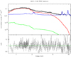 |
Fig. 2. MACS J1149 X-ray spectrum within R500. Data and best-fit model are shown in black. The red, green, and blue curves indicate the cluster emission, the sky background, and the NXB, respectively. The bottom panel shows the ratio of the data to the model. Fits were performed simultaneously for all the observations, but we report only one spectrum for a clearer inspection of the plot; kT = 10.5 ± 0.3 keV and Z = 0.23 ± 0.05 Z⊙ were obtained. |
4.2. Surface brightness edges
We searched for possible substructures in the X-ray surface brightness distribution. As a first step, we used the CONTBIN v. 1.6 code (Sanders 2006) to adaptively bin the surface brightness map into regions with a signal-to-noise ratio of S/N = 30, thus ensuring enough source and background counts. Then, we extracted the spectra within those regions and jointly fitted them, such that the background and metallicity were kept fixed to the previously obtained values, to produce the temperature map shown in Fig. 3; the error map on the right was obtained as the mean of the lower and upper errors. As a general trend, we note that the eastern regions of the cluster are colder than the western regions; this is also visible in the temperature map shown in Ogrean et al. (2016) and obtained with a lower S/N = 10. Moreover, we observe a difference in temperature northwards and southwards with respect to the global value, but the error map indicates that only the northern region has a temperature significantly different (kT = 7.2 ± 0.6 keV) from that of the surrounding bins.
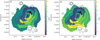 |
Fig. 3. Temperature (left) and associated error (right) maps, reported in keV units. The X-ray surface brightness contours of Fig. 1 are reported in black. The temperature map suggests the presence of a significant lower kT region in NW. |
Discontinuities and substructures in the surface brightness profile can be enhanced by means of the Gaussian gradient magnitude (GGM; Sanders et al. 2016a,b) filtering. We tested different σGGM scales (i.e. the width of the derivative of the Gaussian curve): too narrow scales (< 4″) are usually not efficient in detecting edges in the outskirts of the cluster, owing to the low counts, whereas too large scales (> 8″) could give excessively smoothed images (e.g., Botteon et al. 2018). We found that possible discontinuities are better highlighted with σGGM = 1, 2 pixels, where 1 pixel correspond to 4″ in our maps.
In Fig. 4 (top panel) we show the GGM-filtered image with σGGM = 1 pix. This map reveals two distinct possible edges in the NE and NW, instead of the single one reported by Ogrean et al. (2016), which partially covers both of the edges. In particular, the candidate NW edge is coincident with the cold region highlighted by the temperature map. We do not find discontinuities in the south, however we confirm the presence of two filamentary structures, as found with the unsharp mask analysis by Ogrean et al. (2016), who referred to these structures as the X-ray tail (SW) and peak (SE). The GGM-filtering suggests that they could both be tails, likely associated with the cluster dynamics.
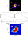 |
Fig. 4. Top: GGM-filtered X-ray image with σGGM = 4″. Two possible surface brightness edges are revealed in the NE and NW. Two filamentary structures (the ‘tails’) are present at south. Middle left: best fit (χ2/d.o.f. = 0.99) of the NE edge with a broken power law. The density compression factor is C = 1.38 ± 0.11. Middle right: best fit (χ2/d.o.f. = 1.12) of the NW edge with a broken power law. The density compression factor is C = 1.52 ± 0.11. A fit with a single power law is rejected (χ2/d.o.f. = 1.80) and thus not shown. Bottom: X-ray count image showing the sectors used to extract the spectra upstream and downstream the surface brightness discontinuities. There are no significant temperature jumps. |
We extracted the surface brightness profiles in the purple and green sectors to study the two candidate discontinuities. We fitted these discontinuities with a broken power-law model (e.g., Owers et al. 2009) as follows:
 (4)
(4)
where C is the density compression factor, a and b are the power-law slopes, and RD is the radius of the edge. The fitted profiles are shown in Fig. 4 (middle panels) and the obtained values are summarised in Table 4. The two discontinuities give similar compression factors, where C = 1.38 ± 0.11 for the NE, and C = 1.52 ± 0.11 for the NW. The NE edge is less prominent than the NW edge and we also tested a single power-law model. The resulting χ2/d.o.f. of the fits are 0.99 and 1.80 with the broken power-law and the single power-law, respectively, thus we rejected the latter case.
The nature of the edges can be investigated by the sign of the jump in temperature. Therefore, we extracted the spectra in inner (downstream) and outer (upstream) sectors, with respect to the radii of the jumps (see Fig. 4, bottom). We did not find clear indications of temperature discontinuities: we obtained  keV and
  keV for the NE edge, and
  keV and
  keV for the NW edge (see Table 4).
Under the assumption of a shock moving outwards from the cluster centre, the Hugoniot-Rankine density jump condition for a mono-atomic thermal gas can be used to compute the corresponding Mach number
 (5)
(5)
The associated temperature jump is given by:
 (6)
(6)
Equation (5) provides Mach numbers of ℳNE = 1.26 ± 0.08 and ℳNW = 1.36 ± 0.08, implying temperature jumps of (Tin/Tout)NE = 1.25 ± 0.07 and (Tin/Tout)NW = 1.35 ± 0.08. In the most favourable scenario, by assuming the upper limits for the downstream temperatures (i.e. kTin, NE = 10.7 keV and kTin, NW = 10.0 keV), the corresponding upstream temperatures from Eq. (6) would result in kTout, NE = 8.6 ± 0.5 keV and kTout, NW = 7.4 ± 0.4 keV. We fixed these temperatures and re-fitted the spectra, but the Cstat increases (ΔCstatNE = 1.9, ΔCstatNW = 4.4). Lower downstream temperatures would result in even worse fit, thus we conclude that the edges are unlikely to be shock fronts.
The two discontinuities may be associated with cold fronts. The N-NE edge revealed by Ogrean et al. (2016) was classified as a candidate cold front, which would be one of the most distant cold fronts to date, if confirmed. This N-NE edge is roughly located in the middle between the NE and NW edges we found and has a compression factor consistent with ours. Even though GGM filtering is efficient in separating the discontinuities, the low source counts in the upstream sectors do not allow us to confirm whether the NE and NW can be considered a single or double edge; in this regard, projection effects may play an important role. That said, we note that the temperature map in Fig. 3 suggests similarities with the prototypical case of Abell 3667 (Owers et al. 2009; Ichinohe et al. 2017), where the coolest gas of the system is pushed at the tip of the cold front surrounded by the hotter gas. This interpretation would be in line with the merger scenario described by Golovich et al. (2016) between sub-cluster 1 and sub-cluster 2.
4.3. Radio maps and properties
In the left panel of Fig. 5 we present our 144 MHz LOFAR map at 10″ × 6″ resolution, while the right panel reports the 1.5 GHz JVLA map at 5″ × 4″ resolution obtained by combining the data in B, C, and D arrays. These high-resolution images show the presence of several compact and extended sources.
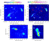 |
Fig. 5. MACS J1149 radio maps at high resolution. In all the panels, the white contour levels are [ ± 3, 6, 12, …]×σ. The dashed yellow contour indicates the 3σ (with σ ∼ 0.30 mJy beam−1) level of the 30″ × 30″ resolution LOFAR map after the subtraction of the embedded sources (see also Fig. 6). Top left: 144 MHz LOFAR map at 10″ × 6″ resolution (P.A. = 81° , σ ∼ 0.15 mJy beam−1). The western source ‘L’ has recently been reclassified as a radio galaxy. The SE relic is labelled as ‘J’ and a bridge-like structure links it to the source ‘K’. Top right: 1.5 GHz JVLA (B, C, D arrays combined) map at 5″ × 4″ resolution (P.A. = 16o, σ ∼ 18 μJy beam−1) showing the discrete sources embedded in the radio halo. Bottom left: zoom of the above LOFAR image on the two extended sources ‘B’ (head-tail radio galaxy) and ‘C’. Bottom right: zoom of the above JVLA image on the radio galaxy ‘L’ showing its FRI morphology. |
The bright elongated sources in the south-east (‘J’) and west (‘L’) are the relic and the candidate relic, respectively, reported by Bonafede et al. (2012); these sources are well recovered at both frequencies. As mentioned, the source ‘L’ has been recently reclassified as a radio galaxy (Giovannini et al. 2020). This is further confirmed by means of our deeper JVLA data: the bottom right panel of Fig. 5 focusses on the source ‘L’ and unambiguously indicates that it is a radio galaxy that has a well-resolved core and jets, no hotspots, and has a FRI (Fanaroff & Riley 1974) morphology. We measured a flux density of S144 = 63.8 ± 6.4 mJy, S323 = 39.9 ± 4.1 mJy, and S1500 = 17.2 ± 0.9 mJy at 144, 323, and 1500 MHz, respectively. We fitted these values with a single power-law, obtaining a spectral index  between 144 and 1500 MHz, which is consistent with the typical spectra of radio galaxies. We note that the flux density measured by Giovannini et al. (2020) at 1.5 GHz is significantly lower (by a factor ∼2); their maps are shallower (the RMS is ∼2 times higher) than ours and allow these authors to recover only the brightest inner emission of the source (roughly corresponding to the 12σ level in the bottom right panel of Fig. 5).
The halo emission is not clearly detected at the 3σ level, owing to its low surface brightness and the high resolution of the images. There are two extended sources, ‘B’ and ‘C’, highlighted in the bottom left panel. An accurate description of the SE relic ‘J’ is beyond the scope of this work, however we notice that the source ‘K’ at its SW appears to be partially embedded in diffuse emission and shows an interesting bridge-like structure linking ‘K’ with the SE relic. As a result of their shallower data, this bridge is not detected by Giovannini et al. (2020). It is not clear whether this diffuse emission belongs to the relic or the source itself. As discussed by Giovannini et al. (2020), the orientation of ‘J’ is expected to be perpendicular to the merger axis if it is a relic induced by the merger shock. Therefore, they proposed that ‘J’ might be a radio filament associated with the merger and not a relic.
Figure 6 shows the 30″ × 30″ resolution maps at 144 MHz (top left), 323 MHz (top right), and 1.5 GHz (bottom left), which we used to consistently measure the flux density of the halo. For the first time, we have deep radio maps of the halo at high and low frequency and a more reliable measure of the spectrum can be performed. In all these images, the diffuse emission extends up to ∼400″ (∼2.6 Mpc) along the NW-SE direction, even though it is fully recovered only at 144 MHz. The morphology of the halo emission is similar at 144 MHz, 323 MHz, and 1.5 GHz. It has a projected NW-SE length of ∼200″ (∼1.3 Mpc) and is interconnected with the relic. In the bottom right panel of Fig. 6 we overlay the LOFAR contours (after the subtraction of the sources embedded in the halo) on the X-ray image of Fig. 1. The radio emission of the halo is co-spatial with the X-ray emission of the ICM, as typically observed in galaxy clusters.
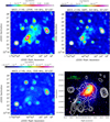 |
Fig. 6. MACS J1149 radio maps at 30″ × 30″ resolution. In all the panels, the contour levels are [ ± 3, 6, 12, …]×σ. Top left: 144 MHz LOFAR map (σ ∼ 0.30 mJy beam−1). Top right: 323 MHz GMRT map (σ ∼ 0.30 mJy beam−1). Bottom left: 1.5 GHz JVLA (D array) map (σ ∼ 45 μJy beam−1). Bottom right: 144 MHz LOFAR contours (after the subtraction of the embedded sources) overlaid on the X-ray image of Fig. 1. |
A number of compact sources, labelled in Fig. 5, and the above-mentioned ‘B’ and ‘C’ sources are embedded within the halo. In particular, source ‘B’ at 144 MHz apparently has a head-tail morphology; the tail is barely visible above 323 MHz. Source ‘C’ lies in the centre of the halo and appears extended. In Fig. 7 we overlay the high-resolution LOFAR contours on the RVB-filters image of the cluster obtained with Subaru/Suprime-Cam (Miyazaki et al. 2002). This image suggests a possible association of the source ‘C’ with a cluster member galaxy (coordinates RAJ2000 11h49m35.51s, DecJ2000 22° 24′03.76″).
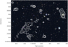 |
Fig. 7. Japanese Virtual Observatory Subaru (RVB filters) image of MACS J1149. The contours of the 144 MHz LOFAR map (10″ × 6″, P.A. = 81°) shown in Fig. 5 are shown in white. |
As discussed in Sect. 3.5, the approaches of subtracting the visibilities and the flux densities of the sources are consistent in the LOFAR and GMRT datasets. However, given the very low flux density of the halo at 1500 MHz, small errors in the subtraction may bias it high, and given the JVLA image properties we have more confidence in the algebraic subtraction. Table 5 summarises the net flux density of the halo and the embedded sources (we also report the source ‘L’). The obtained values of the halo within the 3σ LOFAR contours (by avoiding contamination of the regions nearby the relic4) are S144 = 65.8 ± 7.1 mJy, S323 = 19.4 ± 3.1 mJy, and S1500 = 2.0 ± 0.5 mJy, respectively. The resulting spectrum across 144 and 1500 MHz is reported in Fig. 8. We fitted the flux density values with a single power-law, obtaining a spectral index of  . We iterated the measures in different regions of the halo (in particular, within the brightest X-ray counterpart; see Fig. 6, bottom right), consistently finding an average α ∼ 1.5 everywhere and thus confirming that MACS J1149 is a steep spectrum radio halo. We note that Bonafede et al. (2012) measure S323 = 29 ± 4 mJy and S1500 = 1.2 ± 0.5 mJy (
 ), whereas Giovannini et al. (2020) obtained S1500 = 0.9 ± 0.1 mJy. The inconsistency of these values with our measure at 1.5 GHz derives from the fact that our observations includes D array data that are deeper and more sensitive to the extended emission, thus allowing us to properly recover the emission of the halo at high frequency and providing a more reliable measure of the total flux density; the higher flux density at 323 MHz reported by Bonafede et al. (2012) is likely due to the different adopted weighting scheme and a larger considered area that might be contaminated by the SE relic.
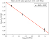 |
Fig. 8. Radio spectrum of the halo between 144 and 1500 MHz (see Table 5). The solid line indicates the fitted power-law. The resulting spectral index is |

By using the flux density and the fitted spectral index, we computed the corresponding radio powers as
 (7)
(7)
We obtained P144 = (9.3 ± 1.0)×1025 W Hz−1, P323 = (2.7 ± 0.5)×1025 W Hz−1, and P1500 = (2.8 ± 0.7)×1024 W Hz−1, at 144, 323, and 1500 MHz, respectively. Radio halos with steep spectrum are found to be radio under-luminous with respect to the correlation reported by Cassano et al. (2013) between the 1.4 GHz radio power and mass of the host cluster. By extrapolating from the radio spectrum, the flux density at 1.4 GHz results S1400 = 2.2 ± 0.6 mJy, and we calculated a power of P1400 = (3.1 ± 0.9)×1024 W Hz−1. Indeed, MACS J1149 as well falls below this correlation by a factor of ∼3, as shown with a red dot in Fig. 9.
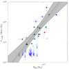 |
Fig. 9. Distribution of galaxy clusters in the P1400 − M500 plane (adapted from Cassano et al. 2013, see it for details of the legend). MACS J1149 (red dot) has M500 = (10.4 ± 0.5)×1014 M⊙ and P1400 = (3.1 ± 0.9)×1024 W Hz−1; it is under-luminous with respect to the correlation by a factor of ∼3 and is located among the steep spectrum radio halos (green dots). |
4.4. Thermal-non-thermal correlation
As typically found in radio halos, the non-thermal emission in MACS J1149 roughly follows the thermal emission (Fig. 6, bottom right). The left panel of Fig. 10 shows the radio (IR), and X-ray (IX) surface brightness radial profiles, extracted in circular beam-size annuli and normalised at their respective maxima; we used the LOFAR image at 19″ × 15″ resolution. We note that IR decreases with the radius slower than IX.
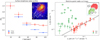 |
Fig. 10. Left: radio (red circles) and X-ray (blue triangles) surface brightness radial profiles within the halo region, normalised at their maximum. The source-subtracted LOFAR map at 19″ × 15″ resolution sampled with concentric annuli of 19″ width is shown in the corner. Right: point-to-point analysis of the IR − IX relation. In the corner, we report the contours of the 30″ × 30″ source-subtracted LOFAR map, gridded with green and red 30″ × 30″ square boxes for the relic and halo, respectively. The halo points present a sub-linear correlation with a slope in the range [0.42–0.60]. The black line represents the best fit obtained with the BCES-orthogonal method at 3σ threshold. |
A point-to-point correlation of the type of  between the radio and X-ray surface brightness is found for a number of radio halos (e.g., Feretti et al. 2001; Govoni et al. 2001; Giacintucci et al. 2005; Hoang et al. 2019; Botteon et al. 2020b; Xie et al. 2020), which have typical sub-linear slopes k < 1, meaning that IR increases slower than IX. We investigated this relation in MACS J1149 by means of the code described in Ignesti et al. (2020). The code allows us to sample an extended radio source down to a given threshold in surface brightness by gridding it with square cells. Both IR and IX are measured within each cell, then the data are fitted with a power-law and the Pearson (ρp) and Spearman (ρs) ranks are computed.
The LOFAR source-subtracted map at resolution 30″ × 30″ was used to grid both the halo and relic with beam-size cells, as represented in the right panel of Fig. 10. The green and red points mark the relic and halo cells, respectively. The plot clearly shows that the halo data follow a tight (ρp = 0.93, ρs = 0.91) correlation, whereas the data extracted from the region of the relic are uncorrelated. Halos and the ICM are thought to share a similar volume, whereas the volume occupied by relics is much lower because, at a first approximation, they can be considered as bi-dimensional sources; therefore a physical correlation is only expected for the halos. Since no correlation seems to exist between the relic and the ICM, this allows us to better discriminate the halo region from that of the relic. Nevertheless, the transition region was excluded to avoid any possible contamination to the fit of the correlation slope.
We explored the correlation strength of the halo through various fitting methods: BCES (Bivariate Correlated Errors and intrinsic Scatter; Akritas & Bershady 1996) bisector and orthogonal, and linmix (Kelly 2007). Moreover, we checked for possible biases due to the choice of the radio brightness threshold. The results are listed in Table 6. There is a good agreement among the three methods, but we notice that the fit is sensitive to the adopted threshold, especially in the case of BCES bisector and orthogonal. Even though the values of k are consistent, lower thresholds give steeper indices, as recently discussed in Botteon et al. (2020b). Anyway, we find that the IR − IX correlation is strongly sub-linear in MACS J1149, where k is in the range [0.42–0.60].
Results from the IR − IX point-to-point analysis of the halo.
5. Discussion
In this section, we discuss the formation process of the halo and its connection with the cluster dynamics.
5.1. Constraining the hadronic contribution
In general, hadronic scenarios are disfavoured by the observed connection between radio halos and the cluster dynamics (e.g., Brunetti & Jones 2014; van Weeren et al. 2019). In a few cases, the spectral properties of the halos (e.g., Brunetti et al. 2008; Wilber et al. 2018) and the limits to the gamma-ray emission of the hosting clusters (Brunetti et al. 2012, 2017; Zandanel & Ando 2014) provide constraints that are sufficiently stringent to allow pure hadronic models to be excluded. The radio halo in MACS J1149 combines a high redshift with a steep radio spectrum (Fig. 8) and a flat radial profile (Fig. 10, left), which overall challenges a hadronic origin. In the following, we show that the properties of MACS J1149 allow us to test hadronic models without using complementary constraints from gamma-rays.
We aim to estimate the non-thermal energy in the cluster required to reproduce the observed radio emission in a pure hadronic scenario. The stationary spectrum of electrons and positrons produced by hadronic collisions in the ICM is (Dolag & Enßlin 2000) given by
 (8)
(8)
where p is the momentum of the particles,  are the radiative and Coulomb losses, and
  is the injection rate of electrons and positrons defined as (Brunetti & Jones 2014, and references therein)
 (9)
(9)
where the pedices ‘π’, ‘μ’, and ‘p’ refer to pions, muons, and protons, respectively,  ,
, ![Mathematical equation: $ \bar{E}_\upmu=\frac{E_\pi}{0.5428}\left[ 1-\left( \frac{m_\upmu}{m_\pi} \right)^2 \right] $](/articles/aa/full_html/2021/06/aa39877-20/aa39877-20-eq36.gif) , and
, and  is the differential inclusive cross-section for the production of π+, π−, and π0 (we assume the cross-section as in Brunetti et al. 2017), and Fe(Ee, Eπ) is defined as in Brunetti & Blasi (2005) (Eqs. (36) and (37)).
We derived the distribution of the thermal protons, nth(r), from the X-ray surface brightness profile IX(r) (index β = 0.66, core radius rc = 288 kpc, and central proton density number nth, 0 = 3.6 × 10⁻³ cm−3; see Eqs. (2) and (3)). We also assume that the magnetic field scales with the thermal proton density as
![Mathematical equation: $$ \begin{aligned} B(r)=B_0 \left[ \frac{n_{\rm th}(r)}{n_{\rm th,0}}\right]^\eta , \end{aligned} $$](/articles/aa/full_html/2021/06/aa39877-20/aa39877-20-eq38.gif) (10)
(10)
where we fixed η = 0.5, which is the value that gives the equilibrium between the thermal and magnetic energy densities (e.g., Bonafede et al. 2010).
The secondary CRe injected in the ICM magnetic field produce synchrotron radio emission with an emissivity given by (Dolag & Enßlin 2000)
 (11)
(11)
where θ is the pitch angle between B and p,  is the synchrotron kernel (Rybicki & Lightman 1979), and BCMB = 3.25(1 + z)2 μG is the CMB equivalent magnetic field. Under the assumption of a spherical geometry, the integral of jR(ν, r) along the line of sight provides the surface brightness profile at a projected distance b as follows:
 (12)
(12)
By assuming a value of the central field B0 and taking into account the effects of the k-correction, we matched the radio profile from Eq. (12) with the observed profile to derive the momentum distribution of CRp in the form (Brunetti & Jones 2014)
 (13)
(13)
where Kp(r) is the normalisation and s = 2α (where α = 1.5, inferred from the radio spectrum of the halo). Thus, the energy budget of the CRp is obtained as
 (14)
(14)
where we consider a minimum momentum of the CRp spectrum of pmin = 0.5mpc, corresponding to a kinetic energy of Emin ∼ 110 MeV.
The ratio of CRp and thermal energy budget required to match the observed radio emission assuming a pure hadronic model is shown in Fig. 11 as a function of B0. We also show the ratio of the thermal (εICM) and non-thermal (εCR + εB) energy budget, integrated within maximum radii of 2.2rc and 2.5rc, where the halo is clearly visible (see Fig. 6). For typical values of B0 < 10 μG in galaxy clusters (e.g., Bonafede et al. 2010), an untenable εCR/εICM > 1 is required. The CRe energy budget declines with increasing B0; however the minimum (εCR+εB)/εICM is reached for unusually high values of the magnetic field B0 ∼ 25 μG. Moreover, the CRe energy budget is still extremely large (∼40−50%). In comparison, the Fermi satellite constrains the CRe energy budget to few percent in Coma and other nearby galaxy clusters (Ackermann et al. 2014; Brunetti et al. 2017).
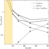 |
Fig. 11. Non-thermal to thermal energy budget as a function of the central magnetic field in a pure hadronic model. The dashed, dotted, and solid lines are the CRe to ICM energy ratio, the magnetic to ICM energy ratio, and the total non-thermal to ICM energy ratio, respectively; these are required to match the observed radio emission up to radii of 2.2rc (lower dashed and solid lines) and 2.5rc (upper dashed and solid lines). The non-thermal energy budget for typical values of B0 ≲ 10 μG in galaxy clusters is indicated by the yellow area. A pure hadronic model would require unrealistically high values of (εCR+εB)/εICM and/or B0. |
Under the assumption of a spherical symmetry of the ICM and CRp distribution, the most important parameter is the minimum energy of CRp. If we conservatively assumed Emin = 300 MeV (i.e. the minimum threshold for CRp-p collisions), εCR would result to be 30% smaller than in Fig. 11; on the other hand, extending the CRp spectrum at lower energies down to Emin = 20 keV and Emin = 1 MeV would boost up εCR by a factor of 3.4 and 2.3, respectively. For these reasons, we can rule out an hadronic origin of the halo; by considering εCR/εICM to be few percent, CRe would contribute to < 10% of the halo emission. Nevertheless, we cannot exclude that hadronic collisions still play a role by injecting secondary particles that are eventually re-accelerated by turbulence (Brunetti & Lazarian 2011; Pinzke et al. 2017).
5.2. Merger scenario
Lensing and spectroscopy studies concluded that MACS J1149 consists of at least three main sub-clusters (Smith et al. 2009; Golovich et al. 2016), whose locations are indicated by open circles in Fig. 1. Sub-clusters 1 and 2 are the most massive; they have virial masses of M1 ∼ M2 ∼ 1015 M⊙, whereas sub-cluster 3 is one order of magnitude less massive M3 ∼ 1014 M⊙.
The ICM has a clearly elongated structure along the NW-SE axis and although sub-clusters 1 and 2 have similar masses, only the first is associated with the main X-ray concentration. According to the scenario proposed by Golovich et al. (2016), a major merger between sub-clusters 1 and 2 occurred ∼1 Gyr ago along the NW-SE direction in the plane of the sky and sub-cluster 2 was stripped of its gas. The two X-ray tails of Fig. 4 in the south could be related to this event. Besides the major merger between sub-clusters 1 and 2, a minor merger between sub-clusters 1 and 3 has begun ∼100 Myr ago, likely along the line of sight (Golovich et al. 2019). Given the high mass ratio, this interaction does not significantly affect the ICM and the major merger dynamics.
In proximity of the N-NE candidate cold front identified by Ogrean et al. (2016), we find instead that there may be two distinct X-ray surface brightness discontinuities in NE and NW, which are possibly cold fronts. However, the case of Abell 3667 (Owers et al. 2009; Ichinohe et al. 2017) suggests a simpler scenario in which we are observing a single cold front, where the coolest gas was pushed towards the NW and is surrounded by the hotter gas. Under this assumption, our cold front can likely be explained with the major merger described above, and its origin could be associated with the cool core of a sub-cluster. However, because of the low count statistic in the upstream regions, at present we cannot disentangle the nature of the discontinuities.
The major merger likely induced the formation of the relic and the halo through shocks and turbulence. Finding that the candidate misaligned W relic is a FRI radio galaxy is in line with this scenario. The steepening of the spectral index of the SE relic towards the centre of the cluster (Bonafede et al. 2012) would also be consistent with this model, however its orientation is peculiar, as it is parallel to the merger axis and not perpendicular, as observed for relic sources. The interaction of a merger shock with remnants or clouds filled by pre-existing relativistic electrons may explain this feature. On the other hand, Giovannini et al. (2020) suggested that the SE source might be a radio filament associated with the halo. Nevertheless, with our data we do not exclude the possibility that the SE source might be a radio galaxy; this will be the subject of a future paper.
Steep spectrum radio halos are predicted as a result of less efficient turbulent acceleration or stronger energy losses (e.g., Brunetti et al. 2008; Cassano et al. 2010b). The former case may result from a less energetic sequence of merger events (e.g., Cassano et al. 2006) or may mark the final evolution phase of energetic mergers where a significant fraction of the turbulence has already been dissipated (Donnert et al. 2013). In both cases, halos are predicted to be under-luminous. The old major merger in MACS J1149 may be in line with the advanced evolution phase scenario, however it is difficult to discriminate between the two possibilities.
6. Summary and conclusions
In this work, we constrained the spectrum of the radio halo in the high-redshift (z = 0.544) MACS J1149 galaxy cluster, by means of multi-frequency LOFAR, GMRT, and JVLA radio data at 144, 323, and 1500 MHz, and found it to be steep. In addition, we used Chandra X-ray data to compare the thermal and non-thermal emission of the target.
MACS J1149 is a merging system consisting of at least three sub-clusters. The X-ray data analysis showed that the ICM is characterised by a remarkably high temperature (kT = 10.5 ± 0.3 keV) and luminosity (![Mathematical equation: $ L^{500}_\mathrm{[0.1{-}2.4 \; keV]}=(1.35\pm0.01)\times10^{45} \; \mathrm{erg\; s^{-1}} $](/articles/aa/full_html/2021/06/aa39877-20/aa39877-20-eq44.gif) ), and is elongated along the NW-SE axis, where the two most massive sub-clusters lie. Despite its large mass, no X-ray clumps are associated with the SE sub-cluster.
), and is elongated along the NW-SE axis, where the two most massive sub-clusters lie. Despite its large mass, no X-ray clumps are associated with the SE sub-cluster.
We found two surface brightness discontinuities, which we interpret as evidence of a temperature gradient within a single cold front, where the coolest gas was pushed towards NW. In this case, the cold front may be explained as the cool core remnant of a sub-cluster involved in the major merger occurred ∼1 Gyr ago. A higher S/N in the upstream regions is required to better constrain the nature of the discontinuities.
We produced radio images at different frequency and resolution, showing that the halo is co-spatial with the ICM. The measured flux densities provide a spectral index  between 144 and 1500 MHz. The computed radio powers of the halo are P144 = (9.3 ± 1.0)×1025 W Hz−1, P323 = (2.7 ± 0.4)×1025 W Hz−1, and P1500 = (2.8 ± 0.7)×1024 W Hz−1. As typical steep spectrum halos, MACS J1149 is under-luminous (by a factor of ∼3) with respect to the correlation found by Cassano et al. (2013) between the 1.4 GHz radio power versus the mass of the cluster.
A point-to-point comparison of the radio and X-ray surface brightness showed a tight sub-linear correlation  , which we investigated through various fitting methods and radio thresholds; we consistently found a slope k in the range [0.42–0.60].
Finally, owing to the high redshift of the cluster, the steep spectrum of the halo, and its flat spatial distribution, we were able to test hadronic models without constraints from gamma-ray observations. Our analysis demonstrated that a significant contribution to the halo from pure hadronic collisions is ruled out. In line with previous studies, the old (∼1 Gyr ago) major merger between the two most massive sub-clusters likely induced turbulence in the ICM, which accelerated particles and formed the halo. The steep spectrum of the halo may results both from low turbulence in combination with high radiative (inverse Compton) losses or an advanced evolution phase.
In addition, we confirm the recent reclassification proposed by Giovannini et al. (2020) of the W source as a radio galaxy, and in particular we point out its FRI morphology. The peculiar orientation of the SE relic may indicate a different nature of this source and requires a more detailed analysis, which is beyond the aim of this work.
We define the spectral index α through S ∝ ν−α, where S is the radio flux density at the frequency ν.
M500 is obtained from R500, which is defined as the radius enclosing 500ρc(z), where ρc(z) is the critical density of the Universe at a given redshift.
The flux density of the halo was measured in a region that roughly corresponds to that sampled with red boxes in Fig. 10, right panel.
Acknowledgments
We thank the referee for his comments and suggestions, that have improved the presentation of the paper. KR acknowledges financial support from the ERC Starting Grant ‘MAGCOW’, no. 714196. GB, FG, and RC acknowledge support from INAF mainstream project ‘Galaxy Clusters Science with LOFAR’, 1.05.01.86.05. A. Botteon acknowledges support from the VIDI research program with project number 639.042.729, which is financed by the Netherlands Organisation for Scientific Research (NWO). AI acknowledges the Italian PRIN-Miur 2017 (PI A. Cimatti). A. Bonafede acknowledges support from the ERC-Stg DRANOEL n. 714245 and from the Italian MIUR grant FARE ‘SMS’. RJvW and GDG acknowledge support from the ERC Starting Grant ClusterWeb, no. 804208. VC acknowledges support from the Alexander von Humboldt Foundation. MB acknowledges support from the Deutsche Forschungsgemeinschaft under Germany’s Excellence Strategy - EXC 2121 “Quantum Universe” – 390833306. LOFAR (van Haarlem et al. 2013) is the Low Frequency Array designed and constructed by ASTRON. It has observing, data processing, and data storage facilities in several countries, which are owned by various parties (each with their own funding sources), and that are collectively operated by the ILT foundation under a joint scientific policy. The ILT resources have benefited from the following recent major funding sources: CNRS-INSU, Observatoire de Paris and Université d’Orléans, France; BMBF, MIWF- NRW, MPG, Germany; Science Foundation Ireland (SFI), Department of Business, Enterprise and Innovation (DBEI), Ireland; NWO, The Netherlands; The Science and Technology Facilities Council, UK; Ministry of Science and Higher Education, Poland; The Istituto Nazionale di Astrofisica (INAF), Italy. This research made use of the Dutch national e-infrastructure with support of the SURF Cooperative (e-infra 180169) and the LOFAR e-infra group. The Jülich LOFAR Long Term Archive and the German LOFAR network are both coordinated and operated by the Jülich Supercomputing Centre (JSC), and computing resources on the supercomputer JUWELS at JSC were provided by the Gauss Centre for Supercomputing e.V. (grant CHTB00) through the John von Neumann Institute for Computing (NIC). This research made use of the University of Hertfordshire high-performance computing facility and the LOFAR-UK computing facility located at the University of Hertfordshire and supported by STFC [ST/P000096/1], and of the Italian LOFAR IT computing infrastructure supported and operated by INAF, and by the Physics Department of Turin University (under an agreement with Consorzio Interuniversitario per la Fisica Spaziale) at the C3S Supercomputing Centre, Italy. The National Radio Astronomy Observatory is a facility of the National Science Foundation operated under cooperative agreement by Associated Universities, Inc. We thank the staff of the GMRT that made these observations possible. GMRT is run by the National Centre for Radio Astrophysics of the Tata Institute of Fundamental Research. The scientific results reported in this article are based on observations made by the Chandra X-ray Observatory data obtained from the Chandra Data Archive. This research has made use of data and/or software provided by the High Energy Astrophysics Science Archive Research Center (HEASARC), which is a service of the Astrophysics Science Division at NASA/GSFC. Based in part on data collected at Subaru Telescope, which is operated by the National Astronomical Observatory of Japan. Part of the data are retrieved from the JVO portal (http://jvo.nao.ac.jp/portal) operated by the NAOJ.
References
- Ackermann, M., Ajello, M., Albert, A., et al. 2014, ApJ, 787, 18 [NASA ADS] [CrossRef] [Google Scholar]
- Ackermann, M., Ajello, M., Albert, A., et al. 2016, ApJ, 819, 149 [NASA ADS] [CrossRef] [Google Scholar]
- Akamatsu, H., Mizuno, M., Ota, N., et al. 2017, A&A, 600, A100 [NASA ADS] [CrossRef] [EDP Sciences] [Google Scholar]
- Akritas, M. G., & Bershady, M. A. 1996, ApJ, 470, 706 [Google Scholar]
- Arnaud, K. A. 1996, in Astronomical Data Analysis Software and Systems V, eds. G. H. Jacoby, & J. Barnes, ASP Conf. Ser., 101, 17 [Google Scholar]
- Arnaud, M. 2009, A&A, 500, 103 [NASA ADS] [CrossRef] [EDP Sciences] [Google Scholar]
- Bartalucci, I., Mazzotta, P., Bourdin, H., & Vikhlinin, A. 2014, A&A, 566, A25 [NASA ADS] [CrossRef] [EDP Sciences] [Google Scholar]
- Beresnyak, A., Xu, H., Li, H., & Schlickeiser, R. 2013, ApJ, 771, 131 [Google Scholar]
- Bîrzan, L., Rafferty, D. A., Cassano, R., et al. 2019, MNRAS, 487, 4775 [NASA ADS] [CrossRef] [Google Scholar]
- Blasi, P., & Colafrancesco, S. 1999, Astropart. Phys., 12, 169 [NASA ADS] [CrossRef] [Google Scholar]
- Bonafede, A., Feretti, L., Murgia, M., et al. 2010, A&A, 513, A30 [NASA ADS] [CrossRef] [EDP Sciences] [Google Scholar]
- Bonafede, A., Brüggen, M., van Weeren, R., et al. 2012, MNRAS, 426, 40 [NASA ADS] [CrossRef] [Google Scholar]
- Bonafede, A., Intema, H. T., Brüggen, M., et al. 2014, ApJ, 785, 1 [NASA ADS] [CrossRef] [Google Scholar]
- Botteon, A., Gastaldello, F., Brunetti, G., & Kale, R. 2016a, MNRAS, 463, 1534 [NASA ADS] [CrossRef] [Google Scholar]
- Botteon, A., Gastaldello, F., Brunetti, G., & Dallacasa, D. 2016b, MNRAS, 460, L84 [NASA ADS] [CrossRef] [Google Scholar]
- Botteon, A., Gastaldello, F., & Brunetti, G. 2018, MNRAS, 476, 5591 [NASA ADS] [CrossRef] [Google Scholar]
- Botteon, A., Brunetti, G., Ryu, D., & Roh, S. 2020a, A&A, 634, [Google Scholar]
- Botteon, A., Brunetti, G., van Weeren, R. J., et al. 2020b, ApJ, 897, 93 [CrossRef] [Google Scholar]
- Bourdin, H., Mazzotta, P., Markevitch, M., Giacintucci, S., & Brunetti, G. 2013, ApJ, 764, 82 [Google Scholar]
- Brentjens, M. A. 2008, A&A, 489, 69 [NASA ADS] [CrossRef] [EDP Sciences] [Google Scholar]
- Briggs, D. S. 1995, in American Astronomical Society Meeting Abstracts, Am. Astron. Soc. Meeting Abstr., 187, 112.02 [Google Scholar]
- Brunetti, G. 2009, A&A, 508, 599 [NASA ADS] [CrossRef] [EDP Sciences] [Google Scholar]
- Brunetti, G., & Blasi, P. 2005, MNRAS, 363, 1173 [Google Scholar]
- Brunetti, G., & Jones, T. W. 2014, Int. J. Mod. Phys. D, 23, 1430007 [Google Scholar]
- Brunetti, G., & Lazarian, A. 2007, MNRAS, 378, 245 [NASA ADS] [CrossRef] [Google Scholar]
- Brunetti, G., & Lazarian, A. 2011, MNRAS, 410, 127 [Google Scholar]
- Brunetti, G., & Lazarian, A. 2016, MNRAS, 458, 2584 [NASA ADS] [CrossRef] [Google Scholar]
- Brunetti, G., Setti, G., Feretti, L., & Giovannini, G. 2001, MNRAS, 320, 365 [NASA ADS] [CrossRef] [Google Scholar]
- Brunetti, G., Giacintucci, S., Cassano, R., et al. 2008, Nature, 455, 944 [NASA ADS] [CrossRef] [Google Scholar]
- Brunetti, G., Blasi, P., Reimer, O., et al. 2012, MNRAS, 426, 956 [NASA ADS] [CrossRef] [Google Scholar]
- Brunetti, G., Zimmer, S., & Zandanel, F. 2017, MNRAS, 472, 1506 [NASA ADS] [CrossRef] [Google Scholar]
- Cash, W. 1979, ApJ, 228, 939 [NASA ADS] [CrossRef] [Google Scholar]
- Cassano, R., Brunetti, G., & Setti, G. 2006, MNRAS, 369, 1577 [Google Scholar]
- Cassano, R., Ettori, S., Giacintucci, S., et al. 2010a, ApJ, 721, L82 [Google Scholar]
- Cassano, R., Brunetti, G., Röttgering, H. J. A., & Brüggen, M. 2010b, A&A, 509, A68 [NASA ADS] [CrossRef] [EDP Sciences] [Google Scholar]
- Cassano, R., Ettori, S., Brunetti, G., et al. 2013, ApJ, 777, 141 [NASA ADS] [CrossRef] [Google Scholar]
- Cavaliere, A., & Fusco-Femiano, R. 1976, A&A, 500, 95 [NASA ADS] [Google Scholar]
- Chandra, P., Ray, A., & Bhatnagar, S. 2004, ApJ, 612, 974 [Google Scholar]
- Cuciti, V., Cassano, R., Brunetti, G., et al. 2015, A&A, 580, A97 [NASA ADS] [CrossRef] [EDP Sciences] [Google Scholar]
- Dallacasa, D., Brunetti, G., Giacintucci, S., et al. 2009, ApJ, 699, 1288 [NASA ADS] [CrossRef] [Google Scholar]
- de Gasperin, F., Dijkema, T. J., Drabent, A., et al. 2019, A&A, 622, A5 [NASA ADS] [CrossRef] [EDP Sciences] [Google Scholar]
- Dennison, B. 1980, ApJ, 239, L93 [NASA ADS] [CrossRef] [Google Scholar]
- Dolag, K., & Enßlin, T. A. 2000, A&A, 362, 151 [NASA ADS] [Google Scholar]
- Donnert, J., Dolag, K., Brunetti, G., & Cassano, R. 2013, MNRAS, 429, 3564 [NASA ADS] [CrossRef] [Google Scholar]
- Ebeling, H., Edge, A. C., & Henry, J. P. 2001, ApJ, 553, 668 [Google Scholar]
- Eckert, D., Molendi, S., & Paltani, S. 2011, A&A, 526, A79 [NASA ADS] [CrossRef] [EDP Sciences] [Google Scholar]
- Eckert, D., Jauzac, M., Vazza, F., et al. 2016, MNRAS, 461, 1302 [Google Scholar]
- Eckert, D., Gaspari, M., Vazza, F., et al. 2017, ApJ, 843, L29 [NASA ADS] [CrossRef] [Google Scholar]
- Ensslin, T. A., Biermann, P. L., Klein, U., & Kohle, S. 1998, A&A, 332, 395 [NASA ADS] [Google Scholar]
- Fanaroff, B. L., & Riley, J. M. 1974, MNRAS, 167, 31 [NASA ADS] [CrossRef] [Google Scholar]
- Feretti, L., Fusco-Femiano, R., Giovannini, G., & Govoni, F. 2001, A&A, 373, 106 [NASA ADS] [CrossRef] [EDP Sciences] [Google Scholar]
- Forman, W., Jones, C., & Tucker, W. 1984, ApJ, 277, 19 [Google Scholar]
- Giacintucci, S., Venturi, T., Brunetti, G., et al. 2005, A&A, 440, 867 [NASA ADS] [CrossRef] [EDP Sciences] [Google Scholar]
- Giovannini, G., Cau, M., Bonafede, A., et al. 2020, A&A, 640, A108 [EDP Sciences] [Google Scholar]
- Gitti, M., Brighenti, F., & McNamara, B. R. 2012, Adv. Astron., 2012 [Google Scholar]
- Golovich, N., Dawson, W. A., Wittman, D., et al. 2016, ApJ, 831 [Google Scholar]
- Golovich, N., Dawson, W. A., Wittman, D. M., et al. 2019, ApJ, 882, 69 [NASA ADS] [CrossRef] [Google Scholar]
- Govoni, F., Enßlin, T. A., Feretti, L., & Giovannini, G. 2001, A&A, 369, 441 [NASA ADS] [CrossRef] [EDP Sciences] [Google Scholar]
- Hoang, D. N., Shimwell, T. W., Stroe, A., et al. 2017, MNRAS, 471, 1107 [NASA ADS] [CrossRef] [Google Scholar]
- Hoang, D. N., Shimwell, T. W., van Weeren, R. J., et al. 2019, A&A, 622, A20 [NASA ADS] [CrossRef] [EDP Sciences] [Google Scholar]
- Ichinohe, Y., Simionescu, A., Werner, N., & Takahashi, T. 2017, MNRAS, 467, 3662 [Google Scholar]
- Ignesti, A., Brunetti, G., Gitti, M., & Giacintucci, S. 2020, A&A, 640, A37 [CrossRef] [EDP Sciences] [Google Scholar]
- Intema, H. T., van der Tol, S., Cotton, W. D., et al. 2009, A&A, 501, 1185 [NASA ADS] [CrossRef] [EDP Sciences] [Google Scholar]
- Intema, H. T., Jagannathan, P., Mooley, K. P., & Frail, D. A. 2017, A&A, 598, A78 [NASA ADS] [CrossRef] [EDP Sciences] [Google Scholar]
- Kale, R., Venturi, T., Giacintucci, S., et al. 2013, A&A, 557, A99 [NASA ADS] [CrossRef] [EDP Sciences] [Google Scholar]
- Kang, H., Ryu, D., & Jones, T. W. 2012, ApJ, 756, 97 [Google Scholar]
- Kelly, B. C. 2007, ApJ, 665, 1489 [Google Scholar]
- Macario, G., Venturi, T., Brunetti, G., et al. 2010, A&A, 517, A43 [NASA ADS] [CrossRef] [EDP Sciences] [Google Scholar]
- Markevitch, M., Govoni, F., Brunetti, G., & Jerius, D. 2005, ApJ, 627, 733 [NASA ADS] [CrossRef] [Google Scholar]
- McMullin, J. P., Waters, B., Schiebel, D., Young, W., & Golap, K. 2007, in Astronomical Data Analysis Software and Systems XVI, eds. R. A. Shaw, F. Hill, & D. J. Bell, ASP Conf. Ser., 376, 127 [Google Scholar]
- Miniati, F. 2015, ApJ, 800, 60 [NASA ADS] [CrossRef] [Google Scholar]
- Miyazaki, S., Komiyama, Y., Sekiguchi, M., et al. 2002, PASJ, 54, 833 [Google Scholar]
- Offringa, A. R. 2010, AOFlagger: RFI Software [Google Scholar]
- Offringa, A. R., & Smirnov, O. 2017, MNRAS, 471, 301 [NASA ADS] [CrossRef] [Google Scholar]
- Offringa, A. R., van de Gronde, J. J., & Roerdink, J. B. T. M. 2012, A&A, 539, A95 [NASA ADS] [CrossRef] [EDP Sciences] [Google Scholar]
- Offringa, A. R., de Bruyn, A. G., Zaroubi, S., et al. 2013, A&A, 549, A11 [NASA ADS] [CrossRef] [EDP Sciences] [Google Scholar]
- Offringa, A. R., McKinley, B., Hurley-Walker, N., et al. 2014, MNRAS, 444, 606 [NASA ADS] [CrossRef] [Google Scholar]
- Ogrean, G. A., van Weeren, R. J., Jones, C., et al. 2016, ApJ, 819, 113 [Google Scholar]
- Owers, M. S., Nulsen, P. E. J., Couch, W. J., & Markevitch, M. 2009, ApJ, 704, 1349 [Google Scholar]
- Perley, R. A., & Butler, B. J. 2013, ApJS, 204, 19 [NASA ADS] [CrossRef] [Google Scholar]
- Petrosian, V. 2001, ApJ, 557, 560 [NASA ADS] [CrossRef] [Google Scholar]
- Pfrommer, C., Enßlin, T. A., & Springel, V. 2008, MNRAS, 385, 1211 [NASA ADS] [CrossRef] [Google Scholar]
- Pinzke, A., Oh, S. P., & Pfrommer, C. 2013, MNRAS, 435, 1061 [NASA ADS] [CrossRef] [Google Scholar]
- Pinzke, A., Oh, S. P., & Pfrommer, C. 2017, MNRAS, 465, 4800 [NASA ADS] [CrossRef] [Google Scholar]
- Planck Collaboration XXIV. 2016, A&A, 594, A24 [NASA ADS] [CrossRef] [EDP Sciences] [Google Scholar]
- Roettiger, K., Burns, J. O., & Stone, J. M. 1999, ApJ, 518, 603 [NASA ADS] [CrossRef] [Google Scholar]
- Rybicki, G. B., & Lightman, A. P. 1979, Radiative Processes in Astrophysics (New York: Wiley) [Google Scholar]
- Sanders, J. S. 2006, MNRAS, 371, 829 [NASA ADS] [CrossRef] [Google Scholar]
- Sanders, J. S., Fabian, A. C., Russell, H. R., Walker, S. A., & Blundell, K. M. 2016a, MNRAS, 460, 1898 [NASA ADS] [CrossRef] [Google Scholar]
- Sanders, J. S., Fabian, A. C., Taylor, G. B., et al. 2016b, MNRAS, 457, 82 [NASA ADS] [CrossRef] [Google Scholar]
- Sarazin, C. L. 1986, Rev. Mod. Phys., 58, 1 [NASA ADS] [CrossRef] [Google Scholar]
- Shimwell, T. W., Röttgering, H. J. A., Best, P. N., et al. 2017, A&A, 598, A104 [NASA ADS] [CrossRef] [EDP Sciences] [Google Scholar]
- Shimwell, T. W., Tasse, C., Hardcastle, M. J., et al. 2019, A&A, 622, A1 [NASA ADS] [CrossRef] [EDP Sciences] [Google Scholar]
- Smirnov, O. M., & Tasse, C. 2015, MNRAS, 449, 2668 [NASA ADS] [CrossRef] [Google Scholar]
- Smith, G. P., Ebeling, H., Limousin, M., et al. 2009, ApJ, 707 [Google Scholar]
- Tasse, C. 2014a, ArXiv e-prints [arXiv:1410.8706] [Google Scholar]
- Tasse, C. 2014b, A&A, 566, A127 [NASA ADS] [CrossRef] [EDP Sciences] [Google Scholar]
- Tasse, C., Hugo, B., Mirmont, M., et al. 2018, A&A, 611, A87 [NASA ADS] [CrossRef] [EDP Sciences] [Google Scholar]
- Tasse, C., Shimwell, T., Hardcastle, M. J., et al. 2021, A&A, 648, A1 [EDP Sciences] [Google Scholar]
- Urdampilleta, I., Akamatsu, H., Mernier, F., et al. 2018, A&A, 618, A74 [NASA ADS] [CrossRef] [EDP Sciences] [Google Scholar]
- van Haarlem, M. P., Wise, M. W., Gunst, A. W., et al. 2013, A&A, 556, A2 [NASA ADS] [CrossRef] [EDP Sciences] [Google Scholar]
- van Weeren, R. J., Williams, W. L., Hardcastle, M. J., et al. 2016, ApJS, 223, 2 [NASA ADS] [CrossRef] [Google Scholar]
- van Weeren, R. J., Andrade-Santos, F., Dawson, W. A., et al. 2017, Nat. Astron., 1, 0005 [NASA ADS] [CrossRef] [Google Scholar]
- van Weeren, R. J., de Gasperin, F., Akamatsu, H., et al. 2019, Space Sci. Rev., 215, 16 [NASA ADS] [CrossRef] [Google Scholar]
- van Weeren, R. J., Shimwell, T. W., Botteon, A., et al. 2020, LOFAR Observations of Galaxy Clusters in HETDEX [Google Scholar]
- Venturi, T., Giacintucci, S., Dallacasa, D., et al. 2013, A&A, 551 [Google Scholar]
- Wilber, A., Brüggen, M., Bonafede, A., et al. 2018, MNRAS, 473, 3536 [NASA ADS] [CrossRef] [Google Scholar]
- Williams, W. L., van Weeren, R. J., Röttgering, H. J. A., et al. 2016, MNRAS, 460, 2385 [NASA ADS] [CrossRef] [Google Scholar]
- Willingale, R., Starling, R. L. C., Beardmore, A. P., Tanvir, N. R., & O’Brien, P. T. 2013, MNRAS, 431, 394 [NASA ADS] [CrossRef] [Google Scholar]
- Xie, C., van Weeren, R. J., Lovisari, L., et al. 2020, A&A, 636, A3 [NASA ADS] [CrossRef] [EDP Sciences] [Google Scholar]
- Yuan, Z. S., & Han, J. L. 2020, MNRAS, 497, 5485 [Google Scholar]
- Zandanel, F., & Ando, S. 2014, MNRAS, 440, 663 [NASA ADS] [CrossRef] [Google Scholar]
All Tables
Details of the LOFAR (LoTSS, pointing name: P177+22), GMRT (PI: M. Brüggen, project code: 20_066), and JVLA (PI: A. Bonafede, project code: 13A-056; PI: R. J. van Weeren, project code: 14B-205) radio data analysed in this work.
Summary of the parameters adopted to produce the radio maps discussed in the paper.
All Figures
|
Fig. 1. Left: MACS J1149 X-ray map obtained with Chandra in the 0.5–3 keV band (1 pix = 4″). The region within R500 is indicated in yellow and cyan circles label the location of the three sub-clusters, as reported by Golovich et al. (2016). The cluster is elongated along NW-SE. Sub-cluster 1 is associated with the main X-ray concentration, whereas no clumps associated with sub-cluster 2 are clearly visible. Right: X-ray surface brightness profile. Data are fitted by a β-model (blue line) with β = 0.66 ± 0.01 and rc = 288 ± 8 kpc. |
| In the text | |
|
Fig. 2. MACS J1149 X-ray spectrum within R500. Data and best-fit model are shown in black. The red, green, and blue curves indicate the cluster emission, the sky background, and the NXB, respectively. The bottom panel shows the ratio of the data to the model. Fits were performed simultaneously for all the observations, but we report only one spectrum for a clearer inspection of the plot; kT = 10.5 ± 0.3 keV and Z = 0.23 ± 0.05 Z⊙ were obtained. |
| In the text | |
|
Fig. 3. Temperature (left) and associated error (right) maps, reported in keV units. The X-ray surface brightness contours of Fig. 1 are reported in black. The temperature map suggests the presence of a significant lower kT region in NW. |
| In the text | |
|
Fig. 4. Top: GGM-filtered X-ray image with σGGM = 4″. Two possible surface brightness edges are revealed in the NE and NW. Two filamentary structures (the ‘tails’) are present at south. Middle left: best fit (χ2/d.o.f. = 0.99) of the NE edge with a broken power law. The density compression factor is C = 1.38 ± 0.11. Middle right: best fit (χ2/d.o.f. = 1.12) of the NW edge with a broken power law. The density compression factor is C = 1.52 ± 0.11. A fit with a single power law is rejected (χ2/d.o.f. = 1.80) and thus not shown. Bottom: X-ray count image showing the sectors used to extract the spectra upstream and downstream the surface brightness discontinuities. There are no significant temperature jumps. |
| In the text | |
|
Fig. 5. MACS J1149 radio maps at high resolution. In all the panels, the white contour levels are [ ± 3, 6, 12, …]×σ. The dashed yellow contour indicates the 3σ (with σ ∼ 0.30 mJy beam−1) level of the 30″ × 30″ resolution LOFAR map after the subtraction of the embedded sources (see also Fig. 6). Top left: 144 MHz LOFAR map at 10″ × 6″ resolution (P.A. = 81° , σ ∼ 0.15 mJy beam−1). The western source ‘L’ has recently been reclassified as a radio galaxy. The SE relic is labelled as ‘J’ and a bridge-like structure links it to the source ‘K’. Top right: 1.5 GHz JVLA (B, C, D arrays combined) map at 5″ × 4″ resolution (P.A. = 16o, σ ∼ 18 μJy beam−1) showing the discrete sources embedded in the radio halo. Bottom left: zoom of the above LOFAR image on the two extended sources ‘B’ (head-tail radio galaxy) and ‘C’. Bottom right: zoom of the above JVLA image on the radio galaxy ‘L’ showing its FRI morphology. |
| In the text | |
|
Fig. 6. MACS J1149 radio maps at 30″ × 30″ resolution. In all the panels, the contour levels are [ ± 3, 6, 12, …]×σ. Top left: 144 MHz LOFAR map (σ ∼ 0.30 mJy beam−1). Top right: 323 MHz GMRT map (σ ∼ 0.30 mJy beam−1). Bottom left: 1.5 GHz JVLA (D array) map (σ ∼ 45 μJy beam−1). Bottom right: 144 MHz LOFAR contours (after the subtraction of the embedded sources) overlaid on the X-ray image of Fig. 1. |
| In the text | |
|
Fig. 7. Japanese Virtual Observatory Subaru (RVB filters) image of MACS J1149. The contours of the 144 MHz LOFAR map (10″ × 6″, P.A. = 81°) shown in Fig. 5 are shown in white. |
| In the text | |
|
Fig. 8. Radio spectrum of the halo between 144 and 1500 MHz (see Table 5). The solid line indicates the fitted power-law. The resulting spectral index is |
| In the text | |
|
Fig. 9. Distribution of galaxy clusters in the P1400 − M500 plane (adapted from Cassano et al. 2013, see it for details of the legend). MACS J1149 (red dot) has M500 = (10.4 ± 0.5)×1014 M⊙ and P1400 = (3.1 ± 0.9)×1024 W Hz−1; it is under-luminous with respect to the correlation by a factor of ∼3 and is located among the steep spectrum radio halos (green dots). |
| In the text | |
|
Fig. 10. Left: radio (red circles) and X-ray (blue triangles) surface brightness radial profiles within the halo region, normalised at their maximum. The source-subtracted LOFAR map at 19″ × 15″ resolution sampled with concentric annuli of 19″ width is shown in the corner. Right: point-to-point analysis of the IR − IX relation. In the corner, we report the contours of the 30″ × 30″ source-subtracted LOFAR map, gridded with green and red 30″ × 30″ square boxes for the relic and halo, respectively. The halo points present a sub-linear correlation with a slope in the range [0.42–0.60]. The black line represents the best fit obtained with the BCES-orthogonal method at 3σ threshold. |
| In the text | |
|
Fig. 11. Non-thermal to thermal energy budget as a function of the central magnetic field in a pure hadronic model. The dashed, dotted, and solid lines are the CRe to ICM energy ratio, the magnetic to ICM energy ratio, and the total non-thermal to ICM energy ratio, respectively; these are required to match the observed radio emission up to radii of 2.2rc (lower dashed and solid lines) and 2.5rc (upper dashed and solid lines). The non-thermal energy budget for typical values of B0 ≲ 10 μG in galaxy clusters is indicated by the yellow area. A pure hadronic model would require unrealistically high values of (εCR+εB)/εICM and/or B0. |
| In the text | |
Current usage metrics show cumulative count of Article Views (full-text article views including HTML views, PDF and ePub downloads, according to the available data) and Abstracts Views on Vision4Press platform.
Data correspond to usage on the plateform after 2015. The current usage metrics is available 48-96 hours after online publication and is updated daily on week days.
Initial download of the metrics may take a while.