| Issue |
A&A
Volume 649, May 2021
|
|
|---|---|---|
| Article Number | A157 | |
| Number of page(s) | 19 | |
| Section | Planets and planetary systems | |
| DOI | https://doi.org/10.1051/0004-6361/202140490 | |
| Published online | 31 May 2021 | |
HADES RV Programme with HARPS-N at TNG
XIII. A sub-Neptune around the M dwarf GJ 720 A★
1
Centro de Astrobiología (CSIC-INTA),
Carretera de Ajalvir km 4,
28850
Torrejón de Ardoz,
Madrid,
Spain
e-mail: This email address is being protected from spambots. You need JavaScript enabled to view it.
2
INAF-Osservatorio Astronomico di Palermo,
Piazza Parlamento 1,
90134
Palermo,
Italy
3
INAF-Osservatorio Astronomico di Capodimonte,
Salita Moiariello 16,
80131
Napoli,
Italy
4
INAF-Osservatorio Astrofisico di Torino,
via Osservatorio 20,
10025
Pino Torinese,
Italy
5
INAF-Osservatorio Astrofisico di Catania,
via S. Sofia 78,
95123
Catania,
Italy
6
Institut de Ciències de l’Espai (IEEC-CSIC),
Campus UAB, Carrer de Can Magrans s/n,
08193,
Bellaterra, Spain
7
Institut d’Estudis Espacials de Catalunya (IEEC),
08034
Barcelona,
Spain
8
INAF-Osservatorio Astronomico di Brera,
Via E. Bianchi 46,
23807
Merate,
Italy
9
Fundación Galileo Galilei – INAF,
Rambla José Ana Fernandez Pérez 7,
38712
Breña Baja,
Spain
10
INAF-Osservatorio Astronomico di Trieste,
Via Tiepolo 11,
34143
Trieste,
Italy
11
Instituto de Astrofísica de Canarias,
38205
La Laguna,
Tenerife,
Spain
12
Universidad de La Laguna,
Dpto. Astrofísica,
38206
La Laguna,
Tenerife, Spain
Received:
3
February
2021
Accepted:
16
March
2021
Abstract
Context. The high number of super-Earth and Earth-like planets in the habitable zone detected around M-dwarf stars in recent years has revealed these stellar objects to be the key to planetary radial velocity (RV) searches.
Aims. Using the HARPS-N spectrograph within The HArps-n red Dwarf Exoplanet Survey (HADES) we have reached the precision needed to detect small planets with a few Earth masses using the spectroscopic radial velocity technique. HADES is mainly focused on the M-dwarf population of the northern hemisphere.
Methods. We obtained 138 HARPS-N RV measurements between 2013 May and 2020 September of GJ 720 A, classified as an M0.5 V star located at a distance of 15.56 pc. To characterize the stellar variability and to distinguish the periodic variation due to the Keplerian signals from those related to stellar activity, the HARPS-N spectroscopic activity indicators and the simultaneous photometric observations with the APACHE and EXORAP transit surveys were analyzed. We also took advantage of TESS, MEarth, and SuperWASP photometric surveys. The combined analysis of HARPS-N RVs and activity indicators let us address the nature of the periodic signals. The final model and the orbital planetary parameters were obtained by simultaneously fitting the stellar variability and the Keplerian signal using a Gaussian process regression and following a Bayesian criterion.
Results. The HARPS-N RV periodic signals around 40 days and 100 days have counterparts at the same frequencies in HARPS-N activity indicators and photometric light curves. We thus attribute these periodicities to stellar activity; the first period is likely associated with the stellar rotation. GJ 720 A shows the most significant signal at 19.466 ± 0.005 days with no counterparts in any stellar activity indices. We hence ascribe this RV signal, having a semi-amplitude of 4.72 ± 0.27 m s−1, to the presence of a sub-Neptune mass planet. The planet GJ 720 Ab has a minimum mass of 13.64 ± 0.79 M⊕, it is in circular orbit at 0.119 ± 0.002 AU from its parent star, and lies inside the inner boundary of the habitable zone around its parent star.
Key words: stars: late-type / planetary systems / stars: individual: GJ 720 A
Based on observations collected at the Italian Telescopio Nazionale Galileo (TNG), operated on the island of La Palma by the Fundación Galileo Galilei of the INAF (Istituto Nazionale di Astrofisica) at the Spanish Observatorio del Roque de los Muchachos of the Instituto de Astrofísica de Canarias, in the framework of the HArps-n red Dwarf Exoplanet Survey (HADES).
© ESO 2021
1 Introduction
The developments in high-precision spectrography have allowed us to reach the necessary radial velocity (RV) precision to detect Neptune- and Earth-mass planets close to and/or inside the habitable zone of late-type main-sequence stars. M-dwarf stars have turned out to be the ideal targets for detecting this type of planets (e.g., Tuomi et al. 2014; Dressing & Charbonneau 2015). The lower mass of the parent stars results in a higher Doppler RV amplitude for a given planetary mass than those for more massive stars. However, M dwarfs tend to be active stars (Delfosse et al. 1998; Reiners et al. 2012), and it is known that stellar activity hampers the detection of planets by introducing periodic variations in the RV signals that mimic the signals with a Keplerian origin (Queloz et al. 2001; Robertson et al. 2014).
Different approaches can be followed in order to disentangle the stellar activity signals from planetary induced signals. Spectroscopic activity indicators can be used to derive stellar activity variations and the stellar rotation period; simultaneous photometric and RV observations can also be used. The false frequencies analysis together with the coherence and the stability of the signals can also provide strong indications of the origin of the periodicity. A coherent and long-lived behavior of the signal is expected if the variations are caused by a Keplerian motion. The RV technique is affected by the contribution of both stellar activity and Keplerian modulations; therefore, a model that simultaneously considers stellar variability through the Gaussian process (GP) regression together with a fit of the planetary orbital parameters can be crucial when determining the Keplerian parameters.
Here we present the high-precision, high-resolution spectroscopic measurements of the M0.5V star GJ 720 A (HIP 91128, BD+45 2743) obtained with the HARPS-N spectrograph (Cosentino et al. 2012) on the Telescopio Nazionale Galileo (TNG) as part of the HArps-n red Dwarf Exoplanet Survey (HADES). The HADES collaboration has already produced many valuable results regarding the statistics, activity, and characterization of M stars (Perger et al. 2017; Maldonado et al. 2017; Scandariato et al. 2017; Suárez Mascareño et al. 2018; González-Álvarez et al. 2019), and has led to the discovery of several planets (Affer et al. 2016, 2019; Suárez Mascareño et al. 2017; Perger et al. 2017; Pinamonti et al. 2018).
In Sect. 2, we introduce the target star (GJ 720 A) and present newly derived stellar properties and those from the literature. Section 3 presents the observations carried out, including high-resolution spectroscopy and photometricvariability monitoring. In Sect. 4, we provide a detailed analysis of the HARPS-N radial velocities, spectroscopic activity indicators, and photometric light curves with the main goal of determining the presence of planet candidates. The properties of the newly discovered planet orbiting GJ 720 A are given in Sect. 5. A brief discussion of the implications of this finding and the conclusions of this paper appear in Sect. 6.
2 GJ 720 A
GJ 720 A isan M0.5 V dwarf located at a distance of 15.557 ± 0.006 pc (Bailer-Jones et al. 2018) from the Sun. As published by Luyten (1979) GJ 720 A (LHS 3394) has a wide companion called GJ 720 B (also called LHS 3395 and VB 9) with relative position measured since 1960. Following the most updated classification (Alonso-Floriano et al. 2015) GJ 720 B is an M2.5 V star and the projected separation between GJ 720 A and B is 112.138 arcsec. In this work, we focus on the primary star, GJ 720 A; its basic stellar parameters (effective temperature, stellar metallicity, spectral type, mass, radius, surface gravity, and luminosity) were computed using the same spectra used here in the RV analysis and following the procedure described in Maldonado et al. (2015) and Maldonado et al. (2017). The most updated stellar parameters of GJ 720 A collected from the literature are compiled in Table 1. During the guaranteed CARMENES exoplanet survey (Reiners et al. 2018) GJ 720 A was also observed as part of their M-dwarf sample. The stellar parameters derived from the CARMENES spectra were published in Schweitzer et al. (2019). All of them agree, within the 1σ error bars, with those derived here using the HARPS-N spectra.
GJ 720 A is not a very active star, and it shows moderate chromospheric flux (Maldonado et al. 2017). This is consistent with the slow rotation of GJ 720 A, which has a projected rotational velocity v sin i = 0.99 ± 0.53 km s−1 (Maldonado et al. 2017). GJ 720 A has been observed in X-rays by ROSAT and we derived its X-ray luminosity, log LX = 27.26 ± 0.15 erg s−1 (González-Álvarez et al. 2019). From its X-ray luminosity the activity level is typically found among medium active stars of its spectral type. GJ 720 A has a rotation period (Prot) of 34.5 ± 4.7 days, determined from Ca II H & K and Hα spectroscopy time series in Suárez Mascareño et al. (2018). Giacobbe et al. (2020) also confirm this value in the context of the photometric analysis of APACHE survey data. The available chemical composition analysis reveals that GJ 720 A has a slightly subsolar metallicity.
Stellar parameters of GJ 720 A.
3 Observations
3.1 HARPS-N radial velocities
GJ 720 A was monitored from 26 May 2013 to 1 September 2020 for a total of 138 data points. Of the 138 HARPS-N epochs, 75 were obtained within the GAPS observing program and 63 within the Spanish observing program. The spectra were obtained with the high-resolution (resolving power R ~ 115 000) optical echelle spectrograph HARPS-N. The exposure time was set to 15 min yielding an average signal-to-noise ratio (S/N) of 76 at 5500 Å. Data were reduced using the latest version of the Data Reduction Software (DRS V3.7, Lovis & Pepe 2007). For GJ 720 A the M2 mask was used. The RVs were computed by matching the spectra with a high S/N template obtained by co-adding the spectra of the target, as implemented in the Java-based Template-Enhanced Radial velocity Re-analysis Application (TERRA; Anglada-Escudé & Butler 2012). TERRA provides more accurate RVs when it is applied to M dwarfs, when it considers colors redder than order 22. The GJ 720 A TERRA RVs show a root mean square (rms) dispersion of 4.19 m s−1 and a mean internal error of 0.9 m s−1. The HARPS-N RV time series is shown in the top panel of Fig. 1, while the RV data are provided in Table A.1.
The TERRA pipeline also provides measurements for a number of spectral features and other diagnostics of stellar activity (e.g., Ca II H & K (S-index), the Na I D line, and Hα). The derived values are given in Table A.1, and the corresponding time series are shown in Fig. 1.
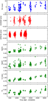 |
Fig. 1 Radial velocity (blue dots), EXORAP (B-band) and APACHE (V -band) photometric(red dots), and spectroscopic (green dots) activity indicator time series for GJ 720 A. |
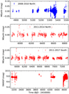 |
Fig. 2 MEarth and SuperWASP photometric time series for GJ 720 A after 2.5σ clipping applied. |
3.2 Photometric time series
Super WASP and MEarth
GJ 720 A was photometrically observed by the Wide Angle Search for Planets (SuperWASP) exoplanet transit survey (Smith & WASP Consortium 2014) and the MEarth (Berta et al. 2012) survey. There were three photometric campaigns using the MEarth telescopes: between 2008 and 2010, from 2011 to 2014, and between 2011 and 2017. The first two campaigns were conducted in the northern hemisphere with a total number of data points of 632 (rms of 8.8 mmag) and 984 (rms of 6.9 mmag), respectively; the third was carried out in the south with 1480 measurements (rms of 6.2 mmag). The original photometric data presented several outliers, and we applied a 2.5σ clipping algorithm to remove them. The outliers were also removed from the SuperWASP photometric data taken between 2004 and 2008. The different photometric time series are presented in Fig. 2.
EXORAP
We also monitored GJ 720 A in the framework of the EXORAP project at the INAF-Catania Astrophysical Observatory with an 80 cm f∕8 Ritchey-Chretien robotic telescope (APT2) located at Serra la Nave on Mt. Etna. We collected ~ 5 yr of B-, V -, R-, and I-band photometry in order to simultaneously obtain photometric and spectroscopic data. We performed data reduction by applying overscan, bias, dark subtraction, and flat fielding with IRAF1 procedures and visual inspection to check the image quality (see Affer et al. 2016 for details). Errors in the individual photometric points include the intrinsic noise (photon noise and sky noise) and the rms of the ensemble stars used for computing the differential photometry. The final dataset contains ~ 240 photometric points for each of the B-, V -, R-, and I-bands distributed over five consecutive seasons, between MJD = 56555 and MJD = 58034 (B filter shown in Fig. 1).
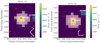 |
Fig. 3 Target pixel files (TPF) of GJ 720 A (TIC122958010) in TESS Sectors 14 and 26. The electron counts are color-coded.The shadowed pixels correspond to the TESS optimal photometric aperture used to obtain the simple aperture photometry (SAP) fluxes. The red dots correspond to the bright nearby stars with TESS magnitude less than 16. The positions of GJ 720 A and GJ 720 B are indicated. |
APACHE
Forty-four of the HADES targets (including GJ 720 A) were also monitored photometrically by the APACHE (A PAthway towards the CHaracterization of Habitable Earths) photometric transit search project (Sozzetti et al. 2013). Our target was very intensively observed by APACHE, having 163 nights over a time span of 1250 days, for a total of 5900 points in the V band. The APACHE photometric observing epochs (binned data are shown in Fig. 1) partially overlap with the spectroscopic observations carried out within HADES; therefore, the photometric and spectroscopic activity data analyzed here are partially simultaneous.
TESS
GJ 720 A (TIC122958010) was observed by TESS in sector 14 between 18 July 2019 and 15 August 2019, and in sector 26 between 18 July 2020 and 15 August 2020. The light curves and the target pixel (TPFs) files for the different sectors were downloaded from the Mikulski Archive for Space Telescopes (MAST), which is a NASA founded project. We verified the pixels in the aperture FITS extension and flagged those used in the optimal photometric aperture in order to check that there is no other source contamination that could affect the transit search. The TPFs files of GJ 720 A with the standard pipeline apertures are shown in Fig. 3. We included in the figure the bright nearby stars with TESS magnitudes less than 16. The visual binary companion GJ 720 B is located outside the standard pipeline apertures, and therefore we can discard some kind of contaminating flux from it. The light curve files provide simple aperture photometry (SAP) fluxes and photometry corrected for systematics effects (PDC; Smith et al. 2012; Stumpe et al. 2014), being the last ones optimized for TESS transit searches.
The information regarding the different photometric surveys, the observing filters and sectors used, the number of days covered per observing season, the number of photometric measurements, and the standard deviation of the differential photometry are summarized in Table 2.
4 Analysis of GJ 720 A
4.1 HARPS-N radial velocities, pre-whitening
The first step of the RV data analysis is the identification of significant periodic signals in the time series. The procedure was applied to the full RV data using the generalized Lomb–Scargle (GLS) periodogram algorithm (Zechmeister & Kürster 2009). We consider significant periods if the power is higher than a chosen false alarm probability (FAP; Zechmeister & Kürster 2009) level of 10% (notable), 1% (prominent), and 0.1% (significant). In Fig. 4, we include the GLS periodograms for the RVs (blue), the spectroscopic activity indicators (green), and the photometry (red) in the frequency range 0.001–0.1 day−1 (1000–10 days in time range). The window function of the HARPS-N RV data is depicted in the top panel of Fig. 4 (yellow line). The second panel of Fig. 4 shows the GLS periodogram for the HARPS-N RV dataset. There are several significant peaks higher than the 0.1% FAP located at 19.5 days (light blue shadowed area), ~ 40 days and ~ 100 days (purple shadowed areas). The most prominent peak is the one at 19.5 days, which we consider our most interesting signal from now on.
In what follows we demonstrate that these three signals are not related to each other by an aliasing effect, which is typically caused by the gaps in the time coverage of the observations (e.g., Dawson & Fabrycky 2010). To identify the presence of possible aliasing phenomena, the spectral window has to be considered. If peaks are seen in the window function, their corresponding aliases will be present in the RV periodograms as falias = ftrue ± mfwindow, where m is an integer, ftrue is the frequency identified in the RV periodogram, and fwindow the frequency from the window function (Deeming 1975). Typical aliases are those associated with the sidereal year, synodic month, sidereal day, and solar day. There are two significant peaks in the window function at the sidereal 1 and 2 yr. Searching for these modulations around the principal peaks of the GLS periodogram of the RV data (19.5, ~ 40, ~ 100 days), we found that secondary (lower) peaks around these three values are due to the aliases at 1 and 2 yr of the spectral windows (Fig. 5). The three main signals in the RV time series are not related to each other by the observation sampling.
In order to verify whether the 19.5 days signal was coherent over the whole observational time baseline, we produced the stacked Bayesian generalized Lomb–Scargle periodogram (s-BGLS, Mortier et al. 2015), which computes the relative probability between peaks. Figure 6 shows the s-BGLS periodogram of the HARPS-N RV data around19.5 days and also around the 40 days activity signal. The s-BGLS showed a continuous increasing of the probability at 19.5 days (left panel of Fig. 6) after around 90 observations, and thereafter the signal became narrower, as expected for a Keplerian signal. On the contrary, the behavior of the signal at ~ 40 days did not show such a high probability and narrow structure. The first maximum of the probability for the ~ 40 days signal was produced after around 90 observations, and thereafter it decreased and increased again for some time. The exact value of the ~40 days signal changed erratically over time, following the increase in the number of observations. This behavior is typical of an incoherent (in amplitude and phase) signal, like that due to the rotational modulation of a star. The coherence of the 19.5 days period established above does not support its identification as the first harmonic of the ~ 40 days period, despite its close value, since it should vary accordingly.
The ~40 days signal that we could attribute to stellar activity, following the pre-whitening method, can be modeled with a sinusoidal curve of 42.1 ± 0.1 days with a semi-amplitude of 3.02 ± 0.44 m s−1 in the RV data. After its removal from the HARPS-N RV data (see panel m of Fig. 4) we found an rms of the residuals of 3.36 m s−1, while the signal at ~100 days (which we attributed to stellar activity) disappears. The signal at 19.5 days remains in the RV GLS periodogram of the residuals and its significance is still far above the FAP level 0.1%. Now we subtract the 19.5 days signal (see panel n of Fig. 4) to observe the behavior of the ~ 40 days signal. The corresponding RV residuals still present the ~40 days signal with the same GLS power, and therefore the same significance. When removing both contributions (19.4 and ~ 40 days peaks, see panel o of Fig. 4) no additional peaks above a 0.1% FAP are present. Those remaining peaks with 1% and 10% are considered a result of the stellar noise.
Photometric seasons available for GJ 720 A.
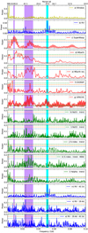 |
Fig. 4 GLS periodograms for GJ 720 A RV data (blue solid lines), photospheric stellar activity (red solid lines), and spectroscopic stellar activity (green solid lines) in the frequency range 0.001–0.1 d−1 (1000–10 days in time range). In all the panels the horizontal dashed lines indicate FAP levels of 10% (blue), 1% (orange), and 0.1% (green). The shadowed areas indicate the region where the RV highest peaks are found. Panels a and b: spectral window (yellow line) and HARPS-N RVs (blue line), respectively. Panel c: SuperWASP binned photometric data. Panels d and e: MEarth binned photometric data and the residuals after removing the highest peak found at ~ 100 days (black vertical dashed line). Panel f: EXORAP B filter. Panel g: APACHE V filter binned photometric data. Panels h–l: HARPS-N NaD1, NaD2, Ca II H & K (S-index), and Hα HARPS-N spectroscopic activity indicators with a linear trend removed. Panel m: HARPS-N RV residuals after removing the 42.1 days signal, indicated as a black vertical dashed line. Panel n: HARPS-N RV residuals after removing the planet candidate signal at 19.5 days. Panel o: HARPS-N RV residuals after removing the 19.5 and 42.1 days signals. All the activity indicators and the RV data show a significant broad peak between 35 and 45 days. This is likely associated with the rotation period of GJ 720 A. |
4.2 Spectroscopic stellar activity
We identified three principal periodic signals in the GLS periodogram of the RV data (19.5, ~ 40, and ~ 100 days; see Sect. 4.1) where it is necessary to know their origins. The M dwarfs are on average more active than solar-like stars (Leto et al. 1997; Osten et al. 2005), and therefore the effects of the stellar activity (chromospheric or photospheric) can be confused with planetary signals or even hide them. In order to disentangle the effects of activity from true RV variations we analyzed two commonly used chromospheric activity indicators based on measurements of the Hα 6562.82 Å and Ca II H & K 3933.7, 3968.5 Å lines (S-index) and also the sodium doublet (NaD1 and NaD2) provided by the TERRA pipeline.
The associated GLS periodograms of all analyzed activity indicators are shown in Fig. 4 (green panels). We also include the FAP levels and the shadowed colored areas that correspond to the principal peaks (19.5, ~ 40, ~ 100 days) identified from the GLS of the RVs. In particular, the NaD1, NaD2, Hα, and S-indexindices present a clear trend in their time series (green panels of Fig. 1). Analyzing the GLS periodogram, we observed this trend as a long-term variability of period >350 d. For this reason we detrended the NaD1, NaD2, S-index, and Hα time series subtracting a straight line before the analysis of the activity indicators. With the activity indices detrended, all of them present some kind of activity centered around 40 days.
In the Hα case the ~ 40 days signal is also present (FAP level <0.1%), but it is not the highest one. For the S-index case, after data detrending, the GLS periodogram shows another long-term variation at 450 days that we also removed (black vertical line in the k panel of Fig. 4). After that we obtained a clear, unique, and significant period at 32.21 ± 0.05 days. The same technique was used to obtain the rotation period of the star published by Suárez Mascareño et al. (2018). The authors derived the stellar rotation at Prot = 34.5 ± 4.7 days with the HARPS-N spectra available to date.
Taking advantage of the available 138 HARPS-N RV data points, we modeled the stellar variability of the S-index (original data that include the trend) using a Gaussian process (GP) regression, which is a more sophisticated method than the pre-whitening one. The fit was performed using juliet (Espinoza et al. 2019), which used radvel (Fulton et al. 2018) to model Keplerian RV signals and george (Ambikasaran et al. 2015) to model the stellar variability with GP. We used an exp-sin-squared kernel multiplied by a squared-exponential kernel, which is included as a default kernel within juliet. This kernel has the form:
 (1)
(1)
where σGP is the amplitude of the GP component given in the same units of the data, Γ is the amplitude of the GP sine-squared component and is dimensionless, α is the inverse squared length scale of the GP exponential component given in d−2, Prot is the period of the GP quasi-periodic component given in d, and τ is the time lag.
All parameters were set with wide priors and in particular the Prot was set free to vary in the range 1–500 days (see Table A.2). The found stellar rotation period, using the GP technique, corresponds to  days with a length-scale median value of 141.28 days (αGP = 5.01 × 10⁻⁵ d−2). Figure 7 shows the GP model that best fits the S-index data, while in Fig. 8 we show the posterior distributions for the GP parameters of the model.
Finally, we note that in all the chromospheric activity indicators studied, no significant signals were identified around 19.5 days (light blue area in Fig. 4), and therefore the hypothesis of a planet candidate at 19.5 days is now more reliable. All the chromospheric activity indicators show significant peaks in the range 35–45 days (purple area). In particular, the S-index GP regression analysis established the stellar rotation period at  days. We conclude that all the possible signals identified in the RV GLS periodogram around this value could be related to stellar activity effects or to the stellar rotation period, and therefore their Keplerian nature can be ruled out. The different activity indicators used here track different features in the stellar atmosphere, and considering the differential rotation of the star it is plausible that they do not yield exactly the same periods found in the RV data. The closest period that we could identify in the RV GLS periodogram is 42.1 days.
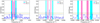 |
Fig. 5 Zoom-in on the GLS periodogram of the HARPS-N RV data of GJ 720 A (blue solid line) around the strongest signals at 19.5 (left panel), 42.1 (center panel), and 112.4 days (right panel). The corresponding values in the frequency domain are 0.05128, 0.02375, and 0.0890 day−1, respectively.The horizontal dashed lines indicate the different FAPs: 0.1% (green), 1% (orange), and 10% (blue). The one- and two-sidereal-year aliases around each of the strongest signals are indicated by cyan and purple vertical solid lines, respectively. |
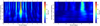 |
Fig. 6 Evolution of the s-BGLS periodogram of the HARPS-N RV data of GJ 720 A. Left panel: the most probable period at 19.5 days (in red) is clearly visible after around Nobs > 80. Right panel:s-BGLS periodogram at around 40 days produced by the stellar variability. |
 |
Fig. 7 GJ 720 A original S-index data together with the best model and the residuals. The fitted GP model (red line) corresponds to an exp-sin-squared kernel multiplied by a squared-exponential kernel modeling the stellar variability. The error bars (green) take into account the jitter (light green). |
4.3 Photometric stellar activity
The M dwarfs have surface inhomogeneities that rotate with the stars. These inhomogeneities cause RV variations due to the distortion of the spectral line profile and can be misinterpreted as signals of Keplerian nature. These inhomogeneities also affect the photometric measurements, which is why a photospheric analysis is crucial in order to avoid unwanted signals as planetary candidates.
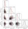 |
Fig. 8 Posterior distributions for the parameters that model the stellar variability using the S-index activity indicator. The vertical dashed lines indicate the 16, 50, and 84% quantiles of the fitted parameters; this corresponds to 1σ uncertainty. The red line shows the median value of each fitted parameter. |
SuperWASP and MEarth
We analyzed the GLS periodograms of the SuperWASP light curve and the MEarth differential light curves (c and d panels of Fig. 4). There are several observing seasons for GJ 720 A within the MEarth survey, thus we studied the differential light curves separately for each observing campaign and for all the seasons together. Due to the huge number of data points obtained with MEarth, we also analyzed the binned differential light curve data. The different analysis for the MEarth available seasons yielded that the variability of the star is better seen in the binned 2008–2010 season, the rest of them are not shown here for clarity. No obvious significant peak can be extracted from the GLS periodograms of the SuperWASP and MEarth light curves. In both cases, there is no clear and narrow peak that can be attributed to the stellar rotation period. The SuperWASP GLS periodogram of the binned data shows the two highest peaks around 40 and 100 days (panel c of Fig. 4). The MEarth GLS periodogram (using the binned data of the season 2008–2010) shows the highest peak around 90 days (panel d of Fig. 4) and, after subtracting its contribution (black vertical line of panel e of Fig. 4), the highest period moves toward ~ 40 days. The periodicities shown in the GLS light curve periodograms agree with those found in the GLS analysis of both RV and spectroscopic activity indicators (light blue and purple areas in Fig. 4). No photospheric or spectroscopic activity signal is detected in the region of interest around 19 days.
EXORAP
We first analyzed the four differential light curves (one for each band) using the GLS periodogram. As the observed photometry shows long-term trends, we pre-whitened the light curves by subtracting from each data series the corresponding third-order polynomial best fit. The periodogram of the pre-whitened B light curve (see panel f of Fig. 4) shows two peaks with FAP <1% at ~34 and ~ 140 days. In the V, R, and I bands we do not detect any signals more significant than 5%, and therefore we do not show them here for clarity. These results suggest a scenario where the photometric variability is due to the effects of an irregularly spotted stellar surface coupled with stellar rotation. This is consistent with the fact that the activity signal is stronger at bluer wavelengths where the contrast between photosphere and cool spots is larger.
APACHE
Giacobbe et al. (2020) has recently published the GJ 720 A rotation period at 33.6 days using the APACHE differential photometric observations. Using the same APACHE binned photometric data we computed the GLS periodogram here (panel g of Fig. 4) corroborating that the highest peak value corresponds to the published value. However, we consider that this value can be regarded as an approximate rotation period of the star because of the presence of other nearby peaks (e.g., ~ 37 days) with a comparable significance. Folding in phase the APACHE light curve at 33.6 days, the amplitude is relatively small (2.5 ± 0.2 mmag) compared with the rms of the data (5.5 mmag) and the mean weighted internal errors (3.9 mmag), which explains why this signal cannot be clearly identified in the GLS periodogram. Analyzing the different photometric epochs separately, we found the ~ 33 and ~ 37 days signals to be the highest ones in the GLS periodogram of the first and fourth APACHE epochs.
TESS
We looked at the TESS light curve using the SAP fluxes to model the stellar activity signatures in order to find a possible stellar rotational period and we used the PDC fluxes for transit searches. The two sectors TESS light curves were analyzed at the same time using a quasi-periodic kernel (QPK) introduced by Foreman-Mackey et al. (2017) of the form
![Mathematical equation: \begin{equation*}k_{i,j}(\tau) = \frac{B}{2+C} e^{-\tau/L} \left[ \cos \left(\frac{2\pi \tau}{P_{\textrm{rot}}} \right) + (1 + C) \right], \end{equation*}](/articles/aa/full_html/2021/05/aa40490-21/aa40490-21-eq4.png) (2)
(2)
where τ = |ti − tj| is the time lag, B and C define the amplitude of the GP, L is the timescale for the amplitude modulation of the GP, and Prot is the period of the quasi-periodic modulations. The juliet light curve models include a dilution factor (Di) which accounts for possible contaminating sources in the aperture that might produce a smaller transit depth than the real value. The model also takes into account the relative out-of-transit target flux (Mi), which is a multiplicative term and not an additive offset. For the transit modeling juliet uses the batman package (Kreidberg 2015). The limb-darkening effect is taken into account with q1 and q2 coefficients, as defined by Kipping (2013), and a quadratic law. Figure 9 shows the SAP (top panels) and PDC data (bottom panels) for the two TESS sectors with the best GP model found. In our case the median value of the posterior distribution for the rotational period for the two TESS different sectors using the SAP fluxes is  and
and  days, respectively. While using the PDC fluxes the median values of the rotational period for the different sectors is
  and
and  days, respectively. The corresponding error bars in both cases (SAP and PDC fluxes) are slightly high, which suggests that there is not a precise determination of the rotation period for GJ 720 A when using the TESS photometric data. TESS time series are shorter than the period we are looking for. Therefore, searching for the rotation period with TESS data does not provide precise results. However, the values obtained agree with those obtained earlier when analyzing the rest of spectroscopic and photometric activity indicators.
A GP model can be also used in order to detrend the TESS light curves before the search of possible transit features. Therefore, using the optimized PDC fluxes and the corresponding previous GP model fit to detrend the light curve, we proceed to search transits. In a first approach searching possible transits we set a wide uniform prior, 1–25 days, for the planetary signal. In a second approach we took advantage of the times of the inferior conjunctions (as derived from the RV curve) in order to estimate the expected times of the transits and to look specifically at those times in the TESS light curves. In both approaches, no transiting planets for GJ 720 A were found.
We concluded after the chromospheric and photospheric analysis that all activity indicators show a significant but broad peak, always in the range of 35–45 days. Therefore, this range can be associated with stellar active regions probably at different latitudes on a differentially rotating star. The GP analysis with the S-index revealed the stellar rotation period to be  days. While the other identified signal by the activity indicators (also seen in RV data) at around 100 days is more likely related to the life cycle of the active regions, as explained by Scandariato et al. (2017) where it was established that the active regions could withstand some stellar rotations. Due to the complex mechanism that the differential rotation can exhibit on M-dwarf stars due to their convective layers, we could not find a narrow signal that determines a precise value for the rotation period in each of the analyzed activity indicators.
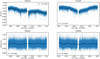 |
Fig. 9 TESS light curves. Top panel: GJ 720 A TESS SAP fluxes (blue points) for the two sectors with the best stellar activity model (black line). Bottom panel: TESS PDC fluxes (blue points) with the best GP model fitted (black line). |
5 Gaussian process regression
The impact that the stellar activity effects can have on the RVs could be different as a function of the stellar magnetic phenomena (e.g., evolving spot configurations). Each target star can have a specific behavior to account for the effects of its stellar variability (e.g., rotating spots, faculae) and the flexibility of the GP algorithms makes their use essential in order to reproduce the stellar phenomena (Perger et al. 2020). However, the diversity of the mathematical GP kernels associated with the true physical phenomena has not been well evaluated to date. Therefore, it is possible that the stellar activity of a specific target could be explicitly better reproduced by one kernel than by another. We decided to test two of the commonly used kernels (exp-sin-squared and QP) to reproduce the stellar variability in order to obtain a robust result of the planet parameters and to know the goodness of the kernels for this specific target.
5.1 Exp-sin-squared kernel, juliet
We used a different approach to analyze the HARPS-N RV data in search of planet candidates using juliet. This technique foresees a simultaneous fit of the stellar activity and the planetary signals. The stellar activity contamination has a significant effect on the derived planetary parameters and to model both signals (stellar and Keplerian) at the same time through the GP regression is essential. The GP kernel implemented here is the exp-sin-squared kernel, previously used and described by Eq. (1). The different implemented models are judged on the basis of the Bayesian Information Criterion (BIC, Liddle 2007). It is based on the log-evidence (ln  ) introducing a penalty term for the parameters used in the model avoiding an overfitting of the data. The BIC value can be described by the following equation:
 (3)
(3)
Here, n is the number of data points, k the number of free parameters to be estimated, and  the maximized value of the likelihood function of the model (see Espinoza et al. 2019, for details). The models are better when the BIC value is lower. The ΔBIC thresholds for considering one model more probable than another with the BIC criterion correspond to i) ΔBIC = 0–2 not worth more than a bare mention, ii) ΔBIC = 2–6 is positive, iii) ΔBIC = 6–10 is strong evidence of preference, and vi) ΔBIC > 10 the model is very strongly preferred.
In a first approach we used a base model (BM), which only includes individual offset and RV jitter, plus a GP kernel (BM + GP model). We used the GP kernel to model the stellar variations observed in the RV data and when analyzing the stellar activity indicators, already discussed in previous sections. We consider uniform distributions for the σGP and Prot parameters of the exp-sin-squared GP kernel with the priors set to  (0, 15) m s−1 and
  (1, 1000) days, respectively.For αGP and ΓGP GP parameters we followed a Jeffrey’s distributions (Jeffreys 1946) setting the prior values as
  (10−20, 104) day−2 and
  (0.01, 100), respectively.We set wide prior values for all four GP parameters in order to test the stellar variability present in the RV data. The expected result with these wide priors, especially the Prot prior that includes both of the highest signals (19.5 and ~40 days) of the RV data, was that the BM + GP model would identify some of them as the Prot value. Surprisingly, the value found for the GP Prot parameter using the HARPS-N RV data corresponds to 38.9 ± 0.05 days, which is close to the Prot value found from the S-index (
 days), and it is placed in the same activity region (30–50 days) determined from the other activity indicators. The final posterior distributions obtained with a base model plus a GP kernel are shown in Fig. 10. The length scale of the GP signal corresponds to a value of ~ 1000 days (αGP = 0.74 × 10⁻⁶ day−2), while the obtained amplitude of the GP model is close to the rms of the RV data. In order to test whether including a linear trend (LT) helps the improvement of the final model, we also fitted the RV data considering the BM plus a GP kernel plus a LT (BM + GP + LT).
In the second approach, we modeled the BM plus one planet (BM + 1pl). In order to explore a blind search of the planet period, without taking into account the recovered information from the GLS periodogram of the RV data, we set a wide uniform prior value for the period of the planet,  (1, 50) days. This prior includes the highest signals of the RV GLS periodogram (19.5 and ~ 40 days). The rest of the priors were set as follows: uniform distributions for the eccentricity
  (0, 0.8), the argument of periastron
  (0, 360) deg, the semi-amplitude
  (0, 10) m s−1, and the time of periastron passage
  (0, 50) days with respect to the time reference 2 456 000. The period found for the planet candidate was
  days, with a time of periastron passage at
  (BJD – 2 456 400).
In a third approach our model was composed of the BM, the GP kernel modeling the activity with a uniform distribution of  (30, 50) days for the Prot GP parameter, plus one planet with a normal distribution for the planet orbital period of
  (19.5, 0.5) days (BM + GP + 1pl). The same model as the previous one but considering the Prot GP parameter as an open uniform distribution,
  (1, 1000) days, was also considered. The planet and GP parameters obtained for these two models were compatible within 1σ error bars. Another test was also considered including a linear trend in the model (BM + GP + 1pl + LT). We note that the narrow prior adopted here for the planet,
  (19.5, 0.5) days, is larger than its final posterior distribution and it is also larger than the final posterior distribution obtained following the second approach where we set a wide uniform prior for the planet (
 (1, 50) days). Therefore, the 19.5 days signal is well characterized and in what follows the assumption of this narrow prior (
 (19.5, 0.5) days) is justified.
In the fourth and last approach we considered the two highest RV signals (19.5 and ~ 40 days) of Keplerian origin. The first model took into account the BM plus two planets (BM + 2pl). The orbital planetary periods were considered with normal distributions  (19.5, 0.5) days and
  (42.1, 0.5) days. The second model took into account the BM plus the same two Keplerian signals (19.5 and ~ 40 days) plus a GP kernel (BM + GP + 2pl) with a wide uniform prior for the Prot in the range 1–1000 days.
The comparison between the different models together with their log-likelihood and BIC values are summarized in Table 3. After that and following the BIC criterion, the best model corresponds to the third approach where together with the base model, an exp-sin-squared GP kernel simulating the stellar contribution and a Keplerian orbit for the planet candidate at 19.5 days were employed. The ΔBIC between the BM + GP model and the BM + GP + 1pl model has a value of 10 for the latter to be strongly preferred. The BIC criterion means that the BM + GP + 1pl model is more likely than the star-only model, and therefore supports the planetary hypothesis at 19.5 days. The detailed distributions and the corresponding priors used to fit the best model are listed in Table A.3. The Prot value derived from the best radial velocity plus Gaussian process (RV + GP) model (35.23 ± 0.11 days) is compatible, within 1 σ, with the Prot obtained from the S-index GP analysis ( days). The amplitude and the length scale of the GP are
  m s−1 and 842 days (αGP = 1.41 × 10⁻⁶ day−2), respectively.
Figure 11 shows the simultaneous fit RV + GP with the best model as a function of the time and the planetary signal of GJ 720 A folded in phase with the orbital period. The final orbital parameters of the planet are listed in Table 4. Figure 12 shows the GLS periodogram of the original RVs (green line) and the corresponding RV GLS periodogram of the residuals after substracting the best model (blue line). This figure shows how the final model produced an optimal removal of all the signals present in the RV data. The rms of the residuals is 1.59 m s−1, around three times smaller than the rms (4.19 m s−1) of the original RV data.
In Fig. 13, we show the posterior distributions of the fitted parameters, this is one planet plus the stellar activity. The planet, GJ 720 Ab, has a minimum mass of 13.64 ± 0.79 M⊕ located at a distance of 0.119 ± 0.002 AU from the host star with an orbital period of 19.466 ± 0.005 days. Due to the low eccentricity value obtained and its error bars we can conclude that the eccentricity is compatible with zero, and therefore our planetary orbit is circular.
A detailed summary of the hyperparameters and priors values used for all the different models followed with juliet are listed in Table A.4. While the final parameter values obtained for each model are summarized in Table A.5.
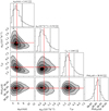 |
Fig. 10 Posterior distributions for the parameters of the GJ 720 A HARPS-N RV data fitting a base model plus an exp-sin-squared GP kernel setting wide prior values for the GP parameters (e.g.,
|

Comparison of different solutions for GJ 720 A using juliet.
5.2 Quasi-periodic kernel, emcee
For completeness, we also performed another GP analysis on the BM+GP and BM+GP+1pl models that differ in the adopted covariance function, the chain sampler, and prior definition, which are uninformative (see Table A.6). This analysis employs the celerite quasi-periodic kernel, described in Eq. (2), and the emcee package (Foreman-Mackey et al. 2013)based on the affine-invariant ensemble sampler for Markov chain Monte Carlo (MCMC) (Goodman & Weare 2010).
The parameter space is covered by 32 walkers, whose initial positions are randomly selected within the prior boundaries. This choice of the initial positions of the walkers requires a burn-in phase to free the chain from very low probability values. Therefore, we set a chain of 50 K steps as burn-in, at the end of which a blob, centered at the maximum probability position, is initialized to feed a second chain. We run the second chain until convergence occurs; in other words, the autocorrelation time of each parameter (see Sokal 1996), evaluated every 10 K steps, varies less than 1% and the chain is 100 times longer than the estimated autocorrelation time. Based on this criterion, the chains converged after 160 K and 440 K steps, respectively, for the BM+GP and BM + GP + 1pl models.
Posterior distributions of the latter model is presented in Fig. 14. BIC parameters for the two models are 766.3 (BM + GP) and 649.5 (BM + GP +1pl). As in the previous analysis, the BIC comparison supports the model in which RV data are described with a Keplerian signal whose planetary parameters are in agreement with those obtained in the previous analysis and reported in Table 4.
Keplerian orbital parameters of GJ 720 Ab from the Gaussian process regression method for the two different approaches that we followed.
5.3 Observing seasons analysis
Looking at the time cadence of the observations we can identify five different observing seasons for our HARPS-N RV data. Only the third and fourth seasons (SIII ~[588, 888] and SIV ~[1238, 1638] days (BJD-2 456 400)) have a significant number of observations, enough to investigate the stability of the planetary signal by applying a GP analysis. Priors of the BM+GP+1pl model using the emcee analysis were adopted, except for the parameter T0 whose prior is (BJD-2 456 400) [0,30]. The estimated planetary parameters for the two subsets are presented in Table 5. The obtained values are generally in agreement with respect to the estimates from the former analysis within 1σ confidence. This does not apply to the semi-amplitude (K1) of the planetary signal, which is systematically larger than the value obtained previously and in the case of SIV is compatible with the previously estimated value within 1.3σ. This effect is related to the inability of the quasi-periodic kernel to model the stellar activity in these two seasons; therefore, because the kernel parameters are not well constrained, a fraction of the stellar signal is absorbed by the semi-amplitude producing larger values of this parameter.
Looking at the two different posterior distributions obtained with each kernel (exp-sin-squared kernel in Fig. 13and QP kernel in Fig. 14), we conclude that exp-sin-squared is the optimal kernel for our target in order to model the stellar variability. The exp-sin-squared kernel is able to identify the same stellar rotational period in the RV data as that obtained from the activity indicators even setting a wide range prior for the GP Prot parameter.
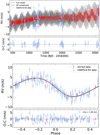 |
Fig. 11 GJ 720 A CARMENES RVs. Top panel: RV time series (blue dots) together with the best model and the residuals. The fitted model (black line) corresponds to the base model plus an exp-sin-squared GP kernel that models the stellar activity at Prot =35.23 ± 0.11 days, and the planetary signal at 19.466 ± 0.005 days. The GP contribution is shown as the red line. The error bars (blue) include the RV jitter (light blue) taken into account. Bottom panel: RVs (blue dots) folded in phase (the base model and the stellar activity were removed) with the orbital period of the planet and its residuals. The best Keplerian solution (black line) has an RV amplitude of 4.72 ± 0.27 m s−1. The red dots correspond to the binned data. The rms of the residuals is 1.59 m s −1. |
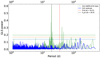 |
Fig. 12 GLS periodograms of the RV data (green line) and the GLS of the residuals(blue line) after subtracting the best model of the RV stellar activity (Prot = 35.23 ± 0.11 days) and the Keplerian signal (19.466 ± 0.005 days) at the same time. The horizontal dashed lines indicate FAP levels of 10% (blue), 1% (orange), and 0.1% (green). The black and red vertical dashed lines indicate the orbital rotational period of the planet and the rotation period of the star, respectively. |
Comparison of the planetary parameters for the two different observed seasons analyzed and the full dataset using emcee.
6 Summary and conclusions
The monitoring of the M dwarf GJ 720 A with the HARPS-N spectrograph during our observing campaign within the HADES program resulted in a sub-Neptune mass detection of a minimum mass of  with a semi-major axis of
  AU in a circular orbit (
 ) that revolves with a period of
  days. All spectroscopic activity indicators (Hα, Ca II H & K, NaD lines) together with the available photometry from the MEarth, SuperWASP, EXORAP, APACHE, and TESS surveys indicate that the other two detected periodicities (~ 40 and ~ 100 days) in the HARPS-N RV data are related to stellar activity phenomena. The stellar rotation period derived here from the S-index activity indicator using a GP regression determined its value at
  days (compatible, within the error bars, with the Prot value (35.23 ± 0.11 days) obtained from the best-fit RV data analysis). The RV signal around 100 days is more likely related to a life cycle of the active regions that persists for some stellar rotations. The different approaches we followed here provided strong arguments in favor of the GJ 720 Ab planet detection. No counterparts in any stellar activity indices were found at the planet orbital period; the stability and the coherence of the planetary signal indicates a long-lived behavior; and the activity and planetary signals are not related with each other by a possible alias phenomena. In addition, we modeled the stellar variability and the possible Keplerian signals in a simultaneous way using a GP regression and employing two independent analyses (juliet and emcee) for completeness. We analyzed different possible models (e.g., GP only, GP + 1pl, GP + 2pl, Keplerian signals only) that could reproduced the RV signals. The one-planet model at 19.5 days plus a GP kernel modeling the stellar activity was the fit statistically preferred of the different implemented models, and was the fit that determined the final planetary orbital parameters.
We looked at the Kervella et al. (2019) catalog of proper motion anomalies in order to find possible evidence of outer massive companions in the Hipparcos-Gaia absolute astrometry. There is no statistically significant proper motion variation reported for GJ 720 A. Based on the analytical formulation of Kervella et al. (2019), the sensitivity curve for the star implies that companions with masses of 0.27 MJ at 1 AU are ruled out, and massive planets with a few Jupiter masses or larger would produce detectable effects out to a few tens of AU. At the exact separation of GJ 720 Ab the detectable mass from proper motion anomaly is found to be around 15 MJ.
In Fig. 15, we represent the position occupied by GJ 720 Ab in the diagram of known Neptune-type and super-Earth planets discovered only with the RV method around M dwarfs. From this diagram we can observe that more massive planets are located around early M dwarfs (blue dots) while the Earth-like planets are found around mid- and late-M spectral type (red and orange dots). We note that this could be a selection effect because smaller planets can be detected more easily around smaller stars. Our target populates the more massive sub-Neptune part of the diagram at intermediate orbital periods. Thanks to the unbiased forecasting model presented by Chen & Kipping (2017), we predicted the planetary radius as 3.84 . Once an estimation of the planet radius is obtained, we can derive the probability that GJ 720 Ab transits in front of the disk of its host star and the depth that the planet would infer. The corresponding values correspond to 2.2
 % of transit probability and
  (ppm) for the transit depth.
Following the models by Kopparapu et al. (2013, 2014) we estimated the conservative habitable zone limits following the runaway greenhouse effect for 5 M⊕ coefficients. The received effective stellar flux compared to the Sun corresponds to Seff = 1.01 S⊙, and the inner edge of the GJ 720 A habitable zone is placed at 0.24 AU. The habitable zone determination, following Kopparapu et al. (2014), implies that GJ 720 Ab lies inside the inner boundary of the habitable zone where the insolation flux has a value of  S⊕. The theoretical equilibrium temperature (Teq) of GJ 720 Ab was derived by using the Stefan–Boltzmann equation, the stellar parameters of Table 1, and two extreme values of the albedo. In the two extreme cases, A = 0.0 and A = 0.65, the Teq for GJ 720 Ab is 401 ± 32 K for a non-reflecting planet and 309 ± 24 K for the high-reflectance planet.
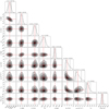 |
Fig. 13 Posterior distributions for the parameters of the best-fit model (BM + GP + 1pl) that describes the planet orbiting GJ 720 A and the stellar variability using juliet. The vertical dashed lines indicate the 16, 50, and 84% quantiles of the fitted parameters; this corresponds to 1σ uncertainty. The red line shows the median value of each parameter. |
 |
Fig. 14 Posterior distribution of the BM + GP + 1pl model in which one sample from the chain over 100 is displayed. For ease of visualization, the offset and jitter parameters are not displayed. The median value of each parameter is plotted with a red line. The results were obtained using the emcee code. The log describing the GP parameters stands for neperian logarithm. |
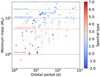 |
Fig. 15 Minimum mass vs. orbital period diagram for known Neptune-type and super-Earth planets (colored dots) around M dwarfs only detected with RV method (available data at http://www.exoplanet.eu). The light blue star indicates the locationof the planet GJ 720 Ab. The color-coding divides the sample by the spectral type of the host star with − 2.0, 0.0, and 7.0 corresponding to K5.0V, M0.0V, and M7.0V, respectively. |
Acknowledgements
This research was supported by the Italian Ministry of Education, University, and Research through the PREMIALEWOW 2013 research project under grant Ricerca di pianeti intorno a stelle di piccola massa. This paper makes use of data from the MEarth Project, which is a collaboration between Harvard University and the Smithsonian Astrophysical Observatory. The MEarth Project acknowledges funding from the David and Lucile Packard Fellowship for Science and Engineering and the National Science Foundation under grants AST-0807690, AST-1109468, AST-1616624 and AST-1004488 (Alan T. Waterman Award), and a grant from the John Templeton Foundation. This work has made use of data from the European Space Agency (ESA) mission Gaia (https://www.cosmos.esa.int/gaia), processed by the Gaia Data Processing and Analysis Consortium (DPAC, https://www.cosmos.esa.int/web/gaia/dpac/consortium). Funding for the DPAC has been provided by national institutions, in particular the institutions participating in the Gaia Multilateral Agreement. E.G.A. acknowledge support from the Spanish Ministry for Science, Innovation, and Universities through projects AYA-2016-79425-C3-1/2/3-P, AYA2015-69350-C3-2-P, ESP2017-87676-C5-2-R, ESP2017-87143-R, and the Spanish State Research Agency (AEI) Project No. MDM-2017-0737 Unidad de Excelencia “María de Maeztu”– Centro de Astrobiología (CAB, CSIC/INTA). A.P. acknowledges support from ASI-INAF agreement 2018-22-HH.0 Partecipazione alla fase B1 della missione ARIEL. We acknowledge support from the Accordo Attuativo ASI-INAF no. 2018.22.HH.O, Partecipazione alla fase B1 della missione Ariel (ref. G. Micela). A.S., M.Pi. acknowledge the financial contribution from the agreement ASI-INAF n.2018-16-HH.0. M.P., I.R. acknowledge support from the Spanish Ministry of Science and Innovation and the European Regional Development Fund through grant PGC2018-098153-B-C33, as well as the support of the Generalitat de Catalunya/CERCA programme. J.I.G.H. acknowledges financial support from Spanish MICINN under the 2013 Ramón y Cajal program RYC-2013-14875. A.S.M. acknowledges financial support from the Spanish Ministry of Science and Innovation (MICINN) under the 2019 Juan de la Cierva Programme.B.T.P. acknowledges Fundación La Caixa for the financial support received in the form of a Ph.D. contract. J.I.G.H., R.R., A.S.M., B.T.P. acknowledge financial support from the Spanish MICINN AYA2017-86389-P.
Appendix A Tables
GJ 720 A data of the HARPS-N observations.
Priors used for the S-index model with juliet.
Priors used for GJ 720 Ab fitting the RV+GP model with juliet.
Summary of all hyperparameters of the different models applied to GJ 720 A RVs implemented with juliet with their corresponding priors and uncertainties.
Summary of the final parameter values of GJ 720 A for the different models that we followed using juliet.
References
- Affer, L., Micela, G., Damasso, M., et al. 2016, A&A, 593, A117 [NASA ADS] [CrossRef] [EDP Sciences] [Google Scholar]
- Affer, L., Damasso, M., Micela, G., et al. 2019, A&A, 622, A193 [NASA ADS] [CrossRef] [EDP Sciences] [Google Scholar]
- Alonso-Floriano, F. J., Morales, J. C., Caballero, J. A., et al. 2015, A&A, 577, A128 [NASA ADS] [CrossRef] [EDP Sciences] [Google Scholar]
- Ambikasaran, S., Foreman-Mackey, D., Greengard, L., Hogg, D. W., & O’Neil, M. 2015, IEEE Trans. Pattern Anal. Mach. Intell., 38, 252 [NASA ADS] [CrossRef] [Google Scholar]
- Anglada-Escudé, G., & Butler, R. P. 2012, ApJS, 200, 15 [NASA ADS] [CrossRef] [Google Scholar]
- Bailer-Jones, C. A. L., Rybizki, J., Fouesneau, M., Mantelet, G., & Andrae, R. 2018, AJ, 156, 58 [NASA ADS] [CrossRef] [Google Scholar]
- Berta, Z. K., Irwin, J., Charbonneau, D., Burke, C. J., & Falco, E. E. 2012, AJ, 144, 145 [NASA ADS] [CrossRef] [Google Scholar]
- Chen, J., & Kipping, D. 2017, ApJ, 834, 17 [Google Scholar]
- Cosentino, R., Lovis, C., Pepe, F., et al. 2012, in Proc. SPIE, Vol. 8446, Ground-based and Airborne Instrumentation for Astronomy IV, 84461V [Google Scholar]
- Cutri, R. M., Skrutskie, M. F., van Dyk, S., et al. 2003, VizieR Online Data Catalog II/246 [Google Scholar]
- Dawson, R. I., & Fabrycky, D. C. 2010, ApJ, 722, 937 [NASA ADS] [CrossRef] [Google Scholar]
- Deeming, T. J. 1975, Ap&SS, 36, 137 [NASA ADS] [CrossRef] [MathSciNet] [Google Scholar]
- Delfosse, X., Forveille, T., Perrier, C., & Mayor, M. 1998, A&A, 331, 581 [NASA ADS] [Google Scholar]
- Dressing, C. D., & Charbonneau, D. 2015, ApJ, 807, 45 [NASA ADS] [CrossRef] [Google Scholar]
- Espinoza, N., Kossakowski, D., & Brahm, R. 2019, MNRAS, 490, 2262 [NASA ADS] [CrossRef] [Google Scholar]
- Foreman-Mackey, D., Hogg, D. W., Lang, D., & Goodman, J. 2013, PASP, 125, 306 [Google Scholar]
- Foreman-Mackey, D., Agol, E., Ambikasaran, S., & Angus, R. 2017, AJ, 154, 220 [Google Scholar]
- Fulton, B. J., Petigura, E. A., Blunt, S., & Sinukoff, E. 2018, PASP, 130, 044504 [NASA ADS] [CrossRef] [Google Scholar]
- Gaia Collaboration (Brown, A. G. A., et al.) 2018, A&A, 616, A1 [NASA ADS] [CrossRef] [EDP Sciences] [Google Scholar]
- Gaia Collaboration (Smart, R. L., et al.) 2021, A&A, 649, A6 [EDP Sciences] [Google Scholar]
- Giacobbe, P., Benedetto, M., Damasso, M., et al. 2020, MNRAS, 491, 5216 [Google Scholar]
- González-Álvarez, E., Micela, G., Maldonado, J., et al. 2019, A&A, 624, A27 [NASA ADS] [CrossRef] [EDP Sciences] [Google Scholar]
- Goodman, J., & Weare, J. 2010, Commun. Appl. Math. Computat. Sci., 5, 65 [Google Scholar]
- Jeffreys, H. 1946, Proc. Roy. Soc. Lond. Ser. A, 186, 453 [Google Scholar]
- Kervella, P., Arenou, F., Mignard, F., & Thévenin, F. 2019, A&A, 623, A72 [NASA ADS] [CrossRef] [EDP Sciences] [Google Scholar]
- Kipping, D. M. 2013, MNRAS, 435, 2152 [Google Scholar]
- Kopparapu, R. K., Ramirez, R., Kasting, J. F., et al. 2013, ApJ, 765, 131 [Google Scholar]
- Kopparapu, R. K., Ramirez, R. M., SchottelKotte, J., et al. 2014, ApJ, 787, L29 [Google Scholar]
- Kreidberg, L. 2015, PASP, 127, 1161 [NASA ADS] [CrossRef] [Google Scholar]
- Leto, G., Pagano, I., Buemi, C. S., & Rodono, M. 1997, A&A, 327, 1114 [NASA ADS] [Google Scholar]
- Liddle, A. R. 2007, MNRAS, 377, L74 [NASA ADS] [Google Scholar]
- Lovis, C., & Pepe, F. 2007, A&A, 468, 1115 [NASA ADS] [CrossRef] [EDP Sciences] [Google Scholar]
- Luyten, W. J. 1979, LHS catalogue, A catalogue of stars with proper motions exceeding 0”5 annually [Google Scholar]
- Maldonado, J., Affer, L., Micela, G., et al. 2015, A&A, 577, A132 [NASA ADS] [CrossRef] [EDP Sciences] [Google Scholar]
- Maldonado, J., Scandariato, G., Stelzer, B., et al. 2017, A&A, 598, A27 [NASA ADS] [CrossRef] [EDP Sciences] [Google Scholar]
- Mortier, A., Faria, J. P., Correia, C. M., Santerne, A., & Santos, N. C. 2015, A&A, 573, A101 [NASA ADS] [CrossRef] [EDP Sciences] [Google Scholar]
- Osten, R. A., Hawley, S. L., Allred, J. C., Johns-Krull, C. M., & Roark, C. 2005, ApJ, 621, 398 [NASA ADS] [CrossRef] [Google Scholar]
- Perger, M., García-Piquer, A., Ribas, I., et al. 2017, A&A, 598, A26 [NASA ADS] [CrossRef] [EDP Sciences] [Google Scholar]
- Perger, M., Anglada-Escudé, G., Ribas, I., et al. 2021, A&A 645, A58 [EDP Sciences] [Google Scholar]
- Pinamonti, M., Damasso, M., Marzari, F., et al. 2018, A&A, 617, A104 [NASA ADS] [CrossRef] [EDP Sciences] [Google Scholar]
- Queloz, D., Henry, G. W., Sivan, J. P., et al. 2001, A&A, 379, 279 [NASA ADS] [CrossRef] [EDP Sciences] [Google Scholar]
- Reiners, A., Joshi, N., & Goldman, B. 2012, AJ, 143, 93 [NASA ADS] [CrossRef] [Google Scholar]
- Reiners, A., Zechmeister, M., Caballero, J. A., et al. 2018, A&A, 612, A49 [NASA ADS] [CrossRef] [EDP Sciences] [Google Scholar]
- Robertson, P., Mahadevan, S., Endl, M., & Roy, A. 2014, Science, 345, 440 [NASA ADS] [CrossRef] [Google Scholar]
- Scandariato, G., Maldonado, J., Affer, L., et al. 2017, A&A, 598, A28 [NASA ADS] [CrossRef] [EDP Sciences] [Google Scholar]
- Schweitzer, A., Passegger, V. M., Cifuentes, C., et al. 2019, A&A, 625, A68 [NASA ADS] [CrossRef] [EDP Sciences] [Google Scholar]
- Smith, A. M. S., & WASP Consortium 2014, Contrib. Astron. Observ. Skalnate Pleso, 43, 500 [Google Scholar]
- Smith, J. C., Stumpe, M. C., Van Cleve, J. E., et al. 2012, PASP, 124, 1000 [Google Scholar]
- Sokal, A. 1996, in Monte Carlo Methods in Statistical Mechanics: Foundations and New Algorithms Note to the Reader [Google Scholar]
- Sozzetti, A., Bernagozzi, A., Bertolini, E., et al. 2013, Eur. Phys. J. Web Conf., 47, 03006 [CrossRef] [Google Scholar]
- Stumpe, M. C., Smith, J. C., Catanzarite, J. H., et al. 2014, PASP, 126, 100 [Google Scholar]
- Suárez Mascareño, A., González Hernández, J. I., Rebolo, R., et al. 2017, A&A, 605, A92 [NASA ADS] [CrossRef] [EDP Sciences] [Google Scholar]
- Suárez Mascareño, A., Rebolo, R., González Hernández, J. I., et al. 2018, A&A, 612, A89 [NASA ADS] [CrossRef] [EDP Sciences] [Google Scholar]
- Tuomi, M., Jones, H. R. A., Barnes, J. R., Anglada-Escudé, G., & Jenkins, J. S. 2014, MNRAS, 441, 1545 [NASA ADS] [CrossRef] [Google Scholar]
- Zechmeister, M., & Kürster, M. 2009, A&A, 496, 577 [NASA ADS] [CrossRef] [EDP Sciences] [Google Scholar]
IRAF is distributed by the National Optical Astronomy Observatories, which are operated by the Association of Universities for Research in Astronomy, Inc., under cooperative agreement with the National Science Foundation.
All Tables
Keplerian orbital parameters of GJ 720 Ab from the Gaussian process regression method for the two different approaches that we followed.
Comparison of the planetary parameters for the two different observed seasons analyzed and the full dataset using emcee.
Summary of all hyperparameters of the different models applied to GJ 720 A RVs implemented with juliet with their corresponding priors and uncertainties.
Summary of the final parameter values of GJ 720 A for the different models that we followed using juliet.
All Figures
|
Fig. 1 Radial velocity (blue dots), EXORAP (B-band) and APACHE (V -band) photometric(red dots), and spectroscopic (green dots) activity indicator time series for GJ 720 A. |
| In the text | |
|
Fig. 2 MEarth and SuperWASP photometric time series for GJ 720 A after 2.5σ clipping applied. |
| In the text | |
|
Fig. 3 Target pixel files (TPF) of GJ 720 A (TIC122958010) in TESS Sectors 14 and 26. The electron counts are color-coded.The shadowed pixels correspond to the TESS optimal photometric aperture used to obtain the simple aperture photometry (SAP) fluxes. The red dots correspond to the bright nearby stars with TESS magnitude less than 16. The positions of GJ 720 A and GJ 720 B are indicated. |
| In the text | |
|
Fig. 4 GLS periodograms for GJ 720 A RV data (blue solid lines), photospheric stellar activity (red solid lines), and spectroscopic stellar activity (green solid lines) in the frequency range 0.001–0.1 d−1 (1000–10 days in time range). In all the panels the horizontal dashed lines indicate FAP levels of 10% (blue), 1% (orange), and 0.1% (green). The shadowed areas indicate the region where the RV highest peaks are found. Panels a and b: spectral window (yellow line) and HARPS-N RVs (blue line), respectively. Panel c: SuperWASP binned photometric data. Panels d and e: MEarth binned photometric data and the residuals after removing the highest peak found at ~ 100 days (black vertical dashed line). Panel f: EXORAP B filter. Panel g: APACHE V filter binned photometric data. Panels h–l: HARPS-N NaD1, NaD2, Ca II H & K (S-index), and Hα HARPS-N spectroscopic activity indicators with a linear trend removed. Panel m: HARPS-N RV residuals after removing the 42.1 days signal, indicated as a black vertical dashed line. Panel n: HARPS-N RV residuals after removing the planet candidate signal at 19.5 days. Panel o: HARPS-N RV residuals after removing the 19.5 and 42.1 days signals. All the activity indicators and the RV data show a significant broad peak between 35 and 45 days. This is likely associated with the rotation period of GJ 720 A. |
| In the text | |
|
Fig. 5 Zoom-in on the GLS periodogram of the HARPS-N RV data of GJ 720 A (blue solid line) around the strongest signals at 19.5 (left panel), 42.1 (center panel), and 112.4 days (right panel). The corresponding values in the frequency domain are 0.05128, 0.02375, and 0.0890 day−1, respectively.The horizontal dashed lines indicate the different FAPs: 0.1% (green), 1% (orange), and 10% (blue). The one- and two-sidereal-year aliases around each of the strongest signals are indicated by cyan and purple vertical solid lines, respectively. |
| In the text | |
|
Fig. 6 Evolution of the s-BGLS periodogram of the HARPS-N RV data of GJ 720 A. Left panel: the most probable period at 19.5 days (in red) is clearly visible after around Nobs > 80. Right panel:s-BGLS periodogram at around 40 days produced by the stellar variability. |
| In the text | |
|
Fig. 7 GJ 720 A original S-index data together with the best model and the residuals. The fitted GP model (red line) corresponds to an exp-sin-squared kernel multiplied by a squared-exponential kernel modeling the stellar variability. The error bars (green) take into account the jitter (light green). |
| In the text | |
|
Fig. 8 Posterior distributions for the parameters that model the stellar variability using the S-index activity indicator. The vertical dashed lines indicate the 16, 50, and 84% quantiles of the fitted parameters; this corresponds to 1σ uncertainty. The red line shows the median value of each fitted parameter. |
| In the text | |
|
Fig. 9 TESS light curves. Top panel: GJ 720 A TESS SAP fluxes (blue points) for the two sectors with the best stellar activity model (black line). Bottom panel: TESS PDC fluxes (blue points) with the best GP model fitted (black line). |
| In the text | |
|
Fig. 10 Posterior distributions for the parameters of the GJ 720 A HARPS-N RV data fitting a base model plus an exp-sin-squared GP kernel setting wide prior values for the GP parameters (e.g.,
|
| In the text | |
|
Fig. 11 GJ 720 A CARMENES RVs. Top panel: RV time series (blue dots) together with the best model and the residuals. The fitted model (black line) corresponds to the base model plus an exp-sin-squared GP kernel that models the stellar activity at Prot =35.23 ± 0.11 days, and the planetary signal at 19.466 ± 0.005 days. The GP contribution is shown as the red line. The error bars (blue) include the RV jitter (light blue) taken into account. Bottom panel: RVs (blue dots) folded in phase (the base model and the stellar activity were removed) with the orbital period of the planet and its residuals. The best Keplerian solution (black line) has an RV amplitude of 4.72 ± 0.27 m s−1. The red dots correspond to the binned data. The rms of the residuals is 1.59 m s −1. |
| In the text | |
|
Fig. 12 GLS periodograms of the RV data (green line) and the GLS of the residuals(blue line) after subtracting the best model of the RV stellar activity (Prot = 35.23 ± 0.11 days) and the Keplerian signal (19.466 ± 0.005 days) at the same time. The horizontal dashed lines indicate FAP levels of 10% (blue), 1% (orange), and 0.1% (green). The black and red vertical dashed lines indicate the orbital rotational period of the planet and the rotation period of the star, respectively. |
| In the text | |
|
Fig. 13 Posterior distributions for the parameters of the best-fit model (BM + GP + 1pl) that describes the planet orbiting GJ 720 A and the stellar variability using juliet. The vertical dashed lines indicate the 16, 50, and 84% quantiles of the fitted parameters; this corresponds to 1σ uncertainty. The red line shows the median value of each parameter. |
| In the text | |
|
Fig. 14 Posterior distribution of the BM + GP + 1pl model in which one sample from the chain over 100 is displayed. For ease of visualization, the offset and jitter parameters are not displayed. The median value of each parameter is plotted with a red line. The results were obtained using the emcee code. The log describing the GP parameters stands for neperian logarithm. |
| In the text | |
|
Fig. 15 Minimum mass vs. orbital period diagram for known Neptune-type and super-Earth planets (colored dots) around M dwarfs only detected with RV method (available data at http://www.exoplanet.eu). The light blue star indicates the locationof the planet GJ 720 Ab. The color-coding divides the sample by the spectral type of the host star with − 2.0, 0.0, and 7.0 corresponding to K5.0V, M0.0V, and M7.0V, respectively. |
| In the text | |
Current usage metrics show cumulative count of Article Views (full-text article views including HTML views, PDF and ePub downloads, according to the available data) and Abstracts Views on Vision4Press platform.
Data correspond to usage on the plateform after 2015. The current usage metrics is available 48-96 hours after online publication and is updated daily on week days.
Initial download of the metrics may take a while.