| Issue |
A&A
Volume 649, May 2021
|
|
|---|---|---|
| Article Number | A32 | |
| Number of page(s) | 28 | |
| Section | Interstellar and circumstellar matter | |
| DOI | https://doi.org/10.1051/0004-6361/202040221 | |
| Published online | 06 May 2021 | |
Submillimeter imaging of the Galactic Center starburst Sgr B2
Warm molecular, atomic, and ionized gas far from massive star-forming cores★,★★,★★★
1
Instituto de Física Fundamental (CSIC). Calle Serrano 121-123,
28006
Madrid,
Spain
e-mail: This email address is being protected from spambots. You need JavaScript enabled to view it.
2
RAL Space, Rutherford Appleton Laboratory,
Oxfordshire,
OX11 0QX, UK
Received:
23
December
2020
Accepted:
26
March
2021
Abstract
Context. Star-forming galaxies emit bright molecular and atomic lines in the submillimeter and far-infrared (FIR) domains. However, it is not always clear which gas heating mechanisms dominate and which feedback processes drive their excitation.
Aims. The Sgr B2 complex is an excellent template to spatially resolve the main OB-type star-forming cores from the extended cloud environment and to study the properties of the warm molecular gas in conditions likely prevailing in distant extragalactic nuclei.
Methods. We present 168 arcmin2 spectral images of Sgr B2 taken with Herschel/SPIRE-FTS in the complete ~450−1545 GHz band. We detect ubiquitous emission from mid-J CO (up to J = 12−11), H2O 21,1−20,2, [C I] 492, 809 GHz, and [N II] 205 μm lines. We also present velocity-resolved maps of the SiO (2−1), N2H+, HCN, and HCO+ (1−0) emission obtained with the IRAM 30 m telescope.
Results. The cloud environment (~1000 pc2 around the main cores) dominates the emitted FIR (~80%), H2O 752 GHz (~60%) mid-J CO (~91%), [C I] (~93%), and [N II] 205 μm (~95%) luminosity. The region shows very extended [N II] 205 μm emission (spatially correlated with the 24 and 70 μm dust emission) that traces an extended component of diffuse ionized gas of low ionization parameter (U ≃ 10−3) and low LFIR / MH2 ≃ 4−11 L⊙M⊙−1 ratios (scaling as ∝Tdust6). The observed FIR luminosities imply a flux of nonionizing photons equivalent to G0 ≈ 103. All these diagnostics suggest that the complex is clumpy and this allows UV photons from young massive stars to escape from their natal molecular cores. The extended [C I] emission arises from a pervasive component of neutral gas with nH ≃ 103 cm−3. The high ionization rates in the region, produced by enhanced cosmic-ray (CR) fluxes, drive the gas heating in this component to Tk ≃ 40−60 K. The mid-J CO emission arises from a similarly extended but more pressurized gas component (Pth / k ≃ 107 K cm−3): spatially unresolved clumps, thin sheets, or filaments of UV-illuminated compressed gas (nH ≃ 106 cm−3). Specific regions of enhanced SiO emission and high CO-to-FIR intensity ratios (ICO / IFIR ≳ 10−3) show mid-J CO emission compatible with C-type shock models. A major difference compared to more quiescent star-forming clouds in the disk of our Galaxy is the extended nature of the SiO and N2H+ emission in Sgr B2. This can be explained by the presence of cloud-scale shocks, induced by cloud-cloud collisions and stellar feedback, and the much higher CR ionization rate (>10−15 s−1) leading to overabundant H3+ and N2H+.
Conclusions. Sgr B2 hosts a more extreme environment than star-forming regions in the disk of the Galaxy. As a usual template for extragalactic comparisons, Sgr B2 shows more similarities to nearby ultra luminous infrared galaxies such as Arp 220, including a “deficit” in the [C I] / FIR and [N II] / FIR intensity ratios, than to pure starburst galaxies such as M 82. However, it is the extended cloud environment, rather than the cores, that serves as a useful template when telescopes do not resolve such extended regions in galaxies.
Key words: ISM: clouds / photon-dominated region / infrared: ISM / Galaxy: center / ISM: molecules / cosmic rays
Reduced images are also available at the CDS via anonymous ftp to cdsarc.u-strasbg.fr (130.79.128.5) or via http://cdsarc.u-strasbg.fr/viz-bin/cat/J/A+A/649/A32
Herschel is an ESA space observatory with science instruments provided by European-led Principal Investigator consortia and with important participation from NASA.
Includes IRAM 30 m observations. IRAM is supported by INSU/CNRS (France), MPG (Germany), and IGN (Spain).
© ESO 2021
1 Introduction
The interstellar medium (ISM) of galactic nuclei can host extreme conditions driven by the presence of numerous OB-type massive stars (i.e., strong UV radiation fields; Clark et al. 2018), cloud-cloud collisions (e.g., Tsuboi et al. 2015), stellar winds and supernova (SNe) explosions (producing expanding bubbles and widespread shocks; Maeda et al. 2002), enhanced X-ray emission (from accretion onto a super-massive black hole, SMBH), and increased cosmic-ray fluxes (e.g., Zhang et al. 2015). Characterizing the physical conditions and heating mechanisms of the ISM in galactic nuclei (especially the dense molecular gas component, the reservoir that may form new stars) is critical to understand how star formation proceeds in such extreme conditions and how galaxies evolve. With ALMA, it is now possible to study the emission from warm molecular gas in galaxies at increasingly larger redshift. ALMA’s sensitivity allows the detection of redshifted submillimeter (submm) and far-infrared (FIR) rotationally excited molecular lines (e.g., from CO, H2O, HCN, and HCO+) and also the fine-structure atomic lines (e.g., [C I], [O I], [C II], [N II], etc.), which are the main gas coolants.
Far-infrared and submm emission lines are very good tracers of the gas physical conditions and chemistry in extreme star-forming environments, such as those prevailing in merger galaxies (Schirm et al. 2014), starburst (SB) galaxies, and (ultra) luminous infrared galaxies ((U)LIRG; Fischer et al. 2010; van der Werf et al. 2010; Meijerink et al. 2013; Mashian et al. 2015). Ideally, these lines can be used to disentangle the different feedback processes and heating mechanisms operating in their ISM. However, when it comes to star-forming regions of the Milky Way and nearby galaxies, these rest frame frequencies cannot be easily observed with ground-based telescopes due to the poor or null atmospheric transmission.
Giant molecular clouds (GMCs) and their star-forming cores are typically spatially unresolved in extragalactic observations (1″ ≈ 15 pc at a distance of 3 Mpc). Hence, it is not easy to link cloud-scale structure, to galactic structure, to global star formation and evolution. This is clearly a multi-scale problem that benefits from having local templates in which the emission from well characterized environments: photodissociation regions (PDRs), shocks, dense cores, diffuse gas halos, etc. can be spatially resolved. In general, molecular-line observations of local massive star-forming cores (where OB stars are born) should not be directly extrapolated to interpret extragalactic observations because the former ones are not sensitive to the large-scale (often colder and less dense) cloud emission that likely dominates extragalactic observations (e.g., Indriolo et al. 2017). Until very recently, the study of the ISM and star-forming regions targeted either small Galactic (≲1 pc) or large extragalactic (≳1 kpc) spatial scales. The main limitation has been the difficulty to obtain wide-field spectroscopic maps of entire GMCs (scales of tens of pc) in the Milky Way, and to spatially resolve individual GMCs in nearby galaxies. In addition, the FIR and submm windows can only be fully covered from airbone or, preferably, space telescopes.
There is an increasing amount of new extragalactic studies that focus on the smaller spatial scales (≳10 pc; e.g., Schinnerer et al. 2013; Schirm et al. 2014; Wu et al. 2018; Lee et al. 2019). In addition, the implementation of fast mapping techniques and use of broadband spectrometers have made possible to simultaneously map multiple molecular lines over square degree areas of sky (e.g., ≳100 pc2 in Orion B, Pety et al. 2017). Also, the development of multi-beam receivers reduces the mapping time considerably (for square degree maps of Orion A in [C II)158 μm and CO see e.g., Pabst et al. 2019; Goicoechea et al. 2020).
Our aim is to bridge the gap between the small and the intermediate spatial scales in the study of the warm molecular gas in massive star-forming regions of galactic nuclei. We expect to provide a useful template that may help to better interpret the submm spectrum of spatially unresolved star-forming galaxies. Our goal is to determine the properties of the extended cloud environment at spatial scales and conditions close to those prevailing in extragalactic nuclei. In particular, we try to answer the question of which feedback mechanisms dominate in the Galactic Center (GC), with emphasis on the heating mechanisms of the extended molecular gas and the observational signature of X-rays, cosmic rays (CRs), shocks, and stellar radiation1. A related question we study is whether the topology of GMCs affects the propagation of stellar EUV and FUV photons.
In this study we present and analyze 168 arcmin2 (~31 pc × 31 pc) spectral-images of multiple submm lines across the extended cloud environment of the most active high-mass star-forming region of the GC, Sagittarius B2 (Sgr B2). These observations were carried out with the SPIRE–FTS spectrometer (Griffin et al. 2010) on board Herschel (Pilbratt et al. 2010). We expand previous SPIRE–FTS observations of the main massive star-forming cores Sgr B2(N, M, and S) that we introduced in Etxaluze et al. (2013). We also present new velocity-resolved maps of the SiO (J = 2−1), HCN, HCO+, and N2H+ (J = 1−0) emission obtained with the IRAM 30 m telescope in the 3 mm band. We complement these line maps with photometric images of the dust emission obtained with Spitzer (Carey et al. 2009) and Herschel (Molinari et al. 2011). We also make use of 3−79 keV X-ray images taken with NuSTAR (Zhang et al. 2015, and Shuo Zhang priv. comm.).
The paper is organized as follows: in Sect. 2 we give specific details of the Sgr B2 complex and of the observational dataset. In Sect. 3 we present the molecular and atomic emission maps. In Sect. 4 we analyze the dust continuum emission, the excitation of the CO and [C I] lines and discuss the results in the context of PDR and shock models. We also analyze the extended N2H+ emission in relation with the high CR ionization rates. In Sect. 5 we discuss particular tracers of different gas heating mechanisms and compare our results with similar observations of prototypical extragalactic sources, and we discuss specific regions in Sgr B2. In Sect. 6 we summarize our work and conclude.
2 Observations of the Sgr B2 complex
2.1 Sgr B2, a starburst in the Galactic Center
Compared to the disk of the Galaxy, GMCs in the GC are between 10 and 100 times denser and more turbulent (e.g., Morris & Serabyn 1996) but star formation is currently restricted to a few regions like Sgr B2 (e.g., Hatchfield et al. 2020). Sagittarius B2 is the most massive molecular cloud with ongoing high-mass star formation (with lines of sight having gas column densities above  ≳1024 cm−2; e.g., Lis & Goldsmith 1990; Etxaluze et al. 2013; Schmiedeke et al. 2016). At a distance of ~8.18 kpc (e.g., Gravity Collaboration 2019), Sgr B2 is located in the so called central molecular zone (CMZ, see Fig. 1). This is an area of high molecular gas fraction within ~200 pc of the very center (Morris & Serabyn 1996). Sagittarius B2 is one of the most luminous star-forming regions in the Galaxy (~107 L⊙; Goldsmith et al. 1992). Together with Sgr B1 and G0.6−0.0, also in the Sgr B complex, Sgr B2 is located at a projected distance of about 100 pc from the dynamical center of the Milky Way (Sgr A*; see Fig. 1). The Sgr B2 complex lays in the semi-major axis of the 100 pc ring of gas and dust that rotates around the GC (Molinari et al. 2011). This ring is likely located in the x2 orbit system (Binney et al. 1991), and Sgr B2 seems to be placed where orbits x1 and x2 intersect.
Sagittarius B2 contains three main high-mass star-forming cores, Sgr B2(N), Sgr B2(M) and Sgr B2(S), with no less than 49 compact H II regions (Gaume et al. 1995; Ginsburg et al. 2018; Ginsburg & Kruijssen 2018). These cores are embedded in a moderate-density (n(H2) ~105–106 cm−3) molecular cloud of about 5−10 pc (Hüttemeister et al. 1993; Etxaluze et al. 2013; Schmiedeke et al. 2016). The entire complex is surrounded by a larger envelope (~45 pc) (Hüttemeister et al. 1995; Goicoechea et al. 2004), hereafter the Sgr B2 “envelope”, that shows diverse physical conditions. Indeed, given its location in the GC, the whole extended region is a good laboratory to study the properties of the ISM in the nucleus of ULIRG and SB galaxies.
In this study we consider that most, if not all, the submm line and continuum emission inside the white rhombus of Fig. 1 arises from Sgr B2 envelope; that is to say, that all sources in the mapped area are physically associated (we justify this further in the text). The Sgr B2 envelope has a complex structure. The kinematic structure presents a cone shape in the {l, b, vLSR} space, increasing from approximately +20 km s−1 at the edges to approximately +65 km s−1 at the center (Henshaw et al. 2016). Sgr B2(R) and (V) are two additional H II regions ionized by at least one massive O6 star in each region (Martin & Downes 1972; Mehringer et al. 1993). Sgr B2 Deep South (DS; Meng et al. 2019) is located about 2.8′ south of Sgr B2(M). This is a peculiar H II region that shows nonthermal emission (Meng et al. 2019; Padovani et al. 2019) and it hosts a γ-ray source (Yusef-Zadeh et al. 2013). In the southwest of the envelope we find the cloud G0.6−0.0. This region contains no less than four ultracompact H II regions, and is surrounded by an arc, observed in the 3.6 cm radio-continuum, that seems to bridge the southern part of Sgr B2 with the northern part of Sgr B1 (Mehringer et al. 1992). Further to the east we find the G0.66–0.13 region, which was first reported in hard X-ray observations with NuSTAR (Zhang et al. 2015). These authors suggest that this region is a molecular clump and a local column density peak. In addition, this region, which seems to have a hollow hemispherical structure, it is likely a site of ongoing cloud-cloud collision (Tsuboi et al. 2015).
Signatures of ongoing star-formation are found all over the region: very high FIR luminosity, molecular maser emission, X-ray sources, extended, compact, ultra-compact, and hypercompact H II regions, young stellar objects (YSOs), and massive hot cores. These attributes make the complex one of the most prolific star-forming regions in our Galaxy (e.g., Martin & Downes 1972; Whiteoak & Gardner 1983; Benson & Johnston 1984; Mehringer et al. 1992, 1993; Yusef-Zadeh et al. 2009; Ginsburg et al. 2018). From a general perspective, it has been proposed that shocks produced by cloud-cloud collisions triggered the star formation in Sgr B2 starburst (Hasegawa et al. 1994; Sato et al. 2000). Indeed, Sgr B2 could be experiencing an extended (3 pc × 12 pc) star-formation event, not just an isolated starburst within the main star-forming cores (see e.g., Ginsburg et al. 2018).
As in many galactic nuclei, it is not clear what dominates the molecular gas heating in the Sgr B2 envelope. Shocks produced by the peculiar location of Sgr B2 in a region where the x1 and x2 orbits are tangential, a position favorable for cloud-cloud collisions (Hasegawa et al. 1994; Tsuboi et al. 2015; Armijos-Abendaño et al. 2020a) must play a role. Other studies suggest that both low-velocity shocks and stellar UV radiation permeating a clumpy medium, contribute to the gas heating at large scales (Goicoechea et al. 2004). Previous X-ray observations suggest that the complex is an X-ray reflection nebula because it shows diffuse X-ray emission in the Fe0 Kα line at 6.4 keV (e.g., Koyama et al. 1996; Murakami et al. 2000). In addition, the Fe0 Kα line correlates with the SiO emission, advocating to a relation between shocks and the source of X-rays (Martín-Pintado et al. 2000). Several studies conclude that the region was irradiated with the X-ray emission originated during brief outburst periods of Sgr A* that ended a few hundred years ago (e.g., Zhang et al. 2015; Terrier et al. 2018). In addition, bombardment of low-energy cosmic ray protons (LECRp), from SNe, accretion onto Sgr A*, or local LECR sources, can be related to the X-ray emission as well (Zhang et al. 2015). However, several studies exclude the low-energy cosmic ray electrons (LECRe) as the dominant origin of the Fe0 Kα and hard X-ray continuum emission in Sgr B2 (e.g., Revnivtsev et al. 2004; Terrier et al. 2010; Zhang et al. 2015). For a more detailed discussion on the possible contribution of LECRe and LECRp to the hard X-ray emission in the CMZ, see for example: Zhang et al. (2015); HESS Collaboration (2016); Padovani et al. (2020).
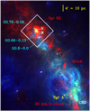 |
Fig. 1 RGB view of about half of the CMZ (~50′ × 60′) in the GC. Red: SPIRE 350 μm tracing cold dust from the most prominent molecular clouds. Green: PACS 70 μm tracing warm dust, mostly in extended PDR-like environments. Blue: MIPS 24 μm tracing hot dust, mostly from ionized regions. The rhombus marks the ~13′ × 13′ area mapped with SPIRE-FTS around Sgr B2(M,N) massive star-forming cores. |
2.2 Herschel/SPIRE-FTS spectroscopic maps of Sgr B2
We obtained 13′ × 13′ submm spectroscopic maps with the SPIRE-FTS instrument (Griffin et al. 2010), and centered them to the coordinates of Sgr B2(M): RA = 17h 47m20.5s, Dec =−28°23′06′′. The spectrometer used two bolometer arrays, the Short Wavelength Spectrometer array (SSW), with 37 detectors covering the wavelength range 194−313 μm (1545−958 GHz) and the Long Wavelength Spectrometer array (SLW), with 19 detectors covering the range 303−671 μm (989−447 GHz). The SLW and SSW detectors sampled an unvignetted field of view of about 2′ in diameter. The major advantage of this multi-beam FTS was that it obtained a complete ~450–1545 GHz spectrum at every detector of the array. This allowed to map nine rotational lines of 12CO simultaneously. These spectra have the maximum spectral resolution allowed by the FTS scanning mechanism (~0.04 cm−1 = 1.2 GHz). Figure 2 shows a selection of these maps and Figs. A.1 and A.2 show all the others.
These maps combine observations from an open time program (OT2_jgoicoec_5; 10.8 h of observing time) and a Must-Do program (DDT_mustdo_1; 4.5 h). In program OT2_jgoicoec_5 (obsID =1342265842), we mapped Sgr B2 at intermediate spatial sampling (one beam spacing) using the bright mode to avoid saturation. The mapping mode was raster scanning with 29 pointings and 4 jiggle positions each. In DDT_mustdo_1 (obsID = 1342252288), we covered the region with sparse sampling (a single pointing of the array per position, 36 in total at roughly two beam spacing). The combined data provide nearly fully spatially sampled maps. We calibrated the data using Herschel Interactive Processing Environment (HIPE; Ott 2010). We adopted the extended emission calibration mode taking into account the diffraction losses and coupling efficiency to a point source model (Swinyard et al. 2014). The resulting integrated line intensities were extracted from the unapodized interferograms after baseline subtraction and classical sinc function fits using the line-fitting tool available in HIPE. The FTS beam (the half power beam width or HPBW) depends on the frequency. It ranges from ~17″ in the SSW detectors to ~42″ in the SLW detectors. However, the FTS HPBW significantly departs from basic diffraction theory (it does not simply scale as the inverse of the frequency; Swinyard et al. 2014). To compare the different line maps (among them and also with photometric images) we convolved all SPIRE-FTS spectral-images to a uniform resolution (HPBW) of 42″ (that of the CO J = 4−3 line) using Gaussian kernels. The typical 1σ line sensitivity in these maps is about 10−9 W m−2 sr−1.
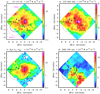 |
Fig. 2 Selection of SPIRE-FTS integrated line intensity maps. The map center coordinates are those of Sgr B2(M) core: RA, Dec = 17h 47m 20.5s, −28° 23′ 06′′. Black stars mark the location of the three massive star-forming cores Sgr B2(N, M, and S). Black triangles mark other H II regions (Mehringer et al. 1992, 1993; Meng et al. 2019). The black dashed circle of radius 2.5′ (~5.0 pc), centered at RA, Dec = 17h 47m 39.7s, −28° 25′ 48′′ marks a specific X-ray irradiated region (Zhang et al. 2015). The pink dashed circles in panel a show Shells 1, 2, and 3 of Tsuboi et al. (2015). White circles show positions A, B, C, and D. |
2.3 Herschel and Spitzer photometric images
We made use of archival photometric images of the FIR and submm dust continuum emission taken with Herschel PACS and SPIRE cameras. These observations are part of the Hi-GAL Herschel Key Project (the Herschel infrared Galactic Plane Survey; Molinari et al. 2010). We retrieved them from the Hi-GAL repository2. We made use of fully calibrated PACS 70 μm and SPIRE 250, 350, and 500 μm images in MJy sr−1 units (we discarded the PACS 160 μm data because they are saturated toward several positions of Sgr B2). These data include a correction of the zero-intensity level using offsets derived from a comparison with Planck/IRAS images (Bernard et al. 2010). The nominal angular resolution (HPBW) of the Hi-GAL Herschel images are ~6″ (70 μm), ~18″ (250 μm), ~25″ (350 μm), and ~36″ (500 μm). In addition, we also made use of the Spitzer/MIPS 24 μm image (~6″ resolution) taken as part of the MIPSGAL Legacy Survey (Carey et al. 2009).
For the dust spectral energy distribution (SED) analysis (see Sect. 4.1) and to compare with the SPIRE-FTS spectral-images, we smoothed these photometric images to a uniform resolution of ~42″ by convolving with Gaussian kernels.
2.4 IRAM 30 m line maps
We complemented the Herschel spectral- and photometric-images with velocity-resolved maps of the 3 mm band (~90 GHz) molecular emission obtained by us with the IRAM 30 m telescope in Pico Veleta (Spain). The size of these maps is 12′ × 12′. We used theE090 receiver, providing an instantaneous bandwidth of 16 GHz per polarization, in combination with the 200 kHz resolution FFT backend. We employed two local oscillator tunings to cover the [84–92]+[100–108] GHz and [92–100]+[108–116] GHz windows. Each map consists of 9 sub-maps observed in the “on-the-fly” mode, scanning the sky in two orthogonal directions. The reference position was taken 20′ away in right ascension. This position was calibrated by observing several positions outside the galactic plane. Here we focused only in the SiO (J = 2−1), N2H+, HCN, and HCO+ (J = 1−0) emission (including the H13CN and H13 CO+ isotopologues). The angular resolution at the target frequencies is ~27″. We carried out these IRAM 30 m observations in August 2014 and 2015 during average summer weather conditions (up to 9 mm of precipitable water vapor). Due to the low declination of the Galactic Center, Sgr B2 was always below 25 degrees of elevation from Pico Veleta. The total observing time was about 28 h and we reached a 1σ sensitivity of ~60 mK per 1 km s−1 resampled velocity channel. We reduced this data with the GILDAS software and subtracted a polynomial baseline of order 1 or 2 avoiding the velocities with molecular emission. We finally gridded the spectra into a data cube through a convolution with a Gaussian kernel of about one third of the HPBW.
3 Results
3.1 The submm spectrum of the Sgr B2 envelope
The mapped area of Sgr B2 envelope extends ~1000 pc2 around the main star-forming cores Sgr B2(N, M, S). To simplify the analysis, we chose four positions at different distances from Sgr B2(M): A (ΔRA, ΔDec) = (4.15′, 1.28′), B (2.95′, 0.52′), and C (0′, −2.67′) as representative positions of the physical conditions in the extended cloud environment, and D (4.5′, 4′), a peculiar and remarkably bright position at the edge of the mapped area. Figure 3 shows the continuum-divided SPIRE-FTS spectra from 450 to 1545 GHz obtained toward the four positions (A, B, C, and D) located at 10.4, 7.2, 6.4, and 15 pc from Sgr B2(M), respectively. Their submm spectra are dominated by rotationally excited CO emission lines, often called “mid-J CO lines”. The brightest ones, those contributing more to the gas cooling, are the J = 6−5, 7−6, and 8−7 lines. The spectra also show the emission from the less abundant 13CO isotopologue (lines from J = 5–4 to 7–6). Other lines also detected in emission include the H2O  = 21,1−20,2 (~752 GHz) line as well as the atomic fine-structure lines [C I] 492, 809 GHz and [N II] 205 μm (Table 1). In addition, the spectra display absorption lines produced by low-energy rotational lines of hydride molecules: CH+, OH+, H2O, HF, H2S, NH, NH2, and NH3 (for a review on hydrides see Gerin et al. 2016). These absorption lines are produced by diffuse clouds in the line of sight toward the GC (in the spiral arms of the Galaxy), by gas in the CMZ, and by gas in the Sgr B2 envelope itself. Herschel/HIFI detected and spectrally resolved these absorption lines toward Sgr B2(N) (e.g., Neill et al. 2014; Indriolo et al. 2015). In these high-resolution HIFI spectra, the ground-state lines of abundant species such as o–H2O (~557 GHz), CH+ (~835 GHz), or p–H2O (~1113 GHz), are saturated to Iν ∕Icont ≃ 0 (i.e., they absorb 100% of continuum) over a broad velocity range: Δv ≃150−200 km s−1. At the low velocity resolution of SPIRE-FTS, inversely proportional to the frequency, these spectrally unresolved lines absorb ~30, ~40, and ~50 % of the continuum emission from Sgr B2(N), respectively. However, their absorption depth across the envelope is smaller (~10, ~20, and ~30 %) which means either that they are not saturated, or that they are saturated over a narrower velocity range. Lines absorbing less than the above percentages (ground-state lines from less abundant species or rotationally excited lines) are certainly not saturated, and thus have absorption depths roughly proportional to e−τ. Even if the continuum level changes from one position to another in the envelope, the absorption depth of these lines do not show remarkable differences from one position to another in these maps. This implies a rather uniform column density of foreground absorbing material.
3.2 Distribution of mid-J CO, [C I] and [N II] 205 μm emission
Figure 2 shows the spatial distribution of the CO J = 10−9 (Fig. 2a), [C I] 809 GHz (Fig. 2b), H2O  = 21,1–20,2 (Fig. 2c), and [N II] 205 μm (Fig. 2d) integrated line emission (i.e., their surface brightness map). The spatial distribution of each CO emission line depends on the rotational number J. Compared to the extended emission of the lower J lines (see Figs. A.1a,b), the higher J lines show amore compact distribution around the main star-forming cores (Figs. A.2g,h). The CO (10−9) surface luminosity around Sgr B2(M, and N) is very high, L10-9 ≃ 150 L⊙ pc−2 (over an area of ~1.3 pc2). For comparison, this is much more luminous than toward a similar area around the Trapezium cluster (that hosts only a few late-type O stars) in Orion A star-forming region (L10−9 ≃ 4 L⊙ pc−2, Goicoechea et al. 2019). In Sgr B2, the CO (10−9) line luminosity remains high through the ~1000 pc2 area of the mapped regions (L10−9 ≃ 0.8 L⊙ pc−2). Interestingly, the CO (6−5) emission does not peak toward the main cores but toward position D. This specific region is discussed in Sect. 5.3.4.
Figure 2b shows the spatial distribution of the [C I] 3P2 −3P1 fine-structure emission at 809 GHz. This line3 from neutral atomic carbon is very widespread through out the envelope (the distribution of the [C I] 3P1−3P0 emission at 492 GHz is similar, see Fig. A.2l). Figure 2c shows that the emission from rotationally excited water vapor (p-H2O 21,1−20,2 line) is also extended over scales of tens of pc. Detailed excitation and radiative transfer models already predicted that this line would be observed in emission over a broad range of physical conditions and background FIR illuminations (Cernicharo et al. 2006).
Finally, Fig. 2d shows a map of the [N II] 3P1−3P0 fine-structure line emission at 205 μm. This line stems from ionized gas. The ionization potential of nitrogen is 14.5 eV, thus the detection of [N II] 205 μm emission implies the presence of ionizing EUV photons, perhaps also X-rays, electron collisional ionization, or proton charge exchanges (e.g., Langer et al. 2015). This line is easily excited by electron collisions because of its low critical density, 173 cm−3 at 8000 K (from collisional rates of Tayal 2011), and because of the small energy difference of the fine-structure levels (ΔE / k = 70 K). Hence, this map traces the spatial distribution of relatively low-density ionized gas. Goicoechea et al. (2004) determined electron densities down to ne ≃ 50−100 cm−3 in the southern envelope (with an average of 240 cm−3) from low-angular resolution (~80″) Infrared Space Observatory observations of the [O III] 52, and 88 μm lines. We suspect that this is the same ionized gas component, which is much more extended than the dense H II regions in the vicinity of young massive stars typically and traced by mm-wave hydrogen radio recombination lines (e.g., Jones et al. 2012). The [N II] 205 μm emission is brighter in the southern envelope and displays a remarkably different spatial distribution than that of the mid-J CO and [C I] lines. Table 2 shows the derived correlation coefficients of the spatial distribution from several gas lines and dust emission wavelengths mapped in Sgr B2.
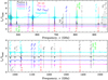 |
Fig. 3 SPIRE-FTS continuum-divided spectra toward four representative positions of Sgr B2 envelope: A in black, B in blue, C in magenta, and D in cyan (the Iν ∕Icont scale appliesto the C spectrum, all the others are shifted). The D spectrum is unapodized, the other three are apodized. |
3.3 Spatial distribution of HCN, HCO+, SiO, and N2H+
3.3.1 Integrated intensity line maps
Figure 4 shows the N2H+ (1−0) (Fig. 4a), HCO+ (1−0) (Fig. 4b), SiO (2−1) (Fig. 4c), and HCN (1−0) (Fig. 4d) integrated line intensity maps (over the entire emission LSR velocity range − 20 to 120 km s−1). Unexpectedly, the spatial distribution of the SiO (2−1) emission, usually associated to warm shocked gas, resembles that of N2H+ (1−0), considered as a tracer of quiescent cold gas (see discussion in Sect. 5.2.1). In Sgr B2 their spatial distribution is extended and moderately correlated4 (ρ = 0.7).
The HCN (1−0) and HCO+ (1−0) emission shows a similar spatial distribution. Their integrated line emission is strongly correlated (ρ = 0.95). The average HCN/H13CN (1−0) and HCO+ / H13CO+ (1−0) line intensity ratios in the mapped area are 7 and 13, respectively. These ratios are lower than the 12C / 13C isotopic abundance ratio derived in Sgr B2 (~20−30; e.g., Langer & Penzias 1990). Therefore, the HCN (1−0) and HCO+ (1−0) emission is optically thick at large spatial scales (for a detailed analysis in the entire CMZ see Jones et al. 2012).
Owing to the strong mm continuum emission from Sgr B2(M, N) cores, these low lying molecular lines turn to absorption (i.e., Tex <Tcont) at many LSR velocities. The absorptions are produced by molecular gas in translucent clouds of the galactic spiral arms located in the line of sight toward the GC (but not related to Sgr B2, e.g., Greaves & Williams 1994) and by gas in the Sgr B2 envelope itself, that absorbs part of the line and continuum emission from the cores. These absorptions are responsible of the apparent lack of molecular emission toward the cores in the integrated line intensity maps of Figs. 4–6.
Spectroscopic and observational parameters of the lines discussed in this work.
3.3.2 Sgr B2 envelope gas velocity components
The gas kinematics in the CMZ is complex and intricate. The average number of velocity components per observed line of sight in the CMZ is 1.6, and >2 in Sgr B2 (Henshaw et al. 2016). In order to ease the discussion, here we split the wide range of emission from Sgr B2 molecular cloud in two different velocity ranges vLSR =[15, 50] km s−1 and [50, 85] km s−1. The vLSR =[50, 85] km s−1 component (see Figs. 5 and 6) covers the main emission velocities of the Sgr B2 molecular cloud (Thiel et al. 2019). Figure 5 shows the spatial distribution of the N2H+ (1−0) and SiO (2−1) emission integrated in the [15, 50] km s−1 and [50, 85] km s−1 velocity ranges separately. Figure 7 shows HCN (1−0), HCO+ (1−0), SiO (2−1), and N2H+ (1−0) line profiles toward the A, B, C, and D positions.
Line emission in the velocity range [15, 50] km s−1 is typically associated to the CMZ and it also includes gas in Sgr B2 envelope (e.g., de Vicente et al. 1997). Figures 5 and 6a,c compare the N2H+ (1−0), SiO (2−1), HCN (1−0), and HCO+ (1−0) emission maps in the [15, 50] km s−1 range. In this velocity range we see two main emission structures. One of them, around position D, is located about 6 arcmin (~15 pc) northeast ofSgr B2(M), and the other, region G0.66–0.13, lays at the southeast of the main cores. This last feature seems to coincide with the hard X-ray continuum emission (Zhang et al. 2015). A remarkable characteristic of the southeastern structure is the very similar spatial distribution of the N2H+ (1−0) and SiO (2−1) emission, and the relative fainter level of the HCN (1−0) and HCO+ (1−0) emission. The northern structure, however, shows bright emission in the N2H+, SiO, HCN and HCO+ lines, as well as in the mid-J CO lines. Interestingly, the SiO (2−1) emission in the LSR velocity range [15, 50] km s−1 and the mid-J CO emission are moderately correlated (ρ ~ 0.8) along the east part of the map (ΔRA ≥ 2′). These specific regions will be discussed in Sect. 5.3.3 and Sect. 5.3.4.
3.4 Spatial distribution of the dust continuum emission
Figure 8 shows the different spatial distribution of the dust continuum emission at 24 μm (Fig. 8a), 70 μm (Fig. 8b), and 350 μm (Fig. 8c). In the southern envelope, the [N II] 205 μm emission spatially correlates with the 24 μm dust emission (Fig. 8a) and also with that at 70 μm (Fig. 8b).
In addition, there are other compact 24 μm emission sources that do not show bright [N II] 205 μm emission counterpart. In particular, those located in the northern part of the envelope. In UV-illuminated environments, the 70 μm continuum emission is often the sum of the dust thermal emission from FUV-heated warm big grains (BGs) and that produced by hotter, stochastically heated, verysmall grains (VSGs; Desert et al. 1990). The latter grains, VSGs, are typically present in the ionized gas and are heated by trapped Ly α radiation (Salgado et al. 2016). In PDR-like environments, the emission from VSGs can contribute to the observed dust continuum emission at λ < 100 μm, especially in the PACS 70 μm images: I70 (Obs.) =I70(BGs) + I70(VSGs). Since the SED of hot VSGs roughly peaks at ~24 μm, this implies that I70 (VSGs) < I24 (VSGs), and thus the observed I24 (VSGs) is an upper limit to I70 (VSGs). Hence, the maximum contribution(in %) of the VSGs emission to the 70 μm continuum emission in PDR environments (R%) is R% = 100⋅ I24 (VSGs) / I70(Obs.) ≥ 100⋅ I70 (VSGs) / I70(Obs.). Figure 8d shows a map of R% at 6″ resolution. The R% ratio increases to ~10% in known H II regions such as Sgr B2(V) and (R), as well as toward G0.6−0.0 (but not toward the main star-forming cores). Even taking into account intensity calibration uncertainties, or a foreground extinction correction of the 24 μm emission (increasing the emission by up to a factor of ~2.5) we conclude that the contribution of VSGs to the 70 μm emission is not large. Indeed, detailed dust emission models of strongly irradiated PDRs, including multiple grain populations, predict that the VSG emission contribution to the FIR continuum emission is ≲5 % (Arab et al. 2012). Hence, the reddish areas of Fig. 8d where R% > 5%, show the greatest contribution from hot VSGs present in ionized gas. Still, the 70 μm emission in Sgr B2 resembles that of 24 μm, and this implies that the H II regions are surrounded by molecular clouds with dusty PDR interfaces.
The continuum emission at longer submm wavelengths stems solely from the BGs population. This emission traces the dust-temperature weighted molecular gas column density, N(H2). The 350 μm emission (Fig. 8c), as well as at longer wavelengths, peaks toward the main star-forming cores and spreads out toward the east, west, and south into the extended envelope.
In the rest of the paper we consider that the observed mid-J CO, [C I] (Figs. 2a,b,c), and submm dust thermal emission (Fig. 8c) arise from Sgr B2 envelope. That is, all emitting sources are physically associated. This seems justified because their spatial distribution has a roughly spherical morphology around the main star-forming cores. In addition, any cloud not related to Sgr B2, but located in the line of sight, will have lower excitation conditions and column densities that are too low to dominate the observed submm line and continuum emission. On the other hand, the extended [N II] 205 μm emission (Fig. 2d) and the mid-infrared emission from hot VSGs (Fig. 8a) do not show such a spherical distribution, and one might argue that they do not belong to the Sgr B2 complex (but see Sect. 5.3.1).
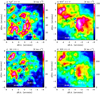 |
Fig. 4 Total integrated line intensity maps (in units K km s−1) of different molecular lines observed with the IRAM 30 m telescope toward the Sgr B2 molecular complex and integrated in the LSR velocity range [ − 20, 120] km s−1. The gray dashed circle marks a specific X-ray irradiated region (Zhang et al. 2015). The pink dashed circles show Shells 1, 2, and 3 of Tsuboi et al. (2015). |
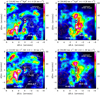 |
Fig. 5 IRAM30 m maps of the N2H+ (1−0) and SiO (2−1) line intensities integrated in the 15−50 km s−1 and 50−85 km s−1 ranges. Contours in panels a and c represent the 2015 hard X-ray emission integrated from 3 to 79 keV (Zhang et al. 2015). Gray: 19 × 10−6 ph s−1 pixel−1. Cyan: 22 × 10−6 ph s−1 pixel−1. Red: (24, 26, 28) ×10−6 ph s−1 pixel−1. Dashed white lines delineate the regions with no X-ray observations. Contours in panels b and d represent the 350 μm emission from 8 to 68 by 20 (103) MJy sr−1. |
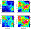 |
Fig. 6 IRAM30 m maps of the HCO+ (1−0) and HCN (1−0) line intensities integrated in the 15−50 km s−1 and 50−85 km s−1 ranges. Contours in panels a and c represent the hard X-Rays emission integrated from 3 to 79 keV, using the 2015 NuSTAR data (Zhang et al. 2015). Gray: 19 × 10−6 ph s−1 pixel−1. Cyan: 22 × 10−6 ph s−1 pixel−1. Red: (24, 26, 28) ×10−6 ph s−1 pixel−1. Dashed white lines delineate the regions with no X-ray observations. Contours inpanels b and d represent the 350 μm data from 8 to 68 by 20 (× 103) MJy sr−1. |
4 Analysis
4.1 Large-scale dust emission: SED fitting
In this section we determine the effective dust temperature (Td), dust opacity (τν), and integrated FIR intensity (IFIR) of BGs froma pixel-to-pixel fit to the dust SED. We fit, based on the Levenberg-Marquardt algorithm, the continuum as a modified black body,
 (1)
(1)
where Bν(Td) is the intensity of a black body at a temperature Td and frequency ν. The dust opacity is parametrized as τν =τν, ref(ν / νref)β, where β is the grain-emissivity index, and we chose as reference frequency, νref, 857 GHz (≃ 350 μm). We let Td and τν, ref be free parameters and use a fixed grain-emissivity index of β = 2, representative of silicate grains (Hirashita et al. 2007, and references therein). Depending on the observed wavelengths, previous studies report emissivity indexes in the range β ~1.1−2.5 in Sgr B2 (Dowell et al. 1999; Etxaluze et al. 2013; Schmiedeke et al. 2016; Arendt et al. 2019). We checked that results obtained by fixing β or leaving it as a free parameter (giving close to 2) do not change Td or τ350 significantly. Figure 9 shows the observed SED and best fit results of the four representative positions in Sgr B2 envelope.
Figure 10a shows the resulting dust temperature map in the region. The average Td is ≃23 K, with a standard deviation5 σ =2 K. The maximum Td value in the envelope is at 21″ (~0.8 pc) south of Sgr B2(M), with Td ≃ 32 K. Far from the main star-forming cores, the warmest dust is located in and around the region G0.6−0.0, where the average dust temperature raises to about 28 K. We note that this analysis implicitly neglects the presence of Td gradients along each line of sight.
From the SED fits we obtain a map of the dust opacity at 350 μm (Fig. 10b). At the angular resolution of the smoothed continuum images (HPBW of 42″), we obtain τ350 μm < 1 in the entiremapped region. In this approach, the dust continuum emission becomes optically thick at wavelengths shorter than ~190 and ~220 μm toward Sgr B2(M) and (N), respectively. In the extended envelope, the continuum emission becomes optically thick only below ~50−100 μm (depending on the position). Therefore, we can safely use the optically thin 350 μm dust emission to derive column densities and cloud masses. We assume that most hydrogen is in molecular form, H2, and derive the molecular gas column density, N(H2), as
 (2)
(2)
through the map, where k350 = 2.38 cm2 g−1 is the dust absorption cross-section per dust mass at 350 μm (Li & Draine 2001) and I350 is the intensity of the 350 μm continuum emission. We adopt the typical interstellar gas-to-dust mass ratio Rgd =100 (Hildebrand 1983), a molecular weight per hydrogen molecule of μ = 2.8 (Kauffmann et al. 2008), and mH the hydrogen atom mass. Figure 10c shows the spatial distribution of the beam-averaged H2 column density along each line of sight. The column densities toward Sgr B2(M) and Sgr B2(N) are 2.8 × 1024 cm−2 and 3.2 × 1024 cm−2, and the dust temperatures are 30.6 and 24.7 K, respectively. Our N(H2) columns are consistent with those derived from a more involved three dimensional dust radiative transfer model: 2.3 × 1024 cm−2 and 2.6 × 1024 cm−2 at a HPBW of 40′′ (see model by Schmiedeke et al. 2016). Therefore, we are confident that our mass estimates are realistic within ~20%.
We derive the molecular gas mass of the cloud as
 (3)
(3)
where Apixel is the area of each pixel in cm2. We obtain  ≃ 107 M⊙ in the mapped region. About ~80% of the mass is in the envelope, whereas ~20% is in the massive star-formingcores, that occupy about 1% of the mapped area. Our derived gas mass agrees with previous estimations (Goldsmith et al. 1990; Schmiedeke et al. 2016). Interestingly, the estimated mass of the X-ray scattering gas in Sgr B2 at a cloud’s radius of about 30 pc is 1.8 × 10⁷ M⊙ (Revnivtsev et al. 2004). Assuming standard interstellar grains, we derived the visual extinction along each line of sight as AV ≃NH / 1.9 ×10²¹ mag (Bohlin et al. 1978). We obtain that AV ranges from ≤ 100 mag in the northwest edges of the map to > 2 × 10³ mag toward the main star-forming cores. These values include at least 25 mag of extinction produced by foreground material not related to Sgr B2 (e.g., Schultheis et al. 1999).
We determined the FIR intensity, IFIR (Fig. 10d), by integrating each fitted SED from 40 to 500 μm (Sanders & Mirabel 1996). We computed the FIR luminosity, LFIR, of a given area as
 (4)
(4)
where D = 8.18 kpc (Gravity Collaboration 2019) and Ω is the solid angle subtended by the area of interest. Figure 10c shows the resulting map of IFIR, where the more luminous regions are those around the massive star-forming cores and G0.6−0.0. The total LFIR in the envelope is ≃ 2.6 ×10⁷ L⊙ (equivalent to a surface luminosity density of 2.7 × 10⁴ L⊙ pc−2), and it is ≃ 0.6 ×10⁷L⊙ (or 5.0 × 10⁵ L⊙ pc−2) in the cores. Thus, ~80% of the total FIR luminosity arises from the large-scale environment around the star-forming cores.
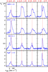 |
Fig. 7 HCN (1−0), HCO+ (1−0), SiO (2−1), and N2H+ (1−0) line profiles toward positions D, A, B, and C. The vertical dashed line at vLSR = 50 km s−1 marks a representative velocity of Sgr B2 envelope. |
4.2 Large scale FUV and EUV radiation illumination
We estimated the approximated flux of stellar FUV photons emitted by OB-type stars (G0 in units of the Habing field) as
![Mathematical equation: \begin{equation*}G_0\simeq\frac{1}{2}\frac{I_{\textrm{FIR}}\,[\textrm{W}\,m^{-2}\,sr^{-1}]}{1.3\times10^{-7}}, \end{equation*}](/articles/aa/full_html/2021/05/aa40221-20/aa40221-20-eq11.png) (5)
(5)
from Hollenbach & Tielens (1999). This relation assumes that the FIR continuum is emitted by FUV-heated dust grains in a face-on PDR. Values of G0 ≃ 2 × 10³ in the envelope would correspond to IFIR contours of ≳ 6 × 10⁻⁴ W m−2 sr−1 in Fig. 10d. Since embedded star-formation (associated with cores of large dust column densities) also produces non-PDR dust continuum emission, this IFIR map should be interpreted as a rough upper limit to G0.
Figure 11 shows a map of the FIR-luminosity to gas-mass ratio (LFIR /  ) computed from the dust SED fits. In the H II regions of high-mass star-forming clouds, this ratio is expected to follow the ionization parameter U = Q(H) ∕4π c neR2, where Q(H) is the number of EUV ionizing photons per second (dominated by Sgr B2(M and N), with about 1050.3 s−1, e.g., Gaume et al. 1995), R is the distance from the ionizing star(s), and ne is the electron density. Our maps observationally support this association because the spatial distribution of the LFIR /
  ratio roughly follows that of [N II] 205 μm and is also very similar to the 24 μm hot dust emission (ρ ≃ 0.8). We find that the spatial distribution of LFIR /
  in Sgr B2 is strongly correlated with
  (ρ ≃ 0.94). Table 3 shows the parameters and ρ coefficients of several FIR- and submm-related magnitudes that show a spatial correlation in the mapped area. The low effective dust temperatures (Td ≃ 20−25 K) explain the generally low LFIR /
  ≲ 5 L⊙M⊙−1 values in Sgr B2 envelope. Toward lines-of-sight of bright [N II] 205 μm and 24 μm dust emission, Td increases above ≃ 25−30 K, leading to LFIR /
  ≃ 4−11 L⊙M⊙−1. The increased Td must be associated with warmer dust in the PDRs that border the extended ionized gas structures. Still, neither Td nor LFIR / Mgas reach the high ratios observed toward much more compact and denser H II regions in the immediate environment of young massive stars (LFIR / Mgas ≃ 100 L⊙M⊙−1 at ~0.2 pc from the Trapezium cluster in Orion, e.g., Goicoechea et al. 2015b). This confirms that, at large spatial scales in Sgr B2, the ionizing radiation has low U values: diluted radiation produced by distant massive stars (for photoionization models of Sgr B2, see Goicoechea et al. 2004). Adopting their average value of ne = 240 cm−3 for the extended ionized gas component and Q(H) ≃ 1050.3 s−1, we obtain U ≃ 10−3 at 6′ (15 pc) from Sgr B2(M). This low ionization parameter is consistent with the low LFIR /
  ratio and Td values that we determine at large scales in Sgr B2 (see model predictions for a broad range of U parameters in Abel et al. 2009). The spatial distribution of the ionizing stars with respect to the extended cloud and the clumpiness of the medium must determine the large-scale effects of this radiation.
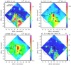 |
Fig. 8 Dust continuum emission at different wavelengths. (a) MIPS 24 μm (VSGs), (b) PACS 70 μm, (c) SPIRE 350 μm, and (d) R% = I24 / I70 × 100 ratio. Black stars mark the location of the massive star-forming cores N, M, and S. Black triangles mark other H II regions (Mehringer et al. 1992, 1993; Meng et al. 2019). The dashed circle marks a specific X-ray irradiated region (Zhang et al. 2015). |
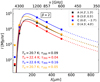 |
Fig. 9 Dust emission: MIPS 24 μm, HiGAL 70, 250, 350, and 500 μm photometric data, all convolved to 42″ resolution (squares, with an intensity uncertainty of ≲15%). Continuous curves show the best-fit BG SEDs of representative positions A, B, C, and D. The 24 μm emissionis produced by hotter VSGs. The area below the continuous curves (40–500 μm) is the integrated FIR intensity (IFIR). |
4.3 Large-scale mid-J CO and [C I]: gas physical conditions
4.3.1 Multi-position population diagrams
In this section we turn back to the properties of the neutral gas and derive the excitation temperature (Tex) and column density (N) of CO and atomic carbon. We first assume that the mid-J CO rotational levels and [C I] fine-structure levels are populated following a Boltzmann distribution at a single excitation temperature, Tex (mid-J CO) and Tex (C), respectively.We analyze their line emission using the population diagram technique to derive Tex and N (see e.g., Goldsmith & Langer 1999).
- (i)
Excitation temperatures as lower limits to Tk:
Figure 12a shows the spatial distribution of the derived excitation temperature for atomic carbon. Tex (C) ranges from 26 K close to the map edges, to ~60 K, around Sgr B2(M). The average Tex(C) value in the mapped area is 36 ± 5 K. If the gas density n(H2) is on the order or lower than the critical density of these fine-structure lines (ncr of a few 103 cm−3, see Table 1), the population of these levels will not exactly be in local thermodynamic equilibrium (LTE) and Tex (C) will be a lower limit to the actual gas kinetic temperature (Tk).
Before determining Tex (mid-J CO), we investigate whether the mid-J CO emission is optically thin. Figure 12b shows a map of the I(CO) /
 J = 5−4 line intensity ratio. This ratio ranges from ~3 toward the main star-forming cores to ≳40 at the map edges. For line intensity ratios significantly below the 12C / 13C isotopic abundance ratio in the GC (~20−30) the CO emission is optically thick or self-absorbed. This is the case of the CO (5−4) emission toward the N, M, S cores and their immediate surroundings (~5−10 pc away). However, in the extended envelope (the spatial scales that dominate the emitted mid-J CO line luminosity) the CO (5−4), and thus all higher J lines, are optically thin. HIFI high-spectral resolution observations of these mid-J 12CO lines toward Sgr B2(M, N) cores show pronounced self-absorption features (Neill et al. 2014; Indriolo et al. 2017). These are produced by the less excited foreground CO in the envelope that absorbs the intense, and optically thick, hot CO emission from the cores. However, we do not expect self-absorption to dominate in the envelope, as we proved that the extended mid-J CO emission is optically thin.
For optically thin line emission, the CO rotational population diagrams provide accurate values for Tex (mid-J CO) and N(mid-J CO). Figure 12c shows the spatial distribution of Tex (mid-J CO) derived from fitting the CO rotational ladder at each position. Figure 12d shows examples of the population diagrams at the four representative positions A, B, C, and D of the extended envelope and Table 4 lists the fit parameters. The extended envelope displays Tex (mid-J CO) in the range 45−65 K. Again, Tex is a lower limit to the kinetic temperature of the CO gas component if n(H2) ≲ncr (these mid-J lines have much higher critical densities, ncr ≃ 105–106 cm−3, than the [CI] lines). The excitation temperature Tex (mid-J CO) toward the main star-forming cores is higher, reaching >100 K. Etxaluze et al. (2013) previously analyzed their complete CO rotational ladder emission.
- (ii)
Column densities of warm CO and atomic carbon:
Figure 13 shows the spatial distribution of the column density of atomic carbon and mid-J CO (hereafter warm CO) inferred from the population diagrams. N(warm CO) ranges from 0.2 × 1017 cm−2 to 2 × 1017 cm−2 in the region around position D. Assuming a range of typical CO abundances with respect to H2, (1−10) ×10−5, these column densities imply that the warm CO is confined to a narrow gas layer of AV ≈ 0.5−5 mag depth (i.e., it does not arise from the entire column of material along each line of sight). The column densities of atomic carbon are higher, from 5 × 1017 cm−2 to 1.7 × 1018 cm−2, and extend from northeast to southwest, through the center. The spatial distribution of the N(C) and N(warm CO) column density maps, as well as the total emission intensity (∑ I[CI] and ∑ ICO; see Table 2) are moderately correlated, with ρ ≳ 0.8.
4.3.2 Gas physical conditions from non-LTE models
To determine the actual gas temperature (Tk) and density (nH2), we first tried to reproducethe observed mid-J CO spectralline energy distributions (SLEDs) and [C I] fine-structure lines with single-slab non-LTE excitation and radiative transfer models. We used the RADEX code (van der Tak et al. 2007), by means of the ndRadex tool (Taniguchi 2019), to generate a large number of models covering a wide range of conditions. As input6 parameters we considered: n(H2) (from 10 to 106 cm−2), Tk (from 102 to 106 K), and the gas column density (N). We comparethe observed CO and [C I] line intensities to those predicted by the models. Table 5 summarizes the best fit model parameters for the four reference positions in the Sgr B2 envelope. The best fit is obtained by finding the minimum root mean square (rms) value7. We find that the best fit models have similar N(C) and N(CO) columns than those derived from the population diagrams. This agrees with optically thin line emission in the extended envelope.
The first remarkable result is that the mid-J CO and [C I] lines seem to trace two different gas components with different physical conditions (lower Tk and density for the [C I]-emitting gas). From the fit results we admit that the best combination of Tk and nH2 is slightly degenerated (in the sense that temperature and density are often anticorrelated). However, the product of these two magnitudes, the gas thermal pressure Pth ∕k = nH Tk (with nH = n(H) + 2n(H2) ≈ 2n(H2) in GC molecular clouds) is more accurately constrained. Figure 14a shows the spatial distribution of the resulting Pth (warm CO). Following the definition of the specific region around the main star-forming cores (N, M, and S) and those of the extended envelope (see Schmiedeke et al. 2016), we derive an average gas thermal pressure Pth(warm CO) = (7.8 ± 1.3) × 106 K cm−3 in the envelope, and Pth (warm CO) = (1.1 ± 0.9) ×108 K cm−3 around the main cores. Since we do not take into account self-absorption of the CO core emission by the envelope, our Pth determination toward Sgr B2(N, M, and S) cores is likely a lower limit. We note that the regions of high thermal pressure extend further east and south into the envelope than the typical definition of the main star-forming cores. These are regions of denser and warmer molecular gas, likely permeated by the strong FUV field that emerges from tens of young OB stars inside the cores and that escapes the region. Although not very different morphologically, the thermal pressure map obtained from the [C I] lines (Fig. 14b) reveals a much lower and more uniform gas pressure component: Pth(C) = (2.8 ± 1.5) × 105 K cm−3 in the envelope.
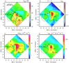 |
Fig. 10 Dust emission properties. (a) Dust temperature derived from SED fist to the photometric data. Contours represent the [N II] 205 μm data. Black: 6 × 10⁻⁸ W m−2 sr−1, gray: 8.5 × 10⁻⁸ W m−2 sr−1, and red: 12 × 10−8 W m−2 sr−1. (b) Map of the dust opacity at 350 μm. (c) Spatial distribution of the molecular gas column density N(H2). (d) Far-IR surface brightness map integrated from 40 to 500 μm. All these maps have a uniform angular resolution of 42′′. |
Summary of FIR- and submm-related magnitudes that are spatially correlated in the mapped area of Sgr B2.
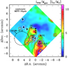 |
Fig. 11 Map of the FIR-luminosity to gas-mass ratio LFIR / Mgas in units of L⊙ / M⊙ per pixel (at an angular resolution of 42″). Contours represent 24 μm emission levels from 3 × 10⁴ MJy sr−1 (red) to 200 MJy sr−1 (blue). |
4.4 PDR and shock models applied to the Sgr B2 envelope
In order to go beyond the previous simple single-slab analysis and to guide our interpretation of such a complex region, in this section we compare the observed molecular and atomic carbon line intensities with the prediction of specific PDR and shock models. These models take into account the gas temperature gradients expected in these environments.
4.4.1 FUV and CR irradiation models
We use the Meudon PDR (Le Petit et al. 2006) to model the Sgr B2 envelope as a constant density cloud illuminated by FUV radiation fields (G0) of different strengths, and adopting enhanced (compared to that in disk GMCs) H2 cosmic-ray ionization rates (ζCR ≲8 × 10⁻¹⁵ s−1 for the LSR velocity range greater than + 40 km s−1 and associated with the dense molecular cloud, see Indriolo et al. 2015). We note that Armijos-Abendaño et al. (2020b) estimate a much lower X-ray ionization rate of ζX ≃ 10−19 s−1 in the envelope. In order to constrain the range of physical conditions that better reproduce the observed mid-J CO lines toward A, B, C, and D positions, we ran several PDR models with different G0 values and gas densitiesnH. Since the observed CO and [C I] emission are very extended, we did not use any filling factor to correct the line intensity predictions.
Figure 15 (left panel) and Table 6 show that the best PDR models fitting the observed mid-J CO line intensities are those with G0 ≃ 103, ζCR = 2 × 10⁻¹⁵ s−1, and nH ≃(1 − 3) × 106 cm−3. While PDR models of lower gas density can still crudely reproduce the observed intensities of the lowest-J CO lines, only high density PDR models reproduce the line intensities beyond Ju > 7 (i.e., beyond the SLED peak, see Fig. 15 left). In these high density models, the mid-J CO emission arises from a narrow layer of warm molecular gas that occupies only ΔAV ≲ 2 mag. This agrees with the low N(warm CO) compared to the much larger total N(H2) columns derived toward each position (equivalent to AV of a few tens of magnitudes). This points to the presence of spatially unresolved clumps or “thin” sheets or filaments of dense molecular gas, exposed to strong FUV fields and distributed uniformly enough throughout the envelope so as to create relatively uniform emission; perhaps similar to the small-scale filamentary structures detected by ALMA at the edges of nearby PDRs (e.g., Goicoechea et al. 2016). Molecular globules and pillars are also readily seen in strongly illuminated clouds at large distances from the exciting stars (Dent et al. 2009; Gahm et al. 2013; Goicoechea et al. 2020). All these overdense gas structures are the consequence of stellar feedback (UV radiation, winds, and shells), mediated by the presence of magnetic fields of different strengths and orientations.
The origin of the [C I] 492, 809 GHz lines in GMCs has been historically difficult to constrain because the observed [C I] emission is generally correlated to that of low-J 13CO lines (e.g., Tauber et al. 1995). Thus, the [C I] emission is often more spatially extended than the predictions of dense PDR models where the emission is confined to a narrow layer in between the C+ and low-J CO emission layers (e.g., Tielens & Hollenbach 1985). In Sgr B2, the [C I] 492, 809 GHz line emission is widespread and relatively uniform at pc scales (Fig. 2b). However, the same dense PDR models that fit the mid-J CO emission greatly underestimate the intensity of the widespread [C I] 492, 809 GHz emission (Fig. 15 right). The only way to reproduce their extended emission is adding a lower density8, nH ≃ (1−2) × 103 cm−3, component illuminated by the same FUV field, G0 ≃ 103, but extending to ΔAV ≃ 20 mag (to match the derived N(C) columns and observed [C I] line intensities). In this component, most of the gas-phase carbon is in atomic form, with N(C)/N(CO) ≃ 10. The gas temperatures predicted by the PDR model are similar to the Tex (C) inferred from the population diagrams (Fig. 12). However, we note that at the nH and Tk of the [C I]-emitting gas, the predicted mid-J CO line emission is negligible.
Figure 16 shows the depth-dependent C+, C, and CO abundance profiles predicted by the low-density (Fig. 16a) and high-density (Fig. 16b) PDR models with G0 = 103. The dotted curves show the predicted [C I] 809 GHz and CO (8−7) line emissivities (in arbitrary units): “extended” along the line of sight for [C I] and “narrow” for the mid-J CO lines. Most of the [C I] emission in Fig. 16a arises from cloud depths where the gas temperature is controlled by ζCR, in the range Tk ≃ 40−60 K for ζCR = (2−6) × 10−15 s−1, and results in xe ≳ 5× 10⁻⁵ and N(C) / N(C+) ≳ 4. In the high-density model of Fig. 16b, the mid-J CO emission arises from denser gas where Tk is set by G0. This produces a steep temperature gradient in the mid-J CO-emitting layers from a few hundred K to about 40 K.
Warm CO and C excitation temperatures and column densities derived from population diagrams toward the reference positions.
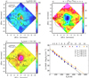 |
Fig. 12 Maps of Tex for (a) atomic carbon and (c) mid-J CO. Contours represent the 13CO J = 5−4 emission from 10−9 W m−2 sr−1 (gray) to 2.8 × 10⁻⁸ W m−2 sr−1 (magenta) tracing high N(H2) regions. (b) Line surface brightness 12CO / 13CO J = 5−4 ratio map. (d) Population diagrams of 12CO lines observed with SPIRE-FTS toward positions A, B, C, and D in Sgr B2 (see Table 4). Dashed curves refer to fits to positions A and D. |
Physical conditions obtained from single-slab non-LTE models.
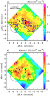 |
Fig. 13 Maps of N(C) and N(warm CO) derived from the population diagram analysis. (a) Contours represent the hard X-Rays integrated from 3 to 79 keV, using the 2015 NuSTAR data (Zhang et al. 2015). Red: (22, 24, 26, 28) ×10−6 ph s−1 pixel−1. Blue: 19 × 10−6 ph s−1 pixel−1. The regions inside the white dashed contours are those of no exposures. |
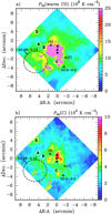 |
Fig. 14 Maps of Pth/k derived fromsingle-slab non-LTE excitation models applied to mid-J CO (upper panel) and [C I] lines (lower panel). |
4.4.2 Shock models of the mid-J CO emission
We also compared the line intensity and shape of mid-J CO SLEDs with predictions of molecular shock models reported by Flower & Pineau Des Forêts (2010). The first conclusion is that high-velocity J-type shock models (vs = 40 km s−1) produce stronger CO emission and shifted to higher-J CO lines. These models neither reproduce the observed mid-J CO line intensities nor the global shape of the CO SLED. For nondissociative C-type shocks, and as vs and nH decreases, the peak of the CO SLED occurs at lower J numbers. Models with nH = 2 × 104 cm−3 and vs = 10−20 km s−1 produce a CO SLED reasonably similar to the observed in Sgr B2 envelope. However, only for position D, a C-type shock model with vs = 20 km s−1 and nH = 2 × 104 cm−3 results in a rms comparable to that of the best PDR model (see Table 6 and left panel of Fig. 15). Although not shown in Fig. 15, J-type and C-type shock models produce little [C I] emission (Neufeld & Dalgarno 1989; Hollenbach & McKee 1989) compared to the intensities observed in Sgr B2.
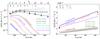 |
Fig. 15 Observed mid-J CO (left panel) and [C I] line intensities (right panel) toward positions A, B, C, and D (shown as triangles). Observed CO and [C I] lines have an intensity uncertainty of ~20%. Continuous curves show predictions from PDR models with different values of G0 and nH (in units of cm−3). Dashed curves in the left panel show C-type shock modelpredictions (from Flower & Pineau Des Forêts 2010). |
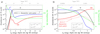 |
Fig. 16 Abundance, line emissivity, and Tk profiles of PDR models with G0 = 103 and ζCR = 2 × 10⁻¹⁵ s−1, consistent with the observed [C I] emission (nH = 103 cm−3; left) and the mid-J CO emission (nH = 106 cm−3; right). We note the different spatial scales (upper axis). |
rms7 of the best PDR and shock models for mid-J CO lines.
4.4.3 Enhanced ionization-rates, extended N2H+ emission
The N2H+ (1−0) emission in Sgr B2 is extended at pc scales. Considering previous observations of nearby star-forming clouds of the Galactic disk, this is an unexpected result. In these clouds, the N2H+ emission traces cold and dense gas shielded from FUV radiation (Caselli et al. 2002). Hence, the N2H+ emission is confined to the dense filamentary “bones” of these clouds and to cold prestellar cores inside them (e.g., Sanhueza et al. 2012; Kirk et al. 2013; Pety et al. 2017; Hacar et al. 2017, 2018).
The main chemical pathway to the formation of N2H+ is the reaction of N2 with H (e.g., Herbst & Klemperer 1973):
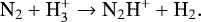 (6)
(6)
The ion H forms after ionization of H2 by cosmic rays, so any enhancement of the ionization rate (including X-rays) will increase the H
 production rate (Indriolo & McCall 2012). The cosmic-ray ionization rate in Sgr B2 is ζCR ≃ (1−10) ×10−15 s−1 (Zhang et al. 2015; Indriolo et al. 2015), a factor of 10−100 higher than the average cosmic-ray ionization rate in clouds of the Galactic disk, where the main N2H+ destruction route is reacting with CO. As the ionization rate increases, so does the abundance of helium ions, ionized by cosmic-ray particles. Hence, destruction of CO by reactions with He+ (in addition to reactions with H
 to form HCO+) becomes increasingly important. In this regime, reactions of He+ with N2 also enhance the formation ofN
 , which further reacts with H2 and increases the N2H+ production. Because of the higher ionization fractions xe at high ζCR, the destruction of both N2H+ and HCO+ becomes dominated by dissociative recombinations with electrons. This leads to a decrease of the HCO+/N2H+ column density ratio as ζCR increases (see also Ceccarelli et al. 2014). This reasoning applies as long as H
 destruction is dominated by reactions with CO (so called chemistry in the “low ionization phase” (LIP); Pineau des Forets et al. 1992; Le Bourlot et al. 1993). In the LIP, and as ζCR increases, protonation reactions with H
 dominate the formation of increasingly more abundant molecular ions such as N2H+.
In the “high ionization phase” (HIP9), however, the abundance of electrons increases to the point where H destruction by electron recombinations becomes comparable to destruction by CO (e.g., Le Bourlot et al. 1993). In this regime, the production of molecular ions from H
 becomes less important and the predicted HCO+ or N2H+ abundances are much lower. Hence, the moderately high G0 and ζCR values in Sgr B2 imply that N2H+ arises fromdense gas (nH >104 cm−3) at relatively large AV (so that xe does not reach the high values of the HIP). Figure 17 show models of this kind for Sgr B2 envelope (G0 = 103, nH = 105 and 106 cm−3, and increasing ζCR). For ζCR = (2−6) × 10−15 s−1, these models predict xe of several 10−8 to several 10−7 at AV = 15 mag. This chemistry is markedly different to that of cold molecular clouds in the disk of the Galaxy, with lower ζCR and thus lower electron and H
 abundances. There, N2H+ is only abundant where CO freezes-out at high extinction depths and cold temperatures (Td ≃Tk < 20 K; see e.g., Caselli et al. 2002; Bergin & Tafalla 2007).
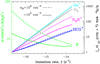 |
Fig. 17 Model predictions for different values of ζCR (and fixed G0 = 103, nH = 105, 106 cm−3, and AV, tot = 15 mag). Continuous curves show the column density enhancement N∕N0 with respect to the models with ζCR,0 = 2 × 10⁻¹⁷ s−1 (roughly theionization rate in disk GMCs). |
5 Discussion
5.1 Tracers of different gas heating mechanisms
In this section we discuss how to observationally distinguish the main heating mechanisms of the warm molecular gas in Sgr B2.
5.1.1 Radiation versus shocks and the CO/FIR intensity ratio
One possible observational diagnostic to discriminate between radiative and mechanical heating is the total CO to FIR luminosity ratio10. Dust grains are more effectively heated in FUV-irradiated environments (producing strong FIR continuum emission). On the other hand, shocks typically heat the molecular gas to higher temperatures, but not the grains. Therefore, we expect higher ICO∕IFIR intensity ratios in shocks than in PDRs (e.g., Meijerink et al. 2013). Figure 18 shows a map of the spatial distribution of the ICO∕IFIR intensity ratio in Sgr B2. The derived ratios range from about 9 × 10⁻⁵ toward 25″ south of Sgr B2(M), to 1.2 ×10⁻³ toward position D. The average ratio in the mapped area is ICO∕IFIR = (4 ± 1)×10−4 (see Table 7). The envelope of Sgr B2 shows a wide range of ICO∕IFIR ratios (see Fig. 18). At first order we see two differentiated regions, one with the low ICO∕IFIR ratios in greenish and blueish, that includes the main star-forming cores and G0.6−0.0 in the south, and coincides with the brightest [N II] 205 μm emitting regions. The second region includes most of the envelope, where the ratio is ≥ 4 ×10⁻⁴, in orangish, and its maximum value peaks toward position D.
The ICO∕IFIR intensity ratio has been observationally measured in prototypical PDRs and shocked gas regions of the Galaxy and in extragalactic sources. It is ≳6×10⁻⁴ toward Orion BN/KL outflows (Goicoechea et al. 2015a), ≃3 × 10⁻⁴ toward the strongly illuminated PDR the Orion Bar (Joblin et al. 2018), and ≃ 10−3 toward Sgr A* and the circumnuclear disk (the CND; where FUV-irradiated shocks likely dominate the hot molecular gas heating; Goicoechea et al. 2013, 2018). In a representative sample of local (U)LIRGs (the HerCULES sample), the LCO∕LFIR ratio is remarkably constant, ~(1.5−3.5) × 10−4, for all LFIR and redshifts. This excludes NGC 6240, which shows a much higher ratio, 1.1×10⁻³ (Rosenberg et al. 2015). NGC 6240 is a luminous merging galaxy in which mechanical widespread shocks, in addition to UV radiation, explains the observed high-J CO lines (Meijerink et al. 2013; Rosenberg et al. 2015). Comparing these intensity ratios with those inferred in Sgr B2 (see Table 7), we conclude that the lower ICO∕IFIR values measured close to the main star-forming cores and toward many locations in the southern part of the envelope resemble more those observed in PDRs. The higher values in the north of the envelope resemble more those seen in shocks.
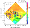 |
Fig. 18 CO to FIR intensity ratio. Contours represent the hard X-ray emission using the 2015 NuSTAR data (S. Zhang priv. comm.; no data inside the areas enclosed by the white dashed lines). Red: (22, 24, 26, 28) ×10−6 ph s−1 pixel−1. Blue: 19 × 10−6 ph s−1 pixel−1. |
Luminosities in Sgr B2 (envelope, main cores, and total).
5.1.2 The [C I] / FIR and [N II] / FIR ratios and their “deficit”
Figure 19a shows the spatial distribution of the I[CI] / IFIR intensity ratio over Sgr B2. The I[CI] / IFIR ratio decreases from ~10−4 in the envelope, to several 10−6 toward the bright FIR star-forming cores (see Table 7). The decrease of I[CI]∕IFIR for increasing FIR intensity reminds of the so called C+/FIR “deficit” seen in observations of the [C II] 158 μm line toward local galaxies hosting vigorous star-formation (e.g., Luhman et al. 1998; Malhotra et al. 2001). This extragalactic deficit may apply to other FIR fine-structure lines ([O I], [O III], [N II], [N III],...) that trace different phases of the ISM (Graciá-Carpio et al. 2011; Herrera-Camus et al. 2018). In Sgr B2 we find that the I[CI] / IFIR intensity ratio is anticorrelated with the FIR emission (ρ = −0.84; see Table 3). The [C I] emission in Sgr B2 only changes by a factor of ~4 whereas IFIR changes by more than two orders of magnitude. Hence the variations of the I[CI] / IFIR are dominated by variations of IFIR, either because G0 reaches high values in the envelope (leading to strong FIR emission of FUV-heated dust) or because the dust column density is very large toward star-forming cores; producing an excess of non-PDR, internally heated, FIR dust emission.
Figure 19b shows the spatial distribution of the I[NII]205/IFIR intensity ratio. The [N II] 205 μm line traces extended low-density ionized gas. The spatial distribution of the I[CI]/IFIR and I[NII]205/IFIR intensity ratios are different. Plotted against the FIR emission, the I[NII]205/IFIR ratio globally decreases for increasing IFIR but the anticorrelation is only apparent in the region around the main star-forming cores (with ρ = − 0.79, Table 3). As we have seen before, the [N II] 205 μm emission is correlated with the 24 μm emission dominated by hot VSGs (see Table 3). Hence, while we do not see the same behavior of the I[NII]205/IFIR and I[CI]492,809∕IFIR intensities ratios, both magnitudes always show the lowest values toward the massive cores of embedded high-mass star formation (very large column densities of dust).
5.2 Sgr B2 as a template for SB and (U)LIRG emission
The spectrum of Sgr B2 main cores has been previously compared to that of prototypical nearby galaxies such as Arp 220, M 82, and NGC 253 (e.g., González-Alfonso et al. 2004; Goicoechea et al. 2004; Martín et al. 2006; Etxaluze et al. 2013; Kamenetzky et al. 2014). Arp 220 is a merger and a SB template of very dusty ULIRGs. The SB galaxy M 82 is considered as an “extragalactic PDR” (Martín et al. 2009). NGC 253 is an isolated spiral galaxy (in an earlier stage of evolution than M 82) in which widespread shocks seem to dominate a significant fraction of the molecular gas heating (Pérez-Beaupuits et al. 2018). NGC 1068 hosts a prototypical CND and an active galactic nuclei (AGN, e.g., Aladro et al. 2015). IC 342 is a face-on spiral galaxy with a nucleus likely similar to our GC (e.g., Röllig et al. 2016). In this section we discuss how the spatially resolved line emission from Sgr B2 cores and envelope compares to the generally unresolved emission from these iconic galaxies.
5.2.1 Widespread and correlated SiO and N2H+ emission
In Sgr B2, the SiO (2−1) and N2H+ (1−0) emission is extended at parsec scales, and is moderately correlated (ρ = 0.7). As the SiO abundance is specifically enhanced by sputtering of silicate grains, bright SiO emission often traces shocked molecular gas (Martin-Pintado et al. 1992; Mikami et al. 1992; Bergin & Tafalla 2007; Jiménez-Serra et al. 2010). In addition, observations of GC clouds show a correlation between the SiO emission and the intensity of the 6.4 keV Fe0 line (Martín-Pintado et al. 2000). The origin of the Fe Kα line may be related to the presence of strong shocks, but also to an enhanced flux of LECRs (Valinia et al. 2000). The first extragalactic detection of SiO and N2H+ were toward the nuclei of the nearby spiral galaxies NGC 253, M 82, Maffei 2, IC 342 and in NGC 6946 only N2H+ (Mauersberger & Henkel 1991). These authors already suggested that SiO and N2H+ could coexist in the warm molecular gas of NGC 253 nucleus.
If we assume a roughly uniform ionization rate in Sgr B2, our maps show that the N2H+ (1−0) / SiO (2−1) intensity ratio decreases in regions where we suspect that the heating of molecular gas is driven or at least affected by shocks. Table 8 lists the N2H+ (1−0) / SiO (2−1) intensity toward different environments of Sgr B2 and in other representative clouds of the GC compared to their observed values in prototypical nearby galaxies. In Sgr B2, the N2H+ (1−0) / SiO (2−1) intensity ratio is relatively uniform (~2−4), and only toward the reference position D the ratio decreases to ~1. This region is also a maximum in the I(CO) / IFIR intensity ratio (≃ 2 × 10⁻³), the emission lines show broad and intricate profiles, and C-type shock models are able to reproduce the observed mid-J CO SLED.
On the other hand, the highest N2H+ (1−0) / SiO (2−1) intensity ratios (~4.5−5) are observed toward G0.6–0.0 and Sgr B2(DS), where the FIR emission is strong (equivalent to an upper limit G0 value of several 104). We suspect that the intermediate ratios between 2 and 3 imply the concerted contribution of both radiative and mechanical heating. The N2H+(1−0) / SiO (2−1) intensity ratios observed toward the prototypical galaxies listed in Table 8 imply that shocks are globally important in ULIRG Arp 220, whereas SB M 82 is dominated by widespread FUV radiation. NGC 253 and NGC 1068 show intermediate values, comparable with regions of the Sgr B2 where UV radiation and widespread shocks drive the heating of the extended molecular gas.
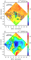 |
Fig. 19 Spatial distribution of the [C I] (492 + 809 GHz) and [NII] 205 μm to FIR intensity ratios in the Sgr B2. (a) Contours represent the hard X-ray emission integrated from 3 to 79 keV, using the 2015 NuSTAR data (same as in Fig. 18). (b) Contours represent the SPIRE 350 μm dust emission. |
Line intensity ratios in Sgr B2 and other sources.
5.2.2 HCO+/ N2H+ and HCO+/ HCN intensity ratios
Our chemical models predict that the HCO+/ N2H+ abundance ratio decreases for increasing CR ionization rates ζCR (Fig. 17). The average value of the HCO+/ N2H+ (1−0) integrated line intensity ratio in Sgr B2 is indeed low ~2, much lower than that observed at (comparable) large spatial scales in disk GMCs (e.g., ~24 in Orion B, Pety et al. 2017). The third column in Table 8 shows that the HCO+/ N2H+ (1−0) intensity ratio observed in the CMZ is in the range 3−5 (Jones et al. 2012). These values are slightly higher than those found in Sgr B2 which either indicates that the ionization rate is higher in Sgr B2 or that the opacity of the HCO+ (1−0) line is higher because of the particularly large column densities of molecular material in Sgr B2. We checked that the H13CO+/ N2H+ (1−0) line ratio multiplied by the GC isotopic ratio 12C / 13C = 30 follows the same behavior and has a typical value of ~5 in the Sgr B2 envelope. Adopting a ratio of ~2 to 5 for a GMC of enhanced ζCR, the HCO+/ N2H+ (1−0) line intensity ratios observed in Arp 220, NGC 253, and IC 342 are closer to those of Sgr B2 (Aladro et al. 2015; Takano et al. 2019), while those of NGC 1068 are slightly higher. The starburst M 82 shows a much higher HCO+/ N2H+ (1−0) intensity ratio, closer to the values observed in disk GMCs such as Orion B, and thus are compatible with molecular clouds of lower CR ionization rates.
Turning to the HCO+/ HCN (1−0) intensity ratio, the average value in Sgr B2 is 0.6, similar to the intensity ratio observed in many locations of the CMZ (Jones et al. 2012) but smaller than the 1.1 average value in Orion B (over large spatial scales; Pety et al. 2017) or at much smaller spatial scales in prototypical PDRs such as the Orion Bar (~1.3; S. Cuadrado, priv. comm.). As in PDRs, pure SB galaxies such as M 82 show HCO+/ HCN (1−0) line intensity ratios above 1. This is a probe of the dominant role of FUV radiation in the gas heating and chemistry of these regions. ULIRGs hosting larger amounts of dense molecular gas, enhanced star-formation rates, and AGNs, often show HCO+/ HCN (1−0) intensity ratios lower than 1 (0.6 in NGC 1068 and 0.4 in Arp 220; Aladro et al. 2015), thus similar to the observed values in Sgr B2. We conclude that in terms of the HCO+/ N2H+ and HCO+/ HCN line intensity ratios, Sgr B2 is closer to the values observed in ULIRG Arp 220.
5.2.3 Submm emission lines in Sgr B2 and in nearby galaxies
The relative abundances of certain molecular species (SiO, N2H+,...) shed light on the presence of UV radiation, CRs, and shocks (if one understands their chemistry). In addition, FIR/submm fine-structure lines and mid-J CO lines directly measure the cooling of the warm neutral gas in star-forming regions. Compared to low-J CO lines, mid-J CO lines have much higherncr and their excitation require higher gas thermal pressures. The detection of extended mid-J CO emission in Sgr B2 reveals the presence of a widespread component of high thermal pressure molecular gas far from the massive star-forming cores. The luminosity emitted by the mid-J CO lines in the extended envelope of Sgr B2 is nearly a factor of ten higher than that emitted from the cores (Table 7). This suggests that the large-scale cloud environment can dominate much of the extragalactic submm line emission.
Kamenetzky et al. (2014) studied the complete CO rotational ladder toward a sample of nearby galaxies, including the prototypical galaxies Arp 220, NGC 253, and M 82. Using their published CO SLEDs we obtain the following excitation temperatures Tex(mid-J CO): 69 ± 2 K, 66 ± 4 K, and 64 ± 4 K, respectively. These values are similar to those of Sgr B2 envelope (Fig. 12c) but lower than toward the massive star-forming cores (Tex ≳ 150 K; Etxaluze et al. 2013). Kamenetzky et al. (2014) fitted their extragalactic CO line fluxes with two gas components (“cold” and “warm”). The gas thermal pressure of their warm component, Pth∕k = nH TK, is ≃ 1.6 × 10⁷ K cm−3 in Arp 220, 1.3 × 10⁷ K cm−3 in NGC 253, and 4.0 × 10⁶ K cm−3 in M 82. The pressures inferred in Arp 220 and NGC 253 are similar to the ones we infer in the extended envelope of Sgr B2 from the mid-J CO lines. In addition, the thermal pressure of their cold gas component (dominated by the lowest-J CO emission) is several 105 K cm−3, very much alike that we derive from the extended [C I]-emitting component in Sgr B2. As a summary, Table 9 compiles the line ratios CO 10−9 / 4−3 (a proxy of high-pressure molecular gas), [N II] 205 μm / [C I] 809 GHz (that seems to measure the contribution of ionizing EUV photons), and [C I] 809 GHz / CO 7−6 in Sgr B2 and in other galactic sources. Again, Sgr B2 shows more similarities with Arp 220 and NGC 253 in these line ratios, and only the [C I] 809 GHz / CO (7−6) is markedly different in NGC 1068 (AGN + SB).
Molecular line intensity ratios in Sgr B2 and in other sources.
5.3 Discussion of specific regions in Sgr B2 complex
We conclude our discussion by zooming again to specific regions of the Sgr B2 complex that show peculiar conditions.
5.3.1 G0.6−0.0: H II regionsin a clumpy medium
The southern and eastern regions of the envelope show bright [N II] 205 μm emission farfrom the massive star-forming cores (Fig. 2d). Radio-continuum observations previously revealed the presence of a diffuse ionized gas component (Mehringer et al. 1992, 1993) and of FIR fine-structure lines at low-angular resolution (Goicoechea et al. 2004). Mehringer et al. (1992) observed the H110α radio recombination line emission and studied the kinematics of the ionized gas in the Sgr B region. The H110α line peaks at vLSR ≃ 55 km s−1 toward G0.6−0.0, which is very similar to one of the emission peaks of the SiO (2−1) and N2H+ (1−0) lines in the same line of sight (vLSR ≃ 51 km s−1). In addition,the emission from H radio recombination lines toward H II regions such as Sgr B2(V, R, AA) peak at analogous velocities than at least two of the molecular lines (sometimes N2H+ and SiO, sometimes HCN and HCO+). Therefore, the ionized and the surrounding molecular gas seem related. The similar velocities in the mapped area suggest that most of the emission sources are physically associated. The origin of the large-scale ionizing radiation is likely the large population of young OB stars in Sgr B2 main cores plus a minor contribution from the less numerous massive stars in the envelope (e.g., at least four late-type O stars in G0.6−0.0; Mehringer et al. 1992). Hence, their natal molecular cores need to be inhomogeneous and clumpy enough so that radiation escapes, diffuses, and illuminates several cloud surfaces along the line of sight (e.g., Tauber & Goldsmith 1990; Goicoechea et al. 2004). This would lead to dilute ionizing radiation at large scales and it is a very plausible scenario to explain the low ionization parameter U and the low LFIR/Mgas ratios inferred in Sgr B2 envelope.
5.3.2 Sgr B2(DS): peculiar H II region, γ-rays, and electrons
The region Sgr B2(DS) is located east of position C (e.g., Ginsburg et al. 2018). Our CO and [C I] maps (Figs. 2 and 4) reveal an emission cavity. However, the [N II] 205 μm map (Fig. 2d) shows an extended secondary emission peak in this region, as well as in the 24 μm dust emission (Fig. 8a). In this particular region, the dust is warmer (Td > 24 K) than the average Td in the envelope, and the 24 μm / 70 μm ratio peaks at R% ≃ 8% (Fig. 8d) suggesting enhanced column densities of ionized gas. In addition, LFIR / Mgas is higher than 5 L⊙/M⊙, which implies that the flux of ionizing photons is higher than the average in the envelope.
The Fermi LAT catalog (Nolan et al. 2012) shows a γ-ray emission source, 2FGL J1747.3-2825c, associated to Sgr B2 (Yusef-Zadeh et al. 2013). This source is located in Sgr B2(DS) (see e.g., Fig. 2a). Recent observations with the VLA reveal an extended H II region that displays a combinationof thermal and nonthermal radio-continuum emission (Meng et al. 2019). The morphology of the thermal emission is clumpy and concentrated, whereas the nonthermal emission is extended and diffuse. Relativistic electrons can be the origin of the nonthermal component (Padovani et al. 2019). Hence, Sgr B2(DS) may be an example of local CR accelerator, having higher CR fluxes than other regions in the envelope, and perhaps altering the C+, C, and CO abundances (see models by e.g., Bisbas et al. 2017). We conclude that perhaps only in this region, accelerated electrons and high-energy radiation produced by relativistic electrons (γ- and X-rays ; e.g., Padovani et al. 2020) contribute to heat the dust, ionize the gas, and clear the molecular gas around Sgr B2(DS).
5.3.3 G0.66–0.13: CRs, X-rays, and shocks
The spatial distribution of the SiO (2−1) and N2H+ (1−0) emission between 15 and 50 km s−1 reveals a very bright extended region in the southeast of Sgr B2 (shown in Figs. 5a,c). The HCN (1−0) and HCO+ (1−0) emission, however, is surprisingly fainter. This region, bright in hard X-ray continuum up to well above 10 keV, was reported as a new cloud feature by Zhang et al. (2015). The 6.4 keV Fe Kα line flux toward this area shows fast variability, that reached a maximum in 2012 and rapidly lessened within one year. These authors concluded that the best possible scenario to explain the Fe Kα flux variability is that G0.66–0.13 is a X-ray reflection nebula affected by past flaring activity from Sgr A* (see also Terrier et al. 2018). Alternatively, Zhang et al. (2015) proposed that if the X-ray emission has actually reached a constant background level, then the emission can be explained as a result of LECRp bombardment.
The spatial distribution of the mid-J CO line emission in G0.66–0.13 follows that of SiO (2−1). Therefore, shocks likely contribute to compress and heat the gas. The N2H+/ SiO and HCO+/ N2H+ intensity ratios are 2.1 and 0.4, respectively (integrated in the +15 to +50 km s−1 velocity range). The low HCO+/ N2H+ ratio suggests that the ionization rate is higher than the average rate in Sgr B2. The spatial correlation of the SiO (2−1) with N2H+ (1−0) emission suggests a common origin, probably related to the presence of shocks and enhanced ionization rates. While the X-ray ionization rate seems too low to affect the gas chemistry (ζX ≃ 10−19 s−1, Armijos-Abendaño et al. 2020b), ζCR is high enough (Zhang et al. 2015) to dominate the ionization in Sgr B2.
The hard X-ray continuum and the 6.4 keV Fe Kα line emission toward G0.66–0.13 seem associated with the SiO (2−1) emission at 15−25 km s−1 velocities (see Figs. 5 and 6, and also Armijos-Abendaño et al. 2020b). Sources able to ultimately drive shocks and generate (hard) X-ray emission would possibly explain a common origin for the enhanced SiO and Fe Kα emission (Martín-Pintado et al. 2000). However, even if shocks with vs ≃ 10−20 km s−1 exist in the envelope, it is unlikely that they generate X-rays or UV radiation (Lehmann et al. 2020). More generally, Tsuboi et al. (2015) suggest the presence of up to 6 shells in the region, one of them as a promising candidate for an ongoing cloud-cloud collision. This particular site, their Shell 3, overlaps with the X-ray-emitting region of G0.66–0.13. Our interpretation is that shocks and enhanced CR fluxes (ultimately leading to enhancedX-ray emission) coexist in G0.66–0.13. The shocked gas in Shell 3 is likely the origin of the bright SiO (2−1) and mid-J CO emission we observe (Figs. 2a and 4). An alternative scenario is that the shocked molecular gas and the enhanced ζCR rates are produced by nearby supernovae remnants (SNRs).
5.3.4 G0.76–0.06: a peculiar shocked region
The region around reference position D (G0.76–0.06) is located about 15 pc away from Sgr B2(M) core. This region shows bright submm- and mm-wave emission lines (see Figs. 2 and 4). Most observational tracers point to shocks driven by the intricate gas dynamics in this region. The SiO (2−1), N2H+, HCN, and HCO+ (1−0) line-profiles toward position D show more than three different velocity components in the LSR velocity range between − 50 km s−1 and 100 km s−1. The derived column density of warm CO toward position D, (2.0 ± 0.4) ×1017 cm−2, is the largestin the map. In addition, the mid-J CO line intensities can be satisfactorily reproduced by C-type shock models (Table 6).
In this region the gas heating is likely driven by shocks and we see that large column densities of warm molecular gas coexists with colder dust (Td ≃ 20−25 K; Fig. 10a). Indeed, the ICO / IFIR luminosity ratio attains its maximum value, ≳ 10−3. Such high ratios are similar to those observed in protostellar outflows (e.g., Goicoechea et al. 2012, 2015a). Furthermore, the detection of very bright SiO (2−1) emission supports the presence of shocks in G0.76–0.06. This region is also a secondary peak in HNCO (Henshaw et al. 2016), a chemical species that is particularly abundant in shocks (e.g., Rodríguez-Fernández et al. 2010).
Given the bright mid-J CO and SiO (2−1) emission and broad line profiles (see also Miyazaki & Tsuboi 2000), one plausible scenario is that gas located in the x1 and x2 orbits collides in this area producing multiple shocks (Binney et al. 1991). An alternative scenario invokes that G0.76–0.06 falls close to the rims of two overlapping expanding shells, likely produced by SN relics (Shells 1 and 2 in Fig. 4), and the rim of Shell 3 (Tsuboi et al. 2015). Higher angular resolution observations will determine whether these shocks trigger star formation.
6 Summary and conclusions
We presented 168 arcmin2 (~1000 pc2) spectral-images of the GC starburst region Sgr B2 taken with Herschel/SPIRE-FTS. We detected widespread and extended emission from 12CO and 13CO rotational ladders (J = 4−3 to J = 12−11 lines), p–H2O 21,1−20,2, [C I] 492, 809 GHz, and [N II] 205 μm lines far from the main star-forming cores. We also presented velocity-resolved maps of the SiO (2−1), N2H+, HCO+, and HCN (1−0) emission taken with the IRAM 30 m telescope. We analyzed this dataset in tandem with Spitzer and Herschel images of the dust emission as well as NuSTAR observations of the hard X-ray continuum. Rather than focusing on the massive star-forming cores, we studied the more extended Sgr B2 envelope (the cloud environment). Although line fluxes at any specific position in the envelope aresmaller than in the cores, the larger area of the envelope means that emission lines integrated over the entire region will be dominated by the envelope and not by the cores. As a result, it is the extended environment, rather than the star-forming cores themselves, that may serve as a useful template when making comparisons to other galaxies where the telescope beams will encompass such extended regions. We summarize our results as follows:
Stellar EUV and FUV photons propagate and permeate the Sgr B2 complex. Owing to the clumpiness of the cloud that surrounds the main star-forming cores Sgr B2(N and M), a fraction of the intense radiation field emitted by young massive stars escapes to the cloud environment. The observed FIR luminosities are equivalent to an upper limit of G0 ≈103 far from these cores. The presence of less prominent local H II regions (more young massive stars) throughout the envelope, especially inthe southern region and G0.6–0.0, adds more UV radiation to the region. The detection of very extended [N II] 205 μm emission, tracing a widespread component of diffuse ionized gas of low ionization parameter U (i.e., dilutedEUV radiation emitted far from the ionized gas) agrees with this scenario. The inferred low ionization parameters, U ≃ 10−3, are consistent with the observed low LFIR / Mgas ≃ 4−11 L⊙M⊙−1 luminosity-to-mass ratios, a proxy of U, and with the cold dust temperatures in the region, with an average of Td ≃ 23 K. The extended [N II] 205 μm emission correlates with the 24 μm emission from hot VSGs (predominantly arising from dust in the ionized gas) and also with the 70 μm emission, arising from bigger grains in the surrounding neutral PDRs.
Spectral-images of the mid-J CO lines (up to J = 12−11) reveal the presence of a widespread component of molecular gas at high thermal-pressure (Pth/k ≃ 107 K cm−3). The observed mid-J CO SLEDs can be explained by PDR models if the emission arises from clumps or thin (ΔAV ~2 mag) sheets of dense molecular gas (nH ≃ 106 cm−3). PDR models with lower gas densities fail to reproduce the observed CO line intensities beyond Ju ≥ 7. The origin of this thin component of FUV-illuminated dense gas can be compressed gas layers at the interfaces of colliding clouds and expanding shells (e.g., Fukui et al. 2021), or be the result of over-pressurized photo-evaporating PDR cloud edges (triggering gas compression, e.g., Hosokawa & Inutsuka 2006; Goicoechea et al. 2016; Bron et al. 2018). The compression of molecular gas can also be produced by shocks triggered by expanding bubbles associated with SNRs or winds from massive stars in the region (e.g., Dwarkadas 2011; Pabst et al. 2020). The presence of bubbles (i.e., of stellar feedback) and cloud-cloud collisions has been invoked in the past (e.g., Martín-Pintado et al. 1999; Tsuboi et al. 2015). The correlation between the CO (7−6) and SiO (2−1) emission suggests that shocks play a role in compressing the gas at many positions.
The [C I] 492, 809 GHz emission reveals a different component of very extended but lower density gas (nH ≃ 103 cm−3). These lines stem from large column densities of neutral gas at lower pressures (Pth/k ≃ 105 K cm−3) than those of the mid-J CO emitting gas. The [C I] intensities can be explained by chemical models with an enhanced ζCR of (2−6) ×10−15 s−1, a factor of ≃10−100 times higher than in disk GMCs. Cosmic rays dominate the heating of this gas component at Tk ≃ 40−60 K and produce significantly larger column densities of C than of C+ and CO.
The enhanced cosmic-ray ionization rate in the dense molecular gas of Sgr B2 leads to enhanced column densities of N2H+ (through more abundant H
 , He+, and N
 ). This leads to extended and widespread N2H+ emission (i.e., not only confined to cold and dense cores and filaments as in disk GMCs). Observationally, the higher ionization fraction of GC clouds is likely responsible of the much lower HCO+/ N2H+ (1−0) line intensity ratios in Sgr B2 (~2) compared to GMCs of the Galactic disk (~25 in Orion B; Pety et al. 2017) or pure starburst galaxies (~20 in M 82; Aladro et al. 2015). In addition, we find that the spatial distribution of the HCO+ and HCN (1−0) emission in Sgr B2 is strongly correlated and shows HCO+/ HCN (1−0) < 1 intensity ratios. This ratio differs from those measured in prototypical PDRs such as the Orion Bar, in Orion B at large spatial scales (Pety et al. 2017), or in M 82, all showing HCO+/ HCN (1−0) > 1. Therefore, in addition to the role of widespread stellar FUV radiation, Sgr B2 is affected by other mechanisms, notably higher cosmic-ray ionization rates and shocks, that contribute to the gas heating and produce its characteristic chemistry. The spatial correlation of the N2H+ (1−0) and SiO (2−1) emission implies that both high ionization rates and shocks coexist at many positions.
Our spectral-images unveil the complexity and more extreme conditions of the ISM of galactic nuclei compared to disk GMCs. Most, but not all, high-mass star formation takes place in three massive cores that radiate ~20% of the FIR luminosity of the mapped region. However, the extended cloud environment dominates the H2O 752 GHz (~60%), mid-J CO (~91%), [C I] (~93%), and [N II] 205 μm (~95%) luminosities.
The N2H+/ SiO, HCO+/ N2H+, and HCO+/ HCN line intensity ratios, the CO SLEDs, and the submm spectra of Sgr B2 envelope resemble more those observed toward the ULIRG galaxy Arp 220, a massive burst of embedded star formation triggered by the collision of two smaller galaxies, and possibly hosting thousands of embedded Sgr B2-like starbursts (Goicoechea et al. 2004; González-Alfonso et al. 2004; Rangwala et al. 2011). However, pure starburst galaxies such as M 82 show markedly different observational characteristics. A major difference is the much higher LFIR /
 > 80 L⊙
 values in Arp 220 and in other galaxies hosting vigorous star formation (Graciá-Carpio et al. 2011). In Sgr B2, LFIR /
  and
and  are strongly correlated (see Table 3), but grains heated by dilute stellar UV photons are relatively cold at large scales. However, ULIRGs produce larger quantities of warmer dust because of the less diluted stellar radiation (more stars per molecular mass) and perhaps also due to non-PDR dust emission (e.g., AGN activity). Extrapolating the observational scaling we derive in Sgr B2 (Table 3), we obtain Td ≃ 40 K for LFIR /
  ≃ 80 L⊙
 . These are precisely the values inferred in the extended component of Arp 220 (Dwek & Arendt 2020) and thus suggest similar physical processes at place. Similarly to the C+/ FIR deficit observed in local galaxies hosting very active star-formation modes, we find a clear trend and a pronounced decrease of [C I] / FIR with increasing FIR intensity, with the lowest values seen toward the main massive star-forming cores. The observed [N II] 205 μm / FIR ratio globally decreases with the FIR intensity too. This suggests that different FIR fine-structure lines tracing different ISM phases can show deficits. In Sgr B2 these are mostly dominated by an excess of FIR dust emission toward the embedded star-formingcores.
Mapping the key FIR and submm gas cooling lines of the ISM ([N II], [O I], [C II], [C I], and mid-J CO lines) over larger spatial scales: in the plane of the Milky Way and in entire nearby galaxies, is clearly needed to constrain the global properties of the ISM phases, and to study star-formation and feedback. These are fundamental ingredients to understand the evolution of galaxies.
Acknowledgements
This paper is dedicated to the memory of Bruce Swinyard, for his mentorship and his major contributions to the SPIRE-FTS performance and calibration. We are grateful to our anonymous referee for constructive comments and very useful suggestions that improved the clarity of this paper. We warmly thank S. Zhang for sharing her NuSTAR continuum X-ray mosaic image of Sgr B2. We also thank J. P. Fonfria for his help setting up our models in different computers. We thank the Spanish MICIN for funding support under grants AYA2017-85111-P and PID2019-106110GB-I00.
Appendix A Complementary SPIRE-FTS surface brightness maps of Sgr B2
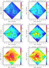 |
Fig. A.1 SPIRE-FTS surface brightness maps of the mid-J CO line emission. |
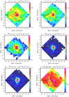 |
Fig. A.2 SPIRE-FTS surface brightness maps of CO, 13CO, and [C I] line emission. |
References
- Abel, N. P., Dudley, C., Fischer, J., Satyapal, S., & van Hoof, P. A. M. 2009, ApJ, 701, 1147 [NASA ADS] [CrossRef] [Google Scholar]
- Aladro, R., Martín, S., Riquelme, D., et al. 2015, A&A, 579, A101 [NASA ADS] [CrossRef] [EDP Sciences] [Google Scholar]
- Arab, H., Abergel, A., Habart, E., et al. 2012, A&A, 541, A19 [NASA ADS] [CrossRef] [EDP Sciences] [Google Scholar]
- Arendt, R. G., Staguhn, J., Dwek, E., et al. 2019, ApJ, 885, 71 [Google Scholar]
- Armijos-Abendaño, J., Banda-Barragán, W. E., Martín-Pintado, J., et al. 2020a, MNRAS, 499, 4918 [Google Scholar]
- Armijos-Abendaño, J., Martín-Pintado, J., López, E., et al. 2020b, ApJ, 895, 57 [Google Scholar]
- Benson, J. M., & Johnston, K. J. 1984, ApJ, 277, 181 [NASA ADS] [CrossRef] [Google Scholar]
- Bergin, E. A., & Tafalla, M. 2007, ARA&A, 45, 339 [NASA ADS] [CrossRef] [Google Scholar]
- Bernard, J. P., Paradis, D., Marshall, D. J., et al. 2010, A&A, 518, L88 [NASA ADS] [CrossRef] [EDP Sciences] [Google Scholar]
- Binney, J., Gerhard, O. E., Stark, A. A., Bally, J., & Uchida, K. I. 1991, MNRAS, 252, 210 [NASA ADS] [CrossRef] [Google Scholar]
- Bisbas, T. G., van Dishoeck, E. F., Papadopoulos, P. P., et al. 2017, ApJ, 839, 90 [NASA ADS] [CrossRef] [Google Scholar]
- Bohlin, R. C., Savage, B. D., & Drake, J. F. 1978, ApJ, 224, 132 [NASA ADS] [CrossRef] [Google Scholar]
- Bron, E., Agúndez, M., Goicoechea, J. R., & Cernicharo, J. 2018, ArXiv e-prints, unpublished [arXiv:1801.01547] [Google Scholar]
- Carey, S. J., Noriega-Crespo, A., Mizuno, D. R., et al. 2009, PASP, 121, 76 [NASA ADS] [CrossRef] [Google Scholar]
- Caselli, P., Benson, P. J., Myers, P. C., & Tafalla, M. 2002, ApJ, 572, 238 [NASA ADS] [CrossRef] [Google Scholar]
- Ceccarelli, C., Dominik, C., López-Sepulcre, A., et al. 2014, ApJ, 790, L1 [NASA ADS] [CrossRef] [Google Scholar]
- Cernicharo, J., Goicoechea, J. R., Pardo, J. R., & Asensio-Ramos, A. 2006, ApJ, 642, 940 [NASA ADS] [CrossRef] [Google Scholar]
- Clark, J. S., Lohr, M. E., Patrick, L. R., et al. 2018, A&A, 618, A2 [NASA ADS] [CrossRef] [EDP Sciences] [Google Scholar]
- Dent, W. R. F., Hovey, G. J., Dewdney, P. E., et al. 2009, MNRAS, 395, 1805 [NASA ADS] [CrossRef] [Google Scholar]
- Desert, F. X., Boulanger, F., & Puget, J. L. 1990, A&A, 500, 313 [Google Scholar]
- de Vicente, P., Martin-Pintado, J., & Wilson, T. L. 1997, A&A, 320, 957 [NASA ADS] [Google Scholar]
- Dowell, C. D., Lis, D. C., Serabyn, E., et al. 1999, ASP Conf. Ser., 186, 453 [Google Scholar]
- Dwarkadas, V. V. 2011, Mem. Soc. Astron. It., 82, 781 [NASA ADS] [Google Scholar]
- Dwek, E., & Arendt, R. G. 2020, ApJ, 901, 36 [CrossRef] [Google Scholar]
- Etxaluze, M., Goicoechea, J. R., Cernicharo, J., et al. 2013, A&A, 556, A137 [NASA ADS] [CrossRef] [EDP Sciences] [Google Scholar]
- Fischer, J., Sturm, E., González-Alfonso, E., et al. 2010, A&A, 518, L41 [NASA ADS] [CrossRef] [EDP Sciences] [Google Scholar]
- Flower, D. R., & Pineau des Forêts, G. 2010, MNRAS, 406, 1745 [Google Scholar]
- Fukui, Y., Habe, A., Inoue, T., Enokiya, R., & Tachihara, K. 2021, PASJ, 73, S1 [Google Scholar]
- Gahm, G. F., Persson, C. M., Mäkelä, M. M., & Haikala, L. K. 2013, A&A, 555, A57 [NASA ADS] [CrossRef] [EDP Sciences] [Google Scholar]
- Gaume, R. A., Claussen, M. J., de Pree, C. G., Goss, W. M., & Mehringer, D. M. 1995, ApJ, 449, 663 [NASA ADS] [CrossRef] [Google Scholar]
- Gerin, M., Neufeld, D. A., & Goicoechea, J. R. 2016, ARA&A, 54, 181 [NASA ADS] [CrossRef] [Google Scholar]
- Ginsburg, A., & Kruijssen, J. M. D. 2018, ApJ, 864, L17 [Google Scholar]
- Ginsburg, A., Bally, J., Barnes, A., et al. 2018, ApJ, 853, 171 [NASA ADS] [CrossRef] [Google Scholar]
- Goicoechea, J. R., Rodríguez-Fernández, N. J., & Cernicharo, J. 2004, ApJ, 600, 214 [NASA ADS] [CrossRef] [Google Scholar]
- Goicoechea, J. R., Cernicharo, J., Karska, A., et al. 2012, A&A, 548, A77 [NASA ADS] [CrossRef] [EDP Sciences] [Google Scholar]
- Goicoechea, J. R., Etxaluze, M., Cernicharo, J., et al. 2013, ApJ, 769, L13 [NASA ADS] [CrossRef] [Google Scholar]
- Goicoechea, J. R., Chavarría, L., Cernicharo, J., et al. 2015a, ApJ, 799, 102 [Google Scholar]
- Goicoechea, J. R., Teyssier, D., Etxaluze, M., et al. 2015b, ApJ, 812, 75 [NASA ADS] [CrossRef] [Google Scholar]
- Goicoechea, J. R., Pety, J., Cuadrado, S., et al. 2016, Nature, 537, 207 [NASA ADS] [CrossRef] [Google Scholar]
- Goicoechea, J. R., Santa-Maria, M. G., Teyssier, D., et al. 2018, A&A, 616, L1 [NASA ADS] [CrossRef] [EDP Sciences] [Google Scholar]
- Goicoechea, J. R., Santa-Maria, M. G., Bron, E., et al. 2019, A&A, 622, A91 [NASA ADS] [CrossRef] [EDP Sciences] [Google Scholar]
- Goicoechea, J. R., Pabst, C. H. M., Kabanovic, S., et al. 2020, A&A, 639, A1 [CrossRef] [EDP Sciences] [Google Scholar]
- Goldsmith, P. F., & Langer, W. D. 1999, ApJ, 517, 209 [Google Scholar]
- Goldsmith, P. F., Lis, D. C., Hills, R., & Lasenby, J. 1990, ApJ, 350, 186 [NASA ADS] [CrossRef] [Google Scholar]
- Goldsmith, P. F., Lis, D. C., Lester, D. F., & Harvey, P. M. 1992, ApJ, 389, 338 [NASA ADS] [CrossRef] [Google Scholar]
- González-Alfonso, E., Smith, H. A., Fischer, J., & Cernicharo, J. 2004, ApJ, 613, 247 [NASA ADS] [CrossRef] [Google Scholar]
- Goto, M., Usuda, T., Geballe, T. R., et al. 2011, PASJ, 63, L13 [NASA ADS] [CrossRef] [Google Scholar]
- Graciá-Carpio, J., Sturm, E., Hailey-Dunsheath, S., et al. 2011, ApJ, 728, L7 [NASA ADS] [CrossRef] [Google Scholar]
- Gravity Collaboration (Abuter, R., et al.) 2019, A&A, 625, L10 [NASA ADS] [CrossRef] [EDP Sciences] [Google Scholar]
- Greaves, J. S., & Williams, P. G. 1994, A&A, 290, 259 [NASA ADS] [Google Scholar]
- Griffin, M. J., Abergel, A., Abreu, A., et al. 2010, A&A, 518, L3 [EDP Sciences] [Google Scholar]
- Hacar, A., Alves, J., Tafalla, M., & Goicoechea, J. R. 2017, A&A, 602, L2 [NASA ADS] [CrossRef] [EDP Sciences] [Google Scholar]
- Hacar, A., Tafalla, M., Forbrich, J., et al. 2018, A&A, 610, A77 [NASA ADS] [CrossRef] [EDP Sciences] [Google Scholar]
- Hasegawa, T., Sato, F., Whiteoak, J. B., & Miyawaki, R. 1994, ApJ, 429, L77 [NASA ADS] [CrossRef] [Google Scholar]
- Hatchfield, H. P., Battersby, C., Keto, E., et al. 2020, ApJS, 251, 14 [Google Scholar]
- Henshaw, J. D., Longmore, S. N., Kruijssen, J. M. D., et al. 2016, MNRAS, 457, 2675 [NASA ADS] [CrossRef] [Google Scholar]
- Herbst, E., & Klemperer, W. 1973, ApJ, 185, 505 [NASA ADS] [CrossRef] [Google Scholar]
- Herrera-Camus, R., Sturm, E., Graciá-Carpio, J., et al. 2018, ApJ, 861, 95 [Google Scholar]
- H.E.S.S. Collaboration (Abramowski, A., et al.) 2016, Nature, 531, 476 [NASA ADS] [CrossRef] [PubMed] [Google Scholar]
- Hildebrand, R. H. 1983, QJRAS, 24, 267 [NASA ADS] [Google Scholar]
- Hirashita, H., Hibi, Y., & Shibai, H. 2007, MNRAS, 379, 974 [NASA ADS] [CrossRef] [Google Scholar]
- Hollenbach, D., & McKee, C. F. 1989, ApJ, 342, 306 [NASA ADS] [CrossRef] [Google Scholar]
- Hollenbach, D. J., & Tielens, A. G. G. M. 1999, Rev. Mod. Phys., 71, 173 [Google Scholar]
- Hosokawa, T., & Inutsuka, S.-i. 2006, ApJ, 646, 240 [NASA ADS] [CrossRef] [Google Scholar]
- Hüttemeister, S., Wilson, T. L., Henkel, C., & Mauersberger, R. 1993, A&A, 276, 445 [NASA ADS] [Google Scholar]
- Hüttemeister, S., Wilson, T. L., Mauersberger, R., et al. 1995, A&A, 294, 667 [NASA ADS] [Google Scholar]
- Indriolo, N., & McCall, B. J. 2012, ApJ, 745, 91 [NASA ADS] [CrossRef] [Google Scholar]
- Indriolo, N., Neufeld, D. A., Gerin, M., et al. 2015, ApJ, 800, 40 [NASA ADS] [CrossRef] [Google Scholar]
- Indriolo, N., Bergin, E. A., Goicoechea, J. R., et al. 2017, ApJ, 836, 117 [NASA ADS] [CrossRef] [Google Scholar]
- Jiménez-Serra, I., Caselli, P., Tan, J. C., et al. 2010, MNRAS, 406, 187 [NASA ADS] [CrossRef] [Google Scholar]
- Joblin, C., Bron, E., Pinto, C., et al. 2018, A&A, 615, A129 [NASA ADS] [CrossRef] [EDP Sciences] [Google Scholar]
- Johnson, C. T., Burke, P. G., & Kingston, A. E. 1987, J. Phys. B Atm. Mol. Phys., 20, 2553 [Google Scholar]
- Jones, P. A., Burton, M. G., Cunningham, M. R., et al. 2012, MNRAS, 419, 2961 [NASA ADS] [CrossRef] [Google Scholar]
- Kamenetzky, J., Rangwala, N., Glenn, J., Maloney, P. R., & Conley, A. 2014, ApJ, 795, 174 [NASA ADS] [CrossRef] [Google Scholar]
- Kauffmann, J., Bertoldi, F., Bourke, T. L., Evans, N. J., I., & Lee, C. W. 2008, A&A, 487, 993 [NASA ADS] [CrossRef] [EDP Sciences] [Google Scholar]
- Kirk, H., Myers, P. C., Bourke, T. L., et al. 2013, ApJ, 766, 115 [NASA ADS] [CrossRef] [Google Scholar]
- Koyama, K., Maeda, Y., Sonobe, T., et al. 1996, PASJ, 48, 249 [NASA ADS] [CrossRef] [Google Scholar]
- Langer, W. D., & Penzias, A. A. 1990, ApJ, 357, 477 [Google Scholar]
- Langer, W. D., Goldsmith, P. F., Pineda, J. L., et al. 2015, A&A, 576, A1 [NASA ADS] [CrossRef] [EDP Sciences] [Google Scholar]
- Le Bourlot J., Pineau des Forets, G., Roueff, E., & Schilke, P. 1993, ApJ, 416, L87 [NASA ADS] [CrossRef] [Google Scholar]
- Lee, M. Y., Madden, S. C., Le Petit, F., et al. 2019, A&A, 628, A113 [EDP Sciences] [Google Scholar]
- Lehmann, A., Godard, B., Pineau des Forêts, G., & Falgarone, E. 2020, A&A 643, A101 [EDP Sciences] [Google Scholar]
- Le Petit, F., Nehmé, C., Le Bourlot, J., & Roueff, E. 2006, ApJS, 164, 506 [NASA ADS] [CrossRef] [EDP Sciences] [Google Scholar]
- Le Petit, F., Ruaud, M., Bron, E., et al. 2016, A&A, 585, A105 [NASA ADS] [CrossRef] [EDP Sciences] [Google Scholar]
- Li, A., & Draine, B. T. 2001, ApJ, 554, 778 [Google Scholar]
- Lis, D. C., & Goldsmith, P. F. 1990, ApJ, 356, 195 [NASA ADS] [CrossRef] [Google Scholar]
- Luhman, M. L., Satyapal, S., Fischer, J., et al. 1998, ApJ, 504, L11 [NASA ADS] [CrossRef] [Google Scholar]
- Maeda, Y., Baganoff, F. K., Feigelson, E. D., et al. 2002, ApJ, 570, 671 [NASA ADS] [CrossRef] [Google Scholar]
- Malhotra, S., Kaufman, M. J., Hollenbach, D., et al. 2001, ApJ, 561, 766 [Google Scholar]
- Martin, A. H. M., & Downes, D. 1972, Astrophys. Lett., 11, 219 [Google Scholar]
- Martín, S., Mauersberger, R., Martín-Pintado, J., Henkel, C., & García-Burillo, S. 2006, ApJS, 164, 450 [NASA ADS] [CrossRef] [Google Scholar]
- Martín, S., Martín-Pintado, J., & Viti, S. 2009, ApJ, 706, 1323 [NASA ADS] [CrossRef] [Google Scholar]
- Martin-Pintado, J., Bachiller, R., & Fuente, A. 1992, A&A, 254, 315 [NASA ADS] [Google Scholar]
- Martín-Pintado, J., Gaume, R. A., Rodríguez-Fernández, N., de Vicente, P., & Wilson, T. L. 1999, ApJ, 519, 667 [NASA ADS] [CrossRef] [Google Scholar]
- Martín-Pintado, J., de Vicente, P., Rodríguez-Fernández, N. J., Fuente, A., & Planesas, P. 2000, A&A, 356, L5 [NASA ADS] [Google Scholar]
- Mashian, N., Sturm, E., Sternberg, A., et al. 2015, ApJ, 802, 81 [Google Scholar]
- Mauersberger, R., & Henkel, C. 1991, A&A, 245, 457 [NASA ADS] [Google Scholar]
- Mehringer, D. M., Yusef-Zadeh, F., Palmer, P., & Goss, W. M. 1992, ApJ, 401, 168 [NASA ADS] [CrossRef] [Google Scholar]
- Mehringer, D. M., Palmer, P., Goss, W. M., & Yusef-Zadeh, F. 1993, ApJ, 412, 684 [NASA ADS] [CrossRef] [Google Scholar]
- Meijerink, R., Kristensen, L. E., Weiß, A., et al. 2013, ApJ, 762, L16 [NASA ADS] [CrossRef] [Google Scholar]
- Meng, F., Sánchez-Monge, Á., Schilke, P., et al. 2019, A&A, 630, A73 [NASA ADS] [CrossRef] [EDP Sciences] [Google Scholar]
- Mikami, H., Umemoto, T., Yamamoto, S., & Saito, S. 1992, ApJ, 392, L87 [NASA ADS] [CrossRef] [Google Scholar]
- Miyazaki, A., & Tsuboi, M. 2000, ApJ, 536, 357 [NASA ADS] [CrossRef] [Google Scholar]
- Molinari, S., Swinyard, B., Bally, J., et al. 2010, PASP, 122, 314 [NASA ADS] [CrossRef] [Google Scholar]
- Molinari, S., Bally, J., Noriega-Crespo, A., et al. 2011, ApJ, 735, L33 [NASA ADS] [CrossRef] [Google Scholar]
- Morris, M., & Serabyn, E. 1996, ARA&A, 34, 645 [NASA ADS] [CrossRef] [Google Scholar]
- Murakami, H., Koyama, K., Sakano, M., Tsujimoto, M., & Maeda, Y. 2000, ApJ, 534, 283 [NASA ADS] [CrossRef] [Google Scholar]
- Neill, J. L., Bergin, E. A., Lis, D. C., et al. 2014, ApJ, 789, 8 [NASA ADS] [CrossRef] [Google Scholar]
- Neufeld, D. A., & Dalgarno, A. 1989, ApJ, 344, 251 [NASA ADS] [CrossRef] [Google Scholar]
- Nolan, P. L., Abdo, A. A., Ackermann, M., et al. 2012, ApJS, 199, 31 [NASA ADS] [CrossRef] [Google Scholar]
- Ott, S. 2010, ASP Conf. Ser., 434, 139 [Google Scholar]
- Pabst, C., Higgins, R., Goicoechea, J. R., et al. 2019, Nature, 565, 618 [NASA ADS] [CrossRef] [Google Scholar]
- Pabst, C. H. M., Goicoechea, J. R., Teyssier, D., et al. 2020, A&A, 639, A2 [CrossRef] [EDP Sciences] [Google Scholar]
- Padovani, M., Marcowith, A., Sánchez-Monge, Á., Meng, F., & Schilke, P. 2019, A&A, 630, A72 [NASA ADS] [CrossRef] [EDP Sciences] [Google Scholar]
- Padovani, M., Ivlev, A. V., Galli, D., et al. 2020, Space Sci. Rev., 216, 29 [Google Scholar]
- Pérez-Beaupuits, J. P., Güsten, R., Harris, A., et al. 2018, ApJ, 860, 23 [CrossRef] [Google Scholar]
- Pety, J., Guzmán, V. V., Orkisz, J. H., et al. 2017, A&A, 599, A98 [NASA ADS] [CrossRef] [EDP Sciences] [Google Scholar]
- Pilbratt, G. L., Riedinger, J. R., Passvogel, T., et al. 2010, A&A, 518, L1 [CrossRef] [EDP Sciences] [Google Scholar]
- Pineau des Forêts, G., Roueff, E., & Flower, D. R. 1992, MNRAS, 258, 45P [NASA ADS] [CrossRef] [Google Scholar]
- Rangwala, N., Maloney, P. R., Glenn, J., et al. 2011, ApJ, 743, 94 [NASA ADS] [CrossRef] [Google Scholar]
- Revnivtsev, M. G., Churazov, E. M., Sazonov, S. Y., et al. 2004, A&A, 425, L49 [NASA ADS] [CrossRef] [EDP Sciences] [Google Scholar]
- Rigopoulou, D., Hurley, P. D., Swinyard, B. M., et al. 2013, MNRAS, 434, 2051 [Google Scholar]
- Rodríguez-Fernández, N. J., Tafalla, M., Gueth, F., & Bachiller, R. 2010, A&A, 516, A98 [NASA ADS] [CrossRef] [EDP Sciences] [Google Scholar]
- Röllig, M., Simon, R., Güsten, R., et al. 2016, A&A, 591, A33 [NASA ADS] [CrossRef] [EDP Sciences] [Google Scholar]
- Rosenberg, M. J. F., van der Werf, P. P., Aalto, S., et al. 2015, ApJ, 801, 72 [NASA ADS] [CrossRef] [Google Scholar]
- Salgado, F., Berné, O., Adams, J. D., et al. 2016, ApJ, 830, 118 [NASA ADS] [CrossRef] [Google Scholar]
- Sanders, D. B., & Mirabel, I. F. 1996, ARA&A, 34, 749 [NASA ADS] [CrossRef] [Google Scholar]
- Sanhueza, P., Jackson, J. M., Foster, J. B., et al. 2012, ApJ, 756, 60 [NASA ADS] [CrossRef] [Google Scholar]
- Sato, F., Hasegawa, T., Whiteoak, J. B., & Miyawaki, R. 2000, ApJ, 535, 857 [NASA ADS] [CrossRef] [Google Scholar]
- Schinnerer, E., Meidt, S. E., Pety, J., et al. 2013, ApJ, 779, 42 [NASA ADS] [CrossRef] [Google Scholar]
- Schirm, M. R. P., Wilson, C. D., Parkin, T. J., et al. 2014, ApJ, 781, 101 [Google Scholar]
- Schmiedeke, A., Schilke, P., Möller, T., et al. 2016, A&A, 588, A143 [NASA ADS] [CrossRef] [EDP Sciences] [Google Scholar]
- Schroder, K., Staemmler, V., Smith, M. D., Flower, D. R., & Jaquet, R. 1991, J. Phys. B Atm. Mol. Phys., 24, 2487 [NASA ADS] [CrossRef] [Google Scholar]
- Schultheis, M., Ganesh, S., Simon, G., et al. 1999, A&A, 349, L69 [NASA ADS] [Google Scholar]
- Swinyard, B. M., Polehampton, E. T., Hopwood, R., et al. 2014, MNRAS, 440, 3658 [Google Scholar]
- Takano, S., Nakajima, T., & Kohno, K. 2019, PASJ, 71, S20 [Google Scholar]
- Taniguchi, A. 2019, astropenguin/ndradex [Google Scholar]
- Tauber, J. A.,& Goldsmith, P. F. 1990, ApJ, 356, L63 [Google Scholar]
- Tauber, J. A., Lis, D. C., Keene, J., Schilke, P., & Buettgenbach, T. H. 1995, A&A, 297, 567 [Google Scholar]
- Tayal, S. S. 2011, ApJS, 195, 12 [NASA ADS] [CrossRef] [Google Scholar]
- Terrier, R., Ponti, G., Bélanger, G., et al. 2010, ApJ, 719, 143 [Google Scholar]
- Terrier, R., Clavel, M., Soldi, S., et al. 2018, A&A, 612, A102 [NASA ADS] [CrossRef] [EDP Sciences] [Google Scholar]
- Thiel, V., Belloche, A., Menten, K. M., et al. 2019, A&A, 623, A68 [NASA ADS] [CrossRef] [EDP Sciences] [Google Scholar]
- Tielens, A. G. G. M., & Hollenbach, D. 1985, ApJ, 291, 722 [Google Scholar]
- Tsuboi, M., Miyazaki, A., & Uehara, K. 2015, PASJ, 67, 109 [NASA ADS] [Google Scholar]
- Valinia, A., Tatischeff, V., Arnaud, K., Ebisawa, K., & Ramaty, R. 2000, ApJ, 543, 733 [NASA ADS] [CrossRef] [Google Scholar]
- van der Tak, F. F. S., Black, J. H., Schöier, F. L., Jansen, D. J., & van Dishoeck, E. F. 2007, A&A, 468, 627 [NASA ADS] [CrossRef] [EDP Sciences] [Google Scholar]
- van der Werf, P. P., Isaak, K. G., Meijerink, R., et al. 2010, A&A, 518, L42 [NASA ADS] [CrossRef] [EDP Sciences] [Google Scholar]
- Whiteoak, J. B., & Gardner, F. F. 1983, MNRAS, 205, 27P [Google Scholar]
- Wu, R., Bron, E., Onaka, T., et al. 2018, A&A, 618, A53 [NASA ADS] [CrossRef] [EDP Sciences] [Google Scholar]
- Yang, B., Stancil, P. C., Balakrishnan, N., & Forrey, R. C. 2010, ApJ, 718, 1062 [NASA ADS] [CrossRef] [Google Scholar]
- Yusef-Zadeh, F., Hewitt, J. W., Arendt, R. G., et al. 2009, ApJ, 702, 178 [NASA ADS] [CrossRef] [Google Scholar]
- Yusef-Zadeh, F., Hewitt, J. W., Wardle, M., et al. 2013, ApJ, 762, 33 [NASA ADS] [CrossRef] [Google Scholar]
- Zhang, S., Hailey, C. J., Mori, K., et al. 2015, ApJ, 815, 132 [NASA ADS] [CrossRef] [Google Scholar]
Nonionizing far-UV (FUV) photons have energies hν < 13.6 eV and extreme-UV (EUV) ionizing photons have energies hν > 13.6 eV.
The [C I] 809 GHz and CO J = 7−6 lines are blended in the apodized FTS spectra, but not in the unapodized spectra. We independently extracted their integrated line intensities from the unapodized spectra.
We use the Spearman’s correlation, instead of the usual Pearson’s correlation, because the molecular emission is not normally distributed. Spearman’s correlation is a non parametric statistic which measures the monotonic relationship. A ρ = 0 does not imply that there is no relationship between the variables, just that it is not monotonic.
We define the standard deviation or dispersion of the dust temperature as: σ =  .
.
We considered CO –H2, C –H2, and C –e inelastic collision rate coefficients of Yang et al. (2010), Schroder et al. (1991), and Johnson et al. (1987), respectively. The model assumes that the H2 ortho-to-para ratio is thermalized to Tk. We checked that C –e collisions do not start to contribute to the [C I] excitation unless the ionization fraction (the electron abundance xe = ne / nH) is unrealistically high, xe > 10−2.
We define the rms value of each model fit as
rms2 =
 , where N is the number of lines,
  is the observed intensity, and
  that of the model.
The [C I]-emitting gas in Sgr B2 is much denser than the warm (Tk ≃ 200−500 K) and diffuse clouds (nH ≲ 100 cm−3) invoked to explain the presence of absorption lines from excited metastable levels of H (e.g., Goto et al. 2011). These diffuse clouds in the CMZ typically absorb at negative LSR velocities and have higher ζCR rates (≳ 10−14 s−1, e.g., Indriolo et al. 2015; Le Petit et al. 2016). The different ζCR values likely imply that ζCR decreases for increasing depths inside dense clouds.
Our best models of the [C I] emission belong to the HIP category. They lead to xe ≳ 5 × 10⁻⁵ and high N(C)/N(CO) and N(C)/N(C+) ratios.
We add the CO line intensities from Ju ≥ 4 only, but we note that in warm gas, the low-J CO lines have a very modest contribution to the total CO surface brightness in W m−2 sr−1 units.
All Tables
Summary of FIR- and submm-related magnitudes that are spatially correlated in the mapped area of Sgr B2.
Warm CO and C excitation temperatures and column densities derived from population diagrams toward the reference positions.
All Figures
|
Fig. 1 RGB view of about half of the CMZ (~50′ × 60′) in the GC. Red: SPIRE 350 μm tracing cold dust from the most prominent molecular clouds. Green: PACS 70 μm tracing warm dust, mostly in extended PDR-like environments. Blue: MIPS 24 μm tracing hot dust, mostly from ionized regions. The rhombus marks the ~13′ × 13′ area mapped with SPIRE-FTS around Sgr B2(M,N) massive star-forming cores. |
| In the text | |
|
Fig. 2 Selection of SPIRE-FTS integrated line intensity maps. The map center coordinates are those of Sgr B2(M) core: RA, Dec = 17h 47m 20.5s, −28° 23′ 06′′. Black stars mark the location of the three massive star-forming cores Sgr B2(N, M, and S). Black triangles mark other H II regions (Mehringer et al. 1992, 1993; Meng et al. 2019). The black dashed circle of radius 2.5′ (~5.0 pc), centered at RA, Dec = 17h 47m 39.7s, −28° 25′ 48′′ marks a specific X-ray irradiated region (Zhang et al. 2015). The pink dashed circles in panel a show Shells 1, 2, and 3 of Tsuboi et al. (2015). White circles show positions A, B, C, and D. |
| In the text | |
|
Fig. 3 SPIRE-FTS continuum-divided spectra toward four representative positions of Sgr B2 envelope: A in black, B in blue, C in magenta, and D in cyan (the Iν ∕Icont scale appliesto the C spectrum, all the others are shifted). The D spectrum is unapodized, the other three are apodized. |
| In the text | |
|
Fig. 4 Total integrated line intensity maps (in units K km s−1) of different molecular lines observed with the IRAM 30 m telescope toward the Sgr B2 molecular complex and integrated in the LSR velocity range [ − 20, 120] km s−1. The gray dashed circle marks a specific X-ray irradiated region (Zhang et al. 2015). The pink dashed circles show Shells 1, 2, and 3 of Tsuboi et al. (2015). |
| In the text | |
|
Fig. 5 IRAM30 m maps of the N2H+ (1−0) and SiO (2−1) line intensities integrated in the 15−50 km s−1 and 50−85 km s−1 ranges. Contours in panels a and c represent the 2015 hard X-ray emission integrated from 3 to 79 keV (Zhang et al. 2015). Gray: 19 × 10−6 ph s−1 pixel−1. Cyan: 22 × 10−6 ph s−1 pixel−1. Red: (24, 26, 28) ×10−6 ph s−1 pixel−1. Dashed white lines delineate the regions with no X-ray observations. Contours in panels b and d represent the 350 μm emission from 8 to 68 by 20 (103) MJy sr−1. |
| In the text | |
|
Fig. 6 IRAM30 m maps of the HCO+ (1−0) and HCN (1−0) line intensities integrated in the 15−50 km s−1 and 50−85 km s−1 ranges. Contours in panels a and c represent the hard X-Rays emission integrated from 3 to 79 keV, using the 2015 NuSTAR data (Zhang et al. 2015). Gray: 19 × 10−6 ph s−1 pixel−1. Cyan: 22 × 10−6 ph s−1 pixel−1. Red: (24, 26, 28) ×10−6 ph s−1 pixel−1. Dashed white lines delineate the regions with no X-ray observations. Contours inpanels b and d represent the 350 μm data from 8 to 68 by 20 (× 103) MJy sr−1. |
| In the text | |
|
Fig. 7 HCN (1−0), HCO+ (1−0), SiO (2−1), and N2H+ (1−0) line profiles toward positions D, A, B, and C. The vertical dashed line at vLSR = 50 km s−1 marks a representative velocity of Sgr B2 envelope. |
| In the text | |
|
Fig. 8 Dust continuum emission at different wavelengths. (a) MIPS 24 μm (VSGs), (b) PACS 70 μm, (c) SPIRE 350 μm, and (d) R% = I24 / I70 × 100 ratio. Black stars mark the location of the massive star-forming cores N, M, and S. Black triangles mark other H II regions (Mehringer et al. 1992, 1993; Meng et al. 2019). The dashed circle marks a specific X-ray irradiated region (Zhang et al. 2015). |
| In the text | |
|
Fig. 9 Dust emission: MIPS 24 μm, HiGAL 70, 250, 350, and 500 μm photometric data, all convolved to 42″ resolution (squares, with an intensity uncertainty of ≲15%). Continuous curves show the best-fit BG SEDs of representative positions A, B, C, and D. The 24 μm emissionis produced by hotter VSGs. The area below the continuous curves (40–500 μm) is the integrated FIR intensity (IFIR). |
| In the text | |
|
Fig. 10 Dust emission properties. (a) Dust temperature derived from SED fist to the photometric data. Contours represent the [N II] 205 μm data. Black: 6 × 10⁻⁸ W m−2 sr−1, gray: 8.5 × 10⁻⁸ W m−2 sr−1, and red: 12 × 10−8 W m−2 sr−1. (b) Map of the dust opacity at 350 μm. (c) Spatial distribution of the molecular gas column density N(H2). (d) Far-IR surface brightness map integrated from 40 to 500 μm. All these maps have a uniform angular resolution of 42′′. |
| In the text | |
|
Fig. 11 Map of the FIR-luminosity to gas-mass ratio LFIR / Mgas in units of L⊙ / M⊙ per pixel (at an angular resolution of 42″). Contours represent 24 μm emission levels from 3 × 10⁴ MJy sr−1 (red) to 200 MJy sr−1 (blue). |
| In the text | |
|
Fig. 12 Maps of Tex for (a) atomic carbon and (c) mid-J CO. Contours represent the 13CO J = 5−4 emission from 10−9 W m−2 sr−1 (gray) to 2.8 × 10⁻⁸ W m−2 sr−1 (magenta) tracing high N(H2) regions. (b) Line surface brightness 12CO / 13CO J = 5−4 ratio map. (d) Population diagrams of 12CO lines observed with SPIRE-FTS toward positions A, B, C, and D in Sgr B2 (see Table 4). Dashed curves refer to fits to positions A and D. |
| In the text | |
|
Fig. 13 Maps of N(C) and N(warm CO) derived from the population diagram analysis. (a) Contours represent the hard X-Rays integrated from 3 to 79 keV, using the 2015 NuSTAR data (Zhang et al. 2015). Red: (22, 24, 26, 28) ×10−6 ph s−1 pixel−1. Blue: 19 × 10−6 ph s−1 pixel−1. The regions inside the white dashed contours are those of no exposures. |
| In the text | |
|
Fig. 14 Maps of Pth/k derived fromsingle-slab non-LTE excitation models applied to mid-J CO (upper panel) and [C I] lines (lower panel). |
| In the text | |
|
Fig. 15 Observed mid-J CO (left panel) and [C I] line intensities (right panel) toward positions A, B, C, and D (shown as triangles). Observed CO and [C I] lines have an intensity uncertainty of ~20%. Continuous curves show predictions from PDR models with different values of G0 and nH (in units of cm−3). Dashed curves in the left panel show C-type shock modelpredictions (from Flower & Pineau Des Forêts 2010). |
| In the text | |
|
Fig. 16 Abundance, line emissivity, and Tk profiles of PDR models with G0 = 103 and ζCR = 2 × 10⁻¹⁵ s−1, consistent with the observed [C I] emission (nH = 103 cm−3; left) and the mid-J CO emission (nH = 106 cm−3; right). We note the different spatial scales (upper axis). |
| In the text | |
|
Fig. 17 Model predictions for different values of ζCR (and fixed G0 = 103, nH = 105, 106 cm−3, and AV, tot = 15 mag). Continuous curves show the column density enhancement N∕N0 with respect to the models with ζCR,0 = 2 × 10⁻¹⁷ s−1 (roughly theionization rate in disk GMCs). |
| In the text | |
|
Fig. 18 CO to FIR intensity ratio. Contours represent the hard X-ray emission using the 2015 NuSTAR data (S. Zhang priv. comm.; no data inside the areas enclosed by the white dashed lines). Red: (22, 24, 26, 28) ×10−6 ph s−1 pixel−1. Blue: 19 × 10−6 ph s−1 pixel−1. |
| In the text | |
|
Fig. 19 Spatial distribution of the [C I] (492 + 809 GHz) and [NII] 205 μm to FIR intensity ratios in the Sgr B2. (a) Contours represent the hard X-ray emission integrated from 3 to 79 keV, using the 2015 NuSTAR data (same as in Fig. 18). (b) Contours represent the SPIRE 350 μm dust emission. |
| In the text | |
|
Fig. A.1 SPIRE-FTS surface brightness maps of the mid-J CO line emission. |
| In the text | |
|
Fig. A.2 SPIRE-FTS surface brightness maps of CO, 13CO, and [C I] line emission. |
| In the text | |
Current usage metrics show cumulative count of Article Views (full-text article views including HTML views, PDF and ePub downloads, according to the available data) and Abstracts Views on Vision4Press platform.
Data correspond to usage on the plateform after 2015. The current usage metrics is available 48-96 hours after online publication and is updated daily on week days.
Initial download of the metrics may take a while.