| Issue |
A&A
Volume 649, May 2021
|
|
|---|---|---|
| Article Number | A113 | |
| Number of page(s) | 16 | |
| Section | Interstellar and circumstellar matter | |
| DOI | https://doi.org/10.1051/0004-6361/202040106 | |
| Published online | 24 May 2021 | |
Fragmentation and kinematics in high-mass star formation
CORE-extension targeting two very young high-mass star-forming regions★
1
Max Planck Institute for Astronomy,
Königstuhl 17,
69117
Heidelberg,
Germany
e-mail: This email address is being protected from spambots. You need JavaScript enabled to view it.
2
UK Astronomy Technology Centre, Royal Observatory Edinburgh,
Blackford Hill,
Edinburgh
EH9 3HJ, UK
3
IRAM, 300 rue de la Piscine, Domaine Universitaire de Grenoble,
38406
St.-Martin-d’Hères, France
4
Centre for Astrophysics and Planetary Science, University of Kent,
Canterbury,
CT2 7NH, UK
5
Chinese Academy of Sciences Key Laboratory of FAST, National Astronomical Observatory of Cina,
Datun Road 20,
Chaoyang,
Bejing
100012, PR China
6
I. Physikalisches Institut, Universität zu Köln,
Zülpicher Str. 77,
50937
Köln, Germany
7
INAF, Osservatorio Astrofisico di Arcetri,
Largo E. Fermi 5,
50125
Firenze, Italy
8
Astrophysics Research Institute, Liverpool John Moores University,
146 Brownlow Hill,
Liverpool
L3 5RF, UK
9
Max-Planck-Institut für Astrophysik,
Karl-Schwarzschild-Str. 1,
85748
Garching, Germany
10
Instituto de Radioastronomıa y Astrofısica, Universidad Nacional Autonoma de Mexico,
PO Box 3-72,
58090
Morelia,
Michoacan, Mexico
11
School of Physics & Astronomy, E.C. Stoner Building, The University of Leeds,
Leeds
LS2 9JT, UK
12
Department of Physics and Astronomy, McMaster University,
1280 Main St. W,
Hamilton,
ON
L8S 4M1, Canada
13
Max-Planck-Institut für Radioastronomie,
Auf dem Hügel 69,
53121
Bonn, Germany
14
Institute of Astronomy and Astrophysics, University of Tübingen,
Auf der Morgenstelle 10,
72076
Tübingen, Germany
15
Leiden Observatory, Leiden University,
PO Box 9513,
2300
RA Leiden, The Netherlands
Received:
10
December
2020
Accepted:
26
February
2021
Abstract
Context. The formation of high-mass star-forming regions from their parental gas cloud and the subsequent fragmentation processes lie at the heart of star formation research.
Aims. We aim to study the dynamical and fragmentation properties at very early evolutionary stages of high-mass star formation.
Methods. Employing the NOrthern Extended Millimeter Array and the IRAM 30 m telescope, we observed two young high-mass star-forming regions, ISOSS22478 and ISOSS23053, in the 1.3 mm continuum and spectral line emission at a high angular resolution (~0.8″).
Results. We resolved 29 cores that are mostly located along filament-like structures. Depending on the temperature assumption, these cores follow a mass-size relation of approximately M ∝ r2.0 ± 0.3, corresponding to constant mean column densities. However, with different temperature assumptions, a steeper mass-size relation up to M ∝ r3.0 ± 0.2, which would be more likely to correspond to constant mean volume densities, cannot be ruled out. The correlation of the core masses with their nearest neighbor separations is consistent with thermal Jeans fragmentation. We found hardly any core separations at the spatial resolution limit, indicating that the data resolve the large-scale fragmentation well. Although the kinematics of the two regions appear very different at first sight – multiple velocity components along filaments in ISOSS22478 versus a steep velocity gradient of more than 50 km s−1 pc−1 in ISOSS23053 – the findings can all be explained within the framework of a dynamical cloud collapse scenario.
Conclusions. While our data are consistent with a dynamical cloud collapse scenario and subsequent thermal Jeans fragmentation, the importance of additional environmental properties, such as the magnetization of the gas or external shocks triggering converging gas flows, is nonetheless not as well constrained and would require future investigation.
Key words: stars: formation / ISM: clouds / ISM: kinematics and dynamics / stars: massive / stars: protostars
Data are only available at the CDS via anonymous ftp to cdsarc.u-strasbg.fr (130.79.128.5) or via http://cdsarc.u-strasbg.fr/viz-bin/cat/J/A+A/649/A113
© H. Beuther et al. 2021
 Open Access article, published by EDP Sciences, under the terms of the Creative Commons Attribution License (https://creativecommons.org/licenses/by/4.0), which permits unrestricted use, distribution, and reproduction in any medium, provided the original work is properly cited.
Open Access funding provided by Max Planck Society.
1 Introduction
During the hierarchical process of star formation, the gas has to flow from the large cloud scales down to the smallest scales, where disks and protostars form. While questions regarding the small-scale structure and the presence of disks toward more evolved high-mass protostellar objects have been subject to intense study for several decades (e.g., Cesaroni et al. 2007; Beltrán & de Wit 2016; Beuther et al. 2018), the earliest evolutionary stages of collapse and fragmentation during the formation processes of high-mass stars have not been investigated in depth thus far. This is in part related to the short evolutionary time-scales of early massive star formation (e.g., Beuther et al. 2007; Zinnecker & Yorke 2007; Tan et al. 2014) and the fact that hardly any high-mass starless core candidates manage to survive further scrutiny when additional star formation indicators become detected (e.g., Motte et al. 2007; Tan et al. 2016; Feng et al. 2016). A few exceptional regions exist that have remained starless even with high-resolution millimeter interferometric observations (e.g., G11.92 Cyganowski et al. 2014, 2017; IRDC18310-4 Beuther et al. 2013, 2015a; W43-MM1 Nony et al. 2018). However, at least the latter two examples are at comparably large distances of 3.4 and 4.9 kpc, respectively, reducing the ability to investigate structures at small physical spatial scales. Furthermore, recent investigations with the Atacama Large Millimeter Array (ALMA) and the Submillimeter Array (SMA) also started to further dissect samples of very young high-mass star-forming regions (e.g., Sanhueza et al. 2019; Svoboda et al. 2019; Li et al. 2019, 2020a). Important questions regarding the earliest evolutionary stages of high-mass star formation are related to the fragmentation properties of the dense gas and the associated kinematic properties. For example, we consider whether these very young regions fragment early on into many lower-mass cores that may then competitively accrete gas from the surrounding envelope (e.g., Bonnell et al. 2007; Smith et al. 2009). Alternatively, they may fragment into more massive cores with potentially less low-mass cores early on (e.g., Tan et al. 2014; Zhang et al. 2015; Csengeri et al. 2017; Beuther et al. 2018)? We ask how important filamentary accretion processes are (e.g., Schneider et al. 2010; Peretto et al. 2014; André et al. 2014; Chira et al. 2018; Hennebelle 2018; Padoan et al. 2020) and what the relative importance is of cloud-scale gravo-turbulent or thermal fragmentation versus fragmentation of the gravitationally unstable accretion flows for the star formation process (e.g., Peters et al. 2010)? Furthermore, it has been argued that high-mass star formation starts and proceeds in turbulent gas clumps (e.g., McKee & Tan 2003). However, recent high-spatial-resolution studies of a few very young high-mass star-forming have regions revealed that at high enough spatial and spectral resolution, the spectral lines resolve into multiple components, each with line widths that are nearly consistent with thermal line broadening (e.g., Beuther et al. 2015a; Hacar et al. 2018; Li et al. 2020b). Therefore, it may well be the case that the individual cores do not have turbulent properties but it is, rather, only the superposition of many of these individual cores and spectral components mimicking the broader lines that are typically seen with single-dish telescopes at lower spatial resolution (e.g., Smith et al. 2013; Hacar et al. 2017a). At a somewhat coarser resolution of >10 000 au, similar results indicating sub-sonic non-thermal motions were also found by Ragan et al. (2015) and Sokolov et al. (2018) in lower-density lines of N2 H+ and NH3, respectively.
With the goal of studying the kinematic and fragmentation properties at the onset of high-mass star formation, we employ highspatial resolution and high-density tracer observations at mm wavelengths toward two regions at very early evolutionary stages. The targets are part of the IRAM NOrthern Extended Millimeter Array (NOEMA) large program CORE aimed at studying the fragmentation, disk properties, kinematics, and chemistry during the formation of high-mass stars (Beuther et al. 2018). In the following, we summarize the main aspects of the CORE program.
2 The CORE and CORE-extension projects
With the goal to study the fragmentation, disk, outflow, and chemical properties of high-mass star formation, we have embarked on the NOEMA large program CORE, which observes 20 high-mass star-forming regions at a high spatial resolution (0.3″−0.4″) in the 1.3 mm line and continuum emission. The sample was selected based on being mainly in the evolutionary stage of high-mass protostellar objects (HMPOs), also known as MYSOs (massive young stellar objects). An overview and more details about the program can be found in Beuther et al. (2018)1.
To broaden the scope of CORE to even younger evolutionary stages, we conducted the CORE-extension part of the project, observing two much younger regions (ISOSS22478 and ISOSS23053) also at high spatial resolution and with a similar spectral setup. The goal of this CORE-extension is to investigate earlier evolutionary stages with a particular focus on the gas dynamics and chemical properties at the onset of high-mass star formation. Selection criteria for their youth were mainly their low temperatures and luminosities as well as the low luminosity-to-mass ratios L∕M (~0.4 and ~2.2 for ISOSS22478 and ISOSS2305, respectively). These L∕M ratios are typically more than an order of magnitude below those of the original CORE sample (Beuther et al. 2018). Below, we introduce the target regions and Sect. 2.2 presents the technical details of the CORE-extension project.
2.1 Target regions
While the main part of the program targets 20 HMPOs with already embedded massive young stellar objects, we also observed two younger regions in slightly more extended mosaics to investigate the earliest formation processes. These two regions were originally identified via the ISO Serendipity Survey (ISOSS), which observed the sky serendipitously also during slew times with the Infrared Space Observatory (ISO) at 170 μm (Bogun et al. 1996; Krause et al. 2004). Since the regions are located in the outer Galaxy, and not in front of strong Milky Way background emission, they do not appear as infrared dark clouds (IRDCs). However, their general physical properties put them in a similarly young evolutionary stage as typical IRDCs.
ISOSS22478+6357
Earlier studies of this region were conducted by Hennemann et al. (2008), Ragan et al. (2012) and Bihr et al. (2015). At a distance of ~3.23 kpc, the region has a mass reservoir of ~140 M⊙, placing it inthe category of intermediate-mass star-forming regions. The average temperatures based on NH3 and dust observations are between ~13 and ~21 K, and the region still has a low total luminosity of ~55 L⊙ (Ragan et al. 2012; Bihr et al. 2015). Figure 1 (left panel) gives a large-scale overview of the region comprising the Herschel 70 μm emission and the SCUBA 450 μm data (Ragan et al. 2012; Di Francesco et al. 2008).
ISOSS23053+5953
This region has also previously been investigated, for example, by Birkmann et al. (2007), Ragan et al. (2012) and Bihr et al. (2015). At a distance of ~4.31 kpc, the region has a mass reservoir and luminosity of 610 M⊙ and 1313 L⊙, respectively. Average NH3 and dust temperature for the region are ~18 and ~22 K (Bihr et al. 2015; Ragan et al. 2012). Figure 1 (right panel) shows the corresponding large-scale overview image of the region. While early studies already showed signatures of infall (Birkmann et al. 2007), an analysis of the kinematics of this region based on VLA (Very Large Array) NH3 observationsrevealed indications of two velocity components that may collide at the positions of the central cores (Bihr et al. 2015).
2.2 The CORE-extension technical setup
While the original CORE program utilized the old receiver and backend system with only a ~4 GHz wide band in a single sideband between 217.167 and 220.834 GHz, the upgraded NOEMA now allows us to use, in dual-polarization, a much broader bandwidth in the double-sideband mode with 7.8 GHz in each sideband. Specifically, we are covering the frequency ranges from ~213.3 to ~221.1 GHz as well as from ~228.8 to ~236.6 GHz. This spectral setup covers a multitude of strong spectral lines from many important molecules, for instance, deuterated species such as DCO+, DNC, or N2 D+, the temperature tracers H2CO or CH3CN, CO, and its isotopologues 13CO and C18O, shock tracers like SiO or larger molecules such as CH3OH or HCCCH. While the entire bandpass is covered at low spectral resolution (2 MHz corresponding to ~2.7 km s−1 at 220 GHz), all important lines are also covered by separate high-spectral-resolution units (0.06 MHz corresponding to ~0.08 km s−1 at 220 GHz).
More details about the spectral setup and the chemical properties of the regions will be given in a future paper by Gieser et al. (in prep.). Here, we focus on the dynamical properties and potential gas flows in these two regions.
3 Observations and data
The two regions were observed with NOEMA in February and March 2019 with ten antennas in the A, C, and D configurations covering baseline lengths roughly between 18 and 774 m. The sources ISOSS22478 and ISOSS23053 were observed as six-field and four-field mosaics, respectively (see red circles in Fig. 1). The phase centers and velocities of rest vlsr were RA (J2000.) 22:47:49.22994, Dec 63:56:45.2796 (Gal. long./lat. 109.86/4.26 degs) and vlsr = −39.7 km s−1 for ISOSS22478 and RA (J2000.) 23:05:22.46953, Dec 59:53:52.6192 (Gal. long./lat. 109.99/-0.28 degs) and vlsr = −51.7 km s−1 for ISOSS23053. Flux and bandpass calibration were conducted for both regions with MWC349 and 3c454.3, respectively. Regularly interleaved observations of nearby quasars were used for phase and amplitude calibration, namely, 0016+731 for ISOSS22078and J2223+628 for ISOSS23053.
Calibration and imaging of the data was performed with the CLIC and MAPPING software of the GILDAS package2. To achieve optimal imaging quality for these mosaics, we applied natural weighting during the imaging process. To create the continuum data, only the line-free parts of the spectrum were used. Since the regions are comparably line-poor, only small parts of the entire bandpass (Sect. 2.2) had to be excluded. Specifically, we excluded 280 MHz and 1800 MHz of the entire bandpass of ~15 600 MHz for ISOSS22478 and ISOSS23053, respectively. For the 1.3 mm continuum data, this resulted in synthesized beams of 0.92″ × 0.73″ (PA 51 deg) and 0.84″ × 0.74″ (PA 67 deg)for ISOSS22478 and ISOSS23053, respectively. This corresponds to approximate linear resolution elements of ~2700 and ~3500 au, respectively. The corresponding 1σ continuum rms values are 0.057 mJy beam−1 and 0.16 mJy beam−1, respectively. The absolute flux scale is estimated to be correct within 20%.
For the spectral line data, we obtained complementary single-dish observations with the IRAM 30 m telescope to compensate for the missing short spacings. These 30 m observations were conducted in the on-the-fly mode typically achieving rms values of ~0.1 K (Tmb).
The NOEMA and 30 m data were then combined in the imaging process with the task UV_SHORT, and we present the merged data for DCO+(3–2), SiO(5–4) and several H2CO lines at a spectral resolution of 0.3 km s−1. Again, natural weighting was applied, and the final 1σ rms and synthesized beam values are presented in Table 1. The other spectral lines and a detailed chemical analysis of the regions will be presented in Gieser et al. (in prep.).
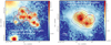 |
Fig. 1 Overview of the ISOSS22478+6357 (left) and ISOSS23053 (right) regions. The color scales and contours show the 70 and 450 μm emission from Herschel and SCUBA, respectively (Ragan et al. 2012; Di Francesco et al. 2008). The contour levels are from 18 to 98% of the peak emission of 1.88 and 14.88 Jy beam−1 for the two regions, respectively. Linear scale bars are shown and the red circles outline the NOEMA mosaics with a primary beam FWHM of 22″. |
4 Results
4.1 Fragmentation and continuum emission
To investigate the fragmentation properties of the large-scale gas clumps visible in Fig. 1, we showthe 1.3 mm dust continuum emission of the NOEMA data at a spatial resolution of ~0.8″ (Table 1) in Fig. 2. Both regions clearly fragment into numerous cores. Because we have no short spacing information for the continuum emission, these cores appear to be separated from each other. As we go on to see in the spectral line data discussed below (Sect. 4.2), these cores are neverthelessconnected by filamentary gas structures. Furthermore, we find that all cores are associated with 70 μm emission, hence, none of them are genuinely starless any longer.
Although the number of cores is not excessively large, to systematically derive the flux densities, offsets and sizes of the cores, we use the CLUMPFIND algorithm originally introduced by Williams et al. (1994). As a low-intensity threshold, we used the 5σ contours presented inFig. 3. We identify 15 and 14 cores for ISOSS22478 and ISOSS23053, respectively. Peak flux densities Speak, integrated fluxes S, RA and Dec, offset positions (Δx, Δy) and equivalent core radii are presented in Table 2. The equivalent core radii are calculated from the measured core area assuming a spherical distribution. No deconvolution from the synthesized beam was applied.
Core masses and peak column densities can be estimated from the integrated fluxes, S, and the peak flux densities, Speak, assuming optically thin dust continuum emission. Following Hildebrand (1983) and Schuller et al. (2009), we use a gas-to-dust mass ratio of 150 (Draine 2011) and a dust mass absorption coefficient κ = 0.9 cm2g−1 (Ossenkopf & Henning 1994 at densities of 106 cm−3 with thin ice mantles).
The last bits of information needed is the temperature of the gas and dust. For both regions several temperatureestimates exist. Ragan et al. (2012) used Herschel far-infrared data and fitted the spectral energy distributions. This resulted in average dust temperatures for ISOSS22478 and ISOSS23053 of ~21 and ~22 K, respectively. Both regions were also imaged with the Very Large Array in NH3 emission, and average temperatures from these data are 13 and 18 K for the two regions, respectively (Bihr et al. 2015). Within this new NOEMA dataset we also have the H2CO lines around 218 GHz that can be used as thermometer as well (Mangum & Wootten 1993). Details about the temperature derivation and structure are presented in Sect. 4.2. Relevant for our mass and column density analysis here is that for ISOSS22478 the temperatures range approximately from values around 10 K to roughly 50 K (Table 2). For ISOSS23053, the range is broader, from around 10 K to more than 100 K. In Sect. 4.2, we discuss in more detail that a lot of the high temperature gas also appears to be associated with shocks.
The above three temperature estimates indeed show some variance. Since our mass and column density estimates are based on dust continuum observations of dense gas cores, the Herschel dust, and the NH3 estimates may give good constraints. However, the new NOEMA H2CO temperaturedata have a higher spatial resolution and are also able to trace a higher dynamic range in temperature than the dust and NH3(1,1)/(2,2) data. As discussed in Sect. 4.2, the H2CO temperatures appear to be also affected by the shock structure. While the dust and NH3 data may underestimate the temperatures toward the main cores, the H2CO data may overestimate temperatures toward lower-mass cores in the regions that are close to shock enhancements of the temperatures (e.g., core #12 in ISOSS22478 or core #14 in ISOSS23053, Table 2). Hence, it is not a priori clear which of the temperature estimates are better for determining the masses and column densities. Therefore, in the following, we derive our mass and column densities estimates with two assumptions. Based on the dust and NH3 temperature measurements, we use uniformly 20 K for all mass and column density estimates in the first approach. In the second, we use the temperatures derived from the H2CO data at each core position for the mass and column density estimates. We refer to the two approaches as T20K and  . While the interferometrically filtered out emission in the continuum data implies that the measured fluxes are lower limits, considering the additional uncertainties in the temperature estimate, distances, dust absorption coefficient κ as well as the gas-to-dust mass ratio, we estimate the masses and column densities to be accurate within a factor of 2–4 (see also the CORE study of the original sample, Beuther et al. 2018).
The derived core masses (M20K and  ), peak column densities (Npeak, 20K and
  ), and H2CO temperatures (
 ) for the two approaches outlined above are presented in Table 2 for all 29 cores (15 and 14 cores for ISOSS22478 and ISOSS23053, respectively). The range of core masses for ISOSS22478 is between ~0.05 and ~4.5 M⊙ whereas core masses for ISOSS23053 range between ~0.3 and 39.5 M⊙, depending also on the temperature assumptions. While the difference in ranges may partially be attributed to the slightly larger distance of ISOSS23053, this region is also far more massive in general (Sect. 2.1). Hence, it is not too surprising that more massive cores are detected in that region. The column densities for both regions range between a few times 1022 to ~1024 cm−2. With the given assumptions at 20 K the 3σ mass and column densities for ISOSS22478 are 0.06 M⊙ and 1.5 × 1022 cm−2, respectively. The corresponding 3σ values again at 20 K for ISOSS23053 are 0.3 M⊙ and 4.1 × 1022 cm−2.
The total mass in all cores for ISOSS22478 and ISOSS23053 are 14.7 and 121.9 M⊙ assuming a temperature of 20 K, respectively. Comparing these values with the total mass reservoir available in the regions (Sect. 2.1), because there is no short-spacing information for the continuum data, at most 10% and 20% of the continuum flux can be recovered by the NOEMA observations for ISOSS22478 and ISOSS23053, respectively.
Figure 4 presents several relations derived for the cores of the two regions. All plots show the derived parameters with both temperature assumptions. The top-left panel shows the column density against the core mass, and we find a clear correlation between the two parameters, independent of the temperature assumption. While for the  approach, the masses and column densities between the two regions overlap strongly, in the T20 K approach, the estimated masses and column densities are larger for ISOSS23053. Nevertheless, also in the T20K approach, there is clear overlap between both regions and the general trend for these two quantities agrees well.
Employing the equivalent radius of the cores from the CLUMPFIND analysis, we can also derive mean densities forall cores assuming spherical symmetry. The top-right and bottom-left panels of Fig. 4 plot these mean densities versus the core mass and the core size, respectively. While the scatter in the T20K approach for the densities is smaller around almost constant densities of ~ 106 cm−3, the bottom-left panel of Fig. 4 is indicative of a decreasing trend of densities with increasing equivalent core radius in the  approach. Fitting a power-law to the size-density relation in this
  approach, we find a relation of n ∝ r−1.0 ± 0.3. We note that in the classical 3rd Larson relation, Larson (1981) found that for his sample of CO molecular clouds the mean density is inversely related to the size (n ∝ r−1.1).
The bottom-right plot of Fig. 4 shows the core masses against the equivalent radius, that is, the mass-size relation. While we see a good correlation between these two quantities, the slopes for the relation derived under the two temperature assumptions varies significantly. The mass-size relation in the  approach follows M ∝ r2.0 ± 0.3, close to the lines of constant column densities as would be expected from Larson’s relations (e.g., Heyer et al. 2009; Lombardi et al. 2010; Ballesteros-Paredes et al. 2019, 2020). In contrast to this, the mass-size relation in the T20 K approach follows a steeper relation of M ∝ r3.0 ± 0.2, which is close to the line of constant density at 106 cm−3. If the two regions are separated in the T20 K approach, the mass-size relations for ISOSS22478 and ISOSS23053 have power-law dependences of r2.4 ± 0.2 and r2.6 ± 0.2, respectively. We return to this point in Sect. 5.1.
To investigate the projected separations between cores, we employed a minimum spanning tree analysis using the astroML software package (VanderPlas et al. 2012) that determines the shortest possible distances connecting each of the cores. The derived nearest-neighbor separations are shown in Fig. 5 for both regions combined, and the basic results are listed in Table 3. While projection causes the observed nearest-neighbor separations to be at their lower limits, as compared totheir real separation in three dimensions, the sensitivity, and spatial resolution limits that the observation are subject to, imply that the projected nearest-neighbor separations are, rather, likely to be the upper limits. In reality, having morecores should qualitatively reduce the real projected nearest-neighbor separations. Nevertheless, with a linear spatial resolution of approximately 2700 and 3500 au, it is interesting to note that barely any separations are found at our resolution limit. This is different in comparison to the original CORE sample of more evolved HMPOs where the nearest-neighbor histogram shows a strong peak near the resolution limit. While also for the younger ISOSS sources, we would expect that at higher spatial resolution a few of the cores are likely to split into multiple systems and, hence, some smaller separations would occur, the current data nevertheless show that we are resolving the large-scale fragmentation of the parental gas clumps well. A decrease in spatial separations during the evolution of a star-forming cluster is expected during the collapse of the gas clump. During the collapse, the densities increase and in the classical Jeans picture, the Jeans length and the corresponding separations decrease. In that scenario, the generally larger separations of the younger ISOSS sources studied here can naturally be explained.
It is interesting to note that in a study of the integral shape filament in Orion, Kainulainen et al. (2017) found that significant grouping of dense cores is found below scales of 17 000 au (see also Román-Zúñiga et al. 2019), similar to what we find in Fig. 5. Kainulainen et al. (2017) infer a second increase in source grouping below separations of 6000 au, which is not visible in our data. However, smaller-scale grouping (below our resolution limit here) was found in the original CORE data at approximately twice the spatial resolution with a peak at roughly 2000 AU (Beuther et al. 2018). This missing smaller-scale grouping in the two regions studied here may potentially be attributed to insufficient spatial resolution. We come back to thatin Sect. 5.1.
Observational parameters.
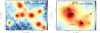 |
Fig. 2 NOEMA 1.3 mm continuum data for ISOSS22478 (left) and ISOSS23053 (right). The color scales show the 70 μm Herschel data and the contours present the 1.3 mm NOEMA continuum data. The contour levels are in steps of 3σ with the 1σ level of 57 μJy beam−1 for ISOSS22478 and 160 μJy beam−1 for ISOSS23053. Linear scale bars and the 1.3 mm beam size are shown. |
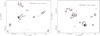 |
Fig. 3 NOEMA 1.3 mm continuum data for ISOSS22478 and ISOSS23053. The grey-scale and contours are now done in 5σ steps of 0.238 and 0.8 mJy beam−1 for ISOSS22478 and ISOSS23053, respectively. The red numbers label the identified cores. A linear scale bar and the 1.3 mm beam size are shown. |
Continuum parameters.
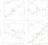 |
Fig. 4 Relations of core parameters. Top panels: peak column density and mean density plotted against the mass. Bottom panels: mean density and mass plotted against the equivalent radius. The red and blue colors always show the data for ISOSS22478 and ISOSS23053, respectively. The full pentagons show the results estimated assuming constant temperatures (T20K) whereas the crosses present the data assuming the temperatures derived from the H2CO line data ( |


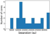 |
Fig. 5 Nearest-neighbor separation histogram from minimum spanning tree analysis for both regions combined. The spatial resolution limits are ~2700 and ~3500 au for ISOSS22478 and ISOSS23053, respectively. |
Linear minimum spanning tree analysis.
4.2 Kinematics and temperatures of the gas
We consider what the kinematics of the gas tell us about the formation processes within these two star-forming regions. To look at the dynamics in more detail, in the following we focus on the DCO+(3–2) emission that traces the gas properties at the given early evolutionary stage extremely well (e.g., Gerner et al. 2015). Figures 6 and 10 present an overview of the DCO+ data. The left panels show the integrated intensities and the middle and right panels present the 1st and 2nd moment maps (intensity-weighted peak velocities and velocity dispersions), respectively. These are always the merged datasets combining the NOEMA ACD configurations with the IRAM 30 m data (Sect. 3).
4.2.1 ISOSS22478
For ISOSS22478, the integrated emission clearly shows extended filamentary gas emission structures that connect the 1.3 mm continuum cores. The 1st moment map in the middle panel of Fig. 6 reveals a complex velocity structure with slightly different velocity components for the different sub-regions. We return to this point below. The velocity dispersion shown in the right panel shows on average low values largely around or even below 1 km s−1 (see also the cases of G29.96 and G35.20 for similarly narrow lines in deuterated ammonia, NH2D, Pillai et al. 2011). For comparison, Fig. 7 presents individual example spectra toward six cores. While the spectrum toward core #2 is better fitted with two components, some other spectra are still consistent with single-component fits. The full width half maximum (FWHM) Δv values are on average small and vary roughly between 0.6 and 1.5 km s−1 (thermal line width of DCO+ at 20 K ~ 0.17 km s−1).
A different way to look at the kinematics of the gas is to consider them as position-velocity slices along specific cuts within a region. Here, we concentrate on three slices marked in the middle panel of Fig. 6. Slice 1, connecting mainly cores #2 to #1 and #11, exhibits interesting multiple velocity components towards most of the core positions along the slice. Similarly, slice 3 also shows several velocity components at individual positions along the cut. In contrast to these two slices, the almost perpendicular cut, connecting mainly cores #6, #11, and #5 shows a different velocity gradient, with initially decreasing and then increasing velocities. Multiple velocity components at core positions have already been found in a few other regions (e.g., G035.39, G35.2, IRDC 18223, Orion, Henshaw et al. 2014; Sánchez-Monge et al. 2014; Beuther et al. 2015b; Hacar et al. 2017b). While such multiple velocity components can indicate the internal dynamics of the cores, for example thepresence of rotating structures (e.g., G35.2, Sánchez-Monge et al. 2014), these signatures have often been interpreted in the framework of fibers or interacting gas sheets. We return to this in Sect. 5.2.
Another important parameter is the temperature of the gas in the region. Figure 9 presents the temperature map we derived from the H2CO lines around 218 GHz (Table 1), which are a well-characterized thermometer of the interstellar gas (e.g., Mangum & Wootten 1993; Rodón et al. 2012; Gieser et al. 2019). To derive this temperature map, we used the eXtended CASA Line Analysis Software Suite (XCLASS, Möller et al. 20173) tool within the CASA software package (McMullin et al. 2007). In XCLASS the spectra are fitted pixel by pixel taking also the optical depth into account. The mean uncertainties for the temperatures are on the order of 30%. More details on the XCLASS fitting are given in Gieser et al. (2021). In addition to this, an in-depth analysis of the chemical and temperature structure of cores within the two regions will be presented in Gieser et al. (in prep.). As we can see in Fig. 9, the temperatures in ISOSS22478 are homogeneously very low, typically below 20 K, and only in the central part of the map do they rise above 20 K over some area. The temperature enhancement above 50 K in the small condensation in the south of the map (near the green contours in Fig. 9) is considered to be real because it is the only spot where also SiO(5–4) emission is detected. Hence, while we find at one localized position a temperature enhancement that seems to be associated with shocks, as suggested by the detection of SiO emission, we do not identify strong temperature differences along the main filamentary parts of the cloud. This is set into contrast to the SiO emission and temperature structure in ISOSS23053 below.
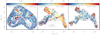 |
Fig. 6 NOEMA+30 m DCO+(3–2) data towards ISOSS22478. The three panels show in color scale the integrated intensity, the 1st and 2nd moment maps (intensity-weighted peak velocities and velocity dispersions), respectively. These maps were produced by clipping all data below an approximate 3σ threshold of 18 mJy beam−1. The contours show the 1.3 mm continuum emission in 3σ steps (1σ ~ 0.057 mJy beam−1) from 3 to 15σ. The beam is shown in the bottom-left of all panels, and a linear scale bar is shown in the middle panel. The red arrows in the middle panel show the three position velocity slices presented in Fig. 8. To reduce noise signatures at the edges of the mosaic, for the 1st and 2nd moment maps, we blanked the mosaic edges. The cores are labeled in the left panel. |
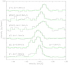 |
Fig. 7 DCO+(3–2) example spectra toward the labeled core positions in ISOSS22478 (Fig. 3). The spectra are shifted on the Y-axis for better presentation. The spectra of core #5 and core #6 are multiplied by 3 and 2 for clarity. The green lines show Gaussian fits, the FWHM linewidth Δv are presented for all spectra. For core #2, two components were fitted. |
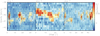 |
Fig. 8 Position-velocity diagrams in DCO+(3−2) for source ISOSS22478 along the cuts shown in Fig. 6. The contours are in 3σ steps of 18 mJy beam−1. The verticaldashed lines mark the positions of a few selected cores. |
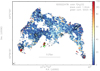 |
Fig. 9 Temperature map for ISOSS22478 derived from the H2CO line emission shown in color scale. The edges of the map are blanked because of the lower signal-to-noise ratio. The black contours present the 1.3 mm continuum starting at the 3σ level (1σ ~ 0.057 mJy beam−1) up to 15σ and then continue in 30σ steps. The green contours show SiO emission integrated from −44 to −38 km s−1 clipping all data below an approximate 4σ threshold of 30 mJy beam−1. The contour level is 0.2 Jy beam−1 km s−1. The beam isshown in the bottom-left, and a linear scale bar is shown as well. |
4.2.2 ISOSS23053
In comparison to ISOSS22478, the DCO+ gas emissionin ISOSS23053 looks very different (Fig. 10). Visually, a filamentary structure is less apparent. In comparison to ISOSS22478, where the DCO+ and mm continuum emission spatially agree relatively well, for ISOSS23053 many of the DCO+ peaks are offset from the main mm continuum peak positions. At the given spatial resolution, the corresponding continuum peak brightness temperatures are all below 1 K and the dust continuum emission is optically thin. Hence, dust optical depth effects cannot explain these offsets. More important in the context of the dynamical state of the region, the 1st moment map in Fig. 10 exhibits two very distinct velocity components that merge in the middle of the region on scales below 0.1 pc, right where we find most of the strong mm continuum cores. These two velocity components were already identified in previous NH3 data, and Bihr et al. (2015) suggested that they may be the signature of two converging gas streams that collide and trigger a new generation of star formation.
In that context, it is interesting to investigate the velocity dispersion. The 2nd moment map in Fig. 10 reveals that the velocity dispersion is largely low, at or below 1 km s−1. However, we see an increase in velocity dispersion above 1 km s−1 towards the main cores, and even higher values a bit to the north of the two main central cores (#2 & #3). Comparing these moment maps to a few selected spectra (Fig. 11), most of the spectra have rather narrow full width half maximum Δv values below 1.5 km s−1 with the exception of cores #1 and #2 that reveal Δv above 2 km s−1. The spectraalso show clearly the two velocity components, for instance, core #7 peaks around −54 km s−1 whereas the emission peak of core #8 is rather at −51 km s−1.
Regarding the two velocity components in ISOSS23053, Fig. 12 shows two position-velocity slices with the directions outlined in the middle panel of Fig. 10. Both slices clearly show the two velocity components that connect on very small spatial scales. While Bihr et al. (2015) report this velocity step as unresolved in their ~4″ NH3 observations and give a lower limit to the gradient of > 30 km s−1 pc−1, our higher spatial resolution allows us to better quantify this structure. For slices 1 and 2, we measure velocity gradients of ~48 km s−1 pc−1 and ~54 km s−1 pc−1, respectively.They can be even larger in the SiO emission discussed in the following.
In considering shocks by potential converging gas flows, we also investigate the SiO(5–4) emission presented in Fig. 13. Here, SiO is expected to be strongly enhanced by shocks because Si gets sputtered from the grains and quickly forms SiO in the gas phase (e.g., Schilke et al. 1997; Anderl et al. 2013). Interestingly, the SiO emission is comparably weak toward the main cores in the region, but it shows enhanced emission at several positions throughout the cloud. The strongest integrated SiO emission is identified between the main cores #2/#3 and #6. Additional significant SiO emission is found between the cores #1 and #5 as well as in some elongated structures toward the north of the region (e.g., one labeled as “stream” in Fig. 13). While the peak velocities in the 1st moment map show the same blue-red dichotomy as previously shown by the DCO+ data, the SiO linewidth increase visible in the 2nd moment map in Fig. 13 is very pronounced. We find increased velocity dispersion again between cores #2/#3 and #6 as well as between the cores #1 and #5 and the northern stream.
While SiO is often associated with shocks from outflows (e.g., Chandler & Richer 2001; Palau et al. 2006; Cabrit et al. 2012), shocks in a more general sense also from other drivers are sufficient (e.g., Anderl et al. 2013). For example, shocks during cloud formation may contribute to the SiO formation and emission as well (e.g., Jiménez-Serra et al. 2010, 2014). In the case of ISOSS23053, the stream-like features exhibit elongated structures that are most likely caused by outflows. The orientation of the stream-feature labeled in Fig. 13 is towards core #3, which may be the driver of that outflow structure. However, other strong SiO emission peaks, in particular those between the cores #1 and #5 as well as between cores #2/#3 and #6, do not necessarily need to be of protostellar outflow origin. Although core #1 is reported to drive an outflow (Birkmann et al. 2007), the strong SiO emission is rather centered between cores #1 and #5. All the SiO features between the cores #1/#5 and #2/#3/#6 are spatially closely linked to the velocity jump best visible in Fig. 10 or nearby core #6 in the SiO emission in Fig. 13. Conducting a position velocity cut approximately through core #6 (middle panel of Fig. 13), the corresponding position-velocity diagram is presented inFig. 14. The SiO emission along this cut covers a much broader velocity range than the DCO+ emission shown in Fig. 12. Furthermore, the two velocity components appear even more clearly separated in space.
While it cannot be entirely excluded that these velocity differences are of protostellar outflow origin, the clear spatial separation of the blue- and red-shifted emission without a clear driving source at its center make the outflow origin a less likely scenario. Quantifying the velocity jump in Fig. 14 from the two peak positions in the position velocity diagram at 3.0″/−57.1 km s−1 and 6.1″/−49.2 km s−1, we derive an estimate for the velocity gradient of ~122 km s−1 pc−1, more than twice the value found in the DCO+ emission. These velocity jumps are discussed in Sect. 5.2 in the context of potential converging gas flows.
The temperature structure in ISOSS23053 shows a different distribution compared to what we saw before for ISOSS22478. Figure 15 shows the gas temperature derived again from the H2CO emission lines in comparison with the 1.3 mm continuum (top panel) and the integrated SiO emission (bottom panel). While we still find significantly large areas with temperatures around 10 K (dark blue in Fig. 15), similarly large areas are already above 30 K (lighter blue). However, even more importantly, ISOSS23053 exhibits, in significant parts of the map, temperatures above 50 K and reaching even 100 K and above. If we compare these areas of enhanced temperatures with the dust continuum emission, that traces the dense cores, and with the SiO emission, that should trace the shocked gas, we clearly find that the high-temperature gas is preferentially associated with the shocks. This is not only the case for the areas between the main cores, but we also find this temperature increases toward the stream-like SiO structures that likely trace outflowing gas. However, we stress that the temperature enhancements as well as shock-tracing SiO emission are both found toward the region of the strong velocity jump in this regions. All these physical characteristics appear to be closely linked with what may happen in the case of converging gas flows (Sect. 5.2).
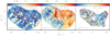 |
Fig. 10 NOEMA+30 m DCO+(3–2) data towards ISOSS23053. The three panels show in color scale the integrated intensity, the 1st and 2nd moment maps (intensity-weighted peak velocities and velocity dispersions), respectively. These maps were produced by clipping all data below an approximate 3σ threshold of 15 mJy beam−1. The contours show the 1.3 mm continuum emission in 3σ steps (1σ ~ 0.16 mJy beam−1) from 3 to 15σ. The beam isshown in the bottom-right of all panels, and a linear scale bar is shown in the middle panel. The arrows in the middle panel show the two position velocity slices presented in Fig. 12. To reduce noise signatures at the edges of the mosaic, for the 2nd moment map, we blanked the mosaic edges. The cores are labeled in the left panel. |
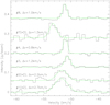 |
Fig. 11 DCO+(3–2) example spectra toward the labeled core positions in ISOSS23053 (Fig. 3). The spectra are shifted on the Y-axis for better presentation. The spectra of core #1, #2, and #7 and are multiplied by 2, 2, and 3 for clarity. The green lines show Gaussian fits and the FWHM linewidth Δv is presented for all spectral lines. |
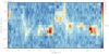 |
Fig. 12 Position-velocity diagrams in DCO+(3−2) for source ISOSS23053 along the cuts shown in Fig. 10. The contours are in 3σ steps of 18 mJy beam−1. The verticaldashed lines mark the positions of a few selected cores. |
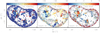 |
Fig. 13 NOEMA+30 m SiO(5–4) data towards ISOSS23053. The three panels show in color scale the integrated intensity, 1st and 2nd moment maps (intensity-weighted peak velocities and velocity dispersions), respectively. These maps were produced by clipping all data below an approximate 4σ threshold of 20 mJy beam−1. The contours show the 1.3 mm continuum emission in 3σ steps (1σ ~ 0.16 mJy beam−1). The beam is shown in the bottom-right of all panels, and a linear scale bar is shown in the middle panel. The cores are labeled in the left panel. The arrow in the middle panel marks the position-velocity cut presented in Fig. 14. |
5 Discussion
5.1 Fragmentation
Comparing the estimated masses and column densities to the corresponding values of the original CORE study of 20 high-mass star-formingregions in the more evolved evolutionary stages of high-mass protostellar objects (HMPOs), massive young stellar objects (mYSOs), and ultracompact HII regions (Beuther et al. 2018), we find that the masses are coveringa similar range. In contrast to that, the column densities of the original CORE sources are between ~1023 and ~1025 cm−2, about one order of magnitude larger than what we find here for the two younger regions. While this may be attributed to the younger evolutionary stage of the ISOSS sources presented here, we caution that the spatial resolution of the original CORE data was about a factor of 2 better (because of uniform weighting there and natural weighting here, see Sect. 3). Hence, with the higher spatial resolution, it was easier to resolve the highest column density peaks for the more evolved sources from the original CORE sample.
The mass-size relation shown in Fig. 4 is a bit puzzling because of the a priori uncertainty in the temperature estimates. While the T20K approach results in a mass-size relation with M ∝ r3.0 ± 0.2, which would correspond to constant mean volume densities for the sampled cores around 106 cm−3, the  approach results in a flatter mass-size relation M ∝ r2.0 ± 0.3. The latter agrees closely with the slope expected from Larson’s 3rd relation (e.g., Ballesteros-Paredes et al. 2020)and corresponds to constant mean column densities. In the literature, mass-size relations with various exponents can be found. While some studies report relations close to the classical r−2.0 (e.g., Heyer et al. 2009; Lombardi et al. 2010; Ballesteros-Paredes et al. 2019), steeper relations have been found as well. For example, Kainulainen et al. (2011) found a mass-size relation with exponent 2.7 when sampling only the highest column density parts of their studied molecular clouds (those regions where the column density probability density functions leave the lognormal shape and rather flatten out). It is interesting to note that also in the recent comparison between the extreme environments of the nuclear starburst of the extragalactic system NGC 253 and the central molecular zone of our Milky Way mass-size relations consistent with M ∝ r3 were found (Krieger et al. 2020).
Ballesteros-Paredes et al. (2012, 2019, 2020) discuss in detail the notion that mass-size relations with power-law indices from below 2 up to 3 have been reported in the literature (e.g., Mookerjea et al. 2004; Lada et al. 2008; Román-Zúñiga et al. 2010; Kainulainen et al. 2011; Könyves et al. 2015; Zhang & Li 2017; Veltchev et al. 2018). They reiterate that mass-size relations derived from constant column density thresholds (which is approximately the case for the 5σ intensity thresholds used here in the core finding algorithm), if the filling factor of the densest portions of the cores is small, should necessarily exhibit constant mean column densities, and thus, a M ∝ r2.0 relationship. However, if the small filling-factor hypothesis for the densest gas in the continuum data and core identification were not fulfilled (e.g., Fig. 3), the cores may exhibit sharp boundaries and the lower column density material would not contribute substantially to the mean column density. Such observational conditions would imply that the column density probability density functions (PDFs) do not fall as fast as necessary to produce a M ∝ r2.0 slope (Ballesteros-Paredes et al. 2012). Setting this picture into context with our observations, we cannot claim with certainty which temperature assumption is better for all cores and hence which mass-size relation, corresponding either to constant mean column density or to constant mean volume density. Possibly, some intermediate slope may represent the regions best. Hence, while our data are consistent with the classical 3rd Larson relation of constant mean column densities, some steeper slope, that results from not well sampled column density PDFs of the cores, cannot be excluded.
We can also set the derived masses and the projected nearest-neighbor separations into context within the classical Jeans analysis by estimating the Jeans masses and Jeans lengths for the typical parental gas clumps. Assuming mean volume densities of the original gas clump of ~ 105 cm−3 at temperatures of ~20 K (e.g., Hennemann et al. 2008), the corresponding Jeans length and Jeans mass (e.g., Stahler & Palla 2005) are ~17 500 au and ~0.9 M⊙, respectively.Both of these values are approximately in the regime of the majority of core masses and separations (Table 2 and Fig. 5). Estimating the mean nearest-neighbor separations, we get values of ~17 170 au and ~19 560 AU for ISOSS22478 and ISOSS23053, respectively. These values also agree roughly with the estimated Jeans length, similarly to what was found by Sanhueza et al. (2019).
To show this global trend in more detail for the individual cores, Fig. 16 presents the core masses versus the nearest neighbor separations, where the latter are used as proxies for the Jeans lengths. Corresponding relations for the Jeans analysis are shown there as well. While there is indeed scatter within the plot, the scatter is rather uniformly distributed around the typical Jeans relations. The scatter is slightly smaller for the masses derived with the  approach. Following Sanhueza et al. (2019), we can correct the nearest neighbor separations for average projection effects with an average correction factor of π∕2 ~ 1.57. This comparably small factor does not significantly affect the general correspondence of the Jeans relations and the data in Fig. 16.
This is again different to the original CORE sample of more evolved sources where the derived parameters scattered above the Jeans relations (Fig. 13 in Beuther et al. 2018). In that context, Beuther et al. (2018) considered what would happen if in the Jeans analysis, we replaced the thermal sound speed by the turbulent velocity dispersion. The expected relations would shift to the top-right in the mass-size relation, not improving the congruence between Jeans analysis and data. Furthermore, as visible in Figs. 7 and 11, the observed FWHM of individual spectral components are pretty low, typically around or even below 1 km s−1 (thermal line width of DCO+ at 20 K ~ 0.17 km s−1). Hence, turbulent contributions to the line width are less strong than would be expected in the turbulent core scenario of high-mass star formation (McKee & Tan 2003). Regarding filamentary fragmentation, in their ALMA study of very young high-mass star-forming regions Svoboda et al. (2019) estimated the cylindrical fragmentation scale to be roughly a factor of 3.5 of larger than the typical Jeans length. In that cylindrical framework, the Jeans regimes outlined in Fig. 16 (dashed and continuous lines) would shift by that factor to the right, almost outside the plot. Hence, cylindrical fragmentation seems not the most important process in our regions either.
These considerations further support the idea that thermal Jeans fragmentation can explain our data and that turbulence as well as cylindrical fragmentation are unlikely to play a significant role in the fragmentation of at least these two very young high-mass star-forming regions. Similar results have also been reported in, for example, Palau et al. (2014, 2015, 2018), Henshaw et al. (2017), Cyganowski et al. (2017), Klaassen et al. (2018) as well as in the recent ALMA studies of very young high-mass star-forming regions by Svoboda et al. (2019) and Sanhueza et al. (2019). However, there are also reports in the literature that support the notion that for some other sources, turbulent pressure may be more important (e.g., Wang et al. 2011, 2014; Zhang et al. 2015; Sadaghiani et al. 2020).
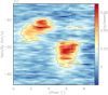 |
Fig. 14 Position-velocity diagrams in SiO(5−4) for source ISOSS23053 along the cut shown in Fig. 13 (middle panel). The contours are in 3σ steps of 22.5 mJy beam−1. The white dashed line marks the position of core #6. |
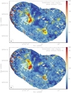 |
Fig. 15 Temperature map for ISOSS23053 derived from the H2CO line emission. Both panels show, in color scale, the derived temperatures with black contour levels of 50, 100, and 150 K. The high temperatures in particular at the eastern edge of the map are not real but are caused by the lower signal-to-noise ratio there. The yellow contours in the top and bottom panelspresent the 1.3 mm continuum and the integrated SiO(5–4) emission, respectively. The 1.3 mm continuum contours are in 3σ steps (1σ ~ 0.16 mJy beam−1). The SiO emission is integrated from −61 to −43 km s−1 clipping all data below an approximate 4σ threshold of 20 mJy beam−1. Contour levels are from 10 to 90% (step 10%) of the integrated peak emission of 1.58 Jy beam−1 km s−1. The beam isshown in the bottom-left of each panel, and a linear scale bar is shown as well. |
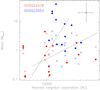 |
Fig. 16 Core masses against nearest-neighbor separations from the minimum spanning tree analysis. The full pentagons show the results estimated assuming constant temperatures (T20 K) whereas the crosses present the data assuming the temperatures derived from the H2CO line data ( |

5.2 Gas dynamics
While the original CORE program focused more on the fragmentation of the parental gas clumps and the inner massive disks (Beuther et al. 2018), the CORE-extension program here focuses on the dynamics of the gas clumps. It is interesting to see that the observations of the gas dynamics of the two target regions do differ in many ways (Sect. 4.2).
The intermediate-mass region ISOSS22478 exhibits a more filamentary structure with velocity gradients along and across the filaments as well as multiple velocity components at the locations of the cores. Similar kinematic signatures along filamentary low- and high-mass star-forming regions have been reported in, e.g., Fernández-López et al. (2014), Henshaw et al. (2014), Beuther et al. (2015b) or Hacar et al. (2017b). The temperature distribution of ISOSS22478 exhibits relatively uniform low temperatures between roughly 10 and 30 K. Furthermore, we do not find strong signatures of shocks, neither in SiO emission nor specific temperature enhancements.
In comparison, the more massive region ISOSS23053 does not show a particularly filamentary structure, however, a few of the cores are aligned along a narrow spatial strip where two different velocity components of two separate cloud structures overlap. Position-velocity slices across that strip clearly reveal two velocity components and a very steep gradient between the two components of roughly 50 km s−1 pc−1 measured in DCO+(3−2) and even ~122 km s−1 pc−1 measured in SiO(5−4). This velocity gradient is significantly larger than that reported by Hacar et al. (2017b) of 5–7 km s−1 pc−1 for the gravitational collapse of the OMC-1 molecular cloud. Furthermore, for ISOSS23053, the region of velocity overlap shows strong SiO emission as well as a large temperature increase from roughly 20 K in the environmental cloud up to 100 K and more in the velocity overlap region. The combination of a velocity jump, enhanced SiO emission as well as temperature increase are all indicative of shocks that may have been caused by converging or colliding gas flows.
These two regions may at first sight appear to represent two potentially different modes of cloud formation. However, the different signatures in the data could occur based on similar large-scale cloud collapse processes. Multiple velocity components along filamentary structures have regularly been observed in various star-forming regions of different masses (e.g., Hacar et al. 2013, 2018; Kirk et al. 2013; Fernández-López et al. 2014; Henshaw et al. 2014; Tackenberg et al. 2014; Beuther et al. 2015b; Dhabal et al. 2018), but there are also significant observational differences reported. For example, some regions of low and high mass reveal sub-filaments (or fibers) that may collide and form larger-scale filamentary structures during the formation process (e.g., Hacar et al. 2013, 2017a, 2018; Henshaw et al. 2014; Smith et al. 2014). Other observations have revealed velocity gradients across filaments (e.g., Palmeirim et al. 2013; Fernández-López et al. 2014; Beuther et al. 2015b; Shimajiri et al. 2019) that may be explained by gravity-induced accretion from a magnetized sheet-like molecular cloud (e.g., Chen & Ostriker 2015; Chen et al. 2020). However, we should keep in mind that in these clouds, often not just one signature exists but that several signatures occur within the same region. For example, studies of Serpens south as well as of IRDC 18223 reveal velocity gradients perpendicular to the clouds in some part of the filaments, but in other parts of the clouds thesestudies find clearly distinct multiple velocity components that may resemble more the sub-filament signatures (Fernández-López et al. 2014; Dhabal et al. 2018; Beuther et al. 2015b). Chen et al. (2020) point out that multiple velocity-components along a filament do not necessarily always have to be real structures but that the observational bias that different spectral lines trace different density regimes can also create artificial multiple velocity components in observations (see also Ballesteros-Paredes & Mac Low 2002; Zamora-Avilés et al. 2017). Different inclination angles and optical depth effects may also induce a similar bias in some data as well.
From a physical point of view, both scenarios, namely, colliding pre-existing filaments and gravity-induced accretion in sheet-like structures have a feature in common: both basically rely on the large-scale gravitational collapse of the molecular clouds. Low magnetization may result in more early fragmentation and then interacting pre-existing sub-filaments whereas higher magnetization should result in smoother structures and more coherent accretion onto filaments (see for example, Hennebelle & Inutsuka 2019, and references there in).
The distinct signature of a steep velocity gradient or even sharp velocity jump in ISOSS23053 can be interpreted as a signature of converging and colliding gas flows. For example, the cloud formation models with colliding flow conditions by Gómez & Vázquez-Semadeni (2014) produce similar velocity gradient structures, as seen in ISOSS23053. However, other simulations of cloud collapse, either hydrodynamic or magneto-hydrodynamic, can produce qualitatively similar velocity gradients as well (e.g., Smith et al. 2013; Chen et al. 2020). The outstanding aspect of the ISOSS23053 case is the steepness of the gradient with ≥50 km s−1 pc−1. While variations in inclination angles can induce differences in the slope of such a gradient, it is also possible that different physical properties, for instance, different magnetization or external compression may enhance the observed gradients. It appears that the smaller and smoother velocity gradients, as observed, for example, in the Serpens south, IRDC 18223, or the Orion integral shape filament (Fernández-López et al. 2014; Beuther et al. 2015b; Hacar et al. 2017b), can be explained mainly by gravitational collapse, whereas the sharp velocity jump observed here in ISOSS23053 may require an external cause that drives the converging gas flow. Gravitational collapse can then occur at the colliding flow interface.
Differentiating these variations requires additional observational as well as theoretical work. For example, it will be important to infer the magnetic field for a sample of clouds and investigate whether steep velocity gradients or multiple velocity components may correlate with the strength or orientation of the environmental magnetic fields. One obvious difference between the two regions is their Galactic latitude. While ISOSS23053 is close to the Galactic plane with a latitude of − 0.28 deg, ISOSS22478 is located at larger Galactic latitudes of + 4.26 deg. It is reasonable that closer to the Galactic plane, along with more star formation activity, there is also a more dynamic environment that can further amplify the potential dynamic gas structure and velocity gradients. On the simulation side, we would need to sample a broader range of magnetizations to infer whether stronger magnetic fields indeed favor smoother accretion onto filamentary structures, while lower magnetization may favor early formation of sub-filaments that could then collide during ongoing collapse.
What all of the above scenarios have in common is that they are based on a dynamical cloud collapse scenario that forms filamentary structures during the collapse motions. Environmental effects such as external shocks, converging gas flows or different magnetizations come into play, but they are all part of a dynamical collapse and fragmentation scenario.
6 Conclusions and summary
In the context of the NOEMA large program CORE, which studies, among other topics, the fragmentation processes during high-mass star formation, we studied two young regions of intermediate- to high-mass star formation, namely ISOSS22487and ISOSS23053. We used NOEMA and the IRAM 30 m telescope to produce high spatial resolution (~0.8″) mosaics to investigate their larger-scale fragmentation and cloud formation processes. In both regions, many fragments can be identified in the 1.3 mm continuum emission, and a diversity of spectral lines can be imaged over the entire field of view. We concentrate on the fragmentation based on the continuum emission, and on the kinematics of the clouds based on the DCO+, H2CO, and SiO emission. A forthcoming paper will present the entire spectral line data and a chemical analysis (Gieser et al., in prep.).
The 1.3 mm continuum data reveal 15 and 14 cores in ISOSS22478 and ISOSS23053, respectively. Most of them are associated with filamentary sub-structures in the cloud. Depending on the assumed temperatures of the cores, we estimate slightly different core masses. These differences then result in mass-size relations varying possibly between M ∝ r2 and M ∝ r3. Hence, while the data are consistent with the classical mass-size relation of r2 expected from the 3rd Larson relation for regions with constant mean column densities, a steeper relation cannot be ruled out. The latter could be explained because the cores in these maps have sharp boundaries and, thus, the lower iso-contours in the mm emission do not have much larger areas than higher iso-contours. Such steeper mass-size relation would correspond to similar mean densities for the cores. Furthermore, the correlation of the core masses with their nearest-neighbor separations is consistent with thermal Jeans fragmentation. In contrast to the original CORE sample of slightly more evolved sources, here, we barely find separations at our spatial resolution limit. Hence, our data resolve the large-scale fragmentation of the parental gas cloud well.
The kinematic analysis reveals very different observational signatures between the two regions. While ISOSS22478 is more filamentary in nature with several velocity components along the length of the filament, ISOSS23053 shows at the locations of the most massive cores a very steep velocity jump between two velocity components. The velocity gradient is roughly 50 km s−1 pc−1 measured in DCO+(3−2) and even ~122 km s−1 pc−1 measured in SiO(5−4). While these signatures appear disjointed at first sight, we argue that all these kinematic observations can be understood within the framework of dynamically collapsing clouds. Depending on the environmental properties, for example, external shocks causing converging gas flows or magnetized sheets that preferentially form filaments that accrete gas from the parental gas structure, different observational signatures of a global cloud collapse may be present. Further observational and theoretical investigations are needed to pin down in more detail how much the physical processes (e.g., magnetization, external compression) as well as the observational biases (e.g., tracers of different density, optical depth effects, inclination angles) contribute to the overall dynamical collapse of the clouds.
Acknowledgements
This work is based on observations carried out under project number L14AB with the IRAM NOEMA Interferometer and the IRAM 30 m telescope. IRAM is supported by INSU/CNRS (France), MPG (Germany) and IGN (Spain). We like to thank an anonymous referee for very useful comments. H.B. and S.S. acknowledge support from the European Research Council under the Horizon 2020 Framework Program via the ERC Consolidator Grant CSF-648505. H.B. also acknowledges support from the Deutsche Forschungsgemeinschaft in the Collaborative Research Center (SFB 881) “The Milky Way System” (subproject B1). A.P. acknowledges financial support from CONACyT and UNAM-PAPIIT IN113119 grant, México. D.S. acknowledges support by the Deutsche Forschungsgemeinschaft through SPP 1833: “Building a Habitable Earth” (SE 1962/6-1). R.K. acknowledges financial support via the Emmy Noether Research Group on Accretion Flows and Feedback in Realistic Models of Massive Star Formation funded by the German Research Foundation (DFG) under grant no. KU 2849/3-1 and KU 2849/3-2. JBP acknowledges financial support from CONACYT and UNAM-DGAPA-PAPIIT grant numbers 86372 and IN-111-219, respectively.
References
- Anderl, S., Guillet, V., Pineau des Forêts, G., & Flower, D. R. 2013, A&A, 556, A69 [NASA ADS] [CrossRef] [EDP Sciences] [Google Scholar]
- André, P., Di Francesco, J., Ward-Thompson, D., et al. 2014, in Protostars and Planets VI, eds. H. Beuther, R. Klessen, C. Dullemond, & T. Henning (Tucson: University of Arizona press), 27 [Google Scholar]
- Ballesteros-Paredes, J., & Mac Low, M.-M. 2002, ApJ, 570, 734 [NASA ADS] [CrossRef] [Google Scholar]
- Ballesteros-Paredes, J., D’Alessio, P., & Hartmann, L. 2012, MNRAS, 427, 2562 [NASA ADS] [CrossRef] [Google Scholar]
- Ballesteros-Paredes, J., Román-Zúñiga, C., Salomé, Q., Zamora-Avilés, M., & Jiménez-Donaire, M. J. 2019, MNRAS, 490, 2648 [Google Scholar]
- Ballesteros-Paredes, J., André, P., Hennebelle, P., et al. 2020, Space Sci. Rev., 216, 76 [CrossRef] [Google Scholar]
- Beltrán, M. T., & de Wit, W. J. 2016, A&ARv, 24, 6 [Google Scholar]
- Beuther, H., Churchwell, E. B., McKee, C. F., & Tan, J. C. 2007, in Protostars and Planets V, eds. B. Reipurth, D. Jewitt, & K. Keil (Tucson: University of Arizona Press), 165 [Google Scholar]
- Beuther, H., Linz, H., Tackenberg, J., et al. 2013, A&A, 553, A115 [NASA ADS] [CrossRef] [EDP Sciences] [Google Scholar]
- Beuther, H., Henning, T., Linz, H., et al. 2015a, A&A, 581, A119 [NASA ADS] [CrossRef] [EDP Sciences] [Google Scholar]
- Beuther, H., Ragan, S. E., Johnston, K., et al. 2015b, A&A, 584, A67 [NASA ADS] [CrossRef] [EDP Sciences] [Google Scholar]
- Beuther, H., Mottram, J. C., Ahmadi, A., et al. 2018, A&A, 617, A100 [NASA ADS] [CrossRef] [EDP Sciences] [Google Scholar]
- Bihr, S., Beuther, H., Linz, H., et al. 2015, A&A, 579, A51 [NASA ADS] [CrossRef] [EDP Sciences] [Google Scholar]
- Birkmann, S. M., Krause, O., Hennemann, M., et al. 2007, A&A, 474, 883 [NASA ADS] [CrossRef] [EDP Sciences] [Google Scholar]
- Bogun, S., Lemke, D., Klaas, U., et al. 1996, A&A, 315, L71 [NASA ADS] [Google Scholar]
- Bonnell, I. A., Larson, R. B., & Zinnecker, H. 2007, in Protostars and Planets V, eds. B. Reipurth, D. Jewitt, & K. Keil (Tucson: University of Arizona Press), 149 [Google Scholar]
- Cabrit, S., Codella, C., Gueth, F., & Gusdorf, A. 2012, A&A, 548, L2 [NASA ADS] [CrossRef] [EDP Sciences] [Google Scholar]
- Cesaroni, R., Galli, D., Lodato, G., Walmsley, C. M., & Zhang, Q. 2007, in Protostars and Planets V, ed. B. Reipurth, D. Jewitt, & K. Keil, 197 [Google Scholar]
- Chandler, C. J., & Richer, J. S. 2001, ApJ, 555, 139 [NASA ADS] [CrossRef] [Google Scholar]
- Chen, C.-Y., & Ostriker, E. C. 2015, ApJ, 810, 126 [NASA ADS] [CrossRef] [Google Scholar]
- Chen, C.-Y., Mundy, L. G., Ostriker, E. C., Storm, S., & Dhabal, A. 2020, MNRAS, 494, 3675 [CrossRef] [Google Scholar]
- Chira, R. A., Kainulainen, J., Ibáñez-Mejía, J. C., Henning, T., & Mac Low, M. M. 2018, A&A, 610, A62 [NASA ADS] [CrossRef] [EDP Sciences] [Google Scholar]
- Csengeri, T., Bontemps, S., Wyrowski, F., et al. 2017, A&A, 600, L10 [NASA ADS] [CrossRef] [EDP Sciences] [Google Scholar]
- Cyganowski, C. J., Brogan, C. L., Hunter, T. R., et al. 2014, ApJ, 796, L2 [NASA ADS] [CrossRef] [Google Scholar]
- Cyganowski, C. J., Brogan, C. L., Hunter, T. R., et al. 2017, MNRAS, 468, 3694 [NASA ADS] [CrossRef] [Google Scholar]
- Dhabal, A., Mundy, L. G., Rizzo, M. J., Storm, S., & Teuben, P. 2018, ApJ, 853, 169 [NASA ADS] [CrossRef] [Google Scholar]
- Di Francesco, J., Johnstone, D., Kirk, H., MacKenzie, T., & Ledwosinska, E. 2008, ApJS, 175, 277 [NASA ADS] [CrossRef] [Google Scholar]
- Draine, B. T. 2011, Physics of the Interstellar and Intergalactic Medium (Princeton: Princeton Series in Astrophysics) [Google Scholar]
- Feng, S., Beuther, H., Zhang, Q., et al. 2016, ApJ, 828, 100 [NASA ADS] [CrossRef] [Google Scholar]
- Fernández-López, M., Arce, H. G., Looney, L., et al. 2014, ApJ, 790, L19 [NASA ADS] [CrossRef] [Google Scholar]
- Gerner, T., Shirley, Y. L., Beuther, H., et al. 2015, A&A, 579, A80 [NASA ADS] [CrossRef] [EDP Sciences] [Google Scholar]
- Gieser, C., Semenov, D., Beuther, H., et al. 2019, A&A, 631, A142 [NASA ADS] [CrossRef] [EDP Sciences] [Google Scholar]
- Gieser, C., Beuther, H., Semenov, D., et al. 2021, A&A, 648, A66 [EDP Sciences] [Google Scholar]
- Gómez, G. C., & Vázquez-Semadeni, E. 2014, ApJ, 791, 124 [NASA ADS] [CrossRef] [Google Scholar]
- Hacar, A., Tafalla, M., Kauffmann, J., & Kovács, A. 2013, A&A, 554, A55 [NASA ADS] [CrossRef] [EDP Sciences] [Google Scholar]
- Hacar, A., Tafalla, M., & Alves, J. 2017a, A&A, 606, A123 [NASA ADS] [CrossRef] [EDP Sciences] [Google Scholar]
- Hacar, A., Alves, J., Tafalla, M., & Goicoechea, J. R. 2017b, A&A, 602, L2 [NASA ADS] [CrossRef] [EDP Sciences] [Google Scholar]
- Hacar, A., Tafalla, M., Forbrich, J., et al. 2018, A&A, 610, A77 [NASA ADS] [CrossRef] [EDP Sciences] [Google Scholar]
- Hennebelle, P. 2018, A&A, 611, A24 [NASA ADS] [CrossRef] [EDP Sciences] [Google Scholar]
- Hennebelle, P., & Inutsuka, S.-i. 2019, Front. Astron. Space Sci., 6, 5 [NASA ADS] [CrossRef] [Google Scholar]
- Hennemann, M., Birkmann, S. M., Krause, O., & Lemke, D. 2008, A&A, 485, 753 [NASA ADS] [CrossRef] [EDP Sciences] [Google Scholar]
- Henshaw, J. D., Caselli, P., Fontani, F., Jiménez-Serra, I., & Tan, J. C. 2014, MNRAS, 440, 2860 [NASA ADS] [CrossRef] [Google Scholar]
- Henshaw, J. D., Jiménez-Serra, I., Longmore, S. N., et al. 2017, MNRAS, 464, L31 [NASA ADS] [CrossRef] [Google Scholar]
- Heyer, M., Krawczyk, C., Duval, J., & Jackson, J. M. 2009, ApJ, 699, 1092 [NASA ADS] [CrossRef] [Google Scholar]
- Hildebrand, R. H. 1983, QJRAS, 24, 267 [NASA ADS] [Google Scholar]
- Jiménez-Serra, I., Caselli, P., Tan, J. C., et al. 2010, MNRAS, 406, 187 [NASA ADS] [CrossRef] [Google Scholar]
- Jiménez-Serra, I., Caselli, P., Fontani, F., et al. 2014, MNRAS, 439, 1996 [NASA ADS] [CrossRef] [Google Scholar]
- Kainulainen, J., Beuther, H., Banerjee, R., Federrath, C., & Henning, T. 2011, A&A, 530, A64 [NASA ADS] [CrossRef] [EDP Sciences] [Google Scholar]
- Kainulainen, J., Stutz, A. M., Stanke, T., et al. 2017, A&A, 600, A141 [NASA ADS] [CrossRef] [EDP Sciences] [Google Scholar]
- Kirk, H., Myers, P. C., Bourke, T. L., et al. 2013, ApJ, 766, 115 [NASA ADS] [CrossRef] [Google Scholar]
- Klaassen, P. D., Johnston, K. G., Urquhart, J. S., et al. 2018, A&A, 611, A99 [NASA ADS] [CrossRef] [EDP Sciences] [Google Scholar]
- Könyves, V., André, P., Men’shchikov, A., et al. 2015, A&A, 584, A91 [NASA ADS] [CrossRef] [EDP Sciences] [Google Scholar]
- Krause, O., Vavrek, R., Birkmann, S., et al. 2004, Balt. Astron., 13, 407 [Google Scholar]
- Krieger, N., Bolatto, A. D., Koch, E. W., et al. 2020, ApJ, 899, 158 [Google Scholar]
- Lada, C. J., Muench, A. A., Rathborne, J., Alves, J. F., & Lombardi, M. 2008, ApJ, 672, 410 [NASA ADS] [CrossRef] [Google Scholar]
- Larson, R. B. 1981, MNRAS, 194, 809 [Google Scholar]
- Li, S., Zhang, Q., Pillai, T., et al. 2019, ApJ, 886, 130 [NASA ADS] [CrossRef] [Google Scholar]
- Li, S., Sanhueza, P., Zhang, Q., et al. 2020a, ApJ, 903, 119 [Google Scholar]
- Li, S., Zhang, Q., Liu, H. B., et al. 2020b, ApJ, 896, 110 [Google Scholar]
- Lombardi, M., Alves, J., & Lada, C. J. 2010, A&A, 519, L7 [NASA ADS] [CrossRef] [EDP Sciences] [Google Scholar]
- Mangum, J. G., & Wootten, A. 1993, ApJS, 89, 123 [Google Scholar]
- McKee, C. F., & Tan, J. C. 2003, ApJ, 585, 850 [Google Scholar]
- McMullin, J. P., Waters, B., Schiebel, D., Young, W., & Golap, K. 2007, ASP Conf. Ser., 376, 127 [Google Scholar]
- Möller, T., Endres, C., & Schilke, P. 2017, A&A, 59, A7 [Google Scholar]
- Mookerjea, B., Kramer, C., Nielbock, M., & Nyman, L. Å. 2004, A&A, 426, 119 [NASA ADS] [CrossRef] [EDP Sciences] [Google Scholar]
- Motte, F., Bontemps, S., Schilke, P., et al. 2007, A&A, 476, 1243 [NASA ADS] [CrossRef] [EDP Sciences] [Google Scholar]
- Nony, T., Louvet, F., Motte, F., et al. 2018, A&A, 618, L5 [NASA ADS] [CrossRef] [EDP Sciences] [Google Scholar]
- Ossenkopf, V., & Henning, T. 1994, A&A, 291, 943 [NASA ADS] [Google Scholar]
- Padoan, P., Pan, L., Juvela, M., Haugbølle, T., & Nordlund, Å. 2020, ApJ, 900, 82 [Google Scholar]
- Palau, A., Ho, P. T. P., Zhang, Q., et al. 2006, ApJ, 636, L137 [NASA ADS] [CrossRef] [Google Scholar]
- Palau, A., Estalella, R., Girart, J. M., et al. 2014, ApJ, 785, 42 [NASA ADS] [CrossRef] [Google Scholar]
- Palau, A., Ballesteros-Paredes, J., Vázquez-Semadeni, E., et al. 2015, MNRAS, 453, 3785 [NASA ADS] [CrossRef] [Google Scholar]
- Palau, A., Zapata, L. A., Román-Zúñiga, C. G., et al. 2018, ApJ, 855, 24 [NASA ADS] [CrossRef] [Google Scholar]
- Palmeirim, P., André, P., Kirk, J., et al. 2013, A&A, 550, A38 [NASA ADS] [CrossRef] [EDP Sciences] [Google Scholar]
- Peretto, N., Fuller, G. A., André, P., et al. 2014, A&A, 561, A83 [NASA ADS] [CrossRef] [EDP Sciences] [Google Scholar]
- Peters, T., Klessen, R. S., Mac Low, M.-M., & Banerjee, R. 2010, ApJ, 725, 134 [Google Scholar]
- Pillai, T., Kauffmann, J., Wyrowski, F., et al. 2011, A&A, 530, A118 [NASA ADS] [CrossRef] [EDP Sciences] [Google Scholar]
- Ragan, S., Henning, T., Krause, O., et al. 2012, A&A, 547, A49 [NASA ADS] [CrossRef] [EDP Sciences] [Google Scholar]
- Ragan, S. E., Henning, T., Beuther, H., Linz, H., & Zahorecz, S. 2015, A&A, 573, A119 [NASA ADS] [CrossRef] [EDP Sciences] [Google Scholar]
- Rodón, J. A., Beuther, H., & Schilke, P. 2012, A&A, 545, A51 [NASA ADS] [CrossRef] [EDP Sciences] [Google Scholar]
- Román-Zúñiga, C. G., Alves, J. F., Lada, C. J., & Lombardi, M. 2010, ApJ, 725, 2232 [NASA ADS] [CrossRef] [Google Scholar]
- Román-Zúñiga, C. G., Alfaro, E., Palau, A., et al. 2019, MNRAS, 489, 4429 [CrossRef] [Google Scholar]
- Sadaghiani, M., Sánchez-Monge, Á., Schilke, P., et al. 2020, A&A, 635, A2 [CrossRef] [EDP Sciences] [Google Scholar]
- Sánchez-Monge, Á., Beltrán, M. T., Cesaroni, R., et al. 2014, A&A, 569, A11 [NASA ADS] [CrossRef] [EDP Sciences] [Google Scholar]
- Sanhueza, P., Contreras, Y., Wu, B., et al. 2019, ApJ, 886, 102 [NASA ADS] [CrossRef] [Google Scholar]
- Schilke, P., Walmsley, C. M., Pineau des Forets, G., & Flower, D. R. 1997, A&A, 321, 293 [NASA ADS] [Google Scholar]
- Schneider, N., Csengeri, T., Bontemps, S., et al. 2010, A&A, 520, A49 [NASA ADS] [CrossRef] [EDP Sciences] [Google Scholar]
- Schuller, F., Menten, K. M., Contreras, Y., et al. 2009, A&A, 504, 415 [NASA ADS] [CrossRef] [EDP Sciences] [Google Scholar]
- Shimajiri, Y., André, P., Palmeirim, P., et al. 2019, A&A, 623, A16 [NASA ADS] [CrossRef] [EDP Sciences] [Google Scholar]
- Smith, R. J., Clark, P. C., & Bonnell, I. A. 2009, MNRAS, 396, 830 [NASA ADS] [CrossRef] [Google Scholar]
- Smith, R. J., Shetty, R., Beuther, H., Klessen, R. S., & Bonnell, I. A. 2013, ApJ, 771, 24 [NASA ADS] [CrossRef] [Google Scholar]
- Smith, R. J., Glover, S. C. O., & Klessen, R. S. 2014, MNRAS, 445, 2900 [Google Scholar]
- Sokolov, V., Wang, K., Pineda, J. E., et al. 2018, A&A, 611, L3 [CrossRef] [EDP Sciences] [Google Scholar]
- Stahler, S. W., & Palla, F. 2005, The Formation of Stars (Hoboken: Wiley-VCH) [Google Scholar]
- Svoboda, B. E., Shirley, Y. L., Traficante, A., et al. 2019, ApJ, 886, 36 [Google Scholar]
- Tackenberg, J., Beuther, H., Henning, T., et al. 2014, A&A, 565, A101 [NASA ADS] [CrossRef] [EDP Sciences] [Google Scholar]
- Tan, J. C., Beltrán, M. T., Caselli, P., et al. 2014, Protostars and Planets VI (Tucson: University of Arizona Press), 149 [Google Scholar]
- Tan, J. C., Kong, S., Zhang, Y., et al. 2016, ApJ, 821, L3 [NASA ADS] [CrossRef] [Google Scholar]
- VanderPlas, J., Connolly, A. J., Ivezic, Z., & Gray, A. 2012, in Proceedings of Conference on Intelligent Data Understanding (CIDU), 47 [Google Scholar]
- Veltchev, T. V., Ossenkopf-Okada, V., Stanchev, O., et al. 2018, MNRAS, 475, 2215 [Google Scholar]
- Wang, K., Zhang, Q., Wu, Y., & Zhang, H. 2011, ApJ, 735, 64 [NASA ADS] [CrossRef] [Google Scholar]
- Wang, K., Zhang, Q., Testi, L., et al. 2014, MNRAS, 439, 3275 [NASA ADS] [CrossRef] [Google Scholar]
- Williams, J. P., de Geus, E. J., & Blitz, L. 1994, ApJ, 428, 693 [NASA ADS] [CrossRef] [Google Scholar]
- Zamora-Avilés, M., Ballesteros-Paredes, J., & Hartmann, L. W. 2017, MNRAS, 472, 647 [NASA ADS] [CrossRef] [Google Scholar]
- Zhang, C.-P., & Li, G.-X. 2017, MNRAS, 469, 2286 [NASA ADS] [CrossRef] [Google Scholar]
- Zhang, Q., Wang, K., Lu, X., & Jiménez-Serra, I. 2015, ApJ, 804, 141 [NASA ADS] [CrossRef] [Google Scholar]
- Zinnecker, H., & Yorke, H. W. 2007, ARA&A, 45, 481 [NASA ADS] [CrossRef] [Google Scholar]
See also http://www.mpia.de/core
All Tables
All Figures
|
Fig. 1 Overview of the ISOSS22478+6357 (left) and ISOSS23053 (right) regions. The color scales and contours show the 70 and 450 μm emission from Herschel and SCUBA, respectively (Ragan et al. 2012; Di Francesco et al. 2008). The contour levels are from 18 to 98% of the peak emission of 1.88 and 14.88 Jy beam−1 for the two regions, respectively. Linear scale bars are shown and the red circles outline the NOEMA mosaics with a primary beam FWHM of 22″. |
| In the text | |
|
Fig. 2 NOEMA 1.3 mm continuum data for ISOSS22478 (left) and ISOSS23053 (right). The color scales show the 70 μm Herschel data and the contours present the 1.3 mm NOEMA continuum data. The contour levels are in steps of 3σ with the 1σ level of 57 μJy beam−1 for ISOSS22478 and 160 μJy beam−1 for ISOSS23053. Linear scale bars and the 1.3 mm beam size are shown. |
| In the text | |
|
Fig. 3 NOEMA 1.3 mm continuum data for ISOSS22478 and ISOSS23053. The grey-scale and contours are now done in 5σ steps of 0.238 and 0.8 mJy beam−1 for ISOSS22478 and ISOSS23053, respectively. The red numbers label the identified cores. A linear scale bar and the 1.3 mm beam size are shown. |
| In the text | |
|
Fig. 4 Relations of core parameters. Top panels: peak column density and mean density plotted against the mass. Bottom panels: mean density and mass plotted against the equivalent radius. The red and blue colors always show the data for ISOSS22478 and ISOSS23053, respectively. The full pentagons show the results estimated assuming constant temperatures (T20K) whereas the crosses present the data assuming the temperatures derived from the H2CO line data ( |
| In the text | |
|
Fig. 5 Nearest-neighbor separation histogram from minimum spanning tree analysis for both regions combined. The spatial resolution limits are ~2700 and ~3500 au for ISOSS22478 and ISOSS23053, respectively. |
| In the text | |
|
Fig. 6 NOEMA+30 m DCO+(3–2) data towards ISOSS22478. The three panels show in color scale the integrated intensity, the 1st and 2nd moment maps (intensity-weighted peak velocities and velocity dispersions), respectively. These maps were produced by clipping all data below an approximate 3σ threshold of 18 mJy beam−1. The contours show the 1.3 mm continuum emission in 3σ steps (1σ ~ 0.057 mJy beam−1) from 3 to 15σ. The beam is shown in the bottom-left of all panels, and a linear scale bar is shown in the middle panel. The red arrows in the middle panel show the three position velocity slices presented in Fig. 8. To reduce noise signatures at the edges of the mosaic, for the 1st and 2nd moment maps, we blanked the mosaic edges. The cores are labeled in the left panel. |
| In the text | |
|
Fig. 7 DCO+(3–2) example spectra toward the labeled core positions in ISOSS22478 (Fig. 3). The spectra are shifted on the Y-axis for better presentation. The spectra of core #5 and core #6 are multiplied by 3 and 2 for clarity. The green lines show Gaussian fits, the FWHM linewidth Δv are presented for all spectra. For core #2, two components were fitted. |
| In the text | |
|
Fig. 8 Position-velocity diagrams in DCO+(3−2) for source ISOSS22478 along the cuts shown in Fig. 6. The contours are in 3σ steps of 18 mJy beam−1. The verticaldashed lines mark the positions of a few selected cores. |
| In the text | |
|
Fig. 9 Temperature map for ISOSS22478 derived from the H2CO line emission shown in color scale. The edges of the map are blanked because of the lower signal-to-noise ratio. The black contours present the 1.3 mm continuum starting at the 3σ level (1σ ~ 0.057 mJy beam−1) up to 15σ and then continue in 30σ steps. The green contours show SiO emission integrated from −44 to −38 km s−1 clipping all data below an approximate 4σ threshold of 30 mJy beam−1. The contour level is 0.2 Jy beam−1 km s−1. The beam isshown in the bottom-left, and a linear scale bar is shown as well. |
| In the text | |
|
Fig. 10 NOEMA+30 m DCO+(3–2) data towards ISOSS23053. The three panels show in color scale the integrated intensity, the 1st and 2nd moment maps (intensity-weighted peak velocities and velocity dispersions), respectively. These maps were produced by clipping all data below an approximate 3σ threshold of 15 mJy beam−1. The contours show the 1.3 mm continuum emission in 3σ steps (1σ ~ 0.16 mJy beam−1) from 3 to 15σ. The beam isshown in the bottom-right of all panels, and a linear scale bar is shown in the middle panel. The arrows in the middle panel show the two position velocity slices presented in Fig. 12. To reduce noise signatures at the edges of the mosaic, for the 2nd moment map, we blanked the mosaic edges. The cores are labeled in the left panel. |
| In the text | |
|
Fig. 11 DCO+(3–2) example spectra toward the labeled core positions in ISOSS23053 (Fig. 3). The spectra are shifted on the Y-axis for better presentation. The spectra of core #1, #2, and #7 and are multiplied by 2, 2, and 3 for clarity. The green lines show Gaussian fits and the FWHM linewidth Δv is presented for all spectral lines. |
| In the text | |
|
Fig. 12 Position-velocity diagrams in DCO+(3−2) for source ISOSS23053 along the cuts shown in Fig. 10. The contours are in 3σ steps of 18 mJy beam−1. The verticaldashed lines mark the positions of a few selected cores. |
| In the text | |
|
Fig. 13 NOEMA+30 m SiO(5–4) data towards ISOSS23053. The three panels show in color scale the integrated intensity, 1st and 2nd moment maps (intensity-weighted peak velocities and velocity dispersions), respectively. These maps were produced by clipping all data below an approximate 4σ threshold of 20 mJy beam−1. The contours show the 1.3 mm continuum emission in 3σ steps (1σ ~ 0.16 mJy beam−1). The beam is shown in the bottom-right of all panels, and a linear scale bar is shown in the middle panel. The cores are labeled in the left panel. The arrow in the middle panel marks the position-velocity cut presented in Fig. 14. |
| In the text | |
|
Fig. 14 Position-velocity diagrams in SiO(5−4) for source ISOSS23053 along the cut shown in Fig. 13 (middle panel). The contours are in 3σ steps of 22.5 mJy beam−1. The white dashed line marks the position of core #6. |
| In the text | |
|
Fig. 15 Temperature map for ISOSS23053 derived from the H2CO line emission. Both panels show, in color scale, the derived temperatures with black contour levels of 50, 100, and 150 K. The high temperatures in particular at the eastern edge of the map are not real but are caused by the lower signal-to-noise ratio there. The yellow contours in the top and bottom panelspresent the 1.3 mm continuum and the integrated SiO(5–4) emission, respectively. The 1.3 mm continuum contours are in 3σ steps (1σ ~ 0.16 mJy beam−1). The SiO emission is integrated from −61 to −43 km s−1 clipping all data below an approximate 4σ threshold of 20 mJy beam−1. Contour levels are from 10 to 90% (step 10%) of the integrated peak emission of 1.58 Jy beam−1 km s−1. The beam isshown in the bottom-left of each panel, and a linear scale bar is shown as well. |
| In the text | |
|
Fig. 16 Core masses against nearest-neighbor separations from the minimum spanning tree analysis. The full pentagons show the results estimated assuming constant temperatures (T20 K) whereas the crosses present the data assuming the temperatures derived from the H2CO line data ( |
| In the text | |
Current usage metrics show cumulative count of Article Views (full-text article views including HTML views, PDF and ePub downloads, according to the available data) and Abstracts Views on Vision4Press platform.
Data correspond to usage on the plateform after 2015. The current usage metrics is available 48-96 hours after online publication and is updated daily on week days.
Initial download of the metrics may take a while.