| Issue |
A&A
Volume 649, May 2021
|
|
|---|---|---|
| Article Number | A137 | |
| Number of page(s) | 33 | |
| Section | Extragalactic astronomy | |
| DOI | https://doi.org/10.1051/0004-6361/202038605 | |
| Published online | 28 May 2021 | |
The physical properties of local (U)LIRGs: A comparison with nearby early- and late-type galaxies
1
National Observatory of Athens, Institute for Astronomy, Astrophysics, Space Applications and Remote Sensing, Ioannou Metaxa and Vasileos Pavlou, 15236 Athens, Greece
e-mail: This email address is being protected from spambots. You need JavaScript enabled to view it.
2
Section of Astrophysics, Astronomy & Mechanics, Department of Physics, Aristotle University of Thessaloniki, 54124 Thessaloniki, Greece
3
Sterrenkundig Observatorium, Universiteit Gent, Krijgslaan 281 S9, 9000 Gent, Belgium
4
INAF – Osservatorio Astrofisico di Arcetri, Largo E. Fermi 5, 50125 Florence, Italy
5
Department of Astrophysics, Astronomy & Mechanics, Faculty of Physics, University of Athens, Panepistimiopolis, 15784 Zografos Athens, Greece
6
Instituto de Fisica de Cantabria (CSIC-Universidad de Cantabria), Avenida de los Castros, 39005 Santander, Spain
Received:
7
June
2020
Accepted:
5
February
2021
Abstract
Aims. In order to pinpoint the place of the (ultra-) luminous infrared galaxies ((U)LIRGs) in the local Universe, we examine the properties of a sample of 67 such nearby systems and compare them with those of 268 early- and 542 late-type, well studied, galaxies from the DustPedia database.
Methods. We made use of multi-wavelength photometric data (from the ultra-violet to the sub-millimetre), culled from the literature, and the CIGALE spectral energy distribution fitting code to extract the physical parameters of each system. The median spectral energy distributions as well as the values of the derived parameters were compared to those of the local early- and late-type galaxies. In addition to that, (U)LIRGs were divided into seven classes, according to the merging stage of each system, and variations in the derived parameters were investigated.
Results. (U)LIRGs occupy the ‘high-end’ on the dust mass, stellar mass, and star-formation rate (SFR) plane in the local Universe with median values of 5.2 × 10⁷ M⊙, 6.3 × 10¹⁰ M⊙, and 52 M⊙ yr−1, respectively. The median value of the dust temperature in (U)LIRGs is 32 K, which is higher compared to both the early-type (28 K) and the late-type (22 K) galaxies. The dust emission in PDR regions in (U)LIRGs is 11.7% of the total dust luminosity, which is significantly higher than early-type (1.6%) and late-type (5.2%) galaxies. Small differences in the derived parameters are seen for the seven merging classes of our sample of (U)LIRGs with the most evident one being on the SFR, where in systems in late merging stages (‘M3’ and ‘M4’) the median SFR reaches up to 99 M⊙ yr−1 compared to 26 M⊙ yr−1 for the isolated ones. In contrast to the local early- and late-type galaxies where the old stars are the dominant source of the stellar emission, the young stars in (U)LIRGs contribute with 64% of their luminosity to the total stellar luminosity. The fraction of the stellar luminosity absorbed by the dust is extremely high in (U)LIRGs (78%) compared to 7% and 25% in early- and late-type galaxies, respectively. The fraction of the stellar luminosity used to heat up the dust grains is very high in (U)LIRGs, for both stellar components (92% and 56% for the young and the old stellar populations, respectively) while 74% of the dust emission comes from the young stars.
Key words: galaxies: evolution / galaxies: ISM / galaxies: interactions / dust, extinction / galaxies: star formation / galaxies: stellar content
© ESO 2021
1. Introduction
A multi-wavelength approach is needed for a comprehensive study of galaxies. Each region of the electromagnetic spectrum provides unique information about the different building blocks of galaxies (stars, dust, and gas) and their physical properties. These building blocks constituting the baryonic matter in galaxies are not in isolation, but, instead, they are constantly interacting with each other, modifying the stellar content and the interstellar medium (ISM). This evolutionary process is imprinted on the galaxy’s spectral energy distribution (SED). Studying the SEDs of galaxies is, thus, a key procedure towards understanding galaxy formation and evolution.
One property, often related to the degree of the current star-formation is the infrared (IR) luminosity (LIR = L8−1000 μm), which, in most cases, is dominated by the emission of dust grains heated by the interstellar radiation field (ISRF). Early-type galaxies (elliptical and lenticular galaxies) exhibit very low to moderate IR luminosities (LIR < 109 L⊙), while the star-forming spiral galaxies are brighter in the IR (109 < LIR/L⊙ < 1011; Lonsdale et al. 2006). Imaging studies of (Ultra-) Luminous Infrared Galaxies ((U)LIRGs; LIR > 1011 L⊙) in the local Universe indicate a more violent kind of formation of these systems with the majority of them exhibiting signs of galaxy interactions (Sanders & Mirabel 1996; Duc et al. 1997). Armus et al. (1987) concluded that more than ∼70% of such systems show signs of interactions originating from merging events between their parent galaxies. Later studies of IR-luminous galaxies (Melnick & Mirabel 1990; Hutchings & Neff 1991; Clements et al. 1996) indicate even larger fractions (∼90%) of the sources in their samples being mergers, while other studies concluded that fractions of such sources are lower than 70% (Lawrence et al. 1989; Zou et al. 1991; Leech et al. 1994). In all cases, however, it becomes clear that galaxy merging is a key process that is responsible for the high IR luminosity and drives the high level of star-formation activity observed in these systems, making them a unique class of objects in the local Universe.
The mid-infrared (MIR) part of the SED is a very complex regime where different components of the galaxy contribute to the emission. The SED in these wavelengths can be a mixture of light originating from old stellar populations, emission of dust grains (mainly heated by newly formed stars), as well as radiation emitted by an active galactic nucleus (AGN). In (U)LIRGs, the MIR spectra can probe the conditions in their star-forming regions, to which they owe their high luminosities. Although galaxy interactions can trigger and enhance nuclear activity in local (U)LIRGs, star-formation processes dominate the MIR emission in the majority of these systems (Genzel et al. 1998; Petric et al. 2011; Stierwalt et al. 2013). The UV and optical radiation emitted by the newly formed stars in dusty molecular clouds is absorbed and then re-emitted by dust in IR wavelengths. Dust emission is seen either through emission features (e.g., polycyclic aromatic hydrocarbons; PAHs) or continuum emission originating from the photo-dissociation regions (PDRs), as well as dust diffusely distributed throughout the galaxy.
One way to decompose the SED of a galaxy and extract useful information on the different components contributing to their emission is by using SED-fitting codes. Such codes usually make use of templates for the emission of different components combined in such a way so that energy is conserved. Assuming two different stellar populations (old and young stars) and a certain variation in the star-formation activity through cosmic time (i.e. the star-formation history; SFH), several characteristic properties of the galaxies can be determined by fitting their observed SEDs. Such properties are stellar and dust masses, luminosities, and the star-formation rate (SFR). In addition to the stellar and dust components, an AGN component can be considered when needed. The decomposition of the galactic SEDs has lead to versatile studies of the properties of galaxies (Giovannoli et al. 2011; Małek et al. 2014; Pappalardo et al. 2016; Małek et al. 2014; Pappalardo et al. 2016; Vika et al. 2017), and more specifically, studies about the attenuation processes (Boquien et al. 2013; Salim et al. 2018) or the contribution of the different stellar populations in the heating of dust and the dependence on the morphological type (Bianchi et al. 2018; Nersesian et al. 2019).
In this paper we model the SEDs of 67 IR-luminous local galaxies in order to derive their physical properties and to investigate how these properties compare with other types of galaxies in the local Universe. We explore how several physical properties, such as the SFR, the stellar mass and the dust mass, dust temperature, and PDR luminosity vary with galaxy type. By dividing (U)LIRGs into different classes, according to the interaction of their parent galaxies, we investigate the evolution of all the aforementioned parameters with a merging stage. Finally, we examine the relative contributions of the different stellar populations to the bolometric luminosity of galaxies and their role in the dust heating. By comparing our results with a recent study on passive and star-forming galaxies (Nersesian et al. 2019), we determine the role of each stellar population in the dust heating and its variations for the different types of galaxies in the local Universe.
This paper is structured as follows. The sample analysed in this work is presented in Sect. 2 followed by a description of the SED fitting method in Sect. 3. The results of our analysis as well as a comparison of the properties of the (U)LIRGs in our sample with those of ‘normal’ galaxies in the local Universe are explored in Sect. 4. The evolution of the physical properties of (U)LIRGs with a merging stage is investigated in Sect. 5, while the different stellar populations and their role in the heating of the dust grains is discussed in Sect. 6. Our findings are summarised in Sect. 7. Finally, a mock analysis, performed by CIGALE, is presented in Appendix A, the best-fit SED models are shown in Appendix B, a comparison with other studies is performed in Appendix C, while the cumulative distributions of various physical parameters are presented in Appendix D.
2. The sample
Our main sample consists of 67 local (U)LIRGs (see Table 1) drawn from the Great Observatories All-sky LIRG Survey (GOALS; Armus et al. 2009). All sources have sufficient wavelength coverage with an average of eight observations in the UV/optical/NIR (<3 μm) part of the spectrum and 16 in the MIR/FIR/submm (>3 μm) part of the spectrum (see Table 1, but also the corresponding SEDs in Fig. B.1). This allows us to conduct a full SED fitting study and derive valuable information on the intrinsic properties of the sources.
Properties of the (U)LIRGs in our sample.
All galaxies have been observed by the Herschel Space Observatory (HSO; Pilbratt et al. 2010) with the corresponding photometry published in Chu et al. (2017). In this study, total system fluxes (if systems of galaxies consist of more than one galaxy) and component fluxes (where possible) were computed for all six Herschel bands (PACS (70, 100, and 160 μm) and SPIRE (250, 350, and 500 μm)). The photometric apertures were carefully chosen, first by visual inspection, and, subsequently, by plotting the curve of growth and checking that all of the flux was included.
Apart from the Herschel photometry, the rest of the multi-wavelength data were compiled from two literature resources, the photometry presented in U et al. (2012; for 64 galaxies) and the photometry presented in Clark et al. (2018; for three galaxies; F06107+7822, F10257-4339, and F23133-4251, in the DustPedia1 database). All the details for the data assembly and treatment are discussed in the relevant papers. In summary, the space-based observations include ultraviolet data from GALEX (Morrissey et al. 2007, FUV; λeff = 0.15 μm, and NUV; λeff = 0.23 μm), MIR data from Spitzer/IRAC (Werner et al. 2004, 3.6, 4.6, 5.4, and 8 μm), and FIR data from Spitzer/MIPS (Werner et al. 2004, 24, 70, and 160 μm). IRAS data at 12, 25, 60, and 100 μm as published in the Revised Bright Galaxy Sample (RBGS; Sanders et al. 2003) have also been incorporated into our analysis. Concerning the ground-based data, the main source in optical wavebands are observations taken with the University of Hawaii (UH) 2.2 m Telescope on Mauna Kea with the remaining optical data compiled from the literature and the NASA/IPAC Extragalactic Database (NED; see U et al. 2012, and references therein). Near-infrared J, H, and Ks were extracted from the Two Micron All Sky Survey (2MASS; Skrutskie et al. 2006). Sub-millimetre data at 850 μm and 450 μm, obtained using the Submillimetre Common User Bolometer Array (SCUBA) at the James Clerk Maxwell Telescope, were taken from Dunne et al. (2000) and Dunne & Eales (2001). In both of these studies, a careful aperture-matched photometry was performed on the data sets, securing a consistent photometry among the different photometric bands. In the case of U et al. (2012), masked photometry has been extracted from the images taken at effective wavelengths, 0.15 μm < λeff< 8 μm, and at MIPS 24 μm band with the masks defined based on isophotes in the median- and boxcar-smoothed I-band images at the surface brightness limit of 24.5 mag arcsec−2 so that the global flux from tidal debris as well as individual components within these merger systems are encapsulated. For the remaining wavelengths, masks would not improve the precision of the total flux due to a lack in resolution, so circular or elliptical apertures were used. In Clark et al. (2018), the photometry and uncertainty estimation in all bands is done within a master elliptical aperture, which is found after combining the elliptical apertures fitted in each band, separately, in such a way so that the different beam sizes are taken into account.
Out of these 67 systems, the vast majority (56) are LIRGs (LIR > 1011 L⊙), whereas 11 are ULIRGs (LIR > 1012 L⊙). Their redshifts range from 0.003 to 0.083 with a mean value of 0.029, while ∼80% of the galaxies are in the redshift range between 0.01 and 0.04. Their IR luminosities (based on IRAS photometry by Sanders et al. 2003) as well as their redshift distribution are presented in Fig. 1 (see also Table 1).
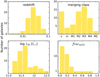 |
Fig. 1. Distributions of the basic properties of our galaxy sample. The redshift distribution is plotted in the top-left panel and the number of sources per merging class is in the top-right panel. In the bottom-left panel, the IR luminosity distribution, based on IRAS observations (Sanders et al. 2003) is shown, while the bolometric AGN fractions calculated in Díaz-Santos et al. (2017) are plotted in the bottom-right panel. |
Since merging is a key process in the regulation of the properties of these systems, we also wanted to analyse the properties of our sample considering their different merging stages. For the classification of their stage, we have used the categorisation adopted in Larson et al. (2016). In that paper, optical imaging data from the GOALS HST sample (PID: 10592, PI: Evans; Kim et al. 2013) as well as optical I-band images obtained with the UH 2.2 m telescope on Mauna Kea by Ishida (2004) were used to visually classify the galaxies. Several criteria were imposed to conduct the classification, all being discussed in detail in Larson et al. (2016). For the sake of completeness, here, we briefly repeat the broad characteristics of the seven different merging classes, as originally introduced by Larson et al. (2016), along with their abbreviation:
– s: single galaxies: galaxies that show no current sign of an interaction or merger event.
– m: minor mergers: interacting pairs with estimated mass ratios > 4:1.
– M1: major merger-stage 1: pairs that appear to be on their initial approach and have no prominent tidal features; with low relative velocity and galaxy separation, ΔV < 250 km s−1, nsep < 75 kpc.
– M2: major merger-stage 2: interacting galaxy pairs with obvious tidal bridges and tails (Toomre & Toomre 1972) or other disturbances consistent with having already undergone a first close passage.
– M3: major merger-stage 3: merging galaxies with multiple nuclei. These systems have distinct nuclei in disturbed, overlapping disks, along with visible tidal tails.
– M4: major merger-stage 4: galaxies with apparent single nuclei and obvious tidal tails. The galaxy nuclei have nsep ≤ 2 kpc.
– M5: major merger-stage 5: galaxies which appear to be evolved merger remnants. These galaxies have diffuse envelopes which may exhibit shells or other fine structures (Schweizer & Seitzer 1992) and a single, possibly off-centre nucleus. These merger remnants no longer have bright tidal tails. Examples of galaxies in the different classes are illustrated in Fig. 1 of Larson et al. (2016).
Two of the galaxies in our sample (namely, F10173+0828 and F01076-1707) were classified as ambiguous (amb) in Larson et al. (2016). F10173+0828 appears to have a single nucleus with faint tidal tails which would have resulted in an ‘M4’ classification; however, a second smaller disturbed galaxy (SDSS CGB24551.1) can be a possible companion, but with no reported redshift. F01076-1707 was previously classified as a non-interacting galaxy by Stierwalt et al. (2013). The galaxy consists of a diffuse disk and a possible disconnected diffuse tail (∼37 kpc to the west), though, it is unclear if this diffuse structure is the remnant of a tidal tail. In order to ease the analysis, we have chosen to keep their most obvious classification in place (i.e. ‘M4’ for F10173+0828 and ‘s’ for F01076-1707), although we caution the reader that these two galaxies may be missclassified. The three galaxies drawn from the DustPedia database have been classified by us by visually inspecting their optical images. F06107+7822 shows signs of an evolved merger remnant with a single nucleus and was thus classified as ‘M5’. F10257-4339 shows a system of merging galaxies with two distinct nuclei in disturbed overlapping disks and with obvious tidal tails, thus it is classified as ‘M3’. Finally, F23133-4251 shows no current signs of interaction or merger events and is thus classified as ‘s’.
The classification of the systems in our sample is presented in Fig. 1 (see also Table 1). In total, our sample consists of 14 ‘s’, four ‘m’, six ‘M1’, 14 ‘M2’, 17 ‘M3’, ten ‘M4’, and two ‘M5’ systems. We caution the reader that a few merging classes are under-represented (e.g., ‘m’ and ‘M5’), so their statistical significance in the following analysis may be questionable. In the subsequent SED analysis, systems with multiple components are treated as one system (a similar approach already presented in U et al. 2012). Even though this concept is correct (if multiple systems are bound dynamically, they should be treated as one), it possesses some limitations on the validity of the SED fitting, especially for multiple systems with the parent galaxies being separated by large distances from each other (e.g., ‘M1’ systems) where the galaxies (with different properties) are forced to be treated as one entity. In such systems, we assume that the SED modelling that was performed produced an average description of each multiple system.
Since nearby (U)LIRGs constitute a separate class of galactic systems in the local Universe, which show high IR luminosities and enhanced SFR by definition, we need to have a reference sample of ‘normal’ galaxies (in the sense of being less active in forming stars; either passive (ETGs) or low level star-forming galaxies (LTGs)) for comparison purposes. The most complete, up to date, sample of local galaxies is that of DustPedia (Davies et al. 2017; Clark et al. 2018). This sample includes 875 galaxies (with distances of less than 40 Mpc) all having Herschel detections, with D25 > 1′ (D25 being the major axis isophote at which optical surface brightness falls beneath 25 mag arcsec−2). Additionally, the DustPedia sample mostly includes isolated galaxies that have a detected stellar component; WISE observations at 3.4 μm are the deepest all-sky data sensitive to the stellar component of galaxies, and hence they provide the most consistent way of implementing this stellar detection requirement. For full sample details, see Davies et al. (2017) and Clark et al. (2018). Furthermore, the DustPedia sample contains galaxies of various morphologies parametrised by the Hubble stage (T; Makarov et al. 2014) ranging from T = −5 (pure elliptical galaxies) to T = 10 (irregular galaxies). Throughout our analysis we consider galaxies with T < 0.5 as ETGs and galaxies with T ≥ 0.5 as LTGs. Out of these 875 galaxies, 814 were successfully modelled using the CIGALE (Code Investigating GALaxy Emission) SED fitting tool (Boquien et al. 2019), with only three of them (NGC2146, NGC3256, and NGC7552) overlapping with our current sample since they are LIRGs. The products of this modelling are available in the DustPedia database with a full description given in Nersesian et al. (2019).
3. SED modelling
In order to exploit the information hidden in the SEDs of the galaxies, we make use of CIGALE (see Boquien et al. 2019, and references therein). CIGALE models the SED of each galaxy by selecting a suitable set of parameters through a Bayesian approach that best represents the observed SED. A basic principle of the code is the conservation of the energy between the amount absorbed by the dust and that re-emitted by the dust grains in infrared and sub-millimetre wavelengths (Roehlly et al. 2014). In the current study, we use the version 2020.0 of CIGALE. Beyond many improvements and optimisations related to the diminution of the computational time and the estimation of the physical properties, the most important new feature is related to the AGN model used. In addition to the active nucleus model formulated by Fritz et al. (2006), the SKIRTOR module (Stalevski et al. 2012, 2016) has been added. Following recent theoretical and observational studies (Nikutta et al. 2009; Ichikawa et al. 2012; Stalevski et al. 2012; Tanimoto et al. 2019), SKIRTOR assumes a two-phase dusty clumpy torus, where most of the dust has a high density and is clumpy, while the rest is smoothly distributed. SKIRTOR is based on the 3D radiative transfer code SKIRT (Baes et al. 2011; Camps & Baes 2015). In addition, this version of CIGALE includes not only torus obscuration, but also obscuration by dust settled along polar directions, allowing for a more precise treatment of both type-1 and type-2 AGN cases (Bongiorno et al. 2012; Elvis et al. 2012; Stalevski et al. 2017, 2019; Lyu & Rieke 2018).
The stellar radiation field is built based on the Bruzual & Charlot (2003) population synthesis model and a Salpeter (1955) initial mass function (IMF). After the fitting procedure, the stellar emission can be decomposed into two distinct populations, an old and a young population, depending on the SFH of each galaxy. To account for the starlight attenuation by dust, a modified Calzetti et al. (2000) starburst attenuation law is applied (Noll et al. 2009) to the intrinsic spectra of the different stellar populations. For the dust emission properties, we adopted the THEMIS model (Jones et al. 2017). In addition, we used a flexible SFH that gets an analytical expression of a delayed SFH allowing for an instantaneous burst (or quenching) of the star-formation activity (see, Ciesla et al. 2015 and Nersesian et al. 2019). Since all of the galaxies in our sample are actively forming stars, we only used the bursting mode of the delayed SFH (over the last 10–100 Myr) with six cases of instantaneous bursts (at various levels) and one case with no burst. The nuclear activity of local (U)LIRGs has already been investigated by others (e.g., Nardini et al. 2010; Ricci et al. 2017; U et al. 2019). In a series of two papers (C-GOALS I Iwasawa et al. 2011 and C-GOALS II Torres-Albà et al. 2018), a total of 107 (U)LIRGs from the GOALS sample were observed with the Chandra X-ray Observatory, revealing AGN signatures for 31 ± 5% and 38 ± 7% of the two sub-samples respectively. Careful treatment of the AGN component is, therefore, necessary for the purposes of the current study. To account for a realistic description of the AGN emission, we made use of the SKIRTOR module, which also includes polar-dust extinction. The parameter space of this module follows the parametrisation presented in Yang et al. (2020), except for the values of polar dust colour excess, E(B-V), where only two values were used (0, 0.8). This was indicated by Mountrichas et al. (2021), who find that CIGALE is not very sensitive in this parameter.
Concerning the input parameters used in CIGALE, except from those defining the AGN module, we adopted a similar parameter space as the one used in Nersesian et al. (2019) and modified it accordingly so that it is able to successfully model the SEDs of the systems in the current sample. By performing several test runs with CIGALE, we were able to minimise the number of values that control the SFH and the dust modules, in favour of the SKIRTOR module, taking into account the computational demands imposed by the total number of parameters. These test runs indicated values of the parameters that were not used by CIGALE and thus were excluded from the parameter space, resulting in the final input parameter grid listed in Table 2. The attenuation law considered here (Calzetti et al. 2000) was also tested against that of the widely adopted Charlot & Fall (2000) attenuation law. Both the shape of the SEDs and the output parameters between the two cases were found to be comparable and within the uncertainties.
Grid of input parameters used in CIGALE for the best-fit model computation.
In order to assess whether or not physical properties can actually be estimated in a reliable way, we performed a mock analysis by using the relevant feature built in CIGALE. The results of the mock analysis are presented and discussed in Appendix A. The modelled SEDs of all the systems in our sample are presented in Fig. B.1. To further evaluate the CIGALE-derived properties, we perform a comparison with other studies in Appendix C.
4. The physical properties and SEDs of local (U)LIRGs
The values and associated uncertainties of the physical properties (Mstar, Mdust, Tdust, SFR, fracAGN), as derived by CIGALE, for each source in our sample, along with the reduced χ2 of the fit, are listed in Table 3. (U)LIRGs are systems of enhanced IR luminosity and, as such, are expected to show up as the dustiest and most actively star-forming galaxies in the local Universe (as already shown in previous studies, see, e.g., da Cunha et al. 2010a and U et al. 2012). The mean dust mass of the galaxies in our sample is ⟨Mdust⟩=7.2 × 10⁷ M⊙, ranging from Mdust = 9.5 × 10⁶ M⊙ for F13126+2453 to Mdust = 3.8 × 10⁸ M⊙ for F15327+2340. Concerning the current SFR, we computed a mean value of ⟨SFR⟩=81 M⊙ yr−1 ranging from 2.7 M⊙ yr−1 for F13197-1627 to 410.8 M⊙ yr−1 for F14348-1447. As a comparison, the dustier and more actively star-forming ‘normal’ galaxies in the local Universe (those of morphological classes Sb-Sc) show an average dust mass of 2 × 10⁷ M⊙ and an average SFR of 2.4 M⊙ yr−1 (Nersesian et al. 2019). (U)LIRGs are also amongst the most massive galaxies in the local Universe with a mean value of their stellar mass of ⟨Mstar⟩ = 8.6 × 10¹⁰ M⊙, ranging from Mstar = 4.3 × 10⁹ M⊙ for F12224-0624 to Mstar = 3.2 × 10¹¹M⊙ for F14547+2449. Local elliptical galaxies, being the most massive amongst the ‘normal’ galaxies, show a mean stellar mass of 8.3 × 10¹⁰M⊙ (Nersesian et al. 2019).
CIGALE-derived physical properties of the (U)LIRGs in our sample.
4.1. The SEDs of (U)LIRGs
The SEDs of galaxies have been proven to be valuable assets for characterising their content in stars and dust, as well as their current star-formation activity. Even by visual inspection of the SEDs, one can spot the differences between different populations and this is what we do next by comparing, in a statistically significant and systematic way, the SEDs of local ETGs, LTGs, and (U)LIRGs.
In our analysis, we have modelled the SEDs of the 67 local (U)LIRGs in our sample, using CIGALE, and compare them with those of 268 ETGs and 542 LTGs, already modelled in Nersesian et al. (2019). This comparison is shown in Fig. 2 with the median SEDs of ETGs, LTGs, and (U)LIRGs in the top-left, top-right, and bottom-left panels, respectively. In the bottom-right panel, we present the median SEDs of ETGs, LTGs, and (U)LIRGs (red, blue, and yellow curves, respectively) so that a direct comparison can be made. For each of the three classes, both the attenuated and the unattenuated SEDs are also shown (thick solid lines and thin dotted lines, respectively, in the UV-optical part of the SED). The most obvious change among them is the differences in the IR and UV wavelength regimes of the SEDs, and, more specifically, at the peak of the dust emission (around 100 μm) and the peak of the stellar emission (around 1 μm).
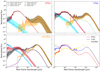 |
Fig. 2. Template SEDs of the DustPedia ETGs (top-left panel), LTGs (top-right panel), and the local (U)LIRGs (bottom-left panel), as modelled by CIGALE. The black curves indicate the median SEDs, while the blue and red curves denote the median unattenuated SEDs of the young and old stellar populations, respectively. The median distribution of the diffuse dust is shown by the orange curve and the emission from the PDRs is shown by the green curve. The purple curve, in the bottom-left panel, indicates the median AGN distribution. The shaded areas cover the range between the 16th and 84th percentiles to the median values. For clarity reasons, since the PDR and the AGN components may vary substantially, we chose not to present the percentile widths of the curves. The median SEDs of the three different types of local galaxies are plotted in the bottom-right panel. The red curve represents the median, observed, SED of ETGs, the blue curve represents the one of LTGs, while the yellow curve corresponds to the median SED of (U)LIRGs. The thin, dotted curves show the unattenuated total stellar emission for the different classes. The reader is also referred to the corresponding median SEDs in Bianchi et al. (2018) and Nersesian et al. (2019). |
What is clearly visible is that the dust emission shows a large variation with the peak being higher by 1.17 dex for LTGs (compared to ETGs), and higher by 0.56 dex for (U)LIRGs (compared to LTGs). This already dictates the differences in dust content among the three populations with ETGs being the most devoid and (U)LIRGs the abundant ones. The slight shift in the peak (in the wavelength axis) seen in the dust SED inclines towards a variation in dust temperature with LTGs being the cooler ones and (U)LIRGs the warmest ones. The actual wavelength where the peak of the FIR emission happens is at 96, 116, and 70 μm for ETGs, LTGs, and (U)LIRGs, respectively. The dust emission, as treated by CIGALE, consists of two components, one accounting for the diffuse dust and one accounting for the PDRs, which is mostly associated with the star-forming regions (Hollenbach & Tielens 1999). From Fig. 2 (green curves), we see that the significance of the dust in the PDR regions increases from ETGs (having negligible, practically non-existent emission) to LTGs (with a significant, but still, less dominant contribution compared to the diffuse dust) to (U)LIRGs (where the PDR emission is comparable to the diffuse dust emission in the 5–30 μm wavelength range, with a clear effect on the shape of the SED in this region). The shape of the SED in this wavelength range can also be affected by the presence of an AGN (purple curve), though there are only a few galaxies (∼12%) in our sample with strong or moderate AGN activity as revealed by CIGALE, with fracAGN > 0.2. Such examples are F13197-1627 and F23254+0830, where a large part of their SEDs (even at FIR wavelengths) are dominated by the AGN component (see their SEDs in Fig. B.1). It is worth noting though that in the MIR wavelength range, where both the emission from the PDRs and the AGN contribute, a degeneracy between the two components may be present, especially in cases of strong AGNs.
The observed, stellar SED, on the other hand, shows the opposite trend, with the peak (measured at 1 μm) being the highest for ETGs, slightly lower (by 0.23 dex) for LTGs, and much lower (by 1.95 dex) for (U)LIRGs (compared to ETGs). This happens, of course, when the dust effects are considered, and so stellar light is re-processed under different levels of attenuation, depending on the dust content in different galaxy populations. This picture changes substantially when the unattenuated stellar light is considered (see the thin dotted lines in the SEDs in the bottom-right panel in Fig. 2). The most obvious change is seen in the FUV (0.15 μm) where the (U)LIRGs show the highest emission, followed by the LTGs (lower by 0.37 dex) and with the ETGs showing about two orders of magnitude less emission (1.95 dex) compared to the (U)LIRGs. The effects of dust attenuation are better seen in the UV wavelengths, with the ETGs showing only a very small change between attenuated and unattenuated curves (a difference of 0.28 dex at 0.15 μm; a combination of both small amounts of dust and a small fraction of young stars). These effects are more prominent for LTGs where a decent amount of dust is present (a change by 0.78 dex), while it is severe for (U)LIRGs (a change of 2.44 dex between attenuated and unattenuated curves) where large amounts of dust dim the stellar light. What is also interesting is that, in (U)LIRGs, the attenuation by the dust starts to become significant short-wards of ∼2 μm and so both stellar populations (old and young) are significantly affected (better seen in the bottom-left panel of Fig. 2). For LTGs, the dust effects on the stellar populations are seen short-wards of ∼1 μm, but they significantly affect only the young stars (see the top-right panel of Fig. 2), while for ETGs, the effect is negligible, making its presence obvious in wavelengths short-wards of ∼0.2 μm with a small change in the emission of the young stars (top-left panel of Fig. 2).
4.2. Local (U)LIRGs: A comparison with early- and late-type galaxies
The existence of a very tight correlation between the SFR and the stellar mass for star-forming galaxies (often referred to as the ‘main-sequence’) is well established, not only for local galaxies (see, e.g., Elbaz et al. 2007; Whitaker et al. 2012; Davies et al. 2019, and references therein) but also for galaxies at high redshifts (see, e.g., Brinchmann et al. 2004; Elbaz et al. 2007; Wuyts et al. 2011b; Magdis et al. 2012; Chang et al. 2015; Pearson et al. 2018, and references therein). Local galaxies of various morphologies (ranging from pure ellipticals to irregulars) occupy different loci in the SFR/Mstar plane with the most prominent ones being the two distinct sequences, one for the star-forming galaxies (with high SFRs) and one for the more relaxed systems (with low SFRs), with a third population occupying the space in between (see, e.g., Davies et al. 2019, and references therein). This is presented in Fig. 3 (top panel) with the blue circles being the LTGs (galaxies with T ≥ 0.5) and the red circles being the ETGs (galaxies with T < 0.5). A linear regression to the LTGs (cyan dotted line) gives
![Mathematical equation: $$ \begin{aligned} \mathrm{log} (\textit{SFR}[{{M}_{\odot }}\, \mathrm{yr} ^{-1}]) = 0.75\,\mathrm{log} (M_\mathrm{star} [{M}_{\odot }]) - 7.78, \end{aligned} $$](/articles/aa/full_html/2021/05/aa38605-20/aa38605-20-eq1.gif)
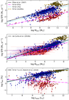 |
Fig. 3. Correlations of SFR with stellar mass and dust mass (upper and middle panels respectively), and between fabs and Lbolo (bottom panel; see the text for the definition of the parameters). The DustPedia ETGs and LTGs are shown with red and blue circles, respectively, while yellow stars are the local (U)LIRGs in our sample. All values are plotted along with their corresponding uncertainties. In all plots, magenta dash-dotted, cyan dotted, and yellow dashed lines are the linear fits to the ETGs, LTGs, and (U)LIRGs, respectively. The black solid lines correspond to the best fits found in Elbaz et al. (2007) to the 0.015 ≤ z ≤ 0.1 SDSS star-forming galaxies (top panel), to the best fit found in da Cunha et al. (2010b) for a sample of low redshift galaxies (middle panel), and to the best fit found in Bianchi et al. (2018) for the DustPedia galaxies with T ≥ 2.5 (bottom panel). |
with a Spearman’s correlation coefficient (Spearman 1904) of ρ = 0.69, indicating a moderate positive correlation, while the same relation for ETGs (magenta dash-dotted line) is
![Mathematical equation: $$ \begin{aligned} \mathrm{log} (\textit{SFR}[{M}_{\odot }\,\mathrm{yr} ^{-1}]) = 0.61\ \mathrm{log} (M_\mathrm{star} [{M}_{\odot }]) - 7.93, \end{aligned} $$](/articles/aa/full_html/2021/05/aa38605-20/aa38605-20-eq2.gif)
with ρ = 0.44, indicating a moderate positive correlation, as well. For comparison, we overplotted the relation for SDSS star-forming galaxies at 0.015 ≤ z ≤ 0.1 (black solid line) found in Elbaz et al. (2007). Overall we find a good agreement between our fit to the star-forming galaxies and that of Elbaz et al. (2007), with the slopes differing slightly (0.77 in Elbaz et al. 2007 compared to 0.75 in the current study) and with an offset of 0.4 dex at Mstar = 5 × 10⁹ M⊙, which is to be expected, though, since the galaxies in Elbaz et al. (2007) extend to larger redshifts. The evolution with redshift is well studied by several works (e.g., Whitaker et al. 2014; Johnston et al. 2015; Schreiber et al. 2015).
Completing the picture in the local Universe, we include the nearest (U)LIRGs (yellow stars). What is immediately evident is that these systems are amongst the most massive (with stellar masses above ∼1010 M⊙) and the most actively star-forming ones, with a clear threshold in the SFR above ∼10 M⊙ yr−1, covering the high end of the main-sequence. A linear regression to this population gives
![Mathematical equation: $$ \begin{aligned} \mathrm{log} (\textit{SFR}[{M}_{\odot }\, \mathrm{yr} ^{-1}]) = 0.02\ \mathrm{log} (M_{\mathrm{star} }[{M}_{\odot }]) + 1.52 \end{aligned} $$](/articles/aa/full_html/2021/05/aa38605-20/aa38605-20-eq3.gif)
(yellow dashed line). For this population of local galaxies, we see an almost flat relation between Mstar and the SFR (slope of 0.02), indicating no evident correlation. This is also supported by the value of the Spearman’s correlation coefficient being very close to zero (ρ = −0.1), indicating a very weak correlation. Such behaviour is to be expected since the parameter space for this population of galaxies is somehow limited with their values bounded by their high-end Mstar and SFR extremes. Similar results are also presented in previous studies analysing samples of local luminous galaxies, for example in da Cunha et al. (2010a) and Kilerci Eser et al. (2014).
A similar behaviour is seen, even more clearly, by comparing the SFR with the dust mass (middle panel in Fig. 3). Here, the different symbols are the same as in the top panel. It is obvious that (U)LIRGs are a separate population of local galaxies with both the SFR (as mentioned above) and the dust mass occupying the high ends of these quantities (with Mdust being above ∼107 M⊙). A linear regression to the DustPedia LTGs in the SFR-Mdust plane gives
![Mathematical equation: $$ \begin{aligned} \mathrm{log} (\textit{SFR}[{M}_{\odot }\, \mathrm{yr} ^{-1}]) = 0.81\ \mathrm{log} (M_\mathrm{dust} [{M}_{\odot }]) - 5.8, \end{aligned} $$](/articles/aa/full_html/2021/05/aa38605-20/aa38605-20-eq4.gif)
(cyan dotted line) with a Spearman’s correlation coefficient of ρ = 0.8, indicating a strong correlation, while this relation for the ETGs becomes
![Mathematical equation: $$ \begin{aligned} \mathrm{log} (\textit{SFR}[{M}_{\odot }\, \mathrm{yr} ^{-1}]) = 0.8\ \mathrm{log} (M_\mathrm{dust} [{M}_{\odot }]) - 6.27, \end{aligned} $$](/articles/aa/full_html/2021/05/aa38605-20/aa38605-20-eq5.gif)
(magenta dash-dotted line) with ρ = 0.67 indicating a moderate correlation. Our findings are in fair agreement with the relation found in da Cunha et al. (2010b) studying a sample of star-forming galaxies from the SDSS at z ≤ 0.22 (see the black solid line in the middle panel of Fig. 3) with the slope of the linear regression in their sample (0.9) being slightly higher than the one we find (0.81 for the LTGs).
As expected, local (U)LIRGs occupy a different regime of the SFR-Mdust space, which is also indicated by the following best-fit relation,
![Mathematical equation: $$ \begin{aligned} \mathrm{log} (\textit{SFR}[{M}_{\odot }\, \mathrm{yr} ^{-1}]) = 0.39\ \mathrm{log} (M_\mathrm{dust} [{M}_{\odot }]) - 1.29 \end{aligned} $$](/articles/aa/full_html/2021/05/aa38605-20/aa38605-20-eq6.gif)
(yellow dashed line) with the slope (0.39) indicating a much flatter distribution with respect to the LTGs and ETGs (slopes of 0.81 and 0.8 respectively). This is also supported by the Spearman’s correlation coefficient being very low (ρ = 0.22), indicating a weak monotonic increase in the SFR with Mdust.
Although local (U)LIRGs exhibit increased SFR with respect to the normal star-forming galaxies (by more than an order of a magnitude; see the transition from blue circles to yellow stars in the top and middle panels of Fig. 3), this is not the case for the ratio of dust luminosity to the bolometric luminosity (fabs = Ldust/Lbolo). This quantity (discussed in detail in Bianchi et al. 2018) indicates the significance of the dust in galaxies and the effectiveness of the dust grains in absorbing the stellar radiation (a combination of the total amount of dust, the geometry, and the strength of the ISRF), which, in turn, is re-emitted at FIR/submm wavelengths. This is shown in the bottom panel of Fig. 3 with fabs plotted against the bolometric luminosity (Lbolo). Here, the different symbols are the same as in the top panel. A linear regression to the data gives
![Mathematical equation: $$ \begin{aligned} \mathrm{log} (f_\mathrm{abs} [\%]) = 0.32\ \mathrm{log} (L_\mathrm{bolo} [{L}_{\odot }]) - 1.94, \end{aligned} $$](/articles/aa/full_html/2021/05/aa38605-20/aa38605-20-eq7.gif)
for LTGs (cyan dotted line) and,
![Mathematical equation: $$ \begin{aligned} \mathrm{log} (f_\mathrm{abs} [\%]) = -0.08\ \mathrm{log} (L_\mathrm{bolo} [{L}_{\odot }]) + 1.12, \end{aligned} $$](/articles/aa/full_html/2021/05/aa38605-20/aa38605-20-eq8.gif)
for ETGs (magenta dash-dotted line) with Spearman’s correlation coefficients of 0.62 and −0.07, respectively, indicating a moderate correlation of fabs increasing with Lbolo for LTGs, but a very weak decrease for ETGs. The black solid line is the best-fit linear relation for LTGs with T ≥ 2.5, as originally presented by Bianchi et al. (2018), which is almost identical to what we find (including galaxies with 0.5 ≤ T < 2.5). Even though the local (U)LIRGs occupy the high end of the bolometric luminosity, their fabs values show a smooth transition from the respective values of the star-forming galaxies (see the differences among the different styles of data points in the bottom panel of Fig. 3), reaching a plateau for large values of Lbolo. This plateau is expected since the fabs cannot exceed 100% and is also indicated by the slope of the best-fit to the data (yellow dashed line),
![Mathematical equation: $$ \begin{aligned} \mathrm{log} (f_\mathrm{abs} [\%]) = 0.12\ \mathrm{log} (L_\mathrm{bolo} [{L}_{\odot }]) + 0.51, \end{aligned} $$](/articles/aa/full_html/2021/05/aa38605-20/aa38605-20-eq9.gif)
but also from the Spearman’s coefficient of the data (0.46) indicating a moderate correlation of fabs increasing with Lbolo. A more detailed comparison of the values of fabs between the different populations of local galaxies will follow (Sect. 6).
In Fig. 4 we have plotted several physical properties of the three samples of galaxies (ETGs, LTGs, and (U)LIRGs) so that we can visualise and quantify the differences. In all cases, red, blue, and yellow symbols correspond to ETGs, LTGs, and (U)LIRGs, respectively. The right-hand side plots in each panel show the histograms of the relevant quantity for the three galaxy populations. In addition, in Appendix D, we have plotted the relevant cumulative distributions of the parameters for each galaxy population (Fig. D.1) and report the p-values (Table D.1) of the Kolmogorov-Smirnov (KS hereafter) tests Smirnov (1948).
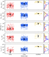 |
Fig. 4. Physical properties, as derived by CIGALE, for the different galaxy types. From top to bottom, Mdust, Mstar, sSFR, Tdust, and LPDR are plotted as a function of galaxy type. Each red and blue dot corresponds to an individual ETG and LTG galaxy, while yellow dots correspond to (U)LIRGs, respectively. Black diamonds stand for the median values per galaxy type, while the associated 16th and 84th percentile ranges are indicated with error bars. Side plots of the distributions of each galaxy type for all the physical properties are also presented, following the same colouring as for the dots. In the bottom panel (LPDR), the median value of ETGs is dragged down to lower values because CIGALE predicts no PDR contribution for some sources (see the text for more details). |
In the top panel, we show the variation in dust mass. As already stated earlier in Sect. 4.1, the shape of the SEDs already indicate an increase in the dust mass, with ETGs being the most devoid of dust, followed by the LTGs and with a sharp rise in the dust mass for (U)LIRGs. The median values of the three populations are 4.6 × 10⁵ M⊙, 5 × 10⁶ M⊙, and 5.2 × 10⁷ M⊙ for ETGs, LTGs, and (U)LIRGs, respectively. As can also be seen from the histograms on the side plot, but also from the cumulative distributions in Fig. D.1, Mdust shows a very different distribution among the three populations occupying different ranges of the parameter.
The second panel from the top shows the stellar mass variation among the three populations. It turns out that, although there is a large overlap in masses between ETGs and LTGs, there is a systematic trend with LTGs being the less massive ones and with ETGs and (U)LIRGs being the most massive ones. Median values of the stellar mass are 1.5 × 10¹⁰ M⊙, 4.2 × 10⁹ M⊙, and 6.3 × 10¹⁰ M⊙ for ETGs, LTGs, and (U)LIRGs, respectively. The histograms on the side plot, and also from the cumulative distributions in Fig. D.1, show that Mstar shows a different distribution among the three populations (especially between the (U)LIRGs and the other two). In interacting galaxies, such as most of the (U)LIRGs in our sample, high values of stellar mass are expected. This happens not only because of the aggregation of the stellar mass from the individual galaxies that undergo merging, but also due to the intense star formation of these systems lasting hundreds to thousands of millions of years. This leads to the formation of stars of tens to hundreds of solar masses per year, as also predicted by numerical and hydrodynamical simulations (Di Matteo et al. 2008; Wuyts et al. 2009; Hopkins et al. 2013). Comparing the stellar and dust masses, we find that the dust-to-stellar mass ratio is the lowest in ETGs (a median value of 2.9 × 10⁻⁵), while it is very similar in LTGs and (U)LIRGs (median values of 8.9 × 10⁻⁴ and 7.5 × 10⁻⁴, respectively). This further supports the argument that the enhanced star-formation activity in local (U)LIRGs is mainly driven by external processes (interactions) rather than their intrinsic properties.
The specific star-formation rate (sSFR) is defined as the current SFR over the stellar mass of the galaxy (SFR/Mstar). A useful interpretation of this quantity is to think of Mstar as the cumulative result of the star formation that occurred in the past. Under this assumption, sSFR is then a measure of how intensively the galaxy forms stars now compared to how it used to form stars in the past. In our analysis, we have calculated the sSFR for the three populations and presented in the third panel from the top. We clearly see that the three kinds of systems show a very different behaviour with ETGs having very low values of sSFR (a median value of 7 × 10⁻⁴ Gyr−1), followed by the LTGs (with a median value of 0.1 Gyr−1), with (U)LIRGs having very high values (a median value of 1 Gyr−1). Three distinct distributions are seen in the side histograms and also from the quite deviant cumulative distributions in Fig. D.1. This behaviour is mainly driven by the variation in SFR among the three populations (on average 0.3, 1.2, and 81 M⊙ yr−1 for ETGs, LTGs, and (U)LIRGs, respectively) and also from the variation in stellar mass discussed above. This already shows how actively local (U)LIRGs are currently forming stars compared to earlier stages in their lives compared to ETGs, which show an sSFR of more than three orders of magnitude less.
As previously stated in Sect. 4.1, the shape of the dust emission SED indicates a notable dust temperature variation among the three different galaxy populations. Following a more quantitative approach, we approximated the dust temperature by
 (1)
(1)
(Aniano et al. 2012; Nersesian et al. 2019) with Umin being the minimum level of the interstellar radiation field that is able to heat the dust (in our analysis calculated by CIGALE for each galaxy); T0 being the measured dust temperature (18.3 K) in the solar neighbourhood; and β being the dust emissivity index (with a value of 1.79 accounting for the THEMIS dust grain model Jones et al. 2017, assumed here). The dust temperature for each galaxy, for the three populations, is plotted in the fourth panel from the top in Fig. 4, with the median values for each galaxy population being indicated by black squares. These median values are 28, 22, and 32 K for ETGs, LTGs, and (U)LIRGs, respectively, confirming the earlier findings (Sect. 4.1) that ETGs and (U)LIRGs can heat the dust into higher temperatures, compared to LTGs where dust is cooler. It is interesting to notice, though, that the distributions of the dust temperature for ETGs and LTGs are quite similar. This can be confirmed by the histograms on the side plot in Fig. 4 and also by the cumulative distribution in Fig. D.1. Although the dust in ETGs is, on average, hotter than in LTGs (median values of 28 and 22 K, respectively), their range and distributions are very similar, which is something that may indicate a similar mechanism of dust heating. The distribution of the dust temperature in (U)LIRGs, though, is very different from the other two. Although ETGs and (U)LIRGs may heat up the dust grains into similar temperature levels (at least comparing their median values), the source of heating is quite different, with the ETGs mostly using their intense NIR radiation field of the old stars while (U)LIRGs use the intense UV radiation field of the young stars to heat up the dust. In LTGs, the radiation field is milder, heating the diffuse dust into cooler temperatures.
As already indicated by the different SEDs (Fig. 2), the PDR part of the dust emission becomes an important contributor to the energy output in (U)LIRGs as compared to LTGs and ETGs. This is what we show in the bottom panel in Fig. 4 with the PDR luminosity for each galaxy, as predicted by CIGALE, plotted for the three different galaxy populations. As in the panels above, the black squares indicate the median values in each galaxy population. We have to notice here, though, that in the case of ETGs, CIGALE predicts no PDR contribution for 129 sources (out of 268), dragging the median value to lower values. Our analysis suggests a median PDR luminosity of 3.1 × 10⁶ L⊙, 1.1 × 10⁸ L⊙, and 3.5 × 10¹⁰ L⊙ for ETGs, LTGs, and (U)LIRGs, respectively, which, as expected, shows the lack of the PDR emission in ETGs and the strength of this component in (U)LIRGs. The histograms on the side plot, and also from the cumulative distributions in Fig. D.1, show that LPDR shows a different distribution among the three populations (especially between the (U)LIRGs and the other two). The importance of this component is made more clear when comparing the PDR luminosities (LPDR) with the total dust luminosities (LPDR + Ldiffuse). Our analysis suggests that the median values of the ratios of the PDR-to-total dust luminosity increases from 1.6% for ETGs, to 5.2% for LTGs, and to 11.7% for (U)LIRGs.
As also presented in Appendix D, almost all the KS p-values are ≤0.15, indicating that there are no two populations that are drawn from the same parent sample for all the parameters studied. This means that these three galaxy populations in the local Universe are totally unrelated in terms of their fundamental physical parameters. The only exception is with the dust temperature between the ETGs and the LTGs, which show a high p-value (0.82) indicating a large probability that this parameter shows common characteristics between these two galaxy populations. This is in contrast to the behaviour of local (U)LIRGs which show very low p-values (<0.15) when comparing their dust temperature with those of the other two populations, probably indicating that the mechanism of merging events, which is evident in most of these systems, may result in a different efficiency of the way that the dust grains are heated.
5. Evolution of the physical properties of local (U)LIRGs with merging stage
Several simulation studies model the interactions between galaxies and predict the way that the SFR evolves with time (the SFH). In Springel et al. (2005), the authors performed numerical simulations to model the feedback from stars and black holes in galaxies consisting of gas and stellar disks, central bulges, and surrounded by dark matter halos, using a Salpeter-type initial mass function (IMF). The derived SFH (see their Fig. 14) predicts that at the pre-merging stage (0.71 Gyr), the SFR is ∼10 M⊙ yr−1, but during coalescence the SFR may raise up to 50 M⊙ yr−1 followed by a decrease. Cox et al. (2006) investigated the influence of several feedback parameters and models on the SFR for Sbc-like gas-rich galaxies. They found a pre-merging SFR of ∼30 M⊙ yr−1, peaking at ∼75 M⊙ yr−1 during the coalescence and then decreasing at the post-merging era to ∼10 M⊙ yr−1. Di Matteo et al. (2008) used data sets of numerical simulations aimed at studying starburst episodes by galaxy mergers. They used co-planar Sa and Sb galaxies in direct and retrograde encounters, and with varying parameters, such as a gas fraction, a galaxy relative velocity, and a minimum separation. For different cases, the relative SFR during the coalescence is at least 2 times higher than during the pre- and the post-merging periods (see their Fig. 4). In a more recent study by Hopkins et al. (2013), a realistic hydrodynamic simulation investigates the star formation in galaxy mergers with Milky Way-like galaxies at z = 0. The authors find an SFR ∼ 3 M⊙ yr−1 before the main merging event peaking at ∼50 M⊙ yr−1 and finally dropping to ∼5 M⊙ yr−1 after coalescence. With an IR luminosity of 6.2 × 10¹⁰ L⊙, the Antennae Galaxies (Arp 244) is the nearest IR-bright and perhaps the youngest prototypical galaxy-galaxy merger system (Gao et al. 2001). Even if, strictly speaking, Arp 244 is not a LIRG (unless a Virgocentric flow distance of 29.5 Mpc is considered, leading to LIR = 1.3 × 10¹¹ L⊙; Gao et al. 2001), it is an interesting system for which its merging sequence has been studied and modelled in detail (using a hydrodynamical simulation; Renaud et al. 2015). In this simulation two main bursts of star formation are predicted, the first starburst occurring at ∼20 Myr after the first pericentric passage while the second episode of star formation taking place at ∼170 Myr after the first pericentric passage. During the first starburst, the SFR can reach up to ∼80 M⊙ yr−1 which gets higher, up to ∼110 M⊙ yr−1, during the second starburst event.
The simulations mentioned above may be derived for specific parameter spaces and specific systems, yet, they are indicative of what to expect during a merging event. In our analysis, it is not possible to trace the history of the recent star formation for each galaxy system, but we do see a ‘snapshot’ along this timeline for each system, which depends on how far the interaction has evolved. The rate at which stars are formed during merging events depends on the exact content of the interacting galaxies in gas, stars, and dust (Larson & Tinsley 1978; Kennicutt et al. 1996; Struck 2006), as well as the morphological types (Tinsley 1968), and the relative inclinations and velocities (Di Matteo et al. 2008) of the merging galaxies. The grouping that we have adopted for the seven merging stages (see Sect. 2 and Table 1) allows us to have a broad representation of different stages along the merging sequence (from single galaxies, to galaxies in long-separated distances, and galaxies in coalescence). We take advantage of this grouping and investigate possible differences in the SEDs and physical properties of the systems in our sample. We caution, however, the reader again, as we have already done in Sect. 2, that some classes (e.g., ‘m’ and ‘M5’) are under-represented and the robustness on the derived quantities may be questionable.
The different SEDs of the seven merging classes are presented in Fig. 5 with classes ‘s’, ‘m’, and ‘M1’ in the top-row panels, classes ‘M2’, ‘M3’, and ‘M4’ in the middle-row panels, and class ‘M5’ in the bottom-left panel. For each sub-class, the different components are also indicated in the same manner as in Fig. 2. The bottom-right panel, on the other hand, compares the total SEDs of the different merging classes. In order to avoid confusion in the plot, we chose to plot three of the merging classes only, namely, ‘s’, ‘M1’, and ‘M3’, which give a broader description of totally isolated galaxies, galaxies in the first stages of merging, and galaxies in advanced merging, respectively. The different merging classes are shown with different colours as indicated in the inset of this panel. It is true that the differences are very small but sufficient to explain the variations seen in the physical parameters (see Figs. 6–8 and the discussion related to these figures). In comparing the SEDs in the bottom-right panel, one can spot two evident differences, a variation in the FUV to the MIR (∼10 μm) wavelength range and a small shift of the peak of the FIR emission and the Rayleigh-Jeans tail of the dust emission. These differences already indicate differences in stellar masses, dust masses, dust temperatures, and the SFR which are discussed, in detail, below where the variation in the different parameters with merging stage is investigated.
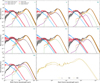 |
Fig. 5. Median SEDs of the local (U)LIRGs, separated in classes based on their merging stage. Classes ‘s’, ‘m’, and ‘M1’ are presented in the three top panels (from left to right), and classes ‘M2’, ‘M3, and ‘M4’ are presented in the three middle panels, while in the bottom-left panel the median SED of the ‘M5’ class is plotted. The curves and the shaded areas are coloured in the same manner as in Fig. 2. The bottom-right panel shows the comparison among the median SEDs of ‘s’, ‘M1’, and ‘M3’ classes, allowing for the differences to be spotted. |
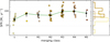 |
Fig. 6. SFR of (U)LIRGs in different merging stages, as derived from CIGALE. Each circle corresponds to an individual source. Black diamonds stand for the median values per merging class, while error bars indicate the range between the 16th and 84th percentiles from the median. Side plots of the distributions of class ‘s’, ‘M1’, and ‘M3’ systems, with the corresponding colour, are also presented. |
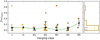 |
Fig. 7. AGN fraction of (U)LIRGs in different merging stages, as derived from CIGALE, along with distributions for the class ‘s’, ‘M1’, and ‘M3’ systems. The style of markers is the same as in Fig. 6 |
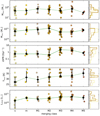 |
Fig. 8. Physical properties, as derived by CIGALE, for the seven different merging classes of (U)LIRGs. From top to the bottom, Mdust, Mstar, sSFR, Tdust, and LPDR are plotted as a function of the merging class. Each circle (following the colour coding of Fig. 6) corresponds to an individual system. Black diamonds stand for the median values per galaxy type, while the associated 16th and 84th percentile ranges are indicated with error bars. Distributions of class ‘s’, ‘M1’, and ‘M3’ systems, with the corresponding colour, are also presented as side plots. |
The change in the SFR with the merging class is visualised in Fig. 6, where the yellow-coloured circles are the values for individual sources in each sub-class with the median value indicated as black squares. The error bars bracket the 16th and 84th percentiles from the median. The green line connects the median values and indicates the general trend. The side-plots show the histograms of the SFR for the three merging classes, ‘s’, ‘M1’, and ‘M3’. We see that, although there is a large scatter in each sub-class among the different sources, there is a clear trend with the maximum median SFR occurring at sources of class ‘M4’ (99 M⊙ yr−1), followed by class ‘M3’ (93 M⊙ yr−1), with the lowest SFR at class ‘s’ (26 M⊙ yr−1) and class ‘M2’ (51 M⊙ yr−1) with the rest of the classes obtaining intermediate median values (66 M⊙ yr−1, 54 M⊙ yr−1, and 71 M⊙ yr−1, for classes ‘m’, ‘M1’, and ‘M5’, respectively). This general behaviour is to be expected since galaxies in ‘s’ and ‘M2’ classes are more relaxed systems (either separated (class ‘M2’) or totally isolated (class ‘s’)) with their SFR being mainly driven by internal processes or by past minor merging events which are not as powerful mechanisms as the tidal disruptions that take place during major merger interactions. It should be noted, however, that if the nuclear SFR is considered, as opposed to the global SFR treated here, a more obvious, increasing trend with merging stages is evident (U et al. 2019). The change in the SFR is also evident in the individual SEDs of the different sub-classes. In looking carefully at the median young-stellar SEDs in each plot of Fig. 5 (the blue curves), we see that there is an obvious enhancement of the young stellar population for class ‘M3’ and ‘M4’ systems (second and third middle panel from the left), followed by class ‘M1’ systems (top-right panel), compared to class ‘s’ and ‘M5’ systems (upper-left and bottom-left panels), which show the lowest content in young stars. This can be apparent by either comparing the maximum values of the blue curves or by comparing the relative contribution of the young and old stellar components (comparison of the blue and red curves, more evident in the MIR wavelength range). This picture is in accordance with previous studies. Already from the IRAS era, observations suggested that interactions in merging systems enhance the rate at which stars are formed (Soifer et al. 1987; Kennicutt et al. 1987). In Sanders & Mirabel (1996), the authors found a clear maximum in the IR luminosity produced by LIRGs in the stage where their nuclei merge. Similarly, Haan et al. (2011) report that LIRGs in late merging stages posses total IR luminosities larger by a factor of two than pre- or non-merging LIRGs. The median SFR per merging class, extracted from our SED modelling, follows a similar trend as the simulations suggest. Despite the large scatter in the SFR, all of the simulations seem to suggest an enhancement in the SFR close to coalescence (our merging classes ‘M3’ and ‘M4’) with lower SFRs in the other stages of the interaction where the parent galaxies are either isolated ‘s’ or apart from each other (‘M1’ and ‘M2’) or, even, systems that have been evolved to isolated galaxies (class ‘M5’). This trend is also evident when comparing the p-values of the KS tests for all combinations of the merging types (see Table D.1). If we do not consider types of ‘M5’, we see that ‘s’ types show very different distributions from all the rest giving low p-values in the SFR, while the rest of the combinations give low p-values with ‘M3’ and ‘M4’ types indicating very different distributions. The combination of ‘M3’ and ‘M4’, however, give a p-value of 0.84 suggesting very similar distributions (with a probability that they are coming from the same parent population of 84%).
The strength of the AGN in the systems of our sample, as derived by CIGALE, is presented, by merging classes in Fig. 7. We see in this plot that, although the values of the AGN fraction are in general low (≤0.2), there is a larger scatter of the values in ‘M2’ and ‘M3’ types with two of the three strongest AGNs (fracAGN > 0.6) appearing at these groups. We are aware that the AGN fraction range is limited and probably a larger sample is needed. This is also shown with the KS tests performed where all p-values in fracAGN are relatively high (see Table D.1), indicating that this parameter shows high probability that the distributions come from the same parent distribution in all combinations of merging stages. Nevertheless, our results agree with those presented in Petric et al. (2011), where they report no strong trends between the fracAGN with the merging stage, but they observe an increase in the number of AGN-dominated sources in the latest stages. In the current work, we do not find any trend between the fracAGN with the merging stage, and systems with strong AGN (fracAGN > 0.2) lie in stages later than ‘M2’ (with F13197-1627 being the only exception since it is an ‘s’ system). It is also worth noting that ‘M3’ sources exhibit lower median emission by the AGN component. This is obvious in Fig. 5, where the median AGN template is absent in this merging class, while there is an indication (given the small number of sources) of a mild dip in the median value of fracAGN of the same class of objects in Fig. 7. Springel et al. (2005) found that during the main merging event, the starburst and AGN co-exist in interacting systems. They also claim that tidal forces are able not only to trigger a nuclear starburst but also to fuel rapid growth of the black holes. Thus, although the interacting system is both starburst and AGN, it is likely that the AGN activity would be obscured by gas and dust that surrounds the nucleus. At later stages, when outflows remove the dense gas layers during the final stages of the coalescence, the remnant could be visible as an AGN. Our results, and more specifically the absence of the AGN component in class ‘M3’, may indicate a similar scenario.
Apart from the current SFR and the AGN fraction, it is interesting to investigate how other physical properties vary for galaxies of different merging stages. We do that in Fig. 8 where the change in Mdust, Mstar, sSFR, Tdust, and LPDR with the merging class is plotted (top to bottom). On the side-plots, the histograms of the parameters for three merging classes, ‘s’, ‘M1’, and ‘M3’, are also presented. The symbols are the same as in Fig. 6. Looking at the measurements of the individual systems, we see that there is a large scatter. The median values, though, suggest a few trends with the merging stage, which is worth investigating further.
The median values of Mdust suggest that this parameter remains practically unchanged with the merging stage, with median values of 5.0 × 10⁷ M⊙, 5.1 × 10⁷ M⊙, 7.7 × 10⁷ M⊙, 6.6 × 10⁷ M⊙, 4.9 × 10⁷ M⊙, 7.5 × 10⁷ M⊙, and 3.3 × 10⁷ M⊙ for merging classes ‘s’, ‘m’, and ‘M1’ to ‘M5’, respectively. From the side, the histogram plots, and also from the cumulative distributions in Appendix D, one can see that all the distributions of Mdust are very similar and well within the scatter of each individual group. This can also be confirmed by the respective p-values of the KS tests with all of them being large, for all combinations of merging stages (see Table D.1), indicating a large probability that all the distributions of the dust mass may originate from the same parent distribution.
We note that Mstar shows a mild change with objects with merging stages ‘M3’ and ‘M4’ being less massive. The median values are 6.4 × 10¹⁰ M⊙, 8.1 × 10¹⁰ M⊙, 9.3 × 10¹⁰ M⊙, 1.2 × 10¹¹ M⊙, 5.3 × 10¹⁰ M⊙, 5.3 × 10¹⁰ M⊙, and 8.1 × 10¹⁰ M⊙ for merging classes ‘s’, ‘m’, and ‘M1’ to ‘M5’. A comparison of the median SEDs in Fig. 5 suggest that class ‘M3’ and ‘M4’ systems show a deficit in the old stellar population (evident in the NIR wavelength range) compared to the rest of the merging classes (this difference is more clearly seen in the bottom-left panel of Fig. 5 by comparing the SED of ‘M3’ with the other two SEDs). This is better seen, and is discussed later, in Fig. 10 (left panel) where the histograms of the relative contribution of the old and young stellar populations are presented. The deficit of the old stars in these systems, which is responsible for the bulk of the stellar mass, results in the slightly lower stellar mass observed. This kind of trend is also confirmed by comparing the p-values of the KS tests for Mstar in Table D.1. We see that all combinations of merging stages exhibit relatively large p-values providing high probabilities that the distributions originate from the same parent distribution with the exception being the p-vales of ‘M2’ with ‘M3’ and ‘M4’, which show low values indicating very different distributions.
The clearest and most significant change, compared to the rest of the parameters examined here, is seen in the sSFR. The median values of this parameter are 0.57 Gyr−1, 0.57 Gyr−1, 0.58 Gyr−1, 0.39 Gyr−1, 2.35 Gyr−1, 1.96 Gyr−1, and 0.78 Gyr−1 for merging classes ‘s’, ‘m’, and ‘M1’ to ‘M5’, respectively. The combination of the enhanced SFR (Fig. 6) and deficit in stellar mass (Fig. 8) of classes ‘M3’ and ‘M4’ systems make these merging classes differentiate from the rest. Considering that the sSFR is a measure of the current over the past SFR suggests that these classes of objects (undergoing or having gone through a major merging event) show the most active current star-formation activity. This effect is clearly seen in the derived p-values of the KS tests with only the combinations including classes ‘M3’ and ‘M4’, showing low values indicating that their distributions substantially differ from the rest. The p-value, on the other hand, of the combination of these two merging classes is large (0.87), indicating high confidence that these two distributions are similar. This is also supported by the dust-to-stellar mass ratio that is comparable in all the merging classes 6.7 × 10⁻⁴, 8.6 × 10⁻⁴, 8.1 × 10⁻⁴, 5.9 × 10⁻⁴, 1.1 × 10⁻³, 1.2 × 10⁻³, and 4.0 × 10⁻⁴, for class ‘s’, ‘m’, and ‘M1’ to ‘M5’ objects, respectively, indicating that the variance in the star-formation activity is closer related to the merging stage rather than the stellar and dust content of the galaxies.
A mild change in the dust temperature is also obvious with the more relaxed, isolated, galaxies showing colder dust temperatures. The median dust temperatures are 27.3 K, 31.6 K, 29.5 K, 31.9 K, 32.7 K, 33.1 K, and 35.5 K for each merging class, from ‘s’ to ‘m’ and ‘M1’ to ‘M5’, respectively. The colder dust temperature that is seen in ‘s’ systems can also be explained from the SEDs. As can be seen from the lower-right panel in Fig. 5, following the merging stage evolution from ‘s’ to ‘M1’ and ‘M3’, a shift in the dust peak is obvious towards shorter wavelengths which translates to hotter temperatures. The p-values of the KS tests for the dust temperature are generally high, indicating a large probability that the distributions may originate from the same parent population (Table D.1) with only a few exceptions, mainly involving ‘M3’ and ‘M4’ merging classes.
Finally, the PDR luminosity varies slightly for different merging stages with values of 1.9 × 10¹⁰ L⊙, 3.9 × 10¹⁰ L⊙, 2.8 × 10¹⁰ L⊙, 3.5 × 10¹⁰ L⊙, 4.9 × 10¹⁰ L⊙, 5.3 × 10¹⁰ L⊙, and 4.2 × 10¹⁰ L⊙, for each merging class from ‘s’ to ‘M5’. A slight enhancement of LPDR is seen in merging classes ‘M3’ and ‘M4’ compared to the rest. This difference is more notable when comparing the distributions of ‘M2’ class systems with ‘M3’ and ‘M4’ with the p-values in the KS tests giving very small values indicating different populations.
6. Old and young stellar populations in (U)LIRGs and their role in dust heating
In Nersesian et al. (2019), the authors explored the different stellar populations in local galaxies and their role in dust heating. The SEDs of 814 galaxies of various morphological types (parametrised with their Hubble stage (T)), ranging from pure ellipticals (T = −5) to irregular galaxies (T = 10) were modelled with CIGALE, in the same way as we did with the current sample. One of the main findings of that study is that the luminosity of ETGs is dominated by the emission of the old stars with only a small contribution (maximum of ∼10% at T = 0) from young stars. For later types (T = 0–5), there is a gradual rise in the contribution of the young stars, with respect to the bolometric luminosity, reaching about 25%, while it stays roughly constant for morphological types of T > 5. In addition to that, the role of the two different stellar populations (old and young) to the dust heating was investigated for the various morphological types with Sb (T = 3) being the most efficient galaxies in the dust heating. In these galaxies, the young stars donate up to ∼77% of their luminosity to the dust heating, while this fraction is ∼24% for the old stars. In what follows, we extend their analysis to local (U)LIRGs, using exactly the same methodology, and compare them with the ‘normal’ local galaxies.
Although the use of SED modelling can provide us with useful information on the stellar populations in galaxies, it is not as robust as the use of optical spectra where the imprints of the stellar populations can be recognised in the form of various emission lines. In Rodríguez Zaurín et al. (2009), the authors use long-slit spectroscopy of 36 (U)LIRGs (with z < 0.15) to extract the relative contribution of the old and the young stellar populations. In that study, the spectra were fitted with the stellar population synthesis (SSP) models of Bruzual & Charlot (2003) in three combinations, including young stellar populations, old stellar populations, and a power-law, whenever appropriate, accounting for a possible AGN component. Their combination, including a young stellar population (tYSP ≤ 2 Gyr) and an old stellar population with an age of 12.5 Gyr, is the one that better mimics the parametrisation used of our approach. This allows for a comparison between the two methods (SED modelling and optical spectroscopy) on the derivation of the stellar populations. The fractions of the young stellar populations of the seven sources in common between the two samples (F08572+3915, F12112+0305, F12540+5708, F13428+5608, F14348-1447, F15327+2340, and F22491-1808) are shown in Fig. 9, where the ones derived from the spectra (YSPspectra) and those derived from CIGALE (YSPCIGALE) are compared. Since YSPspectra was extracted from several positions in each system, the mean value is considered, while the minimum and maximum values of YSPspectra define the uncertainty in this value (the error bars in the plot). From this plot we see that, although the scatter is large and also the uncertainty in each source is large, there is a clear trend of the sources lining up (within the errors) the one-to-one line (with the exception of F13428+5608, which, considering only the central 5kpc aperture, and neglecting the outer apertures including its long tidal tail, results in a YSPspectra of 75%, which is much closer to the value of 83% derived by CIGALE). This indicates that the values derived from the two methods are comparable, given the very different approaches. Furthermore, the median values of the two samples are also rather comparable. For the 36 (U)LIRGs in the sample of Rodríguez Zaurín et al. (2009), the median value for the young stellar population is 74 ± 13 %, while, for the 67 sources in our sample, this fraction is 64 ± 18 %.
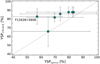 |
Fig. 9. Comparison of the fraction of the young stellar population in seven systems in common between the sample studied here (YSPCIGALE) and the sample of Rodríguez Zaurín et al. (2009). In Rodríguez Zaurín et al. (2009), the young stellar populations (YSPspectra) were derived through spectral synthesis population modelling of optical long-slit spectra (see the text for more details). |
The different stellar populations (old and young) in our systems are presented and compared with the local ‘normal’ galaxies in Fig. 10. In the left panel of Fig. 10, the histograms of the unattenuated luminosities of both stellar components to the bolometric luminosity of each galaxy ( and
and  , where
  ) are plotted. In this plot, the red and blue histograms indicate the mean values of
  and
and  , respectively. In the leftmost sub-panel, the relative contribution of the young and old stellar populations in ETGs, LTGs, and (U)LIRGs are compared, while these values for each of the seven merging sub-classes of the (U)LIRGs sample are indicated in the rightmost sub-panel. The exact numbers are presented in Table 4. The most striking feature from this plot is the large increase in
  for (U)LIRGs compared to local ETGs and LTGs. As already stated in Nersesian et al. (2019), the old stars are the prominent luminosity source in ETGs and LTGs (with mean values of
  being 96% and 79% respectively), while this picture is the opposite in the case of (U)LIRGs with 64% of their bolometric luminosity originating from young stars. This increase (by a factor of ∼3) in the luminosity of the young stellar component is, of course, the result of the intense star formation that takes place in these systems, which is mostly due to merging events. The fraction of the young stars in all seven merging sub-classes stays around the mean value of 64%, but it is class ‘M3’ and ‘M4’ systems that show the highest fraction (72% and 79%, respectively) of young stars following the trend in the SFR (Fig. 6). All the related values are given in Table 4.
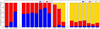 |
Fig. 10. Left panel: contribution of the old (red) and young (blue) stellar populations to the unattenuated luminosity, over the bolometric luminosity, per galaxy type and (U)LIRGs merging class. Right panel: contribution of the old and young stellar populations to the attenuated luminosity, over the bolometric luminosity, per galaxy type and (U)LIRGs merging class (same colours as in left panel), together with the ratio of the dust luminosity to the bolometric luminosity (yellow). |
Mean values of the ratios of various combinations of the stellar and dust luminosity components extracted using the CIGALE SED fitting tool. These ratios are presented for the three general galaxy populations compared in this study (ETGs, LTGs, and (U)LIRGs), as well as for the seven merging classes of (U)LIRGs.
The right panel in Fig. 10 shows the effects of dust in the stellar populations discussed previously. Here, the ratio of the dust-attenuated luminosity of the old stellar population ( ) and of the young stellar population (
 ) to the bolometric luminosity is plotted with red and blue colours, respectively, while the fraction of the dust-absorbed luminosity (fabs; see also Sect. 4.2) is indicated with a yellow colour. The leftmost sub-panel shows the comparison of these quantities for ETGs, LTGs, and (U)LIRGs, while the rightmost sub-panel shows the comparison among the different merging sub-classes. What is evident from this plot is the large effect that dust has on the energy budget of (U)LIRGs compared to ETGs and LTGs. We note that fabs changes from very low (7%) for ETGs, to moderate (25%) for LTGs, to very high (78%) for (U)LIRGs. This can be mainly explained by the higher dust mass that is detected in (U)LIRGs (upper panel in Fig. 4) and, especially, the dust associated with the PDR regions (bottom panel in Fig. 4). The dramatic effect of the dust on the stellar populations is clearly seen by comparing the leftmost sub-panels of each panel in Fig. 10. For (U)LIRGs, we see that the fraction of the young stars is absorbed so heavily that it goes from 64% in the unattenuated case to 5% in the case where absorption by dust is considered. It is also worth mentioning that the attenuated fraction of the luminosity of the young stars is higher for LTGs (9%) compared to 2% and 5% in ETGs and (U)LIRGs. Class ‘M3’ and ‘M4’ systems show the highest mean fabs values (84% and 87%, respectively), with classes ‘s’ and ‘M2’ having the lowest mean fabs values (73%). All the related values are given in Table 4.
As has already been discussed above, a large fraction of the energy emitted by the stars in (U)LIRGs is absorbed by the dust grains (see the right panel in Fig. 10), resulting in their heating and the production of large amounts of IR radiation in those systems. With our analysis, we can not only quantify the total stellar radiation that is absorbed by the dust, but we can also distinguish between the two stellar populations and calculate their efficiency in heating up the dust grains. The quantity that shows the fraction of each stellar population that is absorbed by the dust is the ratio of the absorbed luminosity of each stellar component to the respective unattenuated stellar component ( and
and  for the old and the young stellar component, respectively). The remaining luminosity (not absorbed by the dust) is the attenuated luminosity of each stellar component, which, when divided by the unattenuated luminosity, gives the fraction of the luminosity that is unaffected by the dust (
 and
and  for the old and the young stellar component, respectively). For each stellar population, the crossed bars in Fig. 11 show the mean values of the absorbed fraction of the luminosity, which contributes to the dust heating (
 ), while the rest, which are shown with solid bars, are the fraction of the luminosity emitted by stars, without being affected by the dust (
 ). The left panel shows the different contributions of the old stars (red colour) and the right panel shows those of the young stars (blue colour) for each galaxy population (ETGs, LTGs, and (U)LIRGs in the leftmost sub-panels) and for each merging class (rightmost sub-panels). Looking at the different galaxy types, it is evident that it is the young stellar component that offers the larger portion of its total luminosity in the dust heating compared to the old one. In particular, for ETGs, 30% of the young stellar luminosity donated to the dust heating compared to only 6% for the old stars, while in LTGs these fractions are 58% and 17% and they get extremely high in (U)LIRGs (92% and 56% for the young and the old stellar populations, respectively). It is noteworthy that even the old stars in (U)LIRGs have a significant role in the dust heating contributing with more than half of their luminosities. The mean values of the fractions of the dust-absorbed luminosity for each of the two stellar components have comparable values for the four merging classes with no significant deviations (see the rightmost sub-panels in Fig. 11). All the related values are summarised in Table 4.
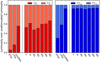 |
Fig. 11. Mean values of the fraction of the luminosity of the old and the young stellar populations (left and right panel, respectively) used for the dust heating. The crossed bars show the mean values of the ratio of the dust-absorbed luminosity to the unattenuated luminosity of the corresponding stellar component, while the solid bars are the ratios of the attenuated luminosity of the specific stellar component to its unattenuated luminosity. In each panel, the ratios are presented for each of the three galaxy populations (ETGs, LTGs, and (U)LIRGs) in the leftmost sub-panel, and for the four merging classes in the rightmost sub-panel. |
It is also interesting to investigate the relative contribution of the stellar populations to the dust heating. The parameter that indicates this contribution is the ratio of the dust-absorbed luminosity, for each stellar population, to the total dust luminosity ( and
and  for the old and the young stars, respectively). The histograms of the mean values of this parameter are presented in Fig. 12 with red and blue colours representing the contribution of the old and the young stellar components, respectively. In this plot, these contributions in ETGs, LTGs, and (U)LIRGs are plotted in the leftmost part, while the rightmost part shows the relative contribution for the four merging classes. For ETGs, as already described in Nersesian et al. (2019), it is mainly the old stars that contribute more to the dust heating (by 86%), while in LTGs both the old and the young stars contribute almost equally to the dust heating (52% for the old stellar population). In (U)LIRGs, the picture reverses with the young stars taking over the heating of the dust grains with 74% of the luminosity of this stellar population absorbed by dust.
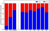 |
Fig. 12. Mean values of the ratios of the dust-absorbed stellar luminosity (originating from old and young stars) to the dust luminosity (red and blue colours, respectively). The ratios are presented for each of the three galaxy populations (ETGs, LTGs, and (U)LIRGs) in the leftmost sub-panel and for the four merging classes in the rightmost sub-panel. |
It is also interesting to investigate the relative contribution of the stellar populations to the dust heating. The parameter that indicates this contribution is the ratio of the dust-absorbed luminosity, for each stellar population, to the total dust luminosity ( and
and  for the old and the young stars, respectively). The histograms of the mean values of this parameter are presented in Fig. 12 with red and blue colours representing the contribution of the old and the young stellar components, respectively. In this plot, these contributions in ETGs, LTGs, and (U)LIRGs are plotted in the leftmost part, while the rightmost part shows the relative contribution for the four merging classes. For ETGs, as already described in Nersesian et al. (2019), it is mainly the old stars that contribute more to the dust heating (by 86%), while in LTGs both the old and the young stars contribute almost equally to the dust heating (52% for the old stellar population). In (U)LIRGs the picture reverses with the young stars taking over the heating of the dust grains with 74% of the luminosity of this stellar population absorbed by dust.
Concerning the relative contribution of the two stellar populations to the dust heating of the different merging classes, we see that it remains close to the mean value of (U)LIRGs (74% for the young stars) with only small deviations. The largest deviations for the contribution of the young stars to the dust heating are found between classes ‘s’ and ‘m’ (65% and 67%) and classes ‘M3’ and ‘M4’ (80% and 85%), respectively. All the related values are summarised in Table 4.
7. Summary
In this study, we have modelled the SEDs of 67 local (U)LIRGs, using the CIGALE code, to calculate their physical properties. Their stellar mass, dust mass, star-formation rate, dust temperature, as well as their luminosity arising from PDR regions were derived and compared to those of 268 ETGs and 542 LTGs (already derived in a similar way in Nersesian et al. 2019). Furthermore, the (U)LIRGs are categorised in seven classes according to their merging stage (ranging from totally isolated to pre-mergers, mergers, and post-mergers), providing useful information on how their properties depend on the phase of the interaction of the parent galaxies. Finally, the contribution of the two stellar populations (old and young) to the bolometric luminosity of these systems and their role in the dust heating is also explored. Our findings are summarised as follows:
-
(U)LIRGs occupy the ‘high-end’ on the Mdust, Mstar, and SFR plane in the local Universe compared to ETGs and LTGs (with the corresponding parameters already calculated in Nersesian et al. 2019). Their median dust mass is 5.2 × 10⁷ M⊙ compared to 4.6 × 10⁵ M⊙ and 5 × 10⁶ M⊙ for ETGs and LTGs, respectively. Their median stellar mass is 6.3 × 10¹⁰ M⊙ compared to 1.5 × 10¹⁰M⊙ and 4.2 × 10⁹ M⊙ for ETGs and LTGs, respectively. The SFR in (U)LIRGs gets a much higher median value of 52.0 M⊙ yr−1 compared to 0.01, and 0.4 M⊙ yr−1 for ETGs and LTGs, respectively. The median values of the specific sSFR, on the other hand, ranges from 7 × 10⁻⁴ and 0.1 Gyr−1 for ETGs and LTGs to 1.0 Gyr−1 for (U)LIRGs, respectively. These differences among the three galaxy populations in the local Universe can also be traced by carefully examining their median SEDs.
-
The median SEDs show a slight shift in the wavelength axis of the dust emission peak, indicating that the dust temperature is cooler in LTGs and warmer in (U)LIRGs with median dust temperatures of 28, 22, and 32 K for ETGs, LTGs, and (U)LIRGs, respectively. The SEDs also reveal the significance of the dust emission in PDR regions increasing from ETGs to LTGs to (U)LIRGs with the median values of the ratios of the PDR-to-total dust luminosity changing from 1.6%, to 5.2%, to 11.7%, respectively. Furthermore, the attenuation effects, caused by the dust, are evident in the median SEDs with the peak of the stellar emission (measured at 1 μm) being the highest for ETGs, slightly lower (by 0.23 dex) for LTGs, and much lower (by 1.95 dex) for (U)LIRGs (compared to ETGs). A comparison of the attenuated and unattenuated curves of the SEDs indicates that the attenuation by the dust becomes significant short-wards of ∼0.2 μm, ∼1 μm, and ∼2 μm for ETGs, LTGs, and (U)LIRGs, respectively.
-
Small differences in the derived parameters are seen for the seven merging classes of our sample of (U)LIRGs. The dust mass is very similar among different merging classes, within the scatter of the measurements, while a mild deficit is seen in the stellar mass for class ‘M3’ and ‘M4’ objects. The most evident change is seen in the SFR with the median values computed for class ‘M4’ objects being the highest (99 M⊙ yr−1) followed by class ‘M3’ (93 M⊙ yr−1), with the lowest SFR occurring at class ‘s’ (26 M⊙ yr−1) sources. A mild change in the dust temperature is found with an increasing trend of the median value from 27.3 K to 35.5 K from the isolated to the more evolved systems respectively. The PDR luminosity is slightly enhanced for classes ‘M3’ and ‘M4’ systems, compared to the rest of the classes, which is consistent with the higher SFR observed in those systems.
-
In contrast to the local ‘normal’ galaxies where the old stars are the dominant source of the stellar emission (with the fraction of their luminosity over the bolometric luminosity being 96% and 79% for ETGs and LTGs, respectively), this picture reverses in (U)LIRGs with the young stars being the dominant source of stellar emission with the fraction of their luminosity being 64% of the bolometric one. Out of the seven merging classes, classes ‘M4’ and ‘M3’ show the highest such contribution (79% and 72%, respectively). The effects of dust in (U)LIRGs, parametrised by the dust-absorbed luminosity, to the bolometric luminosity is extremely high (78%) compared to 7% and 25% in ETGs and LTGs, respectively.
-
The fraction of the stellar luminosity used to heat up the dust grains is very high in (U)LIRGs for both stellar components (92% and 56% for young and old, respectively), compared to 30% and 6% for ETGs and 58% and 17% for LTGs, respectively. In (U)LIRGs 74% of the dust heating comes from the young stars, with the old stars being the dominant source of dust heating contributing with 86% in ETGs and 52% in LTGs.
The analysis described here complements that of Nersesian et al. (2019), shedding light on the global properties of galaxies in the local Universe. Focusing on the stellar populations and their role in the dust heating, local (U)LIRGs are found to be dominated by young stars which constitute the main heating source of the dust residing in such systems. The way that stellar populations in galaxies and their efficiency in heating dust grains evolve with redshift is something that we plan to address in future studies.
Acknowledgments
We would like to thank the anonymous referee for providing comments and suggestions, which helped to improve the quality of the manuscript. This research is co-financed by Greece and the European Union (European Social Fund-ESF) through the Operational Programme “Human Resources Development, Education and Lifelong Learning 2014–2020” in the context of the project “Anatomy of galaxies: their stellar and dust content through cosmic time” (MIS 5052455). GM acknowledges support by the Agencia Estatal de Investigación, Unidad de Excelencia María de Maeztu, ref. MDM-2017-0765. DustPedia is a collaborative focused research project supported by the European Union under the Seventh Framework Programme (2007–2013) call (proposal no. 606847). The participating institutions are: Cardiff University, UK; National Observatory of Athens, Greece; Ghent University, Belgium; Université Paris Sud, France; National Institute for Astrophysics, Italy and CEA, France. This research has made use of the NASA/IPAC Extragalactic Database (NED), which is operated by the Jet Propulsion Laboratory, California Institute of Technology, under contract with the National Aeronautics and Space Administration. We have also made use of the VizieR catalogue access tool, CDS, Strasbourg, France (DOI : 10.26093/cds/vizier). The original description of the VizieR service was published in A&AS 143, 23.
References
- Aniano, G., Draine, B. T., Calzetti, D., et al. 2012, ApJ, 756, 138 [NASA ADS] [CrossRef] [Google Scholar]
- Armus, L., Heckman, T., & Miley, G. 1987, AJ, 94, 831 [NASA ADS] [CrossRef] [Google Scholar]
- Armus, L., Mazzarella, J. M., Evans, A. S., et al. 2009, PASP, 121, 559 [Google Scholar]
- Baes, M., Verstappen, J., De Looze, I., et al. 2011, ApJS, 196, 22 [NASA ADS] [CrossRef] [Google Scholar]
- Bianchi, S., De Vis, P., Viaene, S., et al. 2018, A&A, 620, A112 [NASA ADS] [CrossRef] [EDP Sciences] [Google Scholar]
- Bongiorno, A., Merloni, A., Brusa, M., et al. 2012, MNRAS, 427, 3103 [NASA ADS] [CrossRef] [Google Scholar]
- Boquien, M., Boselli, A., Buat, V., et al. 2013, A&A, 554, A14 [NASA ADS] [CrossRef] [EDP Sciences] [Google Scholar]
- Boquien, M., Burgarella, D., Roehlly, Y., et al. 2019, A&A, 622, A103 [NASA ADS] [CrossRef] [EDP Sciences] [Google Scholar]
- Brinchmann, J., Charlot, S., White, S. D. M., et al. 2004, MNRAS, 351, 1151 [NASA ADS] [CrossRef] [Google Scholar]
- Bruzual, G., & Charlot, S. 2003, MNRAS, 344, 1000 [NASA ADS] [CrossRef] [Google Scholar]
- Calzetti, D., Armus, L., Bohlin, R. C., et al. 2000, ApJ, 533, 682 [NASA ADS] [CrossRef] [Google Scholar]
- Camps, P., & Baes, M. 2015, Astron. Comput., 9, 20 [NASA ADS] [CrossRef] [Google Scholar]
- Casey, C. M. 2012, MNRAS, 425, 3094 [Google Scholar]
- Chabrier, G. 2003, PASP, 115, 763 [Google Scholar]
- Chang, Y.-Y., van der Wel, A., da Cunha, E., & Rix, H.-W. 2015, ApJS, 219, 8 [NASA ADS] [CrossRef] [Google Scholar]
- Charlot, S., & Fall, S. M. 2000, ApJ, 539, 718 [Google Scholar]
- Chu, J. K., Sanders, D. B., Larson, K. L., et al. 2017, ApJS, 229, 25 [Google Scholar]
- Ciesla, L., Boselli, A., Elbaz, D., et al. 2016, A&A, 585, A43 [NASA ADS] [CrossRef] [EDP Sciences] [Google Scholar]
- Ciesla, L., Charmandaris, V., Georgakakis, A., et al. 2015, A&A, 576, A10 [NASA ADS] [CrossRef] [EDP Sciences] [Google Scholar]
- Clark, C. J. R., Verstocken, S., Bianchi, S., et al. 2018, A&A, 609, A37 [NASA ADS] [CrossRef] [EDP Sciences] [Google Scholar]
- Clements, D. L., Sutherland, W. J., McMahon, R. G., & Saunders, W. 1996, MNRAS, 279, 477 [NASA ADS] [CrossRef] [Google Scholar]
- Cox, T. J., Jonsson, P., Primack, J. R., & Somerville, R. S. 2006, MNRAS, 373, 1013 [NASA ADS] [CrossRef] [Google Scholar]
- da Cunha, E., Charmandaris, V., Díaz-Santos, T., et al. 2010a, A&A, 523, A78 [NASA ADS] [CrossRef] [EDP Sciences] [Google Scholar]
- da Cunha, E., Eminian, C., Charlot, S., & Blaizot, J. 2010b, MNRAS, 403, 1894 [NASA ADS] [CrossRef] [Google Scholar]
- Dale, D. A., Helou, G., Magdis, G. E., et al. 2014, ApJ, 784, 83 [NASA ADS] [CrossRef] [Google Scholar]
- Davies, J. I., Baes, M., Bianchi, S., et al. 2017, PASP, 129 [Google Scholar]
- Davies, J. I., Nersesian, A., Baes, M., et al. 2019, A&A, 626, A63 [CrossRef] [EDP Sciences] [Google Scholar]
- Di Matteo, P., Bournaud, F., Martig, M., et al. 2008, A&A, 492, 31 [NASA ADS] [CrossRef] [EDP Sciences] [Google Scholar]
- Díaz-Santos, T., Armus, L., Charmandaris, V., et al. 2017, ApJ, 846, 32 [Google Scholar]
- Duc, P. A., Brinks, E., Wink, J. E., & Mirabel, I. F. 1997, A&A, 326, 537 [Google Scholar]
- Dunne, L., & Eales, S. A. 2001, MNRAS, 327, 697 [NASA ADS] [CrossRef] [Google Scholar]
- Dunne, L., Eales, S., Edmunds, M., et al. 2000, MNRAS, 315, 115 [NASA ADS] [CrossRef] [Google Scholar]
- Elbaz, D., Daddi, E., Le Borgne, D., et al. 2007, A&A, 468, 33 [NASA ADS] [CrossRef] [EDP Sciences] [Google Scholar]
- Elvis, M., Hao, H., Civano, F., et al. 2012, ApJ, 759, 6 [NASA ADS] [CrossRef] [Google Scholar]
- Fritz, J., Franceschini, A., & Hatziminaoglou, E. 2006, MNRAS, 366, 767 [Google Scholar]
- Gao, Y., Lo, K. Y., Lee, S. W., & Lee, T. H. 2001, ApJ, 548, 172 [NASA ADS] [CrossRef] [Google Scholar]
- Genzel, R., Lutz, D., Sturm, E., et al. 1998, ApJ, 498, 579 [NASA ADS] [CrossRef] [Google Scholar]
- Giovannoli, E., Buat, V., Noll, S., Burgarella, D., & Magnelli, B. 2011, A&A, 525, A150 [NASA ADS] [CrossRef] [EDP Sciences] [Google Scholar]
- Haan, S., Surace, J. A., Armus, L., et al. 2011, AJ, 141, 100 [NASA ADS] [CrossRef] [Google Scholar]
- Hainline, L. J., Blain, A. W., Smail, I., et al. 2011, ApJ, 740, 96 [Google Scholar]
- Herrero-Illana, R., Privon, G. C., Evans, A. S., et al. 2019, A&A, 628, A71 [EDP Sciences] [Google Scholar]
- Hollenbach, D. J., & Tielens, A. G. G. M. 1999, Rev. Mod. Phys., 71, 173 [Google Scholar]
- Hopkins, P. F., Cox, T. J., Hernquist, L., et al. 2013, MNRAS, 430, 1901 [Google Scholar]
- Hutchings, J. B., & Neff, S. G. 1991, AJ, 101, 434 [NASA ADS] [CrossRef] [Google Scholar]
- Ichikawa, K., Ueda, Y., Terashima, Y., et al. 2012, ApJ, 754, 45 [NASA ADS] [CrossRef] [Google Scholar]
- Ishida, C. M. 2004, PhD Thesis, University of Hawai’I [Google Scholar]
- Iwasawa, K., Sanders, D. B., Teng, S. H., et al. 2011, A&A, 529, A106 [NASA ADS] [CrossRef] [EDP Sciences] [Google Scholar]
- Johnston, R., Vaccari, M., Jarvis, M., et al. 2015, MNRAS, 453, 2540 [NASA ADS] [CrossRef] [Google Scholar]
- Jones, A. P., Köhler, M., Ysard, N., Bocchio, M., & Verstraete, L. 2017, A&A, 602, A46 [NASA ADS] [CrossRef] [EDP Sciences] [Google Scholar]
- Kennicutt, R. C., Keel, W. C., van der Hulst, J. M., Hummel, E., & Roettiger, K. A. 1987, AJ, 93, 1011 [NASA ADS] [CrossRef] [Google Scholar]
- Kennicutt, R. C., Schweizer, F., & Barnes, J. E. 1996, Galaxies: Interactions and Induced Star Formation [Google Scholar]
- Kilerci Eser, E., Goto, T., & Doi, Y. 2014, ApJ, 797, 54 [NASA ADS] [CrossRef] [Google Scholar]
- Kim, D. C., Evans, A. S., Vavilkin, T., et al. 2013, ApJ, 768, 102 [Google Scholar]
- Larson, R. B., & Tinsley, B. M. 1978, ApJ, 219, 46 [NASA ADS] [CrossRef] [Google Scholar]
- Larson, K. L., Sanders, D. B., Barnes, J. E., et al. 2016, ApJ, 825, 128 [NASA ADS] [CrossRef] [Google Scholar]
- Lawrence, A., Rowan-Robinson, M., Leech, K., Jones, D. H. P., & Wall, J. V. 1989, MNRAS, 240, 329 [NASA ADS] [Google Scholar]
- Leech, K. J., Rowan-Robinson, M., Lawrence, A., & Hughes, J. D. 1994, MNRAS, 267, 253 [NASA ADS] [CrossRef] [Google Scholar]
- Lonsdale, C. J., Farrah, D., & Smith, H. E. 2006, in Ultraluminous Infrared Galaxies, ed. J. W. Mason, 285 [Google Scholar]
- Lyu, J., & Rieke, G. H. 2018, ApJ, 866, 92 [NASA ADS] [CrossRef] [Google Scholar]
- Madau, P., & Dickinson, M. 2014, ARA&A, 52, 415 [NASA ADS] [CrossRef] [Google Scholar]
- Magdis, G. E., Daddi, E., Béthermin, M., et al. 2012, ApJ, 760, 6 [NASA ADS] [CrossRef] [Google Scholar]
- Makarov, D., Prugniel, P., Terekhova, N., Courtois, H., & Vauglin, I. 2014, A&A, 570, A13 [CrossRef] [EDP Sciences] [Google Scholar]
- Małek, K., Pollo, A., Takeuchi, T. T., et al. 2014, A&A, 562, A15 [NASA ADS] [CrossRef] [EDP Sciences] [Google Scholar]
- Melnick, J., & Mirabel, I. F. 1990, A&A, 231, L19 [NASA ADS] [Google Scholar]
- Morrissey, P., Conrow, T., Barlow, T. A., et al. 2007, ApJS, 173, 682 [Google Scholar]
- Mountrichas, G., Buat, V., Yang, G., et al. 2021, A&A, 646, A29 [EDP Sciences] [Google Scholar]
- Nardini, E., Risaliti, G., Watabe, Y., Salvati, M., & Sani, E. 2010, MNRAS, 405, 2505 [NASA ADS] [Google Scholar]
- Nersesian, A., Xilouris, E. M., Bianchi, S., et al. 2019, A&A, 624, A80 [NASA ADS] [CrossRef] [EDP Sciences] [Google Scholar]
- Nikutta, R., Elitzur, M., & Lacy, M. 2009, ApJ, 707, 1550 [NASA ADS] [CrossRef] [Google Scholar]
- Noll, S., Burgarella, D., Giovannoli, E., et al. 2009, A&A, 507, 1793 [NASA ADS] [CrossRef] [EDP Sciences] [Google Scholar]
- Pappalardo, C., Bizzocchi, L., Fritz, J., et al. 2016, A&A, 589, A11 [NASA ADS] [CrossRef] [EDP Sciences] [Google Scholar]
- Pearson, W. J., Wang, L., Hurley, P. D., et al. 2018, A&A, 615, A146 [NASA ADS] [CrossRef] [EDP Sciences] [Google Scholar]
- Petric, A. O., Armus, L., Howell, J., et al. 2011, ApJ, 730, 28 [NASA ADS] [CrossRef] [Google Scholar]
- Pilbratt, G. L., Riedinger, J. R., Passvogel, T., et al. 2010, A&A, 518, L1 [CrossRef] [EDP Sciences] [Google Scholar]
- Ramos, P. A. F., Ashby, M. L. N., Smith, H. A., et al. 2020, MNRAS, 499, 4369 [Google Scholar]
- Renaud, F., Bournaud, F., & Duc, P.-A. 2015, MNRAS, 446, 2038 [NASA ADS] [CrossRef] [Google Scholar]
- Ricci, C., Bauer, F. E., Treister, E., et al. 2017, MNRAS, 468, 1273 [NASA ADS] [Google Scholar]
- Rodríguez Zaurín, J., Tadhunter, C. N., & González Delgado, R. M. 2009, MNRAS, 400, 1139 [NASA ADS] [CrossRef] [Google Scholar]
- Roehlly, Y., Burgarella, D., Buat, V., et al. 2014, in Astronomical Data Analysis Software and Systems XXIII, eds. N. Manset, P. Forshay, et al., ASP Conf. Ser., 485, 347 [Google Scholar]
- Salim, S., Boquien, M., & Lee, J. C. 2018, ApJ, 859, 11 [NASA ADS] [CrossRef] [Google Scholar]
- Salpeter, E. E. 1955, ApJ, 121, 161 [Google Scholar]
- Sanders, D. B., & Mirabel, I. F. 1996, ARA&A, 34, 749 [NASA ADS] [CrossRef] [Google Scholar]
- Sanders, D. B., Mazzarella, J. M., Kim, D. C., Surace, J. A., & Soifer, B. T. 2003, AJ, 126, 1607 [Google Scholar]
- Schreiber, C., Pannella, M., Elbaz, D., et al. 2015, A&A, 575, A74 [NASA ADS] [CrossRef] [EDP Sciences] [Google Scholar]
- Schweizer, F., & Seitzer, P. 1992, AJ, 104, 1039 [NASA ADS] [CrossRef] [Google Scholar]
- Skrutskie, M. F., Cutri, R. M., Stiening, R., et al. 2006, AJ, 131, 1163 [NASA ADS] [CrossRef] [Google Scholar]
- Smirnov, N. 1948, Ann. Math. Statist., 19, 279 [Google Scholar]
- Soifer, B. T., Neugebauer, G., & Houck, J. R. 1987, ARA&A, 25, 187 [NASA ADS] [CrossRef] [Google Scholar]
- Spearman, C. 1904, Am. J. Psychol., 15, 72 [Google Scholar]
- Springel, V., Di Matteo, T., & Hernquist, L. 2005, MNRAS, 361, 776 [Google Scholar]
- Stalevski, M., Fritz, J., Baes, M., Nakos, T., & Popović, L. Č. 2012, MNRAS, 420, 2756 [NASA ADS] [CrossRef] [Google Scholar]
- Stalevski, M., Ricci, C., Ueda, Y., et al. 2016, MNRAS, 458, 2288 [NASA ADS] [CrossRef] [Google Scholar]
- Stalevski, M., Asmus, D., & Tristram, K. R. W. 2017, MNRAS, 472, 3854 [NASA ADS] [CrossRef] [Google Scholar]
- Stalevski, M., Tristram, K. R. W., & Asmus, D. 2019, MNRAS, 484, 3334 [NASA ADS] [CrossRef] [Google Scholar]
- Stierwalt, S., Armus, L., Surace, J. A., et al. 2013, ApJS, 206, 1 [NASA ADS] [CrossRef] [Google Scholar]
- Struck, C. 2006, in Galaxy Collisions—Dawn of a New Era, ed. J. W. Mason, 115 [Google Scholar]
- Tanimoto, A., Ueda, Y., Odaka, H., et al. 2019, ApJ, 883, 110 [Google Scholar]
- Tinsley, B. M. 1968, ApJ, 151, 547 [NASA ADS] [CrossRef] [Google Scholar]
- Toomre, A., & Toomre, J. 1972, ApJ, 178, 623 [Google Scholar]
- Torres-Albà, N., Iwasawa, K., Díaz-Santos, T., et al. 2018, A&A, 620, A140 [NASA ADS] [CrossRef] [EDP Sciences] [Google Scholar]
- U, V., Medling, A. M., Inami, H., et al. 2019, ApJ, 871, 166 [CrossRef] [Google Scholar]
- U, V., Sanders, D. B., Mazzarella, J. M., et al. 2012, ApJS, 203, 9 [NASA ADS] [CrossRef] [Google Scholar]
- Vika, M., Ciesla, L., Charmandaris, V., Xilouris, E. M., & Lebouteiller, V. 2017, A&A, 597, A51 [NASA ADS] [CrossRef] [EDP Sciences] [Google Scholar]
- Werner, M. W., Roellig, T. L., Low, F. J., et al. 2004, ApJS, 154, 1 [NASA ADS] [CrossRef] [Google Scholar]
- Whitaker, K. E., van Dokkum, P. G., Brammer, G., & Franx, M. 2012, ApJ, 754, L29 [NASA ADS] [CrossRef] [Google Scholar]
- Whitaker, K. E., Franx, M., Leja, J., et al. 2014, ApJ, 795, 104 [NASA ADS] [CrossRef] [MathSciNet] [Google Scholar]
- Wuyts, S., Franx, M., Cox, T. J., et al. 2009, ApJ, 696, 348 [NASA ADS] [CrossRef] [Google Scholar]
- Wuyts, S., Förster Schreiber, N. M., Lutz, D., et al. 2011a, ApJ, 738, 106 [NASA ADS] [CrossRef] [Google Scholar]
- Wuyts, S., Förster Schreiber, N. M., van der Wel, A., et al. 2011b, ApJ, 742, 96 [NASA ADS] [CrossRef] [Google Scholar]
- Yang, G., Boquien, M., Buat, V., et al. 2020, MNRAS, 491, 740 [NASA ADS] [CrossRef] [Google Scholar]
- Zou, Z., Xia, X., Deng, Z., & Su, H. 1991, MNRAS, 252, 593 [Google Scholar]
Appendix A: CIGALE validation (mock analysis)
In order to examine how well the derived parameters can be constrained from the multi-wavelength SED fitting that CIGALE performs, and to monitor the accuracy and precision expected for each parameter, we made use of the CIGALE module that performs a mock analysis. This module creates a mock SED for each galaxy based on the best fitted parameters, allowing the fluxes to vary within the uncertainties of the observations by adding a value taken from a Gaussian distribution with the same standard deviation as indicated by the observations. By modelling these mock SEDs with CIGALE, we can then retrieve the best set of the mock fitted parameters and compare them with those used as input. This provides us with a direct measure of how accurately one can retrieve specific parameters for a specific sample of galaxies.
The results of the mock analysis are presented in Fig. A.1 with the best fitted values of each parameter (input values; x-axis) compared to the mock values of the each parameter (mock values; y-axis). The red circles indicate the strongest AGNs in the sample with fracAGN > 0.2. The solid blue line corresponds to the one-to-one relation, while the orange dashed line corresponds to the best linear fit to the data. The relevant value of the Spearman’s correlation coefficient (ρ) is also indicated in each panel.
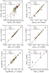 |
Fig. A.1. Best fitted parameters (input values; x-axis) versus the mock parameters (mock values; y-axis) as derived by the mock analysis performed with CIGALE. Each circle corresponds to an individual galaxy with the red circles indicating the strongest AGNs in the sample with fracAGN > 0.2. The solid blue line corresponds to the one-to-one relation, while the orange dashed line corresponds to the best linear fit to the data. The relevant value of the Spearman’s correlation coefficient (ρ) is also indicated in each panel. |
The parameters presented in the mock analysis are the ones used in this work or they have been used for the calculation of other quantities (e.g., Umin for the calculation of Tdust). It is evident that all the mock-derived values have a strong correlation with the input parameters with the Spearman’s correlation coefficient being more than ∼0.9 in all cases. This indicates that CIGALE can adequately calculate the true value well. The only exception is with the calculation of Umin showing some deviant points, especially for galaxies with strong AGNs, but, overall, the input and mock data are in a good agreement with ρ = 0.92.
Appendix B: Best-fit SED models
The SEDs of the 67 (U)LIRGs analysed in this study are presented here. The goodness of the fit for each source is indicated with the reduced χ2 of the fit listed in Table 3. For a few exceptional cases, for example, F12224-0624, F15107+0724, and F15327+2340, CIGALE gives a poor fit close to the FIR peak resulting in relatively large reduced χ2 values. This may have some effect on derived dust parameters for these systems.
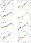 |
Fig. B.1. Best-fit SED models for the 67 galaxies in the current sample containing the unattenuated emission by the old (red) and the young (blue) stellar populations, the nebular line emission (dark-yellow), the diffuse dust (orange), the emission from the PDR regions (green), as well as the AGN emission (purple) are also presented. The best-fit SED is indicated as a black curve, while the observations for each galaxy, along with their uncertainties, are indicated by violet open squares. Light-green dots stand for the best-model flux densities. |
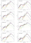 |
Fig. B.1. continued. |
 |
Fig. B.1. continued. |
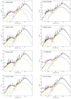 |
Fig. B.1. continued. |
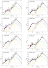 |
Fig. B.1. continued. |
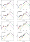 |
Fig. B.1. continued. |
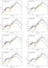 |
Fig. B.1. continued. |
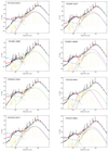 |
Fig. B.1. continued. |
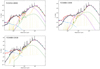 |
Fig. B.1. continued. |
Appendix C: Comparison with other studies
The (U)LIRGs sample under consideration has already been studied by others and some of the physical parameters discussed in this paper have been computed using either a similar approach or a totally different methodology. In what follows, we compare the parameters provided in the literature with what is computed in the current work and try to explain any differences.
The AGN is inevitably a very important contributor to the energetics of the galaxies which can shape a large part of their SED (at least for the galaxies that host strong AGNs). The contribution of this component can be parametrised by the fraction of its emitted luminosity to the bolometric luminosity emitted. This fraction (fracAGN) can be estimated with various methods exploiting the parameter space of observables, such as X-rays, emission lines at MIR, or MIR colours, and also through SED modelling such as the one we are considering in this study. Due to its multi-component nature, SED modelling is not always a robust way to estimate fracAGN. In Ciesla et al. (2015), it is found that only strong AGNs (with fracAGN > 0.5) can be well retrieved. On the other hand, other methods, such as MIR emission line ratios, the 6.2 μm PAH EW, the S30/S15 dust continuum slope, as well as MIR diagnostic diagrams, for example, provide a more robust indication of the strength of the AGN. Such a study is presented in Díaz-Santos et al. (2017) where the average fractional luminosity contribution of the AGN to the bolometric luminosity of the galaxies in the GOALS survey, based on the above methods, is provided, using the Kaplan-Meier (KM) maximum likelihood estimator. In Fig. C.1 we compare the values of fracAGN derived in the current study with CIGALE with those calculated in Díaz-Santos et al. (2017) for the galaxies in common (yellow points). We see that, despite the large scatter of the measurements, especially in the low-fracAGN end, there is an overall agreement with stronger AGNs showing higher fracAGN with both methods. Some of the scatter seen in this plot arises from the fact that the values derived with CIGALE come from a parameter grid where discrete values have been pre-selected. In Díaz-Santos et al. (2017), on the other hand, a continuous range for fracAGN is available. Apart from Díaz-Santos et al. (2017), we indicate the resulting parameters (for the common galaxies) from two more studies which use an approach similar to what we use in our study. These studies are Fritz et al. (2006; red boxes) and Ramos et al. (2020; blue ‘Xs’). In Fritz et al. (2006), fracAGN was calculated in the range of 5–1000 μm by introducing a smoothly distributed, toroidal-like, dusty structure around the galaxy’s nucleus, heated by a central source. In Ramos et al. (2020), an approach similar to the one presented in our work was used with CIGALE SED modelling performed using a different parameter grid, with the most obvious differences being the use of the Fritz et al. (2006) AGN module and the Dale et al. (2014) dust model. We see that, despite the small number of galaxies in common, the findings broadly agree between the two methods (Fritz et al. 2006 and Ramos et al. 2020).
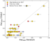 |
Fig. C.1. CIGALE-derived AGN fractions of this study, compared to the corresponding fractions calculated in previous works. Yellow circles, red squares, and filled blue ‘Xs’ depict the comparison with AGN fractions by Díaz-Santos et al. (2017), Fritz et al. (2006), and Ramos et al. (2020). All the data come with their error bars (black), while the grey solid line stands for the one-to-one relation. |
In Fig. C.2 we present the comparison of four basic parameters for the galaxies (namely, Mstar, Mdust, SFR, and Tdust) between the values derived in U et al. (2012) and the current work (with additional information from Casey 2012 and Herrero-Illana et al. 2019 for the case of Tdust).
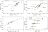 |
Fig. C.2. Comparison between the CIGALE derived properties (this work), Mstar (top-left panel), Mdust (top-right panel), the SFR (bottom-left panel), and Tdust (bottom-right panel) and the corresponding properties presented in U et al. (2012). Pink octagons indicate sources with strong AGN (fracAGN > 0.2). Wherever available, values come with their uncertainties. The grey solid line corresponds to the one-to-one relation. Extreme outliers are indicated with their IRAS names. In the bottom-right panel, green diamonds correspond to the comparison with the dust temperatures derived in Casey (2012), while blue boxes correspond to the comparison with the ones derived in Herrero-Illana et al. (2019). In this panel, sources with strong AGN are indicated by a pink edge-colour. |
In the top-left panel of Fig. C.2, we compare the stellar masses between the two studies. In U et al. (2012), two different IMFs were considered from Salpeter (1955) and Chabrier (2003). We compare them with the Salpeter IMF since this is the one considered in the current study. The stellar masses derived in U et al. (2012) were computed with two methods by performing an optical-NIR SED fitting, adopting the Bruzual & Charlot (2003) stellar population synthesis model, or by scaling from the H-band luminosity. Since the SED modelling method adopted in U et al. (2012) differs from the one used in the current work, we chose to compare our results with the scaling method for the H-band luminosity. The H-band, being largely unaffected by dust attenuation and also from contamination by hot dust emission from AGNs (Hainline et al. 2011) is a reliable tracer of the stellar mass. From Fig. C.2, we see an overall good agreement between the two studies (we find an average difference of 0.096 dex), with only a few exceptions substantially deviating from the one-to-one relation (the difference becomes 0.077 dex when the outliers are not considered). For F09333+4841, the JHK band fluxes reported in U et al. (2012) appear to be an order of a magnitude lower when compared to the optical and MIR fluxes. This makes the stellar mass calculated in U et al. (2012) underestimated. In the relevant SED presented in Fig. B.1, we re-scaled the JHK fluxes by an order of a magnitude higher, although this was not taken into account in the fit. F14547+2449, another outlier on this relation, appears as VV340a in U et al. (2012), indicating that only one member of this double system is treated (although not explicitly explained in the text). This could explain the lower stellar mass found in that study. Furthermore, the SED in their Fig. 2 appears twice, which makes it difficult to judge if their fit was successful or not. Finally, concerning F23488+2018, appearing as MRK0331 in U et al. (2012), we believe that their fitted SED (see their Fig. 2) might have overestimated the FUV fluxes, resulting in lower stellar mass. On the other hand, for F12224-0624, although the stellar masses are marginally consistent within the errors, it is also deviating from the one-to-one relation. Since this is a galaxy that accounts for the highest dust-to-stellar mass ratio (0.012), we believe that the differences are due to the significant effects of the dust on the stellar mass computation. In this plot, we also indicate the galaxies with the largest AGN fractions (fracAGN > 0.2; pink octagons). It is evident that the majority of the stronger AGNs in our sample are hosted in galaxies on the high-end of the stellar masses.
In the top-right panel of Fig. C.2, we present the comparison of the dust masses derived in U et al. (2012) and in our work. We find that, apart from some outliers, which are going to be discussed later, the derived masses between the two methods agree with a systematic offset of 0.46 dex (0.45 when the outliers are not considered). This can be explained by the use of the different dust absorption coefficients (κ850 = 0.15 m2 kg−1 and κ250 = 17.3 cm2 g−1; assuming an emissivity index of β = 2) in the case of U et al. (2012) compared to κ250 = 6.4 cm2 g−1 dictated by the THEMIS model (used in the current study), which translates to a 0.43 dex difference. Concerning the obvious outliers in this plot, we see that the majority of them host a luminous AGN (with fracAGN > 0.2; pink octagons) making the estimation of the dust mass quite uncertain if no AGN component is considered in the modelling. In the case of F04097+0525, we believe that in U et al. (2012), the dust is underestimated due to the fact that the Reyleigh-Jeans part of the SED is not well fitted (only constrained by the 850 μm observation); whereas in the current work, the Herschel data fill this gap and a more accurate determination of the dust mass is achieved. A similar case is F14348-1444 with the dust emission only being constrained by the IRAS 60 and 100 μm observation in the case of U et al. (2012), compared to our analysis where Herschel observations are also available.
In the bottom-left panel of Fig. C.2, we present the comparison of the SFR derived in U et al. (2012) and in our work. In U et al. (2012), the SFR is derived by combining the monochromatic UV luminosity at 2800 Å and the IR luminosity, using the Wuyts et al. (2011a) recipe. Since the IMFs used in the two methods are different, the values derived with the Chabrier IMF were divided by a constant scaling factor of 0.63 (Madau & Dickinson 2014). We see that there are some obvious outliers (with F13197-1627 being the most extreme case) though all are amongst the strongest AGNs in our sample with fracAGN > 0.2 (pink octagons). Since the IR luminosity may be largely affected by the presence of the AGN (see, e.g., the SED of F13197-1627), it is expected that the SFR is overestimated when the IR luminosity is used as an SFR tracer. The difference between the two methods is 0.12 dex (with 0.08 dex when the outliers are not considered).
In the bottom-right panel of Fig. C.2, the comparison among the values of Tdust derived in this work and the studies of U et al. (2012), Casey (2012), and Herrero-Illana et al. (2019; yellow circles, green diamonds, and blue boxes, respectively) is presented. The strongest AGNs in our sample (those with fracAGN > 0.2) are indicated in pink, while the line is the one-to-one relation. In all three literature studies mentioned above, the dust temperature was estimated by fitting a single temperature modified black-body to observations landwards of ∼70 μm. One thing to notice is that the resulting values of our study come in discrete ranges in dust temperature. This is due to the discrete nature of the parameter space used by CIGALE and, in particular, for the parameters that define Umin (see Eq. (1)). Even if the scatter is large, it is evident that the values derived in this work follow the general trend observed in other studies. The average difference and the standard deviation of the differences between our values and the literature values, which is −0.96 ± 4.3 K, are indicative of the scatter. As can be seen, though, from Fig. C.2, there are several outliers, the majority of them being AGNs (see the data points covered with pink colour). If these outliers are omitted from the statistics, the average difference and the standard deviation of the differences in dust temperature then drop to 0.09 ± 2.5 K. The most extreme example is F13197-1627 which shows the largest deviation. This is the strongest AGN in our sample (fracAGN = 0.85) with the AGN component occupying a large part of the FIR emission (see Fig. B.1) resulting in misleading results if a pure dust emission model is only fitted.
Appendix D: Cumulative distributions
Examining the cumulative distributions of the various physical parameters is a powerful tool that may indicate if two populations of objects can originate from the same parent population or not. The Kolmogorov-Smirnov Smirnov (1948) test is a well known non-parametric statistical method that compares distributions by measuring a ‘difference’ between the distributions and reports a p-value which shows a statistical significance of the result. A non-zero p-value of less than 0.15 means that the null hypothesis that the distributions come from the same parent distribution can be rejected with 85% probability (see, e.g., Haan et al. 2011).
In Fig. D.1, we present the cumulative distributions of the physical parameters presented in Sect. 4.2 (see also Fig. 4) for the three different populations of ETGs, LTGs, and (U)LIRGs (red, blue, and yellow colour, respectively). As can be seen from the plots, the relevant distributions are very different among the three galaxy populations with p-values less than 0.15. The only exception being the comparison of the temperature distributions between ETGs and LTGs, which give a p-value of 0.82. A relevant discussion on the results of the KS tests is presented in Sect. 4.2.
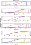 |
Fig. D.1. Cumulative distributions of the physical parameters discussed in this study for each galaxy type. The colouring is identical to Fig. 4. |
In Fig. D.2 the cumulative distributions of the physical parameters are presented in Sect. 5 (see also Figs. 6, 7, 8) for the different merging stages. The p-values drawn from the cumulative distributions of all the combinations of merging stages for each physical parameter are given in Table D.1. A relevant discussion on the results of the KS tests is presented in Sect. 5.
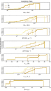 |
Fig. D.2. Cumulative distributions of the physical parameters discussed in this study for galaxies in merger stages ‘s’, ‘M1’, and ‘M3’. The colouring is identical to Fig. 6. |
Kolmogorov-Smirnov (KS) test p-values of the physical properties (Mdust, Mstar, SFR, sSFR, Tdust, LPDR, and fracAGN) for all the merging stage combinations. All p-values ≤0.15 are underlined.
All Tables
Mean values of the ratios of various combinations of the stellar and dust luminosity components extracted using the CIGALE SED fitting tool. These ratios are presented for the three general galaxy populations compared in this study (ETGs, LTGs, and (U)LIRGs), as well as for the seven merging classes of (U)LIRGs.
Kolmogorov-Smirnov (KS) test p-values of the physical properties (Mdust, Mstar, SFR, sSFR, Tdust, LPDR, and fracAGN) for all the merging stage combinations. All p-values ≤0.15 are underlined.
All Figures
|
Fig. 1. Distributions of the basic properties of our galaxy sample. The redshift distribution is plotted in the top-left panel and the number of sources per merging class is in the top-right panel. In the bottom-left panel, the IR luminosity distribution, based on IRAS observations (Sanders et al. 2003) is shown, while the bolometric AGN fractions calculated in Díaz-Santos et al. (2017) are plotted in the bottom-right panel. |
| In the text | |
|
Fig. 2. Template SEDs of the DustPedia ETGs (top-left panel), LTGs (top-right panel), and the local (U)LIRGs (bottom-left panel), as modelled by CIGALE. The black curves indicate the median SEDs, while the blue and red curves denote the median unattenuated SEDs of the young and old stellar populations, respectively. The median distribution of the diffuse dust is shown by the orange curve and the emission from the PDRs is shown by the green curve. The purple curve, in the bottom-left panel, indicates the median AGN distribution. The shaded areas cover the range between the 16th and 84th percentiles to the median values. For clarity reasons, since the PDR and the AGN components may vary substantially, we chose not to present the percentile widths of the curves. The median SEDs of the three different types of local galaxies are plotted in the bottom-right panel. The red curve represents the median, observed, SED of ETGs, the blue curve represents the one of LTGs, while the yellow curve corresponds to the median SED of (U)LIRGs. The thin, dotted curves show the unattenuated total stellar emission for the different classes. The reader is also referred to the corresponding median SEDs in Bianchi et al. (2018) and Nersesian et al. (2019). |
| In the text | |
|
Fig. 3. Correlations of SFR with stellar mass and dust mass (upper and middle panels respectively), and between fabs and Lbolo (bottom panel; see the text for the definition of the parameters). The DustPedia ETGs and LTGs are shown with red and blue circles, respectively, while yellow stars are the local (U)LIRGs in our sample. All values are plotted along with their corresponding uncertainties. In all plots, magenta dash-dotted, cyan dotted, and yellow dashed lines are the linear fits to the ETGs, LTGs, and (U)LIRGs, respectively. The black solid lines correspond to the best fits found in Elbaz et al. (2007) to the 0.015 ≤ z ≤ 0.1 SDSS star-forming galaxies (top panel), to the best fit found in da Cunha et al. (2010b) for a sample of low redshift galaxies (middle panel), and to the best fit found in Bianchi et al. (2018) for the DustPedia galaxies with T ≥ 2.5 (bottom panel). |
| In the text | |
|
Fig. 4. Physical properties, as derived by CIGALE, for the different galaxy types. From top to bottom, Mdust, Mstar, sSFR, Tdust, and LPDR are plotted as a function of galaxy type. Each red and blue dot corresponds to an individual ETG and LTG galaxy, while yellow dots correspond to (U)LIRGs, respectively. Black diamonds stand for the median values per galaxy type, while the associated 16th and 84th percentile ranges are indicated with error bars. Side plots of the distributions of each galaxy type for all the physical properties are also presented, following the same colouring as for the dots. In the bottom panel (LPDR), the median value of ETGs is dragged down to lower values because CIGALE predicts no PDR contribution for some sources (see the text for more details). |
| In the text | |
|
Fig. 5. Median SEDs of the local (U)LIRGs, separated in classes based on their merging stage. Classes ‘s’, ‘m’, and ‘M1’ are presented in the three top panels (from left to right), and classes ‘M2’, ‘M3, and ‘M4’ are presented in the three middle panels, while in the bottom-left panel the median SED of the ‘M5’ class is plotted. The curves and the shaded areas are coloured in the same manner as in Fig. 2. The bottom-right panel shows the comparison among the median SEDs of ‘s’, ‘M1’, and ‘M3’ classes, allowing for the differences to be spotted. |
| In the text | |
|
Fig. 6. SFR of (U)LIRGs in different merging stages, as derived from CIGALE. Each circle corresponds to an individual source. Black diamonds stand for the median values per merging class, while error bars indicate the range between the 16th and 84th percentiles from the median. Side plots of the distributions of class ‘s’, ‘M1’, and ‘M3’ systems, with the corresponding colour, are also presented. |
| In the text | |
|
Fig. 7. AGN fraction of (U)LIRGs in different merging stages, as derived from CIGALE, along with distributions for the class ‘s’, ‘M1’, and ‘M3’ systems. The style of markers is the same as in Fig. 6 |
| In the text | |
|
Fig. 8. Physical properties, as derived by CIGALE, for the seven different merging classes of (U)LIRGs. From top to the bottom, Mdust, Mstar, sSFR, Tdust, and LPDR are plotted as a function of the merging class. Each circle (following the colour coding of Fig. 6) corresponds to an individual system. Black diamonds stand for the median values per galaxy type, while the associated 16th and 84th percentile ranges are indicated with error bars. Distributions of class ‘s’, ‘M1’, and ‘M3’ systems, with the corresponding colour, are also presented as side plots. |
| In the text | |
|
Fig. 9. Comparison of the fraction of the young stellar population in seven systems in common between the sample studied here (YSPCIGALE) and the sample of Rodríguez Zaurín et al. (2009). In Rodríguez Zaurín et al. (2009), the young stellar populations (YSPspectra) were derived through spectral synthesis population modelling of optical long-slit spectra (see the text for more details). |
| In the text | |
|
Fig. 10. Left panel: contribution of the old (red) and young (blue) stellar populations to the unattenuated luminosity, over the bolometric luminosity, per galaxy type and (U)LIRGs merging class. Right panel: contribution of the old and young stellar populations to the attenuated luminosity, over the bolometric luminosity, per galaxy type and (U)LIRGs merging class (same colours as in left panel), together with the ratio of the dust luminosity to the bolometric luminosity (yellow). |
| In the text | |
|
Fig. 11. Mean values of the fraction of the luminosity of the old and the young stellar populations (left and right panel, respectively) used for the dust heating. The crossed bars show the mean values of the ratio of the dust-absorbed luminosity to the unattenuated luminosity of the corresponding stellar component, while the solid bars are the ratios of the attenuated luminosity of the specific stellar component to its unattenuated luminosity. In each panel, the ratios are presented for each of the three galaxy populations (ETGs, LTGs, and (U)LIRGs) in the leftmost sub-panel, and for the four merging classes in the rightmost sub-panel. |
| In the text | |
|
Fig. 12. Mean values of the ratios of the dust-absorbed stellar luminosity (originating from old and young stars) to the dust luminosity (red and blue colours, respectively). The ratios are presented for each of the three galaxy populations (ETGs, LTGs, and (U)LIRGs) in the leftmost sub-panel and for the four merging classes in the rightmost sub-panel. |
| In the text | |
|
Fig. A.1. Best fitted parameters (input values; x-axis) versus the mock parameters (mock values; y-axis) as derived by the mock analysis performed with CIGALE. Each circle corresponds to an individual galaxy with the red circles indicating the strongest AGNs in the sample with fracAGN > 0.2. The solid blue line corresponds to the one-to-one relation, while the orange dashed line corresponds to the best linear fit to the data. The relevant value of the Spearman’s correlation coefficient (ρ) is also indicated in each panel. |
| In the text | |
|
Fig. B.1. Best-fit SED models for the 67 galaxies in the current sample containing the unattenuated emission by the old (red) and the young (blue) stellar populations, the nebular line emission (dark-yellow), the diffuse dust (orange), the emission from the PDR regions (green), as well as the AGN emission (purple) are also presented. The best-fit SED is indicated as a black curve, while the observations for each galaxy, along with their uncertainties, are indicated by violet open squares. Light-green dots stand for the best-model flux densities. |
| In the text | |
|
Fig. B.1. continued. |
| In the text | |
|
Fig. B.1. continued. |
| In the text | |
|
Fig. B.1. continued. |
| In the text | |
|
Fig. B.1. continued. |
| In the text | |
|
Fig. B.1. continued. |
| In the text | |
|
Fig. B.1. continued. |
| In the text | |
|
Fig. B.1. continued. |
| In the text | |
|
Fig. B.1. continued. |
| In the text | |
|
Fig. C.1. CIGALE-derived AGN fractions of this study, compared to the corresponding fractions calculated in previous works. Yellow circles, red squares, and filled blue ‘Xs’ depict the comparison with AGN fractions by Díaz-Santos et al. (2017), Fritz et al. (2006), and Ramos et al. (2020). All the data come with their error bars (black), while the grey solid line stands for the one-to-one relation. |
| In the text | |
|
Fig. C.2. Comparison between the CIGALE derived properties (this work), Mstar (top-left panel), Mdust (top-right panel), the SFR (bottom-left panel), and Tdust (bottom-right panel) and the corresponding properties presented in U et al. (2012). Pink octagons indicate sources with strong AGN (fracAGN > 0.2). Wherever available, values come with their uncertainties. The grey solid line corresponds to the one-to-one relation. Extreme outliers are indicated with their IRAS names. In the bottom-right panel, green diamonds correspond to the comparison with the dust temperatures derived in Casey (2012), while blue boxes correspond to the comparison with the ones derived in Herrero-Illana et al. (2019). In this panel, sources with strong AGN are indicated by a pink edge-colour. |
| In the text | |
|
Fig. D.1. Cumulative distributions of the physical parameters discussed in this study for each galaxy type. The colouring is identical to Fig. 4. |
| In the text | |
|
Fig. D.2. Cumulative distributions of the physical parameters discussed in this study for galaxies in merger stages ‘s’, ‘M1’, and ‘M3’. The colouring is identical to Fig. 6. |
| In the text | |
Current usage metrics show cumulative count of Article Views (full-text article views including HTML views, PDF and ePub downloads, according to the available data) and Abstracts Views on Vision4Press platform.
Data correspond to usage on the plateform after 2015. The current usage metrics is available 48-96 hours after online publication and is updated daily on week days.
Initial download of the metrics may take a while.