| Issue |
A&A
Volume 647, March 2021
|
|
|---|---|---|
| Article Number | A145 | |
| Number of page(s) | 24 | |
| Section | Extragalactic astronomy | |
| DOI | https://doi.org/10.1051/0004-6361/202039644 | |
| Published online | 25 March 2021 | |
The Fornax3D project: Assembly histories of lenticular galaxies from a combined dynamical and population orbital analysis
1
Research Centre for Astronomy, Astrophysics, and Astrophotonics, Department of Physics and Astronomy, Macquarie University, Macquarie Park, NSW 2109, Australia
e-mail: adriano.poci@students.mq.edu.au
2
European Southern Observatory, Karl-Schwarzschild-Straße 2, 85748 Garching bei München, Germany
3
Shanghai Astronomical Observatory, Chinese Academy of Sciences, 80 Nandan Road, Shanghai 200030, PR China
4
Department of Astrophysics, University of Vienna, Türkenschanzstraße 17, 1180 Wien, Austria
5
INAF – Astronomical Observatory of Capodimonte, Salita Moiariello 16, 80131 Naples, Italy
6
Max-Planck-Institut für Astronomie, Königstuhl 17, 69117 Heidelberg, Germany
7
Dipartimento di Fisica e Astronomia ‘G. Galilei’, Università di Padova, Vicolo dell’Osservatorio 3, 35122 Padova, Italy
8
INAF – Osservatorio Astronomico di Padova, Vicolo dell’Osservatorio 5, 35122 Padova, Italy
9
Instituto de Astrofísica de Canarias, Calle Via Láctea s/n, 38200 La Laguna, Tenerife, Spain
10
Depto. Astrofísica, Universidad de La Laguna, Calle Astrofísico Francisco Sánchez s/n, 38206 La Laguna, Tenerife, Spain
11
Max-Planck-Institut für Astrophysik, Karl-Schwarzschild-Straße 1, 85748 Garching bei München, Germany
12
Armagh Observatory and Planetarium, College Hill, Armagh BT61 9DG, UK
13
Centre for Astrophysics Research, University of Hertfordshire, College Lane, Hatfield AL10 9AB, UK
14
Sterrenkundig Observatorium, Universiteit Gent, Krijgslaan 281, 9000 Gent, Belgium
15
Sterrewacht Leiden, Leiden University, Postbus 9513, 2300 RA Leiden, The Netherlands
16
Max-Planck-Institut für Extraterrestrische Physik, Gießenbachstraße 1, 85748 Garching bei München, Germany
Received:
11
October
2020
Accepted:
1
February
2021
In order to assess the impact of the environment on the formation and evolution of galaxies, accurate assembly histories of such galaxies are needed. However, these measurements are observationally difficult owing to the diversity of formation paths that lead to the same present-day state of a galaxy. In this work, we apply a powerful new technique in order to observationally derive accurate assembly histories through a self-consistent combined stellar dynamical and population galaxy model. We present this approach for three edge-on lenticular galaxies from the Fornax3D project – FCC 153, FCC 170, and FCC 177 – in order to infer their mass assembly histories individually and in the context of the Fornax cluster. The method was tested on mock data from simulations to quantify its reliability. We find that the galaxies studied here have all been able to form dynamically-cold (intrinsic vertical velocity dispersion σz ≲ 50 km s−1) stellar disks after cluster infall. Moreover, the pre-existing (old) high angular momentum components have retained their angular momentum (orbital circularity λz > 0.8) through to the present day. Comparing the derived assembly histories with a comparable galaxy in a low-density environment – NGC 3115 – we find evidence for cluster-driven suppression of stellar accretion and merging. We measured the intrinsic stellar age–velocity-dispersion relation and find that the shape of the relation is consistent with galaxies in the literature across redshift. There is tentative evidence for enhancement in the luminosity-weighted intrinsic vertical velocity dispersion due to the cluster environment. But importantly, there is an indication that metallicity may be a key driver of this relation. We finally speculate that the cluster environment is responsible for the S0 morphology of these galaxies via the gradual external perturbations, or ‘harassment’, generated within the cluster.
Key words: galaxies: kinematics and dynamics / galaxies: stellar content / galaxies: structure / galaxies: formation / galaxies: elliptical and lenticular, cD / galaxies: evolution
© ESO 2021
1. Introduction
Galaxy formation and evolution is the culmination of competing forces and processes over each galaxy’s lifetime. These processes can be internal to the galaxy, such as the energy generated by the central super-massive black hole (SMBH) or the winds generated by star formation. They can also have external origins, such as the gravitational potential of other galaxies (Toomre & Toomre 1972) or cosmic gas filaments. Due to this ‘superposition’ of evolutionary processes, it is difficult to isolate the impact on the galaxy from only one of them, especially when many are still occurring. The environment which a galaxy inhabits has long been suspected of altering its evolutionary path (Gunn & Gott 1972; Dressler 1980; Postman & Geller 1984; Ryden et al. 1993), but with conflicting results on the exact impact. Field environments are relatively simple and provide a control sample for comparison with higher-density environments such as groups and clusters. This comparison is not straight forward, however, since cluster environments are a complex mixture of many, often dramatic, physical processes such as gravitational disruption (owing to the significantly deeper gravitational potential), hydrodynamic effects due to the hot intra-cluster medium (ICM), and thermodynamic effects such as shocks due to the high relative velocities that a galaxy can experience when it first encounters the ICM during in-fall.
A number of correlations have been observed between galactic observables and some metric for the local environment. Historically, the projected density of galaxies or Nth nearest neighbour measurements of the local density have been found to correlate with visual morphology (e.g., Dressler 1980; Cappellari et al. 2011a; Oh et al. 2018; Gargiulo et al. 2019) and invoked to explain morphological transformations (e.g., Bekki et al. 2002; Kauffmann et al. 2004; Blanton et al. 2005; D’Onofrio et al. 2015; Coccato et al. 2020). Yet morphology has also been observed to correlate with stellar mass at fixed local density (van der Wel 2008), and so the underlying cause is difficult to discern. This problem permeates through most observed correlations. Some works have shown that galaxies exhibit a lower net angular momentum for a higher local density (e.g., Cappellari et al. 2011b; Cortese et al. 2019; Graham et al. 2019; Cole et al. 2020), while others find that there is no additional dependence on the environment once the correlation between the angular momentum and stellar mass is accounted for (Brough et al. 2017). Finally, the stellar population parameters also suffer from conflicting correlations. Some observations indicate reduced star-formation activity (e.g., Balogh et al. 2004; Poggianti et al. 2006; Allen et al. 2016; Owers et al. 2019), a higher stellar metallicity (e.g., Schaefer et al. 2019), older stellar ages (e.g., Thomas et al. 2005; McDermid et al. 2015), and a lower gas content (e.g., Zabel et al. 2019) for higher local density, while others indicate that stellar mass is the driver instead of environment (Alpaslan et al. 2015; Goddard et al. 2017). Many of these correlations have also been found in recent cosmological hydrodynamical simulations (e.g., Choi et al. 2018; Wang et al. 2018a,b). More broadly, it is not straight forward to disentangle the effects of mass and environment, and it is likely that both play a role (Peng et al. 2010; Smith et al. 2012; McDermid et al. 2015; Wang et al. 2020), and joint analyses over all available parameters are needed such as those applied by Christlein & Zabludoff (2005) to global galaxy properties. The morphology, mass, and other galactic properties are intricately connected through each galaxy’s unique assembly history. It is therefore clear that to uncover what impact the environment has, if any, the complete assembly history must be investigated directly as a function of the environment.
The dynamical memory of galaxies plays an important role in attempting to disentangle such assembly histories, assisted by the (often long) dynamical times of galactic systems. As such, the stellar kinematics can provide insight into this history. Dynamical models of stellar kinematics have been employed to measure constraints on galaxy formation for a variety of morphological types and environments, based on a number of different principles. The Jeans equations have been readily applied owing to their relative simplicity and computational efficiency (e.g., Cappellari et al. 2013; Watkins et al. 2013; Zhu et al. 2016a,b; Poci et al. 2017; Bellstedt et al. 2018; Nguyen et al. 2019; Nitschai et al. 2020; Li et al. 2020; Cappellari 2016 for a review), though with specific assumptions about the intrinsic velocity distributions of galaxies. Distribution-function models (e.g., Cole & Binney 2017; Taranu et al. 2017; Pascale et al. 2018) can be quite general and computationally-efficient, but usually use parametric expressions which may not provide enough freedom. Finally, the Schwarzschild (1979) orbit-superposition method provides a general approach without the assumption of specific distribution functions or density distributions, while also providing a wealth of information on the intrinsic properties of the model. Though it is far more computationally-expensive, it has seen a growing diversity of applications (e.g., van der Marel et al. 1998; Cretton et al. 1999; Verolme & de Zeeuw 2002; Gebhardt et al. 2003; Valluri et al. 2004; Cappellari et al. 2006; Krajnović et al. 2009, 2015; Vasiliev 2013, 2019; Leung et al. 2018; Zhu et al. 2018a,b; Vasiliev & Valluri 2020). Through these models, a galaxy’s merger history can be traced through the potentially-complex observed kinematics, but only when confronted with a sufficiently-sophisticated dynamical model which can access the underlying intrinsic properties (e.g., van den Bosch et al. 2008; Lyubenova et al. 2013; Krajnović et al. 2015). However, purely-dynamical models can not produce a chronological assembly history, since they lack information about the ages of the stars and where they might have originated.
This work is part of the Fornax3D survey; an observational programme to study the Fornax galaxy cluster with the Multi-Unit Spectroscopic Explorer (MUSE) at VLT. In total, the survey observed 31 members of the Fornax cluster with mB < 15 mag, at or interior to the Virial radius (Rvir ∼ 0.7 Mpc; Drinkwater et al. 2001). Fornax is a well-surveyed (Drinkwater et al. 2001; Jordán et al. 2007; Davies et al. 2013; Muñoz et al. 2015; Iodice et al. 2016; Pota et al. 2018; Sarzi et al. 2018; Zabel et al. 2019; Scott et al. 2020) galaxy cluster at a distance D ∼ 20 Mpc, and with a total halo mass of log10(Mhalo/M⊙) ∼ 13.85 (Jordán et al. 2007). The application of the Schwarzschild models to Fornax3D data was showcased in Sarzi et al. (2018), and a qualitative comparison to the stellar populations was made in Martín-Navarro et al. (2019). In this work, we aim to measure complete chronological assembly histories of three edge-on S0 galaxies – FCC 153, FCC 170, and FCC 177 – by quantitatively combining these sophisticated dynamical modelling techniques with the measured stellar populations. They are discussed in conjunction with a previous application of this method (Poci et al. 2019) to a massive [log10(M⋆/M⊙) ∼ 11] field S0, NGC 3115, to probe any potential impact of the cluster environment.
This work is organised as follows: the data and target selection are briefly outlined in Sect. 2, and the combined dynamical and population modelling is detailed in Sect. 3. Results for each galaxy are presented in Sect. 4. The implications of these results in the context of the Fornax cluster and specific quantitative correlations are investigated in Sect. 5.
2. Data and targets
2.1. Photometry
The photometric data for this work is taken from the Fornax Deep Survey (FDS; Iodice et al. 2016; Venhola et al. 2018), which acquired deep photometry of the Fornax cluster out to in the u, g, r, and i bands using the Very Large Telescope (VLT) Survey Telescope (VST). We utilise the r-band photometry to model the surface brightness distribution of these galaxies. We also make use of the g−i colour to characterise the mass distribution beyond the field-of-view (FOV) of the spectroscopy (see Sect. 3.1). FDS data extend down to a surface brightness of μr ∼ 28 mag arcsec−2 in the r band.
Distances to these galaxies were measured in Blakeslee et al. (2009) via surface-brightness fluctuations. We adopt those measurements here, given in Table 1.
Physical properties of the galaxy sample.
2.2. Spectroscopy
The spectral data are taken from the Fornax3D project (Sarzi et al. 2018). In this work, all data products are computed on the spectral range λ ∈ [4600, 6700] Å. This range avoids the problematic sky emission lines and telluric effects. It is wide enough, however, to include many of the important absorption features for the stellar population analyses. Moreover it encapsulates the bandwidth of the r filter of VST which is utilised in conjunction with the spectroscopy to describe the luminosity density of the stellar kinematic tracer. To prepare the data products, the data-cubes are spatially binned to a target signal-to-noise ratio (S/N) of 100 using the Python implementation1 of the Voronoi binning technique (Cappellari & Copin 2003). This ensures that the kinematic and stellar-population measurements can achieve measurement errors ≲ 5% (shown in Appendix B).
Kinematics are extracted for each binned spectrum using the pPXF (Cappellari & Emsellem 2004; Cappellari 2017) Python package2, which determines the line-of-sight velocity distribution (LOSVD) through moments of the Gauss-Hermite series. We extract the first six moments of the LOSVD in each bin; mean velocity V, velocity dispersion σ, skewness h3, kurtosis h4, and higher-order deviations h5 and h6. pPXF is run with the MILES empirical stellar library (Falcón-Barroso et al. 2011), and with an additive polynomial of degree 10 in order to accurately reproduce the line shapes. Naturally, spectra are dominated by the brightest components of the observed galaxies through the LOS, and so the extracted kinematics are effectively luminosity-weighted.
Star formation histories (SFH) and their mean stellar population properties are extracted by running pPXF with the E-MILES single stellar population (SSP) templates (Vazdekis et al. 2016) using the ‘BaSTI’ isochrone models (Pietrinferni et al. 2004). A multiplicative polynomial of degree 10 is included in order to account for the continuum without affecting the relative line shapes. The SSP models are normalised such that we measure luminosity-weighted stellar populations, in order to maintain consistency with the stellar kinematics and subsequent dynamical model (described in Sect. 3.2). The stellar-population fits use a first-derivative linear regularisation with Δ = 1.0, which prefers a smoother solution in the case of degeneracy between the SSP models. We assume a fixed Kroupa (2002) galaxy initial mass function (IMF). The canonical Salpeter (1955) IMF has been shown to disagree with the mass-to-light ratios from stellar dynamics (Lyubenova et al. 2016), while the low central velocity dispersion of these galaxies (Iodice et al. 2019a) is consistent with an IMF which is relatively deficient of dwarf stars (e.g., Thomas et al. 2011; Cappellari et al. 2012; Wegner et al. 2012). In this work, we explore the projected distribution of mean stellar age (t) and metallicity (total metal abundance, [Z/H]). Representative spectral fits are presented in Fig. 1.
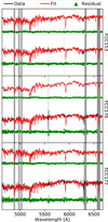 |
Fig. 1. Fits (red) to spectra (black) from the centre and outer regions (top and bottom of each pair of spectra, respectively) for our galaxy sample, as labelled on the right. Residuals are shown in green, offset for presentation. The grey bands show regions which are masked during the fit. All spectra are normalised, but vertically offset for presentation. It can be seen that the outer spectra are more noisy, as expected, but that in all cases the data are reproduced well by the fit. |
The solutions from the stellar-population run of pPXF and the predictions from E-MILES (Vazdekis et al. 2010) then enable the derivation of the r-band stellar mass-to-light ratio (M⋆/LR) for each spectrum, using the mass in stars and stellar remnants for the assumed IMF. This is utilised for the dynamical modelling (Sect. 3.1). We generate Monte Carlo fits to the spectra by adding random noise within the variance spectra in the data-cubes. Each spectrum is re-fit 100 times to generate a new distribution of SSP weights. Luminosity-weighted properties are re-derived for each weight distribution. The ‘uncertainty’ in a given aperture is then estimated from the variance of luminosity-weighted properties across all Monte Carlo simulations in that aperture. These uncertainty maps (shown in Appendix B) are utilised to gauge the stability of our final results.
Similar data products have already been measured for these galaxies as part of Fornax3D (Pinna et al. 2019a,b; Iodice et al. 2019a). The motivation for re-extracting them in this work is to achieve higher S/N for higher-precision stellar population parameters (see, for instance, Asa’d & Goudfrooij 2020) and to minimise the impact of measuring σlos ≲ σinst (for the line-of-sight velocity dispersion and instrumental velocity resolution σlos and σinst, respectively; Cappellari 2017), albeit on larger spatial bins. Moreover, we fit the specific wavelength range, as discussed above. Finally, luminosity-weighted stellar populations are required for the analyses in this work as described above, while previous measurements are mass-weighted (Pinna et al. 2019a,b). The new kinematics from this work are consistent with previous measurements. The luminosity-weighted ages are systematically younger than the mass-weighted determinations while the metallicities are consistent, as expected (Serra & Trager 2007; McDermid et al. 2015).
2.3. Targets
For this work, due to the nature of our dynamical and population orbital analysis (Sect. 3), we selected a sub-sample of three galaxies: FCC 153, FCC 170, and FCC 177. These galaxies are all approximately edge-on, and have S0 morphology. They are suitable targets for our analysis because they show no signs of dust or spiral arms. This is important because the dynamical model assumes a steady-state gravitational potential while spiral arms are transient, and dust would impact the inferences of the stellar populations. Additionally, our methodology (Sect. 3) is most robust for edge-on systems. Each galaxy has a central and outer pointing from the Fornax3D survey, ensuring that the vast majority of the stellar body is covered while retaining the high spatial resolution of MUSE. The FDS r-band images of the three galaxies are shown in Fig. 2, with the MUSE outline shown in dashed brown. As measured from the FDS data, FCC 153, FCC 170, and FCC 177 are at a projected distance of 1.17°, 0.42°, and 0.79° from the cluster core, respectively (Iodice et al. 2019b). These galaxies have integrated g−i colours of 0.77 ± 0.07, 1.07 ± 0.02, and 1.80 ± 0.03, and r-band surface-brightness radial profiles which extend down to 28.9, 29.2, and 29.5 mag arcsec−2, respectively, as derived from the FDS photometry (Iodice et al. 2019b).
 |
Fig. 2. Full r-band images from FDS, overlaid with the MUSE FOV in dashed brown for FCC 153 (left), FCC 170 (middle), and FCC 177 (right). |
These galaxies are the focus of the spectral analyses presented in Pinna et al. (2019a,b), where their SFH are discussed in the context of the Fornax cluster. Those works conclude that FCC 170 matured more rapidly, having plausibly evolved in an earlier group environment in the initial stages of the Fornax cluster assembly. Conversely, FCC 153 and FCC 177 are seen to exhibit relatively smooth SFH in their thin disk regions. In the study on stellar accretion fractions in members of the Fornax cluster, Spavone et al. (2020) find that it is difficult to photometrically disentangle the various components of these three galaxies, since they have indistinguishable surface brightness profiles. They find that low accretion fractions (≲ 50%) are typical for other galaxies at cluster-centric radii similar to FCC 153 and FCC 177. Conversely, for galaxies in the region close to FCC 170, higher accretion fractions (≳ 50%) are derived. We aim, as part of this work, to place constraints on this fraction even for the galaxies which are photometrically degenerate.
3. Stellar content of galaxies
We endeavour to consider the complete stellar information content available through observations. The model we fit to these data was the self-consistent combination of Schwarzschild orbit-superposition dynamical models, using a triaxial implementation (van de Ven et al. 2008; van den Bosch et al. 2008), and stellar-population measurements derived from full spectral fitting. We employed the method described in Poci et al. (2019) for this combination. We therefore refer to that work and references therein for details, but lay out the basic structure of the method and the differences with that work in this section.
We also ensured that our data are tracing the galaxies themselves, and not components of the cluster environment. The FDS data show that FCC 170 is within the large-scale intra-cluster light (ICL) detected towards the cluster centre (Iodice et al. 2019a). This ICL component was measured to have total integrated magnitudes of 1.21 ± 0.3 and 11.4 ± 0.3 in g- and r-band, respectively, over an area of ∼ 432 arcmin2 (assuming a uniform surface brightness distribution; Iodice et al. 2017). At the distance and direction from the cluster centre to FCC 170, the ICL has a r-band surface brightness of ∼ 27.5 mag arcsec−2 (Iodice et al. 2017). In contrast, the spectroscopic data from the Fornax3D survey have a r-band target depth of 25 mag arcsec−2 in the faintest regions covered by the FOV. For our sample, the FOV extend to 4.90, 5.63, and 9.61 kpc along the major axis for FCC 153, FCC 170, and FCC 177, respectively, at our adopted distances (see Table 1). In all three cases, therefore, we expect the impact of the ICL on the measured properties to be negligible, being at least ∼ 100 times fainter than the faintest regions of the galaxies within our spectroscopic FOV.
3.1. Stellar mass model
One of the most crucial aspects of a dynamical model of stellar kinematics is the input mass model in which the observed tracer population resides. This is often derived from the observed photometry. We begin by fitting a multi-Gaussian Expansion (MGE; Monnet et al. 1992; Emsellem et al. 1994) to the r-band photometry from FDS using a Python implementation3 (Cappellari 2002). This produces a projected surface-brightness model (MGEμ), which serves as the luminous tracer of the gravitational potential of the galaxy. These models are shown in Appendix A.
To reconstruct the mass, the surface brightness must be converted into surface mass density. While standard implementations of Schwarzschild (and indeed dynamical) models assume a spatially-constant conversion from luminosity to mass, we exploit the spatially-resolved map of stellar M⋆/LR in order to account for the prominent structures and variations in the stellar populations that are resolved by the high-quality spectroscopy. We make additional use of the deep FDS photometry to constrain the stellar populations outside of the spectroscopic FOV to constrain the dynamical model well beyond the measured kinematics. We use the predictions from the E-MILES SSP models to derive a relation between g−i colours and M⋆/LR, which we assume to be of the form log10(M⋆/LR) ∝ (g − i) as found empirically (Tortora et al. 2011; Wilkins et al. 2013; McGaugh & Schombert 2014; Du & McGaugh 2020). The smaller spectroscopic FOV, which is used where available, is thus augmented by the larger photometric FOV to generate M⋆/LR on the same extent as the photometry. While the spectroscopic measurements of M⋆/LR reach ≲ 60″ for the three galaxies, the depth of the FDS survey allows this coverage to be extended to ∼ 150″ providing a dramatic improvement to the constraints of the mass model. Using this large-scale combined (spectroscopic and photometric) M⋆/LR map, MGEμ is then converted to a map of surface mass density, to which a mass density MGE (MGE∑) is fit. The fits and results for all MGE∑ are given in Appendix A. Figures A.1–A.3 show deviations of up to ± 30% compared to a spatially-constant M⋆/LR (in projection). This approach takes into account not just these deviations in the absolute scale, but also the structures of the stellar populations, producing a more accurate mass model and subsequent dynamical model.
The photometric measurements of M⋆/LR are effectively ‘SSP-equivalent’, while the spectroscopic values are derived from the full SFH. To mitigate any systematic offsets this may cause, the photometrically-derived values are re-scaled to match the spectroscopic values in the overlapping regions. We emphasise that the rapidly-varying spatial structures in the stellar populations – caused primarily by the thin edge-on disks – are captured by the spectroscopy, while the photometry is utilised only in the region where variations are mild. Coupled with the intrinsic symmetry of the MGE fitting, the photometric M⋆/LR serves to extend the range of the MGE model and stabilise the shape of the gravitational potential in that region. It can be seen in Figs. A.1–A.3 that there are no systematic offsets at the transition from spectroscopically- to photometrically-derived M⋆/LR, and the level of noise in the colour region is no greater than the pixel-to-pixel scatter in images to which MGE is typically applied. Overall, this procedure allows for the stellar populations to be more robustly accounted for.
3.2. Schwarzschild dynamical models
The basic premise of the Schwarzschild method is to numerically integrate a large number of permitted orbits within a model for the gravitational potential, then measure their kinematics and compare to observations. For real observations, the gravitational potential is of course unknown and must be iteratively fit for. To achieve this, we used a triaxial implementation of the Schwarzschild method that has been robustly developed and validated (van den Bosch et al. 2008; van de Ven et al. 2008; Zhu et al. 2018a,b, 2020; Jin et al. 2019). In this implementation, a single model is described by seven parameters:
-
(a)
the three parameters describing the intrinsic shape and viewing direction of the stellar mass distribution, q = C/A, p = B/A, and u = A′/A, where A, B, and C are the intrinsic major, intermediate, and minor axes, respectively, and A′ is the projected major axis.
-
(b)
the mass of the central SMBH, M∙.
-
(c)
the parameters of the dark matter (DM) profile, which is implemented as a spherical Navarro-Frenk-White (NFW) model (Navarro et al. 1996). These are the concentration CDM and dark mass fraction at r200, fDM.
-
(d)
a global dynamical mass-to-light ratio, which we denote Υ. This parameter can shift the global depth of the potential in order to better match the observed kinematics, but does not change its shape nor therefore which orbital families can reside within it. Υ is included to account for any deviations in the absolute depth of the gravitational potential due to the assumption of the IMF when computing the M⋆/L and/or systematics in the assumed DM halo model.
We streamlined the search through this large parameter-space by making reasonable assumptions about some of these parameters. The masses of the SMBH were fixed according to the empirical M∙ − σe relation of Kormendy & Ho (2013), using the σe measurements for these galaxies reported in Iodice et al. (2019a). In addition, we estimated the sphere of influence ri of each SMBH, which is utilised by the model but is not a free parameter, using the relation of van den Bosch et al. (2015). This is expected to have little impact on the model however – for the galaxy with the largest central velocity dispersion, FCC 170, ri ≈ 0.08″, which is below the pixel scale of MUSE. In addition, the stellar shape parameter u was fixed to u = (1.0 − ϵ) for some small number ϵ to avoid numerical issues. This assumption is reasonable since regular fast-rotator galaxies are found to be consistent with oblate intrinsic shapes (Weijmans et al. 2014). We note that mild triaxiality is still permitted in these models, with the condition that the potential must be axisymmetric in projection. The parameter-space is thus reduced to five dimensions; q, p, CDM, fDM, Υ.
Each Schwarzschild model corresponds to a unique intrinsic gravitational potential. The orbital families which can reside within each gravitational potential are therefore also unique. Thus, each location in the hyper-parameter-space is accompanied by its own library of numerically-integrated orbits. These orbits are characterised by the integrals of motion which they conserve, namely the binding energy E, angular momentum I2, and the third non-classical conserved integral I3. Each library of orbits was generated by sampling these integrals in (E, I2, I3) = (30, 20, 10) steps (logarithmically for E and linearly for I2 and I3; see Cretton et al. 2000, for details of the integral sampling). The region around the best-fit model was re-computed with a higher orbit sampling of (E, I2, I3) = (60, 30, 15) to increase the resolution of the resulting intrinsic properties. To avoid discreteness in these libraries, each orbit was dithered by a factor of 5, creating a cloud of orbits around each (E, I2, I3). Using a Non-Negative Least-Squares (NNLS; Lawson & Hanson 1995) fit, the model selects the best sub-set of orbits from each library which reproduces the observed kinematics in projection. It simultaneously fits a boundary constraint, which in this work is the projected luminosity distribution, such that the weights assigned to the orbits during NNLS are luminosity weights. Thus, each unique gravitational potential has a corresponding unique set of best-fit orbits.
By construction, Υ does not change the shape of the gravitational potential. In a gravitational potential with a fixed shape but varying Υ, the families of orbits do not change. Rather, the velocities of these orbits are simply scaled up or down to reflect a deeper or more shallow potential, respectively, and the NNLS fit is repeated for the scaled orbits. Therefore only four parameters require the computationally-expensive numerical integration of an orbit library. The five free parameters were optimised using an adaptive grid search, whose direction and step-size depend on the existing set of evaluated models, with a large initial spread to avoid local minima. The search terminated once all surrounding models were worse fits to the data. The kinematic fits are shown in the top seven rows of Figs. 7–9. The parameter-space searches and best-fit parameters are presented in Appendix B.
To avoid artificial bias in the model due to systematic asymmetries in the data, the even (odd) kinematic moments were point-(anti)symmetrised to be consistent with the intrinsic model symmetry4. These asymmetries present deviations of up to ∼ 6 km s−1 in velocity and velocity dispersion with respect to the symmetrised kinematics, which is of order the measurement uncertainties on the kinematics. The ‘raw’ un-symmetrised kinematics and their Monte Carlo-derived errors are shown in Appendix B.
The Schwarzschild models allow us to investigate the distribution of mass within these galaxies. Enclosed mass profiles are presented in Fig. 3, where the maximum extent of the spectroscopy is marked by Rmax, while useful quantities are provided in Table 1. It can be seen that FCC 170 is baryon-dominated within the spectroscopic FOV, while FCC 153 and FCC 177 transition to DM-dominated at or below their effective radii (given in Table 1). We also define Renc, the spherical radius which encloses 98% of the stellar mass (derived by integrating the stellar mass profile). This reduces the dependence of the mass profile on the lowest surface-brightness (most uncertain) regions. These radii are in good quantitative agreement with the maximum extent of the surface brightness profiles of Spavone et al. (2020). The corresponding stellar and DM masses within Renc are denoted by  and
and  , respectively. These are given in Table 1. The amount of stellar mass outside of the spectroscopic FOV can be estimated as log10[M⋆(R = Rmax)/M⋆(R = Renc). This gives 0.12, 0.09, and 0.07 dex, for FCC 153, FCC 170, and FCC 177, respectively. While the mass in this region (Rmax < R < Renc) is not directly constrained by the kinematics, it is still constrained by the mass model described in Sect. 3.1. We explore these mass distributions further in the sections below.
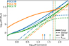 |
Fig. 3. Enclosed-mass profiles of the total (dynamical) mass (solid line), stellar mass (dashed line), and DM (dot-dashed line) for the three galaxies. The effective radii are denoted by the small arrows, and the radial extent of each spectroscopic FOV is shown by the vertical dotted line. The lower radial bound of the figure is set to half the width of the point-spread function from the spectroscopic observations. |
3.3. Dynamical decomposition
From the best-fit dynamical model, we used the phase-space of circularity (Zhu et al. 2018b), λz, and cylindrical radius, R, in order to conduct a dynamical decomposition. This radius represents the time-averaged cylindrical radius of each orbit over its orbital period. The circularity is a normalised measure of the intrinsic orbital angular momentum, and we used it here to divide the Schwarzschild model into orbits with varying degree of rotation (|λz| ∼ 1) or pressure (λz ∼ 0) support. In order to account for the structure in the kinematics and stellar-population maps simultaneously, and motivated by tests conducted in Poci et al. (2019), we divided the phase-space into many (∼ 102) ‘components’. This was achieved by imposing a log-linear grid on the circularity phase-space. The radial axis was sampled logarithmically, but with a floor on the grid size. This preserves the orbital sampling from the Schwarzschild model5 but avoids generating cells in the circularity phase-space which are below the spatial resolution of the data. The circularity axis was sampled linearly. This phase-space and corresponding dynamical decompositions are presented in Figs. 4–6 for FCC 153, FCC 170, and FCC 177, respectively. This sampling in λz − R was used for all three galaxies, however the final distribution of ‘components’ depends on the circularity distribution of each galaxy’s best-fitting Schwarzschild model.
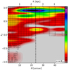 |
Fig. 4. Phase-space of circularity λz as a function of cylindrical radius R for the best-fit model of FCC 153. The colour represents the orbital weight from the Schwarzschild model, which has been normalised to an integral of unity. The dynamical decomposition is overlaid in black, where only those components which have non-zero contribution to the original model are defined. The figure is shown on the radial extent of the spectroscopy for clarity, but the decomposition is conducted over the full Schwarzschild model. The black dashed line is the half-mass radius, derived from MGE∑, shown for scale. The distribution indicates the prevalence of high-angular-momentum (cold disk-like) co-rotating orbits in this galaxy, with very little contribution from hot (λz ∼ 0) or counter-rotating (λz < 0) orbits. |
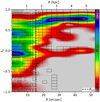 |
Fig. 5. Same as Fig. 4, but for FCC 170. This galaxy has a large contribution from hot central orbits, with most of the cold orbits appearing at larger radius. |
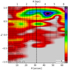 |
Fig. 6. Same as Fig. 4, but for FCC 177. Similarly to FCC 153, this galaxy is dominated by co-rotating cold orbits. |
A single component is composed of a unique subset of the orbit library of its parent Schwarzschild model. The decomposition is an effective way of simply bundling orbits of similar properties – in this case, angular momentum and radius. Kinematics, masses, and mass densities are computed for each component individually, based on its specific subset of orbits and those orbits’ relative contribution to the original dynamical model. Thus, each component has fixed projected kinematics and spatial distributions.
3.4. Adding stellar populations
We now describe the extension beyond the standard Schwarzschild approach for the inclusion of the stellar population measurements. In order to self-consistently combine the kinematics and stellar populations, we exploited the fact that both the derivation of the SFH from full spectral fitting and the construction of the Schwarzschild model are based on the same principle; they are weighted integrations over many distinct populations, integrated through the line-of-sight (LOS). Specifically, the measured stellar populations are luminosity-weighted by construction as described in Sect. 2.2, and the orbital weights are constrained by the surface brightness even though their dynamical properties are computed in the total gravitational potential. Therefore, we assume that the distributions of stellar and dynamical populations are the same. The weight distributions from the dynamical models were then used to derive the distributions of stellar populations that reproduce their observed maps. The result is that each orbit which contributes to the dynamical model now has an associated age and metallicity. Each dynamical component can thus be considered a mono-abundance population. By fitting age and metallicity independently, we avoided the possibility of degeneracies between them, as well as having to assume a specific age-metallicity relation. Instead, regularisation was utilised for each stellar-population fit, and is analogous to what is routinely used for spectral-fitting analyses such as in Sect. 2.2. The specific implementation is detailed in Poci et al. (2019). We tested this approach using mock data from the Auriga simulations (Grand et al. 2016), presented in Appendix C, and find that the main results of this work are accurate to ≲ 10% (Fig. C.4). An alternative approach which uses a chemical-evolution model to derive the age-metallicity relation is presented in Zhu et al. (2020).
The subsequent integration through the LOS of the stellar orbits reproduces all measured kinematic and stellar-population maps. Fits to all maps are shown in Figs. 7–9. We also conducted Monte Carlo simulations by re-fitting the stellar-population maps 100 times after randomly perturbing them within their measurement errors. These fits re-distribute the dynamical components in the t − [Z/H] plane (without changing their kinematics), and so were used to estimate the uncertainties of our results. Using all available information – kinematics, ages, metallicities, and density distributions – we can now investigate the formation events that built up each galaxy.
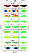 |
Fig. 7. Best-fitting Schwarzschild model for FCC 153. The data (left), fits (middle), and residuals (right) of, from top to bottom, the dynamical model (surface brightness, velocity, velocity dispersion, and h3 − h6), and the subsequent stellar-population fitting (age and metallicity). The outline of the MUSE mosaic is shown in dashed brown. All residual panels show the absolute differences (data – model), but are offset such that green is zero. The stellar-population maps share a common colour-bar between galaxies for comparison. We note that for FCC 153, since the observed metallicity map reaches 0.4 dex along the major axis, and is itself an average through the LOS, we extend the upper bound for the individual components during the stellar-population fitting to 1.0 dex. |
4. Combined dynamical and stellar populations
The combination of dynamical and stellar populations is imperative to be able to decode the integrated assembly history into its constituent events. We do this using the diagnostic power of Figs. 10–12 for FCC 153, FCC 170, and FCC 177, respectively. These figures show radial profiles of the intrinsic vertical stellar velocity dispersion σz(R) and the projected surface brightness distributions for each galaxy as a function of both age and metallicity. This combination of kinematic and population constraints effectively produces star-formation and accretion histories simultaneously, resulting in genuine mass assembly histories. The vertical velocity dispersion is a useful metric for discriminating between different dynamical structures, as well as being comparable to a variety of different observations (explored below). However, for dissecting the model into different dynamical regimes, we used the intrinsic orbital circularity to determine dynamical temperature as this property is inherently connected to the intrinsic orbital phase-space. Before exploring each galaxy individually, we first qualitatively discuss how various features of these figures are interpreted.
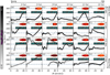 |
Fig. 10. Mass assembly history for FCC 153. The panels are ordered by increasing mean stellar age (left to right) and decreasing mean stellar metallicity (top to bottom). The value given at the top and right of each column and row, respectively, denotes its upper bound (inclusive). Each panel is composed of a radial profile of the vertical stellar velocity dispersion σz (black/white curve), the surface brightness distribution at the best-fitting projection (top-right) with the outline of the MUSE mosaic shown in dashed brown, and the total stellar mass within the FOV for that panel. The σz(R) profiles are coloured according to the stellar mass in that panel at that radius (sampled within the logarithmic radial bins). This indicates the spatial region in which each curve contributes most (white regions), and which regions may be impacted by numerical noise (black regions). The grey shaded regions show the spread of velocity dispersion profiles for 100 Monte Carlo fits to the stellar-population maps. This galaxy exhibits a dominant disk-like, metal-rich component that has steadily formed over the last ∼ 10 Gyr. |
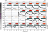 |
Fig. 11. Same as Fig. 10, but for FCC 170. This galaxy is dominated by an old central pressure-supported spheroidal component spanning ∼ 1 dex in metallicity. It has a secondary contribution from a progressively thinner and younger disk-like component, and a potential minor contribution from a warm metal-poor halo-like component. |
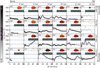 |
Fig. 12. Same as Fig. 10, but for FCC 177. This galaxy appears to have begun forming late. It is dominated by a young, thin disk, with contributions from dynamically-warmer and slightly older stars. |
The presence of cold kinematics and flattened (‘disk’-like) mass distributions are interpreted as in situ star formation, especially (though not necessarily) at high metallicity. Metal-rich and metal-poor stars in this regime would indicate that the gas likely originated from internal (recycling) and external (accretion) sources, respectively. This selection is in principle independent of age.
Centralised spheroidal distributions which are dynamically hot are interpreted as the in situ core or ‘bulge’. There is no strict selection on the stellar populations, since a large diversity has been observed in this region, especially if a stellar bar is or was present in the galaxy (Morelli et al. 2008, 2016; Coelho & Gadotti 2011; Zhao 2012; Florido et al. 2015; Seidel et al. 2015; Corsini et al. 2018). Orbits at large radius with hot kinematics and with metallicities towards the metal-poor tail of the host galaxy’s distribution are interpreted as the result of stellar accretion from many lower-mass systems. Such accretion is expected to be at least dynamically ‘warm’. This is because, although the impact of satellites may be preferentially along a particular axis (Shao et al. 2019), accreted stars would nevertheless be on dynamically hotter orbits compared to the in situ cold disk. In the event of minor merging, the accreted systems will, by definition, be lower mass than the host, and via the mass-metallicity relation will thus have lower metallicities on average. Since the age of the accreted stars depends critically on the SFH of the satellites, we make no selection on age for the ‘accreted’ stars. It is possible that some orbits in this regime have an in situ origin, from either past major mergers or significant external perturbations (since low-mass accretion events themselves are not expected to perturb the existing disk significantly; Hopkins et al. 2008). We nevertheless interpret this region as accretion under the assumption that it is dominated by ex situ material, subject to possible contamination by in situ material.
In the remainder of this section, the results are discussed briefly for each galaxy in the context of their individual assembly histories. We constrain the origin of dominant structures in each galaxy, which includes identifying the fraction of likely accreted material. Since the condition described above for the selection of accreted material favours orbits at larger radii, the limited spectroscopic FOV can bias these estimates. We instead estimate the accretion fraction as  , where the accreted stellar mass
  is approximated for each galaxy below, and the total enclosed stellar mass
  is given in Table 1. This proposed accreted fraction is discussed further in Sect. 5.
4.1. FCC 153
FCC 153 is suspected of being an ‘intermediate in-faller’ to the Fornax cluster (4 < tin−fall < 8 Gyr; as estimated from the cluster projected phase-space diagram in Iodice et al. 2019a). Figure 10 exhibits the largest spread of metallicity of the three galaxies studied here. FCC 153 also shows the strongest recent star-formation activity, having formed the most stellar mass (∼ 3 × 10⁹ M⊙) in recent times (< 6 Gyr), and in a kinematically-cold configuration. In fact, our model reveals that it has retained cold kinematics over all redshifts with even the oldest bins containing stars with σz ∼ 50 km s−1. The combination of late-time star-formation and persistent cold kinematics implies that the integrated assembly history of this galaxy (all mergers and interactions combined) has had a minimal impact, at least in the region covered by the spectroscopy. There is a suggestion of stellar accretion through the old, kinematically-warm, metal-poor population forming part of the stellar ‘halo’. We can use the model to estimate the mass in accreted stars by quantitatively isolating the orbits which meet the qualitative criteria discussed above. Specifically, orbits are selected with [Z/H] ≤ − 0.5 dex (lower half of Fig. 10), |λz| ≤ 0.5, and mean guiding radius  to exclude any potential in situ ‘bulge’-like orbits (see Fig. 4). This selection results in facc ∼ 10%. Under the assumption that these criteria isolate the accreted stars, we estimate an accreted mass of
  . This selection has a luminosity-weighted average age and metallicity of t = 11.8 Gyr and [Z/H] = −1.3 dex, respectively. Compared to the other two galaxies in this work, FCC 153 has the highest facc, and its relatively late in-fall may explain that. This is supported by the average age of the tentative accreted material, which implies that the main accretion events (those which dominate the luminosity-weighted average) occurred ≲ 11.8 Gyr ago.
4.2. FCC 170
FCC 170 is believed to be an ancient in-faller to the Fornax cluster (tin−fall > 8 Gyr; as estimated from the cluster projected phase-space diagram in Iodice et al. 2019a). It is the most distinct galaxy of those modelled in this work, being the most massive (Table 1). It is also believed to be situated closest to the cluster core. FCC 170 appears to have ceased the majority of its star formation the earliest, and its early in-fall and current position in the cluster likely played a role. The galaxy is very old, but we see evidence of recent star-formation, again in a cold configuration seemingly in spite of its environment (Fig. 11). Overall, FCC 170 has relatively-high velocity dispersion everywhere with respect to the other two galaxies. Yet the central regions (where we probe with the spectroscopy) have remained heavily rotationally-supported over its history, with σz ≲ 100 km s−1. Applying the same accretion criteria as for FCC 153, we estimate an accretion fraction of facc ∼ 7%, implying Macc ∼ 3 × 10⁹ M⊙ with a luminosity-weighted average age and metallicity of t = 13.3 Gyr and [Z/H] = −1.3 dex, respectively. With respect to FCC 153, this implies that FCC 170 experienced more accretion events of lower mass (lower metallicity).
4.3. FCC 177
FCC 177 is also believed to be an ancient in-faller (Iodice et al. 2019a), as for FCC 170. It has the lowest stellar mass and highest DM fraction of the three galaxies studied here (Table 1). It exhibits low velocity dispersion (σz < 100 km s−1) everywhere and at all times, with the younger, metal-rich populations reaching σz ≲ 20 km s−1 (Fig. 12). We find evidence for a delayed formation, with only a small fraction of old populations (t ≳ 312 Gyr) and without any clear spatial structures. At later times, FCC 177 appears to have sustained modest and roughly-constant star-formation for t ≲ 10 Gyr. This combination of prolonged star-formation and cold kinematics is especially surprising given its early in-fall, and poses problems for the expectation of group pre-processing and cluster quenching processes. The mass budget of FCC 177 is more complicated to disentangle, especially due to the relatively diffuse mass at old ages. In fact, FCC 177 has formed the largest percentage of its stellar mass in recent times, compared to the other two galaxies. Moreover, our assembly history indicates that for lookback times greater 10 Gyr ago, FCC 177 had just log10(M⋆/M⊙) ∼ 8, implying that the in situ component formed during that time would be lower metallicity with respect to the other two galaxies during the same period. This caveat notwithstanding, applying the same criteria as for the other galaxies, we estimate facc ∼ 6%. This results in  , with luminosity-weighted average age and metallicity of t = 12.8 Gyr and [Z/H] = −1.5 dex, respectively.
5. Mass assembly histories in context
In this section we review all the evidence afforded by this technique in the context of the Fornax cluster in order to investigate the dominant processes that built up the stellar mass in these galaxies. By analysing the trends in Figs. 10–12, and exploring them more quantitatively throughout this section, we can constrain certain formation mechanisms.
Interestingly, we see a diversity in the assembly histories of the three galaxies studied here via the different distributions of mass between Figs. 10–12. Yet the persistence of kinematically-cold orbits is common throughout all of the galaxies for all stellar ages. The observation of such kinematics for old populations places constraints on both internal and external disruption processes. Owing to the archaeological nature of the methodology employed here, all stars are observed in their present-day, not formation, configurations. It is clear, therefore, that in order for these orbits to remain kinematically-cold, those stars need to not only form as such, but also experience little-to-no subsequent disruption until the epoch of observation. This implies that neither internal instabilities nor the cluster potential (or other members) can cause significant perturbations to the kinematics of the central regions of these galaxies (though this is discussed further in Sects. 5.1 and 5.2). For the same reason, we argue that these galaxies have likely not experienced any high-mass-ratio mergers, as they would have similarly disrupted these old cold orbits (Hopkins et al. 2008).
There seems to be no lack of historic star-formation activity in these galaxies. This is perhaps most surprising for FCC 170 which exhibits by far the oldest mean stellar age, and is purported to reside in the central region of the cluster. We find evidence for the continued formation of stars in all three galaxies down to relatively young ages, and at super-solar metallicity. These episodes occurred comfortably after each galaxy is suspected to have entered the cluster. Their metallicity is consistent with self-enrichment, and thus in conjunction with their kinematics, these stars very likely formed in-situ from recycled gas.
The accretion of low-mass stellar systems is expected to deposit material into the outer stellar ‘halo’ regions of galaxies. It is also expected to contribute significantly to the present-day stellar mass of galaxies (Oser et al. 2010). We have estimated, however, low accretion fractions (<10%) for the galaxies studied here. There are two sources of uncertainty in the facc estimates in this work; contamination by in situ stars in the region we consider ‘accreted’, and excluding some accreted material which resides at lower radius. We can not strictly exclude an in situ contribution to these accretion fractions, but such contamination would imply an intrinsic accreted fraction even lower than estimated here. Without major mergers, any in situ stars that satisfy the proposed criteria for accretion are difficult to explain, unless external perturbations from the cluster have caused dramatic transformations. Moreover, Karademir et al. (2019) find that mergers with smaller mass ratios deposit stars at larger radii. Once again, since we have argued against major (or even a significant amount of minor) mergers, it is plausible that at least the majority of accretion for these galaxies resides at large radius. Davison et al. (2020) similarly find that for galaxies in the EAGLE simulation, most of the accreted mass is deposited beyond the half-mass radius r1/2 for host stellar masses within the range of our Fornax galaxies. We nevertheless caution that facc is subject to these uncertainties, and highlight that the other main conclusions of this work do not depend on the measurements of accretion. While the mass models are constrained over the full extent of the galaxies using the FDS photometry (Sect. 3.1), we can not exclude higher accretion fractions being found at larger radii as inferred by, for instance, Pulsoni et al. (2018) for the stellar mass range probed by our sample.
A lack of accretion can be explained by the high relative motions of member galaxies within a cluster, and reduced merging has been seen previously for cluster members with respect to the field (Berrier et al. 2008; Pipino et al. 2014). Specifically for the Fornax cluster, its members and their globular cluster (GC) populations have been analysed previously (Jordán et al. 2015; Fahrion et al. 2020). Fahrion et al. (2020) finds that FCC 170 has a significantly reduced number of GC for its stellar mass, and those that is has are notably metal-poor. While the numbers of GC for FCC 153 and FCC 177 are less unusual, since the hosts are themselves lower stellar mass, their GC are also more metal-poor compared to the stellar body by ∼ 1 dex. This implies that the GC originated in lower-mass systems. Once again, this suggests a lack of major mergers, and low incidence of minor merging for the three galaxies studied here. Low accretion fractions for these three galaxies were also inferred from the analysis of Pinna et al. (2019a). These galaxies appear to have been shut off from sources of external material by the cluster environment, which has likely stifled their growth. Their stellar mass assembly was able to continue through in situ star formation, but has ceased in the present day likely due to the exhaustion of internal gas in conjunction with the lack of replenishment.
5.1. The stellar age–velocity-dispersion relation
Here we quantitatively explore some of the correlations alluded to in the assembly histories. To this end, we investigate the vertical component of the intrinsic stellar velocity dispersion, σz, as a function of formation time of the stars (converted to redshift assuming the cosmology of Ade et al. 2016, as implemented in astropy). This stellar age–velocity-dispersion relation (AVR) has been studied previously in the Local Group (Wielen 1977; Nordström et al. 2004; Rocha-Pinto et al. 2004; Seabroke & Gilmore 2007; Martig et al. 2014; Sharma et al. 2014; Beasley et al. 2015; Hayden et al. 2017; Grieves et al. 2018; Bhattacharya et al. 2019; Mackereth et al. 2019) and a number of cosmological and idealised simulations (Bird et al. 2013; Aumer et al. 2016; Grand et al. 2016; Kumamoto et al. 2017). The gas-phase AVR is also well-studied (e.g., Wisnioski et al. 2015). While the stellar AVR is derived through the properties of stars of different ages within individual galaxies, in contrast, the gas-phase AVR is measured via the global properties of different galaxies observed directly at different redshifts. In all cases, σz is seen to decrease towards the present day, but with competing explanations as to the physical driver of this relation. It is often thought to be the result of either internal instabilities whose cumulative effects have disturbed older stars more (Saha et al. 2010; Aumer et al. 2016; Grand et al. 2016; Yu & Liu 2018) or that populations of stars which formed at high redshift inherited higher random motion from their surroundings, which has been decreasing towards the present day as conditions stabilise (Noguchi 1998; Bournaud et al. 2009; Bird et al. 2013; Leaman et al. 2017; Ma et al. 2017). Since the AVR pertains to the conditions which lead to star-formation, the measurements of these properties are restricted to the disk plane, as this is where in situ star-formation is expected to occur.
The stellar AVR measured in this work for the three Fornax galaxies are presented in Fig. 13, with comparisons to literature measurements. We track the velocity dispersion as a function of formation redshift, marginalised over metallicity and radius. That is, at fixed age, the metallicities are averaged according to their luminosity-weighted contribution to the model, then similarly for radius. This maintains the appropriate weighting such that the final σz measurements are also luminosity-weighted. For consistency with literature measurements, we measure these properties for the ‘disk’-like orbits of the models; that is, we consider only those orbits with |λz| ≥ 0.8. The resulting relations are shown by the large stars in Fig. 13. Additionally, the relations for all orbits (with no selection on circularity) are given by the dashed curves.
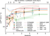 |
Fig. 13. Stellar disk AVR as derived from our models. The coloured stars are the galaxies modelled in this work (and Poci et al. 2019, for NGC 3115). The symbol size is proportional to the fractional stellar mass in each age bin, for each galaxy independently. The horizontal error-bars denote the width of the age bin. The vertical error bars are computed as the weighted standard deviation within each age bin, for the best-fit model. The shaded regions show the spread in σz for 100 Monte Carlo fits to the stellar-population maps. The dashed curves show the stellar AVR of the four S0 galaxies when all orbits are included (no selection on orbital circularity). The box-whisker plots are literature measurements of cold gas disks, from HERACLES (Leroy et al. 2009), DYNAMO (Green et al. 2014), GHASP (Epinat et al. 2010), PHIBBS (Tacconi et al. 2013), MASSIV (Epinat et al. 2012), OSIRIS (Law et al. 2009), AMAZE-LSD (Gnerucci et al. 2011), SINS (Schreiber et al. 2009) and zC-SINF (Schreiber et al. 2014), KMOS3D (Wisnioski et al. 2015), and KDS (Turner et al. 2017). The black dots and crosses are Milky-Way stellar measurements (Yu & Liu 2018) for stars on (|z| < 270 pc) and off (|z| > 270 pc) the plane, respectively. Galaxy disks become dynamically colder towards the present day. The cluster S0 galaxies have a higher contribution from warmer orbits at more recent times compared to the field galaxy (comparing the full and disk-only σz). The Milky-Way, despite its higher stellar mass, is dynamically colder than the S0 galaxies studied here. |
All of these galaxies show the same general trend of decreasing σz with decreasing stellar age. The trends we measure for the stellar σz are flatter than those for direct gas measurements, as the stars do not reach the coldest dynamical temperatures observed in gas in the present day. This is in agreement with predictions from simulations (Pillepich et al. 2019). We also see that the field galaxy NGC 3115, despite being two times more massive than our most massive Fornax object, exhibits comparable vertical velocity dispersion. By comparing the disk AVR to the full-orbit AVR, it can be seen that all three Fornax galaxies show a measurable contribution from non-disk-like orbits at all ages. Together, these observations imply that we are likely measuring the impact of the cluster on the dynamics of its galaxies due to so-called ‘harassment’ (Moore et al. 1996); frequent though minor gravitational interactions between galaxies in close proximity. External perturbations have also been seen to cause heating coincident with the time of the interaction (Grand et al. 2016).
Our results are also compared in Fig. 13 to data from the Milky-Way, both on (|z| < 270 pc) and off (|z| > 270 pc) the disk plane (Yu & Liu 2018). For comparison, the physical pixel scale of the data used in this work is ∼ 20 pc pixel−1, but with a real physical resolution of ∼ 70 pc due to the point-spread function of the observations. So while our models are not separated based on height above the plane, they still probe the most dynamically-cold physical scales, meaning that any differences between these results are not due to spatial resolution effects. All four S0 galaxies exhibit a systematic increase of σz with respect to the Milky-Way, which is expected since galaxies that can support spiral arms should be dynamically colder. In this case, the offset is likely a combination of the different morphology and environment, yet the general shape of the relation is preserved despite these differences.
As discussed above, each galaxy retains a significant portion of mass with cold kinematics and disk-like morphology at the oldest age. Specifically, these oldest age bins (as seen in the present day) exhibit σz ∼ 50 km s−1 on the disk plane at intermediate radii and high metallicity. This is inconsistent with internal heating whose effect should be maximal for the oldest stars. For instance, the simulations of Aumer et al. (2016) show that for the oldest stars, internal heating will increase σz by ∼ 15−20 km s−1 above the value at birth. For the old stars we measure in the present day which have σz ∼ 50 km s−1, this would imply that they were born with σz ∼ 30−35 km s−1 at z = 4−5, which is significantly lower than the gas measurements at that epoch. Therefore, we conclude that the AVR for these galaxies is the result of hotter dynamical temperatures at early times, while further minor heating is contributed by the cluster interactions.
Closer inspection of Figs. 10–12 indicates a 3D correlation between mean σz, stellar age, and stellar metallicity, yet the results of Fig. 13 marginalise over metallicity. We therefore compute these relations without such marginalisation, to investigate the impact of age and metallicity independently. These are presented in Fig. 14. In order to avoid numerical noise which could be introduced through the increasingly-complex selection criteria, we conduct this analysis on the full diversity of orbits (without selecting on circularity). The curves in Fig. 14 are constructed by collecting individual rows and columns of Figs. 10–12. Each panel of those figures is integrated along the radial profile, preserving the luminosity weighting at each point, to produce a single σz measurement for that panel. Each row in the assembly histories corresponds to a single curve of the AVR at fixed metallicity (left column of Fig. 14), while each column in the assembly histories corresponds to a single curve of the [Z/H] − σz relation at fixed age (right column of Fig. 14). The Spearman rank correlation coefficient r, which indicates the strength and direction of a trend, is computed using the scipy implementation for all curves in a given panel. The corresponding p-value is also shown for each panel, which indicates the probability that the two axes are uncorrelated.
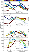 |
Fig. 14. Correlations of σz with stellar age at fixed metallicity (left), and stellar metallicity at fixed age (right) for, from top to bottom, the three galaxies studied in this work, and the field S0 NGC 3115 (Poci et al. 2019). The curves are coloured by their age/metallicity bin corresponding to those of Figs. 10–12. The Spearman rank coefficient r and the associated p-value, computed for all curves collectively in a given panel, are inset. The shaded regions correspond to the variations derived from 100 Monte Carlo fits to the stellar population maps. The stellar AVR at fixed metallicity exhibits lower significance than the [Z/H] − σz at fixed age. |
We observe a significant [Z/H] − σz correlation at fixed age, such that the more metal-poor stars are dynamically hotter. Similar correlations between the metallicity and vertical velocity dispersion have been seen previously for the Milky-Way (for the iron abundance [Fe/H], and typically with non-trivial selection functions; Meusinger et al. 1991; Ness et al. 2013; Minchev et al. 2014; Grieves et al. 2018; Arentsen et al. 2020) and for M 31 (Dorman et al. 2015) but those results are marginalised over age. Similarly, all previous studies of the stellar AVR have been marginalised over metallicity – with the exception of Sharma et al. (2020), discussed below. Interestingly, Guiglion et al. (2015) see the inverse trend of σz with [Mg/Fe] at fixed [Fe/H] for the Milky-Way. Figure 14 shows that the AVR is a weak correlation once metallicity is accounted for, quantified by the correlation coefficients in each case. At fixed age, the [Z/H] − σz relation is significantly more correlated than the AVR at fixed metallicity. We emphasise that the stellar AVR in Fig. 13 (even the dashed full-orbit curves) exhibits a correlation which is consistent with previous measurements when metallicity is not taken into account. This means that the result in Fig. 14 can not be due to any degeneracy between age and metallicity in our models. Furthermore, age and metallicity are fit independently in Sect. 3.4, and the spatial coherence of the dynamical components (each spatial bin is not independent) is exploited to reduce possible degeneracies within each fit. At face value, this result implies that [Z/H] − σz is the underlying physical correlation, while the impact of age (or formation redshift) is of secondary importance. In this scenario, the stellar AVR would manifest through the age-metallicity relation and its scatter. Finally, while the results in Fig. 14 include the full diversity of orbits from our models, we confirmed, by removing the suspected accretion components (via the same selection identified in Sect. 4) that neither the direction nor the relative significance of these correlations change. This implies that the results of Fig. 14 are not merely driven by the fact that accreted material is often dynamically hotter and relatively metal-poor, but rather that it is inherent to what we identify as the in situ component.
We posit that the [Z/H] − σz relation is driven by the successive ‘generations’ of star formation, each becoming more enriched and more dynamically-cold than those before (in the absence of accretion which would result in the chemical and dynamical mixing of the populations). This could be the case if, for instance, mass segregation of metals occurs vertically as well as radially. Alternatively, this would be the result if higher-metallicity gas requires colder kinematics before star formation is possible, or if the cooling effects of metals naturally produces more dynamically-cold disks if the gas is more metal-rich. Choi & Nagamine (2009) show that metal cooling can significantly increase the star-formation efficiency of the inter-stellar medium, though there is no direct link in that work to dynamics.
Yet measurements of the gas-phase AVR show clear trends with redshift, and the physical interpretation in that case explicitly includes a redshift dependence. However this redshift dependence is via gas depletion through the cosmic specific SFR (such as in Whitaker et al. 2014); in that scenario, galaxies with larger gas fractions experience larger inter-stellar medium turbulence, and higher σz is imparted to the stars upon star formation (Leaman et al. 2017). So in much the same way as the scenario proposed here for the stellar AVR, the gas-phase AVR is tied to episodes of star formation, which happen to decline on average with redshift. This subtle difference is especially important when analysing individual galaxies with individual assembly histories. There also remains significant scatter at fixed redshift within the gas-phase AVR that needs to be accounted for, which indicates a potential additional dimension to this issue. Naturally, these star-formation episodes lead to enrichment of the gas over cosmic time (Daigne et al. 2006; Kobayashi et al. 2007). Therefore, if metallicity is the underlying physical driver of the gas-phase AVR, it would still manifest as an observed redshift dependence without intrinsically depending on redshift directly. But this is only, at present, a circumstantial argument in lieu of an explicit experiment for gas disks.
In any case, a testable prediction of this hypothesis is that at fixed present-day stellar mass (and without significant ex situ contributions or perturbations), galaxies with higher SFR (that is, faster chemical enrichment) should achieve dynamically-colder orbits at fixed age – or alternatively, the stellar AVR should have a steeper slope. This is because in such a scenario, the absolute cosmic time is not the driver of the AVR, but rather the time it takes for a particular galaxy to achieve a particular degree of enrichment. Since the stellar metallicity and σz will depend on both stellar mass and accretion history, it is imperative to control for those parameters to test this prediction. This is at present not possible for the sample of galaxies for which our analysis has been performed, but should be accessible to theoretical models and simulations. In fact, Just & Jahreiß (2010) explicitly investigate the effect of SFR on the stellar AVR, tailored to fit the Milky-Way, through a series of models. That work finds that for similar forms of the SFH, the model with a higher SFR has lower vertical velocity dispersion, despite peaking at earlier epochs.
The outlier in this respect from Fig. 14 is NGC 3115. We have already established that accretion has played a minor role in the stellar mass assembly of the three Fornax galaxies. Conversely, Poci et al. (2019) conclude that NGC 3115 assembled ∼ 68% of its present-day stellar mass from external sources. Moreover, given the higher stellar mass of NGC 3115, these accreted systems could be higher mass, and therefore more enriched on average, compared to lower-mass satellites accreted onto lower-mass hosts. Thus the age and metallicity trends would be significantly phase-mixed, as is seen by the reduced correlation coefficients. The persistence of an AVR, only at high metallicity, may be indicative of secular evolution following the last accretion event.
A similar analysis has been performed for the Milky-Way using a combination of many of the recent photometric and spectroscopic surveys (Sharma et al. 2020). That work finds a strong [Z/H] − σz relation at fixed age. Yet they also find a persistent stellar AVR at fixed metallicity, but only at young ages. The AVR then flattens and correlates solely with metallicity at old ages. Yu & Liu (2018) see similar trends with two bins of metallicity. Sharma et al. (2020) interpret the [Z/H] − σz correlation as a connection between σz and the stellar birth radius. However, in the case of the Fornax galaxies, we see no clear (monotonic) radial gradients of metallicity in Figs. 7–9. Comparisons to that work are complicated, however, by the selection functions of the Milky-Way data sets, and so these results may be tracing different physical regimes.
5.2. S0 formation
All of our results indicate that the Fornax galaxies have undergone mild transformations due to the cluster potential, primarily in their outer regions. They have been able to retain their cold central kinematics, yet in a thicker configuration compared to the field. We posit, thus, that their S0 morphology is a result of these interactions. This is neither of the explanations typically invoked to explain the transformations of galaxies into S0; mergers (Chilingarian et al. 2009; Querejeta et al. 2015; Tapia et al. 2017; Poci et al. 2019) or the ‘fading’ of spiral galaxies (Larson et al. 1980; Bekki et al. 2002; D’Onofrio et al. 2015; Mishra et al. 2018; Rizzo et al. 2018). While cluster environments are common in the faded-spiral scenario, it is predicated on the supposed spiral progenitor first ceasing star-formation due to the environment (for instance, Boselli & Gavazzi 2006; Book & Benson 2010; Peng et al. 2012; Mendel et al. 2013; Bekki 2014), allowing it to subsequently transform into an S0 galaxy. Yet we see evidence for significant star formation activity well beyond the suspected time of in-fall to the cluster for all three galaxies. Gas was therefore readily available until relatively recently. The evidence for a lack of stellar accretion has been discussed, in agreement with other cluster studies, rendering this formation path unlikely as well. This is also consistent with the deductions of Comerón et al. (2019) and Pinna et al. (2019a) who find that accretion does not play a major role in the formation of ‘thick’ disks in local galaxies.
An alternative scenario proposed by Diaz et al. (2018) states that at high redshift, gas-rich satellite accretion onto compact elliptical galaxies leads to the formation of the disk component of the resulting S0. Our models impose the constraint that if this scenario occurred for the three Fornax galaxies, such accretion would have had to occur ≳ 12 Gyr ago for FCC 153 and FCC 170, and ≳ 10 Gyr ago for FCC 177, since it must precede the formation of the dynamically-cold disk. However, this scenario supposes that the compact elliptical, which goes on to form the ‘bulge’ of the subsequent S0, is responsible for the suppression of spiral arms in the disk. Conversely, our data suggest that only FCC 170 has a significant contribution from a central pressure-supported structure. More broadly, a diversity of S0 properties is emerging (Fraser-McKelvie et al. 2018; Coccato et al. 2020; Deeley et al. 2020; Tous et al. 2020), and it is unlikely that a single formation path is responsible for this diversity.
5.3. The Fornax galaxy cluster population
The photometric catalogue of Ferguson (1989), covering 40 sq. deg., contains 35 S0-like galaxies (some of which have uncertain classification), with 20 being brighter than the magnitude limit of the Fornax3D survey (mB ≤ 15). Of these, 12 were observed by Fornax3D, accounting for 60% (34%) of bright (all) lenticular galaxies in the Fornax cluster. Our analysis on the sub-sample of three galaxies, chosen for the reasons discussed above, can not therefore account for the expected diversity of evolutionary pathways within the cluster’s galaxy population. So while we infer no major mergers for these galaxies, for instance, we can not exclude this formation path for some of the other cluster S0 galaxies. We have, however, probed the relative extremes in terms of assembly histories, with FCC 170 and FCC 177 forming the majority of their stellar content at early and late times, respectively. This analysis has simultaneously uncovered properties which appear to be approximately independent of assembly history – namely the stellar AVR – which we thus expect to hold for all but the most violent histories. To confidently infer the histories of the remaining galaxies from Fornax3D, this analysis must be applied to each of them individually. This is the goal of future work.
6. Conclusions
In this work we modelled three edge-on S0 galaxies in the Fornax cluster as part of the Fornax3D project. We applied sophisticated dynamical and stellar-population techniques to self-consistently model the entire stellar information content. These models were used to infer how each galaxy formed, and allowed us to place strong constraints on some of the hypothesised processes that affect galaxy formation and evolution, in particular in the cluster environment. These findings are summarised here:
-
All three galaxies retain a strongly-rotating component that has persisted for many dynamical times. These structures can be composed of both young and old stars, implying that they have survived the galaxy’s entry into the cluster and subsequent evolution therein (Figs. 10–12).
-
There is evidence of continued star-formation in all three galaxies, to varying degrees. Owing to the metallicity and kinematics, we suggest this star formation is almost exclusively in-situ through recycled gas, as there is no evidence of gas accretion (Figs. 10–12).
-
Our results are suggestive of a suppression of stellar accretion. We postulate that this is driven by the relative motions of galaxies within the cluster (Figs. 10–12), as proposed in previous works.
-
There is evidence against internal heating as the cause of the stellar age–velocity-dispersion relation, suggesting that older stars were created with inherently-higher σz, in agreement with the results of Poci et al. (2019). There is tentative evidence that the relations for the cluster galaxies are elevated with respect to the field (Fig. 13), implying that harassment may be responsible for mild dynamical heating.
-
We find tentative observational evidence of a potential fundamental stellar [Z/H] − σz relation which we argue may contribute significantly to the observed age–velocity-dispersion relation (Fig. 14).
We endeavour in future work to incorporate more detailed stellar-population analyses, including variable IMF, while continuing to apply this methodology to a variety of galaxies. Deriving these histories for other galaxies will enable a more thorough understanding of how galaxies piece together their mass, and which processes have dominant effects in various regimes.
Available at https://pypi.org/project/vorbin/
Available at https://pypi.org/project/ppxf/
Available at https://pypi.org/project/mgefit/
Using the plotbin package, available at https://pypi.org/project/plotbin/
Acknowledgments
We thank Lorenzo Morelli, Thomas Spriggs, and Adrian Bittner for discussions on this work. AP acknowledges financial support from Macquarie University and the ESO Studentship Programme. RMM is the recipient of an Australian Research Council Future Fellowship (project number FT150100333). LZ acknowledges the support from National Natural Science Foundation of China under grant No. Y945271001, and the National Key R&D Program of China under grant No. 2018YFA0404501. GvdV acknowledges funding from the European Research Council (ERC) under the European Union’s Horizon 2020 research and innovation programme under grant agreement no. 724857 (Consolidator Grant ArcheoDyn). EMC is supported by MIUR grant PRIN 2017 20173ML3WW_001 and by Padua University grants DOR1715817/17, DOR1885254/18, and DOR1935272/19. JF-B, IMN, and FP acknowledge support through the RAVET project by the grant PID2019-107427GB-C32 from The Spanish Ministry of Science and Innovation. Based on observations collected at the European Southern Observatory under ESO programme 296.B-5054(A). This work makes use of the SciGar compute cluster at ESO, and the OzStar supercomputer at Swinbourne University. The work also makes use of existing software packages for data analysis and presentation, including ASTROPY (Astropy Collaboration 2013), CYTHON (Behnel et al. 2011), IPYTHON (Perez & Granger 2007), MATPLOTLIB (Hunter 2007), NUMPY (Harris et al. 2020), the SCIPY ecosystem (Virtanen et al. 2020), and STATSMODELS (Seabold & Perktold 2010). We finally thank the anonymous referee, whose feedback greatly improved the depth and clarity of this work.
References
- Ade, P. A. R., Aghanim, N., Arnaud, M., et al. 2016, A&A, 594, A13 [NASA ADS] [CrossRef] [EDP Sciences] [Google Scholar]
- Allen, R. J., Kacprzak, G. G., Glazebrook, K., et al. 2016, ApJ, 826, 60 [Google Scholar]
- Alpaslan, M., Driver, S., Robotham, A. S. G., et al. 2015, MNRAS, 451, 3249 [NASA ADS] [CrossRef] [Google Scholar]
- Arentsen, A., Starkenburg, E., Martin, N. F., et al. 2020, MNRAS, 491, L11 [CrossRef] [Google Scholar]
- Asa’d, R., & Goudfrooij, P. 2020, MNRAS, 498, 2814 [Google Scholar]
- Astropy Collaboration (Robitaille, T. P., et al.) 2013, A&A, 558, A33 [NASA ADS] [CrossRef] [EDP Sciences] [Google Scholar]
- Aumer, M., Binney, J., & Schönrich, R. 2016, MNRAS, 462, 1697 [NASA ADS] [CrossRef] [Google Scholar]
- Balogh, M., Eke, V., Miller, C., et al. 2004, MNRAS, 348, 1355 [Google Scholar]
- Beasley, M. A., San Roman, I., Gallart, C., Sarajedini, A., & Aparicio, A. 2015, MNRAS, 451, 3400 [NASA ADS] [CrossRef] [Google Scholar]
- Behnel, S., Bradshaw, R., Citro, C., et al. 2011, Comput. Sci. Eng., 13, 31 [Google Scholar]
- Bekki, K. 2014, MNRAS, 438, 444 [NASA ADS] [CrossRef] [Google Scholar]
- Bekki, K., Couch, W. J., & Shioya, Y. 2002, ApJ, 577, 651 [NASA ADS] [CrossRef] [Google Scholar]
- Bellstedt, S., Forbes, D. A., Romanowsky, A. J., et al. 2018, MNRAS, 476, 4543 [NASA ADS] [CrossRef] [Google Scholar]
- Berrier, J. C., Stewart, K. R., Bullock, J. S., et al. 2008, ApJ, 690, 1292 [Google Scholar]
- Bhattacharya, S., Arnaboldi, M., Caldwell, N., et al. 2019, A&A, 631, A56 [NASA ADS] [CrossRef] [EDP Sciences] [Google Scholar]
- Bird, J. C., Kazantzidis, S., Weinberg, D. H., et al. 2013, ApJ, 773, 43 [NASA ADS] [CrossRef] [MathSciNet] [Google Scholar]
- Blakeslee, J. P., Jordán, A., Mei, S., et al. 2009, ApJ, 694, 556 [NASA ADS] [CrossRef] [Google Scholar]
- Blanton, M. R., Eisenstein, D., Hogg, D. W., Schlegel, D. J., & Brinkmann, J. 2005, ApJ, 629, 143 [NASA ADS] [CrossRef] [Google Scholar]
- Book, L. G., & Benson, A. J. 2010, ApJ, 716, 810 [NASA ADS] [CrossRef] [Google Scholar]
- Boselli, A., & Gavazzi, G. 2006, PASP, 118, 517 [NASA ADS] [CrossRef] [Google Scholar]
- Bournaud, F., Elmegreen, B. G., & Martig, M. 2009, ApJ, 707, L1 [NASA ADS] [CrossRef] [Google Scholar]
- Brough, S., van de Sande, J., Owers, M. S., et al. 2017, ApJ, 844, 59 [NASA ADS] [CrossRef] [Google Scholar]
- Cappellari, M. 2002, MNRAS, 333, 400 [NASA ADS] [CrossRef] [Google Scholar]
- Cappellari, M. 2016, ARA&A, 54, 597 [NASA ADS] [CrossRef] [Google Scholar]
- Cappellari, M. 2017, MNRAS, 466, 798 [NASA ADS] [CrossRef] [Google Scholar]
- Cappellari, M., & Copin, Y. 2003, MNRAS, 342, 345 [NASA ADS] [CrossRef] [Google Scholar]
- Cappellari, M., & Emsellem, E. 2004, PASP, 116, 138 [NASA ADS] [CrossRef] [Google Scholar]
- Cappellari, M., Bacon, R., Bureau, M., et al. 2006, MNRAS, 366, 1126 [NASA ADS] [CrossRef] [Google Scholar]
- Cappellari, M., Emsellem, E., Krajnović, D., et al. 2011a, MNRAS, 416, 1680 [NASA ADS] [CrossRef] [Google Scholar]
- Cappellari, M., Emsellem, E., Krajnović, D., et al. 2011b, MNRAS, 413, 813 [NASA ADS] [CrossRef] [Google Scholar]
- Cappellari, M., McDermid, R. M., Alatalo, K., et al. 2012, Nature, 484, 485 [NASA ADS] [CrossRef] [Google Scholar]
- Cappellari, M., McDermid, R. M., Alatalo, K., et al. 2013, MNRAS, 432, 1862 [Google Scholar]
- Chilingarian, I. V., Novikova, A. P., Cayatte, V., et al. 2009, A&A, 504, 389 [NASA ADS] [CrossRef] [EDP Sciences] [Google Scholar]
- Choi, J.-H., & Nagamine, K. 2009, MNRAS, 393, 1595 [Google Scholar]
- Choi, H., Yi, S. K., Dubois, Y., et al. 2018, ApJ, 856, 114 [Google Scholar]
- Christlein, D., & Zabludoff, A. I. 2005, ApJ, 621, 201 [NASA ADS] [CrossRef] [Google Scholar]
- Coccato, L., Jaffé, Y. L., Cortesi, A., et al. 2020, MNRAS, 492, 2955 [Google Scholar]
- Coelho, P., & Gadotti, D. A. 2011, ApJ, 743, L13 [Google Scholar]
- Cole, D. R., & Binney, J. 2017, MNRAS, 465, 798 [NASA ADS] [CrossRef] [Google Scholar]
- Cole, J., Bezanson, R., van der Wel, A., et al. 2020, ApJ, 890, L25 [Google Scholar]
- Comerón, S., Salo, H., Knapen, J. H., & Peletier, R. F. 2019, A&A, 623, A89 [NASA ADS] [CrossRef] [EDP Sciences] [Google Scholar]
- Corsini, E. M., Morelli, L., Zarattini, S., et al. 2018, A&A, 618, A172 [NASA ADS] [CrossRef] [EDP Sciences] [Google Scholar]
- Cortese, L., van de Sande, J., Lagos, C. P., et al. 2019, MNRAS, 485, 2656 [NASA ADS] [CrossRef] [Google Scholar]
- Cretton, N., de Zeeuw, P. T., van der Marel, R. P., & Rix, H.-W. 1999, ApJS, 124, 383 [NASA ADS] [CrossRef] [Google Scholar]
- Cretton, N., Rix, H.-W., & de Zeeuw, P. T. 2000, ApJ, 536, 319 [NASA ADS] [CrossRef] [Google Scholar]
- Daigne, F., Olive, K. A., Silk, J., Stoehr, F., & Vangioni, E. 2006, ApJ, 647, 773 [NASA ADS] [CrossRef] [Google Scholar]
- Davies, J. I., Bianchi, S., Baes, M., et al. 2013, MNRAS, 428, 834 [NASA ADS] [CrossRef] [Google Scholar]
- Davison, T. A., Norris, M. A., Pfeffer, J. L., Davies, J. J., & Crain, R. A. 2020, MNRAS, 497, 81 [Google Scholar]
- Deeley, S., Drinkwater, M. J., Sweet, S. M., et al. 2020, MNRAS, 498, 2372 [Google Scholar]
- Diaz, J., Bekki, K., Forbes, D. A., et al. 2018, MNRAS, 477, 2030 [Google Scholar]
- D’Onofrio, M., Marziani, P., & Buson, L. 2015, Front. Space Sci. Astron, 2, 4 [Google Scholar]
- Dorman, C. E., Guhathakurta, P., Seth, A. C., et al. 2015, ApJ, 803, 24 [NASA ADS] [CrossRef] [Google Scholar]
- Dressler, A. 1980, ApJ, 236, 351 [NASA ADS] [CrossRef] [Google Scholar]
- Drinkwater, M. J., Gregg, M. D., & Colless, M. 2001, ApJ, 548, L139 [NASA ADS] [CrossRef] [Google Scholar]
- Du, W., & McGaugh, S. S. 2020, AJ, 160, 122 [Google Scholar]
- Emsellem, E., Monnet, G., & Bacon, R. 1994, A&A, 285, 723 [NASA ADS] [Google Scholar]
- Epinat, B., Amram, P., Balkowski, C., & Marcelin, M. 2010, MNRAS, 401, 2113 [NASA ADS] [CrossRef] [Google Scholar]
- Epinat, B., Tasca, L., Amram, P., et al. 2012, A&A, 539, A92 [NASA ADS] [CrossRef] [EDP Sciences] [Google Scholar]
- Fahrion, K., Müller, O., Rejkuba, M., et al. 2020, A&A, 634, A53 [CrossRef] [EDP Sciences] [Google Scholar]
- Falcón-Barroso, J., Sánchez-Blázquez, P., Vazdekis, A., et al. 2011, A&A, 532, A95 [NASA ADS] [CrossRef] [EDP Sciences] [Google Scholar]
- Ferguson, H. C. 1989, AJ, 98, 367 [Google Scholar]
- Florido, E., Zurita, A., Pérez, I., et al. 2015, A&A, 584, A88 [NASA ADS] [CrossRef] [EDP Sciences] [Google Scholar]
- Fraser-McKelvie, A., Aragón-Salamanca, A., Merrifield, M., et al. 2018, MNRAS, 481, 5580 [NASA ADS] [CrossRef] [Google Scholar]
- Gargiulo, A., Cucciati, O., Garilli, B., et al. 2019, A&A, 631, A15 [Google Scholar]
- Gebhardt, K., Richstone, D., Tremaine, S., et al. 2003, ApJ, 583, 92 [NASA ADS] [CrossRef] [Google Scholar]
- Gnerucci, A., Marconi, A., Cresci, G., et al. 2011, A&A, 528, A88 [NASA ADS] [CrossRef] [EDP Sciences] [Google Scholar]
- Goddard, D., Thomas, D., Maraston, C., et al. 2017, MNRAS, 465, 688 [NASA ADS] [CrossRef] [Google Scholar]
- Graham, M. T., Cappellari, M., Bershady, M. A., & Drory, N. 2019, ArXiv e-prints [arXiv:1910.05139] [Google Scholar]
- Grand, R. J. J., Springel, V., Gómez, F. A., et al. 2016, MNRAS, 459, 199 [NASA ADS] [CrossRef] [Google Scholar]
- Grand, R. J. J., Gómez, F. A., Marinacci, F., et al. 2017, MNRAS, 467, 179 [NASA ADS] [Google Scholar]
- Green, A. W., Glazebrook, K., McGregor, P. J., et al. 2014, MNRAS, 437, 1070 [NASA ADS] [CrossRef] [Google Scholar]
- Grieves, N., Ge, J., Thomas, N., et al. 2018, MNRAS, 481, 3244 [NASA ADS] [CrossRef] [Google Scholar]
- Guiglion, G., Recio-Blanco, A., de Laverny, P., et al. 2015, A&A, 583, A91 [NASA ADS] [CrossRef] [EDP Sciences] [Google Scholar]
- Gunn, J. E., & Gott, J. R., III 1972, ApJ, 176, 1 [Google Scholar]
- Harris, C. R., Millman, K. J., van der Walt, S. J., et al. 2020, Nature, 585, 357 [CrossRef] [PubMed] [Google Scholar]
- Hayden, M. R., Recio-Blanco, A., de Laverny, P., Mikolaitis, S., & Worley, C. C. 2017, A&A, 608, L1 [NASA ADS] [CrossRef] [EDP Sciences] [Google Scholar]
- Hopkins, P. F., Hernquist, L., Cox, T. J., Younger, J. D., & Besla, G. 2008, ApJ, 688, 757 [NASA ADS] [CrossRef] [Google Scholar]
- Hunter, J. D. 2007, Comput. Sci. Eng., 9, 90 [NASA ADS] [CrossRef] [Google Scholar]
- Iodice, E., Capaccioli, M., Grado, A., et al. 2016, ApJ, 820, 42 [NASA ADS] [CrossRef] [Google Scholar]
- Iodice, E., Spavone, M., Cantiello, M., et al. 2017, ApJ, 851, 75 [Google Scholar]
- Iodice, E., Sarzi, M., Bittner, A., et al. 2019a, A&A, 627, A136 [NASA ADS] [CrossRef] [EDP Sciences] [Google Scholar]
- Iodice, E., Spavone, M., Capaccioli, M., et al. 2019b, A&A, 623, A1 [NASA ADS] [CrossRef] [EDP Sciences] [Google Scholar]
- Jin, Y., Zhu, L., Long, R. J., et al. 2019, MNRAS, 486, 4753 [CrossRef] [Google Scholar]
- Jordán, A., Blakeslee, J. P., Côté, P., et al. 2007, ApJS, 169, 213 [NASA ADS] [CrossRef] [Google Scholar]
- Jordán, A., Peng, E. W., Blakeslee, J. P., et al. 2015, ApJS, 221, 13 [NASA ADS] [CrossRef] [Google Scholar]
- Just, A., & Jahreiß, H. 2010, MNRAS, 402, 461 [Google Scholar]
- Karademir, G. S., Remus, R.-S., Burkert, A., et al. 2019, MNRAS, 487, 318 [NASA ADS] [CrossRef] [Google Scholar]
- Kauffmann, G., White, S. D. M., Heckman, T. M., et al. 2004, MNRAS, 353, 713 [NASA ADS] [CrossRef] [Google Scholar]
- Kobayashi, C., Springel, V., & White, S. D. M. 2007, MNRAS, 376, 1465 [Google Scholar]
- Kormendy, J., & Ho, L. C. 2013, ARA&A, 51, 511 [Google Scholar]
- Krajnović, D., McDermid, R. M., Cappellari, M., & Davies, R. L. 2009, MNRAS, 399, 1839 [NASA ADS] [CrossRef] [Google Scholar]
- Krajnović, D., Weilbacher, P. M., Urrutia, T., et al. 2015, MNRAS, 452, 2 [NASA ADS] [CrossRef] [Google Scholar]
- Kroupa, P. 2002, Science, 295, 82 [Google Scholar]
- Kumamoto, J., Baba, J., & Saitoh, T. R. 2017, PASJ, 69, 32 [Google Scholar]
- Larson, R. B., Tinsley, B. M., & Caldwell, C. N. 1980, ApJ, 237, 692 [NASA ADS] [CrossRef] [Google Scholar]
- Law, D. R., Steidel, C. C., Erb, D. K., et al. 2009, ApJ, 697, 2057 [Google Scholar]
- Lawson, C. L., & Hanson, R. J. 1995, Solving Least Squares Problems, Classics in Applied Mathematics (Philadelphia: Society for Industrial and Applied Mathematics) [Google Scholar]
- Leaman, R., Mendel, J. T., Wisnioski, E., et al. 2017, MNRAS, 472, 1879 [Google Scholar]
- Leroy, A. K., Walter, F., Bigiel, F., et al. 2009, AJ, 137, 4670 [NASA ADS] [CrossRef] [Google Scholar]
- Leung, G. Y. C., Leaman, R., van de Ven, G., et al. 2018, MNRAS, 477, 254 [NASA ADS] [CrossRef] [Google Scholar]
- Li, C., Zhu, L., Long, R. J., et al. 2020, MNRAS, 492, 2775 [Google Scholar]
- Lyubenova, M., van den Bosch, R. C. E., Côté, P., et al. 2013, MNRAS, 431, 3364 [NASA ADS] [CrossRef] [Google Scholar]
- Lyubenova, M., Martín-Navarro, I., van de Ven, G., et al. 2016, MNRAS, 463, 3220 [NASA ADS] [CrossRef] [Google Scholar]
- Ma, X., Hopkins, P. F., Wetzel, A. R., et al. 2017, MNRAS, 467, 2430 [Google Scholar]
- Mackereth, J. T., Schiavon, R. P., Pfeffer, J., et al. 2019, MNRAS, 482, 3426 [NASA ADS] [CrossRef] [Google Scholar]
- Martig, M., Minchev, I., & Flynn, C. 2014, MNRAS, 443, 2452 [NASA ADS] [CrossRef] [Google Scholar]
- Martín-Navarro, I., Lyubenova, M., van de Ven, G., et al. 2019, A&A, 626, A124 [NASA ADS] [CrossRef] [EDP Sciences] [Google Scholar]
- McDermid, R. M., Alatalo, K., Blitz, L., et al. 2015, MNRAS, 448, 3484 [NASA ADS] [CrossRef] [Google Scholar]
- McGaugh, S. S., & Schombert, J. M. 2014, AJ, 148, 77 [NASA ADS] [CrossRef] [Google Scholar]
- Mendel, J. T., Simard, L., Ellison, S. L., & Patton, D. R. 2013, MNRAS, 429, 2212 [Google Scholar]
- Meusinger, H., Reimann, H. G., & Stecklum, B. 1991, A&A, 245, 57 [Google Scholar]
- Minchev, I., Chiappini, C., Martig, M., et al. 2014, ApJ, 781, L20 [NASA ADS] [CrossRef] [Google Scholar]
- Mishra, P. K., Wadadekar, Y., & Barway, S. 2018, MNRAS, 478, 351 [Google Scholar]
- Monnet, G., Bacon, R., & Emsellem, E. 1992, A&A, 253, 366 [NASA ADS] [Google Scholar]
- Moore, B., Katz, N., Lake, G., Dressler, A., & Oemler, A. 1996, Nature, 379, 613 [NASA ADS] [CrossRef] [Google Scholar]
- Morelli, L., Pompei, E., Pizzella, A., et al. 2008, MNRAS, 389, 341 [NASA ADS] [CrossRef] [Google Scholar]
- Morelli, L., Parmiggiani, M., Corsini, E. M., et al. 2016, MNRAS, 463, 4396 [NASA ADS] [CrossRef] [Google Scholar]
- Muñoz, R. P., Eigenthaler, P., Puzia, T. H., et al. 2015, ApJ, 813, L15 [NASA ADS] [CrossRef] [Google Scholar]
- Navarro, J. F., Frenk, C. S., & White, S. D. M. 1996, ApJ, 462, 563 [Google Scholar]
- Ness, M., Freeman, K., Athanassoula, E., et al. 2013, MNRAS, 432, 2092 [NASA ADS] [CrossRef] [Google Scholar]
- Nguyen, D. D., Seth, A. C., Neumayer, N., et al. 2019, ApJ, 872, 104 [NASA ADS] [CrossRef] [Google Scholar]
- Nitschai, M. S., Cappellari, M., & Neumayer, N. 2020, MNRAS, 494, 6001 [CrossRef] [Google Scholar]
- Noguchi, M. 1998, Nature, 392, 253 [NASA ADS] [CrossRef] [EDP Sciences] [Google Scholar]
- Nordström, B., Mayor, M., Andersen, J., et al. 2004, A&A, 418, 989 [NASA ADS] [CrossRef] [EDP Sciences] [Google Scholar]
- Oh, S., Kim, K., Lee, J. H., et al. 2018, ApJS, 237, 14 [Google Scholar]
- Oser, L., Ostriker, J. P., Naab, T., Johansson, P. H., & Burkert, A. 2010, ApJ, 725, 2312 [NASA ADS] [CrossRef] [Google Scholar]
- Owers, M. S., Hudson, M. J., Oman, K. A., et al. 2019, ApJ, 873, 52 [NASA ADS] [CrossRef] [Google Scholar]
- Pascale, R., Posti, L., Nipoti, C., & Binney, J. 2018, MNRAS, 480, 927 [Google Scholar]
- Peng, Y.-J., Lilly, S. J., Kovač, K., et al. 2010, ApJ, 721, 193 [NASA ADS] [CrossRef] [Google Scholar]
- Peng, Y.-J., Lilly, S. J., Renzini, A., & Carollo, M. 2012, ApJ, 757, 4 [NASA ADS] [CrossRef] [Google Scholar]
- Perez, F., & Granger, B. E. 2007, Comput. Sci. Eng., 9, 21 [Google Scholar]
- Pietrinferni, A., Cassisi, S., Salaris, M., & Castelli, F. 2004, ApJ, 612, 168 [NASA ADS] [CrossRef] [Google Scholar]
- Pillepich, A., Nelson, D., Springel, V., et al. 2019, MNRAS, 490, 3196 [NASA ADS] [CrossRef] [Google Scholar]
- Pinna, F., Falcón-Barroso, J., Martig, M., et al. 2019a, A&A, 625, A95 [NASA ADS] [CrossRef] [EDP Sciences] [Google Scholar]
- Pinna, F., Falcón-Barroso, J., Martig, M., et al. 2019b, A&A, 623, A19 [NASA ADS] [CrossRef] [EDP Sciences] [Google Scholar]
- Pipino, A., Cibinel, A., Tacchella, S., et al. 2014, ApJ, 797, 127 [Google Scholar]
- Poci, A., Cappellari, M., & McDermid, R. M. 2017, MNRAS, 467, 1397 [NASA ADS] [Google Scholar]
- Poci, A., McDermid, R. M., Zhu, L., & van de Ven, G. 2019, MNRAS, 487, 3776 [Google Scholar]
- Poggianti, B. M., von der Linden, A., Lucia, G. D., et al. 2006, ApJ, 642, 188 [NASA ADS] [CrossRef] [Google Scholar]
- Postman, M., & Geller, M. J. 1984, ApJ, 281, 95 [NASA ADS] [CrossRef] [Google Scholar]
- Pota, V., Napolitano, N. R., Hilker, M., et al. 2018, MNRAS, 481, 1744 [Google Scholar]
- Pulsoni, C., Gerhard, O., Arnaboldi, M., et al. 2018, A&A, 618, A94 [NASA ADS] [CrossRef] [EDP Sciences] [Google Scholar]
- Querejeta, M., Eliche-Moral, M. C., Tapia, T., et al. 2015, A&A, 579, L2 [NASA ADS] [CrossRef] [EDP Sciences] [Google Scholar]
- Rizzo, F., Fraternali, F., & Iorio, G. 2018, MNRAS, 476, 2137 [NASA ADS] [CrossRef] [Google Scholar]
- Rocha-Pinto, H. J., Flynn, C., Scalo, J., et al. 2004, A&A, 423, 517 [NASA ADS] [CrossRef] [EDP Sciences] [Google Scholar]
- Ryden, B. S., Lauer, T. R., & Postman, M. 1993, ApJ, 410, 515 [Google Scholar]
- Saha, K., Tseng, Y.-H., & Taam, R. E. 2010, ApJ, 721, 1878 [NASA ADS] [CrossRef] [Google Scholar]
- Salpeter, E. E. 1955, ApJ, 121, 161 [Google Scholar]
- Sarzi, M., Spiniello, C., La Barbera, F., Krajnović, D., & van den Bosch, R. 2018, MNRAS, 478, 4084 [NASA ADS] [CrossRef] [Google Scholar]
- Schaefer, A. L., Tremonti, C., Pace, Z., et al. 2019, ApJ, 884, 156 [NASA ADS] [CrossRef] [Google Scholar]
- Schreiber, N. M. F., Genzel, R., Bouché, N., et al. 2009, ApJ, 706, 1364 [NASA ADS] [CrossRef] [Google Scholar]
- Schreiber, N. M. F., Genzel, R., Newman, S. F., et al. 2014, ApJ, 787, 38 [NASA ADS] [CrossRef] [Google Scholar]
- Schwarzschild, M. 1979, ApJ, 232, 236 [NASA ADS] [CrossRef] [Google Scholar]
- Scott, N., Eftekhari, F. S., Peletier, R. F., et al. 2020, MNRAS, 497, 1571 [CrossRef] [Google Scholar]
- Seabold, S., & Perktold, J. 2010, Python in Science Conference, Austin, Texas, 92 [Google Scholar]
- Seabroke, G. M., & Gilmore, G. 2007, MNRAS, 380, 1348 [NASA ADS] [CrossRef] [Google Scholar]
- Seidel, M. K., Cacho, R., Ruiz-Lara, T., et al. 2015, MNRAS, 446, 2837 [NASA ADS] [CrossRef] [Google Scholar]
- Serra, P., & Trager, S. C. 2007, MNRAS, 374, 769 [NASA ADS] [CrossRef] [Google Scholar]
- Shao, S., Cautun, M., & Frenk, C. S. 2019, MNRAS, 488, 1166 [Google Scholar]
- Sharma, S., Bland-Hawthorn, J., Binney, J., et al. 2014, ApJ, 793, 51 [NASA ADS] [CrossRef] [Google Scholar]
- Sharma, S., Hayden, M. R., Bland-Hawthorn, J., et al. 2020, MNRAS, submitted [arXiv:2004.06556] [Google Scholar]
- Silverman, B. W. 1986, Monographs on Statistics and Applied Probability (London: Chapman and Hall) [Google Scholar]
- Smith, R. J., Lucey, J. R., & Carter, D. 2012, MNRAS, 426, 2994 [NASA ADS] [CrossRef] [Google Scholar]
- Spavone, M., Iodice, E., van de Ven, G., et al. 2020, A&A, 639, A14 [CrossRef] [EDP Sciences] [Google Scholar]
- Tacconi, L. J., Neri, R., Genzel, R., et al. 2013, ApJ, 768, 74 [Google Scholar]
- Tapia, T., Carmen Eliche-Moral, M., Aceves, H., et al. 2017, A&A, 604, A105 [NASA ADS] [CrossRef] [EDP Sciences] [Google Scholar]
- Taranu, D. S., Obreschkow, D., Dubinski, J. J., et al. 2017, ApJ, 850, 70 [NASA ADS] [CrossRef] [Google Scholar]
- Thomas, D., Maraston, C., Bender, R., & Mendes de Oliveira, C. 2005, ApJ, 621, 673 [NASA ADS] [CrossRef] [Google Scholar]
- Thomas, J., Saglia, R. P., Bender, R., et al. 2011, MNRAS, 415, 545 [NASA ADS] [CrossRef] [Google Scholar]
- Toomre, A., & Toomre, J. 1972, ApJ, 178, 623 [Google Scholar]
- Tortora, C., Napolitano, N. R., Romanowsky, A. J., et al. 2011, MNRAS, 418, 1557 [NASA ADS] [CrossRef] [Google Scholar]
- Tous, J. L., Solanes, J. M., & Perea, J. D. 2020, MNRAS, 495, 4135 [CrossRef] [Google Scholar]
- Turner, O. J., Cirasuolo, M., Harrison, C. M., et al. 2017, MNRAS, 471, 1280 [NASA ADS] [CrossRef] [Google Scholar]
- Valluri, M., Merritt, D., & Emsellem, E. 2004, ApJ, 602, 66 [NASA ADS] [CrossRef] [Google Scholar]
- van de Ven, G., De Zeeuw, P. T., & Van Den Bosch, R. C. E. 2008, MNRAS, 385, 614 [NASA ADS] [CrossRef] [Google Scholar]
- van den Bosch, R. C. E., van de Ven, G., Verolme, E. K., Cappellari, M., & De Zeeuw, P. T. 2008, MNRAS, 385, 647 [NASA ADS] [CrossRef] [Google Scholar]
- van den Bosch, R. C. E., Gebhardt, K., Gültekin, K., Yıldırım, A., & Walsh, J. L. 2015, ApJS, 218, 10 [NASA ADS] [CrossRef] [Google Scholar]
- van der Marel, R. P., Cretton, N., de Zeeuw, P. T., & Rix, H.-W. 1998, ApJ, 493, 613 [NASA ADS] [CrossRef] [Google Scholar]
- van der Wel, A. 2008, ApJ, 675, L13 [NASA ADS] [CrossRef] [Google Scholar]
- Vasiliev, E. 2013, MNRAS, 434, 3174 [CrossRef] [Google Scholar]
- Vasiliev, E. 2019, MNRAS, 482, 1525 [NASA ADS] [CrossRef] [Google Scholar]
- Vasiliev, E., & Valluri, M. 2020, ApJ, 889, 39 [CrossRef] [Google Scholar]
- Vazdekis, A., Sánchez-Blázquez, P., Falcón-Barroso, J., et al. 2010, MNRAS, 404, 1639 [NASA ADS] [Google Scholar]
- Vazdekis, A., Koleva, M., Ricciardelli, E., Röck, B., & Falcón-Barroso, J. 2016, MNRAS, 463, 3409 [Google Scholar]
- Venhola, A., Peletier, R., Laurikainen, E., et al. 2018, A&A, 620, A165 [NASA ADS] [CrossRef] [EDP Sciences] [Google Scholar]
- Verolme, E. K., & de Zeeuw, P. T. 2002, MNRAS, 331, 959 [NASA ADS] [CrossRef] [Google Scholar]
- Virtanen, P., Gommers, R., Oliphant, T. E., et al. 2020, Nat. Meth., 17, 261 [Google Scholar]
- Wang, H., Mo, H. J., Chen, S., et al. 2018a, ApJ, 852, 31 [Google Scholar]
- Wang, Y., Pearce, F., Knebe, A., et al. 2018b, ApJ, 868, 130 [NASA ADS] [CrossRef] [Google Scholar]
- Wang, Y., Vogelsberger, M., Xu, D., et al. 2020, MNRAS, 491, 5188 [Google Scholar]
- Watkins, L. L., van de Ven, G., den Brok, M., & van den Bosch, R. C. E. 2013, MNRAS, 436, 2598 [Google Scholar]
- Wegner, G. A., Corsini, E. M., Thomas, J., et al. 2012, AJ, 144, 78 [NASA ADS] [CrossRef] [Google Scholar]
- Weijmans, A.-M., de Zeeuw, P. T., Emsellem, E., et al. 2014, MNRAS, 444, 3340 [NASA ADS] [CrossRef] [Google Scholar]
- Whitaker, K. E., Franx, M., Leja, J., et al. 2014, ApJ, 795, 104 [NASA ADS] [CrossRef] [MathSciNet] [Google Scholar]
- Wielen, R. 1977, A&A, 60, 263 [NASA ADS] [Google Scholar]
- Wilkins, S. M., Gonzalez-Perez, V., Baugh, C. M., Lacey, C. G., & Zuntz, J. 2013, MNRAS, 431, 430 [NASA ADS] [CrossRef] [Google Scholar]
- Wisnioski, E., Schreiber, N. M. F., Wuyts, S., et al. 2015, ApJ, 799, 209 [NASA ADS] [CrossRef] [Google Scholar]
- Yu, J., & Liu, C. 2018, MNRAS, 475, 1093 [NASA ADS] [CrossRef] [Google Scholar]
- Zabel, N., Davis, T. A., Smith, M. W. L., et al. 2019, MNRAS, 483, 2251 [NASA ADS] [CrossRef] [Google Scholar]
- Zhao, Y. 2012, Astrophys. Space Sci., 337, 719 [Google Scholar]
- Zhu, L., Romanowsky, A. J., van de Ven, G., et al. 2016a, MNRAS, 462, 4001 [Google Scholar]
- Zhu, L., van de Ven, G., Watkins, L. L., & Posti, L. 2016b, MNRAS, 463, 1117 [NASA ADS] [CrossRef] [Google Scholar]
- Zhu, L., van de Ven, G., van den Bosch, R., et al. 2018a, Nat. Astron., 2, 233 [NASA ADS] [CrossRef] [Google Scholar]
- Zhu, L., van den Bosch, R., van de Ven, G., et al. 2018b, MNRAS, 473, 3000 [NASA ADS] [CrossRef] [Google Scholar]
- Zhu, L., van de Ven, G., Leaman, R., et al. 2020, MNRAS, 496, 1579 [Google Scholar]
Appendix A: Mass density MGE
Here we present the fits to the scaled mass ‘images’ described in Sect. 3.1, in Figs. A.1–A.3, and the results themselves in Tables A.1–A.3, for FCC 153, FCC 170, and FCC 177, respectively. The MGE in this work have their major-axis offsets ψ fixed to zero, which generates axisymmetric (in projection) mass models. This section illustrates a number of key aspects of this process. Firstly, it can be seen from the upper panels of Figs. A.1–A.3 that the transition from spectroscopically-derived to photometric-derived M⋆/LR is seamless, albeit with higher noise in the photometry. Conversely, systematic over- and under-estimations of M⋆/LR from the photometry would present as discontinuous shifts to larger and smaller radii, respectively, of a given contour at the transition between photometry and spectroscopy. Since there is no such discontinuity in these results, it indicates that the photometrically-derived M⋆/LR values are quantitatively consistent with those derived from spectroscopy. Secondly, the lower panels clearly highlight the shape differences between the luminosity and mass surface densities. This is a direct result of the resolved structures in stellar populations, which are subsequently taken into account in the dynamical models by this approach.
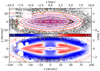 |
Fig. A.1. Mass-density MGE for FCC 153. Top: contours of the projected mass density (black), the mass density MGE∑ (red), and the surface brightness MGEμ (blue). Bottom: ratio between the mass and surface-brightness models, showing the structural differences. This panel is normalised by the average M⋆/L such that values of 1.0 (white) are consistent with the assumption of a spatially-constant M⋆/L, and any deviations are percentages in stellar mass. The outline of the MUSE mosaic is shown in dashed brown. |
MGE∑ for FCC 153.
Same as Table A.1, but for FCC 170.
Same as Table A.1, but for FCC 177.
Appendix B: Dynamical modelling
This section presents additional details of the Schwarzschild models and measured data products. The best-fit parameters of the Schwarzschild models are given in Table B.1, while their parameter-space distributions are shown in Figs. B.1–B.3. The measured (un-symmetrised) kinematics and stellar populations are presented in Figs. B.4–B.6. It can be seen that FCC 170 exhibits the highest degree of intrinsic triaxiality, with the lowest p, though the triaxiality is small in all cases. The intrinsic shapes recovered by our models are in good agreement with, for instance, those of the oblate galaxies of Jin et al. (2019). Interestingly, the dynamical model of the field S0 NGC 3115 (Poci et al. 2019) has larger intrinsic triaxiality than the three cluster S0 galaxies studied here, but this is likely a consequence of its higher stellar mass, and the more violent assembly history inferred for that galaxy.
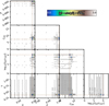 |
Fig. B.1. Optimisation over the 5D parameter-space for FCC 153. The grey points indicate the exploration of the parameter-space with the smaller orbit sampling, while the coloured points show the |

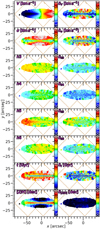 |
Fig. B.4. Un-symmetrised kinematics extracted for FCC 153 (left), and associated errors computed through Monte Carlo simulations (right). The outline of the MUSE mosaic is shown in dashed brown. |
Best-fit parameters for the Schwarzschild models.
Appendix C: Validation on mock data
A crucial test to conduct for the modelling procedure used in this work is to determine the accuracy and precision with which it can recover known properties. To this end, we conducted tests on mock data of realistic galaxies from the Auriga simulation suite (Grand et al. 2017). In Zhu et al. (2020), this Schwarzschild code is used to fit the mock kinematic data of sub-halos from Auriga, at various projected inclinations. Here we take the dynamical models and apply the procedure described in Sects. 3.3 and 3.4 in order to fit stellar populations in exactly the manner that is applied to the Fornax3D data. We then measure the diagnostics that inform the main scientific conclusions of this work, and compare directly to the underlying intrinsic distributions from the simulations. We conduct this analysis on Auriga halos 5 and 6, projected to an inclination of θ = 80°.
The stellar-population fits are shown in Fig. C.1, where the ‘true’ maps are generated simply by projecting all the particles along each LOS. We also ran 100 Monte Carlo simulation fits to these maps as is done in the main text, however in this case the outputs are less informative because the ‘errors’ on the mock maps were generated artificially. The distributions of t−z are presented in Fig. C.2. We note here that the ‘true’ distributions are smoother due to the ∼ 105 particles that are used to generate them, in contrast to the ∼ 102 dynamical components which constitute the ‘model’ distributions. Kernel Density Estimates (KDE) were computed from these data to compare the marginalised distributions. Owing to the difference in the size of the data sets between the dynamical models and simulations, we derived the optimal bandwidth for the KDE of each data-set using a data-driven approach which minimises the variance and also takes into account each sample size (Silverman 1986). This exercise has shown that not only can the models fit the projected maps, but also that our implementation recovers the underlying stellar-population distributions.
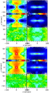 |
Fig. C.1. Stellar-population Schwarzschild model fits to the mock data. Mean stellar age (left) and metallicity (right) are shown for Auriga halos 5 (top) and 6 (bottom). From top to bottom: rows represent the true means, models fits, and residuals. |
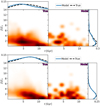 |
Fig. C.2. Intrinsic t−z distribution (left) and that retrieved from our model (right) for halos 5 (top) and 6 (bottom). The 1D distributions are also shown for each simulation, as kernel density estimates of the underlying data. The intrinsic distributions are black dashed curves, and the model distributions are the blue solid curves. |
The main results from this work are derived from the assembly histories in Figs. 10–12, and the AVR in Fig. 13. Comparing simulations to data in general can introduce inconsistencies in many ways, and so for clarity we describe the procedure for testing the recovery of the assembly histories on simulations, and the steps taken to mitigate potential inconsistencies. Firstly, the Cartesian coordinates of the simulation data are binned to the same spherical polar grid of the corresponding Schwarzschild model. The simulation kinematics, Vx, Vy, Vz, are then converted to cylindrical coordinates, in line with how the outputs from the Schwarzschild model are analysed. From here, the σz measurements on the simulation data proceed in an identical fashion as for the Schwarzschild model. Moreover, the distributions from the simulations are constructed using exactly the particles that lie within the mock FOV, by construction. Conversely, the Schwarzschild models (and indeed real observations) typically have contributions from orbits which reside (on average) outside the FOV, which are not present in the simulation. This means that any measurement on these data would be probing different physical regions between the two data sets. To remedy this inconsistency, the results from the Schwarzschild models do not include orbits with time-averaged radii outside the FOV. This is only the case for the mock tests where strictly-consistent comparisons are sought. Our main results in Figs. 10–12 include the full model.
The recovery of the assembly histories is presented in Fig. C.3. It can be seen that the radial profiles of σz from the simulations often extend to larger radii than the corresponding profiles from the Schwarzschild model. This is due to the fact that each particle in the simulation contributes to its profile, while for the Schwarzschild model orbits are required to have spent some time in a particular region before being included. A single particle (or very few) in the simulations of a given t − [Z/H] component may give the impression of having a larger extent compared to the Schwarzschild model, while actually contributing negligible mass. Therefore we emphasise that it is the common radial regions for each pair of profiles, and the overall spatial distribution of particles/orbits for each panel, that provides the best indication of the model’s recovery as this is where the vast majority of the mass resides. In this regime, there is clearly point-to-point variation between the intrinsic and recovered radial profiles of velocity dispersion, which are noisy for some components. The agreement is worse for decreasing mass, which is expected. Nevertheless, it can be seen that the general trends are accurately recovered by the model, in particular the relative dynamics between the different stellar populations. The absolute quantitative agreement between the model and simulations is also good, though in some cases there appears to be additional discretisation effects in the model producing sharply-varying profiles in the low-mass panels, which is likely due to the binning in circularity space combined with the binning in the t−z space. Reassuringly, the 2D distributions are also well-matched by the model. Some mass is re-distributed to different bins compared to the simulations, which are typically the compact spheroidal structures. Such ‘boundary’ effects are inevitable when imposing discrete binning on the data, as those components with values close to these boundaries may straddle one way or the other. The Monte Carlo simulations show similar behaviour, and in this way the shaded regions account for these boundary effects. Finally, the recovery of the AVR are shown in Fig. C.4. Once again, we see good qualitative and quantitative agreement.
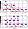 |
Fig. C.3. Similar to Fig. 10, showing the assembly history for halo 5 (top) and halo 6 (bottom). In addition to the σz radial profile (black/white line) and surface brightness distribution (upper right) from the Schwarzschild model, the shaded regions correspond to the variations derived from 100 Monte Carlo fits to the stellar population maps. Each panel also contains the intrinsic σz radial profile (red line) and surface brightness distribution (upper left) from the simulations. |
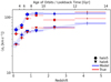 |
Fig. C.4. Similar to Fig. 13, showing the recovered (blue) and intrinsic (red) AVR for halos 5 and 6. |
We conclude that the model is sufficiently robust to be able to draw strong inferences about real galaxies. With regards to the main conclusions of this work, the relative behaviour of the chemo-dynamical populations is recovered well, where the model stellar AVR for both Auriga halos are consistent to within ∼ 10 km s−1 of their intrinsic values. We highlight that we believe this is an upper limit on account of our real data having higher spatial resolution, the corresponding models having higher orbit sampling, and all galaxies studied here having θ > 80° (where more edge-on projections are more reliable; Zhu et al. 2020), which all work in favour of improving the reliability of this technique further. We are therefore confident that this method is able to recover not only projected average quantities like the 2D stellar-population maps of Fig. C.1, but also quantitatively recover the underlying chemo-dynamic distributions, and that our main conclusions are robust against systematic effects.
All Tables
All Figures
|
Fig. 1. Fits (red) to spectra (black) from the centre and outer regions (top and bottom of each pair of spectra, respectively) for our galaxy sample, as labelled on the right. Residuals are shown in green, offset for presentation. The grey bands show regions which are masked during the fit. All spectra are normalised, but vertically offset for presentation. It can be seen that the outer spectra are more noisy, as expected, but that in all cases the data are reproduced well by the fit. |
| In the text | |
|
Fig. 2. Full r-band images from FDS, overlaid with the MUSE FOV in dashed brown for FCC 153 (left), FCC 170 (middle), and FCC 177 (right). |
| In the text | |
|
Fig. 3. Enclosed-mass profiles of the total (dynamical) mass (solid line), stellar mass (dashed line), and DM (dot-dashed line) for the three galaxies. The effective radii are denoted by the small arrows, and the radial extent of each spectroscopic FOV is shown by the vertical dotted line. The lower radial bound of the figure is set to half the width of the point-spread function from the spectroscopic observations. |
| In the text | |
|
Fig. 4. Phase-space of circularity λz as a function of cylindrical radius R for the best-fit model of FCC 153. The colour represents the orbital weight from the Schwarzschild model, which has been normalised to an integral of unity. The dynamical decomposition is overlaid in black, where only those components which have non-zero contribution to the original model are defined. The figure is shown on the radial extent of the spectroscopy for clarity, but the decomposition is conducted over the full Schwarzschild model. The black dashed line is the half-mass radius, derived from MGE∑, shown for scale. The distribution indicates the prevalence of high-angular-momentum (cold disk-like) co-rotating orbits in this galaxy, with very little contribution from hot (λz ∼ 0) or counter-rotating (λz < 0) orbits. |
| In the text | |
|
Fig. 5. Same as Fig. 4, but for FCC 170. This galaxy has a large contribution from hot central orbits, with most of the cold orbits appearing at larger radius. |
| In the text | |
|
Fig. 6. Same as Fig. 4, but for FCC 177. Similarly to FCC 153, this galaxy is dominated by co-rotating cold orbits. |
| In the text | |
|
Fig. 7. Best-fitting Schwarzschild model for FCC 153. The data (left), fits (middle), and residuals (right) of, from top to bottom, the dynamical model (surface brightness, velocity, velocity dispersion, and h3 − h6), and the subsequent stellar-population fitting (age and metallicity). The outline of the MUSE mosaic is shown in dashed brown. All residual panels show the absolute differences (data – model), but are offset such that green is zero. The stellar-population maps share a common colour-bar between galaxies for comparison. We note that for FCC 153, since the observed metallicity map reaches 0.4 dex along the major axis, and is itself an average through the LOS, we extend the upper bound for the individual components during the stellar-population fitting to 1.0 dex. |
| In the text | |
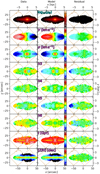 |
Fig. 8. Same as Fig. 7, but for FCC 170. |
| In the text | |
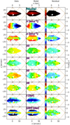 |
Fig. 9. Same as Fig. 7, but for FCC 177. |
| In the text | |
|
Fig. 10. Mass assembly history for FCC 153. The panels are ordered by increasing mean stellar age (left to right) and decreasing mean stellar metallicity (top to bottom). The value given at the top and right of each column and row, respectively, denotes its upper bound (inclusive). Each panel is composed of a radial profile of the vertical stellar velocity dispersion σz (black/white curve), the surface brightness distribution at the best-fitting projection (top-right) with the outline of the MUSE mosaic shown in dashed brown, and the total stellar mass within the FOV for that panel. The σz(R) profiles are coloured according to the stellar mass in that panel at that radius (sampled within the logarithmic radial bins). This indicates the spatial region in which each curve contributes most (white regions), and which regions may be impacted by numerical noise (black regions). The grey shaded regions show the spread of velocity dispersion profiles for 100 Monte Carlo fits to the stellar-population maps. This galaxy exhibits a dominant disk-like, metal-rich component that has steadily formed over the last ∼ 10 Gyr. |
| In the text | |
|
Fig. 11. Same as Fig. 10, but for FCC 170. This galaxy is dominated by an old central pressure-supported spheroidal component spanning ∼ 1 dex in metallicity. It has a secondary contribution from a progressively thinner and younger disk-like component, and a potential minor contribution from a warm metal-poor halo-like component. |
| In the text | |
|
Fig. 12. Same as Fig. 10, but for FCC 177. This galaxy appears to have begun forming late. It is dominated by a young, thin disk, with contributions from dynamically-warmer and slightly older stars. |
| In the text | |
|
Fig. 13. Stellar disk AVR as derived from our models. The coloured stars are the galaxies modelled in this work (and Poci et al. 2019, for NGC 3115). The symbol size is proportional to the fractional stellar mass in each age bin, for each galaxy independently. The horizontal error-bars denote the width of the age bin. The vertical error bars are computed as the weighted standard deviation within each age bin, for the best-fit model. The shaded regions show the spread in σz for 100 Monte Carlo fits to the stellar-population maps. The dashed curves show the stellar AVR of the four S0 galaxies when all orbits are included (no selection on orbital circularity). The box-whisker plots are literature measurements of cold gas disks, from HERACLES (Leroy et al. 2009), DYNAMO (Green et al. 2014), GHASP (Epinat et al. 2010), PHIBBS (Tacconi et al. 2013), MASSIV (Epinat et al. 2012), OSIRIS (Law et al. 2009), AMAZE-LSD (Gnerucci et al. 2011), SINS (Schreiber et al. 2009) and zC-SINF (Schreiber et al. 2014), KMOS3D (Wisnioski et al. 2015), and KDS (Turner et al. 2017). The black dots and crosses are Milky-Way stellar measurements (Yu & Liu 2018) for stars on (|z| < 270 pc) and off (|z| > 270 pc) the plane, respectively. Galaxy disks become dynamically colder towards the present day. The cluster S0 galaxies have a higher contribution from warmer orbits at more recent times compared to the field galaxy (comparing the full and disk-only σz). The Milky-Way, despite its higher stellar mass, is dynamically colder than the S0 galaxies studied here. |
| In the text | |
|
Fig. 14. Correlations of σz with stellar age at fixed metallicity (left), and stellar metallicity at fixed age (right) for, from top to bottom, the three galaxies studied in this work, and the field S0 NGC 3115 (Poci et al. 2019). The curves are coloured by their age/metallicity bin corresponding to those of Figs. 10–12. The Spearman rank coefficient r and the associated p-value, computed for all curves collectively in a given panel, are inset. The shaded regions correspond to the variations derived from 100 Monte Carlo fits to the stellar population maps. The stellar AVR at fixed metallicity exhibits lower significance than the [Z/H] − σz at fixed age. |
| In the text | |
|
Fig. A.1. Mass-density MGE for FCC 153. Top: contours of the projected mass density (black), the mass density MGE∑ (red), and the surface brightness MGEμ (blue). Bottom: ratio between the mass and surface-brightness models, showing the structural differences. This panel is normalised by the average M⋆/L such that values of 1.0 (white) are consistent with the assumption of a spatially-constant M⋆/L, and any deviations are percentages in stellar mass. The outline of the MUSE mosaic is shown in dashed brown. |
| In the text | |
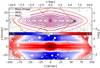 |
Fig. A.2. Same as Fig. A.1, but for FCC 170. |
| In the text | |
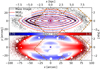 |
Fig. A.3. Same as Fig. A.1, but for FCC 177. |
| In the text | |
|
Fig. B.1. Optimisation over the 5D parameter-space for FCC 153. The grey points indicate the exploration of the parameter-space with the smaller orbit sampling, while the coloured points show the |
| In the text | |
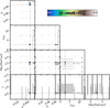 |
Fig. B.2. Same as Fig. B.1, but for FCC 170. |
| In the text | |
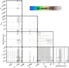 |
Fig. B.3. Same as Fig. B.1, but for FCC 177. |
| In the text | |
|
Fig. B.4. Un-symmetrised kinematics extracted for FCC 153 (left), and associated errors computed through Monte Carlo simulations (right). The outline of the MUSE mosaic is shown in dashed brown. |
| In the text | |
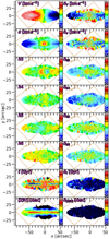 |
Fig. B.5. Same as Fig. B.4, but for FCC 170. |
| In the text | |
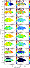 |
Fig. B.6. Same as Fig. B.4, but for FCC 177. |
| In the text | |
|
Fig. C.1. Stellar-population Schwarzschild model fits to the mock data. Mean stellar age (left) and metallicity (right) are shown for Auriga halos 5 (top) and 6 (bottom). From top to bottom: rows represent the true means, models fits, and residuals. |
| In the text | |
|
Fig. C.2. Intrinsic t−z distribution (left) and that retrieved from our model (right) for halos 5 (top) and 6 (bottom). The 1D distributions are also shown for each simulation, as kernel density estimates of the underlying data. The intrinsic distributions are black dashed curves, and the model distributions are the blue solid curves. |
| In the text | |
|
Fig. C.3. Similar to Fig. 10, showing the assembly history for halo 5 (top) and halo 6 (bottom). In addition to the σz radial profile (black/white line) and surface brightness distribution (upper right) from the Schwarzschild model, the shaded regions correspond to the variations derived from 100 Monte Carlo fits to the stellar population maps. Each panel also contains the intrinsic σz radial profile (red line) and surface brightness distribution (upper left) from the simulations. |
| In the text | |
|
Fig. C.4. Similar to Fig. 13, showing the recovered (blue) and intrinsic (red) AVR for halos 5 and 6. |
| In the text | |
Current usage metrics show cumulative count of Article Views (full-text article views including HTML views, PDF and ePub downloads, according to the available data) and Abstracts Views on Vision4Press platform.
Data correspond to usage on the plateform after 2015. The current usage metrics is available 48-96 hours after online publication and is updated daily on week days.
Initial download of the metrics may take a while.