| Issue |
A&A
Volume 646, February 2021
|
|
|---|---|---|
| Article Number | A38 | |
| Number of page(s) | 12 | |
| Section | Cosmology (including clusters of galaxies) | |
| DOI | https://doi.org/10.1051/0004-6361/202039075 | |
| Published online | 02 February 2021 | |
Very Large Array observations of the mini-halo and AGN feedback in the Phoenix cluster
1
Leiden Observatory, Leiden University, PO Box 9513, 2300 RA Leiden, The Netherlands
e-mail: This email address is being protected from spambots. You need JavaScript enabled to view it.
2
Kavli Institute for Astrophysics and Space Research, Massachusetts Institute of Technology, 77 Massachusetts Avenue, Cambridge, MA 02139, USA
3
DIFA, University of Bologna, Via Gobetti 93/2, 40129 Bologna, Italy
4
IRA INAF, Via Gobetti 101, 40129 Bologna, Italy
5
Department of Physics and Astronomy, University of Waterloo, Waterloo, ON, Canada
6
Département de Physique, Université de Montréal, C.P. 6128, Succ. Centre-Ville, Montréal, Québec H3C 3J7, Canada
Received:
31
July
2020
Accepted:
10
September
2020
Abstract
Context. The relaxed cool-core Phoenix cluster (SPT-CL J2344-4243) features an extremely strong cooling flow, as well as a mini halo. Strong star formation in the brightest cluster galaxy indicates that active galactic nucleus (AGN) feedback has been unable to inhibit this cooling flow.
Aims. We aim to study the strong cooling flow in the Phoenix cluster by determining the radio properties of the AGN and its lobes. In addition, we used spatially resolved radio observations to investigate the origin of the mini halo.
Methods. We present new multifrequency Very Large Array 1–12 GHz observations of the Phoenix cluster, which resolve the AGN and its lobes in all four frequency bands as well as the mini-halo in the L and S bands.
Results. Using our L-band observations, we measure the total flux density of the radio lobes at 1.5 GHz to be 7.6 ± 0.8 mJy, and the flux density of the mini halo to be 8.5 ± 0.9 mJy. Using high-resolution images in the L and X bands, we produced the first spectral index maps of the lobes from the AGN and find the spectral indices of the northern and southern lobes to be −1.35 ± 0.07 and −1.30 ± 0.12, respectively. Similarly, using L- and S-band data, we mapped the spectral index of the mini halo, and obtain an integrated spectral index of α = −0.95 ± 0.10.
Conclusions. We find that the mini halo is most likely formed by turbulent re-acceleration powered by sloshing in the cool core due to a recent merger. In addition, we find that the feedback in the Phoenix cluster is consistent with the picture that stronger cooling flows are to be expected for massive clusters such as this one, as these may feature an underweight supermassive black hole due to their merging history. Strong time variability of the AGN on Myr timescales may help explain the disconnection between the radio and the X-ray properties of the system. Finally, a small amount of jet precession of the AGN likely contributes to the relatively low intracluster medium re-heating efficiency of the mechanical feedback.
Key words: large-scale structure of Universe / radio continuum: galaxies / X-rays: galaxies: clusters / radiation mechanisms: non-thermal / galaxies: clusters: individual: SPT-CL J2344-4243
© R. Timmerman et al. 2021
 Open Access article, published by EDP Sciences, under the terms of the Creative Commons Attribution License (https://creativecommons.org/licenses/by/4.0), which permits unrestricted use, distribution, and reproduction in any medium, provided the original work is properly cited.
1. Introduction
The emission of strong X-ray radiation by the intracluster medium (ICM) in galaxy clusters suggests that this medium should often cool down rapidly: within a timescale of ∼109 years or fewer (e.g., Fabian 1994). As the ICM cools down, it is expected to flow down the gravitational well of the cluster, and accrete onto the galaxy at the center. This accretion of matter should then trigger star formation in the central galaxies proportionally to the cooling flow of the ICM. However, both this cooling of the ICM and the star formation in the center of the cluster are observed to be much weaker than expected (Fabian et al. 1982; McNamara & O’Connell 1989; Page et al. 2012; McDonald et al. 2018), leading to what is known as the “cooling flow problem”. The generally accepted solution to this problem is that feedback from active galactic nuclei (AGN) supplies energy to the ICM in the form of radiation and jetted outflows of plasma, thereby preventing the medium from cooling down (e.g., Brüggen & Kaiser 2002; McNamara & Nulsen 2007; Fabian 2012).
Studying this feedback process is essential to our understanding of the formation and evolution of galaxies, as it plays a critical role in the cooling of the ICM and the star formation in galaxies across cosmic time (e.g., Matteo et al. 2005; Croton et al. 2006; Menci et al. 2006; Sijacki et al. 2007; Lagos et al. 2008; Ciotti et al. 2010; Mathews & Guo 2011; Vogelsberger et al. 2014; Rasia et al. 2015). In particular, clusters of galaxies form a great opportunity to study AGN feedback, due to the relatively dense ICM, which is capable of creating strong cooling flows. The ICM is often also dense enough to keep the jetted outflows from the AGN contained, which allows this mechanical form of feedback to be studied in detail (McNamara & Nulsen 2012).
The interaction between the ICM and the jetted outflows from the AGN can be directly observed in the X-ray regime. As the jetted outflows displace the ICM, they create large cavities that are observed as depressions in X-ray observations. At radio frequencies, bubbles of synchrotron-emitting plasma are observed to be coincident with these cavities, verifying that these cavities are produced by the AGN (Gull & Northover 1973; Gitti et al. 2012).
Despite much research into AGN feedback in galaxy clusters, many open questions remain. Of particular interest for this work is the connection between the central AGN and the mini halo surrounding the brightest cluster galaxy (BCG). Mini halos are faint, diffuse synchrotron-emission regions commonly found in relaxed cool-core galaxy clusters. They span a region of a few hundred kpc, as they are generally confined to the cool-core region of a galaxy cluster. Mini halos often feature an amorphous shape, and have been found to show steep spectral indices of around α = −1 to α = −1.5 (Gitti et al. 2004; Giacintucci et al. 2019; Van Weeren et al. 2019).
The origin of mini halos remains a topic of debate, which is hampered by the difficulty of obtaining high-quality data on mini halos, as the central AGN often dominates the view. The emission of synchrotron radiation in the mini halo means that there must be a population of cosmic-ray electrons present in a magnetic field. However, based on the short lifetime of these electrons of 10–100 Myr, they must be accelerated in-situ (Brunetti & Jones 2014). Two mechanisms are proposed by which the electrons can be accelerated. In the hadronic model, relativistic, secondary electrons are injected by collisions between relativistic and thermal protons (e.g., Pfrommer & Enßlin 2004; Fujita et al. 2007). This model predicts the presence of diffuse gamma-ray emission, produced by the same proton-proton collisions and a gradual decrease in radio emission due to the diffusion of cosmic ray (CR) protons in the ICM. In the case of radio emission produced purely by secondary electrons, the spectral index would depend only on the energy distribution of the CR protons, and hence it would not vary with the radius.
Alternatively, according to the turbulent re-acceleration model, fossil electrons from the AGN are re-accelerated to high energies by magneto-hydrodynamic turbulence in the cluster (e.g., Gitti et al. 2002; Mazzotta & Giacintucci 2008; ZuHone et al. 2013). This turbulence is thought to generally be caused by strong cooling flows or a merger event in the recent history of the cluster, although recent observations of an Mpc-scale radio halo in a cool core cluster (Bonafede et al. 2014) and ultra-steep-spectrum emission extending beyond the cool core (Savini et al. 2018) have challenged that idea. The turbulent re-acceleration model predicts a possible steepening of the spectrum with radius and a radio brightness profile that is strongly contained by the cold fronts produced in the ICM by a recent merger event. These cold fronts are density discontinuities created by the cold and dense gas from the cool core or a subcluster moving through the surrounding hot gas, and therefore they also commonly form the boundary of a turbulent region (e.g., Markevitch & Vikhlinin 2007). Accurately determining the properties of mini halos is essential to understanding the underlying acceleration mechanism, and thereby their origin.
In this paper, we adopt a ΛCDM cosmology, with cosmological parameters of H0 = 70 km s−1 Mpc−1, Ωm = 0.3, and ΩΛ = 0.7. In this cosmology, the luminosity distance to the Phoenix cluster at z = 0.597 is 3508 Mpc, and an angular scale of 1 arcsecond at this redshift corresponds to 6.67 kpc. Furthermore, we followed the convention of defining our spectral indices according to S ∝ να.
2. The Phoenix cluster
In this work, we focus on the Phoenix cluster (SPT-CL J2344-4243), a massive galaxy cluster at redshift z = 0.597 discovered by Williamson et al. (2011) in the 2500 deg2 South Pole Telescope Survey. The Phoenix cluster is a relaxed cool-core cluster featuring a type 2 QSO (Ueda et al. 2013), and it is characterized by its high cooling flow and star formation rate (Kitayama et al. 2020). X-ray, optical, and infrared observations by McDonald et al. (2012, 2013, 2019) show a cooling flow of ∼3100 M⊙ per year, with a star-formation rate of ∼800 M⊙ yr−1. Whereas the star formation rate is generally on the order of 1% of the predicted cooling flow, for the Phoenix cluster this ratio is almost 30%, indicating that the feedback process has not been able to completely inhibit the cooling flow. Spectroscopic observations of the warm and cold gas in the core of the Phoenix cluster suggest that this rapid star formation may be a short phase, as the molecular gas supply is expected to deplete on a timescale of ∼30 Myr (McDonald et al. 2014).
Using Chandra observations, Hlavacek-Larrondo et al. (2014) revealed the presence of X-ray cavities in the ICM. Follow-up research using deeper observations by McDonald et al. (2015, 2019) provided an estimate of the scale of these cavities of 8–14 kpc, which suggests a jet power from the AGN of  erg s−1. In addition, star-forming filaments extending up to 50–100 kpc from the core of the cluster were observed using deep optical imaging. ALMA observations also show molecular gas filaments measuring 10–20 kpc in length tracing the edges of the X-ray cavities (Russell et al. 2017).
Observations using the Giant Metrewave Radio Telescope (GMRT) by Van Weeren et al. (2014) uncovered a mini halo surrounding the BCG, which spans a region of 400–500 kpc. This mini halo was later observed by Raja et al. (2020) using the Karl G. Jansky Very Large Array (VLA) in CnB configuration. By subtracting compact emission from their data, they detect the mini halo and derive a flux density of the mini halo at 1.5 GHz of 9.65 ± 0.97 mJy. They find that the 3σ contours of their map span a region of 310 kpc.
New deep Chandra and X-band VLA observations by McDonald et al. (2019) revealed radio jets that are coincident with the previously detected X-ray cavities. In addition, they present Hubble observations suggesting that the AGN may lift cool low-entropy gas up to larger radii, where it can cool faster than its fallback time, resulting in multiphase condensation. The gas kinematics and strong high-ionization emission lines indicate that relatively strong turbulence may be present in the core.
In this paper, we aim to investigate the strong cooling flow observed in the Phoenix cluster by imaging the AGN and its jetted outflows across a wide range of radio frequencies. In addition, we aim to study the origin of the mini halo by measuring its properties using spatially resolved radio observations for the first time.
3. Observations and data reduction
The Phoenix cluster was observed with the VLA in the L, S, C, and X bands, covering the frequency range from 1 GHz to 12 GHz (PI: McDonald, 17A-258). The X-band data of this project was previously presented by McDonald et al. (2019). In the L band, the VLA observed in both A and B configuration, which we complement with archival CnB-configuration observations (PI: Datta, 14B-397) recently presented by Raja et al. (2020). In the S, C, and X bands, the VLA observed in A, B, and C configuration. The L- and S-band observations were recorded using 16 spectral windows of 64 channels each, resulting in a total bandwidth of 1 GHz and 2 GHz, respectively. The C- and X-band observations were recorded using 32 spectral windows of 64 channels each, resulting in a total bandwidth of 4 GHz for both bands. All new observations have a total of 2.5 hours of integration time per configuration. An overview of the observations is presented in Table 1.
Summary of the observations.
For our new observations, we used 3C138 and 3C147 as primary calibrators with a total integration time of approximately five to ten minutes at the end of the observation. As the secondary calibrator, we used J0012-3954. Scans with an integration time of approximately two to three minutes on the secondary calibrator were repeated every 15 min. In the archival L band, CnB-array data, 3C48 was observed for 12 min as the primary calibrator. No secondary calibrator was included in this observation.
The data were reduced with the Common Astronomy Software Application (CASA; McMullin et al. 2007). The data reduction begins with a Hanning smoothing, the flagging of shadowed antennas, the calculation of gain elevation curves and corrections to the antenna positions, and the use of the TFCROP algorithm within CASA to apply automatic radio frequency interference (RFI) flagging. Next, manual flags were applied to exclude bad data from the calibration process. After the flagging, the initial complex gain solutions were calculated based on the central channels from each spectral window. These initial complex gain solutions were used to determine the delay terms. The bandpass calibration solutions were then derived based on the delay terms and the initial complex gain solutions. With the correct bandpass solutions applied, the complex gain solutions can be derived for the complete bandwidth of each spectral window. Using the polarized calibrator 3C138, we derived the global cross-hand delay solutions. The unpolarized calibrator, 3C147, then allowed the polarization leakage terms to be calculated. Finally, 3C138 was used again to calibrate the polarization angle. Using all relevant calibration tables, the complex gain solutions were redetermined, and the flux scale was set based on models of 3C138 and 3C147 by Perley & Butler (2013). The calibration solutions were then applied to the target source, after which the TFCROP and RFLAG automatic flagging algorithms were used to remove previously undetected RFI. Next, the calibrated data of the target source were split out, after which point the AOFLAGGER software (Offringa et al. 2010) was used to remove any remaining RFI.
Finally, we improved the calibration through the process of self-calibration. We used CASA to calculate new calibration solutions and applied these to the data, and we used WSCLEAN (Offringa et al. 2014) for the imaging and deconvolution. Each data set was self-calibrated by initially performing phase-only self-calibration, and later performing amplitude and phase self-calibration, with iteratively shorter calibration solutions. Then, all data sets of the same spectral band were concatenated to form one data set per band. These data sets were then self-calibrated again to obtain the final data sets. Imaging was performed using Briggs weighting (Briggs 1995) with a robust parameter of zero. The C-band data experienced issues during calibration, which is suspected to be caused by the very low declination of the source. For this reason, it is difficult to discern real structures from noise features near the AGN.
4. Results
The images we obtain are shown in Fig. 1. The L-band image shows the central compact AGN with the diffuse mini halo surrounding it. The mini halo is less visible in the S-band image due to its spectral slope, as well as the more compact beam. In the C-band image, the jetted outflows are visible toward the north and the south of the AGN. A small part of the mini halo is still visible toward the east and west of the AGN. Finally, the X-band image shows the jets at the highest angular resolution. The total flux densities, peak fluxes, root mean square (rms) noise levels, and beam sizes of the final images are summarized in Table 2.
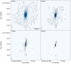 |
Fig. 1. VLA images of Phoenix cluster in L band (top-left), S band (top-right), C band (bottom-left), and X band (bottom-right). Contours are drawn at [ − 1, 1, 2, 4, 8, ...] × 4σrms, where σrms = 10.8 μJy beam−1 (L band), σrms = 5.9 μJy beam−1 (S band), σrms = 4.3 μJy beam−1 (C band), and σrms = 2.2 μJy beam−1 (X band). The beam sizes are indicated in the bottom-left corners of each panel. |
To show the maximum resolution attainable with each of the four data sets, images of the target using lower robust parameters are shown in Fig. 2. This shows that using a different weighting scheme, the jetted outflows can even be resolved in the L band. Comparing our observations to the ATCA observations of Akahori et al. (2020), we find that our VLA observations are able to resolve all components observed with the ATCA: C1 (AGN core), C2, C4, C5 (northern lobe), and C3 and C6 (southern lobe). Akahori et al. (2020) mention that they possibly detect jet precession, as components C3 and C4 (near the AGN), appear to be emitted in a different direction than components C2 and C6 in the northern and southern jets, respectively.
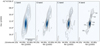 |
Fig. 2. VLA images of Phoenix cluster in L band (robust −1.5), S band (robust −1), C band (robust −0.5), and X band (robust 0). Contours are drawn at [ − 1, 1, 2, 4, 8, ...] × 4σrms, where σrms = 40.8 μJy beam−1 (L band), σrms = 12.8 μJy beam−1 (S band), σrms = 6.9 μJy beam−1 (C band), and σrms = 2.2 μJy beam−1 (X band). The source components as detected by Akahori et al. (2020) using the ATCA are indicated in the X-band map. The beam sizes are indicated in the bottom-left corners of each panel. |
The emission from the AGN appears to be coincident with the BCG, as shown in Fig. 3. In addition, the L-band emission extends far beyond the optical size of the BCG and the star-forming filaments. The radio emission from the cluster coincides with X-ray emission detected by Chandra (McDonald et al. 2015), as shown in Fig. 4. To confirm that the jetted outflows detected in our VLA observations are coincident with the cavities previously detected in the ICM, we subtracted a β-model from the X-ray map, and then overlaid the L- and X-band contours on the residuals, as shown in Fig. 5. Although there is a small subarcsecond uncertainty in the relative alignment between the images, it is clear that the X-ray cavities are inflated by magnetized radio plasma. We find no radio emission coincident with the possible ghost cavities previously marginally detected by McDonald et al. (2015) farther toward the north-east and south-east.
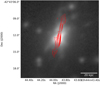 |
Fig. 3. Optical r-band image of Phoenix cluster taken with Megacam on the Magellan Clay Telescope (McDonald et al. 2015). The red contours indicate the X-band emission and are drawn at [ − 1, 1, 2, 4, 8, ...] × 4σrms, where σrms = 2.2 μJy beam−1. |
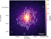 |
Fig. 4. X-ray (0.7–2 keV) image by Chandra (McDonald et al. 2015). The white contours indicate the L-band emission as observed with the Very Large Array and are drawn at [ − 1, 1, 2, 4, 8, ...] × 4σrms, where σrms = 10.8 μJy beam−1. |
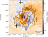 |
Fig. 5. Residuals of Chandra X-ray image (McDonald et al. 2015) minus a β-model. The residuals were smoothed by a boxcar function with a scale of three pixels (1.5 arcsec). The white contours indicate the emission in the X band as observed with the VLA and are drawn at [ − 1, 1, 4, 16] × 4σrms, where σrms = 2.2 μJy beam−1. The black contours indicate the emission in the L band as observed with the VLA, and are drawn at [ − 1, 1, 2, 4] × 4σrms, where σrms = 10.8 μJy beam−1. The black pluses indicate the positions of the ghost cavities detected by McDonald et al. (2015). |
To derive the overall spectral index of the source, we combined measurements of the total flux density of the cluster in our four bands with archival data from Mauch et al. (2003), McDonald et al. (2014), Van Weeren et al. (2014) and Akahori et al. (2020). We assume a 5% uncertainty on our flux density estimates in accordance with Perley & Butler (2017). By fitting a power-law profile through the data, we obtain an overall spectral index of −1.12 ± 0.02, as shown in Fig. 6. To account for a possible curvature in the spectrum, we fit a second-degree polynomial in log-space through the data, but find the curvature term to be consistent with zero within the 95% confidence interval. We excluded the data point at 220 GHz from this fit, as we expect that free-free and thermal dust emissions can significantly contribute to the spectrum at such high frequencies, causing the model of a single power law to break down.
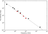 |
Fig. 6. Spectral energy distribution of Phoenix cluster. The black dots show data obtained from literature. The red dots show data presented in this work. The best-fit spectral index through the data is −1.12 ± 0.02. A curvature term is included in the fit, but is found to be negligible. The data point at 220 GHz is excluded from the fit as free-free and thermal dust emissions are expected to contribute significantly at this frequency. |
To study the mini halo and the AGN, we needed to separate these two components. By producing a map of the source using only the long baselines, we obtained an image of the AGN and its jets, without contamination from the more extended mini halo. Based on the X-band imaging, we find that the AGN and its jets are more compact than an angular scale of ten arcseconds, which corresponds to a limit on the baseline length of 20 kλ. After having produced an L-band image using only baselines longer than 20 kλ, we find that the remaining flux density of the source is 25.2 mJy within the 3σ contours. Comparing this flux density to the total flux density of 33.8 mJy, we find that there is a discrepancy of 8.6 mJy, which we attribute to the mini halo.
Alternatively, the flux density of the mini halo can be estimated through radial profile fitting by describing both the AGN and the mini halo using circular Gaussians. This enables the flux of the AGN and the mini halo to be spatially disentangled, thereby potentially providing a more accurate measurement of their total flux densities. We produced an L-band image with a Briggs robust parameter of −1 to improve the resolution of the image, and thereby reduced the scale of the central AGN. This image was smoothed to a circular beam of 2.8 arcseconds based on the major axis of the image. Through a least-squares fitting, we obtained separate estimates for the flux density of the AGN and the mini halo. For the AGN, we find a flux density of 23.6 ± 2.4 mJy, whereas we find a flux density of 8.5 ± 0.9 mJy for the mini halo.
Similarly, we can perform a radial fit with all compact emission masked out, as we know that the jetted outflows are only present in the northern and southern directions, which can cause a systematic error. With the L-band map produced using only long baselines, we were able to define a mask of where we expected the source to be dominated by compact structure. Outside of this mask, the mini halo is expected to be the dominant component. We defined this mask as the 3σ region in the 20 kλL-band map. Using this mask, we were able to fit the source using a single Gaussian profile to represent the mini halo. The estimate obtained with a mask for the flux density of the mini-halo is considerably lower, at only 5.9 mJy. As the values obtained from the first two methods agree very well, we adopt a value of 8.5 mJy for the flux density of the mini halo in L band for the rest of this paper.
From the radial fitting process, we can also obtain an estimate for the extent of the mini halo. From the radial fit, we find that it can be described by a Gaussian with a FWHM of 13.8 arcseconds, deconvolved with the beam. At a redshift of z = 0.597, this corresponds to a scale of 92 kpc. The maximum observable radius of the mini halo – defined as the radius at which the mini halo reaches the noise level – is 17.8 arseconds, or about 120 kpc. This gives a total diameter of the mini halo of ∼240 kpc.
To map the spectral index of the halo, we smoothed both the L-band and the S-band images to a circular beam size of five arcseconds and aligned the images by matching the positions of a nearby point source. To avoid contamination from the AGN and its jets, we masked out the central region using the same mask as with the radial fitting. After calculating the spectral index between the two maps and excluding the masked region, we obtained the spectral index map of the mini halo as shown in Fig. 7.
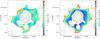 |
Fig. 7. Left: spectral index map from L- and S-band images. Right: corresponding uncertainties of the spectral index map. The contours show the L-band image smoothed to a resolution of five arcseconds and are drawn at [ − 1, 1, 2, 4, 8, ...] × 4σrms, where σrms = 17.9 μJy beam−1. The circular beam of five arcseconds is shown in the bottom-left corner. |
The spectral index map of the mini halo shows an annulus with a mean spectral index of α = −0.95 ± 0.10. However, the signal-to-noise ratio is too low to provide insight about any potential gradients or cut-offs in the spectrum as a function of radius. Using this spectral index, we calculated the radio luminosity of the mini halo using
 (1)
(1)
where S1.4 GHz is the flux density at 1.4 GHz and DL is the luminosity distance to the source, and we find a value of P1.4 GHz = (13.0 ± 1.4) × 1024 W Hz−1.
To map the spectral index of the AGN and its lobes, we took the high-resolution L-band image, as shown in Fig. 2, and we smoothed the X-band image to this resolution. Next, we aligned the images based on a nearby point source. By calculating the spectral index between the L band and X band, we obtain the map shown in Fig. 8.
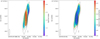 |
Fig. 8. Left: spectral index map from L- and X-band images. Right: corresponding uncertainties of the spectral index map. The contours show the X-band image smoothed to the L-band resolution and they are drawn at [ − 1, 1, 2, 4, 8, ...]× 4σrms, where σrms = 2.6 μJy beam−1. The beam is shown in the bottom-left corner. |
In this spectral index map, we can resolve both the spectral indices of the two lobes, as well as the spectral index of the AGN. We find that the northern lobe has a spectral index between the L and X bands of −1.35 ± 0.07, and the southern lobe has a spectral index of −1.30 ± 0.12. The AGN in the center of the map shows a spectral index of −0.86 ± 0.04. Due to the alignment of the lobes with the synthesized beam, we do not have the resolution required to check for a spectral gradient along the outflows. By subtracting a point source convolved with the beam from the high-resolution L-band image, we find that the radio lobes have a total flux density of 7.6 ± 0.8 mJy.
Finally, as we have VLA observations in full polarization mode, we checked for polarized emission using RM synthesis. However, we were unable to find a significant amount of polarized emission from the cluster, which is consistent with the results of Akahori et al. (2020).
5. Discussion
5.1. The origin of the mini halo
Our VLA observations clearly resolve the mini halo and the AGN in the Phoenix cluster. We estimate the mini halo to have a maximum observable deconvolved diameter of about 240 kpc, and a radio luminosity at 1.4 GHz of P1.4 GHz = (13.0 ± 1.4) × 1024 W Hz−1. Our estimate for the size of the mini halo is smaller than that of Van Weeren et al. (2014), who estimated a size in the range of 400–500 kpc using 610 MHz GMRT observations. This may be an indication of spectral steepening in the outer regions of the mini halo, as a detection by the GMRT at 610 MHz and a non-detection by the VLA at 1.5 GHz in this region implies a spectral index steeper than α = −1.5, based on the rms noise levels in both maps. However, we do not see a trend in our spectral index maps to suggest such a spectral steepening. In addition, the GMRT data suffers from a relatively poor angular resolution and sensitivity compared to the VLA, so we cannot make any definite claims on the spectrum of the mini halo in the outer regions. Our reported value for the radio luminosity at 1.4 GHz is consistent with previous estimates by Van Weeren et al. (2014) and Raja et al. (2020), who calculated values of P1.4 GHz = (10.4 ± 3.5) × 1024 W Hz−1 and P1.4 GHz = (14.38 ± 1.80) × 1024 W Hz−1, respectively.
We mapped the spectral index of the mini halo and derive an integrated spectral index between the L and S bands of −0.95 ± 0.10, which is consistent with the spectral index of −0.98 ± 0.16 as derived by Raja et al. (2020) between 610 MHz and 1.5 GHz. We were unable to find evidence for a radial gradient in the spectral index map due to the low signal-to-noise ratio.
Further insight into the origin of the diffuse emission can be provided by the spatial correlation between the radio (IR) and X-ray (IX) surface brightnesses. This correlation is expected because the relativistic electron population, and hence the radio emission, are predicted to be linked to the thermal plasma in both hadronic and re-acceleration models. The IR–IX correlation allows us to constrain the distribution of the nonthermal ICM components with respect to the thermal plasma and thereby investigate the origin of the radio emission (e.g., Brunetti & Jones 2014; Ignesti et al. 2020).
We used the Monte Carlo point-to-point analysis presented in Ignesti et al. (2020) to evaluate the IR–IX correlation for the Phoenix cluster. We use a circularly smoothed image of the Phoenix cluster in the L band with a Briggs robust parameter of −1 to improve the resolution of the map, and thereby reduce the area affected by AGN-related emission while simultaneously increasing the amount of samples of mini-halo emission. The X-ray surface brightness is obtained from archival Chandra observations. The surface brightnesses IR and IX have been sampled with 1000 randomly-generated meshes. For the cells in the mini-halo region, values of IR and IX are measured and fit with a power-law relation,  , using the BCES algorithm (Akritas & Bershady 1996). We present in Fig. 9 both the result of the analysis performed on a single grid (left panel) and the final result of the MC routine (right panel). We measured a sub-linear scaling index, k, of 0.84 ± 0.23, which indicates that the radio emission likely declines slower than the X-ray emission. This result is interestingly more similar to what is observed for giant radio halos – which often feature sub-linear indices k in the range of 0.5 to 1.0 (Govoni et al. 2001; Feretti et al. 2001; Giacintucci et al. 2005; Hoang et al. 2019; Xie et al. 2020) – than to mini halos, which generally feature a super-linear scaling with indices k in the range of 1.1 to 1.3 (Ignesti et al. 2020). Such a flat index, k, indicates that the X-ray emission is more peaked than the radio emission, which is in agreement with the exceptionally luminous cool core of this cluster. Therefore, it suggests that the distribution of nonthermal components does not strongly depend on the properties of the cool core.
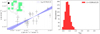 |
Fig. 9. Results from Monte Carlo point-to-point analysis. Left: an example of an estimate for k using a particular choice for the grid position. The data points and error bars show the estimated radio surface brightness vs. X-ray surface brightness for a given grid cell. The slope of the best-fit power law through these data (blue line) is shown in the legend. The contours in the top-left corner indicate the [3,6,12,24,48] × σ contours of the circularly-smoothed L-band image with a Briggs robust parameter of −1, where σ = 18 μJy. The beam size is 2.8 arcseconds circular, and is indicated by the solid black circle. Right: histogram of all values of k from the Monte Carlo point-to-point analysis. The resulting best estimate for kMC is reported in the legend. |
On the basis of these results, we can explore the scenario of purely hadronic origin of relativistic electrons. We followed the approach presented in Ignesti et al. (2020) to infer the ICM magnetic field to constrain the physical boundaries of the hadronic model for the Phoenix cluster. We used the thermodynamic profiles from McDonald et al. (2015) to compute the ICM electron density and temperature. From these, we numerically calculated the X-ray emissivity. Assuming a hadronic model, we can compare these to the radio emissivity expected in a pure hadronic model (e.g., Brunetti et al. 2012) to constrain the magnetic field configurations that are consistent with our value of the index k. We assume a magnetic field profile of the form
 (2)
(2)
where B0 and n0 are the central values of the magnetic field strength and the thermal ICM number density, respectively, and the index η determines the scaling relation between the magnetic field and the ICM density. The constraints we derive on the magnetic field configuration are shown in Fig. 10. We find that for typical values of the central magnetic field strength (10–20 μG; Carilli & Taylor 2002), we require the index η to be 0.2–0.3, indicating that the ICM density is much more peaked than the magnetic field strength. Similarly, for a typical value of η = 0.5, we require the central magnetic field strength to be at least 50 μG, which is far higher than commonly observed.
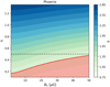 |
Fig. 10. Index k for combinations of magnetic field strength and the index η. The horizontal dashed line at η = 0.5 indicates the equilibrium configuration between thermal and nonthermal energy density. The red region indicates the parameter space consistent with values of k that we obtained using the Monte Carlo point-to-point analysis. |
To provide context to these estimates of the magnetic field configuration from the point-to-point analysis, we also calculate the equipartition magnetic field. Under the assumption that the magnetic field and the cosmic ray particles evolve over similar timescales, they are expected to be coupled. This coupling is supposed to lead to an equilibrium between the energy densities of the cosmic ray particles and the magnetic field (Govoni & Feretti 2004; Beck & Krause 2005). For the classical equipartition magnetic field, we obtain a field strength of 3.4 μGauss. For the revised equipartition magnetic field, we obtain a field strength of 5.5 μGauss using a commonly adopted value of γmin = 100 for the low-energy cut-off of the cosmic ray particle energy distribution. This shows that the equipartition magnetic field strength is much lower than the magnetic field strength predicted by a hadronic model.
In addition, we can test predictions from hadronic models on the spectral index of the mini-halo. According to a hadronic model, the radio-emitting electrons are injected by collisions between cosmic-ray protons from the AGN and thermal protons in the ICM. This implies that the synchrotron spectral index α is directly proportional to the cosmic ray proton injection spectral index δ as α ≈ δ/2 (e.g., Blasi & Colafrancesco 1999; Pfrommer & Enßlin 2004; Brunetti et al. 2017). Therefore, our spectral index of α = −0.95 ± 0.10 requires a cosmic ray proton injection spectral index of δ = −1.90 ± 0.20, but such a flat distribution is only marginally consistent with the generally observed values of δ in the range of −2.1 to −2.4 (e.g., Völk et al. 1996; Blasi & Colafrancesco 1999; Schlickeiser 2002; Enßlin 2003; Pinzke & Pfrommer 2010).
As we find that both the magnetic field configurations obtained by assuming a hadronic model and the relatively flat spectral index of the mini halo are inconsistent with the values generally reported in literature, we conclude that our results disfavor a pure hadronic origin of the radio emission, although we cannot exclude that proton-proton collisions played a role in the origin of seed electrons for the re-acceleration. Therefore, a turbulent re-acceleration model is the preferred model to explain the origin of the mini halo in the Phoenix cluster. However, the question remains as to what causes this turbulence.
Mazzotta & Giacintucci (2008) observed a correlation between the mini-halo emission and the spiral-shaped cold fronts produced by sloshing of the gas in the cool core (Markevitch et al. 2003; Ascasibar & Markevitch 2006). Magneto-hydrodynamic simulations by ZuHone et al. (2011a,b, 2013, 2015) show that this sloshing can induce turbulence and amplify the magnetic fields required to re-accelerate thermal electrons to relativistic speeds. In addition, their simulations predict luminosities and spectral indices that are in agreement with observations. Recent research by Richard-Laferrière et al. (2020) suggests that in addition to sloshing, AGN feedback may also contribute significantly to the amount of turbulence. For the Phoenix cluster, we find that the extent of the mini halo matches with the extent of the sloshing pattern in the ICM observed using X-ray data (see Fig. 5). Toward the south of the AGN, the mini halo appears to be confined to the overdense region in the ICM, whereas toward the west it appears to be confined to the underdense region in the ICM.
On the other hand, Gitti et al. (2002, 2004, 2007) suggested that the turbulence in the core can be induced by the strong cooling flow accreting onto the cool core. If so, a direct relation is expected between the mini-halo cooling flow power Pcf and the integrated mini-halo radio power νPMH. The cooling flow power is calculated as Pcf = ṀkT/μmH, where Ṁ is the mass accretion rate, k is Boltzmann’s constant, T is the temperature of the ICM, μ is the mean molecular weight, and mH is the mass of a hydrogen atom. We plotted the correlation between these two properties based on the Giacintucci et al. (2019) sample of mini halos, as shown in Fig. 11. As previously verified by Doria et al. (2012) and Bravi et al. (2015) using different samples, this correlation between the cooling flow power and the integrated radio power of the mini halo is indeed present. However, the relatively large intrinsic scatter suggests that this correlation may not indicate a causal connection between the cooling flow rate and turbulence in the cool core. Instead, this correlation could, for example, emerge due to dependence on a third parameter.
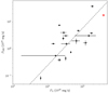 |
Fig. 11. Cooling flow power versus mini-halo radio luminosity at 1.4 GHz for the sample of mini halos from Giacintucci et al. (2019). The red data point indicates the Phoenix cluster. The dashed grey line indicates the best power-law fit through the data and is given by log PMH[1040 erg s−1] = (1.37 ± 0.17)log Pcf[1040 erg s−1]−(6.07 ± 0.79). The integrated mini-halo luminosities are from Giacintucci et al. (2019) and this work. Values of the cooling rates and ICM temperatures are from Arnaud et al. (1987), Churazov et al. (2003), Gitti & Schindler (2004), Böhringer et al. (2005), Covone et al. (2006), Leccardi & Molendi (2008), Bravi et al. (2015), McDonald et al. (2015, 2018), Main et al. (2016), and Werner et al. (2016). |
Therefore, we conclude that the turbulent re-acceleration model powered by sloshing is the prime candidate to explain the origin of the mini halo. Based on the close similarities between the mini-halo emission region and the sloshing region, and the agreement between the observed spectral index and theoretical predictions, we find sloshing to be the main source of turbulence in the ICM, although we do not exclude that the exceptionally strong cooling flow in the Phoenix cluster may have partly contributed to the turbulence.
5.2. The extreme feedback in the Phoenix cluster
Two of the main open questions about the feedback process in the Phoenix cluster remain: why does this cluster feature such a strong cooling flow and why are the radio and X-ray observations so disconnected. According to the explanation recently proposed by McDonald et al. (2018), the strong cooling flow could be a consequence of the way the most massive clusters (such as the Phoenix cluster) are formed. As lighter clusters merge and form more massive clusters, their low-entropy gas content merge relatively quickly compared to their central galaxies. This delayed merging of the central galaxies leads to the most massive clusters having relatively underweight supermassive black holes powering their AGNs, as they generally have a rich and recent merging history. For supermassive black holes, it has been observed that the mechanical power levels off as the accretion rate reaches a few percent of the Eddington rate (Russell et al. 2013). This is in contrast to the radiative power of the AGN, which continues to increase with the accretion rate. In the context of a galaxy cluster, this means that if the central supermassive black hole is underweight, the same accretion rate of the AGN is more likely to reach this saturation point and result in the AGN being unable to compensate for the cooling flow with mechanical feedback. Verifying this explanation would require precise measurements of the black hole masses, which we cannot derive from our radio observations. Therefore, definitively answering this open question is not the goal of this work. However, we can investigate if our observations are consistent with this explanation.
According to this explanation, the overall feedback process in the Phoenix cluster is not abnormal. Instead, the Phoenix cluster should simply be in the tail of the distribution. To see in which aspects the Phoenix cluster is an outlier to the general population, we looked into its cavity power and ICM cooling rate. The cavity power Pcav of a cluster can be estimated by dividing the total enthalpy Ecav of the cavities by the buoyant rise time. Here, the total enthalpy Ecav can be calculated as Ecav = 4 PV, where P is the total pressure of the ICM at the position of the cavities and V is the volume of the cavities. The buoyant rise time is the time required for the cavities to move from the AGN to their present position under the assumption that they rise through the ICM buoyantly. The ICM cooling rate within a particular radius indicates how much mass in the ICM cools down per year due to the emission of thermal bremsstrahlung, and it can be calculated as the ICM mass enclosed within the given radius divided by the cooling time. We plotted the cavity power versus the ICM cooling rate for the Phoenix cluster and the sample of clusters from Rafferty et al. (2006), as shown in Fig. 12. Here we find that the Phoenix cluster is the most extreme cluster in the sample, both in terms of the cooling flow rate and the cavity power. However, the Phoenix cluster is consistent with the observed correlation. Similarly, we plotted the radio luminosity of the jetted outflows at 1.4 GHz, as well as the bolometric radio luminosity, against the cavity power, for a sample of clusters, as shown in Fig. 13. This is where the Phoenix cluster does appear to be an outlier, as the cavity power is too high for both the bolometric radio luminosity of the lobes and their radio luminosity at 1.4 GHz. This is amplified if we plot the cooling flow rate against the bolometric radio luminosity of the lobes, as shown in Fig. 14. In this comparison, the Phoenix cluster is a strong outlier in the correlation. For its cooling flow rate, the radio lobes in the Phoenix cluster are far too faint.
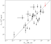 |
Fig. 12. ICM cooling rate Ṁcool vs. cavity power Pcav for the sample of clusters from Rafferty et al. (2006). The red data point indicates the Phoenix cluster. The gray dashed line indicates the best power-law fit through the data and is given by log Pcav[1042 erg s−1] = (1.00 ± 0.10) log Ṁcool[M⊙/yr] + (0.45 ± 0.24). All black data points are from Rafferty et al. (2006) and McDonald et al. (2018), and the Phoenix cluster data are from McDonald et al. (2015, 2019). |
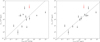 |
Fig. 13. Left: radio luminosity of the lobes at 1.4 GHz vs. cavity power for Phoenix cluster (red) and the Bîrzan et al. (2008) sample of mini halos (black). The dashed line shows the best power-law fit through the data and is given by log Pcav[1042 erg s−1] = (0.86 ± 0.20)log P1400[1024 W Hz−1]+(1.63 ± 0.29). Right: bolometric radio luminosities of the lobes between 10 MHz and 10 GHz for the same sample. The dashed line shows the best power-law fit through the data and is given by log Pcav[1042 erg s−1] = (0.79 ± 0.15) log Lradio[1042 erg s−1]+(2.03 ± 0.19). Phoenix cluster data are from McDonald et al. (2019) and this work, and data for the other clusters are from Bîrzan et al. (2008). |
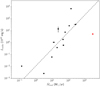 |
Fig. 14. ICM cooling rate Ṁcool vs. bolometric radio luminosity of lobes between 10 MHz and 10 GHz. The red data point indicates the Phoenix cluster, and the black data points indicate the sample of Bîrzan et al. (2008). The dashed line shows the best power-law fit through the data and is given by log Lradio[1042erg s−1] = (1.41 ± 0.35) log Ṁcool[M⊙/yr] − (1.95 ± 0.53). Phoenix cluster data are from McDonald et al. (2019) and this work, and data for the other clusters are from Bîrzan et al. (2008), McDonald et al. (2019). |
We observe a disconnection between the radio- and the X-ray properties of the Phoenix cluster. In the radio regime, the AGN in the Phoenix cluster appears to be relatively modest, whereas in the X-ray regime, both the AGN and the cooling flow are among the strongest of all known clusters. We suspect that this difference between the radio and the X-ray may be caused by strong time variability of the AGN on Myr timescales. In our radio observations, both the northern and southern lobes appear to be detached from the AGN, and this feature is also visible in the ATCA observations presented by Akahori et al. (2020). In addition, we find that the central AGN is not a perfect point source, but it is elongated toward the northwest and southeast, indicating that new outflows are being detected. Outburst power has been observed to vary from factors of several in Hydra A (Wise et al. 2007) to two orders of magnitude in MS0735 (Vantyghem et al. 2014) over timescales of tens of Myr. This observed variability has been corroborated by numerical simulations (e.g., Li et al. 2015; Prasad et al. 2015), providing an explanation for the lobe structure in the Phoenix cluster. It is possible that the sloshing in the ICM contributes in part to this AGN variability by displacing the accretion material of the AGN, similar to as observed in A2495 by Pasini et al. (2019). However, whereas the BCG in A2495 appears to be oscillating back and forth through the cool core, the BCG in the Phoenix cluster is stationary at the center of the cool core. This means that sloshing can only affect the AGN activity if it inhibits the cooling flow. Detailed simulations by Zuhone et al. (2010) suggest that sloshing mainly introduces variability in the cooling flow on timescales of 1 Gyr or more. These timescales are too long to explain the AGN variability in the Phoenix cluster, so we consider it to be unlikely that sloshing plays a major role. In this scenario, the lack of radio luminosity would be caused by a break in the AGN activity, as the only contribution to the lobe radio luminosity is caused by a relatively short and old outburst. This break in the AGN activity would not necessarily affect the currently observed cavity power, as the cavities require time to expand, and they are therefore more dependent on a later stage of an outburst. However, the current volume of the cavities will not be sustainable due to this AGN variability. As the break in the outflows reaches the cavities, they will deflate, resulting in the average cavity power likely being lower than the presently observed value.
Finally, the relatively low amount of jet precession observed in the Phoenix cluster by Akahori et al. (2020) and our X-band observations likely also contributes to the low ICM re-heating efficiency of the mechanical feedback, as the energy from the AGN is not distributed isotropically, but rather predominantly in the direction of the jets. The explanation by McDonald et al. (2018) combined with time variability of the AGN activity and a low jet precession angle may resolve some of the remaining open questions on the AGN feedback in the Phoenix cluster, although a more quantitative investigation would be required to confirm the validity of this model.
6. Conclusions
In this paper, we present new Karl G. Jansky Very Large Array observations, enabling the radio lobes of the AGN and the mini halo in the Phoenix cluster to be studied in detail at frequencies from 1 to 12 GHz. In particular, our observations resolve the radio lobes of the AGN in all four frequency bands, and the mini halo can be detected in both our L and S bands. Using these multifrequency observations, we studied the remarkable feedback scenario in the Phoenix cluster and the origin of its mini halo.
We find that the total flux density of the source at 1.5 GHz is 33.8 ± 1.7 mJy, with an overall spectral index of −1.12 ± 0.02. Using our L- and S-band observations, we find that the mini halo has an average spectral index of −0.95 ± 0.10. By subtracting compact emission and through radial profile fitting, we find that the mini halo has a total flux density at 1.5 GHz of 8.5 ± 0.9 mJy, which corresponds to a radio luminosity at 1.4 GHz of (13.0 ± 1.4) × 1024 W Hz−1. In addition, we find that the mini halo has a maximum observable radius in the L band of 240 kpc. At 1.5 GHz, the radio lobes show a total flux density of 7.6 ± 0.8 mJy, and spectral indices with respect to 10 GHz of −1.35 ± 0.07 (northern lobe) and −1.30 ± 0.12 (southern lobe).
Due to the relatively flat spectral index of the mini halo, the low index k, and the extreme magnetic field configuration we obtain by assuming a hadronic model, we conclude that our results disfavor a pure hadronic origin of the mini halo. On the contrary, we confirm the correlation between the cooling flow power and the radio luminosity of the mini halo with respect to other clusters. Also, we observe the sloshing pattern in the ICM to match with the extent of the mini halo at radio frequencies, and we find our integrated spectral index of the mini halo to be consistent with numerical predictions for a turbulent re-acceleration model. For these reasons, we conclude that a turbulent re-acceleration model is the preferred model to explain the origin of the mini halo, and in particular we favor sloshing in the cool-core as an explanation for the turbulence.
By measuring the flux density of the radio lobes in the L band for the first time, the mechanical feedback in the Phoenix cluster has been studied from a radio perspective. We observe a disconnection between the X-ray and radio properties of the Phoenix cluster: the cavity power and cooling flow rate are both among the most extreme ever measured, whereas the bolometric radio luminosity of the lobes is relatively modest. We find that the feedback in the Phoenix cluster is overall consistent with the proposed explanation by McDonald et al. (2018), which states that the strong cooling rate and inefficient feedback are characteristic of more massive clusters. Strong time variability of the AGN activity on Myr timescales may explain the disconnection between the radio and the X-ray properties of the system. Finally, a small amount of jet precession likely also contributes to the low ICM re-heating efficiency of the AGN feedback.
For future research, it would be valuable to obtain more high-resolution radio observations of a sample of mini halos to further test the correlation between the mini-halo emission and the sloshing pattern in the ICM, as this could provide very strong evidence for the turbulent re-acceleration model, and current results look promising. In addition, low-frequency observations may test whether the sloshing of the ICM produces more extended, ultra-steep spectrum emission beyond the cold fronts, as observed in the cases of PSZ1G139.61+24 and RXJ1720.1+2638 by Savini et al. (2018, 2019).
Acknowledgments
We would like to thank the anonymous referee for useful comments. RT and RJvW acknowledge support from the ERC Starting Grant ClusterWeb 804208. Support for this work was provided to MM by NASA through Chandra Award Number GO7-18124 issued by the Chandra X-ray Observatory Center, which is operated by the Smithsonian Astrophysical Observatory for and on behalf of the National Aeronautics Space Administration under contract NAS8-03060.
References
- Akahori, T., Kitayama, T., Ueda, S., et al. 2020, PASJ, 72, 62 [CrossRef] [Google Scholar]
- Akritas, M. G., & Bershady, M. A. 1996, ApJ, 470, 706 [NASA ADS] [CrossRef] [Google Scholar]
- Arnaud, K. A., Johnstone, R. M., Fabian, A. C., et al. 1987, MNRAS, 227, 241 [NASA ADS] [Google Scholar]
- Ascasibar, Y., & Markevitch, M. 2006, ApJ, 650, 102 [NASA ADS] [CrossRef] [Google Scholar]
- Beck, R., & Krause, M. 2005, Astron. Nachr., 326, 414 [NASA ADS] [CrossRef] [Google Scholar]
- Böhringer, H., Burwitz, V., Zhang, Y. Y., et al. 2005, ApJ, 633, 148 [NASA ADS] [CrossRef] [Google Scholar]
- Bîrzan, L., McNamara, B. R., Nulsen, P. E. J., et al. 2008, ApJ, 686, 859 [NASA ADS] [CrossRef] [Google Scholar]
- Blasi, P., & Colafrancesco, S. 1999, Astropart. Phys., 12, 169 [NASA ADS] [CrossRef] [Google Scholar]
- Bonafede, A., Intema, H. T., Brüggen, M., et al. 2014, MNRAS, 444, L44 [NASA ADS] [CrossRef] [Google Scholar]
- Bravi, L., Gitti, M., & Brunetti, G. 2015, MNRAS, 455, L41 [NASA ADS] [CrossRef] [Google Scholar]
- Briggs, D. S. 1995, PhD Thesis, New Mexico Institude of Mining and Technology [Google Scholar]
- Brüggen, M., & Kaiser, C. R. 2002, Nature, 418, 301 [NASA ADS] [CrossRef] [PubMed] [Google Scholar]
- Brunetti, G., & Jones, T. W. 2014, Int. J. Mod. Phys. D, 23, 1430007 [Google Scholar]
- Brunetti, G., Blasi, P., Reimer, O., et al. 2012, MNRAS, 426, 956 [NASA ADS] [CrossRef] [Google Scholar]
- Brunetti, G., Zimmer, S., & Zandanel, F. 2017, MNRAS, 472, 1506 [NASA ADS] [CrossRef] [Google Scholar]
- Carilli, C. L., & Taylor, G. B. 2002, ARA&A, 40, 319 [NASA ADS] [CrossRef] [Google Scholar]
- Churazov, E., Forman, W., Jones, C., & Böhringer, H. 2003, ApJ, 590, 225 [NASA ADS] [CrossRef] [Google Scholar]
- Ciotti, L., Ostriker, J. P., & Proga, D. 2010, ApJ, 717, 708 [NASA ADS] [CrossRef] [Google Scholar]
- Covone, G., Adami, C., Durret, F., et al. 2006, A&A, 460, 381 [NASA ADS] [CrossRef] [EDP Sciences] [Google Scholar]
- Croton, D. J., Springel, V., White, S. D. M., et al. 2006, MNRAS, 365, 11 [NASA ADS] [CrossRef] [Google Scholar]
- Doria, A., Gitti, M., Ettori, S., et al. 2012, ApJ, 753, 47 [NASA ADS] [CrossRef] [Google Scholar]
- Enßlin, T. A. 2003, A&A, 399, 409 [NASA ADS] [CrossRef] [EDP Sciences] [Google Scholar]
- Fabian, A. C. 1994, ARA&A, 32, 277 [NASA ADS] [CrossRef] [Google Scholar]
- Fabian, A. C. 2012, ARA&A, 50, 455 [Google Scholar]
- Fabian, A. C., Nulsen, P. E. J., & Cranizares, C. R. 1982, MNRAS, 201, 933 [CrossRef] [Google Scholar]
- Feretti, L., Fusco-Femiano, R., Giovannini, G., & Govoni, F. 2001, A&A, 373, 106 [NASA ADS] [CrossRef] [EDP Sciences] [Google Scholar]
- Fujita, Y., Kohri, K., Yamazaki, R., & Kino, M. 2007, ApJ, 663, L61 [NASA ADS] [CrossRef] [Google Scholar]
- Giacintucci, S., Venturi, T., Brunetti, G., et al. 2005, A&A, 440, 867 [NASA ADS] [CrossRef] [EDP Sciences] [Google Scholar]
- Giacintucci, S., Markevitch, M., Cassano, R., et al. 2019, ApJ, 880, 70 [NASA ADS] [CrossRef] [Google Scholar]
- Gitti, M., & Schindler, S. 2004, A&A, 427, L9 [NASA ADS] [CrossRef] [EDP Sciences] [Google Scholar]
- Gitti, M., Brunetti, G., & Setti, G. 2002, A&A, 386, 456 [NASA ADS] [CrossRef] [EDP Sciences] [Google Scholar]
- Gitti, M., Brunetti, G., Feretti, L., & Setti, G. 2004, A&A, 417, 1 [NASA ADS] [CrossRef] [EDP Sciences] [Google Scholar]
- Gitti, M., Ferrari, C., Domainko, W., et al. 2007, A&A, 470, L25 [NASA ADS] [CrossRef] [EDP Sciences] [Google Scholar]
- Gitti, M., Brighenti, F., & McNamara, B. R. 2012, Adv. Astron., 2012, 950641 [NASA ADS] [CrossRef] [Google Scholar]
- Govoni, F., & Feretti, L. 2004, Int. J. Mod. Phys. D, 13, 1549 [NASA ADS] [CrossRef] [Google Scholar]
- Govoni, F., Enßlin, T. A., Feretti, L., & Giovannini, G. 2001, A&A, 369, 441 [NASA ADS] [CrossRef] [EDP Sciences] [Google Scholar]
- Gull, S. F., & Northover, K. J. E. 1973, Nature, 244, 80 [NASA ADS] [CrossRef] [Google Scholar]
- Hlavacek-Larrondo, J., McDonald, M., Benson, B. A., et al. 2014, ApJ, 805, 35 [Google Scholar]
- Hoang, D. N., Shimwell, T. W., van Weeren, R. J., et al. 2019, A&A, 622, A20 [NASA ADS] [CrossRef] [EDP Sciences] [Google Scholar]
- Ignesti, A., Brunetti, G., Gitti, M., & Giacintucci, S. 2020, A&A, 640, A37 [CrossRef] [EDP Sciences] [Google Scholar]
- Kitayama, T., Ueda, S., Akahori, T., et al. 2020, PASJ, 72, 33 [CrossRef] [Google Scholar]
- Lagos, C. D. P., Cora, S. A., & Padilla, N. D. 2008, MNRAS, 388, 587 [NASA ADS] [CrossRef] [Google Scholar]
- Leccardi, A., & Molendi, S. 2008, A&A, 486, 359 [NASA ADS] [CrossRef] [EDP Sciences] [Google Scholar]
- Li, Y., Bryan, G. L., Ruszkowski, M., et al. 2015, ApJ, 811, 73 [NASA ADS] [CrossRef] [Google Scholar]
- Main, R. A., McNamara, B. R., Nulsen, P. E. J., et al. 2016, MNRAS, 464, 4360 [NASA ADS] [CrossRef] [Google Scholar]
- Markevitch, M., & Vikhlinin, A. 2007, Phys. Rep., 443, 1 [NASA ADS] [CrossRef] [EDP Sciences] [Google Scholar]
- Markevitch, M., Vikhlinin, A., & Forman, W. R. 2003, in Matter and Energy in Clusters of Galaxies, ASP Conf. Ser., 301, 37 [Google Scholar]
- Mathews, W. G., & Guo, F. 2011, ApJ, 738, 155 [NASA ADS] [CrossRef] [Google Scholar]
- Matteo, T. D., Springel, V., & Hernquist, L. 2005, Nature, 433, 7026 [Google Scholar]
- Mauch, T., Murphy, T., Buttery, H. J., et al. 2003, MNRAS, 342, 1117 [NASA ADS] [CrossRef] [Google Scholar]
- Mazzotta, P., & Giacintucci, S. 2008, ApJ, 675, L9 [NASA ADS] [CrossRef] [Google Scholar]
- McDonald, M., Baybliss, M., Benson, B. A., et al. 2012, Nature, 488, 349 [NASA ADS] [CrossRef] [Google Scholar]
- McDonald, M., Benson, B., Veilleux, S., et al. 2013, ApJ, 765, L37 [NASA ADS] [CrossRef] [Google Scholar]
- McDonald, M., Swinbank, M., Edge, A. C., et al. 2014, ApJ, 784, 18 [NASA ADS] [CrossRef] [Google Scholar]
- McDonald, M., McNamara, B. R., van Weeren, R. J., et al. 2015, ApJ, 811, 111 [CrossRef] [Google Scholar]
- McDonald, M., Gaspari, M., McNamara, B. R., & Tremblay, G. R. 2018, ApJ, 858, 45 [NASA ADS] [CrossRef] [Google Scholar]
- McDonald, M., McNamara, B. R., Voit, G. M., et al. 2019, ApJ, 885, 63 [CrossRef] [Google Scholar]
- McMullin, J. P., Waters, B., Schiebel, D., Young, W., & Golap, G. 2007, in CASA Architecture and Applications, 376, 127 [Google Scholar]
- McNamara, B. R., & O’Connell, R. W. 1989, AJ, 98, 2018 [NASA ADS] [CrossRef] [Google Scholar]
- McNamara, B. R., & Nulsen, P. E. J. 2007, ARA&A, 45, 117 [NASA ADS] [CrossRef] [MathSciNet] [Google Scholar]
- McNamara, B. R., & Nulsen, P. E. J. 2012, New J. Phys., 14, 055023 [NASA ADS] [CrossRef] [Google Scholar]
- Menci, N., Fontana, A., Giallongo, E., et al. 2006, ApJ, 647, 753 [NASA ADS] [CrossRef] [Google Scholar]
- Offringa, A. R., de Bruyn, A. G., Biehl, M., et al. 2010, MNRAS, 405, 155 [NASA ADS] [Google Scholar]
- Offringa, A. R., McKinley, B., & Hurley-Walker, N., et al. 2014, MNRAS, 444, 606 [NASA ADS] [CrossRef] [Google Scholar]
- Page, M. J., Symeonidis, M., Vieira, J. D., et al. 2012, Nature, 485, 213 [NASA ADS] [CrossRef] [Google Scholar]
- Pasini, T., Gitti, M., Brighenti, F., et al. 2019, ApJ, 885, 111 [CrossRef] [Google Scholar]
- Perley, R. A., & Butler, B. J. 2013, ApJS, 204, 19 [NASA ADS] [CrossRef] [Google Scholar]
- Perley, R. A., & Butler, B. J. 2017, ApJS, 230, 7 [NASA ADS] [CrossRef] [Google Scholar]
- Pfrommer, C., & Enßlin, T. A. 2004, A&A, 413, 17 [NASA ADS] [CrossRef] [EDP Sciences] [Google Scholar]
- Pinzke, A., & Pfrommer, C. 2010, MNRAS, 409, 449 [NASA ADS] [CrossRef] [Google Scholar]
- Prasad, D., Sharma, P., & Babul, A. 2015, ApJ, 811, 108 [NASA ADS] [CrossRef] [Google Scholar]
- Rafferty, D. A., McNamara, B. R., Nulsen, P. E. J., & Wise, M. W. 2006, ApJ, 652, 216 [NASA ADS] [CrossRef] [Google Scholar]
- Raja, R., Rahaman, M., Datta, A., et al. 2020, ApJ, 889, 128 [CrossRef] [Google Scholar]
- Rasia, E., Borgani, S., Murante, G., et al. 2015, ApJ, 813, L17 [NASA ADS] [CrossRef] [Google Scholar]
- Richard-Laferrière, A., Hlavacek-Larrondo, J., Nemmen, R. S., et al. 2020, MNRAS, 499, 2934 [CrossRef] [Google Scholar]
- Russell, H. R., McNamara, B. R., Edge, A. C., et al. 2013, MNRAS, 432, 530 [NASA ADS] [CrossRef] [Google Scholar]
- Russell, H. R., McDonald, M., McNamara, B. R., et al. 2017, ApJ, 836, 130 [NASA ADS] [CrossRef] [Google Scholar]
- Savini, F., Bonafede, A., Brüggen, M., et al. 2018, MNRAS, 478, 2234 [NASA ADS] [CrossRef] [Google Scholar]
- Savini, F., Bonafede, A., Brüggen, M., et al. 2019, A&A, 622, A24 [NASA ADS] [CrossRef] [EDP Sciences] [Google Scholar]
- Schlickeiser, R. 2002, Cosmic Ray Astrophysics (Springer) [CrossRef] [Google Scholar]
- Sijacki, D., Springel, V., Matteo, T. D., & Hernquist, L. 2007, MNRAS, 380, 877 [NASA ADS] [CrossRef] [Google Scholar]
- Ueda, S., Hayashida, K., Anabuki, N., et al. 2013, ApJ, 778, 33 [NASA ADS] [CrossRef] [Google Scholar]
- Vantyghem, A. N., McNamara, B. R., & Russell, H. R. 2014, MNRAS, 442, 3192 [NASA ADS] [CrossRef] [Google Scholar]
- Van Weeren, R. J., Intema, H. T., Lal, D. V., et al. 2014, ApJ, 786, L17 [NASA ADS] [CrossRef] [Google Scholar]
- Van Weeren, R. J., de Gasperin, F., Akamatsu, H., et al. 2019, Space Sci. Rev., 215, 16 [NASA ADS] [CrossRef] [Google Scholar]
- Vogelsberger, M., Genel, S., Springel, V., et al. 2014, Nature, 509, 177 [NASA ADS] [CrossRef] [Google Scholar]
- Völk, H. J., Aharonian, F. A., & Breitschwerdt, D. 1996, Space Sci. Rev., 75, 297 [Google Scholar]
- Werner, N., Zhuravleva, I., Canning, R. E. A., et al. 2016, MNRAS, 460, 2752 [NASA ADS] [CrossRef] [Google Scholar]
- Williamson, R., Benson, B. A., High, F. W., et al. 2011, ApJ, 738, 139 [NASA ADS] [CrossRef] [Google Scholar]
- Wise, M. W., McNamara, B. R., & Nulsen, P. E. J. 2007, ApJ, 659, 1153 [NASA ADS] [CrossRef] [Google Scholar]
- Xie, C., van Weeren, R. J., Lovisari, L., et al. 2020, A&A, 636, A3 [NASA ADS] [CrossRef] [EDP Sciences] [Google Scholar]
- Zuhone, J. A., Markevitch, M., & Johnson, R. E. 2010, ApJ, 717, 908 [NASA ADS] [CrossRef] [Google Scholar]
- ZuHone, J. A., Markevitch, M., & Brunetti, G. 2011a, Mem. Soc. Astron. It., 82, 632 [Google Scholar]
- ZuHone, J. A., Markevitch, M., & Lee, D. 2011b, ApJ, 743, 16 [NASA ADS] [CrossRef] [Google Scholar]
- ZuHone, J. A., Markevitch, M., Brunetti, G., & Giacintucci, S. 2013, ApJ, 762, 78 [NASA ADS] [CrossRef] [Google Scholar]
- ZuHone, J. A., Brunetti, G., Giacintucci, S., & Markevitch, M. 2015, ApJ, 801, 146 [NASA ADS] [CrossRef] [Google Scholar]
All Tables
All Figures
|
Fig. 1. VLA images of Phoenix cluster in L band (top-left), S band (top-right), C band (bottom-left), and X band (bottom-right). Contours are drawn at [ − 1, 1, 2, 4, 8, ...] × 4σrms, where σrms = 10.8 μJy beam−1 (L band), σrms = 5.9 μJy beam−1 (S band), σrms = 4.3 μJy beam−1 (C band), and σrms = 2.2 μJy beam−1 (X band). The beam sizes are indicated in the bottom-left corners of each panel. |
| In the text | |
|
Fig. 2. VLA images of Phoenix cluster in L band (robust −1.5), S band (robust −1), C band (robust −0.5), and X band (robust 0). Contours are drawn at [ − 1, 1, 2, 4, 8, ...] × 4σrms, where σrms = 40.8 μJy beam−1 (L band), σrms = 12.8 μJy beam−1 (S band), σrms = 6.9 μJy beam−1 (C band), and σrms = 2.2 μJy beam−1 (X band). The source components as detected by Akahori et al. (2020) using the ATCA are indicated in the X-band map. The beam sizes are indicated in the bottom-left corners of each panel. |
| In the text | |
|
Fig. 3. Optical r-band image of Phoenix cluster taken with Megacam on the Magellan Clay Telescope (McDonald et al. 2015). The red contours indicate the X-band emission and are drawn at [ − 1, 1, 2, 4, 8, ...] × 4σrms, where σrms = 2.2 μJy beam−1. |
| In the text | |
|
Fig. 4. X-ray (0.7–2 keV) image by Chandra (McDonald et al. 2015). The white contours indicate the L-band emission as observed with the Very Large Array and are drawn at [ − 1, 1, 2, 4, 8, ...] × 4σrms, where σrms = 10.8 μJy beam−1. |
| In the text | |
|
Fig. 5. Residuals of Chandra X-ray image (McDonald et al. 2015) minus a β-model. The residuals were smoothed by a boxcar function with a scale of three pixels (1.5 arcsec). The white contours indicate the emission in the X band as observed with the VLA and are drawn at [ − 1, 1, 4, 16] × 4σrms, where σrms = 2.2 μJy beam−1. The black contours indicate the emission in the L band as observed with the VLA, and are drawn at [ − 1, 1, 2, 4] × 4σrms, where σrms = 10.8 μJy beam−1. The black pluses indicate the positions of the ghost cavities detected by McDonald et al. (2015). |
| In the text | |
|
Fig. 6. Spectral energy distribution of Phoenix cluster. The black dots show data obtained from literature. The red dots show data presented in this work. The best-fit spectral index through the data is −1.12 ± 0.02. A curvature term is included in the fit, but is found to be negligible. The data point at 220 GHz is excluded from the fit as free-free and thermal dust emissions are expected to contribute significantly at this frequency. |
| In the text | |
|
Fig. 7. Left: spectral index map from L- and S-band images. Right: corresponding uncertainties of the spectral index map. The contours show the L-band image smoothed to a resolution of five arcseconds and are drawn at [ − 1, 1, 2, 4, 8, ...] × 4σrms, where σrms = 17.9 μJy beam−1. The circular beam of five arcseconds is shown in the bottom-left corner. |
| In the text | |
|
Fig. 8. Left: spectral index map from L- and X-band images. Right: corresponding uncertainties of the spectral index map. The contours show the X-band image smoothed to the L-band resolution and they are drawn at [ − 1, 1, 2, 4, 8, ...]× 4σrms, where σrms = 2.6 μJy beam−1. The beam is shown in the bottom-left corner. |
| In the text | |
|
Fig. 9. Results from Monte Carlo point-to-point analysis. Left: an example of an estimate for k using a particular choice for the grid position. The data points and error bars show the estimated radio surface brightness vs. X-ray surface brightness for a given grid cell. The slope of the best-fit power law through these data (blue line) is shown in the legend. The contours in the top-left corner indicate the [3,6,12,24,48] × σ contours of the circularly-smoothed L-band image with a Briggs robust parameter of −1, where σ = 18 μJy. The beam size is 2.8 arcseconds circular, and is indicated by the solid black circle. Right: histogram of all values of k from the Monte Carlo point-to-point analysis. The resulting best estimate for kMC is reported in the legend. |
| In the text | |
|
Fig. 10. Index k for combinations of magnetic field strength and the index η. The horizontal dashed line at η = 0.5 indicates the equilibrium configuration between thermal and nonthermal energy density. The red region indicates the parameter space consistent with values of k that we obtained using the Monte Carlo point-to-point analysis. |
| In the text | |
|
Fig. 11. Cooling flow power versus mini-halo radio luminosity at 1.4 GHz for the sample of mini halos from Giacintucci et al. (2019). The red data point indicates the Phoenix cluster. The dashed grey line indicates the best power-law fit through the data and is given by log PMH[1040 erg s−1] = (1.37 ± 0.17)log Pcf[1040 erg s−1]−(6.07 ± 0.79). The integrated mini-halo luminosities are from Giacintucci et al. (2019) and this work. Values of the cooling rates and ICM temperatures are from Arnaud et al. (1987), Churazov et al. (2003), Gitti & Schindler (2004), Böhringer et al. (2005), Covone et al. (2006), Leccardi & Molendi (2008), Bravi et al. (2015), McDonald et al. (2015, 2018), Main et al. (2016), and Werner et al. (2016). |
| In the text | |
|
Fig. 12. ICM cooling rate Ṁcool vs. cavity power Pcav for the sample of clusters from Rafferty et al. (2006). The red data point indicates the Phoenix cluster. The gray dashed line indicates the best power-law fit through the data and is given by log Pcav[1042 erg s−1] = (1.00 ± 0.10) log Ṁcool[M⊙/yr] + (0.45 ± 0.24). All black data points are from Rafferty et al. (2006) and McDonald et al. (2018), and the Phoenix cluster data are from McDonald et al. (2015, 2019). |
| In the text | |
|
Fig. 13. Left: radio luminosity of the lobes at 1.4 GHz vs. cavity power for Phoenix cluster (red) and the Bîrzan et al. (2008) sample of mini halos (black). The dashed line shows the best power-law fit through the data and is given by log Pcav[1042 erg s−1] = (0.86 ± 0.20)log P1400[1024 W Hz−1]+(1.63 ± 0.29). Right: bolometric radio luminosities of the lobes between 10 MHz and 10 GHz for the same sample. The dashed line shows the best power-law fit through the data and is given by log Pcav[1042 erg s−1] = (0.79 ± 0.15) log Lradio[1042 erg s−1]+(2.03 ± 0.19). Phoenix cluster data are from McDonald et al. (2019) and this work, and data for the other clusters are from Bîrzan et al. (2008). |
| In the text | |
|
Fig. 14. ICM cooling rate Ṁcool vs. bolometric radio luminosity of lobes between 10 MHz and 10 GHz. The red data point indicates the Phoenix cluster, and the black data points indicate the sample of Bîrzan et al. (2008). The dashed line shows the best power-law fit through the data and is given by log Lradio[1042erg s−1] = (1.41 ± 0.35) log Ṁcool[M⊙/yr] − (1.95 ± 0.53). Phoenix cluster data are from McDonald et al. (2019) and this work, and data for the other clusters are from Bîrzan et al. (2008), McDonald et al. (2019). |
| In the text | |
Current usage metrics show cumulative count of Article Views (full-text article views including HTML views, PDF and ePub downloads, according to the available data) and Abstracts Views on Vision4Press platform.
Data correspond to usage on the plateform after 2015. The current usage metrics is available 48-96 hours after online publication and is updated daily on week days.
Initial download of the metrics may take a while.