Tightening weak lensing constraints on the ellipticity of galaxy-scale dark matter haloes

Tim Schrabback; Henk Hoekstra; Ludovic Van Waerbeke; Edo van Uitert; Christos Georgiou; Marika Asgari; Patrick Côté; Jean-Charles Cuillandre; Thomas Erben; Laura Ferrarese; Stephen D. J. Gwyn; Catherine Heymans; Hendrik Hildebrandt; Arun Kannawadi; Konrad Kuijken; Alexie Leauthaud; Martin Makler; Simona Mei; Lance Miller; Anand Raichoor; Peter Schneider; Angus Wright

doi:10.1051/0004-6361/202037670

Home

All issues

Volume 646 (February 2021)

A&A, 646 (2021) A73

Full HTML

Free Access

Issue		A&A Volume 646, February 2021


Article Number		A73
Number of page(s)		22
Section		Cosmology (including clusters of galaxies)
DOI		https://doi.org/10.1051/0004-6361/202037670
Published online		10 February 2021

A&A 646, A73 (2021)

Tightening weak lensing constraints on the ellipticity of galaxy-scale dark matter haloes

Tim Schrabback¹, Henk Hoekstra², Ludovic Van Waerbeke³, Edo van Uitert⁴, Christos Georgiou², Marika Asgari⁵, Patrick Côté⁶, Jean-Charles Cuillandre⁷, Thomas Erben¹, Laura Ferrarese⁶, Stephen D. J. Gwyn⁸, Catherine Heymans⁵^,9, Hendrik Hildebrandt⁹, Arun Kannawadi²^,10, Konrad Kuijken², Alexie Leauthaud¹¹, Martin Makler¹²^,13, Simona Mei¹⁴^,15^,16, Lance Miller¹⁷, Anand Raichoor¹⁸, Peter Schneider¹ and Angus Wright⁹

¹ Argelander-Institut für Astronomie, Universität Bonn, Auf dem Hügel 71, 53121 Bonn, Germany
e-mail: schrabba@astro.uni-bonn.de
² Leiden Observatory, Leiden University, Niels Bohrweg 2, 2333 CA Leiden, The Netherlands
³ Department of Physics and Astronomy, University of British Columbia, 6224 Agricultural Rd, Vancouver, BC V6T 1Z1, Canada
⁴ Department of Physics and Astronomy, University College London, Gower Street, London WC1E 6BT, UK
⁵ Institute for Astronomy, University of Edinburgh, Royal Observatory, Blackford Hill, Edinburgh EH9 3HJ, UK
⁶ National Research Council of Canada, Astronomy and Astrophysics Research Centre, 3071 West Saanich Road, Victoria, BC V9E2E7, Canada
⁷ AIM, CEA, CNRS, Université Paris-Saclay, Université Paris Diderot, Sorbonne Paris Cité, Observatoire de Paris, PSL University, 91191 Gif-sur-Yvette Cedex, France
⁸ Canadian Astronomy Data Centre, National Research Council, 5071 West Saanich Road, Victoria, BC V9E 2E7, Canada
⁹ Ruhr-University Bochum, Astronomical Institute, German Centre for Cosmological Lensing, Universitätsstr. 150, 44801 Bochum, Germany
¹⁰ Department of Astrophysical Sciences, Princeton University, 4 Ivy Lane, Princeton, NJ 08544, USA
¹¹ Department of Astronomy and Astrophysics, University of California, Santa Cruz, 1156 High Street, Santa Cruz, CA 95064, USA
¹² Centro Brasileiro de Pesquisas Físicas, Rua Dr. Xavier Sigaud 150, Rio de Janeiro, RJ 22290-180, Brazil
¹³ International Center for Advanced Studies & ICIFI (CONICET), ECyT-UNSAM, Campus Miguelete, 25 de Mayo y Francia, 1650 Buenos Aires, Argentina
¹⁴ Université de Paris, 75013 Paris, France
¹⁵ LERMA, Observatoire de Paris, PSL Research University, CNRS, Sorbonne Université, 75014 Paris, France
¹⁶ Jet Propulsion Laboratory and Cahill Center for Astronomy & Astrophysics, California Institute of Technology, 4800 Oak Grove Drive, Pasadena, California 91011, USA
¹⁷ Department of Physics, University of Oxford, Denys Wilkinson Building, Keble Road, Oxford OX1 3RH, UK
¹⁸ Institute of Physics, Laboratory of Astrophysics, Ecole Polytechnique Fédérale de Lausanne (EPFL), Observatoire de Sauverny, 1290 Versoix, Switzerland

Received: 5 February 2020
Accepted: 16 October 2020

Abstract

Cosmological simulations predict that galaxies are embedded into triaxial dark matter haloes, which appear approximately elliptical in projection. Weak gravitational lensing allows us to constrain these halo shapes and thereby test the nature of dark matter. Weak lensing has already provided robust detections of the signature of halo flattening at the mass scales of groups and clusters, whereas results for galaxies have been somewhat inconclusive. Here we combine data from five weak lensing surveys (NGVSLenS, KiDS/KV450, CFHTLenS, CS82, and RCSLenS, listed in order of most to least constraining) in order to tighten observational constraints on galaxy-scale halo ellipticity for photometrically selected lens samples. We constrain f_h, the average ratio between the aligned component of the halo ellipticity and the ellipticity of the light distribution, finding f_h = 0.303_−0.079^+0.080 for red lens galaxies and f_h = 0.217_−0.159^+0.160 for blue lens galaxies when assuming elliptical Navarro-Frenk-White density profiles and a linear scaling between halo ellipticity and galaxy ellipticity. Our constraints for red galaxies constitute the currently most significant (3.8σ) systematics-corrected detection of the signature of halo flattening at the mass scale of galaxies. Our results are in good agreement with expectations from the Millennium Simulation that apply the same analysis scheme and incorporate models for galaxy–halo misalignment. Assuming these misalignment models and the analysis assumptions stated above are correct, our measurements imply an average dark matter halo ellipticity for the studied red galaxy samples of ⟨|ϵ_h|⟩ = 0.174 ± 0.046, where |ϵ_h| = (1 − q)/(1 + q) relates to the ratio q = b/a of the minor and major axes of the projected mass distribution. Similar measurements based on larger upcoming weak lensing data sets can help to calibrate models for intrinsic galaxy alignments, which constitute an important source of systematic uncertainty in cosmological weak lensing studies.

Key words: gravitational lensing: weak / galaxies: halos / dark matter

© ESO 2021

1. Introduction

According to the current cosmological model, galaxies, galaxy groups, and galaxy clusters are embedded in large haloes dominated by invisible dark matter. Based on simulations of cosmological structure formation, we expect that the average density profiles of these haloes should closely follow the Navarro-Frenk-White (NFW) profile (Navarro et al. 1996, 1997), and that their shapes are roughly triaxial (e.g., Jing & Suto 2002; Vega-Ferrero et al. 2017), appearing elliptical in projection. Several approaches have been used to test this prediction and constrain halo shapes as well as the relative alignment of galaxies with their haloes observationally; these approaches have included the use of baryonic tracers such as satellite galaxies (e.g., Okumura et al. 2009; Agustsson & Brainerd 2010; Hayashi & Chiba 2014; Shin et al. 2018; Georgiou et al. 2019a) and studies of stellar and gas kinematics in polar ring (Khoperskov et al. 2014) or edge-on galaxies (Peters et al. 2017). Such measurements allow us to test predictions from hydrodynamical simulations, which aim to model galaxy formation and evolution, including the interplay, relative distribution, and alignment of the baryonic and dark matter components (e.g., Tenneti et al. 2014, 2016; Laigle et al. 2015; Debattista et al. 2015; Velliscig et al. 2015; Codis et al. 2018; Chua et al. 2019; Bate et al. 2020; Bhowmick et al. 2020).

An alternative route to constrain halo ellipticity is provided by gravitational lensing, which is directly sensitive to the projected mass distribution (e.g., Schneider et al. 2006). Strong lensing images of highly distorted or multiply imaged background galaxies or quasars probe the inner halo shapes of galaxies (e.g., Suyu et al. 2012; Bruderer et al. 2016), clusters (e.g., Limousin et al. 2013; Caminha et al. 2016, 2019; Paterno-Mahler et al. 2018), and cluster member galaxies (Diego et al. 2015; Jauzac et al. 2018). However, baryons have a significant impact on the mass distribution in the inner regions of galaxies and clusters. To study the outer, dark matter-dominated halo shapes instead, the gravitational potential must be probed at larger projected radii. This is possible with weak gravitational lensing (e.g., Bartelmann & Schneider 2001). In this regime, typical distortions are small compared to the noise caused by the dispersion of intrinsic galaxy ellipticities. Therefore, the signal can only be detected statistically by combining shape information from many background galaxies. For mass distributions that appear approximately elliptical in projection, the weak lensing tangential shear is stronger at a given radius along the direction of the major axis of the ellipse compared to the minor axis (e.g., Natarajan & Refregier 2000; Brainerd & Wright 2000). For massive clusters and deep weak lensing data, this effect can be used to constrain halo ellipticities for individual targets (e.g., Oguri et al. 2010; Harvey et al. 2019), yielding robust (≳5σ) detections of halo ellipticity from joint analyses of larger samples (e.g., Oguri et al. 2012; Umetsu et al. 2018).

When less massive clusters or galaxies act as lenses, detections can no longer be obtained for individual targets, but one has to rely on stacking. In order to constrain halo ellipticity via stacked weak lensing measurements, the shear fields first have to be aligned according to the orientations of the (mostly dark) matter haloes on the sky. Unfortunately, these orientations are unknown, which is why one has to rely on proxies for the halo orientation, such as the orientation of the major axis of the light distribution in case of galaxy-scale lenses (e.g., Hoekstra et al. 2004; Parker et al. 2007). For group- and cluster-scale lenses the orientation of the brightest cluster (or group) galaxy (BCG) and the major axis of the distribution of satellite galaxies have been employed as proxies, yielding ∼3 − 5σ detections of the signature of halo ellipticity (Evans & Bridle 2009; Clampitt & Jain 2016; van Uitert et al. 2017). Here it is important to realise that the measurements are only sensitive to the aligned component of the halo ellipticity, while misalignment between the true halo orientation and the orientation proxy washes out the signal.

An important parameter for the analysis of galaxy-scale lenses is given by the average¹ aligned ratio

$\begin{matrix} f_{h} = ⟨ cos (2 Δ ϕ_{h, g}) | ϵ_{h} | / | ϵ_{g} | ⟩ \end{matrix}$ $\begin{aligned} f_{\rm h} = \langle \cos (2\Delta \phi _{\rm h,g})|\epsilon _{\rm h}|/|\epsilon _{\rm g}| \rangle \end{aligned}$ (1)

of the ellipticities of the projected halo mass distribution ϵ_h and the projected lens light distribution ϵ_g, with Δϕ_h, g indicating the misalignment angle between their major axes. In the case of perfect alignment (Δϕ_h, g = 0) f_h would reduce to the actual ellipticity ratio. However, both numerical simulations (e.g., Tenneti et al. 2014) and studies that approximate halo shapes from the distribution of satellites (e.g., Okumura et al. 2009) suggest that misalignment should have a significant impact at the mass scale of galaxies. This reduces f_h and makes the detection of halo ellipticity with weak lensing challenging (Bett 2012).

Indeed, a robust weak lensing detection of the signature of halo ellipticity at the mass scale of galaxies is still lacking. For example, Mandelbaum et al. (2006, M06 henceforth) obtained f_h = 0.60 ± 0.38 for red lenses and $f_{h} = - 1 . 4_{- 2.0}^{+ 1.7}$ $f_{\mathrm{h}}=-1.4^{+1.7}_{-2.0}$ for blue lenses using SDSS data and assuming elliptical NFW density profiles. Similar tentative signals with significances at the ≲2σ level were reported by Parker et al. (2007), van Uitert et al. (2012) and Schrabback et al. (2015, S15 henceforth). The formally most significant detection has so far been reported in early work by Hoekstra et al. (2004), who found $f_{h} = 0 . 77_{- 0.21}^{+ 0.18}$ $f_{\mathrm{h}}=0.77^{+0.18}_{-0.21}$ using magnitude-selected lenses in RCS data. They employed a maximum likelihood fit to the 2D shear field, which can extract more information (Dvornik et al. 2019), but does not correct for spurious signal that is introduced for the halo shape estimation if other effects cause an extra alignment of lens and source galaxies. In particular, f_h can be underestimated due to cosmic shear and consistently under- or over-corrected PSF anisotropy (M06; Hoekstra et al. 2004), but it can also be overestimated due to alignments of galaxies with their extended large-scale environment (S15).

Applying an approach introduced by M06 to cancel such spurious signal contributions, S15 obtained f_h = −0.04 ± 0.25 ( $f_{h} = 0 . 69_{- 0.36}^{+ 0.37}$ $f_{\mathrm{h}}=0.69_{-0.36}^{+0.37}$ ) for red (blue) lenses in CFHTLenS (Erben et al. 2013; Hildebrandt et al. 2012; Heymans et al. 2012). They also analysed mock data that are based on the Millennium Simulation (Springel et al. 2005; Hilbert et al. 2009) and incorporate galaxy–halo misalignment models (Joachimi et al. 2013a), yielding expected signals f_h ≃ 0.285 for early-type (red) galaxies and f_h ≃ 0.025 for late-type (blue) galaxies. For red galaxies significantly expanded samples should therefore yield a clear detection of non-zero f_h if halo ellipticities and misalignments are indeed at the expected level. This motivated our current study, where we expand from the S15 analysis by adding observational data from four additional recent weak lensing surveys: RCSLenS (Hildebrandt et al. 2016), NGVSLenS (Ferrarese et al. 2012; Raichoor et al. 2014; Parroni et al. 2017), CS82 (Shan et al. 2014; Hand et al. 2015; Liu et al. 2015; Bundy et al. 2017; Leauthaud et al. 2017), and KiDS/KV450 (de Jong et al. 2017; Fenech Conti et al. 2017; Wright et al. 2019). With this study we aim to achieve the first clear systematics-corrected weak lensing detection of the signature of halo flattening at the mass scale of galaxies.

Obtaining observational constraints on f_h at the mass scale of galaxies is also of interest in the context of large upcoming cosmological weak gravitational lensing surveys (e.g., Laureijs et al. 2011; LSST Science Collaboration 2009). Physical alignments between galaxies and their surrounding large-scale structure introduce shape–shear correlations (e.g., Hirata & Seljak 2004; Joachimi et al. 2015), which constitute a major source of systematic uncertainty when constraining cosmological parameters with cosmological weak lensing surveys (e.g., Schäfer & Merkel 2017; Tugendhat & Schäfer 2018, in this context they are also referred to as ‘gravitational–intrinsic’ (GI) alignments). Their impact must therefore be carefully corrected for using theoretical modelling (e.g., Bridle & King 2007) and calibrations from simulations and observations (e.g., Tenneti et al. 2016; Chisari et al. 2017; Hilbert et al. 2017; Piras et al. 2018; Bate et al. 2020) in order to not degrade the constraining power of these surveys. This is linked to f_h measurements in two ways: First, the signature of halo ellipticity itself contributes to the shape–shear alignments at small scales (Bridle & Abdalla 2007). Second, misalignment simultaneously reduces f_h and shape–shear correlations.

This paper is organised as follows: We provide an overview of the different data sets employed in our study in Sect. 2. Section 3 describes the analysis and the approach used to extract the anisotropic lensing signal and halo shape signature. We present our results in Sect. 4, discuss them in a wider context in Sect. 5, and conclude in Sect. 6.

In this paper all magnitudes are given in the AB system. They have been corrected for Galactic extinction as detailed in the corresponding survey data release papers. For the computation of angular diameter distances (which affect constraints on halo masses but not on f_h²), we assume a standard ΛCDM cosmology characterised by Ω_m = 0.3, Ω_Λ = 0.7, H₀ = 70 h₇₀ km s⁻¹ Mpc⁻¹, and h₇₀ = 1, as approximately consistent with recent CMB constraints (e.g., Planck Collaboration VI 2020).

2. Data

In our analysis we incorporate measurements from five different weak lensing surveys (CFHTLenS, NGVSLenS, CS82, RCSLenS, and KiDS/KV450), which we briefly summarise in the following subsections. For all of these surveys PSF-corrected weak lensing galaxy shapes were computed using lensfit (Miller et al. 2007; Kitching et al. 2008), employing the version from Fenech Conti et al. (2017) for KiDS/KV450, and the version from Miller et al. (2013) for all other surveys. The differences between these versions are discussed in Fenech Conti et al. (2017), consisting mostly of differences in the corrections for multiplicative shear measurement bias. Multiplicative shear measurement biases do not significantly affect halo shape constraints because these are derived from the ratio of the anisotropic to the isotropic shear signal (see Sect. 3.4), which would suffer the same bias. We nevertheless apply empirical bias corrections as provided by the surveys to reduce potential biases in the reported halo masses. We note that additive shear measurement biases, which represent residuals from the PSF anisotropy correction, cancel out for measurements of the isotropic shear signal. And while simple estimators of the halo shape signature (e.g., Natarajan & Refregier 2000) can be affected by PSF anisotropy residuals, this is not the case for the systematics-corrected estimator introduced by M06, which is used in our analysis (see Sect. 3.4.2).

2.1. CFHTLenS

The Canada-France-Hawaii Telescope Lensing Survey (CFHTLenS) is an analysis of data from the Wide-component of the Canada-France-Hawaii Telescope (CFHT) Legacy Survey, covering an effective area of 154 deg². These images were obtained in the ugriz broad band filters using MegaCam on CFHT, reaching a 5σ limiting magnitude in the detection i-band for 2″ apertures of i_AB ∼ 24.5 − 24.7 (Erben et al. 2013). Following the image reduction using THELI (Erben et al. 2009, 2013), the CFHTLenS team estimated photometric redshifts (photo-zs) using the BPZ algorithm (Benítez 2000; Coe et al. 2006) as described in Hildebrandt et al. (2012). Their i-band lensfit shape measurements yielded a weighted galaxy source density of 15.1 arcmin⁻².

S15 used this now public data set³ for their analysis of galaxy halo shapes, from which we expand in the current work. For their primary results, S15 limited the analysis to the 129 out of 171 fields passing the systematic tests implemented by Heymans et al. (2012) for cosmic shear measurements. To be consistent with the S15 analysis we apply the same field selection here, but we note that the applied formalism for halo shape measurement is fairly insensitive to both multiplicative and additive shear systematics (see Sect. 3.4). As done by S15 we use stellar mass estimates to subdivide lens galaxies. For the CFHTLenS data the stellar mass estimates were derived using LEPHARE (Arnouts et al. 1999; Ilbert et al. 2006) as described in Velander et al. (2014) and S15.

2.2. RCSLenS

RCSLenS is a public⁴ CFHTLenS-like analysis of the CFHT observations of the Red-sequence Cluster Survey 2 (Gilbank et al. 2011) presented by Hildebrandt et al. (2016). RCSLenS covers a total unmasked area of 571.7 deg² to an r-band depth of ∼24.3 mag (for a point source at 7σ), providing r-band galaxy shape measurements with lensfit for a weighted galaxy source density of 5.5 arcmin⁻². We limit our analysis to the 383.5 deg² of the survey that have a uniform coverage in g, r, i, and z band, as needed for photo-z computation. In addition to BPZ photo-zs the RCSLenS team has also released stellar mass estimates computed using LEPHARE (see Hildebrandt et al. 2016; Choi et al. 2016).

2.3. NGVSLenS

The Next Generation Virgo Survey (NGVS, Ferrarese et al. 2012) has covered 104 deg² using MegaCam on CFHT in the ugiz broad band filters (∼30% of the area has additional r-band coverage). Reaching a 5σ limiting magnitude of 24.4 in 2″ apertures (Raichoor et al. 2014), the i-band imaging was obtained under superb $< 0 \overset{″}{.} 6$ ${ < }0{{\overset{\prime\prime}{.}}}6$ seeing conditions, yielding a high effective weak lensing galaxy source density of 24 arcmin⁻². In our analysis we also employ photometric redshifts and stellar mass estimates computed by the NGVSLenS team using BPZ (see Raichoor et al. 2014).

2.4. CS82

The CFHT/MegaCam Stripe 82 Survey (CS82, Shan et al. 2014; Hand et al. 2015; Liu et al. 2015; Bundy et al. 2017; Leauthaud et al. 2017) obtained excellent-seeing ( $0 \overset{″}{.} 59$ $0{{\overset{\prime\prime}{.}}}59$ median FWHM of the PSF) i-band imaging to i ∼ 24.1 (5σ in 2″ apertures) in order to obtain high-resolution lensfit weak lensing shape measurements (as configured for the CFHTLenS pipeline) for the area covered by the SDSS equatorial Stripe 82 ugriz survey (Adelman-McCarthy et al. 2007; Annis et al. 2014). CS82 comprises 173 MegaCam pointings, covering 160 deg² (129.2 deg² after masking). Our lensfit shape selection (see Sect. 3.3) corresponds to the one applied by Hand et al. (2015), yielding an effective weighted source density of 12.3 arcmin⁻². In our analysis we also make use of photometric redshifts computed for the CS82 area based on the SDSS equatorial Stripe 82 ugriz data using EAZY (Brammer et al. 2008).

2.5. KiDS/KV450

We also include public data⁵ from the third data release (de Jong et al. 2017) of the Kilo-Degree Survey (KiDS, Kuijken et al. 2015), encompassing 447 deg² observed in ugri with ESO’s VLT Survey Telescope (VST), which were processed using THELI (Erben et al. 2013) and ASTRO-WISE (Begeman et al. 2013). Good-seeing r-band images with a mean PSF FWHM of $0 \overset{″}{.} 68$ $0{{\overset{\prime\prime}{.}}}68$ and 5σ limiting magnitude of 25.0 (computed in 2″ apertures) were used for lensfit galaxy shape measurements (Fenech Conti et al. 2017; Kannawadi et al. 2019), yielding a weighted galaxy source density of 8.53 arcmin⁻² (Hildebrandt et al. 2017). For the photometric analysis we use an updated BPZ photometric redshift catalogue which incorporates NIR ZYJHK_s photometry from VISTA and provides stellar mass estimates from LEPHARE as presented by Wright et al. (2019, KV450).

3. Analysis

3.1. Shape measurements for bright galaxies

The lensfit algorithm, which was employed for shape measurements in all surveys included in our study, has been optimised to provide accurate shape estimates for the typically small and distant source galaxies included in cosmic shear studies. S15 found that many of the bright (i ≲ 20) foreground galaxies acting as lens sample (see Sect. 3.2) are excluded by lensfit. For example, this can be caused by their large extent, which is not sufficiently covered by the employed postage stamp size. Galaxies may also be flagged because of the presence of nearby galaxies, whose outer isophotes overlap, or the presence of resolved substructure if this is not well described by the bulge+disc model employed in lensfit (see Miller et al. 2013). Following S15 we therefore obtained additional shape measurements using the KSB+ algorithm (Kaiser et al. 1995; Luppino & Kaiser 1997; Hoekstra et al. 1998) for the bright galaxies without successful lensfit shape estimates. This method is less affected by nearby galaxies or resolved substructure. In particular, we employ the KSB+ implementation described in Hoekstra et al. (1998, 2000), which was tested in the STEP blind challenges (Heymans et al. 2006a; Massey et al. 2007). The bright galaxies in question (those without lensfit shape estimates) are all well resolved and typically have high signal-to-noise ratios S/N = FLUX_AUTO/FLUXERR_AUTO ≳ 100 (defined via the FLUX_AUTO and FLUXERR_AUTO parameters from SEXTRACTOR, Bertin & Arnouts 1996). Therefore, they require only small PSF corrections and are essentially insensitive to noise-related biases (e.g., Melchior & Viola 2012; Refregier et al. 2012; Kacprzak et al. 2012)⁶. Given the high signal-to-noise ratios we also employ slightly wider weight functions in the KSB+ moments computation⁷, increasing the sensitivity to the outer galaxy light distributions.

3.2. Lens galaxies

Our selection of lens galaxies closely follows S15. From the SEXTRACTOR (Bertin & Arnouts 1996) object catalogues provided by the different surveys (see Sect. 2), we pre-select comparably bright objects (i < 23.5, except for RCSLenS, where we require r < 23.5 due to the non-perfect overlap of the r and i-band data) that are well resolved⁸ and have non-zero shape weights either from lensfit or KSB+⁹. When constraining the halo shape signature (see Sect. 3.4), the shear field is stacked with respect to the lens orientation, and weak lensing contributions are weighted according to the absolute value of the ellipticity of the corresponding lens. In our analysis we therefore only include lenses with ellipticities in the range 0.05 < |ϵ_g| < 0.95, for which both the orientation and the absolute value are well constrained.

We also require that lenses have high-quality photometric redshift estimates: As done by S15, we require that lenses feature a single-peaked photometric redshift probability distribution function (requiring ODDS > 0.9, which is computed by both BPZ and EAZY, see Hildebrandt et al. 2012) for CFHTLenS, NGVSLenS, RCSLenS, and CS82. For KV450 we instead follow Wright et al. (2019), who show that the selection of galaxies with successful nine-band photometry yields highly accurate redshift estimates in the magnitude range of our lenses.

Following S15 we select lenses in the photometric redshift range 0.2 < z_b < 0.6 (split into four thin lens redshift slices of width Δz_b = 0.1). Here z_b indicates the best-fit BPZ redshift for all surveys except for CS82, where it corresponds to the EAZY redshift estimate z_p (for which the posterior is maximised).

For the surveys with BPZ catalogues we subdivide the lenses into red lenses (T_BPZ ≤ 1.5) and blue lenses (1.5 < T_BPZ < 3.95) using the photometric type T_BPZ as done by S15. Given the lack of u-band data for RCSLenS, our requirement of highly accurate redshifts (ODDS > 0.9) removes the majority of the blue lens candidates over the full redshift range and many red lens candidates at z_b < 0.4. For RCSLenS we therefore limit the analysis to red lenses at 0.4 < z_b < 0.6.

Following Mandelbaum et al. (2006) and S15 we also subdivide the galaxies into stellar mass bins (see Table 1), which provides a proxy for halo mass. This improves the joint weak lensing measurement signal-to-noise ratio given the mass dependence of the (anisotropic) NFW shear profile (see Sect. 3.4). We employ stellar mass estimates from LEPHARE for CFHTLenS, RCSLenS, and KV450, and from BPZ for NGVSLenS (see Sect. 2). Since stellar mass estimates and BPZ photometric types were not available in the CS82 catalogues employed in our analysis¹⁰, we instead applied a selection in photometric redshift, g − i colour, and i-band magnitude, which allowed us to approximately recover the lens bin subdivision employed in CFHTLenS (see Appendix A for details).

Table 1.

Lens galaxy samples.

We do not expect that stellar mass estimates are exactly comparable from survey to survey, given the differences in the input data (e.g., available bands) and codes used by the different survey teams to compute them. Similarly, our approach for CS82 only approximately reproduces the stellar mass bins used for CFHTLenS (see Appendix A). This is one of the reasons why we initially analyse all surveys separately and only combine their constraints in the final step when constraining the signature of halo ellipticity (see Sects. 3.4 and 4).

In Sect. 4 we compare our results to predictions derived by S15 for central galaxies from mock data based on the Millennium Simulation. Likewise, our modelling approach assumes that the shear signal surrounding the lens is dominated by the lens itself. This is a reasonable assumption for centrals, but may be a poor approximation for satellites, whose surrounding shear field can be significantly influenced by their more massive central host galaxy. We therefore aim to minimise the number of satellites in our lens sample. To achieve this, we follow S15 and exclude bins with low stellar mass that have a substantial satellite fraction (Velander et al. 2014). For red lenses located in the lowest stellar mass bin that is included in our analysis (10 < log₁₀M_* < 10.5), Velander et al. (2014) estimate a satellite fraction of 23 ± 2%. To reduce this fraction further we additionally remove¹¹ galaxies that are flagged by SEXTRACTOR to either be blended with another object, or to have their MAG_AUTO magnitude measurements significantly contaminated by a nearby neighbour. Many such galaxies are located in the vicinity of a brighter early-type galaxy, indicating that they may be satellites.

3.3. Source sample

Our parent source sample includes all galaxies with successful lensfit shape measurements that have shape weights w > 0. To select background sources we require both z_s, b > z_l, max + 0.1 and z_s, lower95 > z_l, max, where z_l, max is the upper limit of each of the four lens redshift slices, and z_s, lower95 indicates the 95% lower source redshift limit computed by the photometric redshift codes. This stringent selection reduces the resulting source densities and therefore the statistical constraining power for those surveys (in particular RCSLenS and CS82) that have noisier photo-zs, for example due to fewer bands or shallower photometric data.

S15 removed galaxies with z_s, b > 1.3 from their source sample as these are likely subject to an increased photometric redshift scatter. Using the CFHTLenS data we find that the inclusion of these high-z galaxies actually leads to a moderate tightening of the halo ellipticity constraints. While uncertainties in the redshift calibration of these sources may affect the halo mass constraints, these uncertainties do not lead to bias in the halo ellipticity constraints, which are derived from the ratio of the (equally affected) anisotropic and isotropic shear profiles (see Sect. 3.4). Therefore, we do not remove these galaxies from our analysis.

3.4. Extracting the weak lensing halo shape signature

In our analysis we follow the methodology introduced by M06, which was also applied by van Uitert et al. (2012) and S15. As typically done in weak lensing studies, we characterise the shape of a galaxy via its complex ellipticity

$\begin{matrix} ϵ = ϵ_{1} + i ϵ_{2} = | ϵ | e^{2 i ϕ} . \end{matrix}$ $\begin{aligned} \epsilon =\epsilon _1+{i}\epsilon _2=|\epsilon |{e}^{2{i}\phi }. \end{aligned}$ (2)

In the case of an idealised galaxy that has co-centric elliptical isophotes with a constant ratio of their major and minor axes a and b and a constant position angle, the absolute value of the ellipticity is given by

$\begin{matrix} | ϵ | = (a - b) / (a + b) . \end{matrix}$ $\begin{aligned} |\epsilon |=(a-b)/(a+b). \end{aligned}$ (3)

In this case ϕ corresponds to the position angle of the major axis with respect to the coordinate x-axis. The ellipticity transforms under a reduced shear

$\begin{matrix} g = \frac{γ}{1 - κ}, \end{matrix}$ $\begin{aligned} g=\frac{\gamma }{1-\kappa }, \end{aligned}$ (4)

which is a rescaled version of the anisotropic shear γ depending on the convergence κ, as

$\begin{matrix} ϵ ≃ ϵ_{s} + g ≃ ϵ_{s} + γ, \end{matrix}$ $\begin{aligned} \epsilon \simeq \epsilon _{\rm s}+g\simeq \epsilon _{\rm s}+\gamma , \end{aligned}$ (5)

where we assume small distortions (|γ|≪1, |κ|≪1) as adequate for our study (for the general case see Seitz & Schneider 1997; Bartelmann & Schneider 2001). The intrinsic source ellipticity ϵ_s is expected to have a random orientation, yielding expectation values E(ϵ_s) = 0 and E(ϵ) = γ.

In principle, all structures between the source and the observer contribute to the lensing effect. However, when we constrain the average shear field around the positions of foreground lens galaxies only structures at the lens redshift contribute coherently to the signal¹². The net convergence κ = Σ/Σ_c is given by the product of the projected surface mass density Σ and the inverse critical surface mass density

$\begin{matrix} Σ_{c}^{- 1} = \frac{4 π G}{c^{2}} D_{l} β, \end{matrix}$ $\begin{aligned} \Sigma _{\mathrm{c}}^{-1} = \frac{4\pi G}{c^2}D_{\mathrm{l}} \beta , \end{aligned}$ (6)

which itself depends on the speed of light in vacuum c, the gravitational constant G, and the physical angular diameter distances to the source D_s, to the lens D_l, and between lens and source D_ls, given that the geometric lensing efficiency β is defined as

$\begin{matrix} β = \frac{D_{ls}}{D_{s}} H (z_{s} - z_{l}), \end{matrix}$ $\begin{aligned} \beta =\frac{D_{\rm ls}}{D_{\rm s}} H(z_{\rm s}-z_{\rm l}), \end{aligned}$ (7)

where H(x) indicates the Heaviside step function.

When stacking the shear field around foreground lens galaxies it is useful to decompose the shear and the ellipticities of background galaxies into the tangential component

$\begin{matrix} ϵ_{t} = - ϵ_{1} cos 2 θ - ϵ_{2} sin 2 θ \end{matrix}$ $\begin{aligned} \epsilon _{\rm t} = - \epsilon _1 \cos {2 \theta } - \epsilon _2 \sin {2\theta } \end{aligned}$ (8)

and the 45 degrees-rotated cross component

$\begin{matrix} ϵ_{\times} = + ϵ_{1} sin 2 θ - ϵ_{2} cos 2 θ, \end{matrix}$ $\begin{aligned} \epsilon _\times = + \epsilon _1 \sin {2\theta } - \epsilon _2 \cos {2 \theta }, \end{aligned}$ (9)

where θ indicates the azimuthal angle with respect to the position of the lens when measured from the x-axis.

3.4.1. Constraining the isotropic shear field

The profile of the azimuthally averaged tangential shear ⟨γ_t⟩(r) = ΔΣ/Σ_c directly relates to the differential profile of the surface mass density $Δ Σ (r) \equiv \bar{Σ} (< r) - \bar{Σ} (r)$ $\Delta \Sigma (r)\equiv \overline{\Sigma}({ < }r)-\overline{\Sigma}(r)$ (Miralda-Escude 1991), where $\bar{Σ} (< r)$ $\overline{\Sigma}({ < }r)$ and $\bar{Σ} (r)$ $\overline{\Sigma}(r)$ indicate the mean surface mass density within the projected radius r and at r, respectively (this also holds for non-axis-symmetric mass distributions, see e.g., Kaiser 1995; Umetsu 2020). Phrasing the analysis in terms of ΔΣ rather than γ has the advantage of scaling out the redshift dependence of the shear signal. The differential surface density can directly be estimated from the source galaxy ellipticities as

$\begin{matrix} \hat{Δ Σ} (r) = \frac{\sum_{ij} w_{i} Σ_{c, i j}^{- 2} (ϵ_{t, i} Σ_{c, i j})}{\sum_{ij} w_{i} Σ_{c, i j}^{- 2}} = \frac{\sum_{ij} w_{i} Σ_{c, i j}^{- 1} ϵ_{t, i}}{\sum_{ij} w_{i} Σ_{c, i j}^{- 2}}, \end{matrix}$ $\begin{aligned} \widehat{\Delta \Sigma }(r)=\frac{\sum _{ij} { w}_i \Sigma _{\mathrm{c},ij}^{-2}\left(\epsilon _{\mathrm{t},i}\Sigma _{\mathrm{c},ij}\right)}{\sum _{ij} { w}_i \Sigma _{\mathrm{c},ij}^{-2}} = \frac{\sum _{ij} { w}_i \Sigma _{\mathrm{c},ij}^{-1}\epsilon _{\mathrm{t},i}}{\sum _{ij} { w}_i \Sigma _{\mathrm{c},ij}^{-2}}, \end{aligned}$ (10)

where the summation is executed over all pairs of lenses j in the corresponding redshift, colour and stellar mass bin, and sources i located in an annulus around a radius r from the corresponding lens. Here we multiply the source shape weight $w_{i} ≃ σ_{ϵ, i}^{- 2}$ $\mathit{w}_i\simeq \sigma_{\epsilon,i}^{-2}$ (Miller et al. 2013; Fenech Conti et al. 2017) with $Σ_{c, i j}^{- 2}$ $\Sigma_{\mathrm{c},ij}^{-2}$ to obtain optimised combined weights with increased sensitivity. As also done in later subsections we indicate estimators using the $\hat{}$ $\widehat{\,\,\,\,}$ symbol.

The critical surface mass density Σ_c, ij depends on the redshifts of the lens z_l, j and source z_s, i (see Eq. (6)), where $Σ_{c, i j}^{- 1} = Σ_{c, i j}^{- 2} = 0$ $\Sigma_{\mathrm{c},ij}^{-1}=\Sigma_{\mathrm{c},ij}^{-2}=0$ if z_s, i ≤ z_l, j. We approximate z_l, j with the centre z_l, c of each of the Δz_l = 0.1 wide thin lens redshift slices for computational efficiency as done by S15. For the computation of $Σ_{c, i j}^{- 1}$ $\Sigma_{\mathrm{c},ij}^{-1}$ we employ the best-fit photometric redshift estimates z_s, b as source redshifts z_s, i for KV450, NGVSLenS, and CS82. For consistency with S15, we instead compute an effective $Σ_{c, i j}^{- 1}$ $\Sigma_{\mathrm{c},ij}^{-1}$ for each source from its effective geometric lensing efficiency (see Eq. (6)) $β_{i}^{eff} = \int β (z_{l, c}, z_{s}) p_{i} (z_{s}) d z_{s}$ $\beta^{\rm eff}_i=\int \beta(z_{{\rm l,c}},z_{\rm s})p_i(z_{\rm s}){\rm d}z_{\rm s}$ using the full posterior redshift probability distribution p_i(z) provided by BPZ for the CFHTLenS analysis. However, tests using z_b instead indicate that this does not have a significant impact on our halo ellipticity results. For RCSLenS we follow the recommendation from Hildebrandt et al. (2016) to compute $Σ_{c, i j}^{- 1}$ $\Sigma_{\mathrm{c},ij}^{-1}$ (see Eq. (6)) from the p_i(z) provided for the source galaxies, which is more important for this survey given the lack of u-band data, leading to larger redshift uncertainties. In any case it is important to realise that also the use of the full reported posterior redshift probability distribution p(z) can yield biased estimates of the lensing efficiency if it does not accurately reflect the true redshift probability distribution (see e.g., Schrabback et al. 2018), introducing systematic biases in halo mass estimates. Fortunately, these biases cancel out for the constraints on halo ellipticity, which are derived from the ratio of the (equally affected) isotropic and anisotropic shear profiles (see Sect. 3.4.3). For halo ellipticity measurements redshift errors only lead to non-optimal weighting (given the inclusion of $Σ_{c, i j}^{- 2}$ $\Sigma_{\mathrm{c},ij}^{-2}$ in the effective weights). Therefore, we do not need to obtain highly accurate calibrations of the source redshift distribution for our analysis.

We fit the isotropic part of the measured shear profile for each lens sample with model predictions that assume spherical NFW density profiles (Navarro et al. 1996) as detailed in Wright & Brainerd (2000), applying the concentration–mass relation from Duffy et al. (2008). This provides estimates for the mass M_200c located within a sphere with radius r_200c, in which the mean density equals 200 times the critical density of the Universe at the lens redshift. Following S15 we account for the minor impact the convergence has in Eq. (4) when computing isotropic NFW shear profile predictions to obtain more accurate halo mass estimates, but we can safely ignore this in the formalism used to constrain the anisotropic shear signal.

3.4.2. Constraining the anisotropic shear field

Natarajan & Refregier (2000) introduced a formalism to constrain the anisotropic weak lensing shear field around lenses, assuming elliptical isothermal mass distributions. M06 extended this formalism to other density profiles, including elliptical NFW density profiles. Importantly, they also introduced a prescription to correct for the main source of systematics in halo ellipticity measurements, which is spurious signal caused by additional alignments of lenses and sources caused by other effects such as cosmic shear or PSF anisotropy residuals. This formalism was also used by S15, who identified an apparent sign inconsistency in the M06 model predictions via their analysis of simplified mock data, and also tested the formalism on the Millennium Simulation, which features actual projected halo mass distributions. Here we employ this formalism assuming elliptical NFW mass distributions, following the notation from M06 with modifications from S15. Below we only summarise the relevant notation, see M06 and S15 for more detailed derivations and explanations. We note that Clampitt & Jain (2016) and van Uitert et al. (2017) introduced alternative notations and slightly different estimators to obtain systematics-corrected halo ellipticity estimates, but as shown by van Uitert et al. (2017) these are either equivalent to the approach we use or yield similar results.

In order to stack the anisotropic shear field around the (in projection approximately) elliptical dark matter haloes, we would ideally like to rotate the coordinates such that the major axes of all haloes align. Unfortunately, the true orientations of the haloes are unknown. Thus, we can only align the shear field according to the orientations of the ellipticities ϵ_g of the observed lens light distributions. As a result, our analysis is only sensitive to the average of the component

$\begin{matrix} ϵ_{h, a} = cos (2 Δ ϕ_{h, g}) | ϵ_{h} | \end{matrix}$ $\begin{aligned} \epsilon _{\rm h,a} = \cos (2\Delta \phi _{\rm h,g}) |\epsilon _{\rm h}| \end{aligned}$ (11)

of the halo ellipticity ϵ_h that is aligned with the galaxy ellipticity. Here Δϕ_h, g indicates the misalignment angle, which we assume is independent of |ϵ_h|. Considering that the asymmetry in the shear field scales in good approximation with the ellipticity of the mass distribution (see e.g., Fig. 2 in S15), we can then model the average tangential shear field (scaled via Σ_c) around lens galaxies as

$\begin{matrix} Δ Σ_{model} (r, Δ θ) = Δ Σ_{iso} (r) [1 + 4 f_{rel} (r) ϵ_{h, a} cos (2 Δ θ)], \end{matrix}$ $\begin{aligned} \Delta \Sigma _{\rm model}(r,\Delta \theta )=\Delta \Sigma _{\rm iso}(r)\left[1+4 f_{\rm rel}(r) \epsilon _{\rm h,a} \cos (2\Delta \theta )\right], \end{aligned}$ (12)

where Δθ indicates the position angle as measured from the major axis of the lens galaxy. We note that the corresponding equation in M06 uses a different prefactor in the anisotropic term, which is due to the different ellipticity definition employed in their work (see S15).

Following M06 and S15 we assume that |ϵ_h|∝|ϵ_g| (see van Uitert et al. 2012 for the exploration of additional schemes), in which case Eq. (12) can be written as

$\begin{matrix} Δ Σ_{model} (r, Δ θ) = Δ Σ_{iso} (r) [1 + 4 f (r) | ϵ_{g} | cos (2 Δ θ)], \end{matrix}$ $\begin{aligned} \Delta \Sigma _{\rm model}(r,\Delta \theta )=\Delta \Sigma _{\rm iso}(r)\left[1+4 f(r) |\epsilon _{\rm g}| \cos (2\Delta \theta )\right], \end{aligned}$ (13)

where

$\begin{matrix} f (r) = f_{rel} (r) f_{h} \end{matrix}$ $\begin{aligned} f(r)=f_{\rm rel}(r) f_{\rm h} \end{aligned}$ (14)

relates to the average ratio

$\begin{matrix} f_{h} = ⟨ ϵ_{h, a} / | ϵ_{g} | ⟩ = ⟨ cos (2 Δ ϕ_{h, g}) | ϵ_{h} | / | ϵ_{g} | ⟩ \end{matrix}$ $\begin{aligned} f_{\rm h}= \langle \epsilon _{\rm h,a}/|\epsilon _{\rm g}|\rangle = \langle \cos (2\Delta \phi _{\rm h,g})|\epsilon _{\rm h}|/|\epsilon _{\rm g}|\rangle \end{aligned}$ (15)

between the aligned component of the halo ellipticity and the ellipticity of the light distribution, which is the main quantity we aim to constrain with our analysis. The quantity f_rel(r) in Eqs. (12) and (14) depends on the assumed density profile. Here we employ numerical model predictions for f_rel(r) obtained by M06 for elliptical NFW profiles (for an analytic computation scheme see van Uitert et al. 2017).

M06 show that estimators (which are indicated by the $\hat{}$ $\widehat{\quad\,\quad}$ symbol) for the isotropic and anisotropic components of the scaled shear field in Eq. (13) are given by $\hat{Δ Σ_{iso}} (r) = \hat{Δ Σ} (r)$ $\widehat{\Delta \Sigma_{\mathrm{iso}}}(r)=\widehat{\Delta \Sigma}(r)$ (see Eq. (10)) and

$\begin{matrix} \hat{f (r) Δ Σ_{iso} (r)} = \frac{\sum_{ij} w_{i} Σ_{c, i j}^{- 1} ϵ_{t, i} | ϵ_{g, j} | cos (2 Δ θ_{ij})}{4 \sum_{ij} w_{i} Σ_{c, i j}^{- 2} {| ϵ_{g, j} |}^{2} {cos}^{2} (2 Δ θ_{ij})}, \end{matrix}$ $\begin{aligned} \widehat{f(r) \Delta \Sigma _{\rm iso}(r)} = \frac{\sum _{ij} { w}_i \Sigma _{\mathrm{c},ij}^{-1}\epsilon _{\mathrm{t},i} |\epsilon _{\mathrm{g},j}|\cos (2\Delta \theta _{ij})}{4 \sum _{ij} { w}_i \Sigma _{\mathrm{c},ij}^{-2} |\epsilon _{\mathrm{g},j}|^2\cos ^2(2\Delta \theta _{ij})}, \end{aligned}$ (16)

where we again sum over lenses j and sources i that are located in a separation interval around r around the corresponding lens. Here Δθ_ij indicates the position angle of source i as measured from the major axis of lens j.

Cosmic shear caused by structures in front of the lens, as well as potential residuals in the PSF anisotropy correction, can align the observed ellipticities of lenses and sources. This leads to estimates of halo ellipticity that are biased low when constrained via Eq. (16) (M06). To remove this spurious contribution, M06 introduce an additional estimator

$\begin{matrix} \hat{f_{45} (r) Δ Σ_{iso} (r)} = - \frac{\sum_{ij} w_{i} Σ_{c, i j}^{- 1} ϵ_{\times, i} | ϵ_{g, j} | sin (2 Δ θ_{ij})}{4 \sum_{ij} w_{i} Σ_{c, i j}^{- 2} {| ϵ_{g, j} |}^{2} {sin}^{2} (2 Δ θ_{ij})} \end{matrix}$ $\begin{aligned} \widehat{{f_{45}(r)\Delta \Sigma _{\rm iso}(r)}} = - \frac{\sum _{ij} { w}_i \Sigma _{\mathrm{c},ij}^{-1}\epsilon _{\times ,i} |\epsilon _{\mathrm{g},j}|\sin (2\Delta \theta _{ij})}{4 \sum _{ij} { w}_i \Sigma _{\mathrm{c},ij}^{-2} |\epsilon _{\mathrm{g},j}|^2\sin ^2(2\Delta \theta _{ij})} \end{aligned}$ (17)

analogously to Eq. (16), but based on the ellipticity cross component ϵ_× (Eq. (9)). This estimator carries an approximately equal spurious signal at the scales relevant for our analysis (see M06 and S15), which is why the modified estimator

$\begin{matrix} \hat{[f (r) - f_{45} (r)] Δ Σ_{iso} (r)} \equiv \hat{f (r) Δ Σ_{iso} (r)} - \hat{f_{45} (r) Δ Σ_{iso} (r)} \end{matrix}$ $\begin{aligned} \widehat{\left[f(r)-f_{45}(r)\right]\Delta \Sigma _{\rm iso}(r)}\equiv \widehat{f(r) \Delta \Sigma _{\rm iso}(r)} -\widehat{f_{45}(r) \Delta \Sigma _{\rm iso}(r)} \end{aligned}$ (18)

probes halo ellipticity without being affected by this systematic contribution. The analysis of mock data based on the Millennium Simulation (Springel et al. 2005; Hilbert et al. 2009) by S15 revealed that this estimator also approximately cancels a further systematic signal contribution, which S15 interpret as the impact of shape–shear correlations (e.g., Hirata & Seljak 2004; Joachimi et al. 2013a) caused by the wider large-scale environment of the lens dark matter halo.

Similarly to f(r), f₄₅(r) also contains some signal from the flattened halo, which is why both must be modelled. Analogously to Eq. (14), the model for f₄₅(r) is scaled as

$\begin{matrix} f_{45} (r) = f_{rel, 45} (r) f_{h} . \end{matrix}$ $\begin{aligned} f_{45}(r)=f_{\rm rel,45}(r) f_{\rm h}. \end{aligned}$ (19)

M06 obtained numerical predictions for f_rel(r) and f_rel, 45(r) for elliptical NFW models as a function of the ratio r/r_s. These were kindly provided to us in tabulated form, from which we interpolate. To employ these models, we infer the NFW scale radius r_s = r_200c/c_200c from the fit to the isotropic signal (Sect. 3.4.1) and the adopted relation between the mass M_200c and concentration c_200c. In addition, we apply the sign correction to the f_rel, 45(r) model prediction from S15.

3.4.3. Estimating f_h

In order to estimate the aligned ellipticity ratio f_h we define

$\begin{matrix} \hat{y} (r) = \frac{1}{f_{rel} (r) - f_{rel, 45} (r)} \hat{[f (r) - f_{45} (r)] Δ Σ_{iso} (r)}, \end{matrix}$ $\begin{aligned}&\widehat{{ y}}(r)= \frac{1}{f_{\rm rel}(r)-f_{\rm rel,45}(r)} \widehat{\left[f(r)-f_{45}(r)\right]\Delta \Sigma _{\rm iso}(r)},\end{aligned}$ (20)

$\begin{matrix} \hat{x} (r) = \hat{Δ Σ_{iso}} (r) . \end{matrix}$ $\begin{aligned}&\widehat{x}(r)=\widehat{\Delta \Sigma _{\rm iso}}(r). \end{aligned}$ (21)

Simply using

$\begin{matrix} \hat{f_{h}^{biased}} (r) = \frac{\hat{y} (r)}{\hat{x} (r)} \end{matrix}$ $\begin{aligned} \widehat{f_{\rm h}^\mathrm{biased}}(r)=\frac{\widehat{{ y}}(r)}{\widehat{x}(r)} \end{aligned}$ (22)

would lead to a biased estimate given the noise in $\hat{x} (r)$ $\widehat{x}(r)$ ¹³. Therefore, we instead follow M06 and employ an approach introduced by Bliss (1935a,b) and Fieller (1954), which aims to constrain a ratio m = y/x of two random variables. Here m corresponds to f_h and we assume that both x and y follow Gaussian distributions, which is a plausible approximation in the shape-noise-dominated regime of galaxy-galaxy lensing. The different radial bins provide multiple estimates $\hat{x_{k}}$ $\widehat{x_k}$ and $\hat{y_{k}}$ $\widehat{\mathit{y}_k}$ , where we can optionally add estimates from different stellar mass bins and surveys in order to derive joint constraints. The quantity $\hat{y_{k}} - m \hat{x_{k}}$ $\widehat{\mathit{y}_k}-m\widehat{x_k}$ is a Gaussian random variable drawn from a $N (μ = 0, σ^{2} = {\tilde{w}}_{k}^{- 1})$ $\mathcal{N}(\mu=0,\sigma^2=\tilde{\mathit{w}}_k^{-1})$ normal distribution for each k, with ${\tilde{w}}_{k}^{- 1} = σ_{{\hat{y}}_{k}}^{2} + m^{2} σ_{{\hat{x}}_{k}}^{2}$ $\tilde{\mathit{w}}_k^{-1}=\sigma_{\widehat{\mathit{y}}_k}^2+m^2\sigma_{\widehat{x}_k}^2$ ¹⁴. As a result, the summation

$\begin{matrix} \frac{\sum_{k} {\tilde{w}}_{k} (\hat{y_{k}} - m \hat{x_{k}})}{\sum_{k} {\tilde{w}}_{k}} \sim N (0, \frac{1}{\sum_{k} {\tilde{w}}_{k}}) \end{matrix}$ $\begin{aligned} \frac{\sum _k\tilde{{ w}}_k(\widehat{{ y}_k}-m\widehat{x_k})}{\sum _k\tilde{{ w}}_k}\sim {\mathcal{N} }\left(0,\frac{1}{\sum _k\tilde{{ w}}_k}\right) \end{aligned}$ (23)

over all measurements also constitutes a Gaussian random variable for a given m, allowing us to identify frequentist confidence intervals at the Zσ level as

$\begin{matrix} \frac{- Z}{\sqrt{\sum_{k} {\tilde{w}}_{k}}} < \frac{\sum_{k} {\tilde{w}}_{k} (\hat{y_{k}} - m \hat{x_{k}})}{\sum_{k} {\tilde{w}}_{k}} < \frac{Z}{\sqrt{\sum_{k} {\tilde{w}}_{k}}} \cdot \end{matrix}$ $\begin{aligned} \frac{-Z}{\sqrt{\sum _k\tilde{{ w}}_k}}<\frac{\sum _k\tilde{{ w}}_k(\widehat{{ y}_k}-m\widehat{x_k})}{\sum _k\tilde{{ w}}_k} < \frac{Z}{\sqrt{\sum _k\tilde{{ w}}_k}}\cdot \end{aligned}$ (24)

A grid search in m then yields the desired estimator as best-fitting value

$\begin{matrix} \hat{f_{h}} = m (Z = 0), \end{matrix}$ $\begin{aligned} \widehat{f_{\rm h}}=m(Z=0), \end{aligned}$ (25)

at which we also compute a reduced χ² as

$\begin{matrix} χ^{2} / d . o . f . = \frac{\sum_{k = 1}^{k = n} {\tilde{w}}_{k} {(\hat{y_{k}} - m (Z = 0) \hat{x_{k}})}^{2}}{n - 1}, \end{matrix}$ $\begin{aligned} \chi ^2/\mathrm{d.o.f.}=\frac{\sum _{k=1}^{k=n}\tilde{{ w}}_k(\widehat{{ y}_k}-m(Z=0)\widehat{x_k})^2}{n-1}, \end{aligned}$ (26)

as well as 68% confidence limits m(Z = ±1). S15 have shown that off-diagonal covariance elements are sufficiently small that they can be neglected when estimating halo ellipticity with this approach.

We apply an alternative Bayesian approach to estimate f_h in Appendix B, which yields broadly consistent constraints. We report the constraints derived using the approach described here as our main results, especially since we compare them to simulation-based predictions from S15, which were computed using the same methodology (see Sect. 5).

4. Results

Figure 1 shows the measured isotropic $\hat{Δ Σ} (r)$ $\widehat{\Delta \Sigma}(r)$ and anisotropic $\hat{[f (r) - f_{45} (r)] Δ Σ_{iso} (r)}$ $\widehat{\left[f(r)-f_{45}(r)\right]\Delta \Sigma_{\mathrm{iso}}(r)}$ profiles, where the latter is scaled by r for better readability, estimated in 25 logarithmic bins of transverse physical separation between 20 kpc/h₇₀ and 1.2 Mpc/h₇₀ for the different stellar mass and colour bins of the NGVSLenS analysis. The corresponding figures for the other surveys can be found in Appendix C.

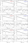Fig. 1.

Measured isotropic (top sub-panel in each panel) and anisotropic (bottom sub-panel in each panel, note the varying y-axis scale) shear signal around red (left) and blue (right) lenses in the NGVSLenS fields. From top to bottom: decreasing stellar mass bins as indicated. For better readability the anisotropic signal has been scaled by r. The best-fitting NFW shear profile constrained within 45 kpc/h₇₀ < r < 200 kpc/h₇₀ is shown by the curve for the isotropic signal. For (f − f₄₅)ΔΣ the curves show models computed from the best-fit isotropic model and the best-fit f_h for the solid curve, and f_h ∈ { + 1, 0, −1} for the dotted curves, respectively. The best-fit f_h has been constrained from (f − f₄₅)ΔΣ and ΔΣ within 45 kpc/h₇₀ < r < r_200c (range indicated by vertical lines), where r_200c has been estimated from the isotropic signal. The corresponding figures for the other surveys are shown in Appendix C.

In order to compute the average signal and error-bars shown in Fig. 1 we follow S15, first splitting the lens catalogues into patches covering ∼1 deg² (defined via the original survey pointings). For each patch we compute the profiles for each lens bin, employing larger cutouts from the mosaic source catalogue to ensure good coverage at the edges of a patch. For each lens colour and stellar mass bin we then compute the combined signal from all patches and thin lens redshift slices, weighting contributions according to their individual weight sums in the corresponding radial bin. Error-bars are then computed from 30 000 bootstrap re-samples of the contributing patches.

To robustly constrain halo shapes we aim to only include scales in the fit that are dominated by the host dark matter haloes of the lens galaxies. Following S15 we therefore include scales 45 kpc/h₇₀ < r < r_200c when constraining f_h, and scales 45 kpc/h₇₀ < r < 200 kpc/h₇₀ for an initial fit of the isotropic signal that is used to estimate r_200c and halo masses. Smaller scales can carry significant contributions from the baryonic matter distribution (see the small-scale increase in the isotropic signal in the top panels of Fig. 1), and for the lenses with the highest stellar mass these small scales also suffer from a dependence of the density of the selected sources on the position angle from the lens major axis (see S15). Larger radii are excluded from the fits as the shear profile may be significantly affected (see the excess isotropic signal at large radii in Fig. 1) either by neighbouring haloes or the parent halo if the lens is not a central galaxy but a satellite (see e.g., Velander et al. 2014, but we note that we apply cuts to reduce the fraction of satellites as explained in Sect. 3.2). Within our fit range the $\hat{Δ Σ} (r)$ $\widehat{\Delta\Sigma}(r)$ profiles are generally well described by the employed NFW models (see Figs. 1 and C.1–C.4).

Table 2 summarises the results we obtain for the different surveys and lens colour and stellar mass bins. Here we notice significant differences in the estimated halo masses between the different surveys for some of the colour and stellar mass bins. Uncertainties in the shape and redshift calibrations of the source galaxies may contribute to these differences, but we suspect that they are dominantly caused by differences in the stellar mass definitions of the different surveys (see Sect. 2). This is also hinted at by the fact that the lens ellipticity dispersion in particular lens colour and stellar mass bin combinations differs significantly between the different surveys (see Table 1). Likewise, the fractions of how many lenses fall into the different stellar mass bins vary between the surveys (compare Table 1). These differences in the stellar mass definitions, as well as the significant depth differences between the surveys are the main reasons why we initially analyse the surveys separately. However, this does not limit our ability to constrain f_h, given that the stellar masses are only used as a proxy to select approximately similar lenses within each particular lens bin.

Table 2.

Weak lensing constraints for the different stellar mass and colour bins in the different surveys, as well as joint f_h constraints.

Individual f_h constraints for the different surveys and lens bins are noisy (see Table 2), where the most significant (≃1.5 − 2σ) deviations from zero are found for the more massive red lenses in NGVSLenS and KV450. As explained in Sect. 3.4.3 we then compute joint constraints on f_h from the $\hat{Δ Σ} (r)$ $\widehat{\Delta \Sigma}(r)$ and $\hat{[f (r) - f_{45} (r)] Δ Σ_{iso} (r)}$ $\widehat{\left[f(r)-f_{45}(r)\right]\Delta \Sigma_{\mathrm{iso}}(r)}$ profiles of the different surveys. When including all surveys and stellar mass bins, we obtain $f_{h} = 0 . 303_{- 0.079}^{+ 0.080}$ $f_{\mathrm{h}}=0.303^{+0.080}_{-0.079}$ for red lenses, and $f_{h} = 0 . 217_{- 0.159}^{+ 0.160}$ $f_{\mathrm{h}}=0.217^{+0.160}_{-0.159}$ for blue lenses. These joint constraints are also indicated in Fig. 2, in which we plot the constraints on f_h versus M_200c for the individual surveys and stellar mass bins. Our results can also be compared to a recent halo shape analysis of the fourth KiDS data release (Georgiou et al. 2019b, see Fig. 2), which we discuss further in Sect. 5. Following S15 we alternatively drop the lowest stellar mass bin for red lenses, since this bin likely includes the highest fraction of satellite galaxies (e.g., Velander et al. 2014). In this case the resulting joint constraints $f_{h} = 0 . 304_{- 0.081}^{+ 0.083}$ $f_{\mathrm{h}}=0.304^{+0.083}_{-0.081}$ are essentially unchanged with only minimally inflated errors, suggesting that they are robust and dominated by the more massive lenses. We note that the χ²/d.o.f. values for the joint constraints are fully consistent with expected statistical fluctuations (see Table 2), corresponding to p-values of 0.31 (0.79) for the analysis combining all red (blue) lenses.

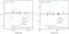Fig. 2.

Constraints on f_h and M_200c from the different surveys for red (left) and blue (right) lenses. For each survey, the different data points correspond to the different stellar mass bins. The horizontal solid and dotted lines mark the best-fit joint f_h constraints and the ±1σ limits, respectively. For comparison we also show results from the KiDS-1000 analysis of central galaxies from Georgiou et al. (2019b), including their default constraints and their results achieved using a wider weight function for the shape measurements (shown with an offset in mass for clarity).

For illustration we also show joint representations for the anisotropy of the shear field from all surveys and lens bins as a function of r/r_s in Fig. 3. To achieve this, we divide the measured (f − f₄₅)ΔΣ(r) profiles by the best-fit models for the spherical ΔΣ(r) profiles. As visible from the binned data points (shown in black) there is no significant radius-dependent deviation from the model prediction (f_rel − f_rel, 45)f_h, where f_h corresponds to the best-fit joint estimate for all red lenses and for all blue lenses, respectively.

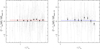Fig. 3.

Ratio of the measured (f − f₄₅)ΔΣ(r) profiles and the best-fit models for the spherical ΔΣ(r) profiles as a function of the radius in units of the NFW scale radius r_s. Left panel: red lenses, while blue lenses are shown on the right. Each grey point corresponds to one data point from Figs. 1 and C.1–C.4 (if it is located within the included fit range, see Sect. 4). Binned averages of these points are shown in black. The curves show model predictions (f_rel − f_rel, 45)f_h for the best-fit joint f_h estimates for all red lenses (left) and all blue lenses (right).

5. Discussion

Combining measurements from five different weak lensing surveys, we have been able to tighten constraints on halo ellipticity substantially compared to the previous CFHTLenS-only analysis conducted by S15, which employed the same methodology. While all surveys contribute to our new constraints, the most constraining contributions come from NGVSLenS and KV450 (compare Table 2), which is thanks to the excellent depth and superb seeing in the case of NGVS, and the excellent data quality and wide area in the case of KV450.

For red lenses we now obtain $f_{h} = 0 . 303_{- 0.079}^{+ 0.080}$ $f_{\mathrm{h}}=0.303^{+0.080}_{-0.079}$ (a 3.8σ detection of non-zero f_h), compared to $f_{h} = 0 . 217_{- 0.159}^{+ 0.160}$ $f_{\mathrm{h}}=0.217^{+0.160}_{-0.159}$ for blue lenses. These results are in excellent agreement with predictions that S15 derived using mock data based on the Millennium Simulation (Springel et al. 2005; Hilbert et al. 2009). The lens galaxy shapes for these mock data were initially computed by Joachimi et al. (2013b), employing the scheme from Heymans et al. (2006b). This assumes that the shapes of early-type galaxies follow those of their host dark matter haloes, while disc-dominated late-type galaxies are initially aligned such that their spin vector is parallel to the angular momentum vector of the corresponding host halo. Joachimi et al. (2013a) added misalignment between galaxies and their host dark matter haloes to these mock catalogues. For early-type galaxies they employed a Gaussian misalignment distribution with a scatter of 35°, as estimated from the distribution of satellites around SDSS luminous red galaxies (Okumura et al. 2009). This corresponds to a mean absolute misalignment angle of ∼28°, which is broadly consistent with results from hydrodynamical simulations (see Tenneti et al. 2014). For late-type galaxies Joachimi et al. (2013a) used the fitting function from Bett (2012), which was derived from simulated haloes that include baryons and incorporate models of galaxy formation physics (Bett et al. 2010; Deason et al. 2011; Crain et al. 2009; Okamoto et al. 2005). Combining lenses in halo mass ranges that are similar to our analysis, S15 estimate $f_{h} = 0 . 616_{- 0.005}^{+ 0.006}$ $f_{\mathrm{h}}=0.616_{-0.005}^{+0.006}$ (0.095 ± 0.005) for perfectly aligned early- (late-) type mock galaxies, which reduces to $f_{h} = 0 . 285_{- 0.004}^{+ 0.006}$ $f_{\mathrm{h}}=0.285_{-0.004}^{+0.006}$ ( $0 . 025_{- 0.004}^{+ 0.006}$ $0.025_{-0.004}^{+0.006}$ ) when including misalignment, in excellent agreement with our measurements. As a caveat we note that the early-type mock galaxies have noticeably lower intrinsic ellipticity dispersions compared to the real red lens galaxies. To account for this, S15 considered different schemes to re-scale their results which lower the f_h predictions from the simulation. If we rescale according to the factor ⟨|ϵ_g|⟩^surveys/⟨|ϵ_g|⟩^simulation = 1.53 (considering lenses with 0.05 < |ϵ_g| < 0.95) we would expect f_h ≃ 0.19 from the simulation, which is still consistent with our measurement for red lenses at the 1.5σ level.

The good agreement of our measurements with the current model predictions provides an important consistency check for galaxy formation models. This is also of direct relevance for cosmic shear measurements (e.g., Schrabback et al. 2010; Heymans et al. 2013; Jee et al. 2016; Troxel et al. 2018; Hamana et al. 2020; Asgari et al. 2020; Hildebrandt et al. 2020), which can be biased low due to shape–shear alignments (e.g., Hirata & Seljak 2004; Joachimi et al. 2015; Tugendhat & Schäfer 2018). These are caused by alignments of galaxies with their surrounding dark matter haloes and large-scale structure environments, which shear the images of background galaxies. This is linked to our measurements in two ways: First, the flattened halo contributes to the shearing of background galaxies and therefore the shape–shear alignments at small scales (Bridle & Abdalla 2007). Second, the misalignment between the lens shape and its surrounding dark matter distribution reduces the net strength of the shape–shear correlation. Constraints such as the ones derived from our analysis can therefore be used to update shape–shear corrections for cosmic shear. At large scales, these corrections can be calibrated from the alignment of galaxy ellipticities with their surrounding galaxy distributions, but at small scales (≲200 kpc) uncertainties regarding the galaxy bias prohibit the robust application of this approach (Hilbert et al. 2017). Fortunately, these are precisely the scales at which asymmetries in the matter distribution are probed by weak lensing analyses of galaxy halo shapes. We therefore suggest that future analyses of hydrodynamical simulations, which are used to constrain and calibrate intrinsic alignment models for cosmic shear (see e.g., Tenneti et al. 2016; Chisari et al. 2017; Hilbert et al. 2017; Piras et al. 2018), also provide direct predictions for f_h, which can then be compared to the observational constraints.

We stress the importance of comparing observational constraints on f_h to results from consistently analysed mock data, in order to properly account for imperfections in the analysis scheme. For example, the mock analysis from S15 shows that the systematics-corrected analysis scheme introduced by M06 is capable to approximately, but not perfectly, correct for the impact of cosmic shear and large-scale shape–shear correlations. Small residuals should however consistently occur in the real data and the mock analysis, thus allowing for a fair comparison. Likewise, our modelling approach assumes a linear scaling between galaxy ellipticity and halo ellipticity, as well as ellipticity-independent misalignment (see Sect. 3.4.2), neither of which assumptions is likely met exactly in reality. While this likely affects the absolute values of the resulting f_h constraints, this is not a concern for a relative comparison to predictions from simulations, as long as the same assumptions are made when analysing the simulated data. In particular, S15 make the same assumptions in their analysis of mock data, which is why our results are directly comparable to their predictions. Yet, in order to further improve future mock predictions, it will be important to further increase the realism of the galaxy shapes and misalignment models employed when creating the simulations.

Observational constraints on halo ellipticity have been obtained by a number of previous weak lensing studies. Among the earlier studies aiming to constrain halo ellipticity, Hoekstra et al. (2004) and Parker et al. (2007) analysed single-band imaging from RCS and CFHTLS without subdividing into red and blue lenses. Assuming elliptical truncated isothermal sphere models and conducting a maximum likelihood analysis, Hoekstra et al. (2004) obtained $f_{h} = 0 . 77_{- 0.21}^{+ 0.18}$ $f_{\mathrm{h}}=0.77^{+0.18}_{-0.21}$ , while Parker et al. (2007) investigated the ratio of the shears averaged in quadrants along the lens minor and major axes, yielding a tentative deviation from isotropy (they measured a mean ratio 0.76 ± 0.10 when including scales out to 70″). The f_h estimate from Hoekstra et al. (2004) is surprisingly high compared to our results. While the different assumptions regarding the density profiles affect f_h constraints (see M06), a more important reason for the discrepancy is likely given by the lack of a correction for the spurious signal caused by other sources of lens–source ellipticity alignments in the Hoekstra et al. (2004) analysis. Such alignments can bias f_h constraints low in the case of contributions from cosmic shear or consistently too large or too small PSF anisotropy corrections (M06). Likewise, they can bias them high for contributions from large-scale shape–shear correlations (S15). S15 argue that the latter effect may have biased the constraints from Hoekstra et al. (2004) high given that their data are relatively shallow, which leads to a stronger impact of shape–shear correlations compared to cosmic shear.

The methodology used in our analysis to correct for spurious signal was introduced by M06. Their analysis of SDSS data yielded f_h = 0.60 ± 0.38 for red and $f_{h} = - 1 . 4_{- 2.0}^{+ 1.7}$ $f_{\mathrm{h}}=-1.4^{+1.7}_{-2.0}$ for blue lenses when assuming elliptical NFW mass profiles. While these constraints are consistent with our results, they are likely affected by a sign error in the f₄₅ model prediction as identified by S15. The same is the case for the analysis of van Uitert et al. (2012), who find $f_{h} = 0 . 20_{- 1.31}^{+ 1.34}$ $f_{\mathrm{h}}=0.20^{+1.34}_{-1.31}$ for red lenses and $f_{h} = - 2 . 17_{- 2.03}^{+ 1.97}$ $f_{\mathrm{h}}=-2.17^{+1.97}_{-2.03}$ for blue lenses from RCS2 data when assuming elliptical NFW profiles and using the same lens ellipticity weighting as employed in our study. While we also incorporate RCS2 data into our study (RCSLenS), there are substantial differences. In particular, we employ lensfit shapes for the sources and fainter lenses (compared to KSB shapes for van Uitert et al. 2012), restrict the analysis to fields with four-band photometry (see Sect. 2.2), and only employ red lenses at 0.4 < z_b < 0.6 due to their better photo-z performance given the lack of u-band data (see Sect. 3.2). Most importantly, we apply the sign correction for the f₄₅ model (see Sect. 3.4.2). Together, this allows us to tighten the joint constraints for red lenses from RCS2 data noticeably compared to the previous results from van Uitert et al. (2012) to $f_{h} = 0 . 59_{- 0.66}^{+ 0.67}$ $f_{\mathrm{h}}=0.59_{-0.66}^{+0.67}$ (see Table 2 for results on the individual stellar mass bins). Nevertheless, RCSLenS provides the weakest contribution to our overall joint constraints from the five surveys (see Fig. 2). This is due to the comparably shallow source catalogue and the lack of u-band data, which leads to noisier photometric redshift estimates and causes us to only employ lenses in a narrower redshift range (see Sect. 3.2).

Within the uncertainties our measurements are fully consistent with the CFHTLenS results from S15, who used the same methodology as we do and obtained f_h = −0.04 ± 0.25 for red lenses and $f_{h} = 0 . 69_{- 0.36}^{+ 0.37}$ $f_{\mathrm{h}}=0.69_{-0.36}^{+0.37}$ for blue lenses. Their and our results are of course not independent given that we include CFHTLenS data in our analysis. Different to S15 we no longer remove z_b > 1.3 galaxies from our source sample, which leads to a moderate tightening of the CFHTLenS-only constraints in our analysis¹⁵ and shifts best-fitting values well within the error-bars to f_h = 0.09 ± 0.23 ( $f_{h} = 0 . 54_{- 0.32}^{+ 0.33}$ $f_{\mathrm{h}}=0.54^{+0.33}_{-0.32}$ ) for red (blue) lenses (see Table 2 for results on the individual stellar mass bins).

Very recently, the same methodology was applied by Georgiou et al. (2019b), who used data from the latest KiDS data release (Kuijken et al. 2019, KiDS-1000) to constrain f_h for a highly pure sample of central galaxies. In their default analysis they obtain f_h = 0.34 ± 0.17 for red lenses and f_h = 0.08 ± 0.53 for blue lenses, which increases to f_h = 0.55 ± 0.19 (f_h = 0.28 ± 0.55) for red (blue) lenses when they employ a 1.5 times wider weight function in the measurement of lens galaxy shapes using DEIMOS (Melchior et al. 2011). In our analysis we incorporate data from the previous KiDS KV-450 release, which covers slightly less than half of the area of KiDS-1000. A direct comparison between their and our study is complicated by differences in the lens selections, but we can attempt to match samples based on the estimated halo mass. Their blue sample is most similar to the blue KV-450 lenses in our highest stellar mass bin, for which we obtain f_h = 0.13 ± 0.55 in excellent agreement with both of their analyses schemes. Likewise, their red lenses are best matched by the combination of our two highest stellar mass bins of KV450 red lenses that yield f_h = 0.32 ± 0.14, which is in excellent agreement with their default analysis and still consistent with their results obtained using a wider weight function. Both studies achieve similar statistical uncertainties, where our photometric selection leads to a larger lens sample, which also extends to lower masses (compare Fig. 2). This is compensated by the larger sky area in their analysis. The increase Georgiou et al. (2019b) observe in their f_h constraints when using a wider weight function is interesting, as it also relates to recent results that suggest that central galaxies may be more aligned with their satellite distribution if their shapes are measured with more sensitivity to the galaxy outskirts (Huang et al. 2016; Georgiou et al. 2019a). We note that we also employ a slightly widened weight function when computing KSB+ moments for those galaxies without successful lensfit shape estimates (see Sect. 3.1). A detailed comparison to this aspect of the Georgiou et al. (2019b) results is complicated by differences between the shape measurement algorithms (lensfit and KSB+ versus DEIMOS), which is why we defer further investigations of the weight function-dependence of f_h constraints to future work.

A number of studies have also constrained halo ellipticity at the mass scale of galaxy groups and clusters. For example, van Uitert et al. (2017) constrain the average halo ellipticity of groups in the GAMA survey using KiDS weak lensing data assuming elliptical NFW density profiles. They find that the shear signal around the brightest group/cluster member (BCG) shows substantial anisotropy at scales r < 250 kpc, which yields an average halo ellipticity of ⟨|ϵ_h|⟩ = 0.38 ± 0.12 when assuming perfect alignment with the BCG orientation. At larger scales their signal becomes isotropic with respect to the BCG orientation, but still remains anisotropic when compared to the spatial distribution of group members. Clampitt & Jain (2016) constrain the anisotropy in the lensing signal around luminous red galaxies (LRGs) that are similar to the BCGs from van Uitert et al. (2017) yielding a smaller value ⟨|ϵ_h|⟩ = 0.12 ± 0.03 (in our ellipticity definition). Building up on this work, Shin et al. (2018) infer a best-fit average axis ratio of q = 0.56 ± 0.09(stat.)±0.03(sys.) in the mass distribution for a weak lensing analysis of redMaPPer (Rykoff et al. 2014) clusters, corresponding to ⟨|ϵ_h|⟩ = 0.28 ± 0.08. At higher masses, using weak lensing data of strong lensing clusters and employing the strong lensing constraints as a proxy for the orientation of the halo, Oguri et al. (2012) obtain ⟨|ϵ_h|⟩ = 0.31 ± 0.05. Similarly, Umetsu et al. (2018) combine weak lensing shear and magnification measurements of 20 massive CLASH clusters to obtain ⟨|ϵ_h|⟩ = 0.20 ± 0.05 (when using our ellipticity definition).

It is important to realise that these constraints are obtained at significantly higher mass scales (see Fig. 4 for an approximate comparison). For example, the group sample from van Uitert et al. (2017) yields an average mass $M_{200 c} = 1 . 50_{- 0.24}^{+ 0.25} \times 10^{13} M_{⊙}$ $M_{\mathrm{200c}}=1.50^{+0.25}_{-0.24}\times 10^{13}\,{M_\odot}$ , which is still higher by factors of ∼2, ∼7, and ∼16, respectively, compared to what we typically find for our red lens samples in the three stellar mass bins (compare Table 2). Considering all red lenses in the five surveys that fall into these stellar mass bins and pass the selections (but without applying the |ϵ_g|> 0.05 cut), the average absolute value of the lens ellipticity amounts to ⟨|ϵ_g|⟩ = 0.265. If galaxies and haloes were perfectly aligned, our estimate of $f_{h} = 0 . 303_{- 0.079}^{+ 0.080}$ $f_{\mathrm{h}}=0.303^{+0.080}_{-0.079}$ for these lenses would then imply ⟨|ϵ_h|⟩ = 0.08 ± 0.02. We can correct this estimate for the impact of misalignment by considering results from S15: In their analysis of mock data based on the Millennium Simulation, S15 investigate both cases of perfectly aligned and misaligned galaxy-halo pairs. Assuming their employed misalignment models (as implemented by Joachimi et al. 2013a) are correct we can use the ratio of their resulting f_h estimates for these cases¹⁶f_h(aligned)/f_h(misaligned) = 2.16 to correct our halo ellipticity estimate for red lenses, yielding ⟨|ϵ_h|⟩ = 0.174 ± 0.046. This is still lower compared to the above-mentioned results for group and cluster-scale haloes, consistent with expectations from numerical simulations, which suggest that less massive haloes are more spherical (e.g., Bailin & Steinmetz 2005; Despali et al. 2014; Vega-Ferrero et al. 2017; Despali et al. 2017). The only exception is the constraint for the LRG sample from Clampitt & Jain (2016), which is lower, but still consistent with our misalignment-corrected estimate. However, given that their results do not include a misalignment correction, the true halo ellipticity is likely larger for their sample.

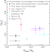Fig. 4.

Comparison of constraints on ⟨|ϵ_h|⟩ for red galaxies, galaxy groups, and galaxy clusters from different studies. For our study we combine the constraints from all red lens samples for our two highest stellar mass bins, showing both the uncorrected estimate (assuming perfect alignment of galaxies and haloes), and the more realistic misalignment-corrected estimate. The latter assumes that the impact of misalignment is correctly described by the comparison of the results from the S15 Millennium Simulation analyses with and without misalignment (see Sect. 5). The horizontal error-bars indicate the approximate lens mass range for our results as well as the studies from Oguri et al. (2012), Shin et al. (2018) and Umetsu et al. (2018). For van Uitert et al. (2017) the data point is shown at their best-fit mean mass, where the error corresponds to the fit uncertainty. Clampitt & Jain (2016) only report an approximate mean mass for their sample. We apply mass conversions in case authors employ other definitions than M_200c.

6. Conclusions

We have combined weak lensing data from five surveys (CFHTLenS, NGVSLenS, CS82, RCSLenS, and KiDS/KV450) in order to tightly constrain f_h = ⟨cos(2Δϕ_h, g)|ϵ_h|/|ϵ_g|⟩ the average aligned component of the ellipticity ratio between the host dark matter halo and its embedded galaxy for photometrically selected lens galaxies at redshifts 0.2 < z_b < 0.6. We obtain $f_{h} = 0 . 303_{- 0.079}^{+ 0.080}$ $f_{\mathrm{h}}=0.303^{+0.080}_{-0.079}$ for red lenses. Similarly clear signals of dark matter halo flattening have previously been reported at the mass scale of galaxy groups and clusters (e.g., Oguri et al. 2012; Clampitt & Jain 2016; van Uitert et al. 2017), but to our knowledge this presently constitutes the most significant (3.8σ) systematics-corrected detection at the mass scale of galaxies. We measure $f_{h} = 0 . 217_{- 0.159}^{+ 0.160}$ $f_{\mathrm{h}}=0.217^{+0.160}_{-0.159}$ for blue galaxies, consistent with a non-detection. Both results are in good agreement with theoretical predictions obtained by S15 using mock data from the Millennium Simulation when including models for galaxy-halo misalignment. If we assume that the misalignment models employed in the mock data for early-type galaxies are correct (Gaussian misalignment distribution with a scatter of 35°, see Okumura et al. 2009; Joachimi et al. 2013a), we can infer an average halo ellipticity of ⟨|ϵ_h|⟩ = 0.174 ± 0.046 for our red lens galaxies. This is lower compared to most measurements derived at the scale of galaxy groups and galaxy clusters (Evans & Bridle 2009; Oguri et al. 2012; Clampitt & Jain 2016; van Uitert et al. 2017; Shin et al. 2018; Umetsu et al. 2018), as consistent with the expectation from simulations that less massive haloes are more spherical (e.g., Bailin & Steinmetz 2005; Despali et al. 2014; Vega-Ferrero et al. 2017).

Observational constraints on f_h sensitively test theoretical models that describe the co-evolution of galaxies and their host dark matter haloes. Improving and better calibrating these models is essential in order to reduce systematic uncertainties in cosmological weak lensing surveys related to intrinsic galaxy alignments (see e.g., Tenneti et al. 2016; Chisari et al. 2017; Hilbert et al. 2017; Piras et al. 2018). Beyond this, constraints on halo ellipticity can also be used to test non-standard cosmological models. For example, interacting dark matter models predict more spherical dark matter haloes (Hellwing et al. 2013; Peter et al. 2013). This is also the case for coupled dark energy models, while the opposite seems to be the case for f(R) theories (L’Huillier et al. 2017). The predicted differences of these models compared to standard ΛCDM expectations are however small, requiring the constraining power of future weak lensing surveys to potentially become useful tests. This may be different for theories of modified gravity that aim to remove the need for dark matter, including MOND (Modified Newtonian Dynamics, Milgrom 1983), TeVeS (Scalar–Tensor–Vector theory, Bekenstein 2004), and MOG/STVG (Modified Gravity and Scalar–Tensor–Vector Gravity theory, Moffat 2006; Moffat & Toth 2009). When considering isolated galaxies in such cosmologies one would naively expect nearly isotropic gravitational signatures at large separations from the baryons (e.g., Milgrom 2001). This seems to be at odds with our 3.8σ detection of non-zero f_h for red galaxies. Unfortunately, detailed forecasts for expected f_h estimates in such cosmologies are not yet available. If such predictions are developed in the future, they would likely need to incorporate the potentially contaminating impact of the surrounding large-scale structure, as included in the ΛCDM mock estimates from S15, which we compare our measurements to.

Observationally the future is bright for halo ellipticity measurements. Next generation weak lensing surveys such as Euclid (Laureijs et al. 2011) and LSST (LSST Science Collaboration 2009) will provide a tremendous statistical constraining power, providing the prospects to tightly constrain halo ellipticity signatures for different galaxy samples both as a function of mass scale and redshift (simulations predict more spherical haloes at lower redshifts and lower masses, see e.g., Tenneti et al. 2014). The sensitivity of these surveys may also yield significant detections using estimators that include the ellipticities of lenses and pairs of background sources, providing a route to separate the currently degenerate signatures of halo sphericity and misalignment (e.g., Schneider & Watts 2005; Simon et al. 2012; Adhikari et al. 2015; Shirasaki & Yoshida 2018).

¹

In weak lensing estimates of f_h, weights that depend on |ϵ_g| are typically applied in the averaging, see Sect. 3.4.2.

²

f_h is computed from the ratio of the isotropic and the anisotropic lensing signals (see Sect. 3.4), which is why the cosmology dependence cancels out to leading order. Within the fit range the model expectation is only marginally radius dependent (see Fig. 3), which is why the cosmology dependence of the radius can be well neglected.

³

CFHTLenS: http://www.cadc-ccda.hia-iha.nrc-cnrc.gc.ca/en/community/CFHTLens

⁴

RCSLenS: https://www.cadc-ccda.hia-iha.nrc-cnrc.gc.ca/en/community/rcslens

⁵

KV450: http://kids.strw.leidenuniv.nl/cosmicshear2018.php

⁶

We also verified that shape measurements agree well between KSB+ and lensfit for bright galaxies that are not removed by lensfit.

⁷

We employ a weight function with a scale radius that is larger by a factor of $\sqrt{2}$ $\sqrt{2}$ compared to the Gaussian scale radius that would optimise the signal-to-noise ratio in the case of Gaussian brightness profiles.

⁸

To remove stars we employ the SExtractor CLASS_STAR parameter, requiring CLASS_STAR < 0.5. To be consistent with S15 we additionally require star_flag = 0 for CFHTLenS and apply a similar selection SG_FLAG = 1 for RCSLenS as recommended by these surveys. We however find that these latter cuts have a completely negligible impact, removing < 0.2% of the otherwise selected lens candidates only. We verified through visual inspection that our final lens samples do not suffer from a significant contamination by stars.

⁹

This is the case for ≳98% of the lens candidates.

¹⁰

Bundy et al. (2015) provide a stellar mass catalogue, but we do not employ it in our analysis since it only covers a part of the footprint of our CS82 analysis.

¹¹

On average this cut removes about 16% of the lens candidates in this colour and stellar mass bin.

¹²

Structures in front of the lens do not contribute to the net isotropic galaxy-galaxy lensing signal, but can cause spurious signal for weak lensing constraints on halo ellipticity for simple estimators (this is corrected for in our analysis, see Sect. 3.4.2). Structures behind the lens do not cause any bias.

¹³

We note, however, that the isotropic shear profile and therefore $\hat{x} (r)$ $\widehat{x}(r)$ is typically well constrained (see Figs. 1 and C.1–C.4), which is why the uncertainties in $\hat{y} (r)$ $\widehat{\mathit{y}}(r)$ have the biggest impact on the uncertainties of the f_h estimates.

¹⁴

We note that there is a typo in the corresponding equation in S15, but their results were computed correctly.

¹⁵

This is thanks to the high lensing efficiency weights of the z_b > 1.3 sources and their non-negligible number (e.g., they constitute 29% of all CFHTLenS sources with z_b > 0.7).

¹⁶

Using their combination of early-type lenses at 0.2 ≤ z_l < 0.6 with 9.5 < log₁₀M_* < 11 to best match our halo mass range.

¹⁷

In Sect. 3.4 we denoted these estimates as $\hat{[f (r) - f_{45} (r)] Δ Σ_{iso} (r)}$ $\widehat{\left[f(r)-f_{45}(r)\right]\Delta \Sigma_{\mathrm{iso}}(r)}$ to stress that the model expectations for f and f₄₅ are radius dependent. However, within our fit range the radius dependence is weak for f(r)−f₄₅(r), as indicated by the almost flat curves in Fig. 3. Thus, and to improve the readability we employ this shortened notation here and in the y-axis labels of Figs. 1, 3, and C.1–C.4.

¹⁸

Confirming results from S15 we find that the off-diagonal entries in the correlation matrix are generally small. For example, for the KV-450 data within our fit range the off-diagonal entries in the correlation matrix (including the cross-correlation between $\hat{Δ Σ_{iso}} (r)$ $\widehat{\Delta \Sigma_{\mathrm{iso}}}(r)$ and $\hat{[f - f_{45}] Δ Σ_{iso} (r)}$ $\widehat{\left[f-f_{45} \right]\Delta \Sigma_{\mathrm{iso}}(r)}$ ) have an rms of 0.05 (likely limited by noise from the covariance estimation via the field-wise bootstrapping) and have absolute values that are always < 0.15.

Acknowledgments

We thank Rachel Mandelbaum for providing the tabulated model predictions for the anisotropic shear signal. We also thank the anonymous referee, whose comments have helped to improve the paper significantly. This work is based on observations obtained with MegaPrime/MegaCam, a joint project of CFHT and CEA/DAPNIA, at the Canada-France-Hawaii Telescope (CFHT) which is operated by the National Research Council (NRC) of Canada, the Institut National des Sciences de l’Univers of the Centre National de la Recherche Scientifique (CNRS) of France, and the University of Hawaii. This research used the facilities of the Canadian Astronomy Data Centre operated by the National Research Council of Canada with the support of the Canadian Space Agency. RCSLenS data processing was made possible thanks to significant computing support from the NSERC Research Tools and Instruments grant program. CS82 is a joint project using Canadian, French and Brazilian time on CFHT (programmes 10BB009, 10BF023 and 10BC022). The Brazilian partnership on CFHT was managed by the Laboratório Nacional de Astrofísica (LNA). Based on data products from observations made with ESO Telescopes at the La Silla Paranal Observatory under programme IDs 177.A-3016, 177.A-3017, 177.A-3018, 179.A-2004, 298.A-5015, and on data products produced by the KiDS consortium. HH and AK acknowledge support from Vici grant 639.043.512 financed by the Netherlands Organization for Scientic Research. EvU acknowledges support from an STFC Ernest Rutherford Research Grant, grant reference ST/L00285X/1. LvW is funded by NSERC and CIfAR. CH and MA acknowledge support from the European Research Council under grant number 647112. CH also acknowledges support from the Max Planck Society and the Alexander von Humboldt Foundation in the framework of the Max Planck-Humboldt Research Award endowed by the Federal Ministry of Education and Research. HHi is supported by a Heisenberg grant of the Deutsche Forschungsgemeinschaft (Hi 1495/5-1) as well as an ERC Consolidator Grant (No. 770935). LM acknowledges support from STFC grant ST/N000919/1. Author Contributions. All authors contributed to the development and writing of this paper. The authorship list is given in two groups: the lead authors (TS, HH, LVW, EvU, CG), followed by an alphabetical group, which covers those who have either made a significant contribution to the data products or to the scientific analysis.

References

Adelman-McCarthy, J. K., Agüeros, M. A., Allam, S. S., et al. 2007, ApJS, 172, 634 [NASA ADS] [CrossRef] [Google Scholar]
Adhikari, S., Chue, C. Y. R., & Dalal, N. 2015, JCAP, 1, 9 [Google Scholar]
Agustsson, I., & Brainerd, T. G. 2010, ApJ, 709, 1321 [NASA ADS] [CrossRef] [Google Scholar]
Annis, J., Soares-Santos, M., Strauss, M. A., et al. 2014, ApJ, 794, 120 [NASA ADS] [CrossRef] [Google Scholar]
Arnouts, S., Cristiani, S., Moscardini, L., et al. 1999, MNRAS, 310, 540 [NASA ADS] [CrossRef] [Google Scholar]
Asgari, M., Tröster, T., Heymans, C., et al. 2020, A&A, 634, A127 [NASA ADS] [CrossRef] [EDP Sciences] [Google Scholar]
Bailin, J., & Steinmetz, M. 2005, ApJ, 627, 647 [Google Scholar]
Bartelmann, M., & Schneider, P. 2001, Phys. Rep., 340, 291 [NASA ADS] [CrossRef] [Google Scholar]
Bate, J., Chisari, N. E., Codis, S., et al. 2020, MNRAS, 491, 4057 [Google Scholar]
Begeman, K., Belikov, A. N., Boxhoorn, D. R., & Valentijn, E. A. 2013, Exp. Astron., 35, 1 [NASA ADS] [Google Scholar]
Bekenstein, J. D. 2004, Phys. Rev. D, 70, 083509 [Google Scholar]
Benítez, N. 2000, ApJ, 536, 571 [Google Scholar]
Bertin, E., & Arnouts, S. 1996, A&AS, 117, 393 [NASA ADS] [CrossRef] [EDP Sciences] [Google Scholar]
Bett, P. 2012, MNRAS, 420, 3303 [NASA ADS] [CrossRef] [Google Scholar]
Bett, P., Eke, V., Frenk, C. S., Jenkins, A., & Okamoto, T. 2010, MNRAS, 404, 1137 [NASA ADS] [Google Scholar]
Bhowmick, A. K., Chen, Y., Tenneti, A., Di Matteo, T., & Mandelbaum, R. 2020, MNRAS, 491, 4116 [Google Scholar]
Bliss, C. I. 1935a, Ann. Appl. Biol., 22, 134 [CrossRef] [Google Scholar]
Bliss, C. I. 1935b, Ann. Appl. Biol., 22, 307 [Google Scholar]
Brainerd, T. G., & Wright, C. O. 2000, ArXiv e-prints [arXiv:astro-ph/0006281] [Google Scholar]
Brammer, G. B., van Dokkum, P. G., & Coppi, P. 2008, ApJ, 686, 1503 [NASA ADS] [CrossRef] [Google Scholar]
Bridle, S., & Abdalla, F. B. 2007, ApJ, 655, L1 [NASA ADS] [CrossRef] [Google Scholar]
Bridle, S., & King, L. 2007, New J. Phys., 9, 444 [NASA ADS] [CrossRef] [Google Scholar]
Bruderer, C., Read, J. I., Coles, J. P., et al. 2016, MNRAS, 456, 870 [Google Scholar]
Bundy, K., Leauthaud, A., Saito, S., et al. 2015, ApJS, 221, 15 [NASA ADS] [CrossRef] [Google Scholar]
Bundy, K., Leauthaud, A., Saito, S., et al. 2017, ApJ, 851, 34 [Google Scholar]
Caminha, G. B., Grillo, C., Rosati, P., et al. 2016, A&A, 587, A80 [NASA ADS] [CrossRef] [EDP Sciences] [Google Scholar]
Caminha, G. B., Rosati, P., Grillo, C., et al. 2019, A&A, 632, A36 [CrossRef] [EDP Sciences] [Google Scholar]
Chisari, N. E., Koukoufilippas, N., Jindal, A., et al. 2017, MNRAS, 472, 1163 [Google Scholar]
Choi, A., Heymans, C., Blake, C., et al. 2016, MNRAS, 463, 3737 [NASA ADS] [CrossRef] [Google Scholar]
Chua, K. T. E., Pillepich, A., Vogelsberger, M., & Hernquist, L. 2019, MNRAS, 484, 476 [CrossRef] [Google Scholar]
Clampitt, J., & Jain, B. 2016, MNRAS, 457, 4135 [NASA ADS] [CrossRef] [Google Scholar]
Codis, S., Jindal, A., Chisari, N. E., et al. 2018, MNRAS, 481, 4753 [CrossRef] [Google Scholar]
Coe, D., Benítez, N., Sánchez, S. F., et al. 2006, AJ, 132, 926 [NASA ADS] [CrossRef] [Google Scholar]
Crain, R. A., Theuns, T., Dalla Vecchia, C., et al. 2009, MNRAS, 399, 1773 [NASA ADS] [CrossRef] [Google Scholar]
de Jong, J. T. A., Verdoes Kleijn, G. A., Erben, T., et al. 2017, A&A, 604, A134 [NASA ADS] [CrossRef] [EDP Sciences] [Google Scholar]
Deason, A. J., McCarthy, I. G., Font, A. S., et al. 2011, MNRAS, 415, 2607 [NASA ADS] [CrossRef] [Google Scholar]
Debattista, V. P., van den Bosch, F. C., Roškar, R., et al. 2015, MNRAS, 452, 4094 [Google Scholar]
Despali, G., Giocoli, C., & Tormen, G. 2014, MNRAS, 443, 3208 [NASA ADS] [CrossRef] [Google Scholar]
Despali, G., Giocoli, C., Bonamigo, M., Limousin, M., & Tormen, G. 2017, MNRAS, 466, 181 [NASA ADS] [CrossRef] [Google Scholar]
Diego, J. M., Broadhurst, T., Benitez, N., Lim, J., & Lam, D. 2015, MNRAS, 449, 588 [Google Scholar]
Duffy, A. R., Schaye, J., Kay, S. T., & Dalla Vecchia, C. 2008, MNRAS, 390, L64 [NASA ADS] [CrossRef] [Google Scholar]
Dvornik, A., Zoutendijk, S. L., Hoekstra, H., & Kuijken, K. 2019, A&A, 627, A74 [CrossRef] [EDP Sciences] [Google Scholar]
Erben, T., Hildebrandt, H., Lerchster, M., et al. 2009, A&A, 493, 1197 [NASA ADS] [CrossRef] [EDP Sciences] [Google Scholar]
Erben, T., Hildebrandt, H., Miller, L., et al. 2013, MNRAS, 433, 2545 [Google Scholar]
Evans, A. K. D., & Bridle, S. 2009, ApJ, 695, 1446 [NASA ADS] [CrossRef] [EDP Sciences] [Google Scholar]
Fenech Conti, I., Herbonnet, R., Hoekstra, H., et al. 2017, MNRAS, 467, 1627 [NASA ADS] [Google Scholar]
Ferrarese, L., Côté, P., Cuillandre, J. C., et al. 2012, ApJS, 200, 4 [NASA ADS] [CrossRef] [Google Scholar]
Fieller, E. C. 1954, J. R. Stat. Soc. B, 16, 175 [Google Scholar]
Georgiou, C., Chisari, N. E., Fortuna, M. C., et al. 2019a, A&A, 628, A31 [EDP Sciences] [Google Scholar]
Georgiou, C., Hoekstra, H., Kuijken, K., et al. 2019b, A&A, submitted [Google Scholar]
Gilbank, D. G., Gladders, M. D., Yee, H. K. C., & Hsieh, B. C. 2011, AJ, 141, 94 [NASA ADS] [CrossRef] [Google Scholar]
Hamana, T., Shirasaki, M., Miyazaki, S., et al. 2020, PASJ, 72, 16 [CrossRef] [Google Scholar]
Hand, N., Leauthaud, A., Das, S., et al. 2015, Phys. Rev. D, 91, 062001 [CrossRef] [Google Scholar]
Harvey, D., Tam, S. I., Jauzac, M., Massey, R., & Rhodes, J. 2019, MNRAS, submitted [arXiv:1911.06333] [Google Scholar]
Hayashi, K., & Chiba, M. 2014, ApJ, 789, 62 [Google Scholar]
Hellwing, W. A., Cautun, M., Knebe, A., Juszkiewicz, R., & Knollmann, S. 2013, JCAP, 2013, 012 [CrossRef] [Google Scholar]
Heymans, C., Van Waerbeke, L., Bacon, D., et al. 2006a, MNRAS, 368, 1323 [NASA ADS] [CrossRef] [Google Scholar]
Heymans, C., White, M., Heavens, A., Vale, C., & van Waerbeke, L. 2006b, MNRAS, 371, 750 [NASA ADS] [CrossRef] [Google Scholar]
Heymans, C., Van Waerbeke, L., Miller, L., et al. 2012, MNRAS, 427, 146 [NASA ADS] [CrossRef] [Google Scholar]
Heymans, C., Grocutt, E., Heavens, A., et al. 2013, MNRAS, 432, 2433 [NASA ADS] [CrossRef] [Google Scholar]
Hilbert, S., Hartlap, J., White, S. D. M., & Schneider, P. 2009, A&A, 499, 31 [NASA ADS] [CrossRef] [EDP Sciences] [Google Scholar]
Hilbert, S., Xu, D., Schneider, P., et al. 2017, MNRAS, 468, 790 [Google Scholar]
Hildebrandt, H., Erben, T., Kuijken, K., et al. 2012, MNRAS, 421, 2355 [Google Scholar]
Hildebrandt, H., Choi, A., Heymans, C., et al. 2016, MNRAS, 463, 635 [NASA ADS] [CrossRef] [Google Scholar]
Hildebrandt, H., Viola, M., Heymans, C., et al. 2017, MNRAS, 465, 1454 [Google Scholar]
Hildebrandt, H., Köhlinger, F., van den Busch, J. L., et al. 2020, A&A, 633, A69 [NASA ADS] [CrossRef] [EDP Sciences] [Google Scholar]
Hirata, C. M., & Seljak, U. 2004, Phys. Rev. D, 70, 063526 [NASA ADS] [CrossRef] [Google Scholar]
Hoekstra, H., Franx, M., Kuijken, K., & Squires, G. 1998, ApJ, 504, 636 [NASA ADS] [CrossRef] [Google Scholar]
Hoekstra, H., Franx, M., & Kuijken, K. 2000, ApJ, 532, 88 [NASA ADS] [CrossRef] [Google Scholar]
Hoekstra, H., Yee, H. K. C., & Gladders, M. D. 2004, ApJ, 606, 67 [NASA ADS] [CrossRef] [Google Scholar]
Huang, H.-J., Mandelbaum, R., Freeman, P. E., et al. 2016, MNRAS, 463, 222 [NASA ADS] [CrossRef] [Google Scholar]
Ilbert, O., Arnouts, S., McCracken, H. J., et al. 2006, A&A, 457, 841 [NASA ADS] [CrossRef] [EDP Sciences] [Google Scholar]
Jauzac, M., Harvey, D., & Massey, R. 2018, MNRAS, 477, 4046 [NASA ADS] [CrossRef] [Google Scholar]
Jee, M. J., Tyson, J. A., Hilbert, S., et al. 2016, ApJ, 824, 77 [NASA ADS] [CrossRef] [Google Scholar]
Jing, Y. P., & Suto, Y. 2002, ApJ, 574, 538 [NASA ADS] [CrossRef] [Google Scholar]
Joachimi, B., Semboloni, E., Hilbert, S., et al. 2013a, MNRAS, 436, 819 [Google Scholar]
Joachimi, B., Semboloni, E., Bett, P. E., et al. 2013b, MNRAS, 431, 477 [NASA ADS] [CrossRef] [Google Scholar]
Joachimi, B., Cacciato, M., Kitching, T. D., et al. 2015, Space Sci. Rev., 193, 1 [NASA ADS] [CrossRef] [Google Scholar]
Kacprzak, T., Zuntz, J., Rowe, B., et al. 2012, MNRAS, 427, 2711 [NASA ADS] [CrossRef] [Google Scholar]
Kaiser, N. 1995, ApJ, 439, L1 [NASA ADS] [CrossRef] [Google Scholar]
Kaiser, N., Squires, G., & Broadhurst, T. 1995, ApJ, 449, 460 [NASA ADS] [CrossRef] [Google Scholar]
Kannawadi, A., Hoekstra, H., Miller, L., et al. 2019, A&A, 624, A92 [NASA ADS] [CrossRef] [EDP Sciences] [Google Scholar]
Khoperskov, S. A., Moiseev, A. V., Khoperskov, A. V., & Saburova, A. S. 2014, MNRAS, 441, 2650 [NASA ADS] [CrossRef] [Google Scholar]
Kitching, T. D., Miller, L., Heymans, C. E., van Waerbeke, L., & Heavens, A. F. 2008, MNRAS, 390, 149 [NASA ADS] [CrossRef] [Google Scholar]
Kuijken, K., Heymans, C., Hildebrandt, H., et al. 2015, MNRAS, 454, 3500 [Google Scholar]
Kuijken, K., Heymans, C., Dvornik, A., et al. 2019, A&A, 625, A2 [NASA ADS] [CrossRef] [EDP Sciences] [Google Scholar]
Laigle, C., Pichon, C., Codis, S., et al. 2015, MNRAS, 446, 2744 [NASA ADS] [CrossRef] [Google Scholar]
Laureijs, R., Amiaux, J., Arduini, S., et al. 2011, ArXiv e-prints [arXiv:1110.3193] [Google Scholar]
Leauthaud, A., Saito, S., Hilbert, S., et al. 2017, MNRAS, 467, 3024 [NASA ADS] [CrossRef] [Google Scholar]
L’Huillier, B., Winther, H. A., Mota, D. F., Park, C., & Kim, J. 2017, MNRAS, 468, 3174 [NASA ADS] [CrossRef] [Google Scholar]
Limousin, M., Morandi, A., Sereno, M., et al. 2013, Space Sci. Rev., 177, 155 [NASA ADS] [CrossRef] [Google Scholar]
Liu, X., Pan, C., Li, R., et al. 2015, MNRAS, 450, 2888 [NASA ADS] [CrossRef] [Google Scholar]
LSST Science Collaboration (Abell, P. A., et al.) 2009, ArXiv e-prints [arXiv:0912.0201] [Google Scholar]
Luppino, G. A., & Kaiser, N. 1997, ApJ, 475, 20 [NASA ADS] [CrossRef] [Google Scholar]
Mandelbaum, R., Hirata, C. M., Broderick, T., Seljak, U., & Brinkmann, J. 2006, MNRAS, 370, 1008 [NASA ADS] [CrossRef] [Google Scholar]
Massey, R., Heymans, C., Bergé, J., et al. 2007, MNRAS, 376, 13 [Google Scholar]
Melchior, P., & Viola, M. 2012, MNRAS, 424, 2757 [Google Scholar]
Melchior, P., Viola, M., Schäfer, B. M., & Bartelmann, M. 2011, MNRAS, 412, 1552 [NASA ADS] [CrossRef] [Google Scholar]
Milgrom, M. 1983, ApJ, 270, 365 [NASA ADS] [CrossRef] [Google Scholar]
Milgrom, M. 2001, MNRAS, 326, 1261 [Google Scholar]
Miller, L., Kitching, T. D., Heymans, C., Heavens, A. F., & van Waerbeke, L. 2007, MNRAS, 382, 315 [Google Scholar]
Miller, L., Heymans, C., Kitching, T. D., et al. 2013, MNRAS, 429, 2858 [Google Scholar]
Miralda-Escude, J. 1991, ApJ, 370, 1 [NASA ADS] [CrossRef] [Google Scholar]
Moffat, J. W. 2006, JCAP, 3, 4 [NASA ADS] [CrossRef] [Google Scholar]
Moffat, J. W., & Toth, V. T. 2009, MNRAS, 397, 1885 [NASA ADS] [CrossRef] [Google Scholar]
Natarajan, P., & Refregier, A. 2000, ApJ, 538, L113 [NASA ADS] [CrossRef] [Google Scholar]
Navarro, J. F., Frenk, C. S., & White, S. D. M. 1996, ApJ, 462, 563 [Google Scholar]
Navarro, J. F., Frenk, C. S., & White, S. D. M. 1997, ApJ, 490, 493 [NASA ADS] [CrossRef] [Google Scholar]
Oguri, M., Takada, M., Okabe, N., & Smith, G. P. 2010, MNRAS, 405, 2215 [NASA ADS] [Google Scholar]
Oguri, M., Bayliss, M. B., Dahle, H., et al. 2012, MNRAS, 420, 3213 [NASA ADS] [CrossRef] [Google Scholar]
Okamoto, T., Eke, V. R., Frenk, C. S., & Jenkins, A. 2005, MNRAS, 363, 1299 [NASA ADS] [CrossRef] [Google Scholar]
Okumura, T., Jing, Y. P., & Li, C. 2009, ApJ, 694, 214 [NASA ADS] [CrossRef] [Google Scholar]
Parker, L. C., Hoekstra, H., Hudson, M. J., van Waerbeke, L., & Mellier, Y. 2007, ApJ, 669, 21 [NASA ADS] [CrossRef] [Google Scholar]
Parroni, C., Mei, S., Erben, T., et al. 2017, ApJ, 848, 114 [NASA ADS] [CrossRef] [Google Scholar]
Paterno-Mahler, R., Sharon, K., Coe, D., et al. 2018, ApJ, 863, 154 [Google Scholar]
Peter, A. H. G., Rocha, M., Bullock, J. S., & Kaplinghat, M. 2013, MNRAS, 430, 105 [Google Scholar]
Peters, S. P. C., van der Kruit, P. C., Allen, R. J., & Freeman, K. C. 2017, MNRAS, 464, 65 [Google Scholar]
Piras, D., Joachimi, B., Schäfer, B. M., et al. 2018, MNRAS, 474, 1165 [NASA ADS] [CrossRef] [Google Scholar]
Planck Collaboration VI. 2020, A&A, 641, A6 [NASA ADS] [CrossRef] [EDP Sciences] [Google Scholar]
Raichoor, A., Mei, S., Erben, T., et al. 2014, ApJ, 797, 102 [NASA ADS] [CrossRef] [Google Scholar]
Refregier, A., Kacprzak, T., Amara, A., Bridle, S., & Rowe, B. 2012, MNRAS, 425, 1951 [Google Scholar]
Rykoff, E. S., Rozo, E., Busha, M. T., et al. 2014, ApJ, 785, 104 [NASA ADS] [CrossRef] [Google Scholar]
Schäfer, B. M., & Merkel, P. M. 2017, MNRAS, 470, 3453 [Google Scholar]
Schneider, P., & Watts, P. 2005, A&A, 432, 783 [NASA ADS] [CrossRef] [EDP Sciences] [Google Scholar]
Schneider, P., Kochanek, C., & Wambsganss, J. 2006, in Gravitational Lensing: Strong, Weak & Micro, Saas-Fee Advanced Course 33, eds. G. Meylan, P. Jetzer, & P. North (Berlin: Springer-Verlag), Swiss Soc. Astrophys. Astron. [Google Scholar]
Schrabback, T., Hartlap, J., Joachimi, B., et al. 2010, A&A, 516, A63 [NASA ADS] [CrossRef] [EDP Sciences] [Google Scholar]
Schrabback, T., Hilbert, S., Hoekstra, H., et al. 2015, MNRAS, 454, 1432 [Google Scholar]
Schrabback, T., Applegate, D., Dietrich, J. P., et al. 2018, MNRAS, 474, 2635 [Google Scholar]
Seitz, C., & Schneider, P. 1997, A&A, 318, 687 [NASA ADS] [Google Scholar]
Shan, H. Y., Kneib, J.-P., Comparat, J., et al. 2014, MNRAS, 442, 2534 [Google Scholar]
Shin, T.-H., Clampitt, J., Jain, B., et al. 2018, MNRAS, 475, 2421 [Google Scholar]
Shirasaki, M., & Yoshida, N. 2018, MNRAS, 475, 1665 [Google Scholar]
Simon, P., Schneider, P., & Kübler, D. 2012, A&A, 548, A102 [NASA ADS] [CrossRef] [EDP Sciences] [Google Scholar]
Springel, V., White, S. D. M., Jenkins, A., et al. 2005, Nature, 435, 629 [NASA ADS] [CrossRef] [PubMed] [Google Scholar]
Suyu, S. H., Hensel, S. W., McKean, J. P., et al. 2012, ApJ, 750, 10 [NASA ADS] [CrossRef] [Google Scholar]
Tenneti, A., Mandelbaum, R., Di Matteo, T., Feng, Y., & Khandai, N. 2014, MNRAS, 441, 470 [NASA ADS] [CrossRef] [Google Scholar]
Tenneti, A., Mandelbaum, R., & Di Matteo, T. 2016, MNRAS, 462, 2668 [NASA ADS] [CrossRef] [Google Scholar]
Troxel, M. A., MacCrann, N., Zuntz, J., et al. 2018, Phys. Rev. D, 98, 043528 [Google Scholar]
Tugendhat, T. M., & Schäfer, B. M. 2018, MNRAS, 476, 3460 [Google Scholar]
Umetsu, K. 2020, A&ARv, 28, 7 [Google Scholar]
Umetsu, K., Sereno, M., Tam, S.-I., et al. 2018, ApJ, 860, 104 [NASA ADS] [CrossRef] [Google Scholar]
van Uitert, E., Hoekstra, H., Schrabback, T., et al. 2012, A&A, 545, A71 [NASA ADS] [CrossRef] [EDP Sciences] [Google Scholar]
van Uitert, E., Hoekstra, H., Joachimi, B., et al. 2017, MNRAS, 467, 4131 [NASA ADS] [CrossRef] [Google Scholar]
Vega-Ferrero, J., Yepes, G., & Gottlöber, S. 2017, MNRAS, 467, 3226 [Google Scholar]
Velander, M., van Uitert, E., Hoekstra, H., et al. 2014, MNRAS, 437, 2111 [NASA ADS] [CrossRef] [Google Scholar]
Velliscig, M., Cacciato, M., Schaye, J., et al. 2015, MNRAS, 453, 721 [NASA ADS] [CrossRef] [Google Scholar]
Wright, C. O., & Brainerd, T. G. 2000, ApJ, 534, 34 [NASA ADS] [CrossRef] [Google Scholar]
Wright, A. H., Hildebrandt, H., Kuijken, K., et al. 2019, A&A, 632, A34 [NASA ADS] [CrossRef] [EDP Sciences] [Google Scholar]

Appendix A: Lens sub-samples in CS82

Since stellar mass estimates and BPZ photometric types were not available in the CS82 catalogues employed in our analysis¹⁰, we applied a different approach to split the lenses into sub-samples for these data. Using the CFHTLenS data as a template, we find that the observed g − i colour provides a good proxy to split the galaxies into the blue and red sub-samples (see Sect. 3.2) after the separation into the thin redshift slices has been applied (see Fig. A.1). For CS82 we therefore define red versus blue samples by splitting lens candidates at observed (extinction-corrected) colours g − i = (1.4, 1.6, 1.83, 1.98) for lenses in the photometric redshifts intervals [0.2, 0.3),[0.3, 0.4),[0.4, 0.5), and [0.5, 0.6), respectively. Likewise, the comparison to CFHTLenS reveals that a subdivision into stellar mass bins can approximately be reproduced by selecting different regions in g − i versus i colour–magnitude space after applying the redshift selection (see Fig. A.1), which we then employ for the CS82 analysis. However, for the other surveys we still employ the actual stellar mass estimates, which are expected to provide a more accurate proxy for halo mass given that their computation makes use of additional information (especially the NIR data for KV450).

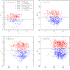Fig. A.1.

Distribution of red galaxies (T_BPZ ≤ 1.5) versus blue galaxies (1.5 < T_BPZ < 3.95) selected according to the photometric type from BPZ and split into different stellar mass bins in g − i versus i colour-magnitude space, as found in the CFHTLenS field W1m0m1. The solid and dotted lines illustrate how we split the lenses into red versus blue bins and approximate stellar mass bins, respectively, in the analysis of CS82 data. The dashed lines additionally indicate g − i limits used to exclude very blue star forming galaxies in the CS82 analysis.

Appendix B: Bayesian estimation of f_h

In Sect. 3.4.3 we described our default analysis approach, where we follow M06 to estimate f_h from the noisy $\hat{Δ Σ_{iso}} (r)$ $\widehat{\Delta \Sigma_{\mathrm{iso}}}(r)$ and $\hat{[f - f_{45}] Δ Σ_{iso} (r)}$ $\widehat{\left[f-f_{45}\right]\Delta \Sigma_{\mathrm{iso}}(r)}$ ¹⁷ estimates in individual radial bins. In this appendix we explore an alternative Bayesian inference approach. Here we first employ the $\hat{Δ Σ_{iso}} (r)$ $\widehat{\Delta \Sigma_{\mathrm{iso}}}(r)$ profile to constrain the posterior probability distribution for the effective mean halo mass M_200c of the particular lens sample

$\begin{matrix} P (M_{200 c} | \hat{Δ Σ_{iso}} (r)) \propto P_{0} (M_{200 c}) P (\hat{Δ Σ_{iso}} (r) | M_{200 c}) \\ \propto P_{0} (M_{200 c}) exp [- \frac{1}{2} \sum_{i} {(\frac{{\hat{Δ Σ}}_{iso} (r_{i}) - Δ Σ_{iso}^{model} (r_{i} | M_{200 c})}{σ_{{\hat{Δ Σ}}_{iso}} (r_{i})})}^{2}], \end{matrix}$ $\begin{aligned}&P\left(M_{\rm 200c}|\,\widehat{\Delta \Sigma _{\rm iso}}(r)\right) \propto P_0(M_{\rm 200c}) P\left(\widehat{\Delta \Sigma _{\rm iso}}(r)|M_{\rm 200c}\right) \nonumber \\&\qquad \propto P_0(M_{\rm 200c}) \exp {\left[-\frac{1}{2}\sum _i\left(\frac{\widehat{\Delta \Sigma }_{\rm iso}(r_i)-\Delta \Sigma _{\rm iso}^\mathrm{model}(r_i|M_{\rm 200c})}{\sigma _{\widehat{\Delta \Sigma }_{\rm iso}}(r_i)}\right)^2\right]}, \end{aligned}$ (B.1)

where we assume a Gaussian likelihood, employ a flat prior in halo mass P₀(M_200c), and ignore the small and noisy off-diagonal elements of the shape-noise-dominated covariance matrix as done in the equations below¹⁸. In Eq. (B.1) the sum runs over all radial bins i with 45 kpc/h₇₀ < r_i < 200 kpc/h₇₀, matching the fit range used in Sect. 4 to constrain halo masses.

We then compute the posterior probability distribution for f_h given the data for this lens bin

$\begin{matrix} P (f_{h} | data) \propto P_{0} (f_{h}) P (data | f_{h}) \\ \propto P_{0} (f_{h}) \int d M_{200 c} P (M_{200 c} | \hat{Δ Σ_{iso}} (r)) P (\hat{[f - f_{45}] Δ Σ_{iso} (r)} | f_{h}, M_{200 c}) \\ \propto P_{0} (f_{h}) \int d M_{200 c} P (M_{200 c} | \hat{Δ Σ_{iso}} (r)) exp [- \frac{1}{2} \sum_{j} χ_{j}^{2}], \end{matrix}$ $\begin{aligned}&P\left(f_{\rm h}|\,\mathrm{data}\right) \propto P_0(f_{\rm h})\, P\left(\mathrm{data}|\,f_{\rm h}\right)\nonumber \\&\quad \propto P_0(f_{\rm h}) \int \mathrm{d} M_{\rm 200c} P\left(M_{\rm 200c}|\widehat{\Delta \Sigma _{\rm iso}}(r)\right) P\left( \widehat{\left[f -f_{45} \right]\Delta \Sigma _{\rm iso}(r)} | f_{\rm h}, M_{\rm 200c}\right)\nonumber \\&\quad \propto P_0(f_{\rm h}) \int \mathrm{d} M_{\rm 200c} P\left(M_{\rm 200c}|\widehat{\Delta \Sigma _{\rm iso}}(r)\right) \exp {\left[-\frac{1}{2} \sum _j \chi ^2_j \right]}, \end{aligned}$ (B.2)

where

$\begin{matrix} χ_{j} = \frac{\hat{[f - f_{45}] Δ Σ_{iso} (r_{j})} - [f_{rel} (r_{j}) - f_{rel, 45} (r_{j})] f_{h} Δ Σ_{iso}^{model} (r_{j} | M_{200 c})}{σ_{\hat{[f - f_{45}] Δ Σ_{iso}}} (r_{j})} \cdot \end{matrix}$ $\begin{aligned} \chi _j= \frac{\widehat{\left[f -f_{45} \right]\Delta \Sigma _{\rm iso}(r_j)} - \left[f_{\rm rel}(r_j)-f_{\rm rel,45}(r_j)\right] f_{\rm h} \Delta \Sigma _{\rm iso}^\mathrm{model}(r_j|M_{\rm 200c})}{\sigma _{\widehat{\left[f -f_{45} \right]\Delta \Sigma _{\rm iso}}}(r_j)}\cdot \end{aligned}$ (B.3)

In Eq. (B.2) we marginalise over halo mass and assume a flat prior P₀(f_h). The factor [f_rel(r_j)−f_rel, 45(r_j)] in Eq. (B.3) also depends on halo mass given its dependence on r/r_s(M_200c) (see Sect. 3.4.2). However, since this dependence is weak (as indicated by the almost flat curves in Fig. 3), and given that the halo masses are well constrained for all of our lens samples (when combining the different lens redshift slices), we can safely employ the [f_rel(r_j)−f_rel, 45(r_j)] model prediction computed at the best-fitting halo mass. Likewise, we keep the fit range 45 kpc/ $h_{70} < r_{j} < r_{200 c}^{best - fit}$ $h_{70} < r_j < r_{200\mathrm{c}}^{\mathrm{best-fit}}$ and therefore the contributing bins j in Eq. (B.3) fixed, as defined by the best-fitting halo mass for this lens sample.

Figure B.1 compares the Bayesian estimates of f_h to the constraints derived from our default analysis for the different lens samples and surveys. We generally find very good agreement between the estimates, confirming the previously employed approach. We note that we do not expect perfect agreement for multiple reasons. For example, our Bayesian approach assumes that the isotropic signal is perfectly modelled by the reduced shear profile of a spherical NFW halo. This is not strictly required for the approach described in Sect. 3.4.3, since it directly uses the $\hat{Δ Σ_{iso}} (r)$ $\widehat{\Delta \Sigma_{\mathrm{iso}}}(r)$ and $\hat{[f - f_{45}] Δ Σ_{iso} (r)}$ $\widehat{\left[f-f_{45}\right]\Delta \Sigma_{\mathrm{iso}}(r)}$ estimates in the same radial bins without explicitly assuming a mass model (of course, both approaches rely on accurate predictions for [f_rel(r)−f_rel, 45(r)], which would change for different density profiles). Likewise, contributions from individual radial bins are weighted differently and change because of the differences between the $\hat{Δ Σ_{iso}} (r_{i})$ $\widehat{\Delta \Sigma_{\mathrm{iso}}}(r_i)$ and $Δ Σ_{iso}^{model} (r_{i})$ $\Delta \Sigma_{\mathrm{iso}}^{\mathrm{model}}(r_i)$ . Finally, the $Δ Σ_{iso}^{model} (r)$ $\Delta \Sigma_{\mathrm{iso}}^{\mathrm{model}}(r)$ model is typically constrained over a fit range with a different upper limit compared to the range used to constrain f_h.

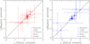Fig. B.1.

Comparison of f_h estimates for the different surveys and lens stellar mass bins from our default analysis scheme (see Sect. 3.4.3) and the Bayesian estimation described in Appendix B. Left and right panels: red and blue lens samples, respectively.

Multiplying the P(f_h| data) posterior probability distributions computed for the individual surveys and different lens bins we can directly compute joint constraints, which are shown in Fig. B.2 for all red and all blue lens samples, respectively. From this we estimate the mode of the distribution and 68% confidence intervals of f_h = 0.268 ± 0.070 for all red lenses, which is in good agreement with the $f_{h} = 0 . 303_{- 0.079}^{+ 0.080}$ $f_{\mathrm{h}}=0.303^{+0.080}_{-0.079}$ constraint derived using our default analysis (see Table 2). We suspect that the slightly smaller error-bars found in the Bayesian analysis may result from the stronger assumptions made in this approach (see above). We note that the significance of the ‘detection’ of a non-zero f_h is basically identical for both approaches (3.8σ). For the blue lens samples the Bayesian approach yields a joint constraint $f_{h} = 0 . 317_{- 0.140}^{+ 0.142}$ $f_{\mathrm{h}}=0.317^{+0.142}_{-0.140}$ , which again has moderately smaller error-bars than the constraint derived using our standard approach ( $f_{h} = 0 . 217_{- 0.159}^{+ 0.160}$ $f_{\mathrm{h}}=0.217^{+0.160}_{-0.159}$ ). For the Bayesian analysis the mode estimate is also noticeably higher than the best-fitting estimate of the default analysis (by 0.6σ using the error of the default analysis), which we suspect may be caused by a combination of the effects discussed above. We suggest that future studies of larger samples could also employ both analysis approaches to investigate if similar shifts are found at a higher significance, which could hint at relevant systematic differences between the constraints derived from both approaches.

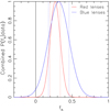Fig. B.2.

Posterior probability distribution (curves, normalised based on the peak value) of f_h for red and blue lenses, combining all surveys and stellar mass bins. The 68% confidence limits are indicated by the vertical dotted lines.

Appendix C: Detailed results for the different surveys

We show the measured isotropic $\hat{Δ Σ} (r)$ $\widehat{\Delta \Sigma}(r)$ and anisotropic $\hat{[f (r) - f_{45} (r)] Δ Σ_{iso} (r)}$ $\widehat{\left[f(r)-f_{45}(r)\right]\Delta \Sigma_{\mathrm{iso}}(r)}$ profiles for CS82, KV450, CFHTLenS, and RCSLenS in Figs. C.1–C.4. The constraints for CFHTLenS differ slightly (well within the error-bars) from the results reported by S15, which is caused by our inclusion of source galaxies with z_b > 1.3.

Fig. C.1.

As Fig. 1, but computed from the KV450 data.

Fig. C.2.

As Fig. 1, but computed from the CFHTLenS data.

Fig. C.3.

As Fig. 1, but computed from the CS82 data.

Fig. C.4.

As Fig. 1, but computed from the RCSLenS data and showing only red lenses.

All Tables

Table 1.

Lens galaxy samples.

In the text

Table 2.

Weak lensing constraints for the different stellar mass and colour bins in the different surveys, as well as joint f_h constraints.

In the text

All Figures

Fig. 1.

Measured isotropic (top sub-panel in each panel) and anisotropic (bottom sub-panel in each panel, note the varying y-axis scale) shear signal around red (left) and blue (right) lenses in the NGVSLenS fields. From top to bottom: decreasing stellar mass bins as indicated. For better readability the anisotropic signal has been scaled by r. The best-fitting NFW shear profile constrained within 45 kpc/h₇₀ < r < 200 kpc/h₇₀ is shown by the curve for the isotropic signal. For (f − f₄₅)ΔΣ the curves show models computed from the best-fit isotropic model and the best-fit f_h for the solid curve, and f_h ∈ { + 1, 0, −1} for the dotted curves, respectively. The best-fit f_h has been constrained from (f − f₄₅)ΔΣ and ΔΣ within 45 kpc/h₇₀ < r < r_200c (range indicated by vertical lines), where r_200c has been estimated from the isotropic signal. The corresponding figures for the other surveys are shown in Appendix C.

In the text

Fig. 2.

Constraints on f_h and M_200c from the different surveys for red (left) and blue (right) lenses. For each survey, the different data points correspond to the different stellar mass bins. The horizontal solid and dotted lines mark the best-fit joint f_h constraints and the ±1σ limits, respectively. For comparison we also show results from the KiDS-1000 analysis of central galaxies from Georgiou et al. (2019b), including their default constraints and their results achieved using a wider weight function for the shape measurements (shown with an offset in mass for clarity).

In the text

Fig. 3.

Ratio of the measured (f − f₄₅)ΔΣ(r) profiles and the best-fit models for the spherical ΔΣ(r) profiles as a function of the radius in units of the NFW scale radius r_s. Left panel: red lenses, while blue lenses are shown on the right. Each grey point corresponds to one data point from Figs. 1 and C.1–C.4 (if it is located within the included fit range, see Sect. 4). Binned averages of these points are shown in black. The curves show model predictions (f_rel − f_rel, 45)f_h for the best-fit joint f_h estimates for all red lenses (left) and all blue lenses (right).

In the text

Fig. 4.

Comparison of constraints on ⟨|ϵ_h|⟩ for red galaxies, galaxy groups, and galaxy clusters from different studies. For our study we combine the constraints from all red lens samples for our two highest stellar mass bins, showing both the uncorrected estimate (assuming perfect alignment of galaxies and haloes), and the more realistic misalignment-corrected estimate. The latter assumes that the impact of misalignment is correctly described by the comparison of the results from the S15 Millennium Simulation analyses with and without misalignment (see Sect. 5). The horizontal error-bars indicate the approximate lens mass range for our results as well as the studies from Oguri et al. (2012), Shin et al. (2018) and Umetsu et al. (2018). For van Uitert et al. (2017) the data point is shown at their best-fit mean mass, where the error corresponds to the fit uncertainty. Clampitt & Jain (2016) only report an approximate mean mass for their sample. We apply mass conversions in case authors employ other definitions than M_200c.

In the text

Fig. A.1.

Distribution of red galaxies (T_BPZ ≤ 1.5) versus blue galaxies (1.5 < T_BPZ < 3.95) selected according to the photometric type from BPZ and split into different stellar mass bins in g − i versus i colour-magnitude space, as found in the CFHTLenS field W1m0m1. The solid and dotted lines illustrate how we split the lenses into red versus blue bins and approximate stellar mass bins, respectively, in the analysis of CS82 data. The dashed lines additionally indicate g − i limits used to exclude very blue star forming galaxies in the CS82 analysis.

In the text

	Fig. B.1. Comparison of f_h estimates for the different surveys and lens stellar mass bins from our default analysis scheme (see Sect. 3.4.3) and the Bayesian estimation described in Appendix B. Left and right panels: red and blue lens samples, respectively.
In the text

	Fig. B.2. Posterior probability distribution (curves, normalised based on the peak value) of f_h for red and blue lenses, combining all surveys and stellar mass bins. The 68% confidence limits are indicated by the vertical dotted lines.
In the text

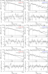	Fig. C.1. As Fig. 1, but computed from the KV450 data.
In the text

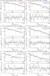	Fig. C.2. As Fig. 1, but computed from the CFHTLenS data.
In the text

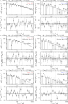	Fig. C.3. As Fig. 1, but computed from the CS82 data.
In the text

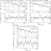	Fig. C.4. As Fig. 1, but computed from the RCSLenS data and showing only red lenses.
In the text

Current usage metrics show cumulative count of Article Views (full-text article views including HTML views, PDF and ePub downloads, according to the available data) and Abstracts Views on Vision4Press platform.

Data correspond to usage on the plateform after 2015. The current usage metrics is available 48-96 hours after online publication and is updated daily on week days.

Initial download of the metrics may take a while.

[1] Adelman-McCarthy, J. K., Agüeros, M. A., Allam, S. S., et al. 2007, ApJS, 172, 634 [NASA ADS] [CrossRef] [Google Scholar]

[2] Adhikari, S., Chue, C. Y. R., & Dalal, N. 2015, JCAP, 1, 9 [Google Scholar]

[3] Agustsson, I., & Brainerd, T. G. 2010, ApJ, 709, 1321 [NASA ADS] [CrossRef] [Google Scholar]

[4] Annis, J., Soares-Santos, M., Strauss, M. A., et al. 2014, ApJ, 794, 120 [NASA ADS] [CrossRef] [Google Scholar]

[5] Arnouts, S., Cristiani, S., Moscardini, L., et al. 1999, MNRAS, 310, 540 [NASA ADS] [CrossRef] [Google Scholar]

[6] Asgari, M., Tröster, T., Heymans, C., et al. 2020, A&A, 634, A127 [NASA ADS] [CrossRef] [EDP Sciences] [Google Scholar]

[7] Bailin, J., & Steinmetz, M. 2005, ApJ, 627, 647 [Google Scholar]

[8] Bartelmann, M., & Schneider, P. 2001, Phys. Rep., 340, 291 [NASA ADS] [CrossRef] [Google Scholar]

[9] Bate, J., Chisari, N. E., Codis, S., et al. 2020, MNRAS, 491, 4057 [Google Scholar]

[10] Begeman, K., Belikov, A. N., Boxhoorn, D. R., & Valentijn, E. A. 2013, Exp. Astron., 35, 1 [NASA ADS] [Google Scholar]

[11] Bekenstein, J. D. 2004, Phys. Rev. D, 70, 083509 [Google Scholar]

[12] Benítez, N. 2000, ApJ, 536, 571 [Google Scholar]

[13] Bertin, E., & Arnouts, S. 1996, A&AS, 117, 393 [NASA ADS] [CrossRef] [EDP Sciences] [Google Scholar]

[14] Bett, P. 2012, MNRAS, 420, 3303 [NASA ADS] [CrossRef] [Google Scholar]

[15] Bett, P., Eke, V., Frenk, C. S., Jenkins, A., & Okamoto, T. 2010, MNRAS, 404, 1137 [NASA ADS] [Google Scholar]

[16] Bhowmick, A. K., Chen, Y., Tenneti, A., Di Matteo, T., & Mandelbaum, R. 2020, MNRAS, 491, 4116 [Google Scholar]

[17] Bliss, C. I. 1935a, Ann. Appl. Biol., 22, 134 [CrossRef] [Google Scholar]

[18] Bliss, C. I. 1935b, Ann. Appl. Biol., 22, 307 [Google Scholar]

[19] Brainerd, T. G., & Wright, C. O. 2000, ArXiv e-prints [arXiv:astro-ph/0006281] [Google Scholar]

[20] Brammer, G. B., van Dokkum, P. G., & Coppi, P. 2008, ApJ, 686, 1503 [NASA ADS] [CrossRef] [Google Scholar]

[21] Bridle, S., & Abdalla, F. B. 2007, ApJ, 655, L1 [NASA ADS] [CrossRef] [Google Scholar]

[22] Bridle, S., & King, L. 2007, New J. Phys., 9, 444 [NASA ADS] [CrossRef] [Google Scholar]

[23] Bruderer, C., Read, J. I., Coles, J. P., et al. 2016, MNRAS, 456, 870 [Google Scholar]

[24] Bundy, K., Leauthaud, A., Saito, S., et al. 2015, ApJS, 221, 15 [NASA ADS] [CrossRef] [Google Scholar]

[25] Bundy, K., Leauthaud, A., Saito, S., et al. 2017, ApJ, 851, 34 [Google Scholar]

[26] Caminha, G. B., Grillo, C., Rosati, P., et al. 2016, A&A, 587, A80 [NASA ADS] [CrossRef] [EDP Sciences] [Google Scholar]

[27] Caminha, G. B., Rosati, P., Grillo, C., et al. 2019, A&A, 632, A36 [CrossRef] [EDP Sciences] [Google Scholar]

[28] Chisari, N. E., Koukoufilippas, N., Jindal, A., et al. 2017, MNRAS, 472, 1163 [Google Scholar]

[29] Choi, A., Heymans, C., Blake, C., et al. 2016, MNRAS, 463, 3737 [NASA ADS] [CrossRef] [Google Scholar]

[30] Chua, K. T. E., Pillepich, A., Vogelsberger, M., & Hernquist, L. 2019, MNRAS, 484, 476 [CrossRef] [Google Scholar]

[31] Clampitt, J., & Jain, B. 2016, MNRAS, 457, 4135 [NASA ADS] [CrossRef] [Google Scholar]

[32] Codis, S., Jindal, A., Chisari, N. E., et al. 2018, MNRAS, 481, 4753 [CrossRef] [Google Scholar]

[33] Coe, D., Benítez, N., Sánchez, S. F., et al. 2006, AJ, 132, 926 [NASA ADS] [CrossRef] [Google Scholar]

[34] Crain, R. A., Theuns, T., Dalla Vecchia, C., et al. 2009, MNRAS, 399, 1773 [NASA ADS] [CrossRef] [Google Scholar]

[35] de Jong, J. T. A., Verdoes Kleijn, G. A., Erben, T., et al. 2017, A&A, 604, A134 [NASA ADS] [CrossRef] [EDP Sciences] [Google Scholar]

[36] Deason, A. J., McCarthy, I. G., Font, A. S., et al. 2011, MNRAS, 415, 2607 [NASA ADS] [CrossRef] [Google Scholar]

[37] Debattista, V. P., van den Bosch, F. C., Roškar, R., et al. 2015, MNRAS, 452, 4094 [Google Scholar]

[38] Despali, G., Giocoli, C., & Tormen, G. 2014, MNRAS, 443, 3208 [NASA ADS] [CrossRef] [Google Scholar]

[39] Despali, G., Giocoli, C., Bonamigo, M., Limousin, M., & Tormen, G. 2017, MNRAS, 466, 181 [NASA ADS] [CrossRef] [Google Scholar]

[40] Diego, J. M., Broadhurst, T., Benitez, N., Lim, J., & Lam, D. 2015, MNRAS, 449, 588 [Google Scholar]

[41] Duffy, A. R., Schaye, J., Kay, S. T., & Dalla Vecchia, C. 2008, MNRAS, 390, L64 [NASA ADS] [CrossRef] [Google Scholar]

[42] Dvornik, A., Zoutendijk, S. L., Hoekstra, H., & Kuijken, K. 2019, A&A, 627, A74 [CrossRef] [EDP Sciences] [Google Scholar]

[43] Erben, T., Hildebrandt, H., Lerchster, M., et al. 2009, A&A, 493, 1197 [NASA ADS] [CrossRef] [EDP Sciences] [Google Scholar]

[44] Erben, T., Hildebrandt, H., Miller, L., et al. 2013, MNRAS, 433, 2545 [Google Scholar]

[45] Evans, A. K. D., & Bridle, S. 2009, ApJ, 695, 1446 [NASA ADS] [CrossRef] [EDP Sciences] [Google Scholar]

[46] Fenech Conti, I., Herbonnet, R., Hoekstra, H., et al. 2017, MNRAS, 467, 1627 [NASA ADS] [Google Scholar]

[47] Ferrarese, L., Côté, P., Cuillandre, J. C., et al. 2012, ApJS, 200, 4 [NASA ADS] [CrossRef] [Google Scholar]

[48] Fieller, E. C. 1954, J. R. Stat. Soc. B, 16, 175 [Google Scholar]

[49] Georgiou, C., Chisari, N. E., Fortuna, M. C., et al. 2019a, A&A, 628, A31 [EDP Sciences] [Google Scholar]

[50] Georgiou, C., Hoekstra, H., Kuijken, K., et al. 2019b, A&A, submitted [Google Scholar]

[51] Gilbank, D. G., Gladders, M. D., Yee, H. K. C., & Hsieh, B. C. 2011, AJ, 141, 94 [NASA ADS] [CrossRef] [Google Scholar]

[52] Hamana, T., Shirasaki, M., Miyazaki, S., et al. 2020, PASJ, 72, 16 [CrossRef] [Google Scholar]

[53] Hand, N., Leauthaud, A., Das, S., et al. 2015, Phys. Rev. D, 91, 062001 [CrossRef] [Google Scholar]

[54] Harvey, D., Tam, S. I., Jauzac, M., Massey, R., & Rhodes, J. 2019, MNRAS, submitted [arXiv:1911.06333] [Google Scholar]

[55] Hayashi, K., & Chiba, M. 2014, ApJ, 789, 62 [Google Scholar]

[56] Hellwing, W. A., Cautun, M., Knebe, A., Juszkiewicz, R., & Knollmann, S. 2013, JCAP, 2013, 012 [CrossRef] [Google Scholar]

[57] Heymans, C., Van Waerbeke, L., Bacon, D., et al. 2006a, MNRAS, 368, 1323 [NASA ADS] [CrossRef] [Google Scholar]

[58] Heymans, C., White, M., Heavens, A., Vale, C., & van Waerbeke, L. 2006b, MNRAS, 371, 750 [NASA ADS] [CrossRef] [Google Scholar]

[59] Heymans, C., Van Waerbeke, L., Miller, L., et al. 2012, MNRAS, 427, 146 [NASA ADS] [CrossRef] [Google Scholar]

[60] Heymans, C., Grocutt, E., Heavens, A., et al. 2013, MNRAS, 432, 2433 [NASA ADS] [CrossRef] [Google Scholar]

[61] Hilbert, S., Hartlap, J., White, S. D. M., & Schneider, P. 2009, A&A, 499, 31 [NASA ADS] [CrossRef] [EDP Sciences] [Google Scholar]

[62] Hilbert, S., Xu, D., Schneider, P., et al. 2017, MNRAS, 468, 790 [Google Scholar]

[63] Hildebrandt, H., Erben, T., Kuijken, K., et al. 2012, MNRAS, 421, 2355 [Google Scholar]

[64] Hildebrandt, H., Choi, A., Heymans, C., et al. 2016, MNRAS, 463, 635 [NASA ADS] [CrossRef] [Google Scholar]

[65] Hildebrandt, H., Viola, M., Heymans, C., et al. 2017, MNRAS, 465, 1454 [Google Scholar]

[66] Hildebrandt, H., Köhlinger, F., van den Busch, J. L., et al. 2020, A&A, 633, A69 [NASA ADS] [CrossRef] [EDP Sciences] [Google Scholar]

[67] Hirata, C. M., & Seljak, U. 2004, Phys. Rev. D, 70, 063526 [NASA ADS] [CrossRef] [Google Scholar]

[68] Hoekstra, H., Franx, M., Kuijken, K., & Squires, G. 1998, ApJ, 504, 636 [NASA ADS] [CrossRef] [Google Scholar]

[69] Hoekstra, H., Franx, M., & Kuijken, K. 2000, ApJ, 532, 88 [NASA ADS] [CrossRef] [Google Scholar]

[70] Hoekstra, H., Yee, H. K. C., & Gladders, M. D. 2004, ApJ, 606, 67 [NASA ADS] [CrossRef] [Google Scholar]

[71] Huang, H.-J., Mandelbaum, R., Freeman, P. E., et al. 2016, MNRAS, 463, 222 [NASA ADS] [CrossRef] [Google Scholar]

[72] Ilbert, O., Arnouts, S., McCracken, H. J., et al. 2006, A&A, 457, 841 [NASA ADS] [CrossRef] [EDP Sciences] [Google Scholar]

[73] Jauzac, M., Harvey, D., & Massey, R. 2018, MNRAS, 477, 4046 [NASA ADS] [CrossRef] [Google Scholar]

[74] Jee, M. J., Tyson, J. A., Hilbert, S., et al. 2016, ApJ, 824, 77 [NASA ADS] [CrossRef] [Google Scholar]

[75] Jing, Y. P., & Suto, Y. 2002, ApJ, 574, 538 [NASA ADS] [CrossRef] [Google Scholar]

[76] Joachimi, B., Semboloni, E., Hilbert, S., et al. 2013a, MNRAS, 436, 819 [Google Scholar]

[77] Joachimi, B., Semboloni, E., Bett, P. E., et al. 2013b, MNRAS, 431, 477 [NASA ADS] [CrossRef] [Google Scholar]

[78] Joachimi, B., Cacciato, M., Kitching, T. D., et al. 2015, Space Sci. Rev., 193, 1 [NASA ADS] [CrossRef] [Google Scholar]

[79] Kacprzak, T., Zuntz, J., Rowe, B., et al. 2012, MNRAS, 427, 2711 [NASA ADS] [CrossRef] [Google Scholar]

[80] Kaiser, N. 1995, ApJ, 439, L1 [NASA ADS] [CrossRef] [Google Scholar]

[81] Kaiser, N., Squires, G., & Broadhurst, T. 1995, ApJ, 449, 460 [NASA ADS] [CrossRef] [Google Scholar]

[82] Kannawadi, A., Hoekstra, H., Miller, L., et al. 2019, A&A, 624, A92 [NASA ADS] [CrossRef] [EDP Sciences] [Google Scholar]

[83] Khoperskov, S. A., Moiseev, A. V., Khoperskov, A. V., & Saburova, A. S. 2014, MNRAS, 441, 2650 [NASA ADS] [CrossRef] [Google Scholar]

[84] Kitching, T. D., Miller, L., Heymans, C. E., van Waerbeke, L., & Heavens, A. F. 2008, MNRAS, 390, 149 [NASA ADS] [CrossRef] [Google Scholar]

[85] Kuijken, K., Heymans, C., Hildebrandt, H., et al. 2015, MNRAS, 454, 3500 [Google Scholar]

[86] Kuijken, K., Heymans, C., Dvornik, A., et al. 2019, A&A, 625, A2 [NASA ADS] [CrossRef] [EDP Sciences] [Google Scholar]

[87] Laigle, C., Pichon, C., Codis, S., et al. 2015, MNRAS, 446, 2744 [NASA ADS] [CrossRef] [Google Scholar]

[88] Laureijs, R., Amiaux, J., Arduini, S., et al. 2011, ArXiv e-prints [arXiv:1110.3193] [Google Scholar]

[89] Leauthaud, A., Saito, S., Hilbert, S., et al. 2017, MNRAS, 467, 3024 [NASA ADS] [CrossRef] [Google Scholar]

[90] L’Huillier, B., Winther, H. A., Mota, D. F., Park, C., & Kim, J. 2017, MNRAS, 468, 3174 [NASA ADS] [CrossRef] [Google Scholar]

[91] Limousin, M., Morandi, A., Sereno, M., et al. 2013, Space Sci. Rev., 177, 155 [NASA ADS] [CrossRef] [Google Scholar]

[92] Liu, X., Pan, C., Li, R., et al. 2015, MNRAS, 450, 2888 [NASA ADS] [CrossRef] [Google Scholar]

[93] LSST Science Collaboration (Abell, P. A., et al.) 2009, ArXiv e-prints [arXiv:0912.0201] [Google Scholar]

[94] Luppino, G. A., & Kaiser, N. 1997, ApJ, 475, 20 [NASA ADS] [CrossRef] [Google Scholar]

[95] Mandelbaum, R., Hirata, C. M., Broderick, T., Seljak, U., & Brinkmann, J. 2006, MNRAS, 370, 1008 [NASA ADS] [CrossRef] [Google Scholar]

[96] Massey, R., Heymans, C., Bergé, J., et al. 2007, MNRAS, 376, 13 [Google Scholar]

[97] Melchior, P., & Viola, M. 2012, MNRAS, 424, 2757 [Google Scholar]

[98] Melchior, P., Viola, M., Schäfer, B. M., & Bartelmann, M. 2011, MNRAS, 412, 1552 [NASA ADS] [CrossRef] [Google Scholar]

[99] Milgrom, M. 1983, ApJ, 270, 365 [NASA ADS] [CrossRef] [Google Scholar]

[100] Milgrom, M. 2001, MNRAS, 326, 1261 [Google Scholar]

[101] Miller, L., Kitching, T. D., Heymans, C., Heavens, A. F., & van Waerbeke, L. 2007, MNRAS, 382, 315 [Google Scholar]

[102] Miller, L., Heymans, C., Kitching, T. D., et al. 2013, MNRAS, 429, 2858 [Google Scholar]

[103] Miralda-Escude, J. 1991, ApJ, 370, 1 [NASA ADS] [CrossRef] [Google Scholar]

[104] Moffat, J. W. 2006, JCAP, 3, 4 [NASA ADS] [CrossRef] [Google Scholar]

[105] Moffat, J. W., & Toth, V. T. 2009, MNRAS, 397, 1885 [NASA ADS] [CrossRef] [Google Scholar]

[106] Natarajan, P., & Refregier, A. 2000, ApJ, 538, L113 [NASA ADS] [CrossRef] [Google Scholar]

[107] Navarro, J. F., Frenk, C. S., & White, S. D. M. 1996, ApJ, 462, 563 [Google Scholar]

[108] Navarro, J. F., Frenk, C. S., & White, S. D. M. 1997, ApJ, 490, 493 [NASA ADS] [CrossRef] [Google Scholar]

[109] Oguri, M., Takada, M., Okabe, N., & Smith, G. P. 2010, MNRAS, 405, 2215 [NASA ADS] [Google Scholar]

[110] Oguri, M., Bayliss, M. B., Dahle, H., et al. 2012, MNRAS, 420, 3213 [NASA ADS] [CrossRef] [Google Scholar]

[111] Okamoto, T., Eke, V. R., Frenk, C. S., & Jenkins, A. 2005, MNRAS, 363, 1299 [NASA ADS] [CrossRef] [Google Scholar]

[112] Okumura, T., Jing, Y. P., & Li, C. 2009, ApJ, 694, 214 [NASA ADS] [CrossRef] [Google Scholar]

[113] Parker, L. C., Hoekstra, H., Hudson, M. J., van Waerbeke, L., & Mellier, Y. 2007, ApJ, 669, 21 [NASA ADS] [CrossRef] [Google Scholar]

[114] Parroni, C., Mei, S., Erben, T., et al. 2017, ApJ, 848, 114 [NASA ADS] [CrossRef] [Google Scholar]

[115] Paterno-Mahler, R., Sharon, K., Coe, D., et al. 2018, ApJ, 863, 154 [Google Scholar]

[116] Peter, A. H. G., Rocha, M., Bullock, J. S., & Kaplinghat, M. 2013, MNRAS, 430, 105 [Google Scholar]

[117] Peters, S. P. C., van der Kruit, P. C., Allen, R. J., & Freeman, K. C. 2017, MNRAS, 464, 65 [Google Scholar]

[118] Piras, D., Joachimi, B., Schäfer, B. M., et al. 2018, MNRAS, 474, 1165 [NASA ADS] [CrossRef] [Google Scholar]

[119] Planck Collaboration VI. 2020, A&A, 641, A6 [NASA ADS] [CrossRef] [EDP Sciences] [Google Scholar]

[120] Raichoor, A., Mei, S., Erben, T., et al. 2014, ApJ, 797, 102 [NASA ADS] [CrossRef] [Google Scholar]

[121] Refregier, A., Kacprzak, T., Amara, A., Bridle, S., & Rowe, B. 2012, MNRAS, 425, 1951 [Google Scholar]

[122] Rykoff, E. S., Rozo, E., Busha, M. T., et al. 2014, ApJ, 785, 104 [NASA ADS] [CrossRef] [Google Scholar]

[123] Schäfer, B. M., & Merkel, P. M. 2017, MNRAS, 470, 3453 [Google Scholar]

[124] Schneider, P., & Watts, P. 2005, A&A, 432, 783 [NASA ADS] [CrossRef] [EDP Sciences] [Google Scholar]

[125] Schneider, P., Kochanek, C., & Wambsganss, J. 2006, in Gravitational Lensing: Strong, Weak & Micro, Saas-Fee Advanced Course 33, eds. G. Meylan, P. Jetzer, & P. North (Berlin: Springer-Verlag), Swiss Soc. Astrophys. Astron. [Google Scholar]

[126] Schrabback, T., Hartlap, J., Joachimi, B., et al. 2010, A&A, 516, A63 [NASA ADS] [CrossRef] [EDP Sciences] [Google Scholar]

[127] Schrabback, T., Hilbert, S., Hoekstra, H., et al. 2015, MNRAS, 454, 1432 [Google Scholar]

[128] Schrabback, T., Applegate, D., Dietrich, J. P., et al. 2018, MNRAS, 474, 2635 [Google Scholar]

[129] Seitz, C., & Schneider, P. 1997, A&A, 318, 687 [NASA ADS] [Google Scholar]

[130] Shan, H. Y., Kneib, J.-P., Comparat, J., et al. 2014, MNRAS, 442, 2534 [Google Scholar]

[131] Shin, T.-H., Clampitt, J., Jain, B., et al. 2018, MNRAS, 475, 2421 [Google Scholar]

[132] Shirasaki, M., & Yoshida, N. 2018, MNRAS, 475, 1665 [Google Scholar]

[133] Simon, P., Schneider, P., & Kübler, D. 2012, A&A, 548, A102 [NASA ADS] [CrossRef] [EDP Sciences] [Google Scholar]

[134] Springel, V., White, S. D. M., Jenkins, A., et al. 2005, Nature, 435, 629 [NASA ADS] [CrossRef] [PubMed] [Google Scholar]

[135] Suyu, S. H., Hensel, S. W., McKean, J. P., et al. 2012, ApJ, 750, 10 [NASA ADS] [CrossRef] [Google Scholar]

[136] Tenneti, A., Mandelbaum, R., Di Matteo, T., Feng, Y., & Khandai, N. 2014, MNRAS, 441, 470 [NASA ADS] [CrossRef] [Google Scholar]

[137] Tenneti, A., Mandelbaum, R., & Di Matteo, T. 2016, MNRAS, 462, 2668 [NASA ADS] [CrossRef] [Google Scholar]

[138] Troxel, M. A., MacCrann, N., Zuntz, J., et al. 2018, Phys. Rev. D, 98, 043528 [Google Scholar]

[139] Tugendhat, T. M., & Schäfer, B. M. 2018, MNRAS, 476, 3460 [Google Scholar]

[140] Umetsu, K. 2020, A&ARv, 28, 7 [Google Scholar]

[141] Umetsu, K., Sereno, M., Tam, S.-I., et al. 2018, ApJ, 860, 104 [NASA ADS] [CrossRef] [Google Scholar]

[142] van Uitert, E., Hoekstra, H., Schrabback, T., et al. 2012, A&A, 545, A71 [NASA ADS] [CrossRef] [EDP Sciences] [Google Scholar]

[143] van Uitert, E., Hoekstra, H., Joachimi, B., et al. 2017, MNRAS, 467, 4131 [NASA ADS] [CrossRef] [Google Scholar]

[144] Vega-Ferrero, J., Yepes, G., & Gottlöber, S. 2017, MNRAS, 467, 3226 [Google Scholar]

[145] Velander, M., van Uitert, E., Hoekstra, H., et al. 2014, MNRAS, 437, 2111 [NASA ADS] [CrossRef] [Google Scholar]

[146] Velliscig, M., Cacciato, M., Schaye, J., et al. 2015, MNRAS, 453, 721 [NASA ADS] [CrossRef] [Google Scholar]

[147] Wright, C. O., & Brainerd, T. G. 2000, ApJ, 534, 34 [NASA ADS] [CrossRef] [Google Scholar]

[148] Wright, A. H., Hildebrandt, H., Kuijken, K., et al. 2019, A&A, 632, A34 [NASA ADS] [CrossRef] [EDP Sciences] [Google Scholar]

Tightening weak lensing constraints on the ellipticity of galaxy-scale dark matter haloes

1. Introduction

2. Data

2.1. CFHTLenS

2.2. RCSLenS

2.3. NGVSLenS

2.4. CS82

2.5. KiDS/KV450

3. Analysis

3.1. Shape measurements for bright galaxies

3.2. Lens galaxies

3.3. Source sample

3.4. Extracting the weak lensing halo shape signature

3.4.1. Constraining the isotropic shear field

3.4.2. Constraining the anisotropic shear field

3.4.3. Estimating fh

4. Results

5. Discussion

6. Conclusions

Acknowledgments

References

Appendix A: Lens sub-samples in CS82

Appendix B: Bayesian estimation of fh

Appendix C: Detailed results for the different surveys

All Tables

All Figures

3.4.3. Estimating f_h

Appendix B: Bayesian estimation of f_h