| Issue |
A&A
Volume 645, January 2021
|
|
|---|---|---|
| Article Number | A95 | |
| Number of page(s) | 22 | |
| Section | Catalogs and data | |
| DOI | https://doi.org/10.1051/0004-6361/202039476 | |
| Published online | 19 January 2021 | |
The ROSAT Raster survey in the north ecliptic pole field
X-ray catalogue and optical identifications⋆
1
European Space Astronomy Centre (ESA/ESAC), 28691 Villanueva de la Cañada, Madrid, Spain
e-mail: This email address is being protected from spambots. You need JavaScript enabled to view it.
2
Institute for Astronomy, University of Hawaii, 2680 Woodlawn Drive, Honolulu, HI 96822, USA
3
Max-Planck-Institut für Extraterrestrische Physik, Giessenbachstrasse 1, 85748 Garching, Germany
4
Department of Astrophysical Sciences, Princeton University, 4 Ivy Lane, Princeton, NJ 08544, USA
5
Infrared Processing and Analysis Center (IPAC), 1200 East California Boulevard, Pasadena, California 91125, USA
6
California Institute of Technology, 1200 East California Boulevard, Pasadena, California 91125, USA
7
Institut d’Astrophysique de Paris, CNRS (UMR7095), 98 Bis Boulevard Arago, 75014 Paris, France
Received:
20
September
2020
Accepted:
9
November
2020
Abstract
The north ecliptic pole (NEP) is an important region for extragalactic surveys. Deep and wide contiguous surveys are being performed by several space observatories, most currently with the eROSITA telescope. Several more are planned for the near future. We analyse all the ROSAT pointed and survey observations in a region of 40 deg2 around the NEP, restricting the ROSAT field of view to the inner 30′ radius. We obtain an X-ray catalogue of 805 sources with 0.5−2 keV fluxes > 2.9 × 10⁻¹⁵ erg cm−2 s−1, about a factor of three deeper than the ROSAT All-Sky Survey in this field. The sensitivity and angular resolution of our data are comparable to the eROSITA All-Sky Survey expectations. The 50% position error radius of the sample of X-ray sources is ∼10″. We use HEROES optical and near-infrared imaging photometry from the Subaru and Canada/France/Hawaii telescopes together with GALEX, SDSS, Pan-STARRS, and WISE catalogues, as well as images from a new deep and wide Spitzer survey in the field to statistically identify the X-ray sources and to calculate photometric redshifts for the candidate counterparts. In particular, we utilize mid-infrared (mid-IR) colours to identify active galactic nucleus (AGN) X-ray counterparts. Despite the relatively large error circles and often faint counterparts, together with confusion issues and systematic errors, we obtain a rather reliable catalogue of 766 high-quality optical counterparts, corresponding redshifts and optical classifications. The quality of the dataset is sufficient to look at ensemble properties of X-ray source classes. In particular we find a new population of luminous absorbed X-ray AGN at large redshifts, identified through their mid-IR colours. This populous group of AGN was not recognized in previous X-ray surveys, but could be identified in our work due to the unique combination of survey solid angle, X-ray sensitivity, and quality of the multi-wavelength photometry. We also use the WISE and Spitzer photometry to identify a sample of 185 AGN selected purely through their mid-IR colours, most of which are not detected by ROSAT. Their redshifts and upper limits to X-ray luminosity and X-ray–to–optical flux ratios are even higher than for the new class of X-ray selected luminous type 2 AGN (AGN2); they are probably a natural extension of this sample. This unique dataset is important as a reference sample for future deep surveys in the NEP region, in particular for eROSITA and also for Euclid and SPHEREX. We predict that most of the absorbed distant AGN should be readily picked up by eROSITA, but they require sensitive mid-IR imaging to be recognized as optical counterparts.
Key words: surveys / catalogs / galaxies: nuclei / quasars: general / X-rays: galaxies / X-rays: galaxies: clusters
Full Tables 1, 3, and 4 are only available at the CDS via anonymous ftp to cdsarc.u-strasbg.fr (130.79.128.5) or via http://cdsarc.u-strasbg.fr/viz-bin/cat/J/A+A/645/A95
© ESO 2021
1. Introduction
The north ecliptic pole (NEP) region around the coordinates α(2000) = 18h00m00s, δ(2000) = +66°33′39″ is an important area for space-based extragalactic surveys. A number of spacecraft are powered by fixed solar arrays, which need to face towards the sun. This gives them a degree of freedom to point in any direction roughly perpendicular to the sun. The two ecliptic poles, the NEP and also the south ecliptic pole (SEP), are always accessible during the mission, and are thus prime targets for surveys and performance verification or calibration targets. Spacecrafts performing all-sky surveys by continuously scanning the sky perpendicular to the sun accumulate particularly large amounts of exposure time around the ecliptic poles.
The SEP is close to the Small and Large Magellanic Clouds, which limits our visibility to the extragalactic sky; it is thus less suitable. But the NEP is perfectly situated for unbiased deep and wide extragalactic surveys. The ROSAT X-ray observatory performed an all-sky survey (Trümper 1982) perpendicular to the sun–Earth direction and executed a particularly deep and wide survey at the NEP (Henry et al. 2006, hereafter H06) as well as several deep pointings for operational reasons (Hasinger et al. 1991; Bower et al. 1996). The AKARI infrared satellite performed a deep NEP survey (Matsuhara et al. 2006; Goto et al. 2017), which was later followed up by the far-infrared observatory Herschel (Pearson et al. 2019).
Future missions will also have an important focus on the NEP. The eROSITA (Merloni et al. 2012; Predehl et al. 2021) and ART-XC (Pavlinsky et al. 2018) telescopes on board the Spektr-RG mission (Pavlinsky et al. 2009) are currently producing an X-ray all-sky survey more than an order of magnitude deeper than ROSAT, which again will have particularly deep and wide coverage at the ecliptic poles (see Merloni et al. 2020). The future NASA Medium Explorer mission SPHEREx (Korngut et al. 2018; Doré et al. 2018) will perform an all-sky spectroscopic survey in the near-infrared (NIR), again using the sun-perpendicular scanning scheme with particularly deep and wide ecliptic pole surveys. The ESA dark energy survey mission Euclid has selected three Deep Fields, one of which is also centred on the NEP. The James Webb Space Telescope will perform a long-term time-domain survey in its continuous viewing zone field close to the NEP (Jansen & Windhorst 2018), which is also currently monitored with Chandra (Maksym et al. 2019). In preparation for these future surveys we have embarked on the wide-deep UgrizyJ imaging survey HEROES1 with the Subaru and CFHT telescopes on Maunakea, covering about 40 deg2 centred on the NEP (see e.g., Songaila et al. 2018), as well as a deep Spitzer coverage of the Euclid NEP deep field (Moneti et al., in prep.).
In addition to the deep coverage in the all-sky survey and several serendipitous pointings centred on the NEP, ROSAT has also performed a large number of raster-scan pointings around the NEP, as well as several pointed observations on particular interesting targets. The motivation for this work is to analyse all the ROSAT survey and pointing data in the HEROES area in a systematic and coherent fashion. In order to do so, we have restricted the off-axis angle of the ROSAT observations to < 30′ in order to avoid the outer portions of the field of view (FOV), where the point spread function (PSF) degrades significantly. As we show in this paper, the soft X-ray sensitivity limit and the resulting angular resolution of this NEP raster-scan survey can be compared to the expected parameters of the eROSITA all-sky survey, and can thus provide a real-sky approximation and reference field for this ongoing survey. Throughout this work we adopt a Λ-cosmology with ΩM = 0.3 and ΩΛ = 0.7, and H0 = 70 km s−1 Mpc−1 (Spergel et al. 2003), and all magnitudes are given in the AB system.
2. The ROSAT data preparation
Table A.1 shows the observing log of the ROSAT observations within ∼3.5 deg from the NEP used for our analysis. Apart from the ROSAT All-Sky Survey (RASS) there were about 35 raster pointings distributed around the NEP. In addition to the very long ROSAT Wide-Field Camera (WFC) background observations in the beginning of the mission, there were also a number of deep ‘Idle’ or ‘Dummy’ pointings close to the NEP (filling gaps in the observation timeline), plus pointings towards several interesting individual targets in the same region. We note that all observations in 1990 were performed with the primary ROSAT Position Sensitive Proportional Counter (PSPC-C, Pfeffermann et al. 1987), while after an unfortunate incident in which the PSPC-C looked at the sun and was destroyed, the redundant PSPC-B was used. This whole dataset has never been analysed jointly and in a coherent way. For our analysis we used a version of the interactive scientific analysis EXSAS (Zimmermann et al. 1993) system available on a computer at MPE Garching. In general we followed the analysis procedure in H06, which is based on the standard ROSAT data reduction described in detail in Voges et al. (1999). However, we applied a number of non-standard selections and corrections to the data before the actual source detection. We first downloaded all the data listed in Table A.1 and projected the X-ray events and the attitude files to a common celestial reference frame centred on the NEP.
Next we chose an optimum cut-off radius for the detector FOV. The PSPC has a circular FOV with a radius 57′. The PSPC entrance window has a rib support structure with an inner ring at a radius corresponding to 20′ (Pfeffermann et al. 1987; Hasinger & Zamorani 2000). Both the ROSAT telescope angular resolution and its vignetting function are roughly constant within the inner 20′ ring, but degrade significantly towards larger off-axis angles. The combined detector and telescope PSFs are described in detail in Boese (2000). To the first order, the PSF at each off-axis angle can be approximated by a Gaussian function with a half power radius (HPR) of 13, 22, 52, 93, 130, and 180″, at off-axis angles of 0, 12, 24, 36, 48, and 57′, respectively (at 1 keV). The vignetting function at 1 keV drops almost linearly to about 50% at an off-axis angle of 50′. Taking into account all these effects, the HPR of the overall RASS PSF is 84″ (Boese 2000). This means that the classical confusion limit (40 beams per source) is reached at a source density of about 15 sources deg−2, which is exceeded in the high-exposure areas of our survey. In addition, we need to optimally discriminate between extended and point-like X-ray sources, calling for an angular resolution that is as high as possible. We therefore have to reduce the detector FOV. The sharpest imaging is achieved within the inner 20′ of the PSPC FOV, corresponding to the inner ring-like rib of the PSPC support structure (see Fig. 1). However, there is a trade-off between image sharpness and the number of photons required for detection and image characterization. In particular in the outer areas of our survey, where the RASS exposure times drop significantly, a 20′ FOV radius does not provide sufficient exposure time. Taking into account the various competing factors in this trade-off, we made a few tests varying the FOV cut-off radius, and finally decided on an optimum FOV radius of 30′. The PSPC detector coordinates have a pixel size of 0.934″. We thus removed all X-ray events from the dataset, which are further than 1925 pixels from the PSPC centre pixel coordinate [4119,3929]. A similar cut had to be applied to the modified PSPC instrument map (MOIMP), which is used later for the construction of the survey exposure map.
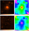 |
Fig. 1. Raw hard-band (0.5−2 keV) image of the NEP raster scan (upper left, scale in raw counts); exposure map (upper right, scale in seconds); exposure-corrected image (lower left, scale in counts s−1); count rate sensitivity map (lower right, scale in counts s−1). The image size is 6.4° ×6.4°, centred on the NEP. The pixel size is 45″. |
Using the information in Boese (2000), we calculated an effective survey PSF by appropriately weighting the corresponding functions at 0, 12, and 24′; this function has an HPR of 34″, i.e. about 2.5 times sharper than the standard RASS PSF, but still about 30% larger than the expected eROSITA survey PSF (Merloni et al. 2012). It should be noted that our survey contains both survey and raster-scan data, for which the PSF approximation averaged over the whole FOV is appropriate. But the survey also contains a number of deep pointed observations of specific targets, for which a local PSF model would be more appropriate. To a large degree the maximum likelihood algorithm discussed below takes care of these differences.
The next step of the analysis is the astrometric correction of the X-ray events to a common reference frame. For this purpose we analysed all the pointed observations in Table A.1 separately, and compared the detected X-ray positions to a catalogue of optical reference point sources from the Gaia DR2 catalogue (Gaia Collaboration 2018). We detected and corrected an offset of 10″ for all pointed observations performed with the PSPC-C, while all PSPC-B observations are compatible (within the errors) with the Gaia reference frame. For the RASS part of the data we cut the survey into ten roughly equal time intervals and detected the X-ray sources in individual images of the central NEP region. All the individual detections are consistent with the average survey image and the Gaia reference frame, so that we did not need to apply an astrometric correction to the survey data.
3. X-ray analysis
3.1. Source detection
We have restricted the basic source detection to the standard hard ROSAT PSPC energy band (0.5−2 keV), corresponding to PSPC PHA channels 52−201. For extragalactic work this is the most sensitive band, least affected by interstellar absorption and also with the best PSPC angular resolution. The interstellar neutral hydrogen column density in our region of interest varies from NH = 2.5 × 10²⁰ to 8.3 × 1020 cm−2 with a median of 4.1 × 1020 cm−2 (Elvis et al. 1994). In the hard band this leads to negligible absorption differences, while in the soft (0.1−0.4 keV) band the variation in transmission would be a factor of 7 across the field.
We accumulated an image in the 0.5−2 keV band centred on the NEP with 512 × 512 pixels of 45″ each. Figure 1 (upper left) shows the resulting raw counts image, where the different exposure times are clearly visible. The image in the upper right of the figure shows the exposure map, calculated from the ROSAT attitude files and the PSPC modified instrument map (MOIMP) representing the detailed geometry of the PSPC support window and the telescope vignetting. Some of the deeper pointings have been carried out in a static (i.e. non-wobbled) observing mode. For these, the structure of the PSPC support window is clearly visible in the exposure map, while it is partly smeared out in the wobbled exposures. The detailed effect of the PSPC support structure and the Wobble-Mode on the ROSAT deep surveys has been discussed in Hasinger & Zamorani (2000). The image on the lower left is the exposure-corrected count rate map. Apart from some enhanced noise artefacts due to the relatively low exposure in the upper left and lower right corners, the image appears quite homogeneous, despite the large variations in exposure time, confirming the quality of the exposure map. Some bright diffuse X-ray sources can be readily identified.
For the source detection we followed the RASS procedure described in Voges et al. (1999) and H06. However, we apply the detection only to the hard-band image, and use the SExtractor (Bertin & Arnouts 1996) detection technique instead of the standard map detection method MDETECT before the final maximum likelihood (ML) source characterization. The first step is the local detection algorithm LDETECT, using a 3 × 3 pixel detect cell, and a local measurement of the background in the surrounding 16 pixels. After a first pass at full resolution, the detect cell and corresponding background area are successively doubled in several more passes in order to also detect larger extended sources. The LDETECT step is applied to the raw image (see Fig. 1, upper left panel) uncorrected for exposure time.
A more elaborate background map is used for the next detection step. Around every X-ray source detected by LDETECT (using a higher likelihood threshold of L ≥ 10) a circular region with a radius about the size of the detect cell is cut out from the raw image (the ‘swiss cheese map’). The remaining image is then divided by the exposure map and binned into coarser pixels. This cleaned, exposure-corrected image is fit by a smooth two-dimensional spline. After the spline fit, a 4σ cut is applied to pixels with count rates above the determined background in order to remove artefacts from large diffuse sources and bright source haloes. This procedure is repeated until no more excess coarse pixels are found. Finally, a background map is produced by applying the spline parameters to all pixels in the original image and multiplying by the exposure map. Figure 1 (lower right) shows the count rate sensitivity map, which is a combination of the background map and the exposure map (see below).
The standard second stage of the source detection using the map detection algorithm MDETECT on the raw image with the same detection cells as LDETECT, but taking the background map estimate instead of the local background, turned out not to be appropriate for our complex set of observations. The standard LDETECT and MDETECT algorithms are not able to accurately model the high-sensitivity confusion-limited areas in the image, and the large exposure gradients and diffuse emission features produce a number of artefacts creating difficulties for the standard detection procedures. We therefore decided to apply the SExtractor algorithm, well known in optical astronomy (Bertin & Arnouts 1996), as the interim detection step offering possible regions of interest to the final ML source detection and characterization. This procedure works reasonably well for isolated point sources, and even moderately confused sources, and for bright diffuse sources. However, it breaks down at the low-exposure regions; in this case Gaussian statistics are no longer appropriate and have to be replaced by Poissonian estimates. This is the reason, why we performed a detailed visual inspection and screening of the SExtractor source list selecting 1200 regions of interest to be finally offered to the ML procedure. In this step we also manually inserted a number of source regions of interest that were missed by the algorithms, which are flagged in the final catalogue.
3.2. The ROSAT NEP Raster Catalogue
The third and last detection step uses a ML algorithm (Cruddace et al. 1988; Boese & Doebereiner 2001) applied to unbinned individual photons to both detect the sources and measure their final parameters. X-ray events in a circle of 3′ radius around every entry in the regions of interest list were selected. For a subset of 34 significantly extended sources (flagged in the final catalogue) we increased the event selection radius to 6′. The ML fit takes into account each photon with the appropriate PSF corresponding to the off-axis angle and energy at which it was detected. An effectively smaller extraction radius and therefore higher weight is given to photons detected near the centre of the field, compared to those at the outskirts with a worse PSF. The ML analysis yields a number of parameters for each source. Most important is the source existence likelihood Lexi = −ln(P0), where P0 is the probability that the source count rate is zero (see Boese & Doebereiner 2001). The threshold for this parameter has been set to Lexi ≥ 11 to define the final content of our survey. The likelihood analysis also determines the best parameters for the source position and a corresponding position error, the net detected counts of the source and its error, and an estimate of the angular extent of the source and the likelihood that it is extended. To estimate this extent the ML algorithm fits a Gaussian model added in quadrature to the PSF.
Table 1 gives the final catalogue of 805 detected X-ray sources in an abbreviated form; the complete catalogue is available at the CDS. For all sources the parameters of the ML analysis are quoted. A threshold of Lexi ≥ 11 has been applied throughout (see below). For a true estimate of source extent, a combination of existence likelihood and extent likelihood have to be considered (see discussion below). In order to convert the source count rates to fluxes, following previous work, we assume an extragalactic point source with a photon index of −2 and an interstellar column density of NH = 4.1 × 1020 cm−2, folded through the PSPC response matrix. A source with a 0.5−2 keV flux of 10−11 erg cm−2 s−1 yields a PSPC count rate of 0.815 cts s−1 in the 0.5−2 keV band. Because we restrict the source detection to the hard band, variations of NH across the field can be neglected. Therefore, the extragalactic point source fluxes can be readily converted into other spectral model fluxes. For 34 sources significantly extended in the first ML analysis or by visual inspection, the extent characterization of the ML algorithm may be insufficient because of the limited photon extraction radius, among other reasons, and therefore the detected count rate could be significantly underestimated. For these sources we determined the ML parameters by doubling the event extraction radius; they are flagged with (1) in Col. (11) of the catalogue. Another ten non-extended sources, which were originally not included in the source region of interest list, were manually fed through the normal ML detection procedure and are also flagged in Col. (11).
ROSAT NEP Raster X-ray Catalogue.
As a final quality check of the source detection we compared our catalogue to previous X-ray information in the HEROES field, predominantly with the second ROSAT all-sky survey (2RXS) source catalogue (Boller et al. 2016) and the second XMM-Newton Slew Survey2 (XMMSL2) (see also Salvato et al. 2018), and with the fourth-generation XMM-Newton serendipitous source catalogue (4XMM-DR9, Webb et al. 2020). A total of 477 of our 805 X-ray sources have counterparts in the literature. In particular there are 431 matches with 2RXS, 83 with 4XMM-DR9, and 40 with XMMSL2. About half of these matches (228) are also present in the H06 catalogue. As expected, the 2RXS analysis has a greater difficulty in determining source extents and resolving confusion, but yields better accuracy for isolated sources in the outskirts of our survey. As we discuss below, the literature data (in particular the better XMM-Newton positions) confirmed almost all of our optical counterparts in the overlapping areas, except for 17 cases identified as high-quality optical counterparts that would have been missed in our analysis.
3.3. Sensitivity limits
An important consideration is the setting of the source detection threshold Lexi and thus the corresponding sensitivity function for the survey. It has to be chosen to maximize the number of true sources in the survey, and to minimize the number of spurious sources. The expected number of spurious sources is the above probability P0 multiplied with the number of statistically independent trials ntrial across the field. Given the rather complex setup of our survey, and the intricacies of the ML source detection algorithm, it is not possible to determine ntrial analytically. A rough estimate is the number of statistically independent detection cells in the LDETECT process, which is (512 × 512)/(3 × 3) = 29127. Below, in the context of calculating the survey sensitivity function, we derive the average effective extraction radius for our ML analysis, which is 1.35 pixels, or 60.8″. Using this number for the size of the detection cell, we arrive at 45785 independent trials. Therefore, an existence likelihood threshold of Lexi ≥ 11 is applied to statistically obtain less than one spurious source in the overall survey. This threshold is more conservative than the limits of Lexi ≥ 6.5 or Lexi ≥ 9, for example, selected for the 2RXS source catalogue (Boller et al. 2016), which lead to a much larger spurious source fraction of about 30% and 5%, respectively. The treatment is, however, rather simplified. In reality, systematic effects can increase the number of spurious sources (e.g., the high diffuse surface brightness around bright extended and point sources discussed above) and the effects of confusion. Using the likelihood threshold of Lexi ≥ 11, we can thus expect a handful of spurious sources, consistent with the optical identifications discussed in Sect. 4.4. Together with a careful manual screening of spurious sources and merging of split source components, we arrive at a catalogue of 805 X-ray sources (see Table 1). A total of 254 of our sources match entries in the H06 catalogue within 2.5σ error circles. These matches are indicated with black solid circles in the relevant figures throughout this paper. The classical confusion limit in radio astronomy is defined as 40 beams (i.e. statistically independent detection cells) per source (Condon 1974). With the number of independent trials estimated above, this corresponds to 1145 sources in the whole survey, or about 28 sources deg−2. Our average source density is below this number, but in the deepest pointed areas around the NEP the source density is higher than this classical confusion limit.
In order to use the survey for quantitative statistics, it is important to calculate a survey selection function. This is equivalent to the sky coverage solid angle, within which sources of a particular brightness would have been detected in the survey. For the ML algorithm described above, with its intricacy of different effective detection cell radii for individual photons, it is not possible to calculate a sensitivity limit analytically. Therefore, some publications resort to extensive Monte Carlo simulations for the determination of the sky coverage function (see e.g., Cappelluti et al. 2009). For the statistical applications in this paper it is appropriate to approximate the sensitivity map by a simple signal-to-noise ratio calculation, following the procedure described in H06. In the case of significant background in the detection cell the likelihood can be approximated by a Gaussian probability distribution. A detection likelihood of Lexi ≥ 11 almost exactly corresponds to a Gaussian probability of 3σ, so we base our sensitivity calculation on this limit. In the background limited case, the signal-to-noise ratio can be calculated as  , where S is the net detected counts of a source, and B is the number of background counts in the source detection cell. For a given background brightness per pixel of b, the background counts in a circular detect cell of radius rb is simply
  . For the purpose of this analysis b is assumed error-free because it has been determined from a large background map with high statistical accuracy.
Compared to the original extraction radius of 3′ for the ML algorithm, the effective extraction radius applicable for the background calculation is smaller, because every photon is treated with its own PSF. The task at hand is now to determine the effective background cell radius rb, which is equivalent to the ML treatment in our survey. For this purpose, we chose 71 X-ray sources detected with likelihoods of 10 ≤ Lexi ≤ 12 and varied the background cell radius rb until the distribution of signal-to-noise ratios determined by the ML procedure agreed with that of the Gaussian calculation. This calibration results in an effective background cell radius of rb = 1.35 pixels = 60.8″. The survey-integrated PSF determined above contains 77% of the flux within this radius. Multiplying the background cell area with this radius to the background map derived above, applying the above S/N calculation formula, and dividing by the exposure map, we arrive at the count rate sensitivity map shown in Fig. 1 in the lower right panel.
To convert this map into proper source fluxes we have to sum the count rate sensitivity distribution over all pixels in the 512 × 512 pixel images to obtain the corresponding cumulative area in units of deg2, and to divide the count rates by the PSF correction factor of 0.77 and by the above count rate to flux conversion factor of 8.15 × 10¹⁰ cts erg−1 cm2. This way we arrive at the final survey selection function shown in red in Fig. 2 (left) in comparison to the corresponding curve of H06 (using their tabulated values for extragalactic point sources). The total solid angle covered in our survey at high fluxes is 40.9 deg2, about half that of H06; however, our survey is about 0.5 dex deeper than H06.
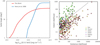 |
Fig. 2. Left: ROSAT NEP Raster Survey sensitivity function (red) compared with the RASS NEP survey of H06 (blue). Right: characterization of extended sources in the diagram of existence vs. extent likelihood. Red circles correspond to AGN1, blue circles to AGN2, pink circles to normal galaxies, green squares to clusters of galaxies, and yellow asterisks to stars. Black circles around the symbols indicate sources from the H06 catalogue. This figure, and the corresponding following figures, are only shown for the unique optical counterparts (see Sect. 4.4). Bright point sources (AGN, stars) appear to be extended because of the imperfect description of the PSF in the ML algorithm. The dashed line shows an empirical separation between true and spurious extension. |
3.4. Extended source analysis
The ML algorithm is very useful for the separation between point sources and clusters. It weights different photons according to the size of their individual PSF model, and therefore is arguably the most sensitive method for detecting extended sources in a photon-starved situation, where the extent is not much larger than the PSF. However, because of the necessary approximations in the description of the actual PSF, which depends on the off-axis angle and energy and also has extended scattering wings, the method tends to detect spurious extents in bright X-ray point sources. This is shown in Fig. 2 (right), where the extent likelihood is compared to the existence likelihood for the whole X-ray catalogue. Most clusters from the H06 catalogue are clearly segregated from the rest of the sample, with extent likelihoods Lext ≥ 4 − 5. However, above existence likelihoods of Lexi ≥ 50 the bright point sources (yellow stars and red AGN1 from H06) are creeping into the significantly extended area. We therefore empirically determined the dashed line to discriminate truly extended sources. There is one star from H06 (#3970), which appears significantly extended with an extent likelihood Lext = 12.4. There are actually two bright stars in the same error circle, so that the extent could be due to the double star nature. An additional complexity occurs in the case of AGN residing in clusters of galaxies, which may show X-ray extent despite being identified with a point source. The most interesting case is the AGN1 #5340 in the H06 catalogue, the object in the top right corner of Fig. 2 (right). This is the well-known bright HEAO-1 catalogue source H1821+643 (Pravdo & Marshall 1984) inside the massive cluster ClG 1821+64 (Schneider et al. 1992), later also detected by Planck through its Sunyaev-Zeldovich effect (Planck Collaboration XXIX 2014). An extended X-ray source superposed on the AGN point source extent has been independently measured for this object with the ROSAT HRI (Hall et al. 1997); therefore, the extent measured in our analysis is approximately correct and thus the dashed line maybe a bit too conservative.
4. Multi-band observations
4.1. HEROES optical/NIR wide-field imaging
The ultimate goal of HEROES (see e.g., Songaila et al. 2018) is to cover an area of 120 deg2 around the NEP, where the eROSITA X-ray all-sky survey (Merloni et al. 2012; Predehl et al. 2021) will have some of its deepest coverage. This survey utilizes the wide-field capability of the Hyper Suprime-Cam instrument (HSC; Miyazaki et al. 2012) on the Subaru 8.2 m telescope, as well as the MegaPrime/MegaCam and WIRCam instruments on the 3.6 m CFHT to map this large area. HEROES comprises grizy broad-band images with limiting magnitudes around 26.5−24.5 and NB816 & NB921 narrow-band images with limiting magnitudes around 24 from Subaru, as well as U- and J-band images with limiting magnitudes 25.5 and 22.1, respectively, from CFHT. So far an area of approximately 40 deg2 has been covered with HSC during 2016 July 1−10 and 2017 June 21−28 while the CFHT data were taken from 2016 March 18 to 2016 August 20. The HSC observations were acquired in a closely packed set of dithered observations described in detail in Songaila et al. (2018).
A formal publication of the HEROES catalogue is in preparation. Here we give some basic information about our data reduction process. Rather than using the HSC standard pipeline, which at the time of the massive data reduction task was not yet available to us, we analysed all HSC images with the Pan-STARRS Image Processing Pipeline (IPP; Magnier et al. 2020a), which was well tested and available on a dedicated computer cluster allowing fast processing of the large data volume. The IPP pipeline can be adapted to any wide-field imaging dataset, as long as the instrument calibration characteristics are incorporated. For HSC this required mainly the accurate description of the significant differential image distortion across the large FOV. The details of the Pan-STARRS Pixel Processing (i.e. the detrending, warping, and stacking of the images) are described in Waters et al. (2020). Each exposure is cleaned from instrumental effects, and photometry and astrometry are performed by comparing the objects detected on the individual images with the Pan-STARRS reference catalogue. This process also yields the individual image quality in terms of seeing and photometric transmission. The seeing was typically very good during the observations, with a median around 0.7″ and a large fraction of photometric transparency. For stacking the images into a common pixel grid we selected exposures with seeing better than 1.36″ and photometric zero points not fainter than 0.3 mag from the median. Co-adding the images to a certain degree also reduces non-astronomical artefacts like the reflection ‘ghosts’ from bright stars outside the FOV. Faint sources are detected by forced photometry running simultaneously across all filters (Magnier et al. 2020b). If a source is detected with more than 5σ in any particular band, photometry is forced on all other bands. This allows us to calculate photometric redshifts for a large fraction of all sources. Whenever available, we used Kron magnitudes for this purpose. For each band we also obtain a star–galaxy separation parameter. The original HSC catalogue of objects detected significantly in at least one band contains 23.9 million objects. However, caution is required to avoid false positive detections because a single artefact in any band will produce an entry in the catalogue. Therefore, we have selected objects detected in at least two bands for the photometric redshift determination described below.
The CFHT WIRCAM J-band data was reduced and stacked with a custom version of the AstrOmatic image analysis system (Bertin et al. 2012), in particular using the packages SCAMP, SWarp, MissFITS, and SExtractor (Bertin & Arnouts 1996). The CFHT MegaCam U-band data were reduced and stacked with the excellent MegaPipe imaging pipeline at the Canadian Astronomy Data Center (courtesy Stephen Gwyn). The astrometric calibration was done with Gaia, and the photometric calibration with a combination of SDSS data and a nightly zero-point calibration from MegaCam on photometric nights. This photometric calibration was bootstrapped to the few non-photometric nights so that the zero-point calibration is self-consistent to 0.015 mag. Again, we used the Kron magnitudes for the subsequent analysis.
An example of the excellent HEROES image quality, and also the various artefacts produced by bright objects in the field, is given in Fig. 3 showing the shell around the planetary nebula NGC 6543 (Cat’s Eye Nebula) that was ejected by its predecessor red giant star. The actual PN in the centre of the image is completely over-exposed. The high density of faint background objects shows the excellent sensitivity of the data. The NEP lies at relatively low Galactic latitudes, and therefore contains a rather large number of overexposed foreground stars showing up in this image (in cyan). In order to obtain reliable optical photometry for brighter objects, which are saturated in the HEROES HSC images, we also made use of the SDSS DR16 (Ahumada et al. 2020), the Pan-STARRS DR1 & DR2 (Chambers et al. 2016), and Gaia DR2 (Gaia Collaboration 2018) catalogues. We also cross-correlated our samples with the far-UV and near-UV photometry from the GALEX surveys (Martin et al. 2005).
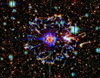 |
Fig. 3. False colour HEROES image of the shell around the planetary nebula NGC 6543 (Cat’s Eye Nebula) close to the NEP. Blue represents the HSC g-band image and predominantly shows the green [OIII] line. Green represents the HSC r-band and predominantly shows Hα. Red corresponds to the 4.5 μm Spitzer image and mainly shows dust emission. |
4.2. Mid-infrared observations of the HEROES field
For photometric information in the 3−25 μm band across the whole HEROES field we used the WISE all-sky survey catalogues. For the shorter wavelength W1 (3.4 μm) and W2 (4.6 μm) bands we used the CatWISE2020 all-sky catalogue (Eisenhardt et al. 2020) (see also Marocco et al., in prep.), containing about 1.89 billion objects observed by the Wide-field Infrared Survey Explorer (WISE and NEOWISE), both of which have higher sensitivity and higher angular resolution than the original ALLWISE catalogue (Cutri et al. 2013). The CatWISE2020 catalogue in the HEROES field contains 2.4 million objects and gives fluxes in the W1 and W2 band, which we converted to the AB magnitude system. For the longer wavelength W3 (12 μm) and W4 (22 μm) bands we used the original ALLWISE catalogue (Cutri et al. 2013), again converting to AB magnitudes. At the faintest magnitudes the CatWISE2020 and ALLWISE catalogues are, however, severely confusion limited. In the centre of the HEROES field, we therefore also made use of the Spitzer Observations of the Euclid Deep Field North (Moneti et al., in prep.).
The ESA Euclid mission is making great progress towards its launch, scheduled in 2022. Euclid’s main goal is to survey a large fraction of the sky and image billions of galaxies to investigate dark energy and dark matter over the history of the Universe. Roughly 10% of the observing time will be dedicated to the Euclid Deep Fields, repeatedly observing three specific areas of the sky, covering a total of 40 deg2. These three fields were carefully selected to contain a minimum of bright stars, and low dust emission and zodiacal light. In addition, these fields already have substantial multi-wavelength coverage, and will be observed with other space observatories, enabling us to perform a large amount of ancillary science. One of these fields encompasses an area of 10 deg2 around the NEP, in the middle of the HEROES field. The NASA Spitzer telescope has performed a large survey (P.I. P. Capak) of two Euclid Deep Fields, the Euclid/WFIRST Spitzer Legacy Survey (Capak et al. 2016). A total of 5286 h of Spitzer observing time are distributed over 20 deg2 split between the Chandra Deep Field South and the NEP, with an exposure time of 2 h per pixel. The primary goal is to enable definitive studies of reionization, z > 7 galaxy formation, and the first massive black holes. The data will also enhance the cosmological constraints provided by Euclid and Nancy Grace Roman Space Telescope (WFIRST). We are using a preliminary Spitzer data product. The final survey is being prepared for publication as part of the Spitzer Cosmic Dawn Survey (Moneti et al., in prep.), covering the three Euclid deep fields and several other Euclid calibration fields. These authors developed a new IRAC data processing pipeline and used the availability of highly precise astrometry available from Gaia to reprocess nearly all available Spitzer data in this field (excluding short observations like calibrations on bright stars), which will be essential for the Euclid calibration and for high-redshift legacy science. Figure 4 (left) shows the sky coverage of the two channels 3.6 μm (I1) and 4.5 μm (I2) with the widest deep coverage of the NEP. We used SExtractor (Bertin & Arnouts 1996) to extract source positions and magnitudes from the IRAC images in these two bands, yielding a catalogue of almost one million sources.
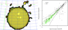 |
Fig. 4. Left: map of the Spitzer IRAC 3.6 μm (green) and 4.5 μm (red) coverage in the Spitzer Cosmic Dawn Survey around the NEP (Moneti et al., in prep.). Right: comparison between spectroscopic and photometric redshifts in our sample. Green circles are 541 ‘clean’ galaxies with spectroscopic redshifts in the HEROES field. Black dots are a sample of 263 AGN with spectroscopic redshifts in the field. The dashed and dotted lines refer to a redshift error of Δz/(1 + z) = ±0.15. |
4.3. Photometric redshifts
Based on the grizy HSC detections, we joined the GALEX, MegaCam, HSC, WIRCAM, SDSS, Pan-STARRS (partially), CatWISE2020, ALLWISE, and Spitzer IRAC catalogues into a single source list by association through positional matching. For the UV, optical, and NIR images and for the IRAC catalogue we allowed a maximum distance of 1″, while for GALEX and WISE we allowed a maximum of 3″. This way we obtained a combination of a maximum of 22 photometric bands (GALEX FUV & NUV, HEROES UgrizyJ plus NB816 & NB921, SDSS ugriz, as well as CatWISE2020 W1 & W2, ALLWISE W3 & W4, and IRAC I1 & I2 bands). Ideally, for the highest accuracy of photometric redshifts, the forced aperture photometry should be used in all bands. However, this is not possible in the case of a combination with catalogues from the literature. In some cases of very faint optical counterparts or objects confused with brighter nearby sources, we determined the correct magnitudes through manual aperture photometry.
A nice review of the application of photometric redshift techniques in modern wide-field surveys is given by Salvato et al. (2019). We determined photometric redshifts using the LePhare code (Arnouts et al. 1999; Ilbert et al. 2006). We followed the procedure described in Ilbert et al. (2009), basically fitting three different model families (galaxies, AGN, and stars) to the spectral energy distribution. For the galaxy SED templates we used the models from Laigle et al. (2016), including emission lines. For AGN we applied the specific modifications described in Salvato et al. (2009), wherever possible correcting for time variability between the SDSS and HEROES data, and taking the different SED templates used for point-like and extended AGN in Ananna et al. (2017). Because we include the WISE W3 & W4 mid-IR bands, we had to extrapolate some of the Ananna et al. (2017) hybrid galaxy and QSO SEDs to longer wavelengths. Our AGN photometry also required us to include the heavily absorbed TORUS model SED from Polletta et al. (2007). We adopted the Small Magellanic Cloud extinction law from Prevot et al. (1984) (see Salvato et al. 2009) to allow for intrinsic reddening of the sources, exploring E(B − V) values from 0 to 0.35 in steps of 0.05. Before the final fit we made slight adjustments to the zero points for each band, using the LePhare self-calibration procedure with 541 spectroscopic redshifts for clean galaxies (i.e. no AGN contribution, not confused, intermediate magnitudes) and 263 AGN with spectroscopic redshifts observed by HEROES in the field.
Figure 5 shows four high-quality examples of photometric redshift fits for X-ray detected AGN candidates, illustrating different spectral energy distributions. The MRK231 and TORUS SEDs have the largest relative mid-IR contributions, and sizeable number of X-ray counterparts (16 and 5, respectively), and even more mid-IR selected AGN (54 and 26, respectively) require these models. They are reminiscent of the Spitzer power law AGN SEDs detected in the Chandra deep fields (Donley et al. 2007). The TORUS SED model from Polletta et al. (2007) is an addition compared to the work of Salvato et al. (2009) and Ananna et al. (2017).
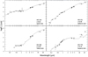 |
Fig. 5. Some high-quality examples of photometric redshift fits to X-ray counterparts, illustrating different AGN SED models. The MRK231 and TORUS spectra have the largest mid-IR fraction of all chosen models. |
We checked the quality of the photometric redshifts using the 541 reference galaxies (see the green circles in Fig. 4, right). The fraction of catastrophic outliers with |Δz|/(1 + z) ≥ 0.15 is only 4.6%, and the rms error of all galaxy photometric redshifts is ⟨|Δz|/(1 + z)⟩ = 0.033. The accuracy of the galaxy photometric redshifts is thus quite comparable to other surveys using broad-band photometry, but somewhat worse than e.g., those in the COSMOS field (Ilbert et al. 2009; Salvato et al. 2009; Laigle et al. 2016), mainly because COSMOS has a large number of intermediate band filters and much deeper imaging. We also compared the photometric and spectroscopic redshifts for the reference sample of 263 AGN in the field (black dots in Fig. 4, right panel). The fraction of catastrophic outliers is about 22%, and these are dominated by relatively bright AGN1. The rms error of all AGN photometric redshifts is ⟨|Δz|/(1 + z)⟩ = 0.06. In about 4% of all cases there is a secondary maximum in the photometric redshift probability distribution fitting better to the spectroscopic redshift. This quality is very similar to the results obtained by Ananna et al. (2017) for a sample of similar quality. Broad-band photometric redshifts for AGN1 are notoriously difficult for several reasons: their SEDs are practically power laws with superposed emission lines, which are not prominent in broad photometric bands. Time variability or photometric errors can cause spurious spectral features, which the SED fit clings to. However, despite the potentially erroneous photometric redshifts, the classification as AGN is unique. Therefore, our photometric redshifts are more than sufficient for a crude optical identification and source classification of the X-ray counterparts.
4.4. Optical identifications
The first step towards the optical identification of X-ray sources is the astrometric correction, which was already applied as part of the data preparation in Sect. 2. Therefore, the final output catalogue does not need further astrometric corrections. Optical identification is an iterative procedure, which in the case of relatively large error circles with multiple possible counterparts has a significant statistical uncertainty. The results therefore contain a probabilistic element, which is addressed below. The availability of the optical identification catalogue of H06, as well as the existence of a number of additional spectroscopic redshifts from the literature, are important prerequisites for the identification procedure. The NEP field is at a comparatively low Galactic latitude (b ≈ 28°), and therefore contains a large number of stars, many of which may also be faint X-ray sources. The optical position accuracy for bright stars is reduced, partially because they are often saturated in the deep CCD images. Wherever possible, therefore, we make use of the Gaia DR2 catalogue (Gaia Collaboration 2018).
Arguably the most important element of reliable identifications is the existence of the mid-IR catalogues from WISE and Spitzer. As we show below, the identification procedure for the 805 X-ray catalogue sources yields 766 high-likelihood optical candidates (identification quality IQ = 2), while in 39 cases there is an ambiguity with several possible counterparts (IQ = 1). There are 74 additional and possibly interesting objects in the error circles of high-likelihood counterparts, which are noted in the optical ID catalogue with IQ = 0. The following figures only show the 766 high-likelihood (IQ = 2) counterparts.
Figure 6 shows the offsets in right ascension and declination between the position of the X-ray source and that of the high-likelihood optical counterpart. Figure 7 (left) shows the cumulative distributions of position offsets (in arcseconds) for AGN (red); stars (yellow); and galaxies, clusters, and groups (green), identified below. AGN show the narrowest distribution, with a half-radius of 8.5″. Stars, on the other hand, have a somewhat wider distribution (half-radius 9.8″). This indicates that about 15% of the stellar identifications may be incorrectly associated, likely due to the large density of stars in the field. Clusters, groups, and individual galaxies have an even wider distribution. This may be due to the fact that the X-ray emission is not always centred on the brightest galaxy. We therefore use only AGN to calibrate the identification procedure. The first step is the determination of possible systematic position errors in the dataset. The ML X-ray detection algorithm gives the statistical position error (see Table 1), which can be compared to the distribution of counterpart offsets. For this purpose, we selected a reference sample of 231 high-quality AGN identifications, consisting of 141 AGN from H06, 10 other AGN with spectroscopic redshifts from the literature, and 80 high-quality AGN identifications selected from their mid-IR colours (with WISE W1 − W2 > 0.8; see Assef et al. 2013). First, we calculate the cumulative distribution of position offsets in units of the 1σ statistical position errors, which is shown as a grey line in Fig. 7 (right). This is significantly wider than the Gaussian model expectation, shown as black dashed curve. We then iteratively applied a systematic position error in quadrature to the statistical errors, until we found a reasonable match with the Gaussian expectation at a systematic error value of 3″. The corresponding cumulative distribution for our reference AGN sample is shown as the red curve. We then applied the same systematic error to the remaining 301 AGN identifications in the sample. Their cumulative position offsets are shown as the blue line in Fig. 7 (right). We also tested the normalized offset distributions separately for AGN1 and type 2 AGN (AGN2) for both the reference sample and the remaining AGN and did not find significant differences. The fact that all normalized offset distributions almost perfectly match the Gaussian expectation for the reference sample, which is typically from brighter X-ray objects, and for the fainter remaining AGN, confirms the accuracy of the ML errors as well as the systematic errors.
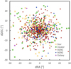 |
Fig. 6. Separation between X-ray and optical–NIR counterparts in arcseconds of right ascension and declination. The symbols are the same as in Fig. 2 (right). |
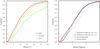 |
Fig. 7. Left: cumulative distribution of position offsets (in arcseconds) for different classes of sources. AGN have a narrow distribution with a half-radius of 8.5″, while stars have a slightly wider distribution (9.8″), indicating some possible misidentification among ∼15% of the stars. Clusters and groups have an even wider distribution because the X-ray emission is not always centred on the brightest galaxy. Right: cumulative distribution of position offsets in units of the 1σ position errors compared to a Gaussian model (black dashes). The grey line shows the distribution for 231 high-quality reference AGN (see text) before the application of a systematic position error. The red line shows the same 231 reference AGN after a systematic position error of 3″ has been applied to each statistical error. The blue line shows the offset distribution for the remaining 301 AGN applying the same 3″ systematic position error. |
We now can correlate the whole sample both with the optical (HEROES) and the mid-IR (WISE, Spitzer) catalogues to look at the number and magnitude distribution of the expected counterparts in the X-ray error circles, both the real counterparts and random field associations. We use a correlation radius of 2.5σ around each of the 805 X-ray sources to obtain the cumulative iAB and W1 magnitude distributions of objects, respectively, shown by the green lines in Fig. 8. The blue lines show the magnitude distribution of field objects within 805 randomly chosen circles of the same 2.5σ radius. The dashed red lines show the difference between X-ray error circles and field circles (i.e. the expected cumulative magnitude distribution for all counterparts associated with the X-ray sources). This gives the possibility of having more than one physical association per error circle (e.g., pairs, groups or clusters of galaxies, merging AGN, or star clusters). In making this subtraction one has to take care of the effect discussed in Brusa et al. (2007) and Naylor et al. (2013), namely that the magnitude distribution of field galaxies around bright objects is significantly shallower than around faint objects, leading to negative values in the subtraction. The dashed red lines have therefore been calculated piece-wise in different magnitude intervals before constructing the cumulative distribution. The solid red lines show the actual magnitude distribution of the selected best optical counterparts in Table 3. For magnitudes < 19 the dashed and solid red curves are quite close, indicating that the large majority of the selected best counterparts should be correct. At fainter magnitudes the dashed red curves increase above the solid red curves, up to values of 2.7 and 1.5 at iAB = 25 and W1 = 22, respectively. This is likely due to some true physical associations (e.g., interacting pairs of galaxies or clusters and group galaxies appearing in the same X-ray error circle).
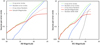 |
Fig. 8. Cumulative magnitude distributions in circles with 2.5σ error radii around the 805 X-ray sources (green line), and the same number of randomly chosen positions (blue line). The dashed red line shows the difference between source and random circles, while the thick red line shows the actual magnitude distribution of the X-ray counterparts. Left: Subaru HSC i band. Right: CatWISE2020 W1 band. The dotted black line shows the cumulative distribution of random mid-IR selected AGN candidates with W1 − W2 > 0.8. |
At magnitudes iAB and W1 > 19.5 the expected number of field objects per error circle increases above one, reaching values of ∼20 and ∼6 at iAB = 25 and W1 = 22, respectively. In this situation the optical identification purely by positional association becomes meaningless. We therefore have to introduce additional information and prior expectations into the identification process. As discussed above, this is naturally a probabilistic approach and no longer yields unique identifications. In principle there is the elaborate Bayesian multi-catalogue matching tool NWAY3 (Salvato et al. 2018), where several input catalogues can be cross-matched and a number of priors can be introduced, which also calculates the likelihood for every possible positional coincidence. However, in the case of incomplete catalogue information, and in the presence of significant systematic errors (e.g., non-astronomical false positive detections in the optical catalogue) or the presence of source confusion both in the X-ray catalogue and in the CatWISE2020 catalogue it is very cumbersome to construct the appropriate prior for this method.
Figure 9 gives a visual impression of the difficulty of optical identification in the complicated situation of faint optical counterparts with relatively large error circles and possibly confused settings. ROSAT X-ray contours are superimposed in a logarithmic scale on a false-colour image with the Spitzer bands I2 (red) and I1 (green) and the HEROES i-band image (blue). This 18′×15′ image is centred on the planetary nebula NGC 6543 close to the centre of the HEROES field (see also Fig. 3). The ML X-ray positions are shown as cyan circles with 2σ error radii, and the final optical counterparts are indicated with magnitudes in magenta. The planetary nebula (XID #389) is clearly detected in X-rays, but there is another X-ray source (XID #377) close to and confused with it. This source has two possible stellar counterparts, but the XMM-Newton image clearly selects the brighter star. The faint X-ray source (XID #388) in the lower centre of the image has two credible AGN counterparts. Given these difficulties, we had to resort to the tedious task of visually inspecting every individual error circle and manually selecting and characterizing the most likely optical counterpart, considering a number of prior expectations. Previously published deep X-ray surveys (e.g., Brandt & Hasinger 2005) show that the largest fraction of X-ray sources at our flux limit are AGN, followed by stars, and clusters of galaxies. This is also the case for the H06 catalogue. Stars can usually be discriminated rather easily; at the same X-ray flux they are about 5 mag brighter than both AGN and cluster galaxies (see e.g., Fig. 10). However, given the rather large density of stars in our field, there is the possibility for misidentification. Brighter and lower-redshift clusters of galaxies can often be readily identified through their extended X-ray emission or the concentration of bright galaxies associated with the X-ray source. However, there are also fainter and higher-redshift cluster candidates without significant X-ray extent. For the objects with unclear identifications we first searched for a possible cluster or group by looking for photometric redshift concentrations in a circle with radius of 30−120″ around the X-ray source, and indeed could identify a number of photometric cluster candidates this way. Higher-redshift (z > 0.8) clusters, where the optical magnitudes of even the brighter cluster members are very faint and thus do not stand out against the field galaxies, are easier to identify in the mid-IR images.
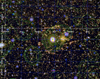 |
Fig. 9. Cutout (18′×15′) of the centre of the HEROES field. ROSAT X-ray contours (green) are superposed on a false-colour optical–mid-IR image with the HSC i band in blue and the Spitzer I1 and I2 bands in green and red, respectively. ML X-ray error circles are shown in cyan with the radius of 2σ. Optical counterpart magnitudes are indicated in magenta. |
Active galactic nuclei with optical counterpart magnitudes iAB < 19 − 20 are typically the brightest and often point-like objects in their X-ray error circle, and thus easy to identify. Problems arise, when the optical counterparts are fainter than iAB > 20. Then the likelihood to have an un-associated field object with a magnitude brighter than the actual X-ray counterpart in the error circle increases substantially. Also, at fainter X-ray fluxes and optical magnitudes the fraction of unobscured AGN1 decreases, and absorbed or obscured AGN2, which are harder to discriminate from normal galaxies, become more abundant. In this situation mid-IR imaging becomes crucial. In general, both AGN1 and AGN2 are brighter in the mid-IR channels than normal galaxies, and very often the X-ray counterpart is the brightest WISE or Spitzer source in the error circle. Most AGN can be readily identified through their peculiar mid-IR colours (see e.g., Stern et al. 2012; Assef et al. 2013). We used the classical criterion W1 − W2 > 0.8 to identify mid-IR AGN candidates. The dotted black line in Fig. 8 (right) shows the randomly expected number of mid-IR selected AGN per X-ray error circle, which is below 1 for the relevant magnitude range, thus confirming the reliability of this selection. Assef et al. (2013) show that this selection contains some interlopers from normal galaxies with redshifts z > 1.5, which could in principle be discriminated using the Spitzer [5.8]−[8.0] colours. Since we do not have longer wavelength Spitzer photometry of the HEROES field and the WISE W3 & W4 bands get confusion limited at faint magnitudes, we resorted to looking at the spectral energy distribution of the photometric redshift fits and gave priority to candidates containing a significant AGN contribution in their model SED. Finally, at faint magnitudes (e.g., W1 > 20) even the mid-IR colour selection runs into problems, first because the statistical errors in the detection hamper the proper colour determination, and secondly, because the WISE data become significantly confusion limited. For the central 10 deg2 of our survey covered by Spitzer we could, however, go a step further because these images resolve the WISE source confusion and also go about a magnitude deeper. In a handful of cases we even found Spitzer sources in the centre of otherwise empty X-ray error circles, which we termed as ‘infrared dropouts’. We manually determined limiting optical magnitudes and detections at the corresponding positions and could determine photometric redshifts in the range 1 < z < 6 for these objects.
For each of the potential X-ray counterparts we determined photometric redshifts as described in Sect. 4.3. We visually inspected each photometric redshift fit and manually clipped outliers. For missing bands, we manually determined the magnitude values or upper limits. For AGN, in addition to the photometric redshift, we also determined a coarse characterization based on the best-fit model SED. Models with a clear type 1 broad line contribution to the SED (> 10% in case of hybrid galaxy or AGN models) with intrinsic extinction E(B − V) < 0.2 were characterized as AGN1, SED models with type 2 character (Seyfert-2, QSO-2, star forming galaxies) and/or intrinsic extinction E(B − V)≥0.2 were characterized as AGN2. Pure galaxy SED models with intrinsic extinction E(B − V) < 0.2 were characterized as galaxies if the corresponding X-ray luminosity was below log(LX/(erg s−1)) < 42, and as AGN1 for higher luminosities. It is clear that this characterization is only indicative and does not replace a true spectroscopic identification for individual objects. However, sample properties of object classes can still be assessed.
In finally assessing an identification quality (IQ) for each possible counterpart, we also took into account the position information for 477 X-ray sources from the literature (431 matches with 2RXS, 83 with 4XMM-DR9, and 40 with XMMSL2; see Sect. 4.5 above). The 2RXS catalogue gave better identification accuracy for 7 of the 431 common objects (1.6%), while XMM-Newton gave unique new positions for 10 out of 123 common sources (8.1%). Overall, our identification quality can therefore be regarded as quite reliable. An identification quality of IQ = 2 means a high-likelihood single optical counterpart. There are 766 X-ray sources in this category. An identification quality of IQ = 0 means a rejection of this counterpart in the presence of a better counterpart; 74 sources are in this category, i.e. about 10% of the IQ = 2 counterparts contain one or more less likely candidates, mainly unrelated galaxies or stars. An identification quality of IQ = 1 means there are several possible counterparts without a clear priority ranking. There are 39 X-ray sources in this category (i.e. ∼5% of the sample), with a total of 80 possible counterparts that are dominated by AGN candidates. In this category there are also a number of possible dual AGN with two AGN candidates at similar redshift within the X-ray error circle. Table 2 gives a summary of classifications in the three quality classes. We compare this with the equivalent samples of soft X-ray selected objects in the COSMOS field. Table 3 gives the catalogue of all possible optical counterparts for the X-ray sources, including their identification quality.
Summary of optical identifications.
4.5. The ROSAT NEP Optical Identifications Catalogue
Table 3 gives the final catalogue of optical identifications for the 805 X-ray sources in Table 1, again in abbreviated form. The complete catalogue is available at the CDS. For convenience we number the columns consecutively carrying on from Table 1. Most of the bright star magnitudes are from the Gaia DR2 catalogue (Gaia Collaboration 2018), while most of the galaxy magnitudes are from the Subaru HSC i band (or z band), but there are small additions from Pan-STARRS and SDSS. Most spectroscopic redshifts are from the literature, the majority from H06, but others are from the NASA Extragalactic Database (NED). For a small number of objects specific spectroscopic observing runs have been performed with the Keck DEIMOS and KCWI instruments, and with HYDRA on the WYIN telescope; details of these runs will be published elsewhere. The photometric redshifts are from the LePhare analysis described above. Column (21) gives the logarithm of the observed 0.5−2 keV luminosity (i.e. no rest-frame correction). Column (22) gives a comment for most sources. Objects from H06 are identified by their catalogue numbers in the comment column.
ROSAT NEP Raster Candidate Optical ID Catalogue.
4.6. Multi-wavelength properties of X-ray counterparts
Figures 10–14 display the results of the optical identification process for the NEP raster scan catalogue. Figure 10 gives the classical correlation diagram between X-ray flux and optical magnitude (left) and W1 magnitude (right). This diagnostic diagram was originally introduced by Maccacaro et al. (1988) for the Einstein Medium Sensitivity Survey, and was later applied to numerous occasions, for example the HELLAS2XMM Survey (Fiore et al. 2003) and the XMM-Newton survey of the COSMOS field (Brusa et al. 2010). The different source classes segregate in a well-known fashion in this diagram, with AGN1 following a relatively tight correlation around a constant X-ray–to–optical flux ratio, which is calculated as fXO = log(FX/Fopt) = log(FX) + 0.4⋅iAB + 5.37. The dashed line in the left figure indicates an X-ray–to–optical flux ratio of unity, i.e. fXO = 0, while in the right diagram it gives the empirical discrimination line between AGN and stars and galaxies derived by Salvato et al. (2018). Clusters appear on average optically somewhat brighter, while stars are at significantly brighter magnitudes for the same X-ray flux. AGN2 are relatively rare at brighter X-ray fluxes, but their fraction increases towards lower fluxes. There is a significant new class of optically very faint AGN at lower X-ray fluxes, with magnitudes iAB > 22 and X-ray to optical flux ratios fXO = 1−3. These are also dominant in the population of infrared dropouts with i–IR > 3 discussed below. Their photometric fits indicate spectral energy distributions with significant AGN contributions in the redshift range 1 < z < 6. There are 11 AGN1 in this category (about 3% of the AGN1 sample); a total of 24 AGN2 also fall in this group, which is almost 1/3 of the AGN2 population in our sample. In the right-hand diagram, when plotted against mid-IR magnitudes, these objects are less apparent, but still among those with the faintest mid-IR magnitudes. Open triangles show the sample of mid-IR selected AGN candidates (see below) at their 2σ X-ray flux upper limits. A large number of these also fall in the category of optically very faint infrared dropouts.
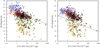 |
Fig. 10. Left: AB magnitude vs. X-ray flux. The symbols are the same as in Fig. 2 (right); also shown are the X-ray upper limit fluxes for a sample of AGN candidates selected from mid-IR colours (red triangles for AGN1 candidates and blue triangles for AGN2 candidates). The dashed line indicates an X-ray–to–optical flux ratio of fXO = 1. Right: as in the left figure, but with the CatWISE2020 W1 magnitude on the x-axis. Here the dashed line shows the empirical discrimination between AGN and other objects defined in Salvato et al. (2018). |
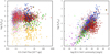 |
Fig. 11. Left: X-ray–to–optical flux ratio fXO vs. X-ray flux. Shown are the ROSAT NEP raster scan catalogue objects (colours as in Fig. 6 without the H06 objects indicated); at fainter fluxes the objects from the largely spectroscopically identified Chandra legacy survey of the COSMOS field (Marchesi et al. 2016) are also shown (small open symbols and the same colours). The large orange diamond gives the position of the highest-redshift radio loud quasar CFHQS J142952+544717 recently identified in the eROSITA all-sky survey (Medvedev et al. 2020). Right: X-ray–to–optical flux ratio vs. X-ray luminosity. Same symbols as the left figure, but the upper limits from the mid-IR AGN candidates are added as red and blue triangles. The dotted line refers to the highest-luminosity object XID803, which has a second photometric redshift solution at lower luminosity. |
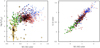 |
Fig. 12. Left: X-ray to optical flux ratio fXO vs. CatWISE2020 W1 − W2 mid-IR colours. Right: Spitzer IRAC I1 − I2 vs. CatWISE2020 W1 − W2 mid-IR colour. Symbols are the same as in Figs. 10 and 11. |
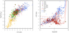 |
Fig. 13. Left: X-ray–to–optical flux ratio fXO vs. the optical to infrared colour i–IR (symbols are the same as in Fig. 6, but with the addition of the of mid-IR selected AGN candidates as in Fig. 10). Right: optical to infrared colour i–IR as a function of redshift for AGN1 (red), AGN2 (blue), and galaxies (magenta). SED models for QSO1, QSO2, Sy1, and Sy2 from the photometric redshift fits are overplotted (see legend). |
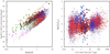 |
Fig. 14. Left: 0.5−2 keV X-ray luminosity vs. redshift for the ROSAT NEP and Chandra COSMOS data (same symbols as in Fig. 11). Right: X-ray to optical flux ratio fXO vs. X-ray flux for all AGN from the Chandra COSMOS sources (small open circles), the mid-IR sample upper limits (triangles), the ROSAT NEP raster scan (solid circles), the SPIDERS 2RXS catalogue (open squares), and the SPIDERS XMMSL2 sources (plus signs). AGN1 are shown in red, AGN2 in blue symbols. CFHQS J142952+544717 is shown as orange diamond. |
Figure 11 (left) shows the NEP sources with the X-ray–to–optical flux ratio fXO on the y-axis. In addition, we plot the optical identifications from the Chandra legacy survey of the COSMOS field (Civano et al. 2016; Marchesi et al. 2016; Hasinger et al. 2018; Gozaliasl et al. 2019) using the same colours but smaller open symbols. Despite the difference in X-ray flux limit of about a factor of 10, the X-ray–to–optical flux ratio distributions of the two samples are very similar, and overlap at the bright end. The fraction of stars is significantly smaller in COSMOS than in the NEP field. This is due to the lower Galactic latitude of the NEP (δ ∼ 30°) compared to the COSMOS field (δ ∼ 42°), but also due to the reduction of stars at fainter X-ray fluxes. The large orange diamond shows the position of the highest-redshift radio loud quasar CFHQS J142952+544717, the most X-ray luminous quasar ever observed at z > 6, which was recently identified in the eROSITA all-sky survey (Medvedev et al. 2020). Figure 11 (right) shows the same objects as in the left figure, but now with the (observed) 0.5−2 keV X-ray luminosity on the x-axis. In addition, the X-ray upper limits are plotted as open triangles, as in Fig. 10. There is a general correlation between X-ray luminosity and X-ray–to–optical flux ratio, at least for galaxies, clusters and AGN2. This is likely caused by the optical counterparts with galaxy-type SEDs getting redder and thus relatively fainter with redshift. The more luminous AGN1, however, for which the SED is dominated by a power law spectrum, retain their X-ray–to–optical flux ratios in the range −1 < fXO < 0.5 even at higher redshifts. There is one AGN1 at z = 4.43 with an X-ray luminosity log(LX/(erg s−1)) = 46.8 erg s−1, even higher than that of CFHQS J142952+544717. However, the photometric redshift probability distribution for this object shows a second peak at lower redshifts (z ∼ 0.56), which would bring the luminosity down to more ballpark values, indicated by the dotted line. The true redshift needs to be confirmed spectroscopically.
Figures 12 and 13 show the power of mid-IR colours for the X-ray source characterization and AGN selection. Figure 12 (left) displays the X-ray–to–optical flux ratio as a function of the CatWISE2020 W1 − W2 colour. AGN dominate at W1 − W2 > 0.7, but are also present down to W1 − W2 > 0.3. The classical mid-IR AGN selection of Stern et al. (2012) assumes W1 − W2 > 0.8. Clusters and AGN have overlapping ranges of fXO, but clearly segregate in the mid-IR colours. There is a number of bright stars with relatively large W1 − W2 colours, which are likely spurious due to saturation in the WISE images. This figure also contains the even redder selection of mid-IR AGN candidates without X-ray detections (triangles, see below). Figure 12 (right) shows the comparison between the mid-IR colours from CatWISE2020 (W1 − W2) and the I1 − I2 colours from the Spitzer IRAC catalogue in the overlapping region. There is a clear correlation between the two mid-IR colours, but in particular for the faintest mid-IR objects the identification quality is significantly improved in the Spitzer data. Figure 13 (left) shows the correlation between the X-ray–to–optical flux ratio fXO and the optical to infrared colour i–IR. Here the infrared magnitude IR is either taken as the CatWISE2020 W1 or the Spitzer IRAC I1 value. While the AGN1 form a rather compact clump centred around fXO = −0.5 ± 1 and i–IR = 1.5 ± 1 in this diagram, the AGN2 are drawn out over a larger range of values up to fXO < 3 and i–IR < 8. We define infrared dropouts as objects with i–IR > 3. Figure 13 (right) shows the run of the optical to infrared colours with redshift in comparison to some representative SED models. There is a clear segregation between AGN1, which maintain rather blue colour throughout all redshift ranges up to z < 5, and AGN2, which turn into infrared dropouts above redshifts z > 1. The most luminous QSO1 and QSO2 templates straddle the range of optical to infrared colours, while the lower luminosity Seyfert1 and Seyfert2 models lie in between. The mid-IR selected AGN candidates with X-ray upper limits (triangles, see below) follow the same trends. Interestingly, the highest-redshift radio loud quasar CFHQS J142952+544717 from the eROSITA All-sky survey (Medvedev et al. 2020) perfectly fits the QSO1 template for its redshift of z = 6.18. Finally, Fig. 14 shows the coverage of the different samples in the X-ray luminosity versus redshift plane. The ROSAT NEP data reaches significantly higher X-ray luminosities of log(LX/(erg s−1)) < 46) than either the COSMOS sample or the list of mid-IR selected upper limits. This is only topped by the highest X-ray luminosity source CFHQS J142952+544717 discovered in the eROSITA all-sky survey (Medvedev et al. 2020) and possibly one of the AGN1 in our sample (see above). The upper redshift cut-off of all samples is similar, with the bulk of objects at z < 4 and a significant number of AGN1 and AGN2 candidates at z = 4−7.
4.7. X-ray properties of mid-infrared selected AGN
The richness and coverage of the HEROES NEP dataset allows for the selection of a high-quality AGN sample based purely on mid-IR colours. For this purpose, we use the overlapping range of the WISE and Spitzer coverage in the field and select objects with red W1 − W2 as well as I1 − I2 colours. Following the correlation between these two infrared colours shown in Fig. 12 (right), we chose objects with W1 − W2 > 1, I1 − I2 > 1 and the error δ(I1 − I2) < 0.2. A total of 185 mid-IR AGN candidates were selected this way. We applied the same photometric redshift determination and classification procedure as for the X-ray selected AGN above, yielding 88 AGN1 and 97 AGN2 candidates with median redshifts of approximately ⟨zAGN1⟩ = 1.5 and ⟨zAGN2⟩ = 2.3, respectively. We then offered the mid-IR AGN candidate positions to the ROSAT ML detection algorithm to determine X-ray count rates or upper limits for these objects at their fixed positions. We chose 95.4% upper limit count rates, corresponding to a Gaussian 2σ probability. Nine of the 186 mid-IR AGN candidates have significant X-ray detections (with Lexi > 12). Four of them are part of the X-ray catalogue in Table 1. The other five have not been detected, mainly because of confusion issues. X-ray fluxes and upper limits were determined in the same way as the X-ray sources above. The relevant data is shown as triangles in Figs. 10–14. In general, these correlations show that the mid-IR selected AGN candidates are a continuation in parameter space of the X-ray selected AGN. They have similar X-ray–to–optical flux ratios and similar optical to infrared colours to the X-ray selected population, but are typically a factor of a few fainter than the X-ray sources. Their photometric redshift fits are much more dominated by large mid-IR fraction SEDs (e.g., MRK231 and TORUS, see Sect. 4.3).
It is interesting to note that the median redshift of the mid-IR selected AGN2 is significantly higher than that of the AGN1 (see also Fig. 15). This is likely due to a selection effect in the mid-IR discussed by Assef et al. (2013). The mid-IR (W1 − W2) colour of AGN1 is reddest in the redshift range 1 < z < 2, and gets progressively bluer at redshifts z > 2 (see Fig. 1 of their paper). At redshifts z > 3, AGN1 completely fall out of the W1 − W2 > 0.8 criterion. A similar effect can be seen in Fig. 13 (right). This effect causes the mid-IR selection to systematically miss higher-redshift AGN1.
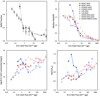 |
Fig. 15. Ensemble properties of AGN1 (red) and AGN2 (blue) grouped by X-ray flux. Filled symbols show the ROSAT NEP sample, open symbols the soft-band detected Chandra COSMOS sample. The triangles show the upper limits for the mid-IR selected AGN sample. Upper left panel: median redshifts. Upper right panel: median X-ray luminosities, and lower left: median X-ray–to–optical flux ratios. Finally, the lower right panel shows the AGN2 fraction (AGN/(AGN1 + AGN2) as a function of soft X-ray flux. |
We predict that most of the mid-IR selected AGN will be detected in the future deeper and harder eROSITA coverage of the NEP. Table 4 gives the catalogue of 185 mid-IR colour selected AGN candidates, again in abbreviated form. The complete catalogue is available at the CDS.
AGN candidates selected by mid-IR colours.
5. Discussion and conclusions
We compare the ensemble properties of our AGN with other soft X-ray selected samples over a wide range of limiting fluxes. In addition to the Chandra catalogue in the COSMOS field already displayed above, we include the second ROSAT all-sky source catalogue 2RXS (Boller et al. 2016), and the Second XMM-Newton Slew Survey Catalogue XMMSL2. The SPectroscopic IDentification of ERosita Sources (SPIDERS) survey, an SDSS-IV programme aimed at obtaining spectroscopic classification and redshift measurements for complete samples of sufficiently bright X-ray sources (Dwelly et al. 2017; Salvato et al. 2018; Comparat et al. 2020), is to date the largest systematic spectroscopic observation of X-ray selected samples. It targeted the 2XRS and XMMSL2 sources in a sky area of 5129 deg2 covered in SDSS-IV by the eBOSS survey. We used the Value Added Catalogs from the MPE SPIDERS home page4, which include cross-correlations with various galaxy cluster catalogues. The complete catalogues contain a total of 19821 and 2342 X-ray sources for 2RXS and XMMSL2, respectively. From the 2RXS SPIDERS catalogue we selected 10113 sources with detection likelihood Lexi > 10 in the total (0.1−2.4 keV) ROSAT band, and converted the X-ray fluxes to the 0.5−2 keV band assuming an unabsorbed power law spectrum with photon slope −2. For XMMSL2 we selected 1860 sources with a detection likelihood Lexi > 10 in the 0.5−2 keV band and used the corresponding soft fluxes given in the catalogue. We correlated the source lists with the SIMBAD and NED databases in order to obtain additional identifications beyond the original SPIDERS spectroscopic target selection. After this procedure, a total of 2607 and 227 objects remain unidentified in the 2RXS and XMMSL2 catalogues, respectively, corresponding to 26% and 12% incompleteness for the two selected subsamples. This allows a reasonably reliable assessment of ensemble properties of the different source classes, although the incompleteness can introduce some systematic errors in the analysis (see below). Following Comparat et al. (2020) we classified as unobscured AGN1 those catalogue entries with spectroscopic classes BALQSO, BLAGN, BLAZAR, QSO, QSO_BAL, as well as sources from the literature with a QSO or Seyfert 1 designation (Sy1, Sy1.2). We classified as AGN2 the all sources with spectroscopic class NLAGN, all sources classified as GALAXY that do not belong to a cluster of galaxies and have an X-ray luminosity log(LX/(erg s−1)) > 42, and sources from the literature with a Seyfert 2 designation (Sy1.5, Sy1.9, Sy2). This way we classified a total of 5541 and 1046 objects as AGN1 and 603 and 101 as AGN2 for the 2RXS and XMMSL2 catalogues, respectively. The X-ray–to–optical flux ratio as a function of X-ray flux for these sources is compared to the ROSAT NEP and COSMOS samples in Fig. 14 (right).
Figure 15 shows ensemble properties of the AGN1 and AGN2 samples grouped by 0.5−2 keV X-ray flux. The upper left graph clearly shows a strong increase in the fraction of AGN2 with decreasing X-ray flux. The mid-IR selected, non-X-ray detected AGN, assuming that their ensemble X-ray flux is somewhat below their median upper limit (3 × 10⁻¹⁵ erg cm−2 s−1), show an even larger AGN2 fraction. This is likely due to the selection effect discussed in Sect. 4.7. A dependence of the obscured AGN fraction on luminosity and redshift was first discussed by Lawrence (1991). A similar trend of increasing obscuration with decreasing X-ray luminosity has been observed in hard X-ray selected samples of AGN over a very broad range of fluxes, including the Chandra deep fields (Barger et al. 2005; Hasinger 2008).
However, looking at the median redshift (upper right), X-ray luminosity (lower left), and X-ray–to–optical flux ratio (lower right) ensemble properties, there is a significant difference between the ROSAT NEP and the other samples. In general, for AGN1 of all samples the median redshift increases; the median luminosity and the median X-ray–to–optical flux ratio decrease with decreasing flux across the whole range. In the overlapping flux ranges there are systematic differences between the samples, which could easily be explained by the systematics of source identification and characterization procedures (e.g., the identification or classification incompleteness or the difference between photometric and spectroscopic classification), but they are relatively small compared to the overall trends. The XMMSL2, 2RXS, and COSMOS AGN2 roughly follow the same trends in ensemble properties as the AGN1.
However, the ROSAT NEP AGN2 behave differently; at the faintest fluxes they have the highest median fXO of all samples. This is independent from photometric redshift errors, which could in principle introduce systematic effects, when comparing median luminosities. As discussed above, photometric redshifts of AGN2 have smaller uncertainties than those of AGN1. We can therefore conclude that the X-ray faintest ROSAT NEP AGN2 have somewhat larger redshifts and higher X-ray luminosities than the AGN1 at corresponding fluxes. The mid-IR selected AGN2 follow or even accentuate this trend.
As already demonstrated in Figs. 10–14, we see the emergence of a new population of high-luminosity, high-redshift obscured AGN2 that have not been recognized in previous X-ray selected AGN samples. The main new observational phenomenon is the comparatively high X-ray–to–optical flux ratio fXO of this AGN2 population, accompanied by a large fraction of infrared dropouts (see e.g., Fig. 13 left).
We have investigated why this population has not been recognized in previous X-ray surveys, in particular in the Chandra COSMOS-Legacy survey. The soft X-ray selected sample of this survey contains 2969 objects (Civano et al. 2016) and their original optical to IR identification catalogue (Marchesi et al. 2016) contains 74 objects with ambiguous, sub-threshold, or completely missing identifications. We looked at all these sources using the most recent publicly available deep optical (Subaru Hyper-Suprime-CAM), NIR (ULTRAVISTA), and Spitzer (SPLASH) image cutouts5 and found that 28 of these sources (38%) are indeed infrared dropouts according to our criterion (i–IR > 3), and thus correspond to the newly identified AGN2 population6. These objects have been included in the diagrams in Figs. 11 and 14, but their contribution to the overall sample of AGN2 in the COSMOS survey is relatively small, so that they do not appear as a dominant new population.
Similarly, the SPIDERS 2RXS and XMMSL2 catalogues contain a number of high fXO sources, but they are not dominant (see also Salvato et al. 2018). Due to the combination of larger solid angle, and sufficient X-ray sensitivity, together with the excellent HEROES multi-wavelength coverage and in particular the Spitzer mid-IR angular resolution and sensitivity, the ROSAT NEP sample reaches a dominant AGN2 population with optically very faint infrared X-ray counterparts (infrared dropouts), which turn out to be predominantly higher luminosity (log(LX/(erg s−1)) > 44), higher redshift (z > 1.5) AGN2. Their photometric redshift fits often require mid-IR dominated SEDs (e.g., MRK231 and TORUS models) reminiscent of the Spitzer power law AGN detected in the Chandra deep fields (Donley et al. 2007), albeit at higher redshifts. The same is true for the sample of mid-IR selected, but not X-ray detected AGN candidates.
Here it is worth noting that the Spitzer data are crucial in our analysis. At the faintest infrared magnitudes, where many of our X-ray counterparts reside, the WISE data is significantly confusion limited, which can easily produce spurious red IR colours, and also does not allow us to uniquely identify the often very faint optical counterpart. Only the higher angular resolution of the Spitzer data allows us to obtain secure IR colours and optical identifications at the faintest IR magnitudes.
Figures 11 (right) and 14 show that due to the combination of larger solid angle and sufficient sensitivity the ROSAT NEP sample reaches X-ray luminosities around log(LX/(erg s−1)) < 46 for all AGN, which is higher than previous X-ray survey values, which are typically limited at log(LX/(erg s−1)) < 45. The discovery of the highest X-ray luminosity quasar to date in the eROSITA all-sky survey (Medvedev et al. 2020) confirms this trend.
Our unique HEROES multi-wavelength dataset is important as a reference sample for future deep surveys in the NEP region, in particular for eROSITA, but also for Euclid and SPHEREX. We predict that most of the absorbed distant AGN should be readily picked up by eROSITA, but they require sensitive mid-IR imaging to be recognized as X-ray counterparts.
Hawaii eROSITA Ecliptic Pole Survey.
The remaining unidentified sources are typically objects blinded by bright nearby stars or galaxies.
Acknowledgments
We would like to thank an anonymous referee for very helpful suggestions to improve the manuscript. GH would like to thank Olivier Ilbert and Mara Salvato for important help with the LePhare photometric redshift code, and Mara as well for very helpful comments on the paper draft. We would like to thank Len Cowie for designing the HEROES survey, and the former IfA REU students Cameron White & Victoria Jones who have accompanied the HEROES observations and analysis, as well as taken a few HYDRA spectra of X-ray sources at the WIYN telescope. E.M.H. would like to acknowledge the NSF grant AST-1716093, partly funding the HEROES activities. We would like to acknowledge the excellent ROSAT data archive provided by the Max-Planck-Institute for Extraterrestrial Physics, Garching, Germany. This research has made use of data obtained from XMMSL2, the Second XMM-Newton Slew Survey Catalogue, produced by members of the XMM SOC, the EPIC consortium, and using work carried out in the context of the EXTraS project (“Exploring the X-ray Transient and variable Sky”, funded from the EU’s Seventh Framework Programme under grant agreement no. 607452). This research has made use of data obtained from the 4XMM XMM-Newton serendipitous source catalogue compiled by the 10 institutes of the XMM-Newton Survey Science Centre selected by ESA. This work is based in part on observations made with the Spitzer Space Telescope, which was operated by the Jet Propulsion Laboratory, California Institute of Technology under a contract with NASA and it also makes use of data products from the Wide-field Infrared Survey Explorer, which is a joint project of the University of California, Los Angeles, and the Jet Propulsion Laboratory/California Institute of Technology, funded by NASA. It is also based in part on data collected at Subaru Telescope, which is operated by the National Astronomical Observatory of Japan, as well as on observations obtained with MegaPrime/MegaCam, a joint project of CFHT and CEA/DAPNIA, at the Canada-France-Hawaii Telescope (CFHT) which is operated by the National Research Council (NRC) of Canada, the Institut National des Science de l’Univers of the Centre National de la Recherche Scientifique (CNRS) of France, and the University of Hawaii. The authors wish to recognize and acknowledge the very significant cultural role and reverence that the summit of Maunakea has always had within the indigenous Hawaiian community. We are most fortunate to have the opportunity to conduct observations from this mountain.
References
- Ahumada, R., Prieto, C. A., Almeida, A., et al. 2020, ApJS, 249, 3 [Google Scholar]
- Ananna, T. T., Salvato, M., LaMassa, S., et al. 2017, ApJ, 850, 66 [Google Scholar]
- Arnouts, S., Cristiani, S., Moscardini, L., et al. 1999, MNRAS, 310, 540 [NASA ADS] [CrossRef] [Google Scholar]
- Assef, R. J., Stern, D., Kochanek, C. S., et al. 2013, ApJ, 772, 26 [Google Scholar]
- Barger, A. J., Cowie, L. L., Mushotzky, R. F., et al. 2005, AJ, 129, 578 [NASA ADS] [CrossRef] [Google Scholar]
- Bertin, E., & Arnouts, S. 1996, A&AS, 117, 393 [NASA ADS] [CrossRef] [EDP Sciences] [Google Scholar]
- Bertin, E., Delorme, P., & Bouy, H. 2012, Astrophys. Space Sci. Proc., 29, 71 [NASA ADS] [CrossRef] [Google Scholar]
- Boese, F. G. 2000, A&AS, 141, 507 [NASA ADS] [CrossRef] [EDP Sciences] [Google Scholar]
- Boese, F. G., & Doebereiner, S. 2001, A&A, 370, 649 [NASA ADS] [CrossRef] [EDP Sciences] [Google Scholar]
- Boller, T., Freyberg, M. J., Trümper, J., et al. 2016, A&A, 588, A103 [NASA ADS] [CrossRef] [EDP Sciences] [Google Scholar]
- Bower, R. G., Hasinger, G., Castander, F. J., et al. 1996, MNRAS, 281, 59 [NASA ADS] [CrossRef] [Google Scholar]
- Brandt, W. N., & Hasinger, G. 2005, ARA&A, 43, 827 [Google Scholar]
- Brusa, M., Zamorani, G., Comastri, A., et al. 2007, ApJS, 172, 353 [NASA ADS] [CrossRef] [Google Scholar]
- Brusa, M., Civano, F., Comastri, A., et al. 2010, ApJ, 716, 348 [NASA ADS] [CrossRef] [Google Scholar]
- Capak, P., Arendt, R., Arnouts, S., et al. 2016, The Euclid/WFIRST Spitzer Legacy Survey, Spitzer Proposal [Google Scholar]
- Cappelluti, N., Brusa, M., Hasinger, G., et al. 2009, A&A, 497, 635 [NASA ADS] [CrossRef] [EDP Sciences] [Google Scholar]
- Chambers, K. C., Magnier, E. A., Metcalfe, N., et al. 2016, ArXiv e-prints [arXiv:1612.05560] [Google Scholar]
- Civano, F., Marchesi, S., Comastri, A., et al. 2016, ApJ, 819, 62 [Google Scholar]
- Comparat, J., Merloni, A., Dwelly, T., et al. 2020, A&A, 636, A97 [NASA ADS] [CrossRef] [EDP Sciences] [Google Scholar]
- Condon, J. J. 1974, ApJ, 188, 279 [NASA ADS] [CrossRef] [Google Scholar]
- Cruddace, R. G., Hasinger, G. H., & Schmitt, J. H. 1988, European Southern Observatory Conference and Workshop Proceedings, 28, 177 [NASA ADS] [Google Scholar]
- Cutri, R. M., Wright, E. L., Conrow, T., et al. 2013, VizieR Online Data Catalog: II/328 [Google Scholar]
- Donley, J. L., Rieke, G. H., Pérez-González, P. G., Rigby, J. R., & Alonso-Herrero, A. 2007, ApJ, 660, 167 [NASA ADS] [CrossRef] [Google Scholar]
- Doré, O., Werner, M. W., Ashby, M. L. N., et al. 2018, ArXiv e-prints [arXiv:1805.05489] [Google Scholar]
- Dwelly, T., Salvato, M., Merloni, A., et al. 2017, MNRAS, 469, 1065 [Google Scholar]
- Eisenhardt, P. R. M., Marocco, F., Fowler, J. W., et al. 2020, ApJS, 247, 69 [CrossRef] [Google Scholar]
- Elvis, M., Lockman, F. J., & Fassnacht, C. 1994, ApJS, 95, 413 [NASA ADS] [CrossRef] [EDP Sciences] [Google Scholar]
- Fiore, F., Brusa, M., Cocchia, F., et al. 2003, A&A, 409, 79 [NASA ADS] [CrossRef] [EDP Sciences] [Google Scholar]
- Gaia Collaboration (Brown, A. G. A., et al.) 2018, A&A, 616, A1 [NASA ADS] [CrossRef] [EDP Sciences] [Google Scholar]
- Goto, T., Toba, Y., Utsumi, Y., et al. 2017, Publ. Korean Astron. Soc., 32, 225 [Google Scholar]
- Gozaliasl, G., Finoguenov, A., Tanaka, M., et al. 2019, MNRAS, 483, 3545 [NASA ADS] [CrossRef] [Google Scholar]
- Hall, P. B., Ellingson, E., & Green, R. F. 1997, AJ, 113, 1179 [NASA ADS] [CrossRef] [Google Scholar]
- Hasinger, G. 2008, A&A, 490, 905 [NASA ADS] [CrossRef] [EDP Sciences] [Google Scholar]
- Hasinger, G., & Zamorani, G. 2000, Exploring the Universe, 119 [CrossRef] [Google Scholar]
- Hasinger, G., Trümper, J., & Schmidt, M. 1991, A&A, 246, L2 [Google Scholar]
- Hasinger, G., Capak, P., Salvato, M., et al. 2018, ApJ, 858, 77 [Google Scholar]
- Henry, J. P., Mullis, C. R., Voges, W., et al. 2006, ApJS, 162, 304 [NASA ADS] [CrossRef] [Google Scholar]
- Ilbert, O., Arnouts, S., McCracken, H. J., et al. 2006, A&A, 457, 841 [NASA ADS] [CrossRef] [EDP Sciences] [Google Scholar]
- Ilbert, O., Capak, P., Salvato, M., et al. 2009, ApJ, 690, 1236 [NASA ADS] [CrossRef] [Google Scholar]
- Jansen, R. A., & Windhorst, R. A. 2018, PASP, 130, 124001 [CrossRef] [Google Scholar]
- Korngut, P. M., Bock, J. J., Akeson, R., et al. 2018, in Society of Photo-Optical Instrumentation Engineers (SPIE) Conference Series, Proc. SPIE, 10698, 106981U [Google Scholar]
- Laigle, C., McCracken, H. J., Ilbert, O., et al. 2016, ApJS, 224, 24 [NASA ADS] [CrossRef] [Google Scholar]
- Lawrence, A. 1991, MNRAS, 252, 586 [NASA ADS] [Google Scholar]
- Maccacaro, T., Gioia, I. M., Wolter, A., Zamorani, G., & Stocke, J. T. 1988, ApJ, 326, 680 [NASA ADS] [CrossRef] [Google Scholar]
- Magnier, E. A., Chambers, K. C., Flewelling, H. A., et al. 2020a, ApJS, 251, 3 [Google Scholar]
- Magnier, E. A., Sweeney, W. E., Chambers, K. C., et al. 2020b, ApJS, 251, 5 [CrossRef] [Google Scholar]
- Maksym, W. P., Windhorst, R., Grogin, N., et al. 2019, Am. Astron. Soc. Meet. Abstr., 233, 363.15 [Google Scholar]
- Marchesi, S., Civano, F., Elvis, M., et al. 2016, ApJ, 817, 34 [Google Scholar]
- Martin, D. C., Fanson, J., Schiminovich, D., et al. 2005, ApJ, 619, L1 [Google Scholar]
- Matsuhara, H., Wada, T., Matsuura, S., et al. 2006, PASJ, 58, 673 [NASA ADS] [Google Scholar]
- Medvedev, P., Sazonov, S., Gilfanov, M., et al. 2020, MNRAS, 497, 1842 [CrossRef] [Google Scholar]
- Merloni, A., Predehl, P., Becker, W., et al. 2012, ArXiv e-prints [arXiv:1209.3114] [Google Scholar]
- Merloni, A., Nandra, K., & Predehl, P. 2020, Nat. Astron., 4, 634 [CrossRef] [Google Scholar]
- Miyazaki, S., Komiyama, Y., Nakaya, H., et al. 2012, in Society of Photo-Optical Instrumentation Engineers (SPIE) Conference Series, Proc. SPIE, 8446, 84460Z [Google Scholar]
- Naylor, T., Broos, P. S., & Feigelson, E. D. 2013, ApJS, 209, 30 [NASA ADS] [CrossRef] [Google Scholar]
- Pavlinsky, M., Sunyaev, R., Churazov, E., et al. 2009, in Society of Photo-Optical Instrumentation Engineers (SPIE) Conference Series, Proc. SPIE, 7437, 743708 [Google Scholar]
- Pavlinsky, M., Levin, V., Akimov, V., et al. 2018, in Society of Photo-Optical Instrumentation Engineers (SPIE) Conference Series, Proc. SPIE, 10699, 106991Y [Google Scholar]
- Pearson, C., Barrufet, L., Campos Varillas, M. d. C., et al. 2019, PASJ, 71, 13 [CrossRef] [Google Scholar]
- Pfeffermann, E., Briel, U. G., Hippmann, H., et al. 1987, in Society of Photo-Optical Instrumentation Engineers (SPIE) Conference Series, Proc. SPIE, 733, 519 [Google Scholar]
- Planck Collaboration XXIX. 2014, A&A, 571, A29 [NASA ADS] [CrossRef] [EDP Sciences] [Google Scholar]
- Polletta, M., Tajer, M., Maraschi, L., et al. 2007, ApJ, 663, 81 [NASA ADS] [CrossRef] [Google Scholar]
- Pravdo, S. H., & Marshall, F. E. 1984, ApJ, 281, 570 [NASA ADS] [CrossRef] [Google Scholar]
- Predehl, P., Andritschke, R., Arefiev, V., et al. 2021, A&A, in press, https://doi.org/10.1051/0004-6361/202039313 [Google Scholar]
- Prevot, M. L., Lequeux, J., Maurice, E., Prevot, L., & Rocca-Volmerange, B. 1984, A&A, 132, 389 [Google Scholar]
- Salvato, M., Hasinger, G., Ilbert, O., et al. 2009, ApJ, 690, 1250 [CrossRef] [Google Scholar]
- Salvato, M., Buchner, J., Budavári, T., et al. 2018, MNRAS, 473, 4937 [NASA ADS] [CrossRef] [Google Scholar]
- Salvato, M., Ilbert, O., & Hoyle, B. 2019, Nat. Astron., 3, 212 [NASA ADS] [CrossRef] [Google Scholar]
- Schneider, D. P., Bahcall, J. N., Gunn, J. E., & Dressler, A. 1992, AJ, 103, 1047 [NASA ADS] [CrossRef] [Google Scholar]
- Songaila, A., Hu, E. M., Barger, A. J., et al. 2018, ApJ, 859, 91 [NASA ADS] [CrossRef] [Google Scholar]
- Spergel, D. N., Verde, L., Peiris, H. V., et al. 2003, ApJS, 148, 175 [NASA ADS] [CrossRef] [Google Scholar]
- Stern, D., Assef, R. J., Benford, D. J., et al. 2012, ApJ, 753, 30 [NASA ADS] [CrossRef] [Google Scholar]
- Trümper, J. 1982, Adv. Space Res., 2, 241 [NASA ADS] [CrossRef] [Google Scholar]
- Voges, W., Aschenbach, B., Boller, T., et al. 1999, A&A, 349, 389 [NASA ADS] [Google Scholar]
- Waters, C. Z., Magnier, E. A., Price, P. A., et al. 2020, ApJS, 251, 4 [CrossRef] [Google Scholar]
- Webb, N. A., Coriat, M., Traulsen, I., et al. 2020, A&A, 641, A136 [CrossRef] [EDP Sciences] [Google Scholar]
- Zimmermann, H. U., Belloni, T., Izzo, C., Kahabka, P., & Schwentker, O. 1993, EXSAS User’S Guide. Extended Scientific Analysis System to Evaluate Data from the Astronomical X-ray Satellite ROSAT [Google Scholar]
Appendix A: Observing log
ROSAT Observing Log.
All Tables
All Figures
|
Fig. 1. Raw hard-band (0.5−2 keV) image of the NEP raster scan (upper left, scale in raw counts); exposure map (upper right, scale in seconds); exposure-corrected image (lower left, scale in counts s−1); count rate sensitivity map (lower right, scale in counts s−1). The image size is 6.4° ×6.4°, centred on the NEP. The pixel size is 45″. |
| In the text | |
|
Fig. 2. Left: ROSAT NEP Raster Survey sensitivity function (red) compared with the RASS NEP survey of H06 (blue). Right: characterization of extended sources in the diagram of existence vs. extent likelihood. Red circles correspond to AGN1, blue circles to AGN2, pink circles to normal galaxies, green squares to clusters of galaxies, and yellow asterisks to stars. Black circles around the symbols indicate sources from the H06 catalogue. This figure, and the corresponding following figures, are only shown for the unique optical counterparts (see Sect. 4.4). Bright point sources (AGN, stars) appear to be extended because of the imperfect description of the PSF in the ML algorithm. The dashed line shows an empirical separation between true and spurious extension. |
| In the text | |
|
Fig. 3. False colour HEROES image of the shell around the planetary nebula NGC 6543 (Cat’s Eye Nebula) close to the NEP. Blue represents the HSC g-band image and predominantly shows the green [OIII] line. Green represents the HSC r-band and predominantly shows Hα. Red corresponds to the 4.5 μm Spitzer image and mainly shows dust emission. |
| In the text | |
|
Fig. 4. Left: map of the Spitzer IRAC 3.6 μm (green) and 4.5 μm (red) coverage in the Spitzer Cosmic Dawn Survey around the NEP (Moneti et al., in prep.). Right: comparison between spectroscopic and photometric redshifts in our sample. Green circles are 541 ‘clean’ galaxies with spectroscopic redshifts in the HEROES field. Black dots are a sample of 263 AGN with spectroscopic redshifts in the field. The dashed and dotted lines refer to a redshift error of Δz/(1 + z) = ±0.15. |
| In the text | |
|
Fig. 5. Some high-quality examples of photometric redshift fits to X-ray counterparts, illustrating different AGN SED models. The MRK231 and TORUS spectra have the largest mid-IR fraction of all chosen models. |
| In the text | |
|
Fig. 6. Separation between X-ray and optical–NIR counterparts in arcseconds of right ascension and declination. The symbols are the same as in Fig. 2 (right). |
| In the text | |
|
Fig. 7. Left: cumulative distribution of position offsets (in arcseconds) for different classes of sources. AGN have a narrow distribution with a half-radius of 8.5″, while stars have a slightly wider distribution (9.8″), indicating some possible misidentification among ∼15% of the stars. Clusters and groups have an even wider distribution because the X-ray emission is not always centred on the brightest galaxy. Right: cumulative distribution of position offsets in units of the 1σ position errors compared to a Gaussian model (black dashes). The grey line shows the distribution for 231 high-quality reference AGN (see text) before the application of a systematic position error. The red line shows the same 231 reference AGN after a systematic position error of 3″ has been applied to each statistical error. The blue line shows the offset distribution for the remaining 301 AGN applying the same 3″ systematic position error. |
| In the text | |
|
Fig. 8. Cumulative magnitude distributions in circles with 2.5σ error radii around the 805 X-ray sources (green line), and the same number of randomly chosen positions (blue line). The dashed red line shows the difference between source and random circles, while the thick red line shows the actual magnitude distribution of the X-ray counterparts. Left: Subaru HSC i band. Right: CatWISE2020 W1 band. The dotted black line shows the cumulative distribution of random mid-IR selected AGN candidates with W1 − W2 > 0.8. |
| In the text | |
|
Fig. 9. Cutout (18′×15′) of the centre of the HEROES field. ROSAT X-ray contours (green) are superposed on a false-colour optical–mid-IR image with the HSC i band in blue and the Spitzer I1 and I2 bands in green and red, respectively. ML X-ray error circles are shown in cyan with the radius of 2σ. Optical counterpart magnitudes are indicated in magenta. |
| In the text | |
|
Fig. 10. Left: AB magnitude vs. X-ray flux. The symbols are the same as in Fig. 2 (right); also shown are the X-ray upper limit fluxes for a sample of AGN candidates selected from mid-IR colours (red triangles for AGN1 candidates and blue triangles for AGN2 candidates). The dashed line indicates an X-ray–to–optical flux ratio of fXO = 1. Right: as in the left figure, but with the CatWISE2020 W1 magnitude on the x-axis. Here the dashed line shows the empirical discrimination between AGN and other objects defined in Salvato et al. (2018). |
| In the text | |
|
Fig. 11. Left: X-ray–to–optical flux ratio fXO vs. X-ray flux. Shown are the ROSAT NEP raster scan catalogue objects (colours as in Fig. 6 without the H06 objects indicated); at fainter fluxes the objects from the largely spectroscopically identified Chandra legacy survey of the COSMOS field (Marchesi et al. 2016) are also shown (small open symbols and the same colours). The large orange diamond gives the position of the highest-redshift radio loud quasar CFHQS J142952+544717 recently identified in the eROSITA all-sky survey (Medvedev et al. 2020). Right: X-ray–to–optical flux ratio vs. X-ray luminosity. Same symbols as the left figure, but the upper limits from the mid-IR AGN candidates are added as red and blue triangles. The dotted line refers to the highest-luminosity object XID803, which has a second photometric redshift solution at lower luminosity. |
| In the text | |
|
Fig. 12. Left: X-ray to optical flux ratio fXO vs. CatWISE2020 W1 − W2 mid-IR colours. Right: Spitzer IRAC I1 − I2 vs. CatWISE2020 W1 − W2 mid-IR colour. Symbols are the same as in Figs. 10 and 11. |
| In the text | |
|
Fig. 13. Left: X-ray–to–optical flux ratio fXO vs. the optical to infrared colour i–IR (symbols are the same as in Fig. 6, but with the addition of the of mid-IR selected AGN candidates as in Fig. 10). Right: optical to infrared colour i–IR as a function of redshift for AGN1 (red), AGN2 (blue), and galaxies (magenta). SED models for QSO1, QSO2, Sy1, and Sy2 from the photometric redshift fits are overplotted (see legend). |
| In the text | |
|
Fig. 14. Left: 0.5−2 keV X-ray luminosity vs. redshift for the ROSAT NEP and Chandra COSMOS data (same symbols as in Fig. 11). Right: X-ray to optical flux ratio fXO vs. X-ray flux for all AGN from the Chandra COSMOS sources (small open circles), the mid-IR sample upper limits (triangles), the ROSAT NEP raster scan (solid circles), the SPIDERS 2RXS catalogue (open squares), and the SPIDERS XMMSL2 sources (plus signs). AGN1 are shown in red, AGN2 in blue symbols. CFHQS J142952+544717 is shown as orange diamond. |
| In the text | |
|
Fig. 15. Ensemble properties of AGN1 (red) and AGN2 (blue) grouped by X-ray flux. Filled symbols show the ROSAT NEP sample, open symbols the soft-band detected Chandra COSMOS sample. The triangles show the upper limits for the mid-IR selected AGN sample. Upper left panel: median redshifts. Upper right panel: median X-ray luminosities, and lower left: median X-ray–to–optical flux ratios. Finally, the lower right panel shows the AGN2 fraction (AGN/(AGN1 + AGN2) as a function of soft X-ray flux. |
| In the text | |
Current usage metrics show cumulative count of Article Views (full-text article views including HTML views, PDF and ePub downloads, according to the available data) and Abstracts Views on Vision4Press platform.
Data correspond to usage on the plateform after 2015. The current usage metrics is available 48-96 hours after online publication and is updated daily on week days.
Initial download of the metrics may take a while.