| Issue |
A&A
Volume 645, January 2021
|
|
|---|---|---|
| Article Number | A24 | |
| Number of page(s) | 14 | |
| Section | Planets and planetary systems | |
| DOI | https://doi.org/10.1051/0004-6361/202039344 | |
| Published online | 22 December 2020 | |
Atmospheric Rossiter–McLaughlin effect and transmission spectroscopy of WASP-121b with ESPRESSO★
1
INAF – Osservatorio Astronomico di Brera,
Via E. Bianchi 46,
23807 Merate (LC),
Italy
e-mail: francesco.borsa@inaf.it
2
Département d’astronomie, Université de Genève,
Ch. des Maillettes 51,
1290 Versoix, Switzerland
3
INAF – Osservatorio Astrofisico di Torino,
Via Osservatorio 20,
10025 Pino Torinese,
Italy
4
Fundación G. Galilei – INAF (TNG),
Rambla J. A. Fernández Pérez 7,
38712 Breña Baja (La Palma),
Spain
5
INAF – Osservatorio Astronomico di Trieste,
via Tiepolo 11,
34143 Trieste,
Italy
6
Instituto de Astrofísica de Canarias,
C/Vía Láctea s/n,
38205 La Laguna (Tenerife), Spain
7
Universidad de La Laguna (ULL), Departamento de Astrofísica,
38206 La Laguna,
Tenerife, Spain
8
Centro de Astrobiología (CSIC-INTA),
Carretera de Ajalvir km 4, 28850 Torrejón de Ardoz,
Madrid, Spain
9
INAF – Osservatorio Astronomico di Palermo,
Piazza del Parlamento, 1,
90134,
Palermo, Italy
10
Instituto de Astrofísica e Ciênçias do Espaço, Universidade do Porto, CAUP, Rua das Estrelas,
4150-762 Porto, Portugal
11
Departamento de Física e Astronomia, Faculdade de Ciençias, Universidade do Porto, Rua do Campo Alegre,
4169-007 Porto, Portugal
12
Centro de Astrofísica da Universidade do Porto, Rua das Estrelas,
4150-762 Porto, Portugal
13
European Southern Observatory,
Karl-Schwarzschild-Strasse 2,
85748 Garching b. Munchen, Germany
14
Universitat Bern, Physikalisches Institut,
Siedlerstrasse 5,
3012 Bern, Switzerland
15
Faculdade de Ciênçias da Universidade de Lisboa (Departamento de Física),
Edifício C8,
1749-016 Lisboa, Portugal
16
Instituto de Astrofísica e Ciênçias do Espaço, Universidade de Lisboa,
Edifício C8,
1749-016 Lisboa, Portugal
17
Consejo Superior de Investigaciones Científicas,
28006 Madrid,
Spain
18
ESO, European Southern Observatory,
Alonso de Cordova 3107, Vitacura, Santiago
19
Institute for Fundamental Physics of the Universe, IFPU,
Via Beirut 2,
34151 Grignano, Trieste, Italy
Received:
4
September
2020
Accepted:
26
October
2020
Context. Ultra-hot Jupiters are excellent laboratories for the study of exoplanetary atmospheres. WASP-121b is one of the most studied; many recent analyses of its atmosphere report interesting features at different wavelength ranges.
Aims. In this paper we analyze one transit of WASP-121b acquired with the high-resolution spectrograph ESPRESSO at VLT in one-telescope mode, and one partial transit taken during the commissioning of the instrument in four-telescope mode.
Methods. We take advantage of the very high S/N data and of the extreme stability of the spectrograph to investigate the anomalous in-transit radial velocity curve and study the transmission spectrum of the planet. We pay particular attention to the removal of instrumental effects, and stellar and telluric contamination. The transmission spectrum is investigated through single-line absorption and cross-correlation with theoretical model templates.
Results. By analyzing the in-transit radial velocities we were able to infer the presence of the atmospheric Rossiter–McLaughlin effect. We measured the height of the planetary atmospheric layer that correlates with the stellar mask (mainly Fe) to be 1.052 ± 0.015 Rp and we also confirmed the blueshift of the planetary atmosphere. By examining the planetary absorption signal on the stellar cross-correlation functions we confirmed the presence of a temporal variation of its blueshift during transit, which could be investigated spectrum-by-spectrum thanks to the quality of our ESPRESSO data. We detected significant absorption in the transmission spectrum for Na, H, K, Li, Ca II, and Mg, and we certified their planetary nature by using the 2D tomographic technique. Particularly remarkable is the detection of Li, with a line contrast of ~0.2% detected at the 6σ level. With the cross-correlation technique we confirmed the presence of Fe I, Fe II, Cr I, and V I. Hα and Ca II are present up to very high altitudes in the atmosphere (~1.44 Rp and ~2 Rp, respectively), and also extend beyond the transit-equivalent Roche lobe radius of the planet. These layers of the atmosphere have a large line broadening that is not compatible with being caused by the tidally locked rotation of the planet alone, and could arise from vertical winds or high-altitude jets in the evaporating atmosphere.
Key words: planetary systems / techniques: spectroscopic / techniques: radial velocities / stars: individual: WASP-121 / planets and satellites: atmospheres
© ESO 2020
1 Introduction
Ultra-hot Jupiters (UHJs) are giant exoplanets on short-period orbits (P ≤3 days) that receive very intense irradiation from their host stars (equilibrium temperature Teq ≥ 2000 K). As a consequence, their expanded atmospheres are in extreme states, experiencing phenomena like atmospheric evaporation and escape (e.g., Vidal-Madjar et al. 2003; Fossati et al. 2010; Yan & Henning 2018; Bourrier & des Etangs 2018; Sing et al. 2019). Most of the major molecules (except CO) are thermally dissociated into their atomic constituents in the atmospheresof UHJs (Parmentier et al. 2018; Lothringer et al. 2018). Given their high equilibrium temperatures, iron is also often found in the gaseous state (e.g., Hoeijmakers et al. 2018; Casasayas-Barris et al. 2019; Ehrenreich et al. 2020; Cabot et al. 2020).
High-resolution transmission spectroscopy is one of the most powerful tools to study exoplanetary atmospheres (e.g., Deming & Seager 2017). While investigating different layers of the planetary atmospheres, it resolves the possible ambiguities present in low-resolution spectra (e.g., molecular identification and abundance determinations when multiple species overlap; Brogi et al. 2017), and it allows us to spectroscopically separate the planetary and stellar restframes (e.g., Snellen et al. 2010; Brogi et al. 2016; Borsa & Zannoni 2018; Casasayas-Barris et al. 2019). Recently, in-transit radial velocities (RVs) also demonstrated their capacity to scan the atmosphere of hot exoplanets. In-transit RVs are affected by a deviation from the Keplerian motion around the star–planet center of mass, known as the Rossiter–McLaughlin effect (RM; Rossiter 1924; McLaughlin 1924), which is caused by the stellar rotation. The shape and amplitude of this deformation depend on the projected spin–orbit angle (e.g., Winn et al. 2008), on v sin i and the radius of the planet at any given wavelength (Snellen 2004; Dreizler et al. 2009; Di Gloria et al. 2015). In addition, if the atmosphere of the planet contains elements that are present in the stellar mask used to determine the RVs (e.g., Fe), another deformation is added to the classic RM, whose amplitude is proportional to the height of the atmospheric layers that correlate with the stellar mask (the atmospheric RM; Borsa et al. 2019).
WASP-121b (Mp ~ 1.2MJ, Rp ~ 1.7 RJ, Delrez et al. 2016) is one of the most studied transiting UHJs. Orbiting a bright (V = 10.4 mag) F6 star in ~ 1.27 days and with a misaligned projected spin–orbit angle (λ = 87.2°, Bourrier et al. 2020a), it is an excellent target for atmospheric follow-up investigation. Salz et al. (2019) found excess absorption in near-uv transit observations with the Swift satellite, possibly caused by Fe II in a dense extended atmosphere. Fe II was then confirmed in its exosphere with Hubble Space Telescope (HST) observations, as was Mg II (Sing et al. 2019). HST also provided an optical transmission (Evans et al. 2018) and optical + infrared emission spectra, which led to the detection of water in emission (Evans et al. 2017) and to an estimation of the metallicity and C/O (Mikal-Evans et al. 2019). A secondary eclipse was also detected with a 1 m class telescope at 2 μm (Kovács & Kovács 2019). Phase curve observations with TESS pointed to a temperature inversion possibly caused by VO and TiO (Bourrier et al. 2020b), but there was no evidence of these compounds at the terminator (Merritt et al. 2020). With high-resolution UVES transit observations, Gibson et al. (2020) detected Fe I low in the atmosphere. Using HARPS transit observations, Bourrier et al. (2020a) again found evidence for the presence of iron in the atmosphere by discovering that it correlates with the stellar mask used to extract the cross-correlation functions (CCFs). With the same dataset Cabot et al. (2020) detected Na I, Hα, and again Fe I, and Ben-Yami et al. (2020) also found evidence of the presence of Cr I and V I.
In this manuscript, we present the analysis of high-resolution spectroscopic transit observations of WASP-121b with the Echelle Spectrograph for Rocky Exoplanets and Stable Spectroscopic Observations (ESPRESSO; Pepe et al. 2010, 2014, 2020). We first present the observations (Sect. 2). Then we perform a stellar characterization (Sect. 3), followed by an analysis of the in-transit RVs and of the planetary atmospheric signal imprinted in the stellar cross-correlation functions (Sect. 4). We then present the analysis of the planetary transmission spectrum (Sect. 5), and finally discuss our results (Sect. 6).
WASP-121 ESPRESSO observations log.
2 Data sample
We analyze two transits of WASP-121b observed with ESPRESSO. ESPRESSO is a fiber-fed, ultra-stabilized echelle high-resolution spectrograph, with the capability of collecting light from each 8.2 m Unit Telescope (UT) of the Very Large Telescope (VLT) individually or the four UTs simultaneously, yielding a 16 m-equivalent telescope. It is the first instrument with this capability, and it is located in the VLT Combined-Coudé Laboratory. ESPRESSO covers the optical wavelength range 3800–7880 Å.
One transit of WASP-121b was observed as part of the Guaranteed Time Observation in 1-UT HR21 mode (resolving power R ~ 138 000) under program 1102.C-0744, using UT3 Melipal. We also analyze one partial transit of WASP-121b observed in 4-UT MR42 mode (R ~70 000) during the commissioning of the instrument. Despite the lower resolution with respect to the HR mode, the 4-UT MR spectra benefit from the higher signal-to-noise ratio (S/N). Observing conditions were good and comparable during the two transits, with an average seeing of ~ 0.8. A log of the observations is presented in Table 1.
For the 1-UT transit, while fiber A of the instrument was observing the target, fiber B was pointing to the sky. Instead, for the 4-UT transit fiber B was put on the Fabry-Perot simultaneous reference. We analyzed the 1D spectra extracted by the Data Reduction Software (DRS) pipeline1. In the case of the 1-UT transit, we analyzed the sky-subtracted 1D spectra.
3 Stellar characterization
We calculated the stellar parameters of WASP-121 by means of a spectral synthesis analysis on a combined spectrum of the 1-UT night using the SteParSyn code (Tabernero et al. 2018). It uses a Markov chain Monte Carlo process to derive the probability distribution functions of the stellar atmospheric parameters through a grid of synthetic spectra, using MARCS models (Gustafsson et al. 2008) and the Fe I-Fe II line list for metal-rich dwarf stars described in Tabernero et al. (2019). The derived Teff, log g, and metallicity (Table 2) are in agreement with the values of Delrez et al. (2016), while the v sin i value calculated with line broadening is slightly lower than theirs (11.8 ± 0.2 versus 13.5 ± 0.7 km s−1). Using the Padova stellar model isochrones2 and the Gaia DR2 parallax (3.676 ± 0.021 mas; Gaia Collaboration 2018), we obtain a stellar age of 1.03 ± 0.43 Gyr, a stellar mass of 1.38 ± 0.02M⊙, and a stellar radius of 1.44 ± 0.03R⊙, also consistent with the values reported by Delrez et al. (2016). The results are shown in Table 2.
3.1 Fourier transform of the CCF
Because of the moderate value of v sin i = 11.8 km s−1 found with the spectral analysis, we also calculated it by means of the Fourier transform of the mean line profile (e.g., Dravins et al. 1990). This method can be used when the stellar v sin i is much greater than the width of the instrumental profile, typically for stars with v sin i ≳10 km s−1 (Reiners & Schmitt 2002). We used the CCF as mean line profile since it has been proven to be a good mean line profile indicator for this kind of study (Borsa et al. 2015). The q positions of the first zeros of the Fourier transform give an estimate of the projected rotational velocity v sin i, while the ratio q2∕q1 is a direct indicator for solar-like differential rotation (equator rotating faster than poles; Reiners & Schmitt 2002). We found v sin i = 11.90 ± 0.31 km s−1 and q2 ∕q1 = 1.43 ± 0.28. By adopting an inclination angle for the star i⋆ = 8.1° (Bourrier et al. 2020a) and using the q2∕q1 value, we computed the differential rotation parameter α by following Reiners & Schmitt (2003). We found α = 0.06 ± 0.03, compatible with the value  obtained by Bourrier et al. (2020a) with the study of the reloaded RM effect, thus excluding high differential rotation rates. We note that differential rotation can contribute to the RM shape (e.g., Serrano et al. 2020), in particular for polar orbit planets like WASP-121b. However, given its low rate for WASP-121, it is unlikely that it plays a major role in this context, but it could explain some of the RV fit residuals (Sect. 4.1).
Properties of the WASP-121 system.
3.2 Stellar activity
Given the difference in the RV slope (see Sect. 4) and the possible different line contrast observed in the planetary absorptions of the two transits (see Sect. 5.2), we calculated the level of stellar activity  (Noyes et al. 1984) for each transit, using the HARPS index calibration of Astudillo-Defru et al. (2017) as the one for ESPRESSO is still not available (Faria et al. 2020). Since there is a strong in-transit planetary signal in the core of the Ca II H&K lines (Fig. 1, see also Sect. 5.2), for each transit we average the
  values calculated on the out-of-transit spectra only. We find
  = –4.87 ± 0.01 and
  = –4.81 ± 0.01 for the 1-UT and 4-UT transits, respectively. The star is thus more active during the partial transit observed with the 4-UT mode. We note that stellar activity can change RM shape and/or out of transit RV slope significantly (Oshagh et al. 2018).
The in-transit behavior of the  index (Fig. 1), which shows the same pattern in both transits, is likely due to the passage of the planet combined with atmospheric absorption in the Ca II H&K lines (Sect. 5.2). It is however interesting to note one thing: the rotation period of the star is ~ 1.13 days (Delrez et al. 2016; Bourrier et al. 2020a), derived from spectroscopy, while TESS photometry showed a similar periodicity at ~ 1.16 days (Bourrier et al. 2020a). If the stellar rotation period were 1.1554 days, then the star would have accomplished exactly 32 rotations between the two observations, and thus the planet could also be blocking the same active region on the stellar surface at the two transits.
 |
Fig. 1
|

4 Radial velocities and CCFs analysis
The RVs were extracted with a F9 stellar mask using the DRS version 2.0.0, with a step of 0.5 km s−1 (1.0 km s−1 for the 4-UT data) and using a broad velocity range for the CCF [−150, 150] km s−1 due both to the moderate projected rotational velocity of the star (~ 12 km s−1, Sect. 3) and to check for the possible presence of any planetary signal whose lines should fall several dozens of km s−1 away from the stellar line. A list of the RVs is presented in Table 3. At first look the RVs present a clearly anomalous in-transit curve (Fig. 2), which is not predicted by any model of classic RM effect (e.g., Winn et al. 2008). Looking together at the RV curve and the CCF residuals tomographic map (CCFs divided by an average out-of-transit CCF, Fig. 3), we investigated the possibility of an extreme case of atmospheric RM effect.
4.1 Atmospheric Rossiter–McLaughlin effect
The atmospheric RM effect (Borsa et al. 2019) is a deviation of the in-transit RVs from the classical RM effect that happens when the atmosphere of the planet is intercepted by the mask used to create the stellar CCFs. By studying the shape of this deviation we can measure the extension of the planetary atmosphere that correlates with the stellar mask. When comparing the 1-UT and 4-UT RVs, we find a difference in the RV slope (Fig. 2, bottom panel). Even including the RV offset given by the two different instrumental setups, this slope difference amounts to ~ 20 m s−1 in ~3 h and has a 4.5σ significance. When subtracting this slope (i.e., the linear trend fitted in Fig. 2, bottom panel), the two RV curves are fully compatible within the error bars. We cannot exclude that this is caused by the presence of additional bodies in the system, although Bourrier et al. (2020a) analyzed three transits with HARPS without finding evidence of any changing slope. One more possibility is the different levels of stellar activity of the star during the two transits (see Sect. 3.2). Since our aim is to analyze the in-transit RVs, we detrend the data from the Keplerian motion by fitting a linear model on the out-of-transit RVs, and subtract the fit result from the data. We limit our atmospheric RM analysis of the RVs to the complete 1-UT transit. The incompleteness of the 4-UT transit is a major obstacle in constraining the whole set of parameters of our model.
In Borsa et al. (2019), we first subtracted the best fit RM model with literature parameters from the data, and then fitted the atmospheric RM. Here instead we fit a model that is the sum of two RMs. The first is the classic RM (taken from Ohta et al. 2005), whereas planet-to-star radius ratio (Rp ∕Rs) we use the sum of the Rp ∕Rs calculated in the literature from the photometric transits and the Rp,atmo∕Rs described below. This is to take into account the effects of the atmosphere on the classic RM. An increase in the apparent Rp ∕Rs because of the atmosphere is the same effect that causes the chromatic RM (Snellen 2004; Dreizler et al. 2009; Di Gloria et al. 2015), which in this case affects the whole wavelength range and thus is not visible as wavelength dependent. The second is the atmospheric RM. The atmospheric RM is basically a RM-like model, where the ratio Rp,atmo∕Rs is related to the extension of the atmosphere of the planet as if it were a disk. By definition, during a transit the planet (and thus the planetary atmosphere) travels from negative to positive RVs, following the Keplerian motion. If we consider that in the central part of the transit this can be approximated well by a straight line, this is the same as the Doppler shadow of an aligned planet, but since the perturbation on the CCF of the atmosphere is opposite (i.e., an excess absorption, as opposed to the Doppler shadow) its effect on the RVs will also be the opposite. We thus use a RM-like model (but with a different transit duration; see the description of the ratio parameter below) with the spin-orbit angle of the atmospheric track (λatmo) fixed to 180°. We also include other two parameters. The first is delay, which is related to the blueshift of the atmospheric signal. If the atmospheric track presents a blueshift, as is often observed for exoplanets with transmission spectroscopy (e.g., Ehrenreich et al. 2020; Bourrier et al. 2020a), the RV of the atmosphere at the center of the transit will not be at zero. This will cause a delay in the atmospheric RM, making its center to be slightly postponed with respect to the center of the transit. The delay parameter is thus the phase shift related to the average blueshift of the atmospheric signal. The second parameter we include here is ratio, which is the ratio of the true a∕Rs parameter (with a the semi-major axis) of the planet to the a∕Rs that describes the passage of the atmospheric track over the stellar CCF. This is basically the ratio of the duration of the classic RM to that of the atmospheric RM (Tdur∕Tatmo in Fig. 4) as the transit duration is proportional to a∕Rs (e.g., Seager & Mallén-Ornelas 2003). We leave ratio as a free parameter in the fit because we do not know a priori the width of the atmospheric signal, and so where its impact starts and ends at the edges of the CCF when extracting the RVs. We let the data tell us this in this way. We note that in our model we are assuming for simplicity (and because of the limited duration of the transit) that the atmospheric signal is constant both in amplitude and blueshift during the transit. A schematic view of the atmospheric RM and of the described parameters is presented in Fig. 4.
We fitted the RVs in a Bayesian framework by employing a differential evolution Markov chain Monte Carlo (DE-MCMC) technique (Ter Braak 2006; Eastman et al. 2013), running five DE-MCMC chains of 100 000 steps and discarding the burn-in. The medians and the 15.86% and 84.14% quantiles of the posterior distributions were taken as the best values and 1σ uncertainties. We fixed Rp∕Rs, i, t0, and a∕Rs to the values listed in Table 2. We left as free parameters the linear limb darkening coefficient μ, the spin–orbit angle λ, v sin i, the atmospheric Rp,atmo∕Rs, delay, and ratio. Priors for μ and λ were set to the values in Bourrier et al. (2020a), for v sin i to the value determined in Sect. 3, and for the other three parameters to the result of a fit performed with the MPFIT IDL routine.
In Fig. 5, we show the fit results and the residuals. We note that the two RV points that deviatemost from the fit are those taken while the planetary atmospheric track overlaps the Doppler shadow, as is also seen in the case of KELT-9b (Borsa et al. 2019). We find the sky-projected obliquity  , in agreement with Bourrier et al. (2020a, λ = 87.2 ± 0.4, − 87.2 ± 0.4 translated in our reference system). The value of stellar v sin i = 15.4 ± 0.8 km s−1 is larger than that retrieved from spectral analysis, we note however that different RM models are known to produce v sin i measurements often in disagreement with each other and with estimates obtained from spectral line broadening (Brown et al. 2017). We can translate the delay =
  into an average blueshift of the planetary atmospheric track − 4 ± 1 km s−1. The value ratio =
  measures the ratio between the durations of the RM and atmospheric RM effects. The atmospheric extension measurement is
  . Following Borsa et al. (2019) from this value we measured the height of the planetary atmosphere correlating with the stellar mask, which is Ratmo = 1.052 ± 0.015 Rp. This height represents the extension of Fe I in the atmosphere, as the stellar mask used to compute the CCF is mainly composed of Fe I lines (which represent ~76% of the weighted spectroscopic information of the mask; Ehrenreich et al. 2020). This value is in agreement with the results from Gibson et al. (2020, Fe I present in low layers of the atmosphere) and Cabot et al. (2020, RFeI ~ 1.03 Rp), which measured Fe I in the atmosphere by means of cross-correlation with theoretical templates.
Although the Doppler shadow is indeed larger than the atmospheric signal, we note that the RV deviation given by the atmosphericRM is of the same order of magnitude as the value given by the classic RM. This can happen because the Doppler shadow in this orbital configuration (almost polar projected orbit) is always close to the center of the CCF, while the atmospheric signal moves along it from the far left to the far right, and (even if much smaller) this results in a RV deviation almost as large as the one given by the Doppler shadow.
ESPRESSO RV observations of WASP-121.
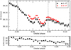 |
Fig. 2 Top panel: ESPRESSO radial velocities of the WASP-121b transits observed. Vertical dotted lines indicate the expected beginning and end of the transit. Bottom panel: RV difference between the two transits, calculated by quadratically interpolating the 1-UT RVs on the 4-UT phases. The black line shows the fitted linear trend with a slope significant at the 4.5σ level. An offset is expected because of the different instrumental setups used in the two transits. |
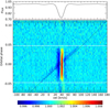 |
Fig. 3 Top panel: average out-of-transit stellar CCF. Bottom panel: tomography of CCF residuals for the 1-UT transit, in the stellar restframe. The stellar systemic velocity Vsys is still not subtracted. Horizontal white lines represent the beginning and end of the transit. The dotted black line shows the theoretical planetary RV. Differences between the stellar CCF residuals before and after the transit, possibly due to stellar activity, are noticeable. |
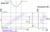 |
Fig. 4 Schematic view of the atmospheric RM effect. |
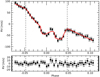 |
Fig. 5 RVs of the 1-UT transit together with the RM + atmospheric RM fit performed. The residuals are shown in the bottom panel. |
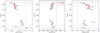 |
Fig. 6 Center (left panel), contrast (central panel), and width (right panel) of the in-transit atmospheric CCFs Gaussian fits as a function of the orbital phase. Horizontal blue lines show the transit duration, dashed blue lines show the full-transit limits. Measurements are not done where the atmospheric track is superimposed on the Doppler shadow. |
4.2 Planetary CCF
The planetary atmospheric track shown in Fig. 3 is slightly shifted from the theoretical planetary velocity computed with the orbital parameters of Table 2. ESPRESSO has recently proven its capability to resolve time variations of this atmospheric track (Ehrenreich et al. 2020). For WASP-121b, Bourrier et al. (2020a) found a similar behavior. We thus investigated this with our data, by fitting a Gaussian profile to each atmospheric line profile in the planetary restframe. Errors on the CCF residuals were set to the standard deviation of their continuum. We excluded the part of the transit where the atmospheric track overlaps the Doppler shadow (see Ehrenreich et al. 2020). The results are shown in Fig. 6. The velocity center of the atmospheric track changes with time (Fig. 6, left panel), becoming more blueshifted in the second part of the transit, in a way similar to what happens in the case of the ultra-hot gas giant WASP-76b (Ehrenreich et al. 2020). This is confirmed by the agreement between the 1-UT and 4-UT data, unfortunately only possible for the second part of the transit. We measure an average change in blueshift from − 2.80 ± 0.28 km s−1 in the first half to − 7.66 ± 0.16 km s−1 in the second half, excluding the ingress and egress. The results are close to those of Bourrier et al. (2020a), who discovered that the atmospheric signal was becoming more blueshifted from the first to the second part of the transit. While we find no differences in the atmospheric CCF contrast (1050 ± 80 versus 970 ± 30 ppm), its width increases but not significantly (7.3 ± 0.7 versus 10.2 ± 0.4 km s−1). The contrasts can be translated into an effective planetary radius of ~ 1.03 Rp (see details in Sect. 6), which is in agreement with the Ratmo found with the RV analysis (Ratmo = 1.052 ± 0.015Rp), thus reinforcing the validity of the atmospheric RM method. The average blueshift values found with the two analyses are also consistent with each other.
5 Transmission spectrum
The transmission spectrum is extracted following basically the procedure of Wyttenbach et al. (2015), which was performed independently for each of the two transits. We first shift the spectra to the stellar restframe by using the Keplerian model of the system with the parameters of Table 2, then we normalized each spectrum. Telluric correction is performed by exploiting the scaling relation between airmass and telluric line strength (Snellen et al. 2008; Vidal-Madjar et al. 2010; Astudillo-Defru & Rojo 2013), rescaling all the spectra as if they were observed to the airmass of the transit center. We can perform telluric correction in the stellar restframe as the variation of the Barycentric Earth RVs during one night is well below the resolution of the instrument. Then we divided all the spectra by a master stellar spectrum created by averaging all the out-of-transit spectra. At this stage we find in the residual spectra a clear pattern of wiggles, which was already described inTabernero et al. (2020). We correct for this pattern by fitting for a sinusoid with varying period, phase, and amplitude for each spectrum, with the fit performed independently for each wavelength region where we looked for spectral features. As a final step, we move to the planetary restframe by shifting all the residual spectra for the theoretical planetary radial velocity (calculated with values from Table 2). The transmission spectrum is now created by averaging all the full-in-transit residual spectra. We note again that the spectral resolution is different for the two transits analyzed. In order to take this into account when estimating the significance of the detections in the transmission spectrum, the final rebinning is done with a wavelength step of 0.01 Å for the 1-UT data and of 0.02 Å for the 4-UT data. These values were chosen because they are very close to the mean resolution step calculated on the whole spectrograph range in the two observing modes.
5.1 Stellar contamination in the transmission spectrum
The star in front of which the planet transits is not a simple homogeneous disk, but rotates and has a surface brightness that changes as afunction of the distance from the center. Effects such as center-to-limb variation (CLV) and stellar rotation bring spurious signals in the transmission spectrum, possibly causing false detections (e.g., Casasayas-Barris et al. 2020) and incorrect line-profile estimations (e.g., Borsa & Zannoni 2018).
For the case of the WASP-121b transmission spectrum, these effects have been proven to be negligible while analyzing HARPS data (Cabot et al. 2020; Bourrier et al. 2020a). Since with ESPRESSO we clearly see their impact in the 4-UT spectra (Fig. 7), we take them into account when analyzing our data. We thus created a model following the methodology of Yan et al. (2017). The star is modeled as a disk divided in sections of 0.01 Rs. For each point we calculate the μ value (μ = cosθ, with θ the angle between the normal to the stellar surface and the considered line of sight) and the projected rotational velocity (by rescaling the v sin i value of Table 2). Then we assign a spectrum to each point of the grid, by quadratically interpolating on μ and Doppler-shifting the model spectra created using the tool Spectroscopy Made Easy (SME, Piskunov & Valenti 2017), with ATLAS9 stellar atmospheric models (assuming solar abundances and local thermodynamic equilibrium approximation) and the line list from the VALD database (Ryabchikova et al. 2015). The model spectra are created for 21 different μ values and with null rotational velocity, and adapted to the resolving power of the instrument. Then we simulate the transit of the planet, calculating for different orbital phases the stellar spectrum as the average spectrum of the non-occulted modeled sections. We divide these for an average out-of-transit stellar spectrum, and we have as a result the simulated RM+CLV effects at each in-transit orbital phase. In Fig. 7 (right panel), we show in a 2D tomographic map the correction with our model applied to the 4-UT data in the wavelength zone of the sodium D doublet. We can calculate the impact on the average transmission spectrum by moving all the in-transit spectra in the planetary restframe and averaging them.
During the transit of a planet the occulted stellar regions are different. This means that the analysis of planetary transmission spectra which are calculated from complete or incomplete transits will be affected in a different way by the CLV and RM effects. In Fig. 8, we show their impact on the sodium D doublet wavelength region of the two ESPRESSO transmission spectra analyzed. The system orbital configuration makes the global effect larger by a factor ~ 2 for the 4-UT partial transit.
We note that Cabot et al. (2020) showed the non-impact of stellar effects CLV+RM on the transmission spectrum of WASP-121bretrieved using three HARPS transits. Our model is consistent with theirs, but given the higher quality of our ESPRESSO data (and in particular the high S/N of the 4-UT transit; see Fig. 7) we chose to remove stellar effects from the data. For uniformity in the analysis, we subtracted the CLV+RM model from the transmission spectra of both transits.
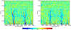 |
Fig. 7 Tomographic map of the sodium D doublet in the planetary restframe for the 4-UT transit, shown before (left panel) and after (right panel) the correction for the CLV and RM effects. The horizontal white line shows the end of the transit; the vertical dashed lines represent the planetary restframe of the sodium D lines. |
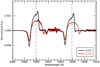 |
Fig. 8 Impact of CLV+RM effects on the transmission spectra of 1-UT (red line) and 4-UT (black line) observed transits in the wavelength region of the sodium D doublet. |
5.2 Detections of planetary absorption lines
We analyzed the transmission spectra retrieved in the two transits independently after the correction of the stellar RM + CLV effects because of the different resolving power of the two observing modes used and because of the difference inthe stellar activity level (Sect. 3.2). A summary of the absorption lines detected in the planetary atmosphere is reported in Table 4. The parameters are calculated with a Gaussian fit and a MCMC error bar estimation. We report from the analysis of the two transits significant detections (> 4σ) for the previously detected Na D1, Na D2, and Hα lines (Fig. 9), together with new detections of Ca II H&K (Fig. 10). Only in the 4-UT transit we can also detect Li, Mg I, and K (Fig. 11). We can detect only one line of the K doublet at ~ 770 nm (Table 4), as the other one falls in a region of very strong telluric absorption. The Mg triplet is detected only when averaging the three lines in the velocity space. We also report on possible detections of Hβ (3.2σ) and Mn triplet (3.3σ) (Fig. 12).
Checking the reference frame of the detections is mandatory when we want to be sure they are caused by the planetary atmosphere and not by spurious stellar effects (e.g., Brogi et al. 2016; Borsa & Zannoni 2018). For each element we thus also report whether the detection is resolved in the 2D tomographic map (Table 4 and Fig. 13). This quality check confirms that the absorption is in the planetary restframe for all the significant detections except for K, which is in a wavelength region particularly affected by strong telluric contamination and so its restframe cannot be discriminated in the 2D map.
Each element line detected in the transmission spectra presents a net blueshift, that for the low layers of the atmosphere (thus excluding Ca II H&K and Hα lines) on average is of ~ –5 km s−1, which is indicative of winds in the planetary atmosphere coming from the dayside to the nightside.
Summary of the detections in the transmission spectra of the two transits.
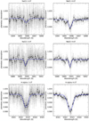 |
Fig. 9 Detections of Na D1 (first row), Na D2 (second row), and Hα (third row) for the transits observed with 1-UT (first column) and 4-UT (second column). The vertical scale is the same for each row, showing the precision of the 4-UT data. The black points represent 0.1 Å binning; theblue line is the best fit Gaussian profile. The vertical dotted line shows the expected planetary restframe. |
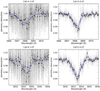 |
Fig. 10 New detections of Ca II H (first row) and Ca II K (second row) in the 1-UT and 4-UT transits (first and second column, respectively). The black points represent 0.1 Å binning; the blue line is the best fit Gaussian profile. The vertical dotted line shows the expected planetary restframe. |
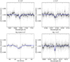 |
Fig. 11 New detections of K (top left), Li (top right), and Mg (bottom panels) in the 4-UT transit. The black points represent 0.1Å (5 km s−1 for Mg triplet) binning; the blue line is the best fit Gaussian profile. The vertical dotted line shows the expected planetary restframe. |
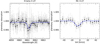 |
Fig. 12 Possible detections of Hβ and Mn triplet (averaged in the velocity space) planetary line profiles in the 4-UT transmission spectrum. The black points represent 0.1Å binning (5 km s−1 for Mn); the blue line is the best fit Gaussian profile. The vertical dotted line shows the expected planetary restframe. |
5.3 Cross-correlation with templates
We created WASP-121b high-resolution theoretical transmission spectra, expressed in planetary radius as a function of wavelength for different species of interest. Models of Fe I, Fe II, Ti I, Ti II, Cr I, V I, TiO (Plez linelist), and VO (Plez linelist) were generated by using petitRADTRANS (Mollière et al. 2019), while those of CaH and ZrO were generated via TURBOSPECTRUM (Plez 2012). We assumed solar abundances, an isothermal atmospheric profile with T = 3000 K and a continuum pressure level of 1 mbar. These parameters were set because they are typical for UHJs (e.g., Hoeijmakers et al. 2019; Stangret et al. 2020). The atmospheric models were translated into flux (Rp ∕Rs)2, convolved at the ESPRESSO resolving power and continuum normalized.
Cross-correlation between the data and the models is performed in the stellar restframe on single residual spectra after the removal of amaster out-of-transit star and telluric contamination (with the procedures explained in Sect. 5) over the whole ESPRESSO wavelength range. We define the cross-correlation as
 (1)
(1)
where M is the model normalized to unity and x are the N wavelengths of the spectra taken at the time t and shifted at the velocity v. In this way, we preserve the flux information (e.g., Hoeijmakers et al. 2019). In our analysis we set to zero all the model lines with contrast of less than 5% of the maximum in our wavelength range.
We selected a step of 0.5 km s−1 (1 km s−1 for the 4-UT) and a velocity range [−200, 200] km s−1. The spectra are divided into segments of 200 Å (see, e.g., Hoeijmakers et al. 2019), then the cross-correlation is performed for each segment. We performed a sigma-clipping at 5σ and masked the wavelength ranges most affected by telluric contamination (the intervals 5240–5280, 6865–6930, 7580–7700 Å). Then for each exposure we applied a weighted average between the cross-correlations of the single segments, where the weights applied to each segment are the inverse of its standard deviation (i.e., since we are in the photon-noise dominated regime, the higher the S/N, the greater the weight) and the depths of the lines in the model. For a range of Kp values from 0 to 300 km s−1, in steps of 1 km s−1, we averaged the in-transit cross-correlation functions after shifting them in the planetary restframe. This is done by subtracting the planetary radial velocity calculated for each spectrum as vp = Kp × sin2πϕ, with ϕ the orbital phase. We thus created the Kp versus Vsys maps that are used to verify the real planetary origin of any possible signal. We evaluated the noise by calculating the standard deviation of the Kp versus Vsys maps, where |V | > 70 km s−1, i.e., far fromwhere any stellar or planetary signal is expected. The significance of the detections (Table 5) was calculated by dividing the best Kp cross-correlation function for the noise, and by fitting a Gaussian function to the result.
We confirm previous detections of Fe I (Fig. 14), Cr I (Fig. 15), and V I (Fig. 16). We also confirm the presence of Fe II in the planetary atmosphere (Fig. 17), which has been previously debated (Ben-Yami et al. 2020; Hoeijmakers et al. 2020). A net blueshift is present for all the detections. We find no evidence of the presence of Ti I (66 ppm at 3σ), Ti II (460 ppm), VO (18 ppm), TiO (12 ppm), CaH (36 ppm), or ZrO (20 ppm), given the accuracy of the linelists used.
In Table 5, we present a summary of the detections in the two transits. The best Kp is often lower than the theoretical value (Kp ~ 218 km s−1). This is possibly due to the atmospheric blueshift variability discussed in Sect. 4.2. It is interesting to note that while for Fe I, Fe II, and V I the detection significance (calculated at the theoretical Kp) is higher forthe complete 1-UT transit (with no detection of Fe II with the 4-UT), it is the opposite for the case of Cr I. We recall that the two datasets were acquired with different resolving power (R ~ 140 000 for 1-UT versus R ~ 70 000 for 4-UT). We also note that the efficiency of the two observing modes is different, and in particular the transits were observed before the fiber upgrade (Pepe et al. 2020). It is hard in this case to make a direct comparison of what is better between resolving power and S/N when looking for species by using the cross-correlation technique since the two datasets are not compatible due to the incompleteness of the 4-UT transit. It is probable, however, that a combination of the two variables is a key factor, depending also on which wavelength region the lines of the species that are searched for fall into.
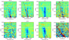 |
Fig. 13 Tomography positive quality checks of the detections in the planetary restframe, for the 4-UT partial transit, before applying the stellar contamination correction (this also shows the restframe of the Doppler shadow, i.e., the red track). Each square represents a 0.1 Å bin on the horizontal scale (except 0.2 Å for Li and 1 km s−1 for Mg). The color scale (not shown here as these are qualitative plots) is different for each plot, from blue representing absorption to red representing emission. The vertical dotted lines represent the laboratory wavelength. The horizontal white lines represent the end of the transit. The Mg tomography (bottom right plot) is presented in the velocity space as the sum of the three lines of the triplet. |
Summary of cross-correlation detections in the atmosphere of WASP-121b, with results for the 1-UT and 4-UT transits.
6 Discussion and conclusions
We observed two transits of the UHJ WASP-121b with ESPRESSO. By analyzing the strange shape of the in-transit RVs, we were able to prove that this is a case of atmospheric RM, showing the presence of (mostly) Fe in the planetary atmosphere and its blueshift by using only the stellar RVs. The atmospheric RM is confirmed to be a valid way to detect in the atmosphere of exoplanets lines that are present in the stellar mask used to calculate the RVs. By studying the exoplanet transmission spectrum, we more than doubled the number of previously detected atomic species in the atmosphere of WASP-121b, reinforcing previous detections of Na D1, Na D2, and Hα, and adding Li, Mg, K, and Ca II H&K (and possibly Hβ and Mn). Lithium detection, despite its low amplitude (~0.2%), is significantat >6σ level. This is a remarkable result, considering that it is achieved with only one partial transit with the 4-UT mode and we were able to confirm it in the planetary restframe with the 2D tomography. This became possible thanks also to the fact that there is no lithium line in the stellar spectrum, thus we are working at the continuum level with a very high S/N. Lithium was first claimed in an exoplanetary atmosphere by Chen et al. (2018) for WASP-127b, but with low-resolution transmission spectroscopy (and not confirmed with high resolution, Allart et al. 2020). Tabernero et al. (2020) and this work present the first detections of Li in planetary atmospheres at high resolution, also providing 2D tomographic evidence of their coherence with the planetary restframe. The detection of a trace element like Li in exoplanet atmospheres is an important step, as it can help in the understanding of planet formation history and lithium depletion in planet-hosting stars (e.g., Bouvier 2008; Israelian et al. 2009; Chen et al. 2018). We note that we cannot detect lithium in the 1-UT transit because of the insufficient S/N.
In Fig. 18, we show the effective planet radius for the detected elements, which is calculated assuming  , where δ is the transit depth (from Table 2) and h is the line contrast (e.g., Chen et al. 2020). As expected, features like Ca II and Hα are present up to very high altitudes in the atmosphere, as in the case of other hot exoplanets (e.g., Yan & Henning 2018; Yan et al. 2019; Casasayas-Barris et al. 2019). The absorptions from Ca II H&K lines are very prominent, probing atmospheric layers close to and possibly beyond the planetary Roche radius (RRoche ~ 1.77Rp). As the Roche lobe is elongated toward the star, in a transiting configuration it extends to about two-thirds of the extension to the L1 Lagrange point (Vidal-Madjar et al. 2008), with an equivalent value of the transiting Roche lobe of ~ 1.3 Rp for WASP-121b (Sing et al. 2019). Ionized species were already detected at these high altitudes in the atmosphere of WASP-121b with HST (Fe II and Mg II, Sing et al. 2019). When considering the equivalent Roche lobe radius, our detections of Ca II H&K and also Hα are significantly beyond it at the 5.3σ, 5.9σ, and 6.2σ level, respectively, for the case of the 4-UT transit. We note that the model spectra we used for the CLV + RM effect correction could be imperfect in the core of chromospheric lines such as Ca II H&K (e.g., Casasayas-Barris et al. 2020). However, the presence of strong absorption in the planet atmosphere is certain as it is also confirmed by the 2D tomographic map (Fig. 13). The slight asymmetries observed on these line profiles (Fig. 10) could be due to the extension beyond the Roche lobe radius, and thus could be probing an ongoing planetary atmospheric escape.
Our detections probe different layers of the atmosphere, thus we compared the retrieved line widths to those predicted for a tidally locked WASP-121b (Fig. 19). While for the low atmosphere tidally locked rotation can account for most of the thermal broadening (also pointed out in Bourrier et al. 2020a), the full width at half maximum (FWHM) values of the deepest absorption lines Hα and Ca II are significantly larger than those expected for a tidally locked rotating atmosphere. Tidally locked rotation is thus not the main source of atmospheric broadening for the higher layers of the atmosphere. In addition, the blueshift of Ca II H&K is larger than for the other detected lines. The planet is probably experiencing atmospheric evaporation, thus the lines could be broadened by the expanding atmosphere via vertical winds or high-altitude jets (Seidel et al. 2020; Wyttenbach et al. 2020).
We note that the line contrast of the detected atmospheric features is systematically (but not significantly) higher for the 4-UTdata with respect to the 1-UT (Table 4, Fig. 18). This is hardly due to the different spectral resolution, as in this case we would expect an opposite behavior (i.e., lines becoming deeper with higher resolving power). One possible cause is the atmospheric blueshift variability during transit shown in Sect. 4.2. This in fact causes a spread of the lines when we sum all the single transmission spectra of the 1-UT transit. On the contrary, this does not happen for the 4-UT data, as they are restricted to the second part of the full transit where the atmospheric restframe is almost constant (Fig. 6, left panel). One more possible interesting explanation could be the different level of stellar activity during the two transits, with the star being more active when we observe deeper planetary atmospheric lines. The contrast difference is seen for lines that are sensitive to stellar activity such as Na D, Hα, and Ca II H&K. We do not know exactly the timescales necessary for the atmosphere to react to stellar activity changes, but the temporal distance of >1 month between the two observed transits could be more than enough.
With one partial transit with the 4-UT MR mode we could detect more elements than with one complete transit with the 1-UT HR mode. This is due to the very high S/N of the 4-UT data, which exploits the light coming from a 16m-equivalent telescope despite the lower resolving power (R ~ 70 000 versus R ~ 138 000). In this case the S/N overcomes the spectral resolution when looking for single lines of atomic species.
In conclusion, ESPRESSO is able to deeply investigate the atmospheres of exoplanets and temporally resolve the atmospheric behavior; it will play a major role in the coming years in the field of exoplanet characterization. Here, we showed its potential applied to the atmospheric analysis of WASP-121b, which is confirmed to be one of the most intriguing UHJs and that definitely deserves future follow-up investigations.
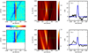 |
Fig. 14 Cross-correlation of the data with the Fe I model. Shown are the results for the 1-UT transit (top), and those for the 4-UT transit (bottom). The first column shows the contour plots of the temporal variation of the cross-correlation, with a dashed line to show the expected planetary velocity; the colorbar scale is in ppm. The second column is the Kp versus velocity map after summing the cross-correlations for different Kp, with colorbar scale in S/N. Green dashed lines are centered on the expected planetary position. The third column shows the final S/N of the detection, with the performed Gaussian fit in blue, as calculated at the theoretical Kp value. |
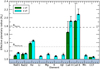 |
Fig. 18 Effective planetary radius for each element detected, shown for both the transits analyzed. Error bars refer to 1σ. The horizontal dashed and dotted lines represent respectively the Roche lobe radius of 1.77 Rp and the transit-equivalent Roche lobe radius for the transiting exoplanet case of ~ 1.3 Rp. |
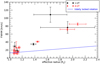 |
Fig. 19 Effective planetary radius vs FWHMs of the elements detected. The blue line shows the expected tidally locked planet’s rotational broadening. |
Acknowledgements
We thank the referee for their useful comments that helped improving the clarity of the manuscript. The authors acknowledge the ESPRESSO project team for its effort and dedication in building the ESPRESSO instrument. FB acknowledges financial support from INAF through the ASI-INAF contract 2015-019-R0, and M. Rainer for helpful discussions on the Fourier transform of the CCF. This work has been carried out within the framework of the National Centre of Competence in Research PlanetS supported by the Swiss National Science Foundation. R.A. acknowledge the financial support of the SNSF. This work was supported by FCT – Fundação para a Ciência e a Tecnologia through national funds and by FEDER through COMPETE2020 – Programa Operacional Competitividade e Internacionalização by these grants: UID/FIS/04434/2019; UIDB/04434/2020; UIDP/04434/2020; PTDC/FIS-AST/32113/2017 & POCI-01-0145-FEDER-032113; PTDC/FIS-AST/28953/2017 & POCI-01-0145-FEDER-028953; PTDC/FIS-AST/28987/2017 & POCI-01-0145-FEDER-028987. O.D.S.D. is supported in the form of work contract (DL 57/2016/CP1364/CT0004) funded by FCT. This project has received funding from the European Research Council (ERC) under the European Union’s Horizon 2020 research and innovation programme (project Four Aces grant agreement no. 724427). This work has made use of data from the European Space Agency (ESA) mission Gaia (https://www.cosmos.esa.int/gaia), processed by the Gaia Data Processing and Analysis Consortium (DPAC, https://www.cosmos.esa.int/web/gaia/dpac/consortium). Funding for the DPAC has been provided by national institutions, in particular the institutions participating in the Gaia Multilateral Agreement.
References
- Allart, R., Pino, L., Lovis, C., et al. 2020, A&A, 644, A155 [NASA ADS] [CrossRef] [EDP Sciences] [Google Scholar]
- Astudillo-Defru, N., & Rojo, P. 2013, A&A, 557, A56 [NASA ADS] [CrossRef] [EDP Sciences] [Google Scholar]
- Astudillo-Defru, N., Delfosse, X., Bonfils, X., et al. 2017, A&A, 600, A13 [NASA ADS] [CrossRef] [EDP Sciences] [Google Scholar]
- Ben-Yami, M., Madhusudhan, N., Cabot, S. H. C., et al. 2020, ApJ, 897, L5 [CrossRef] [Google Scholar]
- Borsa, F., & Zannoni, A. 2018, A&A, 617, A134 [NASA ADS] [CrossRef] [EDP Sciences] [Google Scholar]
- Borsa, F., Scandariato, G., Rainer, M., et al. 2015, A&A, 578, A64 [NASA ADS] [CrossRef] [EDP Sciences] [Google Scholar]
- Borsa, F., Rainer, M., Bonomo, A. S., et al. 2019, A&A, 631, A34 [NASA ADS] [CrossRef] [EDP Sciences] [Google Scholar]
- Bourrier, V., & des Etangs, A. L. 2018, Handbook of Exoplanets, 148 [Google Scholar]
- Bourrier, V., Ehrenreich, D., Lendl, M., et al. 2020a, A&A, 635, A205 [NASA ADS] [CrossRef] [EDP Sciences] [Google Scholar]
- Bourrier, V., Kitzmann, D., Kuntzer, T., et al. 2020b, A&A, 637, A36 [CrossRef] [EDP Sciences] [Google Scholar]
- Bouvier, J. 2008, A&A, 489, L53 [NASA ADS] [CrossRef] [EDP Sciences] [Google Scholar]
- Brogi, M., de Kok, R. J., Albrecht, S., et al. 2016, ApJ, 817, 106 [Google Scholar]
- Brogi, M., Line, M., Bean, J., et al. 2017, ApJ, 839, L2 [NASA ADS] [CrossRef] [Google Scholar]
- Brown, D. J. A., Triaud, A. H. M. J., Doyle, A. P., et al. 2017, MNRAS, 464, 810 [Google Scholar]
- Cabot, S. H. C., Madhusudhan, N., Welbanks, L., et al. 2020, MNRAS, 494, 363 [NASA ADS] [CrossRef] [Google Scholar]
- Casasayas-Barris, N., Palle, E., Nowak, G., et al. 2017, A&A, 608, A135 [NASA ADS] [CrossRef] [EDP Sciences] [Google Scholar]
- Casasayas-Barris, N., Pallé, E., Yan, F., et al. 2019, A&A, 628, A9 [NASA ADS] [CrossRef] [EDP Sciences] [Google Scholar]
- Casasayas-Barris, N., Palle, E., Yan, F., et al. 2020, A&A, 635, A206 [NASA ADS] [CrossRef] [EDP Sciences] [Google Scholar]
- Chen, G., Pallé, E., Welbanks, L., et al. 2018, A&A, 616, A145 [NASA ADS] [CrossRef] [EDP Sciences] [Google Scholar]
- Chen, G., Casasayas-Barris, N., Pallé, E., et al. 2020, A&A, 635, A171 [CrossRef] [Google Scholar]
- Delrez, L., Santerne, A., Almenara, J.-M., et al. 2016, MNRAS, 458, 4025 [NASA ADS] [CrossRef] [Google Scholar]
- Deming, L. D., & Seager, S. 2017, J. Geophys. Res. (Planets), 122, 53 [NASA ADS] [CrossRef] [Google Scholar]
- Di Gloria, E., Snellen, I. A. G., & Albrecht, S. 2015, A&A, 580, A84 [NASA ADS] [CrossRef] [EDP Sciences] [Google Scholar]
- Dravins, D., Lindegren, L., & Torkelsson, U. 1990, A&A, 237, 137 [NASA ADS] [Google Scholar]
- Dreizler, S., Reiners, A., Homeier, D., et al. 2009, A&A, 499, 615 [NASA ADS] [CrossRef] [EDP Sciences] [Google Scholar]
- Eastman, J., Gaudi, B. S., & Agol, E. 2013, PASP, 125, 923 [Google Scholar]
- Ehrenreich, D., Lovis, C., Allart, R., et al. 2020, Nature, 580, 597 [Google Scholar]
- Evans, T. M., Sing, D. K., Kataria, T., et al. 2017, Nature, 548, 58 [NASA ADS] [CrossRef] [Google Scholar]
- Evans, T. M., Sing, D. K., Goyal, J. M., et al. 2018, AJ, 156, 283 [NASA ADS] [CrossRef] [Google Scholar]
- Faria, J. P., Adibekyan, V., Amazo-Gómez, E. M., et al. 2020, A&A, 635, A13 [NASA ADS] [CrossRef] [EDP Sciences] [Google Scholar]
- Fossati, L., Haswell, C. A., Froning, C. S., et al. 2010, ApJ, 714, L222 [Google Scholar]
- Gaia Collaboration 2018, VizieR Online Data Catalog, I/345 [Google Scholar]
- Gibson, N. P., Merritt, S., Nugroho, S. K., et al. 2020, MNRAS, 493, 2215 [Google Scholar]
- Gustafsson, B., Edvardsson, B., Eriksson, K., et al. 2008, A&A, 486, 951 [NASA ADS] [CrossRef] [EDP Sciences] [Google Scholar]
- Hoeijmakers, H. J., Ehrenreich, D., Heng, K., et al. 2018, Nature, 560, 453 [NASA ADS] [CrossRef] [Google Scholar]
- Hoeijmakers, H. J., Ehrenreich, D., Kitzmann, D., et al. 2019, A&A, 627, A165 [NASA ADS] [CrossRef] [EDP Sciences] [Google Scholar]
- Hoeijmakers, H. J., Seidel, J. V., Pino, L., et al. 2020, A&A, 641, A123 [CrossRef] [Google Scholar]
- Israelian, G., Delgado Mena, E., Santos, N. C., et al. 2009, Nature, 462, 189 [NASA ADS] [CrossRef] [PubMed] [Google Scholar]
- Kovács, G., & Kovács, T. 2019, A&A, 625, A80 [NASA ADS] [CrossRef] [EDP Sciences] [Google Scholar]
- Lothringer, J. D., Barman, T., & Koskinen, T. 2018, ApJ, 866, 27 [NASA ADS] [CrossRef] [Google Scholar]
- McLaughlin, D. B. 1924, ApJ, 60, 22 [Google Scholar]
- Merritt, S. R., Gibson, N. P., Nugroho, S. K., et al. 2020, A&A, 636, A117 [CrossRef] [EDP Sciences] [Google Scholar]
- Mikal-Evans, T., Sing, D. K., Goyal, J. M., et al. 2019, MNRAS, 488, 2222 [Google Scholar]
- Mollière, P., Wardenier, J. P., van Boekel, R., et al. 2019, A&A, 627, A67 [NASA ADS] [CrossRef] [EDP Sciences] [Google Scholar]
- Noyes, R. W., Hartmann, L. W., Baliunas, S. L., et al. 1984, ApJ, 279, 763 [NASA ADS] [CrossRef] [Google Scholar]
- Ohta, Y., Taruya, A., & Suto, Y. 2005, ApJ, 622, 1118 [Google Scholar]
- Oshagh, M., Triaud, A. H. M. J., Burdanov, A., et al. 2018, A&A, 619, A150 [NASA ADS] [CrossRef] [EDP Sciences] [Google Scholar]
- Parmentier, V., Line, M. R., Bean, J. L., et al. 2018, A&A, 617, A110 [NASA ADS] [CrossRef] [EDP Sciences] [Google Scholar]
- Pepe, F. A., Cristiani, S., Rebolo Lopez, R., et al. 2010, Proc. SPIE, 77350F [CrossRef] [Google Scholar]
- Pepe, F., Molaro, P., Cristiani, S., et al. 2014, Astron. Nachr., 335, 8 [Google Scholar]
- Pepe, F., Cristiani, S., Rebolo, R., et al. 2020, A&A, in press, https://doi.org/10.1051/0004-6361/202038306 [Google Scholar]
- Piskunov, N., & Valenti, J. A. 2017, A&A, 597, A16 [NASA ADS] [CrossRef] [EDP Sciences] [Google Scholar]
- Plez, B. 2012, Astrophysics Source Code Library [record ascl:1205.004] [Google Scholar]
- Reiners, A., & Schmitt, J. H. M. M. 2002, A&A, 384, 155 [NASA ADS] [CrossRef] [EDP Sciences] [Google Scholar]
- Reiners, A., Schmitt, J. H. M. M. 2003, A&A, 398, 647 [NASA ADS] [CrossRef] [EDP Sciences] [Google Scholar]
- Rossiter, R. A. 1924, ApJ, 60, 15 [Google Scholar]
- Ryabchikova, T., Piskunov, N., Kurucz, R. L., et al. 2015, Phys. Scr, 90, 054005 [NASA ADS] [CrossRef] [Google Scholar]
- Salz, M., Schneider, P. C., Fossati, L., et al. 2019, A&A, 623, A57 [NASA ADS] [CrossRef] [EDP Sciences] [Google Scholar]
- Seager, S., & Mallén-Ornelas, G. 2003, ApJ, 585, 1038 [NASA ADS] [CrossRef] [Google Scholar]
- Seidel, J. V., Ehrenreich, D., Pino, L., et al. 2020, A&A, 633, A86 [NASA ADS] [CrossRef] [EDP Sciences] [Google Scholar]
- Serrano, L. M., Oshagh, M., Cegla, H. M., et al. 2020, MNRAS, 493, 5928 [CrossRef] [Google Scholar]
- Sing, D. K., Lavvas, P., Ballester, G. E., et al. 2019, AJ, 158, 91 [Google Scholar]
- Snellen, I. A. G. 2004, MNRAS, 353, L1 [Google Scholar]
- Snellen, I. A. G., Albrecht, S., de Mooij, E. J. W., & Le Poole, R. S. 2008, A&A, 487, 357 [NASA ADS] [CrossRef] [EDP Sciences] [Google Scholar]
- Snellen, I. A. G., de Kok, R. J., de Mooij, E. J. W., et al. 2010, Nature, 465, 1049 [NASA ADS] [CrossRef] [PubMed] [Google Scholar]
- Stangret, M., Casasayas-Barris, N., Pallé, E., et al. 2020, A&A, 638, A26 [CrossRef] [EDP Sciences] [Google Scholar]
- Tabernero, H. M., Dorda, R., Negueruela, I., et al. 2018, MNRAS, 476, 3106 [Google Scholar]
- Tabernero, H. M., Marfil, E., Montes, D., et al. 2019, A&A, 628, A131 [CrossRef] [EDP Sciences] [Google Scholar]
- Tabernero, H. M., Zapatero Osorio, M. R., Allart, R., et al. 2020, A&A, in press, https://doi.org/10.1051/0004-6361/202039511 [Google Scholar]
- Ter Braak, C. J. F. 2006, Statist. Comput., 16, 239 [CrossRef] [Google Scholar]
- Vidal-Madjar, A., Lecavelier des Etangs, A., Désert, J.-M., et al. 2003, Nature, 422, 143 [Google Scholar]
- Vidal-Madjar, A., Lecavelier des Etangs, A., Désert, J.-M., et al. 2008, ApJ, 676, L57 [NASA ADS] [CrossRef] [Google Scholar]
- Vidal-Madjar, A., Arnold, L., Ehrenreich, D., et al. 2010, A&A, 523, A57 [NASA ADS] [CrossRef] [EDP Sciences] [Google Scholar]
- Winn, J. N., Johnson, J. A., Narita, N., et al. 2008, ApJ, 682, 1283 [NASA ADS] [CrossRef] [Google Scholar]
- Wyttenbach, A., Ehrenreich, D., Lovis, C., et al. 2015, A&A, 577, A62 [NASA ADS] [CrossRef] [EDP Sciences] [Google Scholar]
- Wyttenbach, A., Mollière, P., Ehrenreich, D., et al. 2020, A&A, 638, A87 [EDP Sciences] [Google Scholar]
- Yan, F., & Henning, T. 2018, Nat. Astron., 2, 714 [NASA ADS] [CrossRef] [Google Scholar]
- Yan, F., Pallé, E., Fosbury, R. A. E., et al. 2017, A&A, 603, A73 [NASA ADS] [CrossRef] [EDP Sciences] [Google Scholar]
- Yan, F., Casasayas-Barris, N., Molaverdikhani, K., et al. 2019, A&A, 632, A69 [NASA ADS] [CrossRef] [EDP Sciences] [Google Scholar]
Publicly available at www.eso.org/sci/software/pipelines/espresso/espresso-pipe-recipes.html
All Tables
Summary of cross-correlation detections in the atmosphere of WASP-121b, with results for the 1-UT and 4-UT transits.
All Figures
|
Fig. 1
|
| In the text | |
|
Fig. 2 Top panel: ESPRESSO radial velocities of the WASP-121b transits observed. Vertical dotted lines indicate the expected beginning and end of the transit. Bottom panel: RV difference between the two transits, calculated by quadratically interpolating the 1-UT RVs on the 4-UT phases. The black line shows the fitted linear trend with a slope significant at the 4.5σ level. An offset is expected because of the different instrumental setups used in the two transits. |
| In the text | |
|
Fig. 3 Top panel: average out-of-transit stellar CCF. Bottom panel: tomography of CCF residuals for the 1-UT transit, in the stellar restframe. The stellar systemic velocity Vsys is still not subtracted. Horizontal white lines represent the beginning and end of the transit. The dotted black line shows the theoretical planetary RV. Differences between the stellar CCF residuals before and after the transit, possibly due to stellar activity, are noticeable. |
| In the text | |
|
Fig. 4 Schematic view of the atmospheric RM effect. |
| In the text | |
|
Fig. 5 RVs of the 1-UT transit together with the RM + atmospheric RM fit performed. The residuals are shown in the bottom panel. |
| In the text | |
|
Fig. 6 Center (left panel), contrast (central panel), and width (right panel) of the in-transit atmospheric CCFs Gaussian fits as a function of the orbital phase. Horizontal blue lines show the transit duration, dashed blue lines show the full-transit limits. Measurements are not done where the atmospheric track is superimposed on the Doppler shadow. |
| In the text | |
|
Fig. 7 Tomographic map of the sodium D doublet in the planetary restframe for the 4-UT transit, shown before (left panel) and after (right panel) the correction for the CLV and RM effects. The horizontal white line shows the end of the transit; the vertical dashed lines represent the planetary restframe of the sodium D lines. |
| In the text | |
|
Fig. 8 Impact of CLV+RM effects on the transmission spectra of 1-UT (red line) and 4-UT (black line) observed transits in the wavelength region of the sodium D doublet. |
| In the text | |
|
Fig. 9 Detections of Na D1 (first row), Na D2 (second row), and Hα (third row) for the transits observed with 1-UT (first column) and 4-UT (second column). The vertical scale is the same for each row, showing the precision of the 4-UT data. The black points represent 0.1 Å binning; theblue line is the best fit Gaussian profile. The vertical dotted line shows the expected planetary restframe. |
| In the text | |
|
Fig. 10 New detections of Ca II H (first row) and Ca II K (second row) in the 1-UT and 4-UT transits (first and second column, respectively). The black points represent 0.1 Å binning; the blue line is the best fit Gaussian profile. The vertical dotted line shows the expected planetary restframe. |
| In the text | |
|
Fig. 11 New detections of K (top left), Li (top right), and Mg (bottom panels) in the 4-UT transit. The black points represent 0.1Å (5 km s−1 for Mg triplet) binning; the blue line is the best fit Gaussian profile. The vertical dotted line shows the expected planetary restframe. |
| In the text | |
|
Fig. 12 Possible detections of Hβ and Mn triplet (averaged in the velocity space) planetary line profiles in the 4-UT transmission spectrum. The black points represent 0.1Å binning (5 km s−1 for Mn); the blue line is the best fit Gaussian profile. The vertical dotted line shows the expected planetary restframe. |
| In the text | |
|
Fig. 13 Tomography positive quality checks of the detections in the planetary restframe, for the 4-UT partial transit, before applying the stellar contamination correction (this also shows the restframe of the Doppler shadow, i.e., the red track). Each square represents a 0.1 Å bin on the horizontal scale (except 0.2 Å for Li and 1 km s−1 for Mg). The color scale (not shown here as these are qualitative plots) is different for each plot, from blue representing absorption to red representing emission. The vertical dotted lines represent the laboratory wavelength. The horizontal white lines represent the end of the transit. The Mg tomography (bottom right plot) is presented in the velocity space as the sum of the three lines of the triplet. |
| In the text | |
|
Fig. 14 Cross-correlation of the data with the Fe I model. Shown are the results for the 1-UT transit (top), and those for the 4-UT transit (bottom). The first column shows the contour plots of the temporal variation of the cross-correlation, with a dashed line to show the expected planetary velocity; the colorbar scale is in ppm. The second column is the Kp versus velocity map after summing the cross-correlations for different Kp, with colorbar scale in S/N. Green dashed lines are centered on the expected planetary position. The third column shows the final S/N of the detection, with the performed Gaussian fit in blue, as calculated at the theoretical Kp value. |
| In the text | |
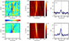 |
Fig. 15 Same as Fig. 14, but for Cr I. |
| In the text | |
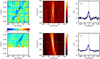 |
Fig. 16 Same as Fig. 14, but for V I. |
| In the text | |
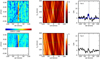 |
Fig. 17 Same as Fig. 14, but for Fe II. |
| In the text | |
|
Fig. 18 Effective planetary radius for each element detected, shown for both the transits analyzed. Error bars refer to 1σ. The horizontal dashed and dotted lines represent respectively the Roche lobe radius of 1.77 Rp and the transit-equivalent Roche lobe radius for the transiting exoplanet case of ~ 1.3 Rp. |
| In the text | |
|
Fig. 19 Effective planetary radius vs FWHMs of the elements detected. The blue line shows the expected tidally locked planet’s rotational broadening. |
| In the text | |
Current usage metrics show cumulative count of Article Views (full-text article views including HTML views, PDF and ePub downloads, according to the available data) and Abstracts Views on Vision4Press platform.
Data correspond to usage on the plateform after 2015. The current usage metrics is available 48-96 hours after online publication and is updated daily on week days.
Initial download of the metrics may take a while.