| Issue |
A&A
Volume 645, January 2021
|
|
|---|---|---|
| Article Number | A66 | |
| Number of page(s) | 32 | |
| Section | Interstellar and circumstellar matter | |
| DOI | https://doi.org/10.1051/0004-6361/202039335 | |
| Published online | 14 January 2021 | |
The fully developed remnant of a neutrino-driven supernova
Evolution of ejecta structure and asymmetries in SNR Cassiopeia A★
1
INAF – Osservatorio Astronomico di Palermo,
Piazza del Parlamento 1,
90134 Palermo,
Italy
e-mail: salvatore.orlando@inaf.it
2
Max-Planck-Institut für Astrophysik,
Karl-Schwarzschild-Str. 1,
85748 Garching, Germany
3
Dip. di Fisica e Chimica, Università degli Studi di Palermo,
Piazza del Parlamento 1,
90134 Palermo, Italy
4
Astrophysical Big Bang Laboratory, RIKEN Cluster for Pioneering Research,
2-1 Hirosawa,
Wako,
Saitama 351-0198, Japan
5
RIKEN Interdisciplinary Theoretical & Mathematical Science Program (iTHEMS),
2-1 Hirosawa,
Wako,
Saitama 351-0198, Japan
Received:
3
September
2020
Accepted:
30
November
2020
Context. The remnants of core-collapse supernovae (SNe) are probes of the physical processes associated with their parent SNe.
Aims. Here we aim to explore to which extent the remnant keeps memory of the asymmetries that develop stochastically in the neutrino-heating layer due to hydrodynamic instabilities (e.g., convective overturn and the standing accretion shock instability; SASI) during the first second after core bounce.
Methods. We coupled a three-dimensional (3D) hydrodynamic model of a neutrino-driven SN explosion, which has the potential to reproduce the observed morphology of the Cassiopeia A (Cas A) remnant, with 3D (magneto)-hydrodynamic simulations of the remnant formation. The simulations cover ≈2000 yr of expansion and include all physical processes relevant to describe the complexities in the SN evolution and the subsequent interaction of the stellar debris with the wind of the progenitor star.
Results. The interaction of large-scale asymmetries left from the earliest phases of the explosion with the reverse shock produces, at the age of ≈350 yr, an ejecta structure and a remnant morphology which are remarkably similar to those observed in Cas A. Small-scale structures in the large-scale Fe-rich plumes that were created during the initial stages of the SN, combined with hydrodynamic instabilities that develop after the passage of the reverse shock, naturally produce a pattern of ring- and crown-like structures of shocked ejecta. The consequence is a spatial inversion of the ejecta layers with Si-rich ejecta being physically interior to Fe-rich ejecta. The full-fledged remnant shows voids and cavities in the innermost unshocked ejecta, which are physically connected with ring-like features of shocked ejecta in the main shell in most cases, resulting from the expansion of Fe-rich plumes and their inflation due to the decay of radioactive species. The asymmetric distributions of 44Ti and 56Fe, which are mostly concentrated in the northern hemisphere, and pointing opposite to the kick velocity of the neutron star, as well as their abundance ratio are both compatible with those inferred from high-energy observations of Chandra and NuSTAR. Finally, the simulations show that the fingerprints of the SN can still be visible ≈2000 yr after the explosion.
Conclusions. The main asymmetries and features observed in the ejecta distribution of Cas A can be explained by the interaction of the reverse shock with the initial large-scale asymmetries that developed from stochastic processes (e.g., convective overturn and SASI activity) that originate during the first seconds of the SN blast.
Key words: hydrodynamics / instabilities / shock waves / ISM: supernova remnants / supernovae: individual: Cassiopeia A / X-rays: ISM
Movies associated to Figs. 7, 8, 12, 15 are available at https://www.aanda.org
© ESO 2021
1 Introduction
Core-collapse supernovae (SNe), the final fate of massive stars, play a major role in the dynamical and chemical evolution of galaxies by driving, for instance, the chemical enrichment and the heating of the diffuse interstellar gas. However, despite the central role played by SNe in the galactic ecosystem, studying the physical processes that govern SN engines is a rather difficult task due to the rarity of these events in our galaxy (about one every ≈50 yr) and due to severe limitations in observations of extragalactic SNe because of their large distances from us. This makes it extremely challenging to extract key information on the explosion processes from observations in the immediate aftermath of an SN, namely when the structure of the rapidly expanding stellar debris keep a full memory of the explosion mechanism.
Nonetheless, there has been a growing consensus in the literature that the fingerprints of SN engines can still be found hundreds to thousands of years after the explosion in the leftover of SNe, the supernova remnants (SNRs). These appear as extended sources which emit both thermal and nonthermal emission in different spectral bands. Spatially resolved spectroscopy has allowed astronomers to investigate in detail the structure of nearby SNRs and the distribution of chemical elements in their interior, revealing the complexity of their morphology and fine-scale ejecta structures that are impossible to observe in unresolved extragalactic sources (e.g., Milisavljevic & Fesen 2017). In a few particular cases, a three-dimensional (3D) reconstruction of the chemical distribution and structure of stellar debris has been possible as, for instance, in the SNRs Cassiopeia A (Cas A; e.g., DeLaney et al. 2010; Milisavljevic & Fesen 2013, 2015; Grefenstette et al. 2014, 2017), SN 1987A (e.g., Abellán et al. 2017; Cigan et al. 2019) and, more recently, N132D (e.g., Law et al. 2020). These studies have revealed very asymmetric distributions of the ejecta that might reflect pristine structures and features of the parent SN explosions, possibly arising from (magneto)-hydrodynamical (MHD or HD) instabilities developed at the launch of the anisotropic blast wave (e.g., Miceli et al. 2006; Lopez et al. 2011; Lopez & Fesen 2018; Holland-Ashford et al. 2020). Particularly relevant are the distributions of radioactive nuclei freshly synthesized during the SN, such as 56Ni and 44Ti, and their decaying products, as 56Co and 56Fe, which originate from the innermost regions of the star where the explosion was launched. Hundreds of years after the SN, these nuclei mightstill encode the fingerprints of the physical processes dominating the earliest phases of the SN in asymmetries that occurred during the explosion, thus allowing us to probe the physics of SN engines.
Information on the explosion dynamics and matter mixing that might be extracted from observations of SNRs can be essential for constraining sophisticated models that describe the complex phases of SN evolution (e.g., Wongwathanarat et al. 2013; Janka et al. 2016; Janka 2017; O’Connor & Couch 2018; Burrows et al. 2019). SN models, however, describe the early phasesfrom the core-collapse up to a timescale of only days, although the age of young nearby SNRs is typically of hundreds of years1, at which age the remnants have interacted with the circumstellar and interstellar medium (CSM and ISM). This makes it very difficult to disentangle the effects of the CSM and ISM interaction on the observed remnant from those of the initial phases of the explosion itself.
A strategy to link observed asymmetries and geometry of the SNR’s bulk ejecta with core-collapse SN simulations is to perform long-term simulations that evolve core-collapse SNe to the age of SNRs (hundreds or thousands of years), and compare the results of these simulations with observations of SNRs. However, this is a rather challenging task that requires a multiscale, multiphysics, and multidimensional approach to describe: the very different temporal and spatial scales involved through the different phases of evolution, the structure and chemical stratification of the progenitor star at collapse, the explosive nucleosynthetic processes, the effects of post-explosion anisotropies (inherently 3D), the interaction of the SNR with the surrounding inhomogeneous (magnetized) medium, and the synthesis of emission in different wavelength bands (necessary for comparison of the model results with observations). The simulations have to follow the entire life cycle of elements from the synthesis in the progenitor star, through the reprocessing by nuclear reactions during the SN, and the subsequent mixing of chemically inhomogeneous layers of the ejecta with the CSM. An additional difficulty stems from the need to disentangle the effects of the SN explosion and of the structure of the progenitor star, from those of the interaction of the blast with the inhomogeneous CSM and ISM. First attempts of long-term 3D MHD or HD simulations confirmed that the above approach is very effective in gaining a deep physical insight of the phenomena that occurred during a SN (e.g., Orlando et al. 2015, 2016, 2019a, 2020; Wongwathanarat et al. 2017; Ferrand et al. 2019, 2021; Ono et al. 2020; Vance et al. 2020; Tutone et al. 2020; Gabler et al. 2020).
Here, we present the complete 3D evolution of a neutrino-driven SN explosion from the core-collapse to the development of its full-fledged remnant interacting with the CSM. To this end, we coupled an elaborate 3D HD model of a neutrino-driven explosion (Wongwathanarat et al. 2017) with state-of-the-art 3D MHD and HD simulations of the remnant formation (Orlando et al. 2016). Going beyond previous studies, the present one represents a significant step forward that allows us to link, for the first time, modeling attempts that have been carried out independently so far, because they are either constrained to the early phase of the SN up to days only (e.g., Wongwathanarat et al. 2017), or starting the long-time remnant evolution with artificial initial conditions (e.g., Orlando et al. 2016). This allowed us to describe the development and evolution of remnant anisotropies self-consistently, as a result of the neutrino-driven mechanism, and to identify ejecta structures of the SNR that encode the imprint of large-scale asymmetries left from the earliest moments of the explosion.
Our study focusses on a SN model that produces a remnant compatible with the observed structure of Cas A, one of the best studied young SNRs of our galaxy (at a distance of ≈ 3.4 kpc; Lee et al. 2014). The 3D structure of Cas A has been characterized in excellent details by multiwavelength observations (e.g., DeLaney et al. 2010; Milisavljevic & Fesen 2013, 2015; Grefenstette et al. 2014, 2017). One of the outstanding characteristics of the Cas A morphology is its overall clumpiness and the presence of large-scale anisotropies (most notably three Fe-rich regions, “crowns” and ring-like structures, voids reaching even into the innermost unshocked ejecta, and Si-rich “sprays” also referred to in the literature as jet-like features). Since observations suggest that the remnant is still expanding through the spherically symmetric wind of the progenitor star (e.g., Lee et al. 2014), the large-scale anisotropies evident in the remnant are most likely due to processes associated to the SN explosion. All the above considerations make Cas A an attractive laboratory for studying the SN-SNR connection. Our aim is to investigate how Cas A’s final morphology reflects the characteristics of the parent SN explosion and, in particular, the asymmetries that developed by nonradial hydrodynamic instabilities connected to the onset of the explosion.
The paper is organized as follows. In Sect. 2 we describe the initial neutrino-driven SN model, the SNR model, and the numerical setup; in Sect. 3 we discuss the results for the modeled structure of the ejecta in the full-fledged remnant in comparison with observations of Cas A; and in Sect. 4 we draw our conclusions; in Appendices A−C, we discuss the effects of radioactive decay and magnetic field on the evolution of the remnant and on the spatial distribution of the ejecta.
2 Problem description and numerical setup
Our computational strategy is analogous to that described in Orlando et al. (2020) and consists in the coupling between elaborate 3D HD models of the SN explosion and state-of-the-art 3D MHD and HD simulations of the remnant formation. For the purpose of the present paper, we considered a core-collapse SN simulation from the blast-wave initiation by the neutrino-driven mechanism, computed until about one day after the SN initiation. This model developed an asymmetric morphological structure that is compatible with that of Cas A (Wongwathanarat et al. 2017). This simulation provided the initial conditions for our 3D SNR simulations soon after the shock breakout (see Sect. 2.1). Then we followed the transition from the early SN phase to the emerging SNR and the subsequent expansion of the remnant through the wind of the stellar progenitor (see Sect. 2.2) as in Orlando et al. (2016).
We notethat our simulations are not expected to reconstruct every detail of the structure of Cas A since the 3D SN model adopted here was selected from a set of models of Wongwathanarat et al. (2015) and no fine-tuning was performed, neither on the progenitor star nor on the explosion properties, to match the morphology and structure of Cas A (see discussion in Wongwathanarat et al. 2017). Nevertheless, our simulations allowed us to investigate if fundamental chemical, physical, geometric properties of Cas A can be explained in terms of the processes associated to the asymmetric beginning of an SN explosion and a sequence of subsequent hydrodynamic instabilities that lead to fragmentation and mixing in the ejecta. The simulations were extended till the age of 2000 yr to explore how and to which extent the remnant keeps memory of the anisotropies that emerged from violent non-radial flows during the early moments after the core-collapse.
2.1 The initial neutrino-driven supernova model
The initial conditions of our SNR simulations are provided by a SN model presented and fully analyzed in Wongwathanarat et al. (2017), where it was denoted as W15-2-cw-IIb. Despite the fact that it was not fine-tuned for a perfect match with Cas A, its most notable characteristics are the ability to produce, at about one day after the core-collapse, spatial distributions of 44Ti and 56Ni that are compatible with Cas A. In particular the three pronounced Ni-rich fingers may correspond to the extended shock-heated Fe-rich regions observed in Cas A. Moreover, the model predicts that most of the 44Ti moves in the direction opposite to the kick velocity of the central compact object2 (CCO). These findings support the idea that Cas A is the remnant of a neutrino-driven SN explosion and that its structure is the result of hydrodynamic instabilities which have developed in the aftermath of the core-collapse. In the following, we summarize the main features of this model (see Wongwathanarat et al. 2017 for details).
Model W15-2-cw-IIb was developed on the basis of the results obtained in a series of previous studies (Wongwathanarat et al. 2010, 2013, 2015), where SN models for different progenitor stars and explosion energies were presented. In particular, W15-2-cw-IIb derives from one of these previous models: W15-2-cw (Wongwathanarat et al. 2015). The latter considers a 15 M⊙ progenitor star (denoted as s15s7b2 in Woosley & Weaver 1995 and W15 in Wongwathanarat et al. 2015) which is characterized by a massive H envelope. The 3D supernova simulation of model W15-2-cw was started at about 15 milliseconds after core bounce, and neutrino-energy deposition was tuned to power an explosion with an energy of 1.5 × 1051 erg = 1.5 bethe = 1.5 B (see Wongwathanarat et al. 2013, 2015). After the shock breakout at the stellar surface, this energy is almost entirely the kinetic energy of the ejecta, being the internal energy only a small percentage of the total energy. The evolution was followed until shock breakout at about 1 day after the core-collapse.
On the other hand, observations of light echoes showed that Cas A is the remnant of a type IIb SN (Krause et al. 2008; Rest et al. 2011) thus implying that its progenitor star has shed almost all of its H envelope (see also Kamper & van den Bergh 1976; Chevalier & Kirshner 1978). In the light of this, the original stellar model used for W15-2-cw was modified by removing artificially most of its H envelope down to a rest of ≈ 0.3 M⊙ (the modified stellar model is termed W15-IIb in Wongwathanarat et al. 2017); in this way, the stellar radius of the modified progenitor star reduces to R* = 1.5 × 1012 cm (R* = 21.4 R⊙). Since the early phases in the SN evolution are not affected by the structure of the H envelope as long as the blast wave does not interact with it, model W15-2-cw-IIb was calculated using as initial conditions the output of model W15-2-cw at a post-bounce time of t = 1431 s, namely when the SN shock has nearly reached R*.
Model W15-2-cw is characterized by large-scale asymmetries in the distribution of Fe-group elements, Si, and O. These asymmetries were not imposed by hand but developed stochastically mainly by convective overturn in the neutrino-heating layer (the dominant hydrodynamic instability in this simulation during the first second after core bounce; Wongwathanarat et al. 2013). The onset of convection was triggered at the beginning of the simulation by random seed perturbations with an amplitude of 0.1% (and cell-to-cell variations) of the radial velocity. In model W15-2-cw, the shock is strongly decelerated in the H envelope. This produces a crossing of the density and pressure gradients in a dense shell of ejecta that builds up between the forward shock and a reverse shock that moves backward into the He layer and slows down the swept-up ejecta. The crossing density and pressure gradients trigger the growth of secondary Rayleigh-Taylor (RT) instability, so that initial, large-scale, metal-containing plumes and asymmetric structures are massively affected by fragmentation into smaller filaments and associated mixing with mantle and envelope material. In contrast, in model W15-2-cw-IIb, thanks to the nearly complete removal of the H envelope, the supernova shock moves outward without strong deceleration in an extended H envelope of a stellar progenitor. Therefore RT instability does not occur at the He/H interface, and the large-scale asymmetries that emerge from the early phases of the explosion, which contain high concentrations of radioactive species, most notably 56Ni and 44Ti, evolve without further deceleration and without fragmentation and mixing with envelope matter.
The SN model accounts for the effects of gravity, both self-gravity of the SN ejecta and the gravitational field of a central point mass representing the neutron star that has formed after core bounce at the center of the explosion. During the long-time simulation of the supernova explosion the neutron star was excluded from the computational grid and replaced by a central point mass (our “CCO”) and an inner grid boundary with an outflow condition. The radius of this grid boundary was successively increased for computational efficiency of the time stepping in the course of the simulation (see Wongwathanarat et al. 2015). The fallback of material on the CCO (the total mass that falls through the inner grid boundary and is assumed to accrete onto the CCO during the evolution) was added to the point mass. The model describes the stellar plasma by adopting the Helmholtz equation of state (Timmes & Swesty 2000), which includes contributions from blackbody radiation, ideal Boltzmann gases of a defined set of fully ionized nuclei, and degenerate or relativistic electrons and positrons.
The SN model also traces the products of explosive nucleosynthesis that took place during the first seconds of the explosion (thus in model W15-2-cw), for which purpose a small α-network was employed (see Wongwathanarat et al. 2013, 2015). This nuclear reaction network includes 11 species: protons (1H), 4He, 12C, 16O, 20Ne, 24Mg, 28Si, 40Ca, 44Ti, 56Ni, and an additional “tracer nucleus” 56X. The latter represents Fe-group species synthesized in neutron-rich environments; such conditions are found in neutrino-heated ejecta (see Wongwathanarat et al. 2017 for details). As discussed in Wongwathanarat et al. (2013), this network is very useful in providing rough information on the nucleosynthesis products obtained in the earlier phases of SN evolution, but it gives inaccurate estimates for the yields of individual nuclear species; for instance, it leads to a significant overestimation of the 44Ti production. A more accurate calculation would require a much larger network. However, for the purpose of the paper, we are mainly interested in the spatial distributions of different chemical elements relative to each other and do not put very much weight on the absolute amounts of the nucleosynthesized masses. For this reason the small network serves our needs sufficiently well. We tested this by comparing the yields and their distributions with the results of big network calculations (see Wongwathanarat et al. 2017). Although the relative production of 44Ti and 56Ni depends on local conditions of temperature, density, and electron fraction in a complex way, which can be captured in detail only by large nuclear reaction networks (see Pllumbi 2015; Vance et al. 2020), turbulent mass motions and multidimensional mixing processes (through RT and Kelvin-Helmholtz – KH – instabilities) during the explosion led to satisfactory overall agreement of the final spatial distributions of the two nuclear species; in other words, the dominant, large-scale structures of their distributions revealed little differences when their production was following by the small network or by the large network in a post-processing step.
The output of model W15-2-cw-IIb at t = 73 940 s (≈ 20.5 h) after core bounce was used as initial condition for the structure and chemical composition of the ejecta in our 3D MHD and HD simulations of the SNR (see Sect. 2.2). To produce results which can be easily compared with observations of Cas A we rotated the original system about the three axes to roughly point the modeled Ni-rich fingers toward the extended Fe-rich regions observed in Cas A, namely ix = −30°, iy = 70°, iz = 10°. We assumed this orientation in the whole paper; the Earth vantage point lies on the negative y-axis. Figure 1 shows the resultingdistributions of 44Ti and the Fe-group elements  (hereafter [Ni + X] for brevity). As discussed in Wongwathanarat et al. (2017), Ti and Ni are both mostly concentrated in the northern hemisphere, opposite to the direction of the CCO kick velocity pointing southward toward the observer (see also Wongwathanarat et al. 2010). The distributions of the two species are closely linked to each other with most of their masses concentrated in widely distributed clumps and knots of different sizes.
The correlation in the spatial distributions of two elements i and j can be further investigated by considering the mass distribution of the two species, DMi ∕Mi and DMj ∕Mj, versus their abundance ratio, in log scale, formulated as ![$R_{\textrm{i,j}}\,{=} \log [(\textrm{d}M_{\textrm{i}} / M_{\textrm{i}})(\textrm{d}M_{\textrm{j}} / M_{\textrm{j}})^{-1}]$](/articles/aa/full_html/2021/01/aa39335-20/aa39335-20-eq2.png) , where DMi (DMj) is the mass of the ith (jth) element in the range [Ri,j;Ri,j + dRi,j], d Mi (d Mj) is the mass of the ith (jth) element in each grid cell, and Mi (Mj) is the total mass of the ith (jth) element. Figure 2 shows the mass distributions of Si, Ti and [Ni + X] versus Ri,Ni+X, considering 300 bins in the selected range of Ri,Ni+X. Negative values of Ri,Ni+X indicate relatively higher concentrations of [Ni + X], while positive values mean higher concentrations of the ith element. These distributions are useful to investigate the relative abundances of plasma after interaction with the reverse shock (see Sect. 3). The figure shows that the distributions of Ti and [Ni + X] are very similar to each other, narrow and symmetric with respect to RTi,Ni+X = 0 (lower panel in Fig. 2), thus confirming that most of the Ti and [Ni + X] coexist in the mass-filled volume. However, the spread of values in the range − 0.3 < RTi,Ni+X < 0.3 reflects some local differences of the abundance ratios of these species with ejecta clumps which are either Ti- or Ni-rich (as also evident from Fig. 1). In the case of Si, the mass distributions are much broader (in the range − 2 < RSi,Ni+X < 2) and significantly asymmetric with respect to RSi,Ni+X = 0 (upper panel in Fig. 2). This reflects quite large differences of the abundance ratios of these species as expected.
, where DMi (DMj) is the mass of the ith (jth) element in the range [Ri,j;Ri,j + dRi,j], d Mi (d Mj) is the mass of the ith (jth) element in each grid cell, and Mi (Mj) is the total mass of the ith (jth) element. Figure 2 shows the mass distributions of Si, Ti and [Ni + X] versus Ri,Ni+X, considering 300 bins in the selected range of Ri,Ni+X. Negative values of Ri,Ni+X indicate relatively higher concentrations of [Ni + X], while positive values mean higher concentrations of the ith element. These distributions are useful to investigate the relative abundances of plasma after interaction with the reverse shock (see Sect. 3). The figure shows that the distributions of Ti and [Ni + X] are very similar to each other, narrow and symmetric with respect to RTi,Ni+X = 0 (lower panel in Fig. 2), thus confirming that most of the Ti and [Ni + X] coexist in the mass-filled volume. However, the spread of values in the range − 0.3 < RTi,Ni+X < 0.3 reflects some local differences of the abundance ratios of these species with ejecta clumps which are either Ti- or Ni-rich (as also evident from Fig. 1). In the case of Si, the mass distributions are much broader (in the range − 2 < RSi,Ni+X < 2) and significantly asymmetric with respect to RSi,Ni+X = 0 (upper panel in Fig. 2). This reflects quite large differences of the abundance ratios of these species as expected.
Figure 3 shows the mass distributions of selected elements versus the radial velocity, vrad (left panel), and the velocity component along the line-of-sight (LoS), vLoS (right panel), at t ≈ 20.5 h, namely at the beginning of our SNR simulations. In the figure, DMi is the mass of the ith element in the velocity range [v;v + dv] and the velocity is binned with d v = 100 km s−1. Again the velocity vLoS is derived assuming the Earth vantage point lying on the negative y-axis. As discussed in Wongwathanarat et al. (2017), the removal of the H envelope allows Fe-group elements, Ti, Si, and O to be distributed in a broad maximum below ≈ 7000 km s−1 (for comparison, in model W15-2-cw – including the H envelope – the broad maximum is below ≈ 5000 km s−1; see Fig. 5 in Wongwathanarat et al. 2017), with a minor fraction of elements populating the high-velocity tail up to ≈ 9000 km s−1 (in model W15-2-cw, 44Ti and 56Ni reach velocities not larger than ≈ 5000 km s−1).
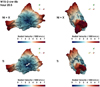 |
Fig. 1 Isosurfaces of mass fractions of |

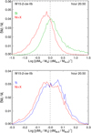 |
Fig. 2 Mass distribution of selected species versus the ratio |
![$R_{\textrm{i,Ni+X}}\,{=}\,\log [(\textrm{d}M_{\textrm{i}} / M_{\textrm{i}})(\textrm{d}M_{\textrm{Ni + X}} / M_{\textrm{Ni + X}})^{-1}]$](/articles/aa/full_html/2021/01/aa39335-20/aa39335-20-eq10.png)

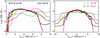 |
Fig. 3 Mass distributions of 1H, 4He, 12C, 16O, 28Si, 44Ti, and the quantity |
2.2 Modeling the evolution of the supernova remnant
Model W15-2-cw-IIb was used to initiate 3D MHD and HD simulations which describe the long-term evolution of the blast wave and ejecta, from the shock breakout to the interaction of the remnant with the wind of the progenitor star, covering ≈ 2000 yr of evolution. We adopted the numerical setup of the SNR model described in Orlando et al. (2019a, 2020). In particular, the evolution of the blast wave and ejecta were modeled by numerically solving the time-dependent MHD equations of mass, momentum, energy, and magnetic flux conservation in a 3D Cartesian coordinate system (x, y, z) and assuming an ideal gas law, P = (γ − 1)ρϵ, where P is the pressure, γ = 5∕3 the adiabatic index, ρ the mass density and ϵ the specific internal energy. The effects of self-gravity were neglected during the remnant evolution (starting ≈ 20 h after the core-collapse), because the ejecta are in free expansion3. The simulations include all physical processes relevant to describe the interaction of the stellar debris with the CSM: the deviations from equilibrium of ionization and from electron-proton temperature equilibration; the effects of energy deposition from radioactive decay of 56Ni and 56Co; the effects of an ambient magnetic field.
The simulations of the expanding SNR were performed using PLUTO v4.3 (Mignone et al. 2007, 2012), a modular Godunov-type code intended mainly for astrophysical applications and high Mach number flows in multiple spatial dimensions. The code is designed to make efficient use of massively parallel computers using the message-passing interface (MPI) for interprocessor communications. We used the MHD or HD module available in PLUTO, configured to compute intercell fluxes with a two-shock Riemann solver: the linearized Roe Riemann solver based on characteristic decomposition of the Roe matrix in the case of HD simulations, and the Harten-Lax-van Leer discontinuities (HLLD) approximate Riemann solver in the case of MHD simulations. As for the time-marching algorithm, we adopted either the Runge-Kutta scheme at third order (RK3) or the characteristic tracing (ChrTr) scheme. The combination of a two-shock Riemann solver (either Roe or HLLD) with one of the algorithms used to advance the solution to the next time level (either RK3 or ChrTr) in a spatially unsplit fashion yields the corner-transport upwind method (Colella 1990; Mignone et al. 2005; Gardiner & Stone 2005), one of the most sophisticated (and least diffusive) algorithms available in PLUTO. A monotonized central difference flux limiter (MC LIM, the least diffusive limiter available in PLUTO) for the primitive variables is used to prevent spurious oscillations that would otherwise occur in the presence of strong shocks. In the case of MHD simulations, the solenoidal constraint of the magnetic field is controlled by adopting a hyperbolic/parabolic divergence cleaning technique (Dedner et al. 2002; Mignone et al. 2010).
The code was extended by additional computational modules to calculate the deviations from electron-proton temperature equilibration and from equilibrium of ionization, and the energy deposition from radioactive decay. The former are calculated by assuming an almost instantaneous heating of electrons at shock fronts up to kT = 0.3 keV by lower hybrid waves (see Ghavamian et al. 2007) and by implementing the effects of Coulomb collisions for the calculation of ion and electron temperatures in the post-shock plasma (see Orlando et al. 2015 for further details). The deviations from equilibrium of ionization of the most abundant ions are calculated through the maximum ionization age in each cell of the spatial domain (Orlando et al. 2015). The energy deposition from radioactive decay is implemented following the approach described in Ferrand et al. (2019) which is based on the general formalism of Jeffery (1999) and Nadyozhin (1994). In particular we considered the dominant decay chain in which 56Ni (half-life 6.077 days) decays in 56Co (half-life 77.27 days) and the latter decays in stable 56Fe.
The chemical evolution of the ejecta is followed by adopting a multiple fluids approach as in Orlando et al. (2016). The fluids correspond to the species calculated in model W15-2-cw-IIb and are initialized with the abundances in the output of the SN model. The continuity equations of the fluids are solved in addition to our set of MHD equations. The different fluids mix together during the remnant evolution and, in particular when the ejecta interact with the reverse shock that develops during the expansion of the remnant. The density of a specific element in a fluid cell at time t is calculated as ρi = ρCi, where Ci is the mass fraction of each element and the index “i” refers to the considered element. This allows mapping of the spatial distribution of heavy elements both inside and outside the reverse shock at different epochs during the evolution.
At the beginning of the SNR simulations, the ejecta are distributed within a sphere with radius ≈ 1014 cm. Observations suggest thatthe morphology and expansion rate of Cas A are both consistent with a blast wave still expanding through the wind of the progenitor star4. Thus, for the CSM, we assumed a spherically symmetric wind with gas density proportional to r−2 (where r is the radialdistance from the center of explosion). Following Orlando et al. (2016), we fixed the wind density nw = 0.8 cm−3 at rfs = 2.5 pc (a rough estimate of the current outer radius of the remnant, assuming a distance of ≈ 3.4 kpc), which is slightly smaller than the best-fit value inferred by X-ray observations of Cas A (nw = 0.9 ± 0.3 cm−3; Lee et al. 2014) but well within the range of values constrained. We note that the r−2 wind profile is appropriate to describe the past evolution of Cas A till the current epoch. However, at later times, the remnant will expand through an ambient medium of which we ignore the structure and density distribution. The r−2 wind profile seems unlikely to extend at radii much larger than the current radius of the remnant because, there, it predicts unrealistic low values of the wind density. Since we ignore the structure of the still unshocked CSM, we assumed a progressive flattening of the wind profile to a uniform density nc = 0.1 cm−3; in this way, our wind density profile was described as  .
.
We investigated the effects of energy deposition from radioactive decay and the effects of an ambient magnetic field by performing three long-term simulations with the above effects switched either on or off. The models are summarized in Table 1. The first is a pure HD simulation that does not include the effects of radioactive decay (model W15-2-cw-IIb-HD); this simulation allowed us to study how the pristine structures and large-scale asymmetries originating from the neutrino-driven SN explosion contribute to shaping the remnant morphology at different epochs. Then we evaluated the effects of heating due to radioactive decay of 56Ni and 56Co by performing a HD simulation with these effects included (model W15-2-cw-IIb-HD+dec). Finally, we performed a MHD simulation (that also accounts for radioactive decay heating) to investigate the effects of an ambient magnetic field on the evolution of ejecta clumps and on the development of HD instabilities (responsible for the clump fragmentation) as the reverse shock interacts with the ejecta (model W15-2-cw-IIb-MHD+dec). Previous studies have shown that the magnetic field can envelope theexpanding clumps of ejecta, thus limiting the growth of HD instabilities because of the continuous increase of the magnetic pressure and field tension at the clump border (e.g., Orlando et al. 2012). As a consequence, the clumps can survive for a longer time.
In model W15-2-cw-IIb-MHD+dec, we assumed that the magnetic field is the relic of the field of the progenitor star. In this case, the simplest field configuration resulting from the rotation of the star and from the expanding stellar wind is a spiral-shaped magnetic field known as “Parker spiral” (Parker 1958). In our case, we considered a pre-SN magnetic field characterized by an average strength at the stellar surface5 B0 ≈ 500 G, which is a value well within the range observed for magnetic massive stars (mean surface field intensities inferred from Zeeman splitting in the range from about 2 to 30 kG; Donati & Landstreet 2009). We note that the simulations of the progenitor star as well as that of the SN explosion adopted here did not consider any magnetic field. So, following Orlando et al. (2019a), we described the magnetic field in the initial remnant interior to be the same as in the medium outside the progenitor star (namely the “Parker spiral”). Although this is a crude approximation6, the magnetic field is expected to play a role only locally in preserving clumps of ejecta from complete fragmentation after interaction with the reverse shock and not to influence the overall expansion and evolution of the remnant, which is characterized by a high plasma β (defined as the ratio of thermal pressure to magnetic pressure). Thus, for our purposes (namely to investigate the effects of the magnetic field in determining the structure of the mixing region between the forward and reverse shock), it was enough to introduce the Parker spiral in our MHD simulation.
Our mesh configuration is that described in Orlando et al. (2019a, 2020) which allows us to follow the large physical scales spanned during the remnant expansion. The initial computational domain is a Cartesian box that extends between − 1.2 × 1014 cm and 1.2 × 1014 cm in all directions, thus including the spatial domain of the output of model W15-2-cw-IIb. The box is covered by a uniform grid of 10243 zones, leading to a spatial resolution of ≈2.3 × 1011 cm. The center of explosion in model W15-2-cw-IIb is assumed to sit at the origin of the 3D Cartesian coordinate system (x0, y0, z0) = (0, 0, 0). During the evolution, the computational domain was gradually extended following the expansion of the remnant through the CSM and the physical quantities were remapped in the new domains. The domain is extended by a factor of 1.2 in all directions when the forward shock reaches one of the boundaries of the Cartesian box. The number of mesh points is kept the same at each remapping, so that the spatial resolution gradually decreases following the remnant expansion. All the physical quantities in the extended region are set to the values of the pre-SN CSM. In previous works, we estimated the errors on conservation of mass, momentum and energy introduced during the successive remapping to larger and larger grids; this approach did not introduce errors larger than 0.1% after 40 remaps (Ono et al. 2013; Orlando et al. 2019a). In the present case, we found that 69 remappings were necessary to follow the interaction of the blast wave with the CSM during 2000 yr of evolution and we found that the errors introduced are not larger than 1% (with the largest errors in the conservation of momentum). The final domain extends between − 9.4 pc and 9.4 pc in all directions, with a spatial resolution of ≈0.018 pc. All physical quantities were fixed to the values of the pre-SN CSM at all boundaries.
Setup for the simulated models.
3 Results
3.1 The remnant expansion through the stellar wind
The ejecta distribution soon after the shock breakout is already characterized by large-scale asymmetries (see Fig. 1). These reflect anisotropies of the 3D SN explosion developed stochastically7 mainly by convective overturn in the neutrino-heating layer and by the standing accretion shock instability (SASI; Wongwathanarat et al. 2017).
After the shock breakout, the interaction of the ejecta with the wind of the progenitor star drives a reverse shock that moves backwards through the ejecta. During the early phases of propagation of the blast wave through the wind, the metal-rich ejecta expand almost homologously, thus carrying the fingerprints of the asymmetric explosion. However, about 30 yr after the SN, when almost all 56Ni and 56Co have already decayed in stable 56Fe, the Fe-group elements start to interact with the reverse shock. The deceleration of the swept-up ejecta passing through the reverse shock leads to the development of HD instabilities (RT, Richtmyer-Meshkov, and KH shear instability; Gull 1973; Fryxell et al. 1991; Chevalier et al. 1992), which fragment the dominant high-entropy plumes of Fe- and Ti-rich ejecta into numerous small fingers. The RT growth is triggered by a crossing of the density and pressure gradients in the shocked ejecta: ∂P∕∂r > 0 and ∂ρ∕∂r < 0. This determines a large-scale spatial mixing of metal-rich ejecta (see Sect. 3.2).
Figure 4 compares the angle-averaged radii of the forward and reverse shocks resulting from our models at the age of ≈ 350 yr with those currently observed in Cas A (Gotthelf et al. 2001; Helder & Vink 2008). All SNR models are able to reproduce the observations within the error bars, although they slightly underestimate both shock radii. This is not surprising because the explosion energy of model W15-2-cw-IIb (Eexp = 1.5 B; see Table 1) is smaller than the value inferred from the observations, Eexp ≈ 2 B (e.g., Laming & Hwang 2003; Hwang & Laming 2003; Sato et al. 2020), although the ejecta mass of our models (Mej = 3.3 M⊙; see Table 1) is within the range of values discussed in the literature, Mej = [2−4] M⊙ (e.g., Laming & Hwang 2003; Hwang & Laming 2003; Young et al. 2006). A slightly higher explosion energy for the same ejecta mass would increase the radii for forward and reverse shock at the present age of the remnant. Once again we note that the SN model adopted here (W15-2-cw-IIb) was not tuned to describe the SN that produced the SNR Cas A, but was selected because it roughly reproduces post-explosion anisotropies which resemble the structure of Cas A (Wongwathanarat et al. 2017). So, the fact that the SNR models roughly reproduce the forward and reverse shock radii at the age of Cas A encourages us to consider the adopted SN model appropriate for a comparison with Cas A.
Figure 4 also shows that the models including the radioactive decay have results in slightly larger radii of the reverse and forward shocks than in model W15-2-cw-IIb-HD. In fact the energy deposition due to radioactive decay provides an additional pressure to the plasma which inflates instability-driven structures that possess a high mass fraction of decaying elements against their surroundings, thus powering the expansion of the ejecta (Gabler et al. 2020). As for the ambient magnetic field, as expected, it does not influence the overall expansion and evolution of the blast wave, which is characterized by a high plasma β: the evolution of reverse and forward shock radii is basically the same in models W15-2-cw-IIb-HD+dec and W15-2-cw-IIb-MHD+dec. Nevertheless, we expect that the magnetic field plays a role in preserving inhomogeneous structures (clumps) of ejecta from complete fragmentation by limiting the growth of HD instabilities at their borders (e.g., Orlando et al. 2008, 2012).
The effects of radioactive decay on the ejecta dynamics are also visible in the amount of Fe, Ti and Si that is heated by the reverse shock. Figure 5 shows the fraction of shocked masses of these elements versus time. When the heating deposition by radioactive decay is not included in the calculation (model W15-2-cw-IIb-HD), the shocked masses are systematically lower than the corresponding shocked masses when the heating deposition is included (models W15-2-cw-IIb-HD+dec and W15-2-cw-IIb-MHD+dec). At the age of Cas A, the models predict that ≈ 28−32% of Ti and ≈ 30−34% of Fe are shocked. Considering the tracer-particle-based post-processing with the large nuclear network, Wongwathanarat et al. (2017) estimated for model W15-2-cw-IIb a mass of 1.57 × 10⁻⁴ M⊙ of 44Ti and 9.57 × 10⁻² M⊙ of 56Ni. The initial mass of Ti is consistent with the analysis of NuSTAR observations, which suggests a total initial mass of 44Ti of 1.54 ± 0.21 × 10⁻⁴ M⊙ (Grefenstette et al. 2017). Thus, at the age of Cas A, the amount of shocked Ti (not considering its decay in 44Ca) and Fe is in the ranges [4.4−5.0] × 10−5 M⊙ and [2.9−3.3] × 10−2 M⊙, respectively. Some words of caution are needed here. In the present paper, we considered only 56Fe from 56Ni decay. However, there is additional Fe (other isotopes, e.g., 52Fe), which increase the total mass by some 10% (see Wongwathanarat et al. 2017, footnote 9). All our estimates of Fe mass should be considered as a lower limit to the total Fe mass. As for the 44Ti, for an e-folding time of 90 yr (the half-life of 44Ti is 63 yr), its mass at the age of Cas A (350 yr) would be in the range [0.94−1.1] × 10−6 M⊙.
Finally, we estimated the fraction of shocked Ti and Fe if the model had an explosion energy of Eexp ≈ 2 B, as inferred from observations (e.g., Laming & Hwang 2003; Hwang & Laming 2003; Sato et al. 2020). In this case, the ratio Eexp∕Mej would have been ≈ 0.6 B∕M⊙ (whereas, in our simulations, Eexp∕Mej ≈ 0.45 B∕M⊙) and the average velocity of the ejecta soon after the shock breakout (approximately given by  ) would have been a factor 1.15 higher than in our simulations. The slightly higher velocities with Eexp = 2 B would have advanced the interaction with the reverse shock, thus leading to a fraction of shocked Ti8 and Fe at the age of Cas A in the ranges [5.0−5.6] × 10−5 M⊙ (≈ 32−36%) and [3.2−3.6] × 10−2 M⊙ (≈ 34−38%), respectively.
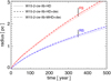 |
Fig. 4 Angle-averaged radii of the forward (red lines) and reverse (blue lines) shocks versus time for the three models investigated. The black crosses show the corresponding observational values at the current age of Cas A (Gotthelf et al. 2001); the vertical lines of the crosses show the observational uncertainty. |
3.2 Massdistribution in velocity space
HD instabilities that develop during the interaction of the ejecta with the reverse shock determine the structure and mixing of shock-heated ejecta in the region between the reverse and the forward shocks. Apart from the asymmetries already present in the ejecta at the shock breakout (see Fig. 1), the velocity distributions of elements at the various SNR ages also reflect the mixing between layers of different chemical composition, driven by the interaction of the ejecta with the reverse shock. Figure 6 shows the mass distributions of selected elements versus the radial velocity, vrad (left panels), and the LoS velocity, vLoS (right panels), for model W15-2-cw-IIb-HD+dec. The other two models (either without the radioactive decay, W15-2-cw-IIb-HD, or including the effects of an ambient magnetic field, W15-2-cw-IIb-MHD+dec) produce similar results and are presented in Appendix A. As in Fig. 3, vLoS is derived assuming the Earth vantage point lying on the negative y-axis and the remnant oriented as in the left panels in Fig. 1. Figure 6 reports 56Fe instead of [Ni + X] (as in Fig. 3) because almost all 56Ni and 56Co already decayed in 56Fe at the epochs considered.
The upper panels in Fig. 6 show the mass distribution of elements at the time when the reverse shock hits the Fe- and Ti-rich ejecta. By comparing these panels with Fig. 3, at this stage the reverse shock has already slowed down the expanding outer layers of the ejecta. The distributions of intermediate-mass and light elements at velocities larger than ≈ 8000 km s−1 have similarshapes with a slope much steeper than in the initial condition (soon after the shock breakout). This is a sign of efficient mixing in the region between the reverse and forward shocks. Nevertheless the initial order of the elements is roughly preserved, with light elements (H and He) residing at larger radii with higher velocities, and intermediate-mass elements (C, Si, O) at smaller radii with smaller velocities. At this time, the mass distributions of Fe and Ti are similar to those of the initial condition, suggesting an almost homologous expansion of these species before interaction with the reverse shock, although their broad maxima now extend up to ≈ 7500 km s−1 (≈ 7000 km s−1 in the initialcondition). This is mainly due to radioactive decay that powers the ejecta residing in regions of heating deposition (compare upper panels in Fig. 6 with upper panels in Fig. A.1). The mass distributions versus the LoS velocityshow large asymmetries in heavy and intermediate-mass elements, thus reflecting the large-scale asymmetries developed in the 3D SN explosion: Fe and Ti traveling toward (away from) the observer reach peak velocities up to ≈ 6000 km s−1 (≈ 7500 km s−1).
The middle panels in Fig. 6 show the mass distributions at the current age of Cas A. At this stage, the reverse shock has moved inward through the Fe- and Ti-rich plumes of the ejecta, heating a significant fraction of their masses (≈ 30% in model W15-2-cw-IIb-HD and ≈34% in models with radioactive decay included; see Fig. 5). The reverse shock has considerably slowed down the shocked ejecta and made the overall shapes of the high-velocity parts of the mass distributions of all elements more similar to each other. The broad maximum in the distributions now extends up to ≈ 5000 km s−1. The maxima and the positive slopes below the maxima are more or less the same as in the initial condition, thus indicating again that the unshocked ejecta continue to roughly expand homologously (although some effect due to radioactive decay is present in models W15-2-cw-IIb-HD+dec and W15-2-cw-IIb-MHD+dec; see Appendix A). The tails of the fastest ejecta above the distribution maxima are very similar to each other and characterized by steep slopes that stretch out the distributions up to ≈ 6000 km s−1, suggesting a considerable mixing between layers of different chemical composition driven by HD instabilities.
The mass distributions versus vLoS still show some asymmetries between red shifted and blue shifted profiles, although more reduced than at earlier times. The mass distributions of metal-rich ejecta extend in the velocity range − 4000 km s−1 < vLoS < 5500 km s−1 with the redshifted part more prominent than the blueshifted one, consistent with the fact the CCO approaches the observer. These results are in very nice agreement with the range of values inferred from observations of Cas A in the optical, infrared, and X-ray bands, which have revealed an overall velocity asymmetry of − 4000 to + 6000 km s−1 in the ejecta distribution (e.g., Lawrence et al. 1995; Reed et al. 1995; Willingale et al. 2002; DeLaney et al. 2010), and prominent redshifted LoS velocities of 1000−6000 km s−1 for Ti (Grefenstette et al. 2014, 2017).
The lower panels in Fig. 6 show the mass distributions at t ≈ 2000 yr, when most of Fe- and Ti-rich ejecta have been shocked (≈80%; see Fig. 5). Now the reverse shock has reached the deepest layers of the ejecta and the mass distributions significantly differ from those at the initial condition. The shapes of the distributions of all elements are very similar to each other due to very efficient mixing by HD instabilities. The maxima of the distributions versus vrad now extend between 1000 and 3000 km s−1 with peak velocities of 3500 km s−1. The asymmetries in the mass distributions versus vLoS are much more reduced with respect to previous epochs, but still showing a prominent redshift with LoS velocities up to 3000 km s−1 (2000−2500 km s−1 in the blueshifted part). In principle, the fingerprints of the asymmetric explosion might still be visible after 2000 yr of evolution. However, at this epoch, the remnant is likely to have interacted with an inhomogeneous ambient environment characterized by molecular or atomic clouds. In this case, its shape and the distribution of the ejecta might be largely influenced by this interaction, washing out the fingerprints of the explosion.
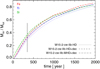 |
Fig. 5 Mass of shocked Si (green lines), Ti (blue), and Fe (red) normalized to their total mass versus time for the three SNR modelsanalyzed. The vertical black line marks the age of Cas A. |
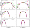 |
Fig. 6 Mass distributions of 1H, 4He, 12C, 16O, 28Si, 44Ti, and 56Fe versus radialvelocity, vrad (left panels), and velocity component along the LoS, vLoS (right panels) at the labeled times for model W15-2-cw-IIb-HD+dec. The upper panels correspond to the time when Fe and Ti start to interact with the reverse shock, the middle panels to the time corresponding to the age of Cas A, and the lower panels to t ≈ 2000 yr. |
3.3 44Ti and 56Fe distributions in the early phase of SNR evolution
The supersonic expansion of the ejecta through the wind environment leads to the development of an almost spherical forward shock and a more corrugated reverse shock due to propagation through ejecta inhomogeneities. As expected, HD instabilities (RT, Richtmyer-Meshkov, and KH shear instability; Gull 1973; Fryxell et al. 1991; Chevalier et al. 1992) develop and grow up at the contact discontinuity between shocked ejecta and shocked wind (see online Movie 1). The energy deposition due to the radioactive decay chain 56Ni → 56Co → 56Fe is effective during the first year of evolution. In this phase, regions rich in 56Ni and 56Co can be significantly heated to temperatures up to a few millions degrees.
As mentioned in Sect. 3.2, the reverse shock reaches regions of Fe- and Ti-rich ejecta about 30 yr after the SN event. The upper panels in Fig. 7 show the spatial distribution of Fe during this phase in model W15-2-cw-IIb-HD+dec. The other two models show similar distributions (see Appendix B). Assuming that the remnant is oriented in such a way that the Fe-rich fingers point toward the same direction as the extended Fe-rich regions observed in Cas A, the figure shows different viewing angles: with the perspective of the remnant in the plane of the sky (i.e., the vantage point is at Earth; left panel), with the perspective rotated by 90° about the z-axis (center panel), and with the perspective rotated by 180o about the z-axis (namely the vantage point is from behind Cas A; right panel). At this time, a significant fraction of intermediate-mass elements (asSi, O, and C) have already passed through the reverse shock (see upper panels in Fig. 6).
At the age of ≈30 yr, the Fe and Ti distributions are similar to those at the shock breakout, confirming that their evolution was almost homologous till the interaction with the reverse shock (see online Movie 1). The only significant change in their spatial distributions is due to heating by radioactive decay that inflated regions dominated by the decaying elements against their surroundings and provided an additional boost to the ejecta expansion (compare Fig. 7 with Fig. B.1). As a result, a dense shell forms at the interface between regions dominated by the decaying elements and the surrounding ejecta. During the evolution, the Ti has a spatial distribution very similar to that of Fe and the two species trace a similar 3D geometry. This is not surprising because, as discussed in Wongwathanarat et al. (2017), the two nuclei were basically synthesized in the same regions of (incomplete) Si burning and of processes like α-particle-rich freezeout (see also Nagataki et al. 1997; Magkotsios et al. 2010; Vance et al. 2020), and there is no physical process during their expansion able to decouple or decompose them.
As for the other species, after passing through the reverse shock, Fe and Ti become affected by HD instabilities which gradually grow as the species approach to the contact discontinuity. As discussed in detail in the literature, the growth conditions for such instabilities originate from the deceleration of the denser ejecta at their collision with the compressed but less dense shell of shocked CSM material, and they grow as long as a reverse shock moves backward into the slower ejecta (e.g., Chevalier et al. 1992; Jun & Norman 1996a; Wang & Chevalier 2001; Blondin & Ellison 2001). The development of HD instabilities is enhanced by the presence of shock deformation and pre-shock small- and large-scales perturbations of the ejecta (e.g., Orlando et al. 2012; Miceli et al. 2013; Tutone et al. 2020). These conditions are present in our case, in which the SN ejecta, before colliding with the reverse shock, are characterized by small-scale clumping and large-scale asymmetries that originated stochastically from the convective overturn in the neutrino-heating layer and SASI activity (e.g., Wongwathanarat et al. 2015, 2017).
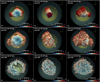 |
Fig. 7 Isosurfaces of the distribution of Fe at the time when the reverse shock starts to interact with the Fe- and Ti-rich plumes of ejecta (upper panels), at the age of Cas A (middle panels), and at t = 2000 yr (lower panels) for different viewing angles (from left to right) for model W15-2-cw-IIb-HD+dec. The opaque irregular isosurfaces correspond to a value of Fe density which is at 5% of the peak density; their colors give the radial velocity in units of 1000 km s−1 on the isosurface (the color coding is defined at the bottom of each panel). The semi-transparent clipped quasi-spherical surfaces indicate the forward (green) and reverse (yellow) shocks. The Earth vantage point lies on the negative y-axis. See online Movie 1foran animation of these data; a navigable 3D graphic of the Fe spatial distribution at the age of Cas A is available at https://skfb.ly/6TKRK. |
3.4 Structure of shocked ejecta at the age of Cas A
At the age of Cas A (middle panels in Fig. 7), about 2.45 M⊙ of ejecta were shocked. The HD instabilities are already well developed and have determined the progressive fragmentation of the initially large, metal-rich plumes of ejecta (rich in Fe and Ti) to smaller fingers of dense ejecta gas that protrude into the shocked wind material. The instabilities also enhance the mixing between layers of different chemical composition as evident from the middle panels in Fig. 6. At this age, large regions of shocked Fe-rich ejecta form in coincidence with the original large-scale fingers of Fe-group elements. There, several Fe- and Ti-rich shocked filamentary structures extend from the reverse toward the forward shock. As in Cas A, shocked Fe, Ti, and Si are arranged in a torus-like geometry, which is tilted approximately 30° with respect to the plane of the sky (see Fig. 8 and online Movie 2). This structure reflects the large-scale asymmetry of the Fe-group ejecta at the shock breakout, which mainly consist of three extended Fe-rich fingers. The latter define a plane in which metal-rich ejecta extend much more than perpendicularly to it. As a result, the ejecta lying close to this plane reach the reverse shock well before those in other directions, producing the observed torus-like structure. The plane is oriented with an ≈ − 30° rotation about the x-axis (the eastwest9 axis in the plane of the sky) and an ≈10° rotation about the z-axis (the northsouth axis in the plane of the sky). Interestingly, this orientation is very similar to that found by Orlando et al. (2016) for the plane in which the three Fe bullets lie that reproduce the observed distribution of shocked Fe and Si/S (namely ix ≈−30° and iz ≈ 25°, respectively).
The ejecta in the torus are dominated by morphological structures that resemble the cellular structure (appearing as rings on the surface of a sphere) of [Ar II], [Ne II], and Si XIII observed in Cas A (e.g., DeLaney et al. 2010; Milisavljevic & Fesen 2013). In some cases, the ring structures have RT fingers which extend outward, giving them the appearance of crowns as also observed in Cas A (e.g., Milisavljevic & Fesen 2013). Ring- and crown-like structures originate from a combined action of small-scale structures in the initial Fe-rich fingers and the development of HD instabilities after the passage of the reverse shock. In fact, soon after the breakout of the SN shock from the star, half of the mass of Ni-rich ejecta is concentrated in relatively small, highly enriched clumps and knots (see Fig. 10 in Wongwathanarat et al. 2017). Later on, this ejecta structure is kept in the distribution of Fe (the final product of Ni decay). A significant fraction of these small-scale clumps is located in the outermost tips of the largest Ni/Fe-rich fingers (see Fig. 10 in Wongwathanarat et al. 2017), so that they start to interact with the reverse shock at relatively early times (≈ 30 yr). The clumpy structure of the ejecta enhances the development of HD instabilities and leads to the formation of a filamentary pattern of shocked ejecta with ring-like features (e.g., Orlando et al. 2012, 2016).
The comparison between models W15-2-cw-IIb-HD and W15-2-cw-IIb-HD+dec shows that the radioactive decay affects the structure of shocked ejecta by further boosting Fe and Ti. Figure 9 shows radial profiles of Fe, Ti, and Si averaged over a solid angle of 30° in the direction of the east Fe-rich finger (roughly along the negative x-axis for an observer on Earth) and of the negative z-axis (i.e., where no Fe-rich fingers are present) for our three models. We note that a forward shock radius of ≈ 2.5 pc is reached earlier in models W15-2-cw-IIb-HD+dec and W15-2-cw-IIb-MHD+dec (≈ 360 yr) than in model W15-2-cw-IIb-HD (≈370 yr). The inflatedejecta produce a dense shell at the edge of regions with a high concentration of the decaying elements, which becomes evident at the age ≈30 yr as bumps in the radial profiles of Fe, Ti, and Si immediately before the reverse shock (see upper panels in Fig. 9; see also discussion in Sect. 3.3). Indeed, in models including the decay heating, the density at the outermost tip of the Fe-rich plumes is about a factor of ≈ 7 higher than in model W15-2-cw-IIb-HD (compare the red profiles at r∕Rfs = 0.6, in the upperpanels in Fig. 9), thus increasing the density contrast of the Fe-rich clumps with respect to the surrounding ejecta. As the Fe-rich plumes hit the reverse shock, the inflated dense ejecta in models W15-2-cw-IIb-HD+dec and W15-2-cw-IIb-MHD+dec penetrate more efficiently in the mixing region, leading to a more effective development of the ring- and crown-like structures (compare the middle panels in Fig. 9 at the age of Cas A, and Fig. 8 with Fig. B.2).
We note that the Fe-rich regions are circled by rings of Si-rich ejecta, another striking resemblance with the Cas A structure. This is evident in Fig. 8 (see also online Movie 2) where it is possible to clearly identify an almost complete ring of Si-rich ejecta around the northwest Fe-rich region (lower right panel), and an incomplete ring around the east region (upper right panel). These rings reflect the structure of the ejecta at the shock breakout and the dynamics during the subsequent remnant evolution. This can be seen from Fig. 9 showing that, before the Fe-rich finger starts to interact with the reverse shock (upper panels), the radial distribution of post-shock Si is almost the same along the two directions analyzed. In fact, in this early phase, the distribution of shocked Si is almost spherical. Fe-rich layers (also rich in Si) are enveloped by a Si-rich layer of the ejecta (compare red and green lines in the figure). As a result, as soon as Fe-rich fingers interact with the reverse shock, the Si density strongly increases in shocked ejecta located in the immediate surroundings of regions of shocked Fe. This is clearly evident in Fig. 10 that shows, for the three Fe fingers (pointing roughly to the east, to the west and to the north), the profiles of Fe, Ti and Si as a function of the distance from the center of the Fe fingers; the profiles are averaged over all directions in a plane tangential to the sphere at r ≈ 0.7 Rfs (immediately above the reverse shock). In all the models, a shell rich in Si envelopes each Fe-rich region.
Our models also predict that the initial large-scale asymmetries resulting from the SN explosion produce a spatial inversion of ejecta layersat the age of Cas A, leading locally to Fe-rich ejecta placed at a greater radius than Si-rich ejecta. This featureforms as a result of the high velocity and dense Fe-rich plumes of ejecta in a way similar to that described inOrlando et al. (2016) for Fe-rich pistons. Our models show that, soon after the shock breakout, the large-scale Fe-rich fingers have already protruded through the chemically distinct layers above and are enveloped by a less dense Si-rich layer. After the interaction with the reverse shock, the dense Fe-rich fingers push out the less dense material above (including Si), breaking through some of it, and leading to the spatial inversion of the ejecta layers. This is evident from the middle panels in Fig. 9 by comparing the average radial distribution of Fe along the east Fe-rich finger (red solid line) with the distribution of Si along the negative z-axis (where no Fe-rich fingers are present; dashed green lines). The inversion of the ejecta layers is much more evident in models including the radioactive decay, which contributes boosting the Fe-rich fingers out (see also Gabler et al. 2020). In these cases, the shocked Fe is denser than in model W15-2-cw-IIb-HD and, already at the age of Cas A, it extends to a greater radius than Si-rich ejecta outside Fe-rich fingers (compare red solid with green dashed lines), whereas in model W15-2-cw-IIb-HD the inversion is evident only at later times (see lower panels in Fig. 9). The inversion also causes the material of the outer layers (in particular Si) to be swept out by the Fe-rich fingers and to accumulate to the side of the shocked Fe regions (see Fig. 10).
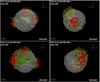 |
Fig. 8 Isosurfaces of the distributions of shocked Fe (red) and Si (green) at the age of Cas A for different viewing angles for model W15-2-cw-IIb-HD+dec. The upper left panel corresponds to the vantage point at Earth for Cas A. The opaque irregular isosurfaces correspond to a value of Fe and Si density which is at 25% of the respective peak density. The semi-transparent white surface indicates the reverse shock. See online Movie 2 for an animation of these data; a navigable 3D graphic of these distributions which includes also unshocked Fe and Si is available at https://skfb.ly/6UJYu. |
3.5 Structure of unshocked ejecta at the age of Cas A
The 3D spatial distributions of unshocked Fe and Si at the age of Cas A for model W15-2-cw-IIb-HD+dec are displayed in Fig. 11. An animation shows the 3D distributions rotating about the northsouth axis (Movie 2). At this epoch, the mass of unshocked ejecta from the models is ≈0.85 M⊙ which is in the range of values inferred from observations, namely between < 0.4 M⊙ (Hwang & Laming 2012; DeLaney et al. 2014)and ≈3 M⊙ (Arias et al. 2018), and in excellent agreement with recent findings inferred from infrared observations ( ; Laming & Temim 2020). This wide range of values inferred from observations is basically due to several sources of uncertainties, including the temperature and the clumpy structure of the unshocked ejecta (see also Raymond et al. 2018; Koo et al. 2018).
Our models show that the unshocked ejecta are highly structured. The amount of unshocked 56Fe is ≈ 0.062 M⊙; additional mass of Fe (≈10%; Wongwathanarat et al. 2017) comes from other Fe-group species, leading to a total of ≈ 0.068 M⊙ of unshocked Fe. This estimate is consistent with the ≈0.07 M⊙ of Fe that may be present in diffuse gas in the inner ejecta, as suggested by Laming & Temim (2020). About 50% of the unshocked Fe and Si are distributed in an irregular shell located in the proximity of the reverse shock (see upper row in Fig. 11). The two distributions are characterized by two large cavities (evident in the central columns of Fig. 11) corresponding to the directions of propagation of the large-scale Fe-rich plumes of ejecta (the initial asymmetry). In fact, the regions of shocked Fe in the mixing region are located exactly above these cavities (compare Figs. 8 and 11 and see Movie 2). Since the cavities are present in all simulations either including or not the Ni decay, we conclude that they form mainly because of the fast expansion of Fe in the directions of the large-scale plumes. The initial asymmetry in the SN explosion is mainly responsible for the largest cavities in our simulations. On the other hand, we note that the cavities are more extended in models including the Ni decay, thus reflecting the inflation of the Fe-rich regions driven by the radioactive decay heating of the initial Ni. This effect enhances the formation of the large-scale Si-rich rings visible in the shocked ejecta and encircling the Fe-rich regions. As a result, these rings are physically connected with the large cavities, a characteristic feature also present in the ejecta morphology of Cas A (e.g., Milisavljevic & Fesen 2015). This is particularly evident for the northwest Fe-rich region (compare Figs. 8 and 11; see online Movie 2).
The overall structure of the unshocked Si is similar to that found by Orlando et al. (2016), who considered parameterized initial post-explosion anisotropies in the ejecta, and it very closely resembles the bubble-like morphology of the Cas A interior (Milisavljevic & Fesen 2015). The analysis of near-infrared spectra of Cas A, including the [S III] 906.9 and 953.1 nm lines, shows a distribution of unshocked sulfur being very structured in the remnant interior (Milisavljevic & Fesen 2015), at odds with the results of Orlando et al. (2016), but in nice agreement with the Si distribution of our simulations. This is basically due to the fact that the SN model in Orlando et al. (2016) was one-dimensional, thus missing the mixing processes between different chemically inhomogeneous layers of the ejecta. In our simulations, the morphology of unshocked Fe and Si is enriched by several smaller-scale cavities that, especially in the case of Si, extend toward the remnant interior. Silicon was present in the Si shell of the progenitor and some of it formed from explosive oxygen burning behind the outgoing shock. Naturally, some of it was left in the remnant interior and some of it was mixed outward by the radial instabilities. Fe, Ti and Si were formed in neighboring regions, and all of them were affected by the same mixing processes, starting with the convective overturn triggered by neutrino heating, during the first second of the explosion, and followed by subsequent RT instability as the SN shock crosses the composition shell interfaces of the progenitor. These detailed dynamical effects during the early supernova stages were missing in the simulations of Orlando et al. (2016).
Another characteristic feature of the modeled ejecta structure which strikingly resembles that inferred from Cas A is the evidence of a “thick-disk” geometry for ejecta rich in Si, Ti, and Fe and which is tilted by an angle of ≈ −30° with respect to the plane of the sky (e.g., DeLaney et al. 2010; Grefenstette et al. 2017). This slanted thick-disk originates from the initial large-scale explosion asymmetry (see also Wongwathanarat et al. 2017 and Fig. 11 there) and, in fact, is oriented as the plane in which the three dominant high-entropy plumes lie at the time of shock breakout10. The thick-disk appearance is due to the fast expansion of the three plumes which makes the Si-, Ti-, and Fe-rich ejecta expanded more parallel to this plane than perpendicular to it.
The structure of the unshocked ejecta can be significantly affected by the radioactive decay of 56Ni and 56Co during the first year of the evolution (see also Gabler et al. 2020). Figure 12 shows the distributions of Fe and Ti at the age of Cas A for models W15-2-cw-IIb-HD and W15-2-cw-IIb-HD+dec (see also Movie 3). The distributions of Fe and Ti are very similar to each other in model W15-2-cw-IIb-HD, although there are some regions with dominant concentration of Fe and other with dominant concentration of Ti; in the presence of decay heating the differences are much more evident (see model W15-2-cw-IIb-HD+dec).
The distributions of unshocked Fe and Ti (especially in model W15-2-cw-IIb-HD) have properties similar to those witnessed after the shock breakout. In fact, they result from an almost homologous expansion of the ejecta. The innermost, still unshocked, Fe- and Ti-rich ejecta are more diluted than the outer shocked ones, consistent with the distributions of Ni and Ti obtained soon after the shock breakout (see Fig. 10 in Wongwathanarat et al. 2017). This is also consistent with the fact that the unshocked ejecta expanded homologously, whereas the shocked ejecta were strongly compressed by the reverse shock. A mass fraction of about 50% of unshocked Fe and Ti is enclosed in highly enriched clumps (second column in Fig. 12), which roughly form an irregular shell enclosing regions of more diluted Fe and Ti (in Fig. 12 compare thedifferent isosurfaces enclosing 30, 50, 75, and 95% of the total unshocked ejecta mass of the respective element).
When the effects of radioactive decay of 56Ni and 56Co are taken into account, soon after the shock breakout the heating by the energy release inflates the ejecta in regions with a high concentration of the decaying elements, pushing them against their surroundings (see also Gabler et al. 2020). As a result, the ejecta in these regions expand faster than in regions with a low concentration of Ni and Co. As in model W15-2-cw-IIb-HD, at the age of Cas A, the bulk of unshocked Fe (the decay product of Co) is enclosed in enriched clumps of ejecta forming an irregular shell. However, in model W15-2-cw-IIb-HD+dec, the shell is more developed and expanded (inflated) than in W15-2-cw-IIb-HD due to the additional pressure provided by the decay heating: about 75% of the total ejecta mass of unshocked Fe is concentrated in the shell (see 3rd column in Fig. 12 for model W15-2-cw-IIb-HD+dec; see also Movie 3). The tilted thick-disk appearance of Fe- and Ti-rich ejecta is slightly less evident if decay heating is effective. Regions with a high concentration of Ti (and a low concentration of Fe) do not expand as fast as Fe-rich regions and, in fact, a significant fraction of Ti is distributed in the innermost part of the remnant (see 3rd column in Fig. 12 for model W15-2-cw-IIb-HD+dec). With decay heating, the unshocked ejecta become more structured with sharper contours, and Ti-enriched regions appear more clearly offset from volumes with high Fe abundance. Without decay heating the Fe and Ti structures seem to be more interwoven (see model W15-2-cw-IIb-HD in Fig. 12).
We note that our models do not contain any mechanisms able to decouple Fe from Ti. Figure 13 shows the mass distributions of Si, Ti, and Fe versus the abundance ratio, Ri,Fe (where i stands for Si or Ti; see Sect. 2.1), at the age of Cas A for our three models. Negative values of Ri,Fe indicate relatively higher concentrations of Fe, and vice versa. The mass distributions of the selected elements versus Ri,Fe do not change significantly during the whole remnant evolution, thus indicating that the relative abundances of these elements in each computational cell do not change appreciably during the interaction of the ejecta with the reverse shock or because of the effects of Ni decay. This is plausible because neither of these effects can segregate the nuclear species on macroscopic scales. In fact the mass distributions obtained with the models including the Ni decay (models W15-2-cw-IIb-HD+dec, W15-2-cw-IIb-MHD+dec) are almost the same as those of the model neglecting the Ni decay (model W15-2-cw-IIb-HD).
The distributions of Ti and Fe versus RTi,Fe are similar to each other and have almost the same narrow and symmetric shape observed for Ti and [Ni + X] soon after the shock breakout (compare lower panels in Figs. 2 and 13). This result confirms that, at the age of Cas A, the bulk of Ti and Fe almost coexists in the mass-filled volume. This is not surprising because 44Ti and 56Ni were both synthesized in regions of Si burning and of processes like α-particle-rich freezeout and, after the shock breakout, the 56Ni decayed in 56Co and the latter in 56Fe. The spread of values in the range − 0.3 < RTi,Fe < 0.3 reflects some local differences of the abundance ratios of these species with clumps of ejecta which are with a higher concentration of either Ti or Fe. The mass distributions of shocked (dashed lines in Fig. 13) and unshocked (dotted lines) ejecta indicate that the former have a higher concentration of Fe (distributions peaking at negative values of RTi,Fe), whereas the latter have a higher concentration of Ti (distributions peaking at positive values). For instance, in model W15-2-cw-IIb-HD+dec, about 35% of Fe against 33% of Ti are shocked at the age of Cas A. Nevertheless, our models predict that a significant amount of Ti has already interacted with the reverse shock at this time. This is basically due to the fact that the outermost tip of the Fe- and Ti-rich plumes (the first to interact with the reverse shock) have a higher concentration of Fe than Ti, but carry also considerable amounts of Ti.
In the case of Si and Fe, the mass distributions are broad and asymmetric like those derived soon after the shock breakout (compare upper panels in Figs. 2 and 13), thus reflecting large differences in the abundance ratios of these two species. At the age of Cas A, however, the distributions of Si and Fe versus RSi,Fe appear sharper than those derived soon after the shock breakout, suggesting a significant mixing between the two species during the interaction with the reverse shock. As found for Ti, the mass distributions of shocked and unshocked ejecta suggest that the former have, on average, a higher concentration of Fe, whereas the latter have a higher concentration of Si. This reflects the spatial inversion of ejecta layers discussed in Sect. 3.4: Fe seems to be more concentrated at larger radii than Si, opposite to how they are formed before and during the explosion.
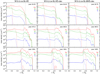 |
Fig. 9 Radial profiles of Fe (red), Ti (blue), and Si (green) averaged over a solid angle of 30° in the direction of the east Fe-rich finger (roughly along the negative x-axis in the left panels of Fig. 7; solid lines) and of the negative z-axis (i.e., where no Fe-rich finger is present; dashed lines) for our three models, at three different epochs. The vertical dotted line in each panel marks the average position of the reverse shock. The density of Ti was calculated by considering the tracer-particle-based post-processing with a large nuclear network (Wongwathanarat et al. 2017), but not considering its decay in 44Ca (for an e-folding time of 90 yr, the Ti density is scaled by a factor of 0.027). |
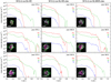 |
Fig. 10 Profiles of Fe (red), Ti (blue), and Si (green) as a function of the distance from the center of the Fe finger that roughly points to the east (top row), to the west (middle row) and to the north (botton row), at the age of Cas A, for our three models. The profiles are averaged over all directions in a plane tangential to the sphere at r ≈ 0.7 Rfs from the center of the explosion (namely immediately above the reverse shock). The density of Ti was calculated by considering the tracer-particle-based post-processing with a large nuclear network (Wongwathanarat et al. 2017), but not considering its decay in 44Ca (for an e-folding time of 90 yr, the Ti density is scaled by a factor of 0.027). The inset in the lower left corner of each panel shows a three-color composite image of the mass density distributions of Fe (red), Ti (blue), and Si (green) in the plane at r ≈ 0.7 Rfs. |
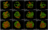 |
Fig. 11 Isosurfaces of the distributions of unshocked Fe (red) and Si (green) at the age of Cas A for different viewing angles (from left to right) for model W15-2-cw-IIb-HD+dec. The left panels correspond to the observer direction for Cas A. The isosurfaces enclose 50% (upper row), 75% (center row), and 95% (lower row) of the total mass of unshocked Fe and Si and correspond to a value of Fe (Si) density, in units of 10−26 g cm−3, which is 81 (25), 70 (16), and 55 (6.0), respectively. |
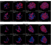 |
Fig. 12 Isosurfaces of the distributions of unshocked Fe (red) and Ti (blue) at the age of Cas A for different values of the mass fractions (decreasing from left to right; see the values reported at the end of the caption) and different viewing angles (front and side views) for models W15-2-cw-IIb-HD and W15-2-cw-IIb-HD+dec. The values of the mass fractions are selected so that the corresponding isosurfaces enclose, from left to right, 30, 50, 75, and 95% of the total mass of the respective unshocked species. The red isosurfaces correspond to a value of Fe density in model W15-2-cw-IIb-HD (W15-2-cw-IIb-HD+dec) which is, in units of 10−26 g cm−3, 119 (89), 95 (81), 71 (70), 40 (55), respectively; the blue isosurfaces correspond to a value ofTi density in model W15-2-cw-IIb-HD (W15-2-cw-IIb-HD+dec) which is, in units of 10−27 g cm−3 (considering the tracer-particle-based post-processing with a large nuclear network, Wongwathanarat et al. 2017, but not considering its decay in 44Ca), 2.1 (1.7), 1.7 (1.4), 1.2 (1.1), 0.7 (0.8), respectively (considering the decay of 44Ti in 44Ca, these values are scaled by a factor of 0.027, for an e-folding time of 90 yr). See online Movie 3 for an animation of these data; a navigable 3D graphic of these distributions is available at https://skfb.ly/6UMxI. |
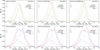 |
Fig. 13 Mass distribution of Si (green), Ti (blue), and Fe (red) versus the ratio |
![$R_{\textrm{i,Fe}}\,{=}\,\log [(\textrm{d}M_{\textrm{i}} / M_{\textrm{i}})(\textrm{d}M_{\textrm{Fe}} / M_{\textrm{Fe}})^{-1}]$](/articles/aa/full_html/2021/01/aa39335-20/aa39335-20-eq13.png)
3.6 44Ti and 56Fe distributions at the age of Cas A: comparison with NuSTAR observations
To further investigate the distribution of Ti versus Fe and to compare our model results with the findings from the analysis of NuSTAR observations (Grefenstette et al. 2014, 2017), we derived the distributions of shocked Ti and Fe (see Fig. 14) in addition to the distributions of unshocked Ti and Fe displayed in Fig. 12 (see also Sect. 3.5). In fact, present NuSTAR observations compared the observed distribution of Ti only with the distribution of the shocked Fe. Figure 14 shows that regions of shocked Fe are also rich in Ti. As expected, these regions are more extended in model W15-2-cw-IIb-HD+dec than in W15-2-cw-IIb-HD due to the inflation of the Fe-rich regions driven by the radioactive decay heating of the initial Ni. For the same reason, the small-scale RT fingers developing from the regions of shocked Fe and Ti are more developed in the presence of decay heating. We also note that 50% of the mass of the shocked Fe and Ti is enclosed in a few small clumps of the ejecta (see left panels in Fig. 14). These structures are the relic of the small-scale clumps present in the tips of the Fe-rich plumes of the ejecta soon after the shock breakout at the stellar surface (see Fig. 10 in Wongwathanarat et al. 2017).
Figure 15 shows the mass fraction ratio [CFe∕CTi] (upper 2 rows) and the logarithm of the abundance ratio, ![$\log [(\textrm{d}M_{\textrm{Fe}} / M_{\textrm{Fe}})\,{\times}\,(\textrm{d}M_{\textrm{Ti}} / M_{\textrm{Ti}})^{-1}]$](/articles/aa/full_html/2021/01/aa39335-20/aa39335-20-eq6.png) (lower 2 rows, see also online Movie 4), where dMFe and dMTi are the fractions of Fe and Ti in the domain cell. The mass fraction ratio can vary by 3 orders of magnitude in the 3D domain (in agreement with Vance et al. 2020; see also Nagataki et al. 1998). Assuming that the masses of Fe (total mass11 of 9.57 × 10⁻² M⊙) and Ti (total mass12 of 1.57 × 10⁻⁴ M⊙) are diluted in a similar mass-filled volume, we expect an average mass fraction ratio of ≈ 600. Figure 15 shows that the variations of the mass fraction ratio around this average value can be even larger than a factor of 10: regions with a ratio >600 (in yellow and red in the figure) have the highest concentration of Fe relative to Ti, whereas regions with ratio below ≈ 600 (in dark blue) have the lowest concentration of Fe with respect to Ti. The regions with dominant concentration of Fe (in red) and those with dominant concentration of Ti (in blue) are clearly evident in the 3D distribution of the abundance ratio (lower 2 rows of Fig. 15).
(lower 2 rows, see also online Movie 4), where dMFe and dMTi are the fractions of Fe and Ti in the domain cell. The mass fraction ratio can vary by 3 orders of magnitude in the 3D domain (in agreement with Vance et al. 2020; see also Nagataki et al. 1998). Assuming that the masses of Fe (total mass11 of 9.57 × 10⁻² M⊙) and Ti (total mass12 of 1.57 × 10⁻⁴ M⊙) are diluted in a similar mass-filled volume, we expect an average mass fraction ratio of ≈ 600. Figure 15 shows that the variations of the mass fraction ratio around this average value can be even larger than a factor of 10: regions with a ratio >600 (in yellow and red in the figure) have the highest concentration of Fe relative to Ti, whereas regions with ratio below ≈ 600 (in dark blue) have the lowest concentration of Fe with respect to Ti. The regions with dominant concentration of Fe (in red) and those with dominant concentration of Ti (in blue) are clearly evident in the 3D distribution of the abundance ratio (lower 2 rows of Fig. 15).
From Figs. 14 and 15, we conclude that our model is in line with the observation of (shocked) regions with high concentrations of Fe but low abundance of 44Ti as reported by Grefenstette et al. (2017) on grounds of NuSTAR results. In particular, these authors found Ti-rich ejecta located both exterior and interior to the reverse shock, as predicted in our simulations (see Figs. 12, 14, 15 and online Movie 4). As in Cas A, in our models the bulk of shock-heated Ti is located in regions of shock-heated Fe, but there are some regions of shock-heated Fe (marked yellow in the distribution of mass-fraction ratio and red in the distribution of abundance ratio; see shocked ejecta in Fig. 15) with a low concentration of Ti that can even be considerably lower than a factor of 2 (see upper panels in Fig. 15; see also Wongwathanarat et al. 2017). These variations of the mass-fraction ratio of Fe and Ti are the relic of the structure of the two nuclei when they were synthesized. This is also consistent with the evidence that, in general, the concentration of Fe in shocked ejecta is slightly higher than average (mass distributions of shocked ejecta peaking at negative values of RTi,Fe) in all our three models (see Fig. 13). Our models also predict that a significant amount of unshocked Fe is interior to the reverse shock, preferentially in regions with a relatively high concentration of Ti (RTi,Fe ≈ 0.05). However unshocked Fe cannot be detected in Cas A until it is heated by the reverse shock.
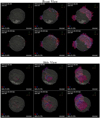 |
Fig. 14 Same as in Fig. 12, but for the distributions of shocked Fe (red) and Ti (blue). The values of the mass fractions are selected so that the corresponding isosurfaces enclose, from left to right, 50, 75, and 95% of the total mass of the respective shocked species. The red isosurfaces correspond to a value of Fe density in model W15-2-cw-IIb-HD (W15-2-cw-IIb-HD+dec) which is, in units of 10−25 g cm−3, 72 (50), 35 (26), 7.5 (7.9), respectively; the blue isosurfaces correspond to a value of Ti density in model W15-2-cw-IIb-HD (W15-2-cw-IIb-HD+dec) which is, in units of 10−26 g cm−3 (considering the tracer-particle-based post-processing with a large nuclear network, Wongwathanarat et al. 2017, but not considering its decay in 44Ca), 21 (15), 10 (7.9), 2.8 (2.5), respectively (considering the decay of 44Ti in 44Ca, these values are scaled by a factor of 0.027, for an e-folding time of 90 yr). A navigable 3D graphic of these distributions is available at https://skfb.ly/6UMxI. |
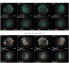 |
Fig. 15 3D distributions of mass fraction ratio [CFe∕CTi] (upper 2 rows) and log of abundance ratio, |
![$\log [(\textrm{d}M_{\textrm{Fe}} / M_{\textrm{Fe}})\,{\times}\,(\textrm{d}M_{\textrm{Ti}} / M_{\textrm{Ti}})^{-1}]$](/articles/aa/full_html/2021/01/aa39335-20/aa39335-20-eq14.png)
![$\log [(\textrm{d}M_{\textrm{Fe}} / M_{\textrm{Fe}})\,{\times}\,(\textrm{d}M_{\textrm{Ti}} / M_{\textrm{Ti}})^{-1}]$](/articles/aa/full_html/2021/01/aa39335-20/aa39335-20-eq15.png)
3.7 Properties of X-ray emitting ejecta at the age of Cas A
Cas A observations show X-rays by thermal emission arising from optically thin shocked plasma and by nuclear transitions of unstable elements (in particular 44Ti). In the first case, the contribution of the ith atomic species is proportional to the Emission Measure (EM), defined as EM = ∫ nenidV (where ne is the electron density, ni the density of species i, and dV the volume element); in the second case, the emission is proportional to the density of the unstable element. For a better comparison of the model results with X-ray observations of Cas A, Fig. 16 shows the EM of shocked Fe (red) and Si (green) integrated along the y-axis (i.e., the LoS assuming the vantage point at Earth) at the age of Cas A for our three models; the figure also shows the column density, nTi, of shocked and unshocked Ti (both contributing to X-ray emission; blue) at the same epoch. In Appendix C, we compare the EM distributions of shocked Fe and Ti integrated along the y-axis at the age of Cas A for our three models and the corresponding column density maps of unshocked Fe and Ti.
The resemblance of our models with the morphology of Cas A is impressive. Shocked Fe and Si are characterized by a highly inhomogeneous and filamentary structure with Fe-rich regions surrounded by Si-rich ejecta as observed in Cas A. These characteristics are more evident in models including the radioactive decay, because the Fe-rich ejecta penetrating the reverse shock are faster and denser (or, in other words, have a higher contrast of velocity and density with respect to the surrounding ejecta) than in model W15-2-cw-IIb-HD (see Sect. 3.4). Once more, this underlines the role played by the decay heating in shaping the final remnant morphology.
The fingers of shocked Fe are more evident (and well defined) in model W15-2-cw-IIb-MHD+dec than in the others. In this case, the magnetic field lines in the mixing region follow the plasma structures formed during the growth of HD instabilities at the contact discontinuity. This leads to the development of a preferentially radial component around the RT fingers (e.g., Mac Low et al. 1994; Jun & Norman 1996b). The tension of the field lines determines a more laminar flow around the fingers and limits the growth of HD instabilities which would destroy and fragment the Fe-rich structures (see also Fragile et al. 2005; Orlando et al. 2008, 2012). As a result, the fragmentation of the crown-like structures in the mixing region is less efficient and the structures survive for a longer time. The effect of magnetic field is also evident in Fig. 9, where the density structure of Fe, Ti, and Si is different when comparing models W15-2-cw-IIb-HD+dec and W15-2-cw-IIb-MHD+dec (see also Appendices A and B for the effects of an ambient magnetic field on the structure of the ejecta).
Figure 16 also shows the column density, nTi, of 44Ti at the age of Cas A, a proxy of the X-ray emission expected from nuclear transitions of unstable Ti. The bulk of this species is concentrated in the northern hemisphere, consistent with the initial asymmetry, suggesting that its momentum direction points to the north and is tilted by ≈30° out of the plane of the sky away from the observer. The momentum direction of Ti is roughly opposite to the direction of the CCO kick velocity pointing southward toward the observer (see also Wongwathanarat et al. 2017). This is in rough agreement with NuSTAR observations of Cas A that have shown an average momentum direction of Ti to the north, tilted by 58° ± 20° out of the plane of the sky away from the observer, opposite to the inferred direction of motion of the CCO (Grefenstette et al. 2017). The figure also shows that Ti-rich ejecta would emit from regions located both interior and exterior to the reverse shock, in agreement with the Ti distribution discussed in Sect. 3.6 and, again, with NuSTAR observations (Grefenstette et al. 2017). In the case of shocked ejecta, most of the emission from Ti would originate from regions with significant emission from shocked Fe (purple areas in Fig. 16), although there are also regions with prominent Fe emission and low contribution from shocked Ti (more reddish areas in Fig. 16).
The map of nTi in model W15-2-cw-IIb-HD is more clumpy than in the other two cases, suggesting that the distribution of Ti was smoothed by Ni radioactive heating occurring at early times in models W15-2-cw-IIb-HD+dec and W15-2-cw-IIb-MHD+dec. Interestingly, the NuSTAR images show a clumpy distribution of 44Ti which is remarkably similar to that produced by model W15-2-cw-IIb-HD. We note that, in models with decay heating, all of the decay energy is assumed to be deposited in the ejecta instead of allowing for some γ-ray leakage from the inner part of the remnant. Thus, these models most likely overestimate the smoothing effect by decay heating. In the light of this, the models W15-2-cw-IIb-HD and W15-2-cw-IIb-HD+dec represent the two extreme cases of either no or full energy deposition, and the case of Cas A should be between the two.
Figure 16 also shows that both the forward and reverse shocks deviate from a spherically symmetric expansion around the center of the explosion (compare solid and dashed contours in Fig. 16). They expand faster to the northwest than to the southeast. This is consistent with the initial large-scale asymmetry in which Ni and Ti were both mostly concentrated in the northern hemisphere propagating away from the observer, whereas the CCO travels in the southern hemisphere toward the observer with a kick velocity of ≈ 600 km s−1 (Wongwathanarat et al. 2010, 2013, 2017). We note that observations of Cas A in different bands also show that the forward and reverse shocks deviate from a spherically symmetric expansion; in particular, the reverse shock is offset to the northwest by ≈ 0.22 arcmin (≈ 0.2 pc at the distance of 3.4 kpc) from the geometric center of the forward shock (Gotthelf et al. 2001). However, at odds with the observations, in our simulations the geometric centers of the two shocks coincide and both are offset to the northwest by ≈ 0.13 pc from the center of the explosion.
Figure 17 displays the profiles of the forward and reverse shock velocities versus the position angle in the plane of thesky for model W15-2-cw-IIb-HD+dec at the age of Cas A (again, we found similar results for the other two models). These values can be compared with the forward and reverse shock velocities measured in the observer frame from the analysis of observations. The expansion of the forward shock shows velocities around ≈ 5500 km s−1 consistent with observations in different wavelength bands (e.g., DeLaney & Rudnick 2003; Patnaude & Fesen 2009; Fesen et al. 2019). As for the reverse shock, we found that our models predict an average expansion with velocities ranging between 2000 and 4000 km s−1. This is consistent with the velocities inferred in the eastern and northern hemisphere of the remnant (e.g., Sato et al. 2018; Fesen et al. 2019), but it is in clear contrast to the values inferred from observations in the western hemisphere, where the reverse shock appears to be stationary or even moving inward in the observer frame (see shaded area in Fig. 17; e.g., Helder & Vink 2008; Sato et al. 2018).
The origin of this asymmetry in the reverse shock properties is vividly debated in the literature. Our ejecta morphology and many other model features show great resemblance to Cas A. However, the fact that our simulations do not reproduce the displacement of the center of the reverse shock relative to the center of the forward shock points to something missing. Our simulations assume an isotropic wind; but the interaction of the forward shock with an anisotropic CSM might play a role. For instance, an initial spherically symmetric blast wave expanding through an ambient environment characterized by global anisotropy can produce an offset between the geomeric centers of the forward and reverse shocks (see, for instance, upper left panel in Fig. 2 in Orlando et al. 2007). So, our results seem to suggest that environmental asymmetries might play a role in displacing the center of the forward shock from the explosion center and probably also in shifting it relative to the center of the reverse shock (Orlando et al., in prep.).
From the models, we derived the distribution of the EM as a function of electron temperature, kTe, and ionization age, ne t (a measure of the deviations from equilibrium of ionization; see Sect. 2.2 and Orlando et al. 2016 for a description of how kTe and ne t are calculated), for the shocked plasma. These distributions are very useful for a quantitative comparison of the model results with X-ray observations. Figure 18 shows the distributions derived from model W15-2-cw-IIb-HD+dec at the age of Cas A. The distributions derived from the other two models give analogous results. The figure shows that the X-ray emitting plasma is largely out of equilibrium of ionization with the EM distribution peaking at kTe ≈ 2 keV and ne t ≈ 2 × 1011 cm−3 s. This result is similar to that found by Orlando et al. (2016) who designed a model with artificial ad-hoc initial conditions to reproduce the structure of Cas A. Indeed, our models (in which the initial large-scale asymmetry originates from stochastic anisotropies that developed through HD instabilities triggered by neutrino heating soon after core bounce) predict an EM distribution at the age of Cas A that is in excellent agreement with the results from the analysis of X-ray observations of Cas A (e.g., Hwang & Laming 2012; Lee et al. 2014; Greco et al. 2020). In particular, we found that the distributions of kTe and net derived from the models span ranges of values similar to those observed (the observed ranges are indicated by the white cross in Fig. 18), and they are highly peaked in agreement with the findings of Hwang & Laming (2012). As suggested by these authors, the peaked distributions reflect multiple secondary shocks following reverse shock interaction with ejecta inhomogeneities.
Figure 19 shows the average EM-weighted velocity of shocked Fe and Si along the LoS derived from model W15-2-cw-IIb-HD+dec (again the other two models yield similar results). As expected, the bulk of high-velocity shocked ejecta that are rich in Si and Fe is concentrated in regions where the large-scale metal-rich ejecta plumes interact with the reverse shock. The highest redshifted Si-rich ejecta (vLoS ≈ +5000 km s−1) form a large ring-like feature to the northwest; this is the result of the Fe-rich plume which breaks through theSi layer and determines a large Fe-rich region. The highest blueshifted Si-rich ejecta (vLoS ≈−5000 km s−1) are concentrated in the east region. These two features have the highest absolute values of the velocity along the LoS. The shocked Fe is also concentrated in the large redshifted region to the northwest and the blueshifted region to the east. The velocity pattern resembles the Doppler images derived from observations of Cas A (e.g., Willingale et al. 2002; DeLaney et al. 2010), and matches remarkably well the approximate velocity range inferred from observations (− 4000 < vLoS < +5000 km s−1).
It is worth to note that the model presented in Orlando et al. (2016) reproduces the distribution of the ejecta in Cas A in many details. In that case, the model adopted artificial initial conditions with the aim to identify a parameterized initial large-scale asymmetry and to constrain the masses and energies of the post-explosion anisotropies that are able to reproduce the observed distributions of Fe and Si/S. Conversely, in the models presented here, the initial large-scale asymmetry originates from the stochastic growth of anisotropies due to HD instabilities triggered by neutrino heating soon after core bounce. No fine-tuning was performed to match the morphology of Cas A. These models therefore demonstrate that the basic properties of the ejecta structure in Cas A can be naturally explained as originating from asymmetries arising from post-shock convective instability developing in the first second of the explosion. The observed features are the fingerprints of a neutrino-driven SN explosion. Nevertheless, our new simulations fail in reproducing another crucial aspect of the Cas A morphology, namely the formation of the two Si-rich wide-angle “jets” (also called Si-rich “sprays” in the literature). These features may result from post-explosion phenomena (as, for instance, disk accretion of fallback matter by the new-born neutron star; Chevalier 1989; Piro & Ott 2011) not considered in our simulations.
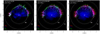 |
Fig. 16 Emission measure, EM, of shocked Fe (red) and Si (green) integrated along the y-axis (i.e., the LoS assuming the vantage point at Earth), and column density, nTi, of Ti (both shocked and unshocked; blue) at the age of Cas A for our three models. The solid contours mark cuts of the forward andreverse shocks in the plane of the sky passing through the center of the explosion; the dashed lines mark the same cuts but for spheres with the centers coincident with the center of explosion and radii corresponding to the average radii of the forward and reverse shocks. The two crosses in each panel mark the center of the explosion and the geometric center of the forward and reverse shocks offset to the northwest. |
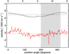 |
Fig. 17 Forward (black) and reverse (red) shock velocities versus the position angle in the plane of the sky for model W15-2-cw-IIb-HD+dec at the age of Cas A. The dashed horizontal lines mark the median values of the respective velocities. The shaded area marks the position angle where the reverse shock appears to be stationary or even moving inward in observations of Cas A (e.g., Helder & Vink 2008; Sato et al. 2018). |
 |
Fig. 18 Distribution of emission measure versus electron temperature (kTe) and ionization age (net) at the epoch of Cas A derived from model W15-2-cw-IIb-HD+dec compared with the results of Chandra X-ray observations. The large white cross marks the ranges of kTe and ne t derived from an X-ray survey of ejecta in Cas A (Hwang & Laming 2012); the small yellow crosses mark the values inferred from the analysis of regions dominated by thermal emission of shocked ambient gas (Lee et al. 2014). |
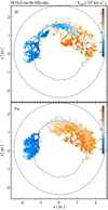 |
Fig. 19 Maps of average EM-weighted velocity along the LoS for shocked Si (upper panel) and Fe (lower panel) at the age of Cas A for model W15-2-cw-IIb-HD+dec. The approximate velocity range is ± 5000 km s−1 (see color bar on the right in units of 1000 km s−1). The solid contours mark the cuts of the forward and reverse shocks in the plane of the sky passing through the center of the explosion. These images correspond to the effective Doppler maps derived from observations. |
3.8 Distribution of ejecta at later times
At later times, the remnant expands further through the wind of the progenitor star. At the end of our simulations, at the age of ≈ 2000 yr, most of the metal-rich ejecta (≈80%) have been shocked (see Fig. 5). HD instabilities have led to well developed large-scale fingers and dominate the structuring and considerable mixing of shocked ejecta. The efficient mixing is evident from the high-velocity tails of the mass distributions of elements versus radial velocity that are very similar to each other (see lower right panel in Figs. 6, A.1, and A.2). The remnant interior is characterized by material with density much lower than that of the shock-heated ejecta due to the adiabatic expansion of the unshocked plasma and the high compression of shock-heated ejecta by the reverse shock; however, voids and cavities remain, even when the unshocked ejecta are very diluted. The spatial distribution of shocked Fe and Ti (or its decay product 44Ca) suggests that most of their masses are concentrated in the remnant hemisphere that propagates away from the observer, taking on the appearance of the spiny outer shell13 of a chestnut (see lower panels in Fig. 7). This is consistent with the initial large-scale asymmetry that launched most of Fe and Ti to the north, away from the observer and opposite to the CCO kick velocity (see Fig. 1 and Wongwathanarat et al. 2017).
Figure 20 shows the mass distributions of Si, Ti (or, most likely, its decay product 44Ca), and Fe versus the abundance ratio, Ri,Fe (where i stands for Si or Ti), at t ≈ 2000 yr for our three models. These distributions appear more peaked than those derived at previous times, although the changes are small. Again this indicates that, on average, the relative abundances of these elements in each computational cell do not change appreciably after the passage through the reverse shock. At this epoch, the distribution of Si versus RSi,Fe slightly differs among the three models, that is the distribution being more peaked in models including the radioactive decay (compare upper panels in Fig. 20). The distributions of Ti (44Ca) and Fe versus RTi,Fe are still similar to each other in the three models indicating that, after 2000 yr of evolution, the bulk of Ti (44Ca) and Fe almost coincides. As during previous epochs, the figure shows that, on average, shocked ejecta (dashed lines) have a higher concentration of Fe, whereas unshocked ejecta (dotted lines) have a higher concentration of Ti (44Ca), which is again a relic of the efficient outward mixing of highly Fe-enriched ejecta.
Our simulations at the age of ≈2000 yr can be compared with other O-rich SNRs that are more evolved than Cas A, although some word of caution is needed here: the progenitor model adopted for our study was a stripped star that had lost most of its H envelope, its He-core mass was specific to be in the ballpark of estimates for Cas A, and the explosion energy is also not generally valid for all SNe. Nevertheless, an interesting candidate for a comparison with our models is an older cousin of Cas A, the Galactic core-collapse SNR G292.0+1.8 (in the following G292), with an estimated age of ≈ 3000 yr (e.g., Ghavamian et al. 2005; Winkler et al. 2009; Gonzalez & Safi-Harb 2003) and average forward and reverse shock radii of ≈ 7.7 pc and ≈ 3.8 pc, respectively (at a distance of ≈6 kpc; Park et al. 2007; Gaensler & Wallace 2003; Bhalerao et al. 2015), similar to those derived at the end of our simulations (≈ 8.2 pc and ≈ 4.2 pc, respectively, at the age of≈2000 yr). The progenitor was most likely a star with a zero-age-main-sequence mass in the range between 13 and 30 M⊙ (Bhalerao et al. 2019). The total ejecta mass inferred from radio and X-ray observations is in the range of 6− 8 M⊙ (Gaensler & Wallace 2003; Bhalerao et al. 2015), whereas the estimated explosion energy is Eexp ≤ 1 B (Gonzalez & Safi-Harb 2003), although the latter value has large uncertainties. We note that the ejecta mass, Mej, in G292 is higher than in our model (and in Cas A) and the explosion energy, Eexp, is lower (see Table 1). This means that the ratio Eexp∕Mej ≈ 0.14 B∕M⊙ is considerably lower than in our simulations (Eexp∕Mej ≈ 0.45 B∕M⊙), thus suggesting an average velocity of the ejecta soon after the shock breakout at the stellar surface (approximately given by  ) of ≈ 3700 km s−1 versus the
  km s−1 of our models. So, we advise the reader to be cautious when comparing our models with G292. In particular, our models with their higher ejecta velocities should evolve on a shorter time scale than G292. Having said that, we note that, as Cas A (and as predicted by our models), G292 is characterized by a knotty and filamentary structure. At odds with our models, the morphology of G292 also shows evidence of an equatorial belt, probably originating from shocked dense circumstellar material (not modeled in our simulations), and thin circumferential filaments (e.g., Park et al. 2004, 2007).
For a better comparison between our models and G292, we rotated the system about the three axes to roughly match the orientation of the neutron star kick inferred for G292 and the observed remnant asymmetries, namely ix = −30°, iy = 60o, iz = −90° (see Fig. 21). The analysis of Chandra observations of G292 has revealed electron temperatures ranging, in general, between 0.5 and 2 keV, although there are isolated knots in the northwest hemisphere with significantly higher electron temperatures (up to kTe ≈ 4 keV; Bhalerao et al. 2019). The ionization time ranges, in general, between 3.4 × 1010 cm−3 s and 3 × 1012 cm−3 s, with few small regions in the northwest with values up to ne t ≈ 1013 cm−3 s. In Fig. 22 we compare the inferred ranges of values mentioned above with the distribution of the EM as a function of kTe and net at t ≈ 2000 yr for model W15-2-cw-IIb-HD+dec. At this stage of the evolution, the EM distribution is about an order of magnitude lower than that at the age of Cas A due to the remnant expansion that has diluted the X-ray emitting plasma. The ejecta at this epoch are on average characterized by lower temperatures and slightly higher ionization ages than found at the age of Cas A, in agreement with the adiabatic expansion of the remnant and with the progressive approach of the shocked plasma to ionization equilibrium. In particular, the bulk of the shocked ejecta mixed with shocked wind material extends over the ranges 0.6 keV < kTe < 2 keV and 1011 cm−3 s < net < 1012 cm−3 s, peaking at kTe ≈ 1 keV and ne t ≈ 3.5 × 1011 cm−3 s. These values are consistent with those inferred for G292, although the observed remnant shows higher values of ne t, indicating that the plasma is closer to the equilibrium of ionization. This could be a consequence of the fact that the ratio Eexp∕Mej of G292 is considerably lower than for our models or that the remnant is expanding through an ambient medium which is denser than that of our model. Nevertheless, we consider it as astounding that the modeled remnant describes the properties of the shocked plasma inferred from observations so closely, especially because our models have not been tuned to describe the progenitor star, the SN explosion, the CSM, and the evolution of G292.
The observations have also shown that the ejecta in G292 are characterized by high velocities, with the number of blueshifted knots larger than that of redshifted ones (Ghavamian et al. 2005; Bhalerao et al. 2015). The measurements of the radial velocities (i.e., the velocities along the LoS) reveal ranges between − 1800 km s−1 < vrad < 1490 km s−1 in the eastwest direction, and − 3570 km s−1 < vrad < 2340 km s−1 in the northsouth direction, thus indicating that the fastest ejecta are blueshifted and distributed along the northsouth direction (Ghavamian et al. 2005; Winkler et al. 2009). This evident asymmetry has been interpreted as the result of an asymmetric SN explosion, with the stellar debris ejected fastest along an axis oriented approximately north-south in the plane of the sky and in direction toward the observer (Winkler et al. 2009). The range of velocities inferred from observations is consistent with the range of radial velocities predicted by our models at the age of ≈ 2000 yr (see Fig. 6), with the high-velocity tails extending up to vrad ≈ 3500 km s−1.
The observed spatial distribution of the ejecta is highly inhomogeneous in G292, with different morphologies for intermediate-mass elements (as O, Ne, and Mg) on one hand, and for tracers of explosive nucleosynthesis (most notably Si, S, and Fe) on the other hand. In particular, O, Ne, and Mg are observed to be distributed within the whole remnant, whereas Si-rich ejecta are concentrated mainly in the northwest area (e.g., Park et al. 2002; Yang et al. 2014; Bhalerao et al. 2019). Recently, Fe-rich ejecta have been found concentrated in Si-rich regions to the northwest (Bhalerao et al. 2019). These properties of the ejecta distributions resemble those found in our models, with Si- and Fe-rich shocked ejecta concentrated in the northwest hemisphere where the high-entropy plumes from the SN explosion mainly interact with the reverse shock. Figure 23 shows the distributions of the EM of shocked Fe (red), Si (green), and intermediate-mass elements (O, Ne, and Mg; blue) integrated along the LoS for model W15-2-cw-IIb-HD+dec. The map assumes the orientation that roughly matches the direction of the neutron star kick inferred for G292; the LoS is along the y-axis (see Fig. 21). As expected, the model shows that most of the shocked Si and Fe are concentrated in the northwest hemisphere, whereas intermediate-mass elements are, on average, distributed over the whole remnant area. For asymmetric explosions with high neutron star kicks, Wongwathanarat et al. (2013) predicted such an asymmetry of the spatial distributions of elements including and heavier than Si, which are expected to be ejected predominantly in the hemisphere opposite to the kick direction of the neutron star. In contrast, lighter elements (C, O, Ne, Mg) were found to exhibit little or no (anti-)correlation with the neutron star kick.
The similarities between the ejecta structure in G292 and our simulations support the idea that the parent SN of the observed remnant was characterized by a large-scale asymmetry with characteristics analogous to those analyzed in our models. The direction of propagation of the neutron star in G292 reinforces this belief as pointed out by Holland-Ashford et al. (2017) and Katsuda et al. (2018). In fact, the neutron star was discovered to travel to the southeast in direction opposite to the bulk of Fe- and Si-rich ejecta with a kick velocity of ≈ 440 km s−1 (Hughes et al. 2003; Winkler et al. 2009; Holland-Ashford et al. 2017; Katsuda et al. 2018; Bhalerao et al. 2019), slightly smaller than in our simulations (kick velocity ≈ 600 km s−1; Wongwathanarat et al. 2017). Indeed, in our models the bulk of the Fe-group elements and Si are ejected opposite to the direction in which the CCO is kicked (Wongwathanarat et al. 2017), a direct consequence of the mechanism that produced the initial large-scale asymmetry during the SN explosion (e.g., Nagataki 2000; Wongwathanarat et al. 2013; Janka 2017).
Although our models are not appropriate to describe G292 with its detailed explosion properties, their comparison with observations of this remnant suggests that the lack of Fe-group elements and Si in the southeast region is the consequence of an asymmetric SN explosion likely analogous to that which produced Cas A. If true, this might indicate that, even thousands of years after the SN, the ejecta structure observed in SNRs might still keep memory of the fingerprints of the processes driving a neutrino-driven SN explosion. We note that Ferrand et al. (2019) have found that the remnants of type Ia SNe seem to keep memory of the SN explosion for ≈ 500 yr after the explosion, but at that epoch most of the explosion asymmetries are dominated by the HD instabilities triggered during the interaction of the ejecta with the reverse shock. Our simulations show that, in the remnants of core-collapse SNe, the memory of the explosion asymmetries persist for a longer time than in the remnants of type Ia SNe; this is consistent with the observational evidence that the former are systematically much more asymmetric than the latter (e.g., Lopez et al. 2011).
It is worth mentioning, however, that the small amount of shocked Fe observed in G292 (in contrast to the evidence of a large amount of shocked Fe in our simulations) suggests that the interaction of the reverse shock with the innermost ejecta (rich of nucleosynthesis products such as Fe) has started only recently in this remnant (whereas in our models it started about 30 yr after the explosion). We cannot rule out the possibility that the amount of shocked Fe (at the age of 3000 yr) canbe underestimated. For instance, it is possible that some of the Fe has already cooled too much to emit detectable radiation, or the quality of the observations did not allow the Fe to be fully identified yet. In fact, the low spectral resolution of current CCD detectors strongly limits the analysis of X-ray emission from ejecta in SNRs and may lead to a degeneracy between the best-fit values of chemical abundances and the plasma emission measure (e.g., Greco et al. 2020). In case the lack of Fe in G292 is confirmed, this may be due to a weaker asymmetry in its parent SN explosion (with less pronounced Fe-rich plumes) or it can be a consequence of the lower ratio of Eexp∕Mej of G292 compared to that of our simulations. The ejecta mass of this remnant is significantly larger than in our models (and in the case of Cas A) and, possibly, its pre-SN progenitor star had a more extended H envelope. In this latter case, the metal-rich ejecta might not have been mixed as far outward as in Cas A (see, for comparison, the results for model W15-2-cw in Wongwathanarat et al. 2017) and this might be the reason for the later interaction of Fe-rich ejecta with the reverse shock. The comparison between our simulations and the observations of G292 confirms that our models are not suitable to describe the evolution of this remnant in all of its morphological details but, at the same time, it suggests that the features observed in the ejecta structure of G292 might form through processes analogous to those discussed in this paper.
 |
Fig. 21 Isosurface of the distribution of Fe at t = 2000 yr for model W15-2-cw-IIb-HD+dec. The model is oriented to roughly match the direction of the neutron star kick and the remnant asymmetries observed in G292. The opaque corrugated isosurface corresponds to a value of the Fe density which is at 5% of the peak density; the colors give the radial velocity in units of 1000 km s−1 on the isosurface (the color coding is defined at the bottom of the panel). The semi-transparent quasi-spherical surface indicates the forward shock. The Earth vantage point lies on the negative y-axis. |
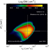 |
Fig. 22 Same as in Fig. 18, but at the age of ≈2000 yr for model W15-2-cw-IIb-HD+dec. The solid white cross marks the ranges of kTe and ne t of the bulk of the ejecta derived from Chandra X-ray observations of the SNR G292 (Bhalerao et al. 2019); the dashed lines mark the extreme values of kTe and ne t inferred for isolated knots in the northwest hemisphere of the remnant. |
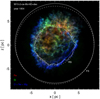 |
Fig. 23 Spatial distributions of EM of shocked Fe (red), Si (green), and intermediate-mass elements (O, Ne, and Mg; blue) integrated along the LoS (assuming the same orientation of G292) at the age of ≈ 2000 yr for model W15-2-cw-IIb-HD+dec. The solid contours mark the cuts of the forward and reverse shocks in the plane of the sky passing through the center of the explosion; the dashed lines mark the same cuts but for spheres with the centers coincident with the center of explosion (the cross) and radii corresponding to the average radii of the forward and reverse shocks. |
4 Discussion and conclusions
We presented 3D MHD and HD simulations which describe the formation of ejecta structure and asymmetries in the remnant of a neutrino-driven SN explosion. The aim was to explore how the morphology of the remnant and the structure of the ejecta keep memory of the asymmetries which developed stochastically by convective overturn in the neutrino-heating layer and by SASI activity during the first second after core bounce. To this end, we coupled the model of a neutrino-driven SN explosion with remarkable resemblance to basic properties of Cas A (Wongwathanarat et al. 2017) with MHD and HD simulations that describe the formation of the remnant (e.g., Orlando et al. 2016). The neutrino-driven SN model was presented and discussed in detail by Wongwathanarat et al. (2017). These authors showed that, in the considered model, three pronounced Ni-rich fingers grow, naturally but stochastically, due to HD instabilities. The initial seeds of these structures originate from the close proximity of the collapsed core right at the onset of the explosion (see Wongwathanarat et al. 2013, 2015), and their morphology suggests a correspondence to the extended shock-heated Fe-rich regions observed in Cas A.
Our 3D simulations start soon after the breakout of the shock wave at the stellar surface (≈ 20 h after core-collapse), using the output of the neutrino-driven SN simulation as initial condition. We performed SNR simulations either with or without the heating due to radioactive decay of 56Ni and 56Co (mainly effective during the first year of the evolution of the remnant) and simulations either with or without an ambient magnetic field. This specific exploration allowed us to evaluate the role played by these effects in the evolution of the ejecta and in determining their structure after the interaction of the reverse shock with the large-scale asymmetries left from the earliest phases of the explosion. The simulations covered ≈ 2000 yr of evolution. We compared the simulation results with the observations of Cas A, at the age of ≈ 350 yr and, tentatively, to the properties of the ≈3000 yr old SNR G292; at later epochs, we explored how and to which extent the remnant keeps memory of the anisotropies that emerged from violentnon-radial flows during the early moments after the core-collapse.
We found that our SNR models predict radii of the forward and reverse shocks and ejecta velocities at the age of ≈ 350 yr which are consistent (within the error bars) with those observed in Cas A (see Fig. 4), assuming a density of the stellar wind at the current position of the forward shock (nw = 0.8 cm−3) slightly lower than the best-fit value inferred from X-ray observations, but well within its uncertainty (nw = 0.9 ± 0.3 cm−3; Lee et al. 2014). We note that our models consider an ejecta mass (3.3 M⊙) in good agreement with the range of values estimated from the analysis of observations (Mej = [2−4] M⊙; e.g., Laming & Hwang 2003; Hwang & Laming 2003; Young et al. 2006), but assume an explosion energy (Eexp = 1.5 B) lower than expected for Cas A (≈ 2 B; Laming & Hwang 2003; Hwang & Laming 2003; Sato et al. 2020). A higher explosion energy would have produced a much better match of the models with the radii of the forward and reverse shocks and with the density of the stellar wind. Nevertheless, our models predict a mass of unshocked ejecta (≈ 0.85 M⊙) and, more specifically, unshocked Fe (≈0.068 M⊙) which are in excellent agreement with those recently inferred from the analysis of infrared observations (Laming & Temim 2020). Furthermore, our models allowed us to address the idea that the fundamental chemical, physical, and geometric properties observed in Cas A can naturally be explained in terms of the processes associated with the asymmetric beginning of a SN explosion and to a sequence of subsequent hydrodynamic instabilities that led to fragmentation and mixing in the ejecta. Our main findings are summarized as follows.
Formation of ring- and crown-like structures
The initial high-entropy plumes of Fe- and Ti-rich ejecta cross the reverse shock at the age of ≈ 30 yr. The slow-down of ejecta passing through the reverse shock triggers the development of HD instabilities (i.e., RT instability), which gradually fragment the plumes into numerous small-scale fingers. In this way, extended regions of shock-heated Fe form in the main shell of the remnant, which resemble those observed in Cas A. The pattern of small-scale structures in these regions reflects the ejecta structure left from the SN explosion. In fact, core-collapse SN simulations show the growth of fast plumes of Ni-rich ejecta into extended fingers from which fast metal-rich clumps can detach (e.g., Wongwathanarat et al. 2015). This leads to ejecta characterized by pronounced clumpiness with small dense clumps and knots mainly present at the tips of the high-entropy plumes (Wongwathanarat et al. 2017). The combination of these clumps and knots with the HD instabilities (that develop after the interaction of the ejecta with the reverse shock) naturally produces a filamentary pattern of shocked ejecta with ring-like features (see also Orlando et al. 2012, 2016). In many cases, the ring structures have RT fingers which extend outward, giving them the appearance of crowns. This effect is more evident in the case of denser fingers that can survive for a longer time (thus extending more outward) in the inter-shock region before they get dispersed due to mixing under the effect of RT and KH instabilities. In fact, the crown-like appearance is more evident in simulations including the decay heating (because of a higher density contrast of the ejecta at the tips of the plumes; see Fig. 9; see also Orlando et al. 2012) and it is also more evident when the effects of an ambient magnetic field are taken into account (because the field limits the growth of KH shear instability at the border of RT fingers; Mac Low et al. 1994; Fragile et al. 2005; Orlando et al. 2008). The resulting pattern of shocked ejecta in our models resembles that observed in Cas A remarkably well (DeLaney et al. 2010; Milisavljevic & Fesen 2013).
Inversion of ejecta layers
Our models show that the initial large-scale plumes also determine the spatial inversion of ejecta layers, leading to Fe-rich ejecta being located at greater radii than Si-rich ejecta. In fact, the inversion is evident only in regions where the fast plumes of Fe-rich ejecta interact with the reverse shock; elsewhere, the original chemical stratification is roughly preserved (see Fig. 9). The simulations show that, already at the breakout of the shock wave from the stellar surface, the fast plumes of Ni-rich ejecta led to a global metal asymmetry characterized by a deep penetration of Ni fingers into the overlying layers of the ejecta. After the decay of 56Ni to 56Co and of the latter to 56Fe, the Fe-rich plumes have protruded into the chemically distinct layers above and are enveloped by a less dense medium of Si-rich material. When the plumes start to interact with the reverse shock, the denser Fe-rich ejecta push the less dense Si-rich layer outward, breaking through it, and leading to the spatial inversion of the ejecta layers (see Fig. 9). The radioactive decay of Ni and Co enhances the effect of inversion of the ejecta layers. The additional pressure due to the decay heating inflates the Fe-rich fingers outward and sideways, making their outermost tips denser and more efficient in piercing the Si-rich layer. Another consequence of the dynamics of the fast and dense Fe-rich plumes is the accumulation of swept-out material of the outer layers (in particular Si) sideways around the shocked Fe regions (see Fig. 10). As a result, Fe-rich shocked regions are circled by rings of Si-rich shocked ejecta (see Figs. 8, B.2, and B.3). All these modeled features, namely the inversion of ejecta layers and the formation of Si-rich rings encircling the Fe-rich regions, nicely match those observed in Cas A (e.g., Hughes et al. 2000; DeLaney et al. 2010; Milisavljevic & Fesen 2013), suggesting that they are the fingerprints of the asymmetries that developed in the earliest phases of the SN explosion.
The “thick-disk” appearance
Discussing the orientation of the remnant structures compared to Cas A observations, we define the LoS such that the three dominant Fe-fingers coincide roughly with the directions where shocked Fe is seen in Cas A. In this case the kick motion of the CCO points to the southern hemisphere and toward the observer, in agreement with conclusions drawn from the distribution of 44Ti by Grefenstette et al. (2017). The simulations show that, in all cases, the metal-rich ejecta are arranged in a “thick-disk” geometry, with the disk tilted by an angle of ≈30° with respect to the plane of the sky (see Fig. 8). This is the natural consequence of the highly asymmetric explosion which ejected three dominant fast high-entropy plumes of metal-rich ejecta roughly lying in a plane tilted by ≈ 30°. The fast expansion of the three plumes makes the Si-, Ti-, and Fe-rich ejecta more expanded parallel to this plane than perpendicular to it, giving the metal-rich ejecta the appearance of a thick disk. Interestingly, also the ejecta of Cas A seem to be arranged in a thick disk which is tilted by an angle of ≈ 30° with respect to the plane of the sky (e.g., DeLaney et al. 2010; Grefenstette et al. 2017). Thus, the same initial large-scale asymmetry which produces the Fe-rich regions as in Cas A, the pattern of ring- and crown-like structures of the shocked ejecta, and the spatial inversion of ejecta layers as observed in Cas A, also predicts a thick-disk distribution of metal-rich ejecta with the same orientation as that observed in Cas A. When the decay heating is included, the tilted thick-disk appearance of Fe- and Ti-rich ejecta is slightly less evident. However, in this context it is worth noting that, in our models, we assumed that all of the decay energy is deposited in the ejecta without any γ-ray leakage from the inner part of the remnant. Our models, most likely, overestimate the effects of decay heating.
Formation of cavities and voids
The distribution of unshocked ejecta is characterized by cavities and voids. These are particularly evident in Si, Ti, and Fe. The largest cavities of Si correspond to the directions of propagation of the dominant Fe-rich plumes of ejecta. As a result, these cavities are located immediately below the regions of shocked Fe in the main shell of the remnant as evident by comparing Figs. 8 and 11 (see also Movie 2). Furthermore, the large cavities are physically connected with the large-scale Si-rich rings visible in the shocked ejecta and encircling the Fe-rich regions. As mentioned above, Si-rich layers of ejecta envelope the Fe-rich plumes. As one of these plumes passes through the reverse shock, a Fe-rich region encircled by Si-rich ejecta from the layer (both shock-heated and, therefore, visible in different bands) forms exterior to the shock, whereas a cavity in the unshocked Si (visible in the radio and near-infrared bands), which is filled by unshocked Fe (not visible), forms interior to the shock. This result naturally explains why the cavities in Si-rich ejecta observed in near-infrared observations of Cas A are physically connected to the bright rings in the main-shell (e.g., Milisavljevic & Fesen 2015). As suggested by Orlando et al. (2016), the cavities are actually filled by low-density unshocked Fe, which is not visible until it interacts with the reverse shock. In models including the decay heating, the cavities are more extended due to the inflation of the Fe-rich regions driven by the radioactive decay heating of the initial Ni. This effect enhances the size of the cavities and the formation of the large-scale Si-rich rings encircling the Fe-rich regions.
Distributions of 44Ti versus 56Fe
Our simulations show that, on average, Fe and Ti coexist in the mass-filled volume, according to the fact that these two species were synthesized in regions of Si burning and of processes like α-particle-rich freezeout, and later mixing cannot lead to any separation14. Nevertheless, we found that their abundance ratio can have significant variations (already at the initial conditions soon after the shock breakout at the stellar surface), with regions with a high concentration of Fe and others with a relatively high concentration of Ti. In particular, we found that the tips of the initial high-entropy plumes have, on average, a higher concentration of Fe. As a result, at the age of Cas A, the mass distributions of shocked and unshocked ejecta indicate that the former have, on average, a higher concentration of Fe, whereas the latter have, on average, a relatively higher concentration of Ti (see Fig. 13). The mass fraction ratio derived at the age of Cas A can vary by a factor of 10 around its average value (see Fig. 15). These results are fully consistent with the findings of Grefenstette et al. (2017) who found Ti-rich ejecta located both exterior and interior to the reverse shock from the analysis of NuSTAR observations. As in Cas A, in our models the bulk of shocked Ti is located in regions of shocked Fe, although there are also regions of shocked Fe with a low concentration of Ti. Grefenstette et al. (2017) claimed that Ti could not be found in Fe-forming regions if its abundance there is a factor of ≈ 2 lower than in the main Ti clumps. In fact, our models show that, at the center of regions of shocked Fe, the concentration of Fe is slightly higher and the concentration of Ti lower than on average even by factors larger than 2. According to our models, a significant amount of unshocked Fe is interior to the reverse shock (≈ 0.068 M⊙, in nice agreement with the recent findings of Laming & Temim 2020), preferentially concentrated in highly enriched clumps, which roughly form an irregular shell near the reverse shock, enclosing regions of more diluted Fe and Ti. We note that this unshocked Fe cannot be detected in Cas A until it is heated by the reverse shock. So, it is not astonishing that Ti is detected (emitting X-rays due to radioactive decay) in unshocked regions but not Fe. We found that the decay heating of Ni and Co does not affect the abundance ratio of Fe and Ti but can modify their spatial distributions. Regions with a high concentration of Ti (and a relatively lower concentration of Fe) do not expand as fast as regions with a higher Ni/Fe concentration, the latter expanding faster because of the additional pressure of the decay heating. In such a way, most of the Fe is pushed into the irregular shell of unshocked Fe close to the reverse shock, whereas regions with a high concentration of Ti remain (diluted) in the innermost part of the remnant. As a result, Ti-enriched regions appear more clearly offset from volumes with high Fe abundance in the case of effective decay heating.
Reverse shock asymmetry
The simulations show that the forward and reverse shocks deviate from a spherically symmetric expansion around the center of the explosion. Both shocks appear still roughly spherical (with small-scale deformations), but with an offset to the northwest by ≈ 0.13 pc from the center of the explosion. This offset is the consequence of the initial, asymmetric explosion, in which most of the Ni and Ti were ejected in the northern hemisphere away from the observer. Interestingly, observations of Cas A show that the geometric center of the reverse shock is offset to the northwest by ≈ 0.2 pc (at the distance of 3.4 kpc) from the center of the forward shock (Gotthelf et al. 2001). Our simulations cannot reproduce the offset between the two shocks, but suggest that, in general, the geometric center of the forward shock does not coincide with the center of the explosion. A similar offset can be also introduced if the remnant expands through a medium characterized by a global anisotropy (see upper left panel in Fig. 2 in Orlando et al. 2007). A direct consequence of this offset is that some caution should be applied when assuming the geometric center of the forward shock as the center of the explosion to estimate the kick velocity of a CCO. For instance, in the case of Cas A, the CCO travels in the southern hemisphere toward the observer, opposite to the offset of the forward and reverse shocks from the center of the explosion. Thus, assuming the geometric center of the forward shock as the center of the explosion lead to an overestimation of the kick velocity of the CCO. The velocities of the forward and reverse shocks in our models are in nice agreement with those inferred from the observations in the eastern and northern hemisphere of the remnant (e.g., Sato et al. 2018; Fesen et al. 2019). However, our simulations are not able to reproduce a reverse shock which appears to be stationary or even inward moving in the observer frame as suggested for Cas A by some authors (e.g., Helder & Vink 2008; Sato et al. 2018). The origin of this asymmetry is still debated in the literature and it is not clear if this is also connected with the offset between the centers of the forward and reverse shocks. A significant role can be played by environment asymmetries in the stellar wind (Orlando et al., in prep.).
The persistence of the explosion fingerprints at later times
Our simulations covered ≈2000 yr of evolution. During this time, most of the metal-rich ejecta have already crossed through the reverse shock and were subject to strong mixing by the HD instabilities. Nevertheless, the simulations show that the spatial distributions of Fe-group elements, Ti (or its decay product 44Ca), and Si still keep memory of the original SN asymmetry. Cavities and voids in the unshocked ejecta are still present even though they are much more diluted than in the epoch of Cas A. The fingerprints of the explosion are also evident in the asymmetric distributions of the velocity along the LoS for the various species. Even if our simulations were not tuned to the case of SNR G292, we compared our model results with multiwavelength observations of this remnant and found that some of the observed asymmetries may be interpreted in terms of large-scale asymmetries left from the earliest phases of the explosion, analogously to what we have found for Cas A. An accurate study of G292, however, would require dedicated simulations with ejecta mass, explosion energy, and structure of the ambient medium appropriate for this remnant.
In conclusion, our study has shown that the interaction of the reverse shock with the post-explosion large-scale asymmetries of the SN is fundamental for the formation of the structures observed in the inter-shock region of the remnant. The main aspects characterizing the shocked ejecta morphology of Cas A (Fe-rich regions, ring- and crown-like features, inversion of ejecta layers, etc.) form during the passage of the reverse shock from the environmental interaction, as a consequence of the fast growth of RT fingers in the reverse-shock heated material. The thick-disk appearance of the ejecta, the “bubble-like” structure of the unshocked ejecta, the distribution of Fe-group elements and Ti interior and exterior to the reverse shock, the asymmetries of the forward and reverse shocks, all these features encode the fingerprints of a neutrino-driven SN explosion.
However, a crucial aspect of the Cas A morphology was not accounted for by our simulations: the development of two Si-rich wide-angle jet-like features, visible in most of the wavelength bands. Some authors have claimed that these features might originate in magnetic jet-driven SNe (e.g., Khokhlov et al. 1999; Maeda & Nomoto 2003; Couch et al. 2009; Soker 2017; Grichener & Soker 2017; Bear & Soker 2018). In the case of Cas A, we suggest that they might originate from a post-explosion phenomenon that is not included in our simulations. For instance, an accretion disk of fallback matter could well have formed around the new-born neutron star (e.g., Chevalier 1989; Piro & Ott 2011). This possibility is supported by the inferred surface composition of the neutron star associated to Cas A, which is rich in carbon (Ho & Heinke 2009); a surface composition rich of light elements suggests a significant accretion after neutron-star formation. In this case, the fallback matter might have produced the jets by a mechanism similar to that responsible for the formation of jets in pulsars (e.g., Blackman & Perna 2004) or the early afterglows of γ-ray bursts (e.g., Dai & Liu 2012). In this context it is important to note that there are several 10−2 M⊙ of fallback in the SN model with plenty of angular momentum above the disk formation limit.
New simulations accounting for these additional phenomena are, therefore, necessary to shed light on the still pending questions of the origin of the many features observed in Cas A and in other SNRs. Finally, the analysis of multiwavelength observations aimed at reconstructing the 3D chemical distribution and structure of stellar debris in SNRs (e.g., DeLaney et al. 2010; Milisavljevic & Fesen 2013; Grefenstette et al. 2014, 2017; Milisavljevic & Fesen 2015; Abellán et al. 2017; Cigan et al. 2019; Law et al. 2020) and the comparison of model results with observations are essential steps to constrain the models and, therefore, to advance our understanding of the physical processes associated with SNe.
Movies
Movie of Fig. 7 Access here
Movie of Fig. 8 Access here
Movie of Fig. 12 Access here
Movie of Fig. 15 Access here
Acknowledgements
We thank the anonymous referee for useful suggestions that have allowed us to improve the paper. SO is grateful to A. Mignone for his support with the PLUTO code and his advises to consider a code configuration that minimizes the numerical diffusivity. The PLUTO code is developed at the Turin Astronomical Observatory (Italy) in collaboration with the Department of General Physics of Turin University (Italy) and the SCAI Department of CINECA (Italy). S.O., M.M., F.B. acknowledge financial contribution from the INAF mainstream program and from the agreement ASI-INAF n.2017-14-H.O. We acknowledge the “Accordo Quadro INAF-CINECA (2017)” and CINECA ISCRA Award N.HP10BARP6Y for the availability of high performance computing resources and support at the infrastructure Marconi based in Italy at CINECA. Additional computations were carried out at the SCAN (Sistema di Calcolo per l’Astrofisica Numerica) facility for high performance computing at INAF-Osservatorio Astronomico di Palermo. At Garching, funding by the European Research Council through grant ERC-AdG no. 341157-COCO2CASA and by the Deutsche Forschungsgemeinschaft (DFG, German Research Foundation) through Sonderforschungsbereich (Collaborative Research Centre) SFB-1258 “Neutrinos and Dark Matter in Astro- and Particle Physics (NDM)” and under Germany’s Excellence Strategy through Cluster of Excellence ORIGINS (EXC-2094)-390783311 is acknowledged. Computer resources for this project have been provided by the Max Planck Computing and Data Facility (MPCDF) on the HPC systems Cobra and Draco. S.N. is partially supported by “JSPS Grants-in-Aid for Scientific Research <KAKENHI > (A) 19H00693”, “Pioneering Program of RIKEN for Evolution of Matter in the Universe (r-EMU)”, and “Interdisciplinary Theoretical and Mathematical Sciences Program of RIKEN”. The navigable 3D graphics have been developed in the framework of the project 3DMAP-VR (3-Dimensional Modeling of Astrophysical Phenomena in Virtual Reality; Orlando et al. 2019b) at INAF-Osservatorio Astronomico di Palermo.
Appendix A Effects of radioactive decay and magnetic field on the mass distributions in velocity space
The effects of radioactive decay on the overall remnant evolution can be investigated by comparing the mass distributions of elements versus the radial and LoS velocities derived from models either with (model W15-2-cw-IIb-HD+dec) or without (model W15-2-cw-IIb-HD) decay heating. Figure A.1 shows these distributions at three epochs for model W15-2-cw-IIb-HD. The comparison of this figure with the analogous one derived from model W15-2-cw-IIb-HD+dec (Fig. 6) reveals that the fraction of Fe and Ti populating the high-velocity tail of their distributions is the highest if the decay heating is taken into account (compare left panels in Figs. A.1 and 6). Also, in model W15-2-cw-IIb-HD+dec, the tails of the fastest Fe and Ti stretch out the distributions to slightly higher velocities than in model W15-2-cw-IIb-HD.
The effects of decay heating are more evident in ejecta propagating away from us than in those propagating toward the observer. An inspection of the mass distributions versus the LoS velocities (right panels in Figs. A.1 and 6) shows that the main differences between models W15-2-cw-IIb-HD and W15-2-cw-IIb-HD+dec are concentrated in the redshifted part of the distributions. In fact the heating by radioactive decay provides an additional pressure source which inflates regions dominated by the decaying elements against their surroundings. As a result, the ejecta in the inflated regions expand faster than if the decay was not taken into account. The effect of decay are visible till the end of the simulations at the age of ≈ 2000 yr.
The effects of an ambient magnetic field on the remnant evolution can be investigated by comparing the mass distributions of elements derived from models either with (model W15-2-cw-IIb-MHD+dec) or without (model W15-2-cw-IIb-HD+dec) an ambient magnetic field. The comparison between Figs. 6 and A.2shows that the distributions in models W15-2-cw-IIb-HD+dec and W15-2-cw-IIb-MHD+dec are very similar with no relevant differences, indicating that the effects of magnetic field are negligible for the overall remnant evolution.
Appendix B Effects of radioactive decay and magnetic field on the spatial distribution of metal-rich ejecta
We investigated the effects of radioactive decay on spatial distribution of metal-rich ejecta by comparing model W15-2-cw-IIb-HD (without decay heating) with model W15-2-cw-IIb-HD+dec (including decay heating). Figure B.1 shows the spatial distribution of Fe at the time when the reverse shock reached the regions of Fe- and Ti-rich ejecta, about 30 yr after the SN event, for models W15-2-cw-IIb-HD (upper panels) and W15-2-cw-IIb-MHD+dec (lower panels). In this phase of evolution the Fe-rich plumes were not perturbed by the interaction with the reverse shock and the ejecta expanded almost homologously. However, bycomparing the Fe distribution derived from model W15-2-cw-IIb-HD (upper panel in Fig. B.1) with those derived from the other two models (upper panel in Fig. 7 and lower panels in Fig. B.1), we note that, in the latter two cases, the Fe-rich ejecta appear to be more swollen than in model W15-2-cw-IIb-HD (in which the Fe distribution is almost the same as in the initial condition). This difference is due to heating by radioactive decay of 56Ni and 56Co (species which populate the post-explosion instability-driven structures) that provide an additional gas pressure during the first year of evolution which inflates the Fe-rich plumes of ejecta.
At later times, the ejecta distribution keeps memory of the decay heating occurred during the first year of evolution. At the age of Cas A, the amount of shock-heated Fe is slightly higher if the decay heating is taken into account (see Fig. 5) due to the additional boost to the ejecta expansion provided by the heating. Furthermore the ring- and crown-like features of shocked ejecta are more developed in models W15-2-cw-IIb-HD+dec and W15-2-cw-IIb-MHD+dec than in model W15-2-cw-IIb-HD (compare Figs. 8 and B.3 with Fig. B.2). In fact, the decay heating increases the density contrast of Fe-rich fingers before they start to interact with the reverse shock. As a result they can penetrate more efficiently in the mixing region between the reverse and forward shocks (see also Orlando et al. 2012, 2016; Miceli et al. 2013; Tutone et al. 2020).
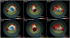 |
Fig. B.1 Same as the upper panels in Fig. 7, but for models W15-2-cw-IIb-HD (upper panels) and W15-2-cw-IIb-MHD+dec (lower panels). |
The shock-heated Fe-rich structures appear to be slightly more defined and extended in model W15-2-cw-IIb-MHD+dec than in W15-2-cw-IIb-HD+dec (compare Fig. B.3 with Fig. 8). In the former, the magnetic field limits the growth of HD instabilities that would develop at the borders of shocked clumps of ejecta through the tension of field lines which maintain a more laminar flow around the clump borders (e.g., Mac Low et al. 1994; Fragile et al. 2005; Orlando et al. 2008). As a result, the magnetic field limits the fragmentation by HD instabilities of the ring- and crown-like features of ejecta and makes them to survive for a longer time than those in model W15-2-cw-IIb-HD+dec, thus increasing their extension toward the forward shock (e.g., Orlando et al. 2012).
Appendix C Column density and emission measure distributions of 44Ti and 56Fe
Figure C.1 displays the column density maps of unshocked 56Fe and 44Ti (upper panels) and the corresponding distributions of EM of shocked species integrated along the LoS (lower panels) at the age of Cas A for our three models. The maps of shocked and unshocked ejecta are clearly dominated by Fe which, as expected, is more abundant than Ti. We note, however, that some regions show a prominent blue color both in shocked and unshocked ejecta, thus indicating that, along the LoS, either the EM of shocked Ti integrated along the LoS or the column density of unshocked Ti dominates over the corresponding distribution of Fe. This is particularly evident in the EM distributions of all models. In general, Ti-rich regions are located at the periphery of Fe-rich regions. There it would be easier to detect shock-heated Ti in high-energy observations. This is in agreement with NuSTAR observations that detected 44Ti exterior to the reverse shock in regions where shock-heated Fe is also detected (e.g., Grefenstette et al. 2017). Conversely, the cores of Fe-rich regions of shocked ejecta have a predominant red color, indicating that there the abundance of Fe is largely dominant over Ti and this may explain the evidence of regions where Fe but not 44Ti is detected in NuSTAR observations (e.g., Grefenstette et al. 2017).
 |
Fig. C.1 Upper panels: column density maps of unshocked Fe (red) and Ti (blue) at the age of Cas A for our three models. Lower panels: corresponding EM distributions of shocked Fe (red) and Ti (blue) integrated along the y-axis (i.e., the LoS assuming the vantage point at Earth). |
We also note that the structure of shock-heated Fe and Ti is the richest in models including the decay heating, because of the higher density contrast of Fe-rich plumes when they start to interact with the reverse shock (see Fig. 9). The heating is also responsible for the differences in the maps of column density of unshocked Fe and Ti: they appear much smoother in models with radioactive decay that in the model without. More bluish regions are evident in model W15-2-cw-IIb-HD, probably, because of the more clumpy structure of unshocked ejecta that allows to intercept regions with a higher concentration of 44Ti more easily along the LoS. We also note that model W15-2-cw-IIb-MHD+dec shows the highest abundance of Fe in the cores of Fe-rich regions of shocked ejecta (the regions appear more reddish). This is due, most likely, to a less mixing between layers of different chemical composition due to the presence of the magnetic field which limits the growth of HD instabilities which are responsible for the mixing (see Appendices A and B for the effects of decay heating and magnetic field on the evolution and structure of the ejecta).
References
- Abellán, F. J., Indebetouw, R., Marcaide, J. M., et al. 2017, ApJ, 842, L24 [NASA ADS] [CrossRef] [Google Scholar]
- Arias, M., Vink, J., de Gasperin, F., et al. 2018, A&A, 612, A110 [NASA ADS] [CrossRef] [EDP Sciences] [Google Scholar]
- Bear, E., & Soker, N. 2018, MNRAS, 478, 682 [NASA ADS] [Google Scholar]
- Bhalerao, J., Park, S., Dewey, D., et al. 2015, ApJ, 800, 65 [NASA ADS] [CrossRef] [Google Scholar]
- Bhalerao, J., Park, S., Schenck, A., Post, S., & Hughes, J. P. 2019, ApJ, 872, 31 [CrossRef] [Google Scholar]
- Blackman, E. G., & Perna, R. 2004, ApJ, 601, L71 [NASA ADS] [CrossRef] [Google Scholar]
- Blondin, J. M., & Ellison, D. C. 2001, ApJ, 560, 244 [NASA ADS] [CrossRef] [Google Scholar]
- Burrows, A., Radice, D., & Vartanyan, D. 2019, MNRAS, 485, 3153 [CrossRef] [Google Scholar]
- Chevalier, R. A. 1989, ApJ, 346, 847 [NASA ADS] [CrossRef] [Google Scholar]
- Chevalier, R. A., & Kirshner, R. P. 1978, ApJ, 219, 931 [NASA ADS] [CrossRef] [Google Scholar]
- Chevalier, R. A., & Oishi, J. 2003, ApJ, 593, L23 [NASA ADS] [CrossRef] [Google Scholar]
- Chevalier, R. A., Blondin, J. M., & Emmering, R. T. 1992, ApJ, 392, 118 [NASA ADS] [CrossRef] [Google Scholar]
- Cigan, P., Matsuura, M., Gomez, H. L., et al. 2019, ApJ, 886, 51 [NASA ADS] [CrossRef] [Google Scholar]
- Colella, P. 1990, J. Comput. Phys., 87, 171 [NASA ADS] [CrossRef] [Google Scholar]
- Couch, S. M., Wheeler, J. C., & Milosavljević, M. 2009, ApJ, 696, 953 [NASA ADS] [CrossRef] [Google Scholar]
- Dai, Z. G., & Liu, R.-Y. 2012, ApJ, 759, 58 [NASA ADS] [CrossRef] [Google Scholar]
- Dedner, A., Kemm, F., Kröner, D., et al. 2002, J. Comput. Phys., 175, 645 [Google Scholar]
- DeLaney, T., & Rudnick, L. 2003, ApJ, 589, 818 [NASA ADS] [CrossRef] [Google Scholar]
- DeLaney, T., Rudnick, L., Stage, M. D., et al. 2010, ApJ, 725, 2038 [NASA ADS] [CrossRef] [Google Scholar]
- DeLaney, T., Kassim, N. E., Rudnick, L., & Perley, R. A. 2014, ApJ, 785, 7 [NASA ADS] [CrossRef] [Google Scholar]
- Donati, J.-F., & Landstreet, J. D. 2009, ARA&A, 47, 333 [NASA ADS] [CrossRef] [MathSciNet] [Google Scholar]
- Dwek, E., Arendt, R. G., Bouchet, P., et al. 2010, ApJ, 722, 425 [NASA ADS] [CrossRef] [Google Scholar]
- Ferrand, G., Warren, D. C., Ono, M., et al. 2019, ApJ, 877, 136 [NASA ADS] [CrossRef] [Google Scholar]
- Ferrand, G., Warren, D. C., Ono, M., et al. 2021, ApJ, in press [arXiv:2011.04769] [Google Scholar]
- Fesen, R., Patnaude, D., Milisavljevic, D., Weil, K., & Brumback, M. 2019, in Supernova Remnants: An Odyssey in Space after Stellar Death II, invited talk, 3-8 June 2019, Chania, Crete, Greece, (online at http://snr2019.astro.noa.gr/index.php/program) [Google Scholar]
- Fragile, P. C., Anninos, P., Gustafson, K., & Murray, S. D. 2005, ApJ, 619, 327 [NASA ADS] [CrossRef] [Google Scholar]
- Frank, K. A., Zhekov, S. A., Park, S., et al. 2016, ApJ, 829, 40 [NASA ADS] [CrossRef] [Google Scholar]
- Fryxell, B., Mueller, E., & Arnett, D. 1991, ApJ, 367, 619 [NASA ADS] [CrossRef] [Google Scholar]
- Gabler, M., Wongwathanarat, A., & Janka, H.-T. 2020, MNRAS, submitted [arXiv:2008.01763] [Google Scholar]
- Gaensler, B. M., & Wallace, B. J. 2003, ApJ, 594, 326 [NASA ADS] [CrossRef] [Google Scholar]
- Gardiner, T. A., & Stone, J. M. 2005, J. Comput. Phys., 205, 509 [Google Scholar]
- Ghavamian, P., Hughes, J. P., & Williams, T. B. 2005, ApJ, 635, 365 [CrossRef] [Google Scholar]
- Ghavamian, P., Laming, J. M., & Rakowski, C. E. 2007, ApJ, 654, L69 [NASA ADS] [CrossRef] [Google Scholar]
- Gonzalez, M., & Safi-Harb, S. 2003, ApJ, 583, L91 [CrossRef] [Google Scholar]
- Gotthelf, E. V., Koralesky, B., Rudnick, L., et al. 2001, ApJ, 552, L39 [NASA ADS] [CrossRef] [Google Scholar]
- Greco, E., Vink, J., Miceli, M., et al. 2020, A&A, 638, A101 [CrossRef] [EDP Sciences] [Google Scholar]
- Grefenstette, B. W., Harrison, F. A., Boggs, S. E., et al. 2014, Nature, 506, 339 [NASA ADS] [CrossRef] [PubMed] [Google Scholar]
- Grefenstette, B. W., Fryer, C. L., Harrison, F. A., et al. 2017, ApJ, 834, 19 [NASA ADS] [CrossRef] [Google Scholar]
- Grichener, A., & Soker, N. 2017, MNRAS, 468, 1226 [NASA ADS] [CrossRef] [Google Scholar]
- Gull, S. F. 1973, MNRAS, 161, 47 [NASA ADS] [Google Scholar]
- Haberl, F., Geppert, U., Aschenbach, B., & Hasinger, G. 2006, A&A, 460, 811 [NASA ADS] [CrossRef] [EDP Sciences] [Google Scholar]
- Helder, E. A., Broos, P. S., Dewey, D., et al. 2013, ApJ, 764, 11 [NASA ADS] [CrossRef] [Google Scholar]
- Helder, E. A.,& Vink, J. 2008, ApJ, 686, 1094 [NASA ADS] [CrossRef] [Google Scholar]
- Ho, W. C. G.,& Heinke, C. O. 2009, Nature, 462, 71 [NASA ADS] [CrossRef] [PubMed] [Google Scholar]
- Holland-Ashford, T., Lopez, L. A., Auchettl, K., Temim, T., & Ramirez-Ruiz, E. 2017, ApJ, 844, 84 [NASA ADS] [CrossRef] [Google Scholar]
- Holland-Ashford, T., Lopez, L. A., & Auchettl, K. 2020, ApJ, 889, 144 [CrossRef] [Google Scholar]
- Hughes, J. P., Rakowski, C. E., Burrows, D. N., & Slane, P. O. 2000, ApJ, 528, L109 [NASA ADS] [CrossRef] [PubMed] [Google Scholar]
- Hughes, J. P., Slane, P. O., Park, S., Roming, P. W. A., & Burrows, D. N. 2003, ApJ, 591, L139 [NASA ADS] [CrossRef] [Google Scholar]
- Hwang, U., & Laming, J. M. 2003, ApJ, 597, 362 [NASA ADS] [CrossRef] [Google Scholar]
- Hwang, U., & Laming, J. M. 2012, ApJ, 746, 130 [NASA ADS] [CrossRef] [Google Scholar]
- Janka, H.-T. 2017, Handbook of Supernovae, eds. A. W. Alsabti, & P. Murdin (Switzerland: International Publishing), 1095 [CrossRef] [Google Scholar]
- Janka, H.-T., Melson, T., & Summa, A. 2016, Ann. Rev. Nucl. Part. Sci., 66, 341 [NASA ADS] [CrossRef] [Google Scholar]
- Jeffery, D. J. 1999, ArXiv e-prints [arXiv:astro-ph/9907015] [Google Scholar]
- Jun, B.-I., & Norman, M. L. 1996a, ApJ, 465, 800 [NASA ADS] [CrossRef] [Google Scholar]
- Jun, B.-I., & Norman, M. L. 1996b, ApJ, 472, 245 [NASA ADS] [CrossRef] [Google Scholar]
- Kamper, K., & van den Bergh, S. 1976, ApJS, 32, 351 [NASA ADS] [CrossRef] [Google Scholar]
- Katsuda, S., Morii, M., Janka, H.-T., et al. 2018, ApJ, 856, 18 [NASA ADS] [CrossRef] [Google Scholar]
- Khokhlov, A. M., Höflich, P. A., Oran, E. S., et al. 1999, ApJ, 524, L107 [NASA ADS] [CrossRef] [Google Scholar]
- Koo, B.-C., Kim, H.-J., Lee, Y.-H., et al. 2018, ApJ, 866, 139 [CrossRef] [Google Scholar]
- Koo, B.-C., Kim, H.-J., Oh, H., et al. 2020, Nat. Astron., 4, 584 [CrossRef] [Google Scholar]
- Krause, O., Birkmann, S. M., Usuda, T., et al. 2008, Science, 320, 1195 [NASA ADS] [CrossRef] [PubMed] [Google Scholar]
- Laming, J. M., & Hwang, U. 2003, ApJ, 597, 347 [NASA ADS] [CrossRef] [Google Scholar]
- Laming, J. M., & Temim, T. 2020, ApJ, 904, 115 [CrossRef] [Google Scholar]
- Larsson, J., Fransson, C., Östlin, G., et al. 2011, Nature, 474, 484 [NASA ADS] [CrossRef] [PubMed] [Google Scholar]
- Law, C. J., Milisavljevic, D., Patnaude, D. J., et al. 2020, ApJ, 894, 73 [CrossRef] [Google Scholar]
- Lawrence, S. S., MacAlpine, G. M., Uomoto, A., et al. 1995, AJ, 109, 2635 [NASA ADS] [CrossRef] [Google Scholar]
- Lawrence, S. S., Sugerman, B. E., Bouchet, P., et al. 2000, ApJ, 537, L123 [NASA ADS] [CrossRef] [Google Scholar]
- Lee, J.-J., Park, S., Hughes, J. P., & Slane, P. O. 2014, ApJ, 789, 7 [NASA ADS] [CrossRef] [Google Scholar]
- Lopez, L. A., & Fesen, R. A. 2018, Space Sci. Rev., 214, 44 [CrossRef] [Google Scholar]
- Lopez, L. A., Ramirez-Ruiz, E., Huppenkothen, D., Badenes, C., & Pooley, D. A. 2011, ApJ, 732, 114 [NASA ADS] [CrossRef] [Google Scholar]
- Mac Low, M., McKee, C. F., Klein, R. I., Stone, J. M., & Norman, M. L. 1994, ApJ, 433, 757 [NASA ADS] [CrossRef] [Google Scholar]
- Maeda, K., & Nomoto, K. 2003, ApJ, 598, 1163 [NASA ADS] [CrossRef] [Google Scholar]
- Magkotsios, G., Timmes, F. X., Hungerford, A. L., et al. 2010, ApJS, 191, 66 [NASA ADS] [CrossRef] [Google Scholar]
- Miceli, M., Decourchelle, A., Ballet, J., et al. 2006, A&A, 453, 567 [NASA ADS] [CrossRef] [EDP Sciences] [Google Scholar]
- Miceli, M., Orlando, S., Reale, F., Bocchino, F., & Peres, G. 2013, MNRAS, 430, 2864 [NASA ADS] [CrossRef] [Google Scholar]
- Mignone, A., Plewa, T., & Bodo, G. 2005, ApJS, 160, 199 [NASA ADS] [CrossRef] [Google Scholar]
- Mignone, A., Bodo, G., Massaglia, S., et al. 2007, ApJS, 170, 228 [Google Scholar]
- Mignone, A., Tzeferacos, P., & Bodo, G. 2010, J. Comput. Phys., 229, 5896 [NASA ADS] [CrossRef] [Google Scholar]
- Mignone, A., Zanni, C., Tzeferacos, P., et al. 2012, ApJS, 198, 7 [Google Scholar]
- Milisavljevic, D., & Fesen, R. A. 2013, ApJ, 772, 134 [NASA ADS] [CrossRef] [Google Scholar]
- Milisavljevic, D., & Fesen, R. A. 2015, Science, 347, 526 [NASA ADS] [CrossRef] [Google Scholar]
- Milisavljevic, D., & Fesen, R. A. 2017, Handbook of Supernovae, eds. A. W. Alsabti, & P. Murdin, (Switzerland: Springer International Publishing), 2211 [CrossRef] [Google Scholar]
- Nadyozhin, D. K. 1994, ApJS, 92, 527 [Google Scholar]
- Nagataki, S. 2000, ApJS, 127, 141 [NASA ADS] [CrossRef] [Google Scholar]
- Nagataki, S., Hashimoto, M., Sato, K., & Yamada, S. 1997, ApJ, 486, 1026 [NASA ADS] [CrossRef] [Google Scholar]
- Nagataki, S., Hashimoto, M.-a., Sato, K., Yamada, S., & Mochizuki, Y. S. 1998, ApJ, 492, L45 [NASA ADS] [CrossRef] [Google Scholar]
- O’Connor, E. P., & Couch, S. M. 2018, ApJ, 865, 81 [NASA ADS] [CrossRef] [Google Scholar]
- Ono, M., Nagataki, S., Ito, H., et al. 2013, ApJ, 773, 161 [NASA ADS] [CrossRef] [Google Scholar]
- Ono, M., Nagataki, S., Ferrand, G., et al. 2020, ApJ, 888, 111 [NASA ADS] [CrossRef] [Google Scholar]
- Orlando, S., Bocchino, F., Reale, F., Peres, G., & Petruk, O. 2007, A&A, 470, 927 [NASA ADS] [CrossRef] [EDP Sciences] [Google Scholar]
- Orlando, S., Bocchino, F., Reale, F., Peres, G., & Pagano, P. 2008, ApJ, 678, 274 [NASA ADS] [CrossRef] [Google Scholar]
- Orlando, S., Bocchino, F., Miceli, M., Petruk, O., & Pumo, M. L. 2012, ApJ, 749, 156 [NASA ADS] [CrossRef] [Google Scholar]
- Orlando, S., Miceli, M., Pumo, M. L., & Bocchino, F. 2015, ApJ, 810, 168 [NASA ADS] [CrossRef] [Google Scholar]
- Orlando, S., Miceli, M., Pumo, M. L., & Bocchino, F. 2016, ApJ, 822, 22 [NASA ADS] [CrossRef] [Google Scholar]
- Orlando, S., Miceli, M., Petruk, O., et al. 2019a, A&A, 622, A73 [NASA ADS] [CrossRef] [EDP Sciences] [Google Scholar]
- Orlando, S., Pillitteri, I., Bocchino, F., Daricello, L., & Leonardi, L. 2019b, Res. Notes AAS, 3, 176 [CrossRef] [Google Scholar]
- Orlando, S., Ono, M., Nagataki, S., et al. 2020, A&A, 636, A22 [CrossRef] [EDP Sciences] [Google Scholar]
- Park, S., Roming, P. W. A., Hughes, J. P., et al. 2002, ApJ, 564, L39 [NASA ADS] [CrossRef] [Google Scholar]
- Park, S., Hughes, J. P., Slane, P. O., et al. 2004, ApJ, 602, L33 [NASA ADS] [CrossRef] [Google Scholar]
- Park, S., Hughes, J. P., Slane, P. O., et al. 2007, ApJ, 670, L121 [NASA ADS] [CrossRef] [Google Scholar]
- Parker, E. N. 1958, ApJ, 128, 664 [Google Scholar]
- Patnaude, D. J., & Fesen, R. A. 2009, ApJ, 697, 535 [NASA ADS] [CrossRef] [Google Scholar]
- Piro, A. L., & Ott, C. D. 2011, ApJ, 736, 108 [NASA ADS] [CrossRef] [Google Scholar]
- Pllumbi, E. 2015, PhD thesis (Technische Universität München), Germany [Google Scholar]
- Raymond, J. C., Koo, B. C., Lee, Y. H., et al. 2018, ApJ, 866, 128 [CrossRef] [Google Scholar]
- Reed, J. E., Hester, J. J., Fabian, A. C., & Winkler, P. F. 1995, ApJ, 440, 706 [NASA ADS] [CrossRef] [Google Scholar]
- Rest, A., Foley, R. J., Sinnott, B., et al. 2011, ApJ, 732, 3 [NASA ADS] [CrossRef] [Google Scholar]
- Sato, T., Katsuda, S., Morii, M., et al. 2018, ApJ, 853, 46 [NASA ADS] [CrossRef] [Google Scholar]
- Sato, T., Yoshida, T., Umeda, H., et al. 2020, ApJ, 893, 49 [CrossRef] [Google Scholar]
- Soker, N. 2017, Res. Astron. Astrophys., 17, 113 [NASA ADS] [CrossRef] [Google Scholar]
- Timmes, F. X., & Swesty, F. D. 2000, ApJS, 126, 501 [NASA ADS] [CrossRef] [Google Scholar]
- Tutone, A., Orlando, S., Miceli, M., et al. 2020, A&A, 642, A67 [CrossRef] [EDP Sciences] [Google Scholar]
- Utrobin, V. P., Wongwathanarat, A., Janka, H. T., et al. 2019, A&A, 624, A116 [NASA ADS] [CrossRef] [EDP Sciences] [Google Scholar]
- Vance, G. S., Young, P. A., Fryer, C. L., & Ellinger, C. I. 2020, ApJ, 895, 82 [CrossRef] [Google Scholar]
- Wang, C.-Y., & Chevalier, R. A. 2001, ApJ, 549, 1119 [NASA ADS] [CrossRef] [Google Scholar]
- Weil, K. E., Fesen, R. A., Patnaude, D. J., et al. 2020, ApJ, 891, 116 [CrossRef] [Google Scholar]
- Willingale, R., Bleeker, J. A. M., van der Heyden, K. J., Kaastra, J. S., & Vink, J. 2002, A&A, 381, 1039 [NASA ADS] [CrossRef] [EDP Sciences] [Google Scholar]
- Winkler, P. F., Twelker, K., Reith, C. N., & Long, K. S. 2009, ApJ, 692, 1489 [NASA ADS] [CrossRef] [Google Scholar]
- Wongwathanarat, A., Janka, H.-T., & Müller, E. 2010, ApJ, 725, L106 [NASA ADS] [CrossRef] [Google Scholar]
- Wongwathanarat, A., Janka, H. T., & Müller, E. 2013, A&A, 552, A126 [NASA ADS] [CrossRef] [EDP Sciences] [Google Scholar]
- Wongwathanarat, A., Müller, E., & Janka, H.-T. 2015, A&A, 577, A48 [NASA ADS] [CrossRef] [EDP Sciences] [Google Scholar]
- Wongwathanarat, A., Janka, H.-T., Müller, E., Pllumbi, E., & Wanajo, S. 2017, ApJ, 842, 13 [NASA ADS] [CrossRef] [Google Scholar]
- Woosley, S. E., & Weaver, T. A. 1995, ApJS, 101, 181 [NASA ADS] [CrossRef] [Google Scholar]
- Yang, X.-J., Liu, X.-Q., Li, S.-Y., & Lu, F.-J. 2014, Res. Astron. Astrophys., 14, 1279 [CrossRef] [Google Scholar]
- Young, P. A., Fryer, C. L., Hungerford, A., et al. 2006, ApJ, 640, 891 [NASA ADS] [CrossRef] [Google Scholar]
- Zanardo, G., Staveley-Smith, L., Ball, L., et al. 2010, ApJ, 710, 1515 [NASA ADS] [CrossRef] [Google Scholar]
A unique exception is SN 1987A whose remnant was resolved about ten years after the SN event thanks to observations in different wavelength bands, from radio (e.g., with the Australia Telescope Compact Array, Zanardo et al. 2010), to infrared (e.g., with Spitzer, Dwek et al. 2010), to optical (e.g., with Hubble Space Telescope, Lawrence et al. 2000; Larsson et al. 2011), to X-ray bands (e.g., with Chandra and XMM-Newton, Haberl et al. 2006; Helder et al. 2013; Frank et al. 2016).
The evidence that species as Si, S, Ar, and Ca are predominantly ejected opposite to the direction of neutron star motion is common to many core-collapse SNRs, as inferred from the analysis of a sample of remnants observed with Chandra and XMM-Newton (e.g., Holland-Ashford et al. 2017; Katsuda et al. 2018).
We compared the gas potential energy per unit of mass of each grid cell with its kinetic energy per unit of mass and found that the ratio of kinetic energy to potential energy is much higher than one for all the expanding ejecta. This holds also at the time of the mapping from the SN to the SNR simulation, except for a small number of cells near the very center of the spatial domain (namely some cells close to the explosion center), which, however, contain only very little mass.
Some authors considered the wind as that of a red supergiant progenitor (e.g., Chevalier & Oishi 2003; Lee et al. 2014; Weil et al. 2020). However, after the outer H envelope of the progenitor star was stripped away, we do not expect the remaining star to be a red supergiant. In fact, Koo et al. (2020) recently suggested a scenario in which Cas A resulted from a type IIb supernova explosion of a blue supergiant with a thin H envelope.
After the removal of the H envelope, the pre-SN star of our simulations has a radius of ≈ 21.4 R⊙ at collapse (see model W15-IIb in Wongwathanarat et al. 2017).
Apart from the explosion mechanism, the properties of these asymmetries also depend on the density structure of the progenitor star (e.g., Wongwathanarat et al. 2015).
According to simulations of core-collapse SNe, the occurrence of three large plumes is quite common in the case of highly asymmetrical explosions, though in some cases a single plume (large dipole asymmetry of the explosion) or two large plumes (bipolar structure) may develop (e.g., Wongwathanarat et al. 2013, 2015; Utrobin et al. 2019, and in prep.).
As mentioned in Sect. 3.1, here we considered only 56Fe from 56Ni decay. The Fe mass, therefore, is underestimated by about 10% (e.g., Wongwathanarat et al. 2017). Additional mass comes from other isotopes as 52Fe.
The mass was estimated by considering the results of the tracer-particle-based post-processing with the large nuclear network (Wongwathanarat et al. 2017), but not considering the decay of 44Ti in 44Ca. At the age of Cas A, the density of 44Ti is scaled by a factor of 0.027, for an e-folding time of 90 yr.
The hole in the shell evident in the lower panels in Fig. 7 forms because the bulk of Fe-rich ejecta, denser than 5% of the peak density of Fe, has not reached yet the reverse shock.
All Tables
All Figures
|
Fig. 1 Isosurfaces of mass fractions of |
| In the text | |
|
Fig. 2 Mass distribution of selected species versus the ratio |
| In the text | |
|
Fig. 3 Mass distributions of 1H, 4He, 12C, 16O, 28Si, 44Ti, and the quantity |
| In the text | |
|
Fig. 4 Angle-averaged radii of the forward (red lines) and reverse (blue lines) shocks versus time for the three models investigated. The black crosses show the corresponding observational values at the current age of Cas A (Gotthelf et al. 2001); the vertical lines of the crosses show the observational uncertainty. |
| In the text | |
|
Fig. 5 Mass of shocked Si (green lines), Ti (blue), and Fe (red) normalized to their total mass versus time for the three SNR modelsanalyzed. The vertical black line marks the age of Cas A. |
| In the text | |
|
Fig. 6 Mass distributions of 1H, 4He, 12C, 16O, 28Si, 44Ti, and 56Fe versus radialvelocity, vrad (left panels), and velocity component along the LoS, vLoS (right panels) at the labeled times for model W15-2-cw-IIb-HD+dec. The upper panels correspond to the time when Fe and Ti start to interact with the reverse shock, the middle panels to the time corresponding to the age of Cas A, and the lower panels to t ≈ 2000 yr. |
| In the text | |
|
Fig. 7 Isosurfaces of the distribution of Fe at the time when the reverse shock starts to interact with the Fe- and Ti-rich plumes of ejecta (upper panels), at the age of Cas A (middle panels), and at t = 2000 yr (lower panels) for different viewing angles (from left to right) for model W15-2-cw-IIb-HD+dec. The opaque irregular isosurfaces correspond to a value of Fe density which is at 5% of the peak density; their colors give the radial velocity in units of 1000 km s−1 on the isosurface (the color coding is defined at the bottom of each panel). The semi-transparent clipped quasi-spherical surfaces indicate the forward (green) and reverse (yellow) shocks. The Earth vantage point lies on the negative y-axis. See online Movie 1foran animation of these data; a navigable 3D graphic of the Fe spatial distribution at the age of Cas A is available at https://skfb.ly/6TKRK. |
| In the text | |
|
Fig. 8 Isosurfaces of the distributions of shocked Fe (red) and Si (green) at the age of Cas A for different viewing angles for model W15-2-cw-IIb-HD+dec. The upper left panel corresponds to the vantage point at Earth for Cas A. The opaque irregular isosurfaces correspond to a value of Fe and Si density which is at 25% of the respective peak density. The semi-transparent white surface indicates the reverse shock. See online Movie 2 for an animation of these data; a navigable 3D graphic of these distributions which includes also unshocked Fe and Si is available at https://skfb.ly/6UJYu. |
| In the text | |
|
Fig. 9 Radial profiles of Fe (red), Ti (blue), and Si (green) averaged over a solid angle of 30° in the direction of the east Fe-rich finger (roughly along the negative x-axis in the left panels of Fig. 7; solid lines) and of the negative z-axis (i.e., where no Fe-rich finger is present; dashed lines) for our three models, at three different epochs. The vertical dotted line in each panel marks the average position of the reverse shock. The density of Ti was calculated by considering the tracer-particle-based post-processing with a large nuclear network (Wongwathanarat et al. 2017), but not considering its decay in 44Ca (for an e-folding time of 90 yr, the Ti density is scaled by a factor of 0.027). |
| In the text | |
|
Fig. 10 Profiles of Fe (red), Ti (blue), and Si (green) as a function of the distance from the center of the Fe finger that roughly points to the east (top row), to the west (middle row) and to the north (botton row), at the age of Cas A, for our three models. The profiles are averaged over all directions in a plane tangential to the sphere at r ≈ 0.7 Rfs from the center of the explosion (namely immediately above the reverse shock). The density of Ti was calculated by considering the tracer-particle-based post-processing with a large nuclear network (Wongwathanarat et al. 2017), but not considering its decay in 44Ca (for an e-folding time of 90 yr, the Ti density is scaled by a factor of 0.027). The inset in the lower left corner of each panel shows a three-color composite image of the mass density distributions of Fe (red), Ti (blue), and Si (green) in the plane at r ≈ 0.7 Rfs. |
| In the text | |
|
Fig. 11 Isosurfaces of the distributions of unshocked Fe (red) and Si (green) at the age of Cas A for different viewing angles (from left to right) for model W15-2-cw-IIb-HD+dec. The left panels correspond to the observer direction for Cas A. The isosurfaces enclose 50% (upper row), 75% (center row), and 95% (lower row) of the total mass of unshocked Fe and Si and correspond to a value of Fe (Si) density, in units of 10−26 g cm−3, which is 81 (25), 70 (16), and 55 (6.0), respectively. |
| In the text | |
|
Fig. 12 Isosurfaces of the distributions of unshocked Fe (red) and Ti (blue) at the age of Cas A for different values of the mass fractions (decreasing from left to right; see the values reported at the end of the caption) and different viewing angles (front and side views) for models W15-2-cw-IIb-HD and W15-2-cw-IIb-HD+dec. The values of the mass fractions are selected so that the corresponding isosurfaces enclose, from left to right, 30, 50, 75, and 95% of the total mass of the respective unshocked species. The red isosurfaces correspond to a value of Fe density in model W15-2-cw-IIb-HD (W15-2-cw-IIb-HD+dec) which is, in units of 10−26 g cm−3, 119 (89), 95 (81), 71 (70), 40 (55), respectively; the blue isosurfaces correspond to a value ofTi density in model W15-2-cw-IIb-HD (W15-2-cw-IIb-HD+dec) which is, in units of 10−27 g cm−3 (considering the tracer-particle-based post-processing with a large nuclear network, Wongwathanarat et al. 2017, but not considering its decay in 44Ca), 2.1 (1.7), 1.7 (1.4), 1.2 (1.1), 0.7 (0.8), respectively (considering the decay of 44Ti in 44Ca, these values are scaled by a factor of 0.027, for an e-folding time of 90 yr). See online Movie 3 for an animation of these data; a navigable 3D graphic of these distributions is available at https://skfb.ly/6UMxI. |
| In the text | |
|
Fig. 13 Mass distribution of Si (green), Ti (blue), and Fe (red) versus the ratio |
| In the text | |
|
Fig. 14 Same as in Fig. 12, but for the distributions of shocked Fe (red) and Ti (blue). The values of the mass fractions are selected so that the corresponding isosurfaces enclose, from left to right, 50, 75, and 95% of the total mass of the respective shocked species. The red isosurfaces correspond to a value of Fe density in model W15-2-cw-IIb-HD (W15-2-cw-IIb-HD+dec) which is, in units of 10−25 g cm−3, 72 (50), 35 (26), 7.5 (7.9), respectively; the blue isosurfaces correspond to a value of Ti density in model W15-2-cw-IIb-HD (W15-2-cw-IIb-HD+dec) which is, in units of 10−26 g cm−3 (considering the tracer-particle-based post-processing with a large nuclear network, Wongwathanarat et al. 2017, but not considering its decay in 44Ca), 21 (15), 10 (7.9), 2.8 (2.5), respectively (considering the decay of 44Ti in 44Ca, these values are scaled by a factor of 0.027, for an e-folding time of 90 yr). A navigable 3D graphic of these distributions is available at https://skfb.ly/6UMxI. |
| In the text | |
|
Fig. 15 3D distributions of mass fraction ratio [CFe∕CTi] (upper 2 rows) and log of abundance ratio, |
| In the text | |
|
Fig. 16 Emission measure, EM, of shocked Fe (red) and Si (green) integrated along the y-axis (i.e., the LoS assuming the vantage point at Earth), and column density, nTi, of Ti (both shocked and unshocked; blue) at the age of Cas A for our three models. The solid contours mark cuts of the forward andreverse shocks in the plane of the sky passing through the center of the explosion; the dashed lines mark the same cuts but for spheres with the centers coincident with the center of explosion and radii corresponding to the average radii of the forward and reverse shocks. The two crosses in each panel mark the center of the explosion and the geometric center of the forward and reverse shocks offset to the northwest. |
| In the text | |
|
Fig. 17 Forward (black) and reverse (red) shock velocities versus the position angle in the plane of the sky for model W15-2-cw-IIb-HD+dec at the age of Cas A. The dashed horizontal lines mark the median values of the respective velocities. The shaded area marks the position angle where the reverse shock appears to be stationary or even moving inward in observations of Cas A (e.g., Helder & Vink 2008; Sato et al. 2018). |
| In the text | |
|
Fig. 18 Distribution of emission measure versus electron temperature (kTe) and ionization age (net) at the epoch of Cas A derived from model W15-2-cw-IIb-HD+dec compared with the results of Chandra X-ray observations. The large white cross marks the ranges of kTe and ne t derived from an X-ray survey of ejecta in Cas A (Hwang & Laming 2012); the small yellow crosses mark the values inferred from the analysis of regions dominated by thermal emission of shocked ambient gas (Lee et al. 2014). |
| In the text | |
|
Fig. 19 Maps of average EM-weighted velocity along the LoS for shocked Si (upper panel) and Fe (lower panel) at the age of Cas A for model W15-2-cw-IIb-HD+dec. The approximate velocity range is ± 5000 km s−1 (see color bar on the right in units of 1000 km s−1). The solid contours mark the cuts of the forward and reverse shocks in the plane of the sky passing through the center of the explosion. These images correspond to the effective Doppler maps derived from observations. |
| In the text | |
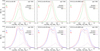 |
Fig. 20 Same as in Fig. 13, but at the age of ≈2000 yr. |
| In the text | |
|
Fig. 21 Isosurface of the distribution of Fe at t = 2000 yr for model W15-2-cw-IIb-HD+dec. The model is oriented to roughly match the direction of the neutron star kick and the remnant asymmetries observed in G292. The opaque corrugated isosurface corresponds to a value of the Fe density which is at 5% of the peak density; the colors give the radial velocity in units of 1000 km s−1 on the isosurface (the color coding is defined at the bottom of the panel). The semi-transparent quasi-spherical surface indicates the forward shock. The Earth vantage point lies on the negative y-axis. |
| In the text | |
|
Fig. 22 Same as in Fig. 18, but at the age of ≈2000 yr for model W15-2-cw-IIb-HD+dec. The solid white cross marks the ranges of kTe and ne t of the bulk of the ejecta derived from Chandra X-ray observations of the SNR G292 (Bhalerao et al. 2019); the dashed lines mark the extreme values of kTe and ne t inferred for isolated knots in the northwest hemisphere of the remnant. |
| In the text | |
|
Fig. 23 Spatial distributions of EM of shocked Fe (red), Si (green), and intermediate-mass elements (O, Ne, and Mg; blue) integrated along the LoS (assuming the same orientation of G292) at the age of ≈ 2000 yr for model W15-2-cw-IIb-HD+dec. The solid contours mark the cuts of the forward and reverse shocks in the plane of the sky passing through the center of the explosion; the dashed lines mark the same cuts but for spheres with the centers coincident with the center of explosion (the cross) and radii corresponding to the average radii of the forward and reverse shocks. |
| In the text | |
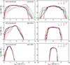 |
Fig. A.1 Same as in Fig. 6, but for model W15-2-cw-IIb-HD. |
| In the text | |
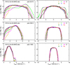 |
Fig. A.2 Same as in Fig. 6, but for model W15-2-cw-IIb-MHD+dec. |
| In the text | |
|
Fig. B.1 Same as the upper panels in Fig. 7, but for models W15-2-cw-IIb-HD (upper panels) and W15-2-cw-IIb-MHD+dec (lower panels). |
| In the text | |
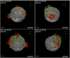 |
Fig. B.2 Same as in Fig. 8, but for model W15-2-cw-IIb-HD. |
| In the text | |
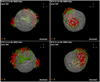 |
Fig. B.3 Same as in Fig. 8, but for model W15-2-cw-IIb-MHD+dec. |
| In the text | |
|
Fig. C.1 Upper panels: column density maps of unshocked Fe (red) and Ti (blue) at the age of Cas A for our three models. Lower panels: corresponding EM distributions of shocked Fe (red) and Ti (blue) integrated along the y-axis (i.e., the LoS assuming the vantage point at Earth). |
| In the text | |
Current usage metrics show cumulative count of Article Views (full-text article views including HTML views, PDF and ePub downloads, according to the available data) and Abstracts Views on Vision4Press platform.
Data correspond to usage on the plateform after 2015. The current usage metrics is available 48-96 hours after online publication and is updated daily on week days.
Initial download of the metrics may take a while.