| Issue |
A&A
Volume 644, December 2020
|
|
|---|---|---|
| Article Number | A111 | |
| Number of page(s) | 13 | |
| Section | Cosmology (including clusters of galaxies) | |
| DOI | https://doi.org/10.1051/0004-6361/202038586 | |
| Published online | 08 December 2020 | |
From universal profiles to universal scaling laws in X-ray galaxy clusters
1
INAF, Osservatorio di Astrofisica e Scienza dello Spazio, via Pietro Gobetti 93/3, 40129 Bologna, Italy
e-mail: This email address is being protected from spambots. You need JavaScript enabled to view it.
2
INFN, Sezione di Bologna, viale Berti Pichat 6/2, 40127 Bologna, Italy
3
Center for Astrophysics | Harvard & Smithsonian, 60 Garden Street, Cambridge, MA 02138, USA
Received:
5
June
2020
Accepted:
6
October
2020
Abstract
As the end products of the hierarchical process of cosmic structure formation, galaxy clusters present some predictable properties, like those mostly driven by gravity, and some others more affected by astrophysical dissipative processes that can be recovered from observations and that show remarkable universal behaviour once rescaled by halo mass and redshift. However, a consistent picture that links these universal radial profiles and the integrated values of the thermodynamical quantities of the intracluster medium, also quantifying the deviations from the standard self-similar gravity-driven scenario, has to be demonstrated. In this work we use a semi-analytic model based on a universal pressure profile in hydrostatic equilibrium within a cold dark matter halo with a defined relation between mass and concentration to reconstruct the scaling laws between the X-ray properties of galaxy clusters. We also quantify any deviation from the self-similar predictions in terms of temperature dependence of a few physical quantities such as the gas mass fraction, the relation between spectroscopic temperature and its global value, and, if present, the hydrostatic mass bias. This model allows us to reconstruct both the observed profiles and the scaling laws between integrated quantities. We use the Planck Early Sunyaev-Zeldovich sample, a Planck-selected sample of objects homogeneously analysed in X-rays, to calibrate the predicted scaling laws between gas mass, temperature, luminosity, and total mass. Our universal model reproduces well the observed thermodynamic properties and provides a way to interpret the observed deviations from the standard self-similar behaviour, also allowing us to define a framework to modify accordingly the characteristic physical quantities that renormalise the observed profiles. By combining these results with the constraints on the observed YSZ − T relation we show how we can quantify the level of gas clumping affecting the studied sample, estimate the clumping-free gas mass fraction, and suggest the average level of hydrostatic bias present.
Key words: galaxies: clusters: general / galaxies: clusters: intracluster medium / X-rays: galaxies: clusters
© ESO 2020
1. Introduction
Galaxy clusters are cosmological objects that form by hierarchical aggregation of matter under the action of the gravity force. As a consequence of this force the clusters have physical properties that scale to the mass and redshift of the dark matter halo (e.g. Kaiser 1986; Böhringer et al. 2012; Kravtsov & Borgani 2012). This is true not only for their total gravitating mass, but also for observational quantities that depend mostly on the depth of the potential well, like the temperature of the intracluster medium, which indicates how much most of the baryons collapsed in a dark matter halo are heated by the accretion shocks.
Where the physical processes of aggregation and collapse are dominated by the gravity, a set of relations emerges from this self-similar scenario between the global quantities (i.e. integrated over the volume) that describe the observed properties of the galaxy clusters, such as gas temperature, luminosity, mass, and total mass. However, a predictable behaviour is also expected to hold in how these quantities vary with the radial distance from the bottom of the potential well, in particular in regions away from the core. In the cluster’s core, the relative distribution and energetics of the baryons might be affected by feedback from star formation and active galactic nuclei, as well as radiative cooling, making their distribution less predictable, but not regulated by gravity alone. These radial profiles are then defined as universal because they should reproduce the observed profiles of any galaxy cluster, once rescaled by some quantities that are proportional to the mass and the redshift of the halo.
Universal radial profiles of the electron density (Croston et al. 2008), gas temperature (Vikhlinin et al. 2006; Baldi et al. 2012), electron pressure (Nagai et al. 2007; Arnaud et al. 2010), and gas entropy (Pratt et al. 2010) have been obtained recently as average scaled profiles, i.e. by rescaling the measured quantities through the expected global mean value (which affects the normalisation of the profile) and a characteristic physical radius (e.g. R500, which defines the radial scale). Ghirardini et al. (2019) present the most recent work in which universal radial profiles of the intracluster medium (ICM) properties are recovered out to R200 for the X-COP sample of 12 nearby massive galaxy clusters.
In the present work we investigate how, by assuming a universal radial profile for the gas pressure and a relation for the internal distribution of the cluster dark matter, we can recover the universal integrated properties of a given halo. This semi-analytic approach is then compared with very recent observational results on the radial profiles and the scaling relations between hydrostatic masses, gas masses, gas luminosities, and temperatures obtained for a Planck-selected sample in Lovisari et al. (2020).
The paper is organised as follows. In Sect. 2 we present our assumptions and the predictions for the universal profiles of the thermodynamic quantities. The integrated quantities are described in Sect. 3, where we also discuss an application of the relations presented in Ettori (2015) that account for the deviations from the self-similar scenario in a physical consistent framework. We summarise our main findings and draw our conclusions in Sect. 4.
In the following analysis we refer to radii, RΔ, and masses, MΔ, which are the corresponding values estimated at the given overdensity Δ as 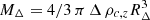 , where
  is the critical density of the universe at the observed redshift z of the cluster, G is the universal gravitational constant, and Hz = H0 [ΩΛ+Ωm(1+z)3]0.5 = H0 Ez is the value of the Hubble constant at the same redshift. For the ΛCDM model we adopt the cosmological parameters H0 = 70 km s−1 Mpc−1 and Ωm = 1 − ΩΛ = 0.3.
Historically, the characteristic thermodynamic quantities within a given overdensity Δ refer to a singular isothermal sphere with mass MΔ and radius RΔ in hydrostatic equilibrium. In this case mass and gas temperature are simply related by the equation (e.g. Voit et al. 2005)
 (1)
(1)
where μ is the mean molecular weight of the gas, ma is the atomic mass unit of 1.66 × 10⁻²⁴ g, and kB is the Boltzmann constant. Associating a mean electron density  , where fgas = Mgas(< RΔ)/MΔ is the mass gas fraction,
  is the mean gas density, and μ/μe = 0.52, with μe = 1.17 and μ = 0.61 being respectively the mean molecular weight of electrons and of the gas for a plasma with 0.3 solar abundance tabulated in Anders & Grevesse (1989)1, we can also write the mean values for pressure,
  , and for entropy,
  . Some characteristic values of these mean physical scales are quoted in Table 1 with their dependences on mass, redshift, and gas mass fraction.
Characteristic physical scales at two typical overdensities (Δ = 500 and 200 times the critical density at redshift z) for an input mass of 1015 M⊙, a gas mass fraction fgas = 0.1, and redshift 0.
2. Universal thermodynamic radial profiles
In this section we define the functional forms of the thermodynamic profiles for the ICM that will be integrated to recover the global properties to be compared with the corresponding quantities measured in X-ray observations. To define these functional forms, we assume an ICM in hydrostatic equilibrium within a spherically symmetric dark matter potential. Two simple ingredients are needed: a radial distribution for the mass, and a radial profile for one of the thermodynamic quantities (gas density, temperature, pressure, or entropy).
2.1. The semi-analytic model
To model the mass distribution we adopt a halo concentration–mass–redshift relation, c–M–z, for mass concentration c200, global mass value  , and redshift of the observed object for a Navarro-Frenk-White (NFW) mass density profile (Navarro et al. 1997) with concentration and radius at Δ = 200 related through the scale radius rs: c200 = R200/rs. We consider the c–M–z relation described in Dutton & Macciò (2014) (hereafter D14), with
  , B = −0.101 + 0.026z, and A = 0.520 + (0.905 − 0.520)exp(−0.617z1.21). We also use an alternative relation following the prescriptions described in Bhattacharya et al. (2013) (hereafter B13), which provides lower values of concentration by ∼10% (20%) at z ∼ 0.05 (1) in the mass range considered in the present study (1014 − 1015 M⊙; see also Diemer & Kravtsov 2015, for a detailed comparison between different models as a function of mass and redshift). We note that the quoted relations depend on the assumed cosmological parameters, but less significantly at M > 1014 M⊙, where the differences in predicted concentrations are on the order of a few per cent for the values of H0 and Ωm adopted here (see e.g. Fig. 9 in D14). We also note that the quoted c–M–z relations refer to the results extracted from dark matter only simulations. It is known that the distribution of baryons in the cluster halo can affect how concentration and total mass relate, causing for instance a steepening of the relation because star formation is fractionally more efficient in low-mass objects, with an overall larger normalisation because this effect is non-vanishing at all masses (see e.g. Fedeli 2012). However, it has been proved that, once a proper selection of N-body simulated systems is done to mimic an observational sample, the predicted c–M–z relation matches the observed one at least for very massive objects (at the 90% confidence level in the CLASH sample, where the total masses were recovered from the gravitational lensing signal; see Merten et al. 2015). Furthermore, considering that the adopted c–M–z relations were also used to infer the total masses in the Early Sunyaev-Zeldovich (ESZ) sample that will be analysed in our work, and that introducing the self-gravity due to the gas (the dominant baryonic component, although accounting for less than 15% of the total mass) would complicate, without much benefit, the calculations presented below, we use the quoted c–M–z relations as input to define the total mass of our systems.
It is worth noting that we are interested here in the global average behaviour of the cluster properties, and do not propagate any error and/or scatter on the mean quantities. The c–M–z relation is known to have an intrinsic scatter of σ log c ∼ 0.16 on the predicted values of the concentration for given mass (e.g. Diemer & Kravtsov 2015) that might be propagated through the relations used in this work to evaluate its impact on the reconstructed distribution of the observed thermodynamic profiles and integrated quantities of the ICM. We postpone to a future work further discussion on the distribution of the input parameters, although we also consider a different set of parameters (both for the c–M–z relation and for the pressure profile) depending on the dynamical state of the systems, such as relaxed cooling core objects that are expected to have higher halo concentration and higher values of pressure in the core (see Sect. 4).
The predictions on the radial behaviour of the interesting physical quantities are then recovered from the inversion of the hydrostatic equilibrium equation (see e.g. Ettori et al. 2013)
 (2)
(2)
where Pe = neTgas in units of keV cm−3 is described by a generalised NFW (e.g. Nagai et al. 2007; Arnaud et al. 2010)
![Mathematical equation: $$ \begin{aligned}&P_{e} = P_{500} \, E_z^{8/3} \, \left( \frac{M_{500}}{3 \times 10^{14} h_{70}^{-1} \,M_{\odot }} \right)^{\alpha _M} h_{70}^2 \, P_r \nonumber \\&P_r = \frac{P_0}{(c_{500} x)^{\Gamma }\, \left[1 + (c_{500} x)^A \right]^{(B- \Gamma ) / A}} \end{aligned} $$](/articles/aa/full_html/2020/12/aa38586-20/aa38586-20-eq20.gif) (3)
(3)
with x = r/R500, the normalisation  keV cm−32, the parameters (P0, c500, Γ, A, B) equal to (6.41, 1.81, 0.31, 1.33, 4.13), and αM = 0.12, accounting for the observed deviation from the standard self-similar scaling, set as in Planck Collaboration Int. V (2013). We have also considered an alternative pressure profile from the recent analysis of the joint XMM-Newton and Planck signals of a sample of 12 nearby massive galaxy clusters presented in Ghirardini et al. (2019). Converting the published values to feed Eq. (3), we set (P0, c500, Γ, A, B)) = (5.29, 1.49, 0.43, 1.33, 4.40) and αM = 0.
The total mass Mtot is defined equal to MHE/(1 − b), where Mtot is modelled with a NFW profile with parameters set according to the model adopted, and where the factor (1 − b) represents the hydrostatic bias that could affect the estimate of the hydrostatic masses MHE. We note that the hydrostatic bias is propagated to the shape of the gravitating mass profile through the halo concentration, whereas the input value MHE is adopted to define M500, used for instance to estimate P500 and R500. Following this procedure, we mimic the observational bias induced from the (biased) measurement of the mass on the normalising factor P500 and on the definition of the region over which the physical quantities are integrated. Instead, other quantities that are not directly used in the analysis (e.g. T500) are still defined from the bias-corrected Mtot.
We show in Fig. 1 the recovered profiles following these simple prescriptions. We present a few cases of interest, normalised to their average quantity at R500: a massive halo of 8 × 10¹⁴ M⊙ at redshift 0.05, which will be used as reference; the same halo with a different input pressure profile and mass bias of 0.4; a system with 1/4 of the mass at z = 0.05 and 1. While the assumption of the pressure profile has a negligible impact, in particular at r > 0.1 R500, large deviations (on the order of ∼20%) are induced by the mass (on all the profiles) and by the bias (on the temperature and density profile and, as a cumulative effect, on the entropy profile). The redshift causes measurable discrepancies, but lower than ∼20%.
 |
Fig. 1. Reconstructed thermodynamic radial profiles for objects with (M500, z) = (8 × 10¹⁴ M⊙, 0.05), black solid line; the same, but using a pressure profile from X-COP, red solid line, the B13 c − M − z relation, purple solid line; or assuming a hydrostatic bias b = 0.4, blue solid line; (M500, z) = (2 × 10¹⁴ M⊙, 0.05), black dashed line; (2 × 10¹⁴ M⊙, 1), red dashed line. The ratio is shown with respect to the reference case, black solid line, M500 = 8 × 10¹⁴ M⊙ and z = 0.05. P500, n500, T500, K500 refer to the normalisation values presented in Table 1. |
2.2. ESZ sample
To test and validate the predictions of our model, we use the radial profiles and the integrated quantities obtained for the ESZ sample (Lovisari et al. 2017, 2020), which contains the 120 galaxy clusters in the redshift range of 0.059 < z < 0.546 observed with XMM-Newton and which were originally selected from the Planck Early Sunyaev-Zeldovich (ESZ; Planck Collaboration VIII 2011) sample. As described in Lovisari et al. (2017), these systems, which have mass and redshift distributions representing well the whole ESZ sample of 188 galaxy clusters, are the ones for which R500 is completely covered by XMM-Newton observations.
As described in Lovisari et al. (2020), the radial temperature profiles were derived by requiring a S/N > 50 to ensure an uncertainty of ∼10% in the spectrally resolved temperature and a source-to-background count rate ratio higher than 0.6 to reduce the systematic uncertainties in their measurements. On average, the temperature profiles are extracted up to ∼R500.
The gas density profiles are presented in Lovisari et al. (2017). They are recovered as the geometrical deprojection of the best-fit results with a double-β model of the surface brightness profile extracted from the background-subtracted vignetting-corrected image in the 0.3–2 keV band defined to maximise the signal-to-noise ratio.
We present in Fig. 2 the comparison between the observed gas density and temperature profiles with those predicted from our model for a mass and redshift equal to the median values in the sample (M500 = 5.9 × 10¹⁴ M⊙, z = 0.193). Both the gas density and temperature profiles predicted from the model, the latter in particular at r > 0.3 R500, lie comfortably around the mean, and well within the scatter, of the observed values.
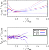 |
Fig. 2. Comparisons between the stacked profiles from the 120 objects analysed for the ESZ sample in Lovisari et al. (2020) and predictions from different models of (i) the universal pressure profile (Planck, used as reference, and X-COP) and (ii) the c − M − z relation (D14, used as reference, and B13) estimated at the median values in the sample of M500 and redshift. Top panel: electron density profiles recovered from the best-fit parameters of a double-β model. The solid line indicates the median value at each radius; the dotted lines show the 16th and 84th percentile estimated at each radius. The dashed line represents the extrapolation beyond the observational limit for the sample. Bottom panel: stacked temperature profile obtained from the weighted mean of 30 spectral points in each bin. Errors on the mean and dispersion (dotted lines) are overplotted. |
3. Integrated quantities
Using the thermodynamic profiles described in the previous section, we can reconstruct other derived profiles (e.g. the gas mass and the hydrostatic mass) and the integrated quantities (e.g. global temperature and luminosity).
The self-similar scenario predicts properties of the ICM that depend on the mass (and redshift) of the halo (see e.g. Voit 2005). In Ettori (2013, 2015) (hereafter E15) we describe the standard self-similar scenario and its possible deviations in terms of physical quantities depending explicitly on the mass. However, the reconstruction of the total mass in clusters is still affected by uncertainties (see e.g. Pratt et al. 2019) that make its use as a variable of reference a possible source of systematic errors. Therefore, in this study we prefer to write the scaling relations with respect to the observed temperature Tspec, which is a direct X-ray observable, also independent from cosmology. For our analysis, Tspec is the gas temperature measured as an integrated spectrum in the radial range 0.15 − 1 R500, and estimated from the profiles derived from our model as a “spectroscopic-like” value (see Mazzotta et al. 2004):
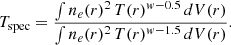 (4)
(4)
Here w = 0.75, T(r) = Pe(r)/ne(r), and the integrals are performed over the volume V(r) of interest, either up to R500 or between 0.15 and 1 R500.
The X-ray luminosity is obtained for a given gas density and temperature profile, assuming an apec model in XSPEC with a metallicity fixed to 0.3 times the solar values in Anders & Grevesse (1989) and integrating the emissivity in cylindrical volume extending up to 3 × R500 along the line of sight and covering an aperture between 0.15 and 1 R500.
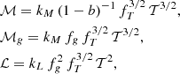
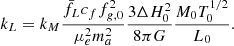
In the following we adopt the general description presented in E15. We define the total mass ℳ ≡ EzMtot/M0 (M0 = 5 × 10¹⁴ M⊙), the gas mass ℳg ≡ EzMg/Mg, 0 (Mg, 0 = 5 × 10¹³ M⊙), and a bolometric luminosity  (L0 = 5 × 1044 erg s−1). We write the normalisations and slopes of the scaling relations that relate these quantities to 𝒯 ≡ kBTspec/T0 (T0 = 5 keV) as
 (5)
(5)
where we have defined the following parameters: fT = T(R500)/T500 × T500/Tspec relates the gas temperature at R500 with the observed global value Tspec; the X-ray–measured gas mass fraction fg = Mg/MHE = (1 − b)−1Mg/Mtot = ≡C0.5 fnc/fg, 0 is normalised to fg, 0 = 0.1 and is related to the clumping-free gas mass fraction fnc through the clumping factor 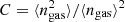 , defined as the ratio of the average squared gas density to the square of the mean gas density and that affects the measurement of the gas density as obtained from the deprojection of the X-ray free-free emission (e.g. Nagai & Lau 2011; Roncarelli et al. 2013; Vazza et al. 2013; Eckert et al. 2015); kM and kL (here referring to the case of a bolometric luminosity integrated over a spherical volume up to R500) are defined by constants (e.g. the overdensity Δ) and parameters that describe the shape of the thermodynamic profiles and are fully described in Appendix A. We note that the true gas mass fraction, i.e. the unbiased value from the hydrostatic bias and the clumping factor, is written in our notation as fgas = Mg/Mtot = (1 − b) fg = (1 − b) C0.5 fnc.
As extensively discussed in E15, any deviation from the standard self-similar behaviour can be ascribed to processes that impact the relative distribution of the gas and that, in the present study, we assume to be described as a power-law dependence on the gas temperature measured in the spectroscopic analysis 𝒯 ≡ kBTspec/5 keV:
 (6)
(6)
Here f0 is chosen to be 0.1 and is roughly representative of measured gas mass fractions, while t0 is set to  , the median value for our model as derived in Appendix A. We list these parameters, with their descriptions and definitions, in Table 2.
Descriptions and definitions of the parameters used in our model.
We insert them in Eq. (5) to write these equations in their full dependence on T as
 (7)
(7)
where we represent with N and S the best-fit estimates of normalisation and slope, respectively, of the corresponding scaling laws that are quoted in Table 3.
Then, by simple algebraic calculations, we can invert Eq. (7) and obtain the normalisations f0, t0, h0 and slopes f1, t1:
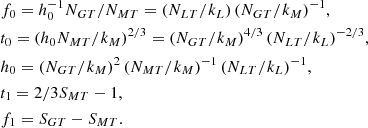 (8)
(8)
In Fig. 3, we show the reconstructed relations with the ICM temperature of the gas mass fraction, gas mass, and bolometric luminosity, and the corresponding best-fit relations that allow us to evaluate the normalisations N and slopes S. These values are then used to check the predicted behaviour of some intrinsic properties (e.g. the dependence on T of the gas mass fraction, and of the ratio T(R500)/T; see panels at the bottom of Fig. 3).
 |
Fig. 3. Top panels: global properties (empty black dots) and after correction for the Ez factor (solid red dots) recovered from their thermodynamic profiles for the following input values for (M500, z): (8 × 10¹⁴ M⊙, 0.05), (5 × 10¹⁴ M⊙, 0.05), (2 × 10¹⁴ M⊙, 0.05), (8 × 10¹⁴ M⊙, 0.5), (5 × 10¹⁴ M⊙, 0.5), (2 × 10¹⁴ M⊙, 1). The dashed magenta lines identify the best-fit relations of Eq. (7). A core-excised bolometric luminosity is considered. Bottom panels: red dots are the quantities (from left to right: fg, fT, b) estimated in our model for the following input values for (M500, z): (8 × 10¹⁴ M⊙, 0.05), (5 × 10¹⁴ M⊙, 0.05), (2 × 10¹⁴ M⊙, 0.05), (8 × 10¹⁴ M⊙, 0.5), (5 × 10¹⁴ M⊙, 0.5), and (2 × 10¹⁴ M⊙, 1); the blue dotted line indicates Ωb/Ωm = 0.157 (Planck Collaboration XXVII 2016); the dashed magenta lines show the predictions following the relations: fg = 0.124 𝒯0.23, fT = 0.687 𝒯0.07 and 1 − b = h0 = 1, where fg and fT are the absolute values, i.e. multiplied by the assumed normalisations of 0.1 and |

It is worth noting that, in order to compare our predictions with robust estimates of the X-ray luminosity, we integrate the bolometric luminosity within the radial range 0.15 − 1 R500, using quantities projected along the line of sight to mimic the observational values. These characteristics of the luminosity L (i.e. if projected or integrated over spherical shells, the radial range of integration, the energy band) define the proper value of the constant kL. Given the constraints on the L − T relation, we can invert it to recover kL under the assumption that there is no hydrostatic bias (i.e. (1 − b) = h0 = 1), so that t0 = (NMT/kM)2/3, f0 = NGT/NMT, and 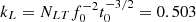 . We adopt this value of kL in the following analysis.
3.1. Calibration of the model in E15
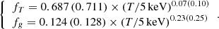
Our semi-analytic model makes use only of a universal pressure profile and a c–M–z relation, under the assumption that the total mass profile is described by a NFW model. The integrated quantities predicted from this model are used to calibrate the relations presented in E15 and described by Eqs. (5)–(8). By fitting in a robust way the distribution of points plotted in Fig. 3 when b is assumed to be zero, we obtain from Eq. (8) that these integrated quantities relate between them following the scaling laws built from self-similar relations and modified by including the following dependence of the temperature profile fT and of the gas mass fraction fg = C0.5fnc on Tspec, 0.15 − 1 R500:
 (9)
(9)
Here we quote in parentheses the results obtained by assuming a B13 model (where D14 is our model of reference) for the c–M–z relation.
3.2. Role of the hydrostatic bias
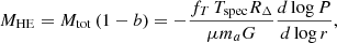
As described above, the hydrostatic bias is propagated to the total mass as Mtot = MHE/(1 − b), where Mtot is modelled with the adopted NFW profile, and the hydrostatic bias modifies the shape of the gravitating mass profile through the halo concentration. This affects all the thermodynamic quantities depending on the dark matter distribution, (e.g. T500) that is defined from the bias-corrected Mtot. On the other hand, the input value MHE is used to rescale the observed properties (e.g. R500 and P500) to mimic the observational bias once a biased MHE is measured instead of the true value Mtot.
In Fig. 4, we represent the impact of the hydrostatic bias as the ratio between quantities estimated with a given b value and with b = 0. A clear trend is present, with higher biases producing higher global temperatures, and lower estimates of Mg and L, mostly as consequence of the increased halo mass, associated with the corresponding reduction in the halo concentration and constant value of R500. We have also modelled the trend we observe in the physical quantities as a function of the assumed bias b with a functional form
 (10)
(10)
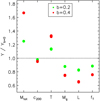 |
Fig. 4. Impact of the hydrostatic bias b on the integrated quantities, represented as the ratio between the quantities estimated for an assigned bias, and with bias equal to zero. From left to right: this ratio for total mass, temperature, gas mass, core-excised bolometric luminosity, and fT = T(R500)/Tspec. Shown is the case of a system with M500 = 5 × 10¹⁴ M⊙ at z = 0.05 and 0.5 (the values at different redshifts overlap for most of the quantities). |
such that when Y = Mtot, then (α0, α1) = (0, −1). For a typical object with M500 = 5 × 10¹⁴ M⊙ at z = 0.05 shown in Fig. 4, this functional form reproduces the observed trends within 2% and provides the following best-fit parameters (α0, α1): ( − 0.12, −0.45) for Tspec; (0.34, 0.39) for the gas mass; (0.83, 0.25) for the bolometric luminosity; (0.012, 2.61) for the gas fraction. Very similar results are obtained for systems at lower masses and higher redshifts on Tspec, Mg, and gas mass fraction.
This translates into the following representation in the E15 formalism for the two cases b = 0.2 and b = 0.4 (the latter in brackets), assuming the same set of input values of (M500, z)
 (11)
(11)
with lower normalisations for fg and fT for higher values of b, and no significant change in the dependence on the temperature.
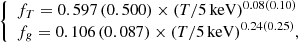
3.3. Results on the ESZ sample
Lovisari et al. (2020) present a study of the X-ray scaling relations for the ESZ sample, based on hydrostatic mass profiles recovered from the B13 c–M–z relation, and using core-excised luminosities and spectroscopic temperatures, as we reproduce in our semi-analytic model. The best-fit relations for the observational data are corrected for the Eddington bias, but not for the Malmquist bias, which is negligible when fitting the X-ray properties of an SZ selected sample (for more details, see Lovisari et al. 2020). The slopes of all the investigated scaling relations are found to deviate significantly from the self-similar predictions, if self-similar redshift evolution is assumed. We re-estimated normalisations and slopes of the scaling relations of interest using the package LIRA (Sereno 2016; see Table 3). In Fig. 5, we overplot these best-fit relations to the data points in the ESZ sample.
 |
Fig. 5. Distribution of the observed values for the ESZ sample with best-fit results from a linear fit in the logarithmic space (using LIRA; Sereno 2016). Predictions from the semi-analytic model (best-fit values in Table 3) are overplotted with dashed lines in magenta (for the D14 c − M − z relation) and blue (B13). Bottom panels: dashed lines indicate the ratios of the model (M) to the observed (O) best-fit relations. |
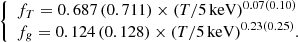
By applying our universal model, we require the self-similar predictions to be corrected by the following dependences on the gas temperature
 (12)
(12)
Here we propagate the errors on the best-fit parameters, and (as in the following analysis) we quote the absolute values of fg and fT, i.e. multiplied by their normalisation values of fg, 0 = 0.1 and  .
.
Then we compare the observed distribution with the predictions from our semi-analytic model. To mimic the distribution in mass and redshift of the ESZ sample, we simulated ten objects with our semi-analytic code having mass and redshift equal to the median values estimated in bins of 12 clusters each, sorted in redshift. We overplot these predictions to the data points in Fig. 5. We also use a different c–M–z relation to probe the dependence on the assumed model. As previously discussed, the B13 model predicts lower c200 at higher redshift, for a fixed halo mass. This behaviour induces differences in the estimates of T, L, and gas mass. For example, a halo with M500 = 5 × 10¹⁴ M⊙ is expected to have c200 lower by 5% and 13% at z = 0.05 and 0.5 in B13, inducing a slightly different distribution of the dark matter and consequent reshaping of the thermodynamic profiles that produce T lower by 2% and 4%, Mg higher by 2% and 4% and L higher by 3% and 9%, respectively.
The normalisations are within the 1σ intervals of the observational constraints (the largest tension being the results on NLT from the D14 model), whereas the slopes of the scaling laws in the ESZ sample tend to be systematically higher than the predicted values by 0.7–1.2σ, 2.6–2.1σ, and 3–2.4σ for the M − T, Mg − T, and L − T relation with D14 and B13 models, respectively. It is important to note, however, that the steepening of the relations might depend on the selection applied and on how the fit is performed (in our case, we consider in LIRA the scatter on both the variables X and Y, i.e. we leave the parameters sigma.XIZ.0 and sigma.YIZ.0 free to vary; for details, see Sereno 2016). For instance, if we fix sigma.XIZ.0 = 0, then the relations become flatter, with slopes of 1.60, 2.00, and 2.82 for the M − T, Mg − T, and L − T relation, respectively. In general, we obtain a better agreement between the observed distributions in the ESZ sample and the simulated data when we apply the B13 model as a consequence of the shift to lower temperatures for a given mass, and conclude that the distribution of the integrated physical quantities follows what is reconstructed from the universal model within 10%, on average.
Using Eq. (8) on these simulated data, and assuming a D14 model, the best-fit values convert into (t0, t1) = (0.689, 0.07); (f0, f1) = (0.122, 0.22) for h0 free to vary (best-fit: 1.02) and (t0, t1) = (0.680, 0.07); (f0, f1) = (0.124, 0.22) for h0 fixed to one. When B13 is adopted we obtain h0 = 1.01 once it is left to vary, (t0, t1) = (0.698, 0.10); (f0, f1) = (0.125, 0.25), and (t0, t1) = (0.694, 0.10); (f0, f1) = (0.126, 0.25) with h0 fixed to one. Overall, there is a good consistency with the results shown in Eq. (12), apart from a clear steeper dependence of the gas fraction on T that will be discussed further in the next subsection.
3.4. Including the distribution of YSZ
The same plasma responsible for the X-ray emission can also be traced through the Sunyaev-Zeldovich (SZ) effect, generated from the Compton scattering of the photons of the cosmic microwave background on the electrons of the ICM (Sunyaev & Zeldovich 1972). The millimetre wave emission due to the thermal SZ effect is proportional to the integrated pressure of the X-ray emitting plasma along the line of sight and is described, as aperture integrated signal (see e.g. Mroczkowski et al. 2019), by the integrated Compton parameter 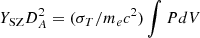 , where DA is the angular diameter distance to the cluster, σT = 8π/3(e2/mec2)2 = 6.65 × 10⁻²⁵ cm2 is the Thomson cross section, me and e are respectively the electron rest mass and charge, c is the speed of light, and P = neT is the electron pressure profile.
Using the formalism presented in E15, this signal relates to the gas temperature as
 (13)
(13)
where kSZ is derived in Appendix B.
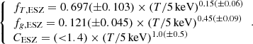
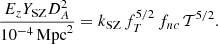
It is worth noting a few issues concerning the reconstruction of the SZ signal. First, the SZ signal depends linearly on the pressure profile and is sensitive to the upper limit of the integration. We collect the estimates of the spherically integrated SZ flux up to R500YSZ from the PSZ1 catalogue3 (Planck Collaboration XIV 2015). We refer to Planck Collaboration XIII (2016) for an exhaustive discussion on how YSZ is recovered from the integrated Comptonisation Y5 R500, which represents a nearly unbiased proxy for the total SZ flux within a cylinder of aperture radius 5 R500 and needs to be corrected for the degeneracy induced from the signal-size correlation and underlying variations of the pressure profile of reference inducing extra scatter and bias in the extrapolation (see Sects. 5.1–5.3 and Fig. 16 in Planck Collaboration XIII 2016).
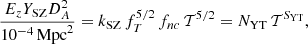
A second issue is that the gas fraction fnc in Eq. (13) refers to the clumping-free value, i.e. a gas mass fraction that does not depend on the gas clumping described by the factor C that appears in Eq. (5) above. By combining now the scaling relations based on SZ data and those using X-ray quantities, and modelling the gas clumping as C = C0 𝒯C1, we can write  , where fnc, 0 and fnc, 1 indicate the normalisation and slope, respectively, of the gas fraction after the correction for the clumping. After simple calculations we obtain
 (14)
(14)
and proceed with the estimates of the gas clumping and the corrected gas fraction using the values of fT and fg quoted in Eqs. (9) and (12).
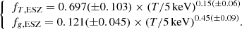
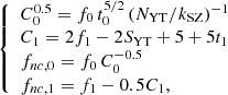
We present the results of our analysis in Fig. 6. By fitting a linear relation in the log space on the sample of ten objects simulated with our semi-analytic model to mimic the observed distribution in mass and redshift of the ESZ sample, we measure (NYT, SYT) = (0.33, 2.84) when a D14 c–M–z relation is assumed, and (0.35, 2.92) for the B13 relation. Using the relations imposed by our universal model (see Eq. (14)), we constrain the gas clumping to be (C0, C1) = (1.00, 0.12) and (1.04, 0.17) for the D14 and B13 model, respectively. Considering that our model does not include any gas clumping, we can consider these values as indicators of the systematic uncertainties (on the order of a few per cent) that affect our reconstruction of the ICM properties.
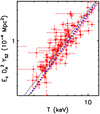 |
Fig. 6. YSZ − T relation for the ESZ sample with the best-fit results from a linear fit in the logarithmic space. The fit on the observed data is performed using LIRA (black dotted line). The predictions from the semi-analytic model overlap (magenta dashed line: D14 model; blue dashed line: B13 model). The dot-dashed orange line is obtained from the propagation of the scaling in the E15 formalism (see Eq. (13)). |
When the same analysis is applied to the ESZ sample, we estimate (NYT, SYT) = (0.42 ± 0.03, 2.79 ± 0.18). These results are consistent with the best-fit constraints obtained for 62 objects listed in a Planck Early Results work (Planck Collaboration XI 2011, redoing the fit, we measure a normalisation in the adopted units of 0.37 ± 0.01 and slope of 2.97 ± 0.18). Adopting as reference the best-fit values for the ESZ sample, we investigate how we can reconcile the observed differences with our predictions. We note that the normalisation NYT depends on the gas fraction and fT. As discussed in Sect. 3.2, any hydrostatic bias induces lower values of fg and fT, decreasing the normalisation and enlarging the tension with the observed constraints. By combining the constraints on fg and fT with the relations in Eq. (14), we conclude that the ESZ dataset is consistent with a gas clumping C0 < 1.4 (at the 1σ confidence level), in close agreement with the expected values within R500 from hydrodynamical simulations (see e.g. Nagai & Lau 2011; Roncarelli et al. 2013; Vazza et al. 2013; Eckert et al. 2015). From the best-fit results, we can also constrain C1 ∼ 1.0(±0.5), which represents a further contribution to the dependence on T of the gas fraction, explaining the steeper dependence quoted in Eq. (12) with respect to the predictions from the model.
4. Discussion
Our model combines a universal profile for the gas pressure with the present knowledge on the distribution of the dark matter in galaxy clusters to calibrate properly any deviations from the standard self-similar scenario. In particular, three quantities are introduced to account for these deviations: a temperature-dependent gas mass fraction, fg; a temperature-dependent ratio between the temperature at given radius and its global value, fT; a hydrostatic bias, b. To explain self-consistently the scaling relations observed in our model and those recovered in the ESZ sample, we require a significant dependence on T of the gas fraction, and a milder dependence of fT.
As numerical simulations suggest, and also analyses of the observed gas density distribution as a function of the measured temperature, more massive (hotter) systems tend to have a relatively higher gas density in the cores than groups (see e.g. Croston et al. 2008; Eckert et al. 2016), where feedback from central AGNs can efficiently contrast the attraction from gravity and push gas particles beyond R500. The net effect is a reduction of the gas mass fraction in objects at lower masses. This variation of the gas mass fraction with the gas temperature (or total mass) is well documented in past works, mostly based on X-ray selected samples (e.g. Pratt et al. 2009; Eckert et al. 2013, 2016; Lovisari et al. 2015; Ettori 2015), with constraints on normalisations and slopes that are quite similar, but not identical, to the values we obtain in our study and summarise in Eq. (12). For example, by converting to our units, Pratt et al. (2009) estimate fg = 0.107 × (T/5 keV)0.36; Lovisari et al. (2015) measure fg = 0.106 × (T/5 keV)0.32; Ettori (2015) obtains fg = 0.107 × (T/5 keV)0.33; and Eckert et al. (2016) obtain fg = 0.079 × (T/5 keV)0.35, which is on the lower side probably due to a bias in the weak-lensing mass measurements (see e.g. Umetsu et al. 2020). Using the estimates within R500 of the gas mass, total mass, and temperature obtained for the ESZ sample, we can directly fit the gas fraction–temperature relation and obtain fg = 0.123(±0.002) × (T/5 keV)0.39(±0.05), in agreement with our indirect calculations. However, these values of the gas fraction at a given temperature are 15-20% higher than those from the literature cited above. As discussed in Lovisari et al. (2020), part of this offset can be attributed to the nature of the ESZ sample, containing a larger number of disturbed clusters for which higher gas fractions are measured (see also Eckert et al. 2013) as a cumulative effect of gas clumpiness and inhomogeneities (inducing higher gas mass), larger non-thermal contribution to the total pressure (biasing low the total mass), and possible violation of the hydrostatic equilibrium. It is indeed known that SZ selected samples tend to have a larger contribution of dynamically disturbed clusters than X-ray selected ones, as also confirmed for the ESZ sample (see e.g. Lovisari et al. 2017).
We can evaluate the impact of having more relaxed objects on our relations. We repeat the analysis by assuming a pressure profile for cool-core systems, with (P0, c500, Γ, A, B) = (11.82, 0.60, 0.31, 0.76, 6.58) (see Planck Collaboration Int. V 2013), and using the c–M–z relation for relaxed systems in Bhattacharya et al. (2013). Still assuming no hydrostatic bias (b = 0), higher mass concentrations associated with relaxed objects produce higher normalisations of fg by 5–10%. To compensate for this rise affecting more X-ray selected samples, and to further reduce their estimates of fg, we are forced to require the presence of a hydrostatic bias of about 0.2. As we discuss in Sect. 3.2, the presence of any hydrostatic bias propagates to all the derived quantities, lowering fg for a given initial set of (M500, z). A bias of 0.2 causes a reduction of 15% or more in the normalisation of fg, allowing us, by compensating for the increase due to a larger contribution of relaxed clusters, to match the published results based on X-ray selected samples. A similar (or even higher) bias should also be present in the ESZ sample due to the larger contribution of disturbed systems. The presence of more disturbed systems should induce larger inhomogeneities in the gas distribution, which would bias high the reconstructed gas density and the corresponding gas mass fraction (e.g. Roncarelli et al. 2013), so that any correction for it would move fg to lower values.
On the other hand, the results on fg in the ESZ sample matches the predictions of our semi-analytic model with b = 0. It is worth noting that the adopted input models describe the ESZ sample best because we consider the average pressure profile recovered for Planck selected systems and use the c–M–z relation estimated for the entire collection of haloes (i.e. also including more disturbed systems). So, it seems that a sort of conspiracy acts to mimic fg with b = 0, although we are fairly confident that the ESZ sample contains a larger number of disturbed objects than in X-ray selected samples.
As we discuss in Sect. 3.2, the hydrostatic bias impacts all the integrated quantities. We evaluate how it affects the normalisation of fg (see also Eq. (11)), and model it as
 (15)
(15)
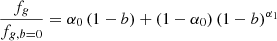
with (α0, α1) = (0.48, 0.44). Assuming that  is the observed value including the gas clumping, and fg, b = 0 = 0.124 (0.126) is set from our models (see end of Sect. 3.3), by adopting the upper limit on the gas clumping obtained from the YSZ − T relation (see Sect. 3.4), we conclude that the level of hydrostatic bias allowed in the ESZ sample has to be below 0.24 (0.26) at the 1σ level for the D14 (B13) model (see Fig. 7).
 |
Fig. 7. Dependence of the normalisation of fg upon the bias b (red line; see Eq. (15)). The shaded region (and the region between dashed lines) represents the quantity fnc/fg, b = 0, where |

The evidence that the ESZ sample includes disturbed systems might then account for the measured fg by a combination of the presence of hydrostatic bias (b > 0) and gas clumping (C > 1) induced by large gas inhomogeneities.
The other quantity we introduced, fT = T(R500)/T500 × T500/Tspec = T(R500)/Tspec, has never been investigated before and comes from our request to build a proper normalisation for the M − T relation, where the hydrostatic mass depends on the measurement of the temperature at a given radius (T(R500)). As we show in Fig. 3, fT is expected to increase mildly in the hotter systems, with a global effect that might account for some of the deviations observed in the standard self-similar scenario. Moreover, the normalisation decreases with increasing hydrostatic bias b (see Fig. A.1).
5. Conclusions
The gravitational force aggregates matter onto galaxy clusters, driving them to the virialisation and regulating the distribution and the energetic budget of the accreted baryons and the emergent observational properties of the ICM. We show how a universal pressure profile of the ICM, combined with a halo mass – concentration – redshift relation (either the model in D14 or in B13) and the hydrostatic equilibrium equation, allows the radial profiles of the thermodynamic quantities to be reconstructed. Once integrated over some typical scale (e.g. R500), these quantities produces observables (such as gas mass, temperature, luminosity, total mass, and SZ Compton parameter), which satisfy universal scaling laws that are the simple combination of self-similar relations, regulated from the mass and redshift of the halo, and further dependences of the gas temperature measured at the radius of reference, T(R500), and of the gas mass fraction, fg = C0.5fnc, on the observed spectroscopic measurement, Tspec, 0.15 − 1 R500.
We calibrated these dependences both within our framework and using one of the largest samples of X-ray luminous galaxy clusters that has been homogeneously analysed, the ESZ sample (Lovisari et al. 2017, 2020). We demonstrate that self-similar scaling laws hold between the integrated X-ray observables, once fT = T(R500)/T500 × T500/Tspec and fg = C0.5 fnc are allowed to depend on T ≡ Tspec as fT = t0𝒯t1 and fg = f0𝒯f1 (see also Table 2 for a description of these quantities) with the following constraints on the parameters obtained from our semi-analytic model (values for the B13 c–M–z relation in parentheses):
 (16)
(16)
In the ESZ sample, by propagating these dependences to the SZ signal, and interpreting any mismatch between the best-fit results of the observational data and the predictions from our semi-analytic and theoretical models as a measure of the gas clumping, we estimate
 (17)
(17)
This level of gas clumping within R500 is consistent with the value measured in hydrodynamical simulations, and supports the evidence that SZ selected samples, like the ESZ one, tend to have a representative contribution of dynamically disturbed clusters (see e.g. Lovisari et al. 2017) with a relative significant presence of gas inhomogeneities, in particular at large scales (see e.g. Roncarelli et al. 2013; Vazza et al. 2013). This upper limit on the gas clumping implies a level of hydrostatic bias b (see Eq. (15) and Fig. 7) below 25%, on average.
We conclude that our semi-analytic model reproduces well the observed properties of galaxy clusters, both resolved spatially and as integrated quantities. By providing the calibration of this physically motivated model in terms of the standard self-similar scaling relations, modified by three components that are able to account completely for the observed deviations, we can also deduce some other interesting properties.
For instance, these explicit forms of the dependences on the observed gas temperature allow us to modify accordingly the characteristic physical quantities that renormalises the observed profiles. In Table 4 we quote how the dependences implied by the universal model propagate and modify some of these quantities. For example, P500, which in a self-similar model scales as  , is expected to scale (in parentheses, the values for the B13 model) as T1.29(1.35) or
  , which is consistent with the rescaling of
 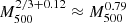 suggested in Arnaud et al. (2010) (and adopted in Planck Collaboration Int. V 2013).
Dependences of the characteristic physical scales on the temperature and mass in the universal model.
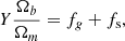
Moreover, we can write the baryonic depletion parameter Y with its explicit dependence on the gas temperature (or mass) as
 (18)
(18)
where fs represents the stellar mass fraction (∼0.015; see e.g. Eckert et al. 2019), and the ratio of the cosmic baryon density to matter density parameters, Ωb/Ωm, is equal to 0.157 (Planck Collaboration XXVII 2016). From the results of our semi-analytic model with a D14 (B13) c–M–z relation, we predict an average value of Y = 0.787(0.813) (T/5 keV)0.23(0.25) + 0.095.
In the same framework, we show that any calibration of the Mtot − T relation with mass measurements that do not rely on the hydrostatic equilibrium equation can be used to constrain the hydrostatic bias b, preserving the use of the self-similar relations in this case as well. On the other hand, by controlling the bias b we can make predictions on the expected variations in the observed properties and, for example, explain the published relations between gas mass fraction and temperature (see Sect. 4) by requiring a hydrostatic bias b ≳ 0.2, as illustrated in Sect. 3.2.
The application of this model to a accurately selected sample of a large number (∼100) of objects analysed homogeneously in their X-ray and lensing signal out to R500 and beyond as the one that will soon be available for the XMM-Newton Heritage Galaxy Cluster Project4 will allow us to extend the calibration and our understanding of the physical processes that regulate the interplay of baryons and dark matter in galaxy clusters.
Overall, our study demonstrates that the observed properties, both spatially resolved and integrated values, of X-ray luminous galaxy clusters are understood well. This represents a further step in the process to standardise their observables on the basis of a physically motivated model, not only to fully appreciate the phenomena that shape the distribution of baryons and regulate their energetic budget, but also to control biases that could affect their use as cosmological proxies.
μe = 1.16 and μ = 0.60 are also obtained for the popular abundance table adopted for the X-ray spectral analysis in Asplund et al. (2009).
For the sake of clarity, here (μ, μe, fg, 500) = (0.59, 1.14, 0.175) are assumed for consistency with the original work and the associated best-fit parameters; in the following analysis, we use the values of μ and μe quoted in Sect. 1.
We use the catalogue PSZ1v2.1.fits available, with description, at http://szcluster-db.ias.u-psud.fr/.
Differently from what we describe in Ettori (2015), here the logarithmic slope β of the pressure profile at R500 does not depend on the mass because the further exponent α1 is set to 0.
Acknowledgments
We thank the anonymous referee for insightful comments that helped in improving the presentation of the work. We acknowledge financial contribution from the contracts ASI-INAF Athena 2015-046-R.0, ASI-INAF Athena 2019-27-HH.0, “Attività di Studio per la comunità scientifica di Astrofisica delle Alte Energie e Fisica Astroparticellare” (Accordo Attuativo ASI-INAF n. 2017-14-H.0), and from INAF “Call per interventi aggiuntivi a sostegno della ricerca di main stream di INAF”. This research has made use of the SZ-Cluster Database operated by the Integrated Data and Operation Center (IDOC) at the Institut d’Astrophysique Spatiale (IAS) under contract with CNES and CNRS.
References
- Anders, E., & Grevesse, N. 1989, Geochim. Cosmochim. Acta, 53, 197 [Google Scholar]
- Arnaud, M., Pratt, G. W., Piffaretti, R., et al. 2010, A&A, 517, A92 [NASA ADS] [CrossRef] [EDP Sciences] [Google Scholar]
- Asplund, M., Grevesse, N., Sauval, A. J., & Scott, P. 2009, ARA&A, 47, 481 [NASA ADS] [CrossRef] [Google Scholar]
- Baldi, A., Ettori, S., Molendi, S., & Gastaldello, F. 2012, A&A, 545, A41 [NASA ADS] [CrossRef] [EDP Sciences] [Google Scholar]
- Bhattacharya, S., Habib, S., Heitmann, K., & Vikhlinin, A. 2013, ApJ, 766, 32 [NASA ADS] [CrossRef] [Google Scholar]
- Böhringer, H., Dolag, K., & Chon, G. 2012, A&A, 539, A120 [NASA ADS] [CrossRef] [EDP Sciences] [Google Scholar]
- Croston, J. H., Pratt, G. W., Böhringer, H., et al. 2008, A&A, 487, 431 [NASA ADS] [CrossRef] [EDP Sciences] [Google Scholar]
- Diemer, B., & Kravtsov, A. V. 2015, ApJ, 799, 108 [NASA ADS] [CrossRef] [Google Scholar]
- Dutton, A. A., & Macciò, A. V. 2014, MNRAS, 441, 3359 [Google Scholar]
- Eckert, D., Ettori, S., Molendi, S., Vazza, F., & Paltani, S. 2013, A&A, 551, A23 [NASA ADS] [CrossRef] [EDP Sciences] [Google Scholar]
- Eckert, D., Roncarelli, M., Ettori, S., et al. 2015, MNRAS, 447, 2198 [NASA ADS] [CrossRef] [Google Scholar]
- Eckert, D., Ettori, S., Coupon, J., et al. 2016, A&A, 592, A12 [NASA ADS] [CrossRef] [EDP Sciences] [Google Scholar]
- Eckert, D., Ghirardini, V., Ettori, S., et al. 2019, A&A, 621, A40 [NASA ADS] [CrossRef] [EDP Sciences] [Google Scholar]
- Ettori, S. 2013, MNRAS, 435, 1265 [NASA ADS] [CrossRef] [Google Scholar]
- Ettori, S. 2015, MNRAS, 446, 2629 [NASA ADS] [CrossRef] [Google Scholar]
- Ettori, S., Donnarumma, A., Pointecouteau, E., et al. 2013, Space Sci. Rev., 177, 119 [Google Scholar]
- Fedeli, C. 2012, MNRAS, 424, 1244 [NASA ADS] [CrossRef] [Google Scholar]
- Ghirardini, V., Eckert, D., Ettori, S., et al. 2019, A&A, 621, A41 [NASA ADS] [CrossRef] [EDP Sciences] [Google Scholar]
- Kaiser, N. 1986, MNRAS, 222, 323 [Google Scholar]
- Kravtsov, A. V., & Borgani, S. 2012, ARA&A, 50, 353 [NASA ADS] [CrossRef] [Google Scholar]
- Kravtsov, A. V., Vikhlinin, A., & Nagai, D. 2006, ApJ, 650, 128 [Google Scholar]
- Lovisari, L., Reiprich, T. H., & Schellenberger, G. 2015, A&A, 573, A118 [NASA ADS] [CrossRef] [EDP Sciences] [Google Scholar]
- Lovisari, L., Forman, W. R., Jones, C., et al. 2017, ApJ, 846, 51 [NASA ADS] [CrossRef] [Google Scholar]
- Lovisari, L., Schellenberger, G., Sereno, M., et al. 2020, ApJ, 892, 102 [CrossRef] [Google Scholar]
- Mazzotta, P., Rasia, E., Moscardini, L., & Tormen, G. 2004, MNRAS, 354, 10 [NASA ADS] [CrossRef] [Google Scholar]
- Merten, J., Meneghetti, M., Postman, M., et al. 2015, ApJ, 806, 4 [NASA ADS] [CrossRef] [Google Scholar]
- Mroczkowski, T., Nagai, D., Basu, K., et al. 2019, Space Sci. Rev., 215, 17 [NASA ADS] [CrossRef] [Google Scholar]
- Nagai, D., & Lau, E. T. 2011, ApJ, 731, L10 [NASA ADS] [CrossRef] [Google Scholar]
- Nagai, D., Kravtsov, A. V., & Vikhlinin, A. 2007, ApJ, 668, 1 [Google Scholar]
- Navarro, J. F., Frenk, C. S., & White, S. D. M. 1997, ApJ, 490, 493 [NASA ADS] [CrossRef] [Google Scholar]
- Planck Collaboration VIII. 2011, A&A, 536, A8 [NASA ADS] [CrossRef] [EDP Sciences] [Google Scholar]
- Planck Collaboration XI. 2011, A&A, 536, A11 [NASA ADS] [CrossRef] [EDP Sciences] [Google Scholar]
- Planck Collaboration XIV. 2015, A&A, 581, A14 [NASA ADS] [CrossRef] [EDP Sciences] [Google Scholar]
- Planck Collaboration XIII. 2016, A&A, 594, A13 [NASA ADS] [CrossRef] [EDP Sciences] [Google Scholar]
- Planck Collaboration XXVII. 2016, A&A, 594, A27 [NASA ADS] [CrossRef] [EDP Sciences] [Google Scholar]
- Planck Collaboration Int. V. 2013, A&A, 550, A131 [NASA ADS] [CrossRef] [EDP Sciences] [Google Scholar]
- Pratt, G. W., Croston, J. H., Arnaud, M., & Böhringer, H. 2009, A&A, 498, 361 [NASA ADS] [CrossRef] [EDP Sciences] [Google Scholar]
- Pratt, G. W., Arnaud, M., Piffaretti, R., et al. 2010, A&A, 511, A85 [NASA ADS] [CrossRef] [EDP Sciences] [Google Scholar]
- Pratt, G. W., Arnaud, M., Biviano, A., et al. 2019, Space Sci. Rev., 215, 25 [NASA ADS] [CrossRef] [Google Scholar]
- Roncarelli, M., Ettori, S., Borgani, S., et al. 2013, MNRAS, 432, 3030 [NASA ADS] [CrossRef] [Google Scholar]
- Sereno, M. 2016, MNRAS, 455, 2149 [NASA ADS] [CrossRef] [Google Scholar]
- Sunyaev, R. A., & Zeldovich, Y. B. 1972, Comm. Astrophys. Space Phys., 4, 173 [Google Scholar]
- Umetsu, K., Sereno, M., Lieu, M., et al. 2020, ApJ, 890, 148 [CrossRef] [Google Scholar]
- Vazza, F., Eckert, D., Simionescu, A., Brüggen, M., & Ettori, S. 2013, MNRAS, 429, 799 [NASA ADS] [CrossRef] [Google Scholar]
- Vikhlinin, A., Kravtsov, A., Forman, W., et al. 2006, ApJ, 640, 691 [NASA ADS] [CrossRef] [Google Scholar]
- Voit, G. M. 2005, Rev. Mod. Phys., 77, 207 [NASA ADS] [CrossRef] [Google Scholar]
- Voit, G. M., Kay, S. T., & Bryan, G. L. 2005, MNRAS, 364, 909 [NASA ADS] [CrossRef] [Google Scholar]
Appendix A: Derivations of kM and kL
In Eq. (5) we introduce some constants that appear in the normalisations of the scaling relations Mtot − T and L − T, namely kM and kL. We present here the steps that lead to their definitions.
The hydrostatic mass at the given overdensity Δ is defined as
 (A.1)
(A.1)
where we have defined the quantity fT = T(RΔ)/Tspec that relates the gas temperature at RΔ with the observed global value Tspec. By definition, the same mass is equal to 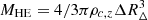 , where
  . By inverting the latter equation, we obtain
  that we use to replace RΔ in Eq. (A.1). After this substitution, we solve for Mtot and obtain
 (A.2)
(A.2)
where we define β as the logarithmic slope of the pressure profile at RΔ (β = −d log P/d log r5). Finally, collecting all the constants on the right side of the equation, and recalling that Hz = EzH0, we can write
 (A.3)
(A.3)
which allows us to define the constant kM as the normalisation of the relation
 (A.4)
(A.4)
where
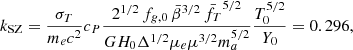
 (A.5)
(A.5)
Using Δ = 500 and the median values  (identical for all the systems being the same as the pressure profile adopted) and
  (with values in the range of −6%, +2% for b = 0; see Fig. A.1), and the adopted pivot values T0 and M0, we measure kM = 0.883.
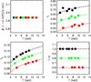 |
Fig. A.1. Distribution of the parameters β, fT, fg, and 1 − b as a function of T and colour-coded according to the assumed hydrostatic bias (black: b = 0; green: b = 0.2; red: b = 0.4). The dashed lines in the panel at the bottom right are recovered through the process described in Eq. (8). Points represent quantities derived for the following input values for (M500, z): (8 × 10¹⁴ M⊙, 0.05), (5 × 10¹⁴ M⊙, 0.05), (2 × 10¹⁴ M⊙, 0.05), (8 × 10¹⁴ M⊙, 0.5), (5 × 10¹⁴ M⊙, 0.5), with and without a bias b; a further case (2 × 10¹⁴ M⊙, 1) with b = 0 is considered. |
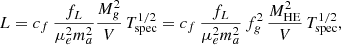
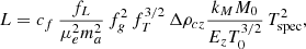
Consider now the L − T relation. By definition, the X-ray luminosity is equal to the integral over the volume V of interest of the X-ray emissivity ϵ = nenpΛ(T, Z):
 (A.6)
(A.6)
A selection of the X-ray band where the luminosity is measured will affect the estimate of the cooling function Λ(T, Z), which depends on the gas temperature and metallicity. For a bolometric luminosity we can write  , with cf = 1.02 × 10⁻²³ erg s−1 cm−3 (see discussion in Sect. 2 of E15), and write
 (A.7)
(A.7)
where we have defined 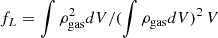 as the correction needed to consider the gas mass (Mg = ∫ρgasdV) instead of the emission integral (
 ), with ρgas = μemane, for scaling purposes. Here the integrals are performed over a spherical volume between 0 and R500. Using the above relation between total mass and temperature and total mass and volume, we can do the final step and write
 (A.8)
(A.8)
which can be expressed in the form
 (A.9)
(A.9)
with
 (A.10)
Using the median value of fL,  (with values in the range −8%, +2%), fg, 0 = 0.1, and the adopted values of Δ, T0, M0, and L0, we measure kL = 0.930.
Appendix B: Derivation of kSZ
In Eq. (13) we introduce the constant kSZ in the normalisation of the Y − T relation:
 (B.1)
(B.1)
Here fT and fg are the values normalised to the median value we observe in our model  (see Fig. A.1) and 0.1, respectively, and fnc is the clumping-free gas mass fraction that is related to the X-ray-measured quantity fg through the relation fg = C0.5 fnc, where
  is the clumping factor.
To define kSZ, we proceed from the definition of 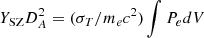 , where DA is the angular diameter distance to the cluster, σT = 8π/3(e2/mec2)2 = 6.65 × 10⁻²⁵ cm2 is the Thomson cross section, and ∫PedV = ∫neTdV ≈ fT Tspec MgC−0.5/(μema) = fg C−0.5 fT TspecMHE/(μema).
By substituting MHE from Eq. (A.4), we can write
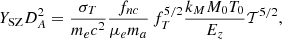 (B.2)
(B.2)
which allows us to define the constant
 (B.3)
(B.3)
where fg, 0 = 0.1,  ,
,  , T0 = 5 keV, Y0 = 10−4 Mpc2, and cP = ∫PedV × (μema)/(MgfTTspec) has a typical value of 1.36 (dimensionless) with variations of ±1% in the range of T and redshift studied here.
It should be noted that using YX = Mg × T, which is the X-ray analogue of the integrated Compton parameter introduced by Kravtsov et al. (2006), we can write cP = YSZ/(cXSZYXfT), where cXSZ = σT/(mec2 μema)≈1.40 × 10⁻¹⁹ Mpc2
 keV−1. Therefore, we predict a ratio C = YSZ/(cXSZYX) = cP fT equal to median values of 0.924 (with D14 model) and 0.927 (B13) with relative changes of ±1% in the redshift and mass ranges investigated in this paper, in close agreement with the present observational constraints (see e.g. Arnaud et al. 2010).
All Tables
Characteristic physical scales at two typical overdensities (Δ = 500 and 200 times the critical density at redshift z) for an input mass of 1015 M⊙, a gas mass fraction fgas = 0.1, and redshift 0.
Dependences of the characteristic physical scales on the temperature and mass in the universal model.
All Figures
|
Fig. 1. Reconstructed thermodynamic radial profiles for objects with (M500, z) = (8 × 10¹⁴ M⊙, 0.05), black solid line; the same, but using a pressure profile from X-COP, red solid line, the B13 c − M − z relation, purple solid line; or assuming a hydrostatic bias b = 0.4, blue solid line; (M500, z) = (2 × 10¹⁴ M⊙, 0.05), black dashed line; (2 × 10¹⁴ M⊙, 1), red dashed line. The ratio is shown with respect to the reference case, black solid line, M500 = 8 × 10¹⁴ M⊙ and z = 0.05. P500, n500, T500, K500 refer to the normalisation values presented in Table 1. |
| In the text | |
|
Fig. 2. Comparisons between the stacked profiles from the 120 objects analysed for the ESZ sample in Lovisari et al. (2020) and predictions from different models of (i) the universal pressure profile (Planck, used as reference, and X-COP) and (ii) the c − M − z relation (D14, used as reference, and B13) estimated at the median values in the sample of M500 and redshift. Top panel: electron density profiles recovered from the best-fit parameters of a double-β model. The solid line indicates the median value at each radius; the dotted lines show the 16th and 84th percentile estimated at each radius. The dashed line represents the extrapolation beyond the observational limit for the sample. Bottom panel: stacked temperature profile obtained from the weighted mean of 30 spectral points in each bin. Errors on the mean and dispersion (dotted lines) are overplotted. |
| In the text | |
|
Fig. 3. Top panels: global properties (empty black dots) and after correction for the Ez factor (solid red dots) recovered from their thermodynamic profiles for the following input values for (M500, z): (8 × 10¹⁴ M⊙, 0.05), (5 × 10¹⁴ M⊙, 0.05), (2 × 10¹⁴ M⊙, 0.05), (8 × 10¹⁴ M⊙, 0.5), (5 × 10¹⁴ M⊙, 0.5), (2 × 10¹⁴ M⊙, 1). The dashed magenta lines identify the best-fit relations of Eq. (7). A core-excised bolometric luminosity is considered. Bottom panels: red dots are the quantities (from left to right: fg, fT, b) estimated in our model for the following input values for (M500, z): (8 × 10¹⁴ M⊙, 0.05), (5 × 10¹⁴ M⊙, 0.05), (2 × 10¹⁴ M⊙, 0.05), (8 × 10¹⁴ M⊙, 0.5), (5 × 10¹⁴ M⊙, 0.5), and (2 × 10¹⁴ M⊙, 1); the blue dotted line indicates Ωb/Ωm = 0.157 (Planck Collaboration XXVII 2016); the dashed magenta lines show the predictions following the relations: fg = 0.124 𝒯0.23, fT = 0.687 𝒯0.07 and 1 − b = h0 = 1, where fg and fT are the absolute values, i.e. multiplied by the assumed normalisations of 0.1 and |
| In the text | |
|
Fig. 4. Impact of the hydrostatic bias b on the integrated quantities, represented as the ratio between the quantities estimated for an assigned bias, and with bias equal to zero. From left to right: this ratio for total mass, temperature, gas mass, core-excised bolometric luminosity, and fT = T(R500)/Tspec. Shown is the case of a system with M500 = 5 × 10¹⁴ M⊙ at z = 0.05 and 0.5 (the values at different redshifts overlap for most of the quantities). |
| In the text | |
|
Fig. 5. Distribution of the observed values for the ESZ sample with best-fit results from a linear fit in the logarithmic space (using LIRA; Sereno 2016). Predictions from the semi-analytic model (best-fit values in Table 3) are overplotted with dashed lines in magenta (for the D14 c − M − z relation) and blue (B13). Bottom panels: dashed lines indicate the ratios of the model (M) to the observed (O) best-fit relations. |
| In the text | |
|
Fig. 6. YSZ − T relation for the ESZ sample with the best-fit results from a linear fit in the logarithmic space. The fit on the observed data is performed using LIRA (black dotted line). The predictions from the semi-analytic model overlap (magenta dashed line: D14 model; blue dashed line: B13 model). The dot-dashed orange line is obtained from the propagation of the scaling in the E15 formalism (see Eq. (13)). |
| In the text | |
|
Fig. 7. Dependence of the normalisation of fg upon the bias b (red line; see Eq. (15)). The shaded region (and the region between dashed lines) represents the quantity fnc/fg, b = 0, where |
| In the text | |
|
Fig. A.1. Distribution of the parameters β, fT, fg, and 1 − b as a function of T and colour-coded according to the assumed hydrostatic bias (black: b = 0; green: b = 0.2; red: b = 0.4). The dashed lines in the panel at the bottom right are recovered through the process described in Eq. (8). Points represent quantities derived for the following input values for (M500, z): (8 × 10¹⁴ M⊙, 0.05), (5 × 10¹⁴ M⊙, 0.05), (2 × 10¹⁴ M⊙, 0.05), (8 × 10¹⁴ M⊙, 0.5), (5 × 10¹⁴ M⊙, 0.5), with and without a bias b; a further case (2 × 10¹⁴ M⊙, 1) with b = 0 is considered. |
| In the text | |
Current usage metrics show cumulative count of Article Views (full-text article views including HTML views, PDF and ePub downloads, according to the available data) and Abstracts Views on Vision4Press platform.
Data correspond to usage on the plateform after 2015. The current usage metrics is available 48-96 hours after online publication and is updated daily on week days.
Initial download of the metrics may take a while.