| Issue |
A&A
Volume 643, November 2020
|
|
|---|---|---|
| Article Number | A105 | |
| Number of page(s) | 18 | |
| Section | Planets and planetary systems | |
| DOI | https://doi.org/10.1051/0004-6361/202038367 | |
| Published online | 10 November 2020 | |
AQUA: a collection of H2O equations of state for planetary models★
Department of Space Research & Planetary Sciences, University of Bern,
Gesellschaftsstrasse 6,
3012
Bern,
Switzerland
e-mail: jonas.haldemann@space.unibe.ch
Received:
7
May
2020
Accepted:
18
September
2020
Context. Water is one of the key chemical elements in planetary structure modelling. Due to its complex phase diagram, equations of state often only cover parts of the pressure-temperature space needed in planetary modelling.
Aims. We aim to construct an equation of state of H2O spanning a very wide range, from 0.1 Pa to 400 TPa and 150 to 105 K, which can be used to model the interior of planets.
Methods. We combined equations of state valid in localised regions to form a continuous equation of state spanning over the above-mentioned pressure and temperature range.
Results. We provide tabulated values for the most important thermodynamic quantities: the density, adiabatic temperature gradient, entropy, internal energy, and bulk speed of sound of water over this pressure and temperature range. For better usability we also calculated density-temperature and density-internal energy grids. We discuss further the impact of this equation of state on the mass radius relation of planets compared to other popular equations of state like ANEOS and QEOS.
Conclusions. AQUA is a combination of existing equations of state useful for planetary models. We show that, in most regions, AQUA is a thermodynamic consistent description of water. At pressures above 10 GPa, AQUA predicts systematic larger densities than ANEOS or QEOS. This is a feature that was already present in a previously proposed equation of state, which is the main underlying equation of this work. We show that the choice of the equation of state can have a large impact on the mass-radius relation, which highlights the importance of future developments in the field of equations of state and regarding experimental data of water at high pressures.
Key words: equation of state / planets and satellites: interiors / methods: numerical
Full Tables B.6–B.8 are only available at the CDS via anonymous ftp to cdsarc.u-strasbg.fr (130.79.128.5) or via http://cdsarc.u-strasbg.fr/viz-bin/cat/J/A+A/643/A105
© ESO 2020
1 Introduction
Due to its abundance in the Universe and its chemical properties, water is the key component in planetary models. It plays a major role during the formation and evolution of planets and at the same time it is thought to be a key ingredient in the emergence of life on Earth (Allen et al. 2003; Wiggins 2008). We find water not only in Earth’s hydrosphere but throughout the Solar System, in the gas- and ice-giants, their moons, in comets, and in other minor bodies (Grasset et al. 2017). Alongside H/He, water is also thought to be a dominant component in the atmospheres of giant exoplanets (van Dishoeck et al. 2014) while on smaller exoplanets it might form large oceans or thick ice-sheets (Sotin et al. 2007). The environments where water is expected to occur differ greatly in their pressure and temperature conditions. To accurately model the interior structure of planets, a consistent description of the thermodynamic properties of water is needed over large pressure and temperature scales, especially in anticipation of improved planetary radius measurements by space missions like CHEOPS (CHaracterising ExOPlanet Satellite; Benz et al. 2017) or the PLATO (PLAnetary Transits and Oscillations of stars) satellite (Rauer & Heras 2018), which require an accurate description of a planet’s major constituents, in order to constrain the planet’s bulk composition. In this work we combine multiple equations of state (EoS) all covering some part of the pressure and temperature (P–T) space of water to construct an EoS useful for planetary structure modelling.
The phase diagram of water is highly diverse, including multiple ice phases and triple points. At ambient conditions the thermodynamic properties of water are well studied. The canonical reference, for pressures up to 1 GPa and temperatures of 1273 K, is provided by the International Association for the Properties of Water and Steam (IAPWS) in their IAPWS-R6-95 release (Wagner & Pruß 2002) and for ice-1h in the IAPWS-R10-06 release (Feistel & Wagner 2006). Recently Bollengier et al. (2019) and Brown (2018) expanded the validity region of their liquid-water EoS to higher pressures (2.3 GPa, respectively 100 GPa). At even higher pressures, experimental data is more sparse and most works rely on ab initio calculations to construct EoS.
Recently, Mazevet et al. (2019) published an ab initio equation of state that spans over a pressure and temperature range useful for modelling the interior of giant planets. However, due to the complications of low density ab initio calculations, the EoS is less accurate in low density regions (≲1 g cm−3) of the P–T space1. It also does not include any ice phases, which are an important factor in models where the water is close to or at the surface of planets. In this paper we show how one can combine the EoS of Mazevet et al. (2019) with other EoS that are more suitable at lower pressures and densities, namely Journaux et al. (2020), French & Redmer (2015), Feistel & Wagner (2006), Wagner & Pruß (2002), and Gordon & McBride (1994). The resulting EoS can then be used not only to model water at high pressures and temperatures in planetary interiors as in Mazevet et al. (2019), but also to model planetary atmospheres, surfaces, or moons, where water appears at lower temperatures and pressures.
We note that we do not attempt to provide a better or novel EoS of water for the regions for which individual EoS were constructed.The goal is rather to provide a continuous formulation of the thermodynamic properties of water over large pressure and temperature scales. This is a crucial point in order to numerically solve the interior structure equations often used in planetary modelling.
This paper is structured in the following way. In Sect. 2 we describe the EoS used in more detail. We show where each EoS is used and how we transition between them. In Sect. 3 we calculate the thermodynamic consistency of our approach and compare the resulting EoS with other EoS for water. In Sect. 4 we use the AQUA-EoS to calculate mass radius relations for various boundary conditions and compare it against other common EoS. In Sect. 5 we discuss the major findings of this work. A publicly available version of the EoS in tabulated form (available as P–T, ρ–T, and ρ–u grids) can be found online2.
2 Methods
In the following section we describe how we combined the EoS of Mazevet et al. (2019, hereafter M19-EoS) with other EoS, which complement the M19-EoS at lower pressures and temperatures, all within the perspective of developing a description of the thermodynamic quantities used to model the interiors of planets and their satellites. The quantities we focus on are the density ρ(T, P), the specific entropy s(T, P), the specific internal energy u(T, P), the bulk speed of sound
 (1)
(1)
and the adiabatic temperature gradient defined as
 (2)
(2)
where αv is the volumetric thermal expansion coefficient and cP is the specific isobaric heat capacity. These quantities can be calculated from first or second order derivatives of a Gibbs or Helmholtz free energy potential. Finding a single functional form that accurately describes one of these energy potentials over the large phase space needed is very challenging and has not yet been accomplished, though there are many EoS describing the properties of H2O in localised regions. We propose to use a selection of such local descriptions to construct an EoS of H2O spanning from 0.1 Pa to pressures of orders of TPa and temperatures between 100 and 105 K. A similar method, though for a smaller P–T range and different EoS, was proposed by Senft & Stewart (2008).
2.1 Thermodynamic derivatives
Each EoS used provides a functional form of either the Gibbs or Helmholtz free energy potential, where the Gibbs free energy g(P, T) and Helmholtz free energy f(ρ,T) are defined as
 (3)
(3)

As mentioned before, these potentials allow us to calculate all the necessary thermodynamic properties by a combination of first and second order derivatives of g(P, T) or f(ρ, T) (Callen 1985; Thorade & Saadat 2013). If the EoS is formulated as a Gibbs potential g(P, T) we use the relations:

to calculate the quantities needed. In the case of a Helmholtz free energy potential f(ρ, T), we first solve the density that corresponds to a given (P, T) tuple, using a bisection method and the relation
 (11)
(11)
Knowing the corresponding density ρ(P, T) we then calculate the remaining quantities

For w, αv, and cP we first calculate


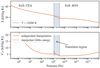 |
Fig. 1 Comparison between two possible methods of combining two equations of state. The solid lines correspond to interpolating all first and second order derivatives of the Gibbs potential independently, while for the dashed lines only the Gibbs free energy potential is interpolated and the derivatives of which calculated. |
2.2 Transition between equation of states
When using multiple EoS for the same material, special care needs to be taken when and how to transition between EoS. Considering two EoS in P–T space, two major cases need to be distinguished. In the first case the two EoS describe two different phases of H2O, hence a phase transition is expected to occur between the two EoS. The phase transition is, if present, the preferred location to transition between two EoS. By definition we expect discontinuities in the first and/or second order derivatives of the Gibbs free energy, hence no interpolation is needed to transition between two EoS. The location of the phase transition is either taken from experimental measurements or it is located where the two Gibbs energy potentials intersect Poirier (2000). The latter approach is preferential in terms of consistency, though it might sometimes not recover the experimentally determined location of a phase transition.
In the second case, no phase transition is expected to occur between the two EoS. One could naively think that interpolating either the Gibbs or Helmholtz free energy potential of the two EoS and calculating all thermodynamic quantities from the interpolatedpotential would then be sufficient. But such interpolation can introduce new discontinuities in the first and second order derivatives of the respective energy potential (see Fig. 1). Those discontinuities will even occur when using special interpolation methods as proposed for example by Swesty (1996) or Baturin et al. (2019). These methods are thought to consistently evaluate tabulated EoS data, but are not thought for functionally different EoS. But besides interpolating the free energy potentials, one can also interpolate all first and second order derivatives independently. Doing so, the aforementioned discontinuities are avoided, with the drawback that the thermodynamic consistency will not be guaranteed, since the thermodynamic variables will show deviations from Eqs. (3)–(18).
To illustrate this, in Fig. 1 we show a transition between two EoS without an interjacent phase transition. We see that if only the Gibbs free energy potential is interpolated (dashed lines), then discontinuities are introduced in the entropy and specific heat capacity, while interpolating all first and second order derivatives (solid lines) results in a smooth behaviour. Hence a choice between a smooth but slightly thermodynamically inconsistent transition or a discontinuous but thermodynamically consistent transition has to be made. Assuming that both EoS are valid in their own region, we opt for the smooth transition, avoiding arbitrarily introduced discontinuities as shown in Fig. 1.
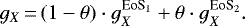
The two aforementioned cases lead to three methods that are used in this work to transition between EoS. The first method(in the following called Method 1) corresponds to the first case where a phase transition is expected between two EoS. There we locate the phase transition at the intersection of the Gibbs free energy potentials and change EoS at this location. If there is no interjacent phase transition (Method 2), then we define a transition region between the two EoS and interpolate in the first and second order derivatives of the Gibbs energy gX (P, T) using
 (19)
(19)
The interpolation factor θ is calculated using either
 (20)
(20)

depending on the orientation of the transition region. The location and extent of the transition region is heuristically determined with the goal of reducing the introduced thermodynamic inconsistencies. If the two neighbouring EoS are constructed such that they predictthe same thermodynamic variables in an overlapping region (Method 3), then no special steps need to be taken when transitioning between the EoS. The two EoS can then be simply connected along a line within the overlap region.
2.3 Pressure-temperature regions
We just saw that combining EoS can lead to potential inconsistencies. We therefore attempt to use as few EoS as possible. In a first step, the P–T space is split into seven regions for which a single EoS is chosen. If possible, the boundaries of the regions are located along phase transition curves. An overview of the regions is given in Table 1, where we also list which method was used to transition to the neighbouring EoS. Figure 2 further shows how the P–T space is split for the various EoS. The grey shaded areas in Fig. 2 show where there is no physical phase transition between regions and interpolation (i.e. Method 2) is needed to assure a smooth transition of the thermodynamic variables.
2.3.1 Region 1 (ice-Ih)
The first region spans over the stability region of ice-Ih, bounded by the melting and sublimation curves, as well as the ice-Ih/ice-II phase transition curve. For ice-Ih, the EoS from Feistel & Wagner (2006) is the canonical reference, adopted in the IAPWS-R10-06 release. It formulates a Gibbs energy potential and by design has a consistent transition when for the liquid and gas phase the EoS from the IAPWS-R6-95 release is used. The location of the melting and sublimation curves is then equal to the one described in Wagner et al. (2011).
Regions and the EoS used per region, as well as the method used to transition between two neighbouring regions.
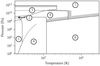 |
Fig. 2 Phase diagram of H2O split into the seven regions listed in Table 1. Most region boundaries (solid lines) follow phase transition curves. The dashed lines are phase transitions that are not region boundaries, meaning the same EoS is used along the phase transition. The shaded areas show where neighbouring regions have to be interpolated. Region 7, where the EoS of Mazevet et al. (2019) is used, expands to temperatures up to 105 K. |
2.3.2 Region 2 (ice-II, -III, -V and -VI)
For region 2 we use the EoS described in the recent work of Journaux et al. (2020). The EoS treats the ice-II, -III, -V, and -VI phases and can consistently calculate the stability region of the various phases. To evaluate the EoS we use the seafreeze-package3 of the same authors. Journaux et al. (2020) use local basis functions to fit a Gibbs energy potential to experimental data. The location of the phase transitions and region boundaries is calculated using the seafreeze-package, which also uses a Gibbs minimisation scheme to locate the phase transitions. For the location of the ice-VI/ice-VII phase transition, we use Method 1, which involves calculating where the Gibbs potential of regions 2 and 3 would intersect. We find that the fit
 (22)
(22)
parameterised the location of the phase transition between ice-VI and ice-VII up to the triple point at 2.216 GPa. The coefficients of Eq. (22) can be found in Table 2. Referring to the guidance of the seafreeze package, the use of the EoS of Bollengier et al. (2019) for the liquid phase along with the ice phases of the seafreeze package would be recommended in order to accurately recover the experimental location of the melting curves. But since the temperature range of Bollengier et al. (2019) is restricted to 500 K, we choose to use Brown (2018) in the neighbouring region 5. We tested if using Bollengier et al. (2019) would make a significant difference for the location of the melting curve. But changing to Bollengier et al. (2019) for T < 500 K only shifted the location given by Eq. (23) by a few Kelvin. Also the evaluated thermodynamic variables were equal, for example the maximal difference in density was 0.2%.
Coefficients for the fit of the melting pressure of ice-VII and ice-X as well as the phase transition curve between ice-VI and ice-VII.
2.3.3 Region 3 (ice-VII, ice-X)
The third region is the stability region of the high pressure ice phases of ice-VII and ice-X, where we use the EoS by French & Redmer (2015). They provide a Helmholtz free energy potential that can be evaluated in the entire stability region of ice-VII and ice-X, up to 2250 K. The melting curve that separates region 3 towards regions 5 and 7 was determined by minimising the Gibbs free energy; this is Method 1. We found that the melting pressure can then be calculated using the fit
![\begin{equation*} \log_{10} P_{\text{melt}}\,{=}\,\exp\left[x_1\cdot(T/c)^{x_2}+x_3\cdot(T/c)^{-1}+x_4\cdot(T/c)^{-3}\right] - 1,\end{equation*}](/articles/aa/full_html/2020/11/aa38367-20/aa38367-20-eq14.png) (23)
(23)
where Pmelt is in Pa and the coefficients of xi are given in Table 2. The melting curve of ice-X starts at 1634.6 K and goes up to 2250 K, from where it follows an isotherm. This cut-off at 2250 K is due to the limited range of the EoS, though it is similar to the experimental results of Schwager et al. (2004). Between 700 GPa and 1.5 TPa, ice-X is thought to undergo further structural changes until it transitions to the super-ionic phase (Militzer & Wilson 2010). Super-ionic water configurations are included in the ab initio calculations of M19, though at higher temperatures than 2250 K. We tried also adding the EoS of super-ionic water as in French et al. (2016) to our description, but no goodtransition back to the M19-EoS was found. Therefore, for pressures above 700 GPa we decided to use the M19-EoS.
2.3.4 Region 4 (gas, liquid, and supercritical fluid)
In region 4 we use the EoS from the IAPWS-R6-95 release (Wagner & Pruß 2002); this region spans over the entire liquid and the cold gas phase (<1200 K). The region boundaries follow the melting and sublimation curves from Wagner et al. (2011) up to 1 GPa. The IAPWS-R6-95 does not cover H2O vapour above 1273 K; we found that transitioning at 1200 K to the neighbouring region 6 results in a smooth transition (i.e. Method 3). The IAPWS-R6-95 is considered the canonical reference EoS for H2O in this P–T region. It is formulated as a Helmholtz free energy potential and reproduces experimental results well.
2.3.5 Region 5 (liquid and supercritical fluid)
Since pressures above 1 GPa are outside of the validity region of the IAPWS-R6-95, we use the EoS by Brown (2018) for region 5. Through the usage of local basis functions to fit a Gibbs energy potential, Brown (2018) provide an EoS that is appropriate for liquid and supercritical H2O from 1 to 100 GPa and up to 104 K. Brown (2018) used the IAPWS-R6-95 EoS as a basis for their work. In order to transition between regions 4 and 5, we simply switch the EoS at the boundary. The transition to regions 6 and 7 is discussed in their corresponding paragraph.
2.3.6 Region 6 (ideal gas)
At low densities, H2O vapour can be described as an ideal gas, though thermal effects, like dissociation and thermal ionisation require a more complex treatment than pure ideal gas. In region 6 we use the CEA (Chemical Equilibrium with Applications) package (Gordon & McBride 1994; McBride & Gordon 1996), which can calculate the EoS of water at these conditions up to 2 × 10⁴ K, including single ionisation and thermal dissociation. Besides the thermodynamic variables, in this regions we also calculate the mean molecular weight μ, the dissociation fraction xd, and the ionisation fraction xion, defined as
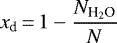 (24)
(24)

where N is the total particle number, NH2O the number of water molecules, and Ne the number of electrons. The following species are considered when the CEA package is evaluated: H2O, HO, H2, H, O2, and O, as well as the corresponding ions. In order to transition to regions 5 and 7, we use Method 2 along the transition region shown in Fig. 2.
2.3.7 Region 7 (superionic phase and supercritical fluid)
Region 7 corresponds to the M19-EoS. Mazevet et al. (2019) used Thomas-Fermi molecular dynamics (TFMD) simulations to construct a Helmholtz free energy potential up to densities of 100 g cm−3, which corresponds to pressures of ~400 TPa. Although the TFMD calculations were performed up to temperatures of 5 × 10⁴ K, we consider extrapolated values until 105 K. This range in P and T should be sufficient to model most of the conditions in the interior of giant planets.
Since there are no physical phase transitions between regions 4–7, we follow Method 2 in order to transition between the EoS. We tried to find transition regions in P–T space where the difference between neighbouring EoS is minimal. The transition region between regions 5 and 7 is bound towards region 5 by
 (26)
(26)
for temperatures between 1800 and 4500 K, followed by an isothermal part until the boundary of region 6, while towards region 7 it is bound by 1.5 ⋅ P5to7 until 5500 K. The border of the transition region between regions 6 and 7, for T >1000 K, is similarly given by
 (27)
(27)
and 3 ⋅ P6to7, while the borders of the transition region between regions 3 and 7 are at constant pressures of 300 and 700 GPa up to 2250 K. The transition regions are indicated as grey areas in Fig. 2. We only evaluate the M19-EoS down to 300 K, hence at high pressures and T < 300 K, the M19-EoS will be evaluated at constant temperature, though it is unlikely that water occurs in such conditions.
2.4 Energy and entropy shifts
The Gibbs and Helmholtz free energy potentials, as well as the internal energy and the entropy, are relative quantities. Hence they are defined in respect to a reference state. The IAPWS release for water provides two reference states. The first arbitrarily sets the internal energy and entropy at the triple point (Pt = 611.657 Pa, Tt = 273.16 K) to zero, while the second recovers the true physical zero point (P0 = 101325 Pa, T0 = 0 K) entropy of ice-1h as calculated by Nagle (1966). M19 on the other hand, uses the second reference point from IAPWS, but sets the internal energy to be always positive. In this work we will use the following reference state. At the zero point at P0 = 101325 Pa, T0 = 0 K, following Nagle (1966), the entropy is set to
 (28)
(28)
while the internal energy at the zero point is set to zero. This means that for all EoS used, the entropy and energy values need to be shifted accordingly to ensure consistent transitions of the entropy and energy potentials.
Since the reference state used by French & Redmer (2015) is not known, we shifted the energy potential in region 3 such that we recover the location of the ice-VI/VII/liquid triple point by Wagner et al. (2011). Table 3 provides an overview of the employed energy and entropy shifts.
Overview over the energy and entropy shifts used to construct the AQUA EoS.
3 Results
In the following section we discuss the properties of the AQUA EoS constructed with the method outlined in the last section. We validate said method and compare the thermodynamic variables calculated with the AQUA EoS to other EoS.
3.1 Tabulated equation of state
For better usability we provide tabulated values of the AQUA EoS on P–T, ρ–T, and ρ–U grids. Sincethe regions and their boundaries are given in P–T, the ρ–T and ρ–u grids are derived from the P–T grid. The fundamental P–T grid is calculated in the following way. For every point on the grid:
- 1.
we evaluate which region corresponds to the P, T values;
- 2.
we calculate either the Gibbs or Helmholtz free energy given the regions EoS;
- 3.
we evaluate either Eqs. (5)–(10) or Eqs. (11)–(18) to calculate ρ, s, u, w, ∇Ad;
- 4.
if the P,T values are in region 6, we calculate the dissociation and ionisation fractions Eqs. (24), (25) and the corresponding mean molecular weight;
- 5.
if the P,T values are in a transition region, we repeat steps (2) to (4) for the neighbouring region and transition between the two sets of thermodynamic variables as outlined in Sect. 2.2
The tabulated AQUA EoS is shown in Tables B.6–B.8. For the P–T table, we logarithmically sampled 70 points per decade from 0.1 Pa to 400 TPa and 100 points per decade from 102 to 105 K. The ρ–T table shares the same spacing along the temperature axis as the P–T table, while ρ was sampled logarithmically with 100 points per decade from 10−10 to 105 kg m−3. Similarly the ρ–U table shares the same ρ spacing as the ρ-T table, while the internal energy is logarithmically sampled with 100 points per decade from 105 to 4 × 10⁹ J kg−1. Due to its size, the tables are published in their entirety only at the CDS4.
3.2 Validation
In order to validate the method of combining the selected EoS, we check for the thermodynamic consistency of the created tabulated EoS using the relation
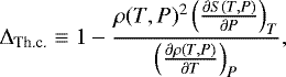 (29)
(29)
which is a measure of how well the caloric and mechanical parts of the EoS fulfil the fundamental thermodynamic relations used to derive Eqs. (5)–(18). A similar approach was chosen for example in Timmes & Arnett (1999) and Becker et al. (2014). Though since we use P and T as natural variables for our EoS, the equation for the thermodynamic consistency measure differs from said authors who use ρ and T. We derived Eq. (29) from the first law of thermodynamics in Appendix A. In Fig. 3 we show Eq. (29) evaluated over the P–T domain. As one can expect from EoS based on Gibbs or Helmholtz free energy potentials, within the different regions our method preserves thermodynamic consistency. Some inconsistencies can be seen at phase transitions between the ice phases as well as in the low pressure region of ice-1h, but they are rather small. The main inconsistencies are located between regions 5, 6, and 7. We would like to remind readers again that we attempt to create a formulation useful over large pressure and temperature scales. If an EoS is needed that is only used in a localised P–T domain, then other EoS will be more suitable. As already noted, we evaluate the M19-EoS above 400 GPa and below 300 K at constant temperature, therefore in this region thermodynamic consistency is also not given, but again this region is unlikely to be encountered in planets. Overall the method seems to deliver consistent results for the intended purpose of planetary structure modelling over a wide range of pressure and temperature.
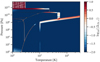 |
Fig. 3 Thermodynamic consistency measure δTh.c. defined in Eq. (29), as a function of pressure and temperature. Along phase transitions, the region boundaries, and around the critical point deviations from the ideal thermodynamic behaviour can be seen. The rectangular patch in the top left originates from evaluating the M19-EoS at constant temperature. |
3.3 Density ρ(P, T)
From all studied thermodynamic variables, the ρ–P–T relation of H2O will have the biggest impact on the mass radius relation of planets. In Fig. 4 we plotted ρ(P, T) using the AQUA EoS from 1 Pa to 400 TPa and 150 to 3 × 10⁴ K. At higher temperatures, only the M19-EoS contributes to the AQUA EoS, so we forwent expanding the plot to this P–T region. Overlaid are with dot-dashed lines the adiabatic P,T profiles of a 5 M⊕ sphere of pure water for different surface temperatures of 200, 300, and 1000 K.
In Fig. 5 we compare the AQUA EoS against two common EoS for water used in planetary science, the Analytical Equation of State (ANEOS) by Thompson (1990) using parameters for water as in Mordasini (2020) and an improved version of the quotidian equation of state (QEOS, priv. comm. and Vazan et al. 2013; Vazan & Helled 2020). In the same figure we also show the comparison against the pure M19-EoS. Each panel in Fig. 5 shows the density difference in percent between the AQUA EoS and the corresponding EoS of each panel calculated using
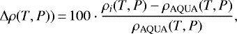 (30)
(30)
where the index i represents the EoS against which the difference in density is calculated. We note that both ANEOS and QEOS predict consistently lower densities at high pressures (>10 GPa). In contrast, the density of ice-Ih is predicted to be higher than in the AQUA EoS or as in Feistel & Wagner (2006). In the gas phase below 1 GPa, ANEOS predicts continuously lower densities, similar differences are seen for QEOS except above 2000 K where QEOS predicts slightly larger densities. QEOS has a significant shift in the location of the vapour curve and the location of the critical point.
For comparison we also evaluated the M19-EoS over the same P–T range. As expected no difference is seen at high pressures, since the same EoS is evaluated. At low pressures the density difference in the ice phases is visible, as are the large differences in the gaseous low density regions below 1 GPa.
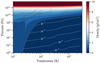 |
Fig. 4 Density of H2O as afunction of pressure and temperature calculated with the collection of H2O EoS of this work. The various EoS used to generate this plot are listed in Table 1. The solid black lines mark the phase transition between the solid, liquid, and gaseous phase. The white dashed lines are the density contours for the region where the density is below unity. The dot dashed black lines are adiabats calculated for a 5 M⊕ sphere of pure H2O for different surface temperatures of 200, 300, and 1000 K. |
3.4 Adiabatic temperature gradient ∇Ad (P, T)
The dimensionless adiabatic temperature gradient ∇Ad(P, T) is a key quantity to study the convective heat transport of a planet. In Fig. 6 we show the ∇Ad(P, T) of the AQUA EoS, ANEOS, and QEOS.
Compared to the AQUA EoS, the adiabatic gradient of ANEOS in the ice-Ih, liquid, and cold gas phase is similar, while QEOS shows a larger gradient and a shifted vapour curve. In the gas phase, ANEOS shows a region of low adiabatic gradient between 1000 and 1100 K, while for AQUA EoS a similar feature caused by thermal dissociation is visible but at higher temperatures. At the same time, ANEOS does not include thermal ionisation effects, which cause the second depression of ∇Ad in AQUA between 6000 and 10 000 K. In QEOS none of these features are present. Since in both AQUA EoS and ANEOS, the liquid and low pressure ice regions ∇Ad(P, T) is close to zero, this will lead to an almost isothermal temperature profile. Therefore any adiabatic temperature profile starting in one of these regions will stay in its solid or liquid state until it eventually reaches the high pressure ices phases. Starting in the vapour phase will cause the temperature profile to be steep enough to remain in the vapour phase and then transition to the supercritical region. All EoS show numerical artefacts at low temperatures and high pressure, though it is unlikely that planetary models will need this part of P–T space.
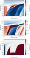 |
Fig. 5 Difference in density between the AQUA EoS and ANEOS (top panel), QEOS (middle panel), and the M19-EoS (bottom panel). A positive difference means that the AQUA EoS predicts a lower density in the specific location compared to the corresponding EoS of each panel. |
3.5 Entropy s(P, T), internal energy u(P, T)
As with the other variables we compare the results of the entropy and internal energy calculations with predictions by ANEOS and QEOS. In Figs. 7 and 8 we show in the top panel the entropy and internal energy predictions by AQUA as a function of P and T, while in the middle panel we show the relative differences compared to ANEOS and in the bottom panel compared to QEOS. The differences are calculated in the same way as for the density in Eq. (30). Compared to ANEOS the largest differences occur in the region where H2O dissociates. Both entropy and energy differ in this region by a factor of two. For the other part in P–T space the results for the internal energy do not differ by more than ± 25%, except a small region in the high pressure ice phases. In contrast, the entropy of ANEOS is significantly higher in the region of the high pressure ices between 1010 and 1012 Pa. This is likely due to the fact that the location of the melting curve in ANEOS is at a much lower temperature than that of AQUA.
While the energies and entropies of ANEOS were always within the same order of magnitude, the predictions of QEOS seem to be globally shifted. Compared to AQUA the energies are on average ~ 37.5 kJ g−1 larger while the entropies are ~ 2 J (gK)−1 smaller. This shift likely originates from a different choice of reference state, though since this information is not provided in Vazan et al. (2013), we can not be certain. Hence for most of P–T space, the entropies of QEOS are 50–75% smaller than those of AQUA. Only in the low temperature vapour region is the entropy a few percent larger. Regarding the internal energies, a shift of 37.5 kJ g−1 means that for pressures below ~1010 Pa and temperatures below ~2000 K, the predictions of AQUA and QEOS differ by multiple orders of magnitude. Assuming that this shift is due to a different reference state, in Fig. 8 we show the difference in energy if the internal energy potential of QEOS were 37.5 kJ g−1 smaller. We see that compared to ANEOS the spread in differences is larger. Some differences can be attributed to the shifted vapour curve, while we do not see a strong effect of the melting curve as we do with ANEOS. However, the energy of ice VI is notably smaller than the energy of ice VII and the other low pressure ices. Due to the applied shift in energy, the differences especially at low pressures can not be accurately determined.
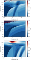 |
Fig. 6 Adiabatic temperature gradient of ANEOS (top panel), QEOS (bottom panel), and the AQUA EoS (bottom panel) as a function of pressure and temperature. The black lines are the phase boundaries as in Fig. 4. |
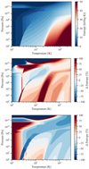 |
Fig. 7 Top panel: specific entropy of AQUA as a function of pressure and temperature. Middle panel: relative difference between the specific entropy of ANEOS vs. AQUA. Bottom panel: same comparison but between QEOS and AQUA. |
3.6 Bulk speed of sound w(P, T)
At last we show the results for the bulk speed of sound. Since QEOS of Vazan et al. (2013) does not provide the bulk speed of sound, we will compare in Fig. 9 only against ANEOS. Though in Fig. 10 we also show a comparison against experimental results of Lin & Trusler (2012) at low temperatures. Compared to ANEOS the bulk speed of sound is for most parts within ±40%. Notable differences occur throughout the dissociation region, around the critical point and within the region of ice-Ih. At high pressures (>1010 Pa) both ANEOS and AQUA results are within 10%.
In Fig. 10 one can see that due to the use of the IAPWS-95 EoS the bulk speed of sound of AQUA (solid lines) fits the experimental data of Lin & Trusler (2012) very well, while ANEOS (dashed lines) over-predicts the speed of sound at pressures below 108 Pa. Also ANEOS does not show a drop in the speed of sound at the vapour curve. For comparison we also show what the pure M19-EoS would predict (dotted lines). Like ANEOS it shows no drop at the vapour curve while predicting a generally lower speed of sound than AQUA.
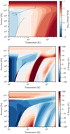 |
Fig. 8 Top panel: specific internal energy of AQUA as a function of pressure and temperature. Middle panel: relative difference between the internal energy of ANEOS vs. AQUA. Bottom panel: same comparison but between QEOS and AQUA. The internal energy potential of QEOS seems to be globally shifted compared to ANEOS and AQUA, probably due to a different choice of reference state. For the comparison we therefore subtracted 37.5 kJ g−1 from u(T, P)QEOS. |
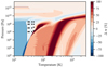 |
Fig. 9 Relative difference between the bulk speed of sound of ANEOS and AQUA as a function of pressure and temperature. The black dots indicate the location of the experimental data of Lin & Trusler (2012) shown in Fig. 10. |
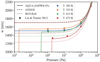 |
Fig. 10 Comparison of the bulk speed of sound between AQUA EoS (solid), ANEOS (dashed), the pure M19-EoS (dotted), and experimental results of Lin & Trusler (2012). We would like to point out that the compared range corresponds to regions 4 and 5. Hence AQUA EoS mainly evaluates the IAPWS-95 EoS and above 108 Pa the EoS of Brown (2018) is used. |
4 Effect on the mass radius relation of planets
4.1 Comparison of different equations of state
We see the main application of the AQUA EoS in the calculation of the internal structures of planets, exoplanets, and their moons. To test the effect of different EoS upon these calculations, we determine the mass radius relation for pure water spheres. As already stated by Mazevet et al. (2019), this is a purely academic exercise, but it is still useful since the results solely depend on the EoS used. In Appendix B we explain how we calculate the internal structure of a pure water sphere of given mass and determine its radius. We compare the AQUA EoS against ANEOS, QEOS, the H2O EoS used in Sotin et al. (2007), and the mass radius results of Zeng et al. (2019). Zeng et al. (2019) use a similar selection of EoS to the one proposed in this work, that is, Wagner & Pruß (2002), Frank et al. (2004), French et al. (2009) and French & Redmer (2015), but do not provide a publicly available EoS. Though we will use their results as a benchmark for our mass radius calculations. A more simple approach was chosen by Sotin et al. (2007), who on the other hand use two third order Birch-Murnaghan EoS: one isothermal for the liquid layer and one including temperature corrections for the high pressure ices. In Fig. 11 we show the result of the structure calculations for isothermal water spheres with masses between 0.25 and 20 M⊕. As in Zeng et al. (2019) we fixed the surface pressure to 1 mbar, while each panel shows the results for a different surface temperaturebetween 300 K and 1000 K.
We see that the choice of EoS has a strong effect on the radius for a given water mass. For ANEOS and QEOS one can predict that for large water mass fractions the radii for a given mass will be bigger, due to the lower density at high pressures. This featureis visible in all panels. The results of ANEOS are closer to AQUA than those of QEOS. For both the change in surface temperature does not strongly affect the relative differences compared to AQUA. On the contrary, the EoS used in Sotin et al. (2007) shows a bigger difference towards higher temperatures. This is due to the isothermal liquid layer and the absence of a vapour description in Sotin et al. (2007). But at 300 K the results only differ by − 0.8% to −3.69% for Sotin et al. (2007).
We report that the mass radius relation of Zeng et al. (2019) does predict very similar radii, within ± 2.5%. Except for afew low mass cases, larger radii are predicted. This is likely due to the fact that they do not compute a fully isothermal profile but follow the melting curve of the high pressure ices towards the super-ionic phase, as soon as the isotherm intersects the melting curve, which would lead to lower densities at high pressures.
The particular kink in the various mass radius relations at high surface temperatures and low water masses originates from the fact that there is not enough mass to create a steep enough pressure profile and for high enough temperatures the water sphere is then almost completely in the vapour phase, which results in inflated radii. This effect would be much more pronounced if an adiabatic temperature gradient was used, where even for lower surface temperatures the temperature profile would not cross the vapour curve.
For comparison we also plotted in dashed lines the mass radius relation for spheres with a 50 wt% H2O and 50 wt% Earth-like composition (i.e. 33.75 wt% MgSiO3 and 16.25 wt% Fe), as in Zeng et al. (2019). The results are also listed in Table B.5. For the EoS of the Fe core we used Hakim et al. (2018) and Sotin et al. (2007) for the MgSiO3 layer. In the300 K panel we also show the pure Earth-like composition case, in order to show that any difference in the 50 wt% H2O case stems from the H2O EoS. The difference in radius for the 50 wt% H2O case is about a factor two smaller than the difference in the pure H2O case: between −1% and 1.1% of relative difference.
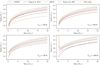 |
Fig. 11 Mass radius relations of isothermal spheres in hydrostatic equilibrium made of 100 wt.% H2O (solid lines) or 50 wt.% H2O and 50 wt.% Earth-like composition as in Zeng et al. (2019) (dashed lines), for different EoS and different surface temperatures Tsurf. The surfacepressure was chosen to be 1 mbar as in Zeng et al. (2019). For the cases with Earth-like composition, we used Hakim et al. (2018) as EoS for the Fe and Sotin et al. (2007) to calculate the density in the MgSiO3 layer. Top left panel: Earth-like composition case is also plotted (dotted lines) in order to quantify the contribution from the underlying rocky part to the cases of mixed composition. |
4.2 Adiabatic temperature gradient versus isothermal
For planets with significant amounts of volatile elements the proper treatment of thermal transport is of great importance for the mass radius calculation. We show here the effect of having a fully adiabatic temperature profile instead of an isothermal one, as was assumed in the last section.
Adiabatic processes follow an isentrope, as indicated by the dashed lines in Fig. 4. Hence if one starts below the vapour curve in the gas phase, the adiabat will never cross the vapour curve or one of the melting curves before the water becomes a supercritical fluid. But if we follow an isotherm from the same starting point, we reach the liquid phase at comparable low pressures where in the adiabatic case we would still be in the vapour phase. The adiabatic case resembles a post greenhouse state where all the water is fully mixed in the atmosphere.
In order to quantify this difference, we chose as in Sect. 5.1 of Mazevet et al. (2019), two masses of 0.5 M⊕ and 5 M⊕. For various surface temperatures we calculated the structure of a pure H2O sphere. We used the same model as in the last section, although we set the surface pressure to either the value of the vapour curve or 1 bar if above the critical temperature (as in Mazevet et al. 2019). We show in Fig. 12 the density as a function of radius for said two masses. We see that considering the two thermal structures, the density profile is considerably different at large surface temperatures (Tsurf > 1000 K), while at low surface temperatures (Tsurf < 300 K) it is almost equal. In the adiabatic case starting at 2000 K it is even below 2 × 10⁻⁴ g cm−3 throughout the structure. Here we see the effect of an increased adiabatic temperature gradient in the vapour phase compared to the liquid or solid phases. This effect is reduced if the water mass becomes larger and hence the sampled pressure scale increases simultaneously. In Table 4 we list the total radii of all cases shown in Fig. 12.
One has to remember that these results are based on calculations of pure water spheres; any addition of dense material will cause a steeper pressure profile and hence a more compact radius. We still conclude that the choice of thermal transport has a significant effect on the mass radius relation of a volatile layer made out of H2O.
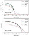 |
Fig. 12 Density profiles of a water sphere using either an isothermal temperature profile (solid) or an adiabatic temperature gradient (dashed). The surface temperatures are set to four different values (black = 300 K, green = 500 K, blue = 1000 K, red = 2000 K). Following a similar comparison from Mazevet et al. (2019), we set the surface pressure to the corresponding pressure on the vapour curve, unless the surface temperature is above the critical point, where the surface pressure is set to 1 bar. Bottom panel: the black dashed curve is overlapped by the solid black and green curves. |
Tabulated radii of a pure water sphere using either an adiabatic temperature gradient (RadiusAd) or an isothermal temperature profile (Radiusi.t.) and various surface temperatures.
5 Conclusions
We combined the H2O-EoS from Mazevet et al. (2019) with the EoS of Feistel & Wagner (2006), Journaux et al. (2020) and French & Redmer (2015) to include the description of ice phases at low, intermediate, and high pressures. For a proper treatment of the liquid phase and gas phase at low pressures, we added the EoS by Brown (2018), Wagner & Pruß (2002) and the CEA package (Gordon & McBride 1994; McBride & Gordon 1996) for the high temperature low pressure region. This resulted in the tabulated AQUA EoS5 providing data for the density ρ, adiabatic temperaturegradient ∇Ad, specific entropy s, specific internal energy u, and bulk speed of sound w, as well as the mean molecular weight μ, ionisation fraction xi and dissociation fraction xd for a limited region. The AQUA EoS offers a multi-phase description of all major phases of H2O useful to model the interiors of planets and exoplanets. We recommend the AQUA EoS for use in cases where thermodynamic data over a large range of pressures and temperatures are needed. However, by its construction, AQUA EoS is not fully thermodynamically consistent since it is not calculated from a single energy potential, but its consistency is sufficient for a large part of P–T space. Nevertheless we remind the reader again that we do not intend to offer a more accurate description than any EoS tailored to a limited region in P–T space but rather an EoS valid over a larger range of thermodynamical values.
We compared the values of the thermodynamics variables derived from the AQUA EoS against the values from ANEOS (Thompson 1990) and QEOS (Vazan et al. 2013; Vazan & Helled 2020). Compared to ANEOS and QEOS, AQUA shows a larger density at P >10 GPa, an effect which is already present in the original M19-EoS. At lower pressures the largest differences are seen in the region of ice-Ih and in the gas below 2000 K. For ∇Ad the results are more similar though not identical. For the entropy s and also the internal energy u, ANEOS predicts higher values by a factor of two throughout the dissociation region and along the melting curve of ice-Ih, while in most other regions s and u only differ by ~25% compared to AQUA. The only exception is within the ice-VII and ice-X region where the entropy is larger by a factor of two given a vastly colder melting curve of ice-VII/X in ANEOS. QEOS shows on average a ~ 2 J (g K)−1 lower entropy than AQUA. Also the internal energy potential u of QEOS seems shifted by 37.5 kJ g−1. Given that it is unclear if this shift stems from a different reference point, the comparison of s and u to AQUA is likely not very accurate. For the bulk speed of sound w we compared against ANEOS and the experimental values of Lin & Trusler (2012), since QEOS does not provide this thermodynamic quantity. ANEOS shows the largest differences at pressures below 109 Pa, while given the use of the IAPWS-95 release, AQUA agrees very well with the results of Lin & Trusler (2012).
We further studied the effect of different EoS on the mass radius relation of pure H2O spheres. Within ±2.5% we reproduce the values of Zeng et al. (2019) who use a similar selection of EoS. The other tested EoS (ANEOS, QEOS, and Sotin et al. 2007) show much bigger deviations from the radii we calculated. Deviations are between 3 and 8% for ANEOS and between 7 and 14% for QEOS, excluding the low water mass cases (≤ 0.5 M⊕) where the differences for high temperatures can be larger than 10%. The H2O EoS of Sotin et al. (2007) is mainly suited for low surface temperatures since it does not incorporate any vapour phase. For surface temperatures around 300 K it consistently predicts a smaller radius for a given mass by −0.8 to −3.6%, even thoughwe focused in this part on isothermal structures of pure water spheres, which is a mere theoretical test. The differences between EoS are still significant, especially in the view of improved radius estimates from upcoming space-based telescopes such as CHEOPS (Benz et al. 2017) or PLATO (Rauer & Heras 2018). Future work will be needed to unify the description of the thermodynamic properties of water over a wide range of pressures and temperatures.
In the last part we showed that the effect of surface temperature on the total radius is much bigger when we assume an adiabatic temperature profile instead of an isothermal one. This emphasises the importance of a proper treatment of the thermal part of the EoS used when modelling the structure of volatile rich planets.
Acknowledgements
We thank the anonymous referee for their valuable comments. We also thank Julia Venturini for the help implementing the CEA code and for various fruitful discussions. Further, we would like to thank Allona Vazan to provide to us her updated QEOS table for H2O. J.H. acknowledges the support from the Swiss National Science Foundation under grant 200020_172746 and 200020_19203. C.M. acknowledges the support from the Swiss National Science Foundation from grant BSSGI0_155816 “PlanetsInTime”. For this publication the following software packages have been used: Python 3.6, CEA (Chemical Equilibrium with Applications) (Gordon & McBride 1994; McBride & Gordon 1996), Python-iapws, Python-numpy, Python-matplotlib, Python-scipy, Python-seaborn, Python-seafreeze (Journaux et al. 2020).
Appendix A Derivation of the thermodynamic consistency measure
Unlike otherauthors who use ρ and T as natural variables for their EoS, we choose to use P and T instead. Therefore, the thermodynamic consistency measure used for example in Becker et al. (2014) needs to be reformulated for the use of P and T as natural variables. We start with the fundamental thermodynamic relation in terms of the internal energy U,
 (A.1)
(A.1)
Then we replace the differentials of the internal energy, entropy, and the volume with the relations

and sort the pressure and temperature derivatives to one side of the equation each,
 (A.5)
(A.5)
Using Bridgman’s thermodynamic equations (Bridgman 1914), we can replace some of the partial derivatives using the relations

Hence Eq. (A.5) can be written as
 (A.9)
(A.9)
Next, we can divide both sides by T ⋅dP, which results in one of the Maxwell relations,
 (A.10)
Similar to Becker et al. (2014), we define a measure of thermodynamic consistency, which compares the caloric left-hand side of Eq. (A.10) with the mechanical right-hand side:
 (A.11)
Appendix B Structure model
To determine the mass radius relation for pure H2O spheres (or 50 wt.% H2O when compared to Zeng et al. 2019), we solve the mechanical and thermal structure equations in the Lagrangian notation, as in Kippenhahn et al. (2012) for stellar structures. We assume a constant luminosity throughout the structure, meaning we neglect potential heat sources within the planet. The remaining structure equations for a static, 1D, spherically symmetric sphere in hydrostatic equilibrium are then given by

where ∇Ad is the adiabatic temperature gradient as defined in Eq. (2), r is the radius, m is the mass within radius r, P is the pressure, and T the temperature. For a given total mass, surface pressure, and surface temperature we use a bidirectional shooting method to solve the two point boundary value problem posed by Eqs. (B.1)–(B.3). The equations are integrated using a fifth order Cash-Karp Runge-Kutta method, similar to the one described in Press et al. (1996). From this calculation we get the mechanical and thermal structure as a function of m, from which we can extract the total radius at m = Mtot. If not stateddifferently, the surface pressure is set to 1 mbar as in Zeng et al. (2019), which is a first order approximation of the depth of thetransit radius.
At eachnumerical step in the Runge-Kutta method, the equation of state is evaluated to determine ρ(P, T) and ∇Ad(P, T). For an isothermal structure, ∇Ad(P, T) is simply set to zero. As described in the main text we test various water equations of state. In the case where we compare with the results of Zeng et al. (2019) we split the structure into three layers: an iron core using the EoS of Hakim et al. (2018) (16.25 wt.%), a silicate mantle as in Sotin et al. (2007) (33.75 wt.%), and a water layer (50 wt.%). Similar to this work, Zeng et al. (2019) use multiple EoS for the water layer: Wagner & Pruß (2002), Frank et al. (2004), French et al. (2009), and French & Redmer (2015).
Mass radius relation for isothermal pure H2O spheres and various EoS.
Mass radius relation for isothermal pure H2O spheres and various EoS.
Mass radius relation for isothermal pure H2O spheres and various EoS.
Mass radius relation for isothermal pure H2O spheres and various EoS.
Mass radius relation for isothermal spheres with 50 wt.% H2O, 33.75 wt.% MgSiO3 and 16.25 wt.% Fe.
AQUA equation of state for water, as a function of pressure and temperature.
AQUA equation of state for water, tabulated as a function of density and temperature.
AQUA equation of state for water, tabulated as a function of density and internal energy.
References
- Allen, J. F., Raven, J. A., Martin, W., & Russell, M. J. 2003, Phil. Trans. R. Soc.London Ser. B Biol. Sci., 358, 59 [CrossRef] [Google Scholar]
- Baturin, V. A., Däppen, W., Oreshina, A. V., Ayukov, S. V., & Gorshkov, A. B. 2019, A&A, 626, A108 [CrossRef] [EDP Sciences] [Google Scholar]
- Becker, A., Lorenzen, W., Fortney, J. J., et al. 2014, ApJS, 215, 21 [NASA ADS] [CrossRef] [Google Scholar]
- Benz, W., Ehrenreich, D., & Isaak, K. 2017, in Handbook of Exoplanets, eds. H. J. Deeg, & J. A. Belmonte (Cham: Springer International Publishing), 1 [Google Scholar]
- Bollengier, O., Brown, J. M., & Shaw, G. H. 2019, J. Chem. Phys., 151, 054501 [CrossRef] [Google Scholar]
- Bridgman, P. W. 1914, Phys. Rev., 3, 273 [CrossRef] [Google Scholar]
- Brown, J. M. 2018, Fluid Phase Equilib., 463, 18 [CrossRef] [Google Scholar]
- Callen, H. B. 1985, Thermodynamics and an Introduction to Thermostatistics, 2nd edn. (Weinheim: Wiley-VCH), 512 [Google Scholar]
- Feistel, R., & Wagner, W. 2006, J. Phys. Chem. Ref. Data, 35, 1021 [NASA ADS] [CrossRef] [Google Scholar]
- Frank, M. R., Fei, Y., & Hu, J. 2004, Geochim. Cosmochim. Acta, 68, 2781 [CrossRef] [Google Scholar]
- French, M., & Redmer, R. 2015, Phys. Rev. B, 91, 014308 [NASA ADS] [CrossRef] [Google Scholar]
- French, M., Mattsson, T. R., Nettelmann, N., & Redmer, R. 2009, Phys. Rev. B, 79, 054107 [NASA ADS] [CrossRef] [Google Scholar]
- French, M., Desjarlais, M. P., & Redmer, R. 2016, Phys. Rev. E, 93, 022140 [NASA ADS] [CrossRef] [Google Scholar]
- Gordon, S., & McBride, B. J. 1994, Computer Program for Calculation of Complex Chemical Equilibrium Compositions and Applications. Part 1: Analysis, Tech. rep., NASA Lewis Research Center [Google Scholar]
- Grasset, O., Castillo-Rogez, J., Guillot, T., Fletcher, L. N., & Tosi, F. 2017, Space Sci. Rev., 212, 835 [CrossRef] [Google Scholar]
- Hakim, K., Rivoldini, A., Van Hoolst, T., et al. 2018, Icarus, 313, 61 [NASA ADS] [CrossRef] [Google Scholar]
- Journaux, B., Brown, J. M., Pakhomova, A., et al. 2020, J. Geophys. Res. Planets, 125, e2019JE006176 [Google Scholar]
- Kippenhahn, R., Weigert, A., & Weiss, A. 2012, Stellar Structure and Evolution, 2nd edn., Astron. Astrophys. Lib. (Berlin Heidelberg: Springer-Verlag) [CrossRef] [Google Scholar]
- Lin, C.-W., & Trusler, J. P. M. 2012, J. Chem. Phys., 136, 094511 [CrossRef] [Google Scholar]
- Mazevet, S., Licari, A., Chabrier, G., & Potekhin, A. Y. 2019, A&A, 621, A128 [NASA ADS] [CrossRef] [EDP Sciences] [Google Scholar]
- McBride, B. J., & Gordon, S. 1996, Computer Program for Calculation of Complex Chemical Equilibrium Compositions and Applications II. Users Manual and Program Description, Tech. rep., NASA Lewis Research Center [Google Scholar]
- Militzer, B., & Wilson, H. F. 2010, Phys. Rev. Lett., 105, 195701 [CrossRef] [Google Scholar]
- Mordasini, C. 2020, A&A, 638, A52 [CrossRef] [EDP Sciences] [Google Scholar]
- Nagle, J. F. 1966, J. Math. Phys., 7, 1484 [CrossRef] [Google Scholar]
- Poirier, J.-P. 2000, Introduction to the Physics of the Earth’s Interior, 2nd edn. (Cambridge: Cambridge University Press) [CrossRef] [Google Scholar]
- Press, W. H., Teukolsky, S. A., Vetterling, W. T., & Flannery, B. P. 1996, Numerical Recipes in Fortran 90: Volume 2, Volume 2 of Fortran Numerical Recipes: The Art of Parallel Scientific Computing (Cambridge: Cambridge University Press) [Google Scholar]
- Rauer, H., & Heras, A. M. 2018, in Handbook of Exoplanets, eds. H. J. Deeg, & J. A. Belmonte (Cham: Springer International Publishing), 1309 [CrossRef] [Google Scholar]
- Schwager, B., Chudinovskikh, L., Gavriliuk, A., & Boehler, R. 2004, J. Phys. Cond. Matter, 16, S1177 [NASA ADS] [CrossRef] [Google Scholar]
- Senft, L. E., & Stewart, S. T. 2008, Meteorit. Planet. Sci., 43, 1993 [CrossRef] [Google Scholar]
- Sotin, C., Grasset, O., & Mocquet, A. 2007, Icarus, 191, 337 [NASA ADS] [CrossRef] [Google Scholar]
- Swesty, F. D. 1996, J. Comput. Phys., 127, 118 [NASA ADS] [CrossRef] [Google Scholar]
- Thompson, S. L. 1990, ANEOS analytic equations of state for shock physics codes input manual, Tech. rep., Sandia National Labs [CrossRef] [Google Scholar]
- Thorade, M., & Saadat, A. 2013, Environ. Earth Sci., 70, 3497 [CrossRef] [Google Scholar]
- Timmes, F. X., & Arnett, D. 1999, ApJS, 125, 277 [NASA ADS] [CrossRef] [Google Scholar]
- van Dishoeck, E. F., Bergin, E. A., Lis, D. C., & Lunine, J. I. 2014, in Protostars and Planets VI, eds. H. Beuther, R. S. Klessen, C. P. Dullemond, & T. Henning (Tucson, AZ: University of Arizons Press), 835 [Google Scholar]
- Vazan, A., & Helled, R. 2020, A&A, 633, A50 [CrossRef] [EDP Sciences] [Google Scholar]
- Vazan, A., Kovetz, A., Podolak, M., & Helled, R. 2013, MNRAS, 434, 3283 [NASA ADS] [CrossRef] [Google Scholar]
- Wagner, W., & Pruß, A. 2002, J. Phys. Chem. Ref. Data, 31, 387 [NASA ADS] [CrossRef] [Google Scholar]
- Wagner, W., Riethmann, T., Feistel, R., & Harvey, A. H. 2011, J. Phys. Chem. Ref. Data, 40, 043103 [NASA ADS] [CrossRef] [Google Scholar]
- Wiggins, P. 2008, PLOS One, 3, e1406 [CrossRef] [Google Scholar]
- Zeng, L., Jacobsen, S. B., Sasselov, D. D., et al. 2019, Proc. Natl. Acad. Sci., 116, 9723 [Google Scholar]
Although the results of Wagner & Pruß (2002) are used by Mazevet et al. (2019) to improve the provided fit towards lower temperatures.
The tables are also available to download under the link https://github.com/mnijh/AQUA
Available at https://github.com/mnijh/aqua
All Tables
Regions and the EoS used per region, as well as the method used to transition between two neighbouring regions.
Coefficients for the fit of the melting pressure of ice-VII and ice-X as well as the phase transition curve between ice-VI and ice-VII.
Tabulated radii of a pure water sphere using either an adiabatic temperature gradient (RadiusAd) or an isothermal temperature profile (Radiusi.t.) and various surface temperatures.
Mass radius relation for isothermal spheres with 50 wt.% H2O, 33.75 wt.% MgSiO3 and 16.25 wt.% Fe.
AQUA equation of state for water, tabulated as a function of density and temperature.
AQUA equation of state for water, tabulated as a function of density and internal energy.
All Figures
|
Fig. 1 Comparison between two possible methods of combining two equations of state. The solid lines correspond to interpolating all first and second order derivatives of the Gibbs potential independently, while for the dashed lines only the Gibbs free energy potential is interpolated and the derivatives of which calculated. |
| In the text | |
|
Fig. 2 Phase diagram of H2O split into the seven regions listed in Table 1. Most region boundaries (solid lines) follow phase transition curves. The dashed lines are phase transitions that are not region boundaries, meaning the same EoS is used along the phase transition. The shaded areas show where neighbouring regions have to be interpolated. Region 7, where the EoS of Mazevet et al. (2019) is used, expands to temperatures up to 105 K. |
| In the text | |
|
Fig. 3 Thermodynamic consistency measure δTh.c. defined in Eq. (29), as a function of pressure and temperature. Along phase transitions, the region boundaries, and around the critical point deviations from the ideal thermodynamic behaviour can be seen. The rectangular patch in the top left originates from evaluating the M19-EoS at constant temperature. |
| In the text | |
|
Fig. 4 Density of H2O as afunction of pressure and temperature calculated with the collection of H2O EoS of this work. The various EoS used to generate this plot are listed in Table 1. The solid black lines mark the phase transition between the solid, liquid, and gaseous phase. The white dashed lines are the density contours for the region where the density is below unity. The dot dashed black lines are adiabats calculated for a 5 M⊕ sphere of pure H2O for different surface temperatures of 200, 300, and 1000 K. |
| In the text | |
|
Fig. 5 Difference in density between the AQUA EoS and ANEOS (top panel), QEOS (middle panel), and the M19-EoS (bottom panel). A positive difference means that the AQUA EoS predicts a lower density in the specific location compared to the corresponding EoS of each panel. |
| In the text | |
|
Fig. 6 Adiabatic temperature gradient of ANEOS (top panel), QEOS (bottom panel), and the AQUA EoS (bottom panel) as a function of pressure and temperature. The black lines are the phase boundaries as in Fig. 4. |
| In the text | |
|
Fig. 7 Top panel: specific entropy of AQUA as a function of pressure and temperature. Middle panel: relative difference between the specific entropy of ANEOS vs. AQUA. Bottom panel: same comparison but between QEOS and AQUA. |
| In the text | |
|
Fig. 8 Top panel: specific internal energy of AQUA as a function of pressure and temperature. Middle panel: relative difference between the internal energy of ANEOS vs. AQUA. Bottom panel: same comparison but between QEOS and AQUA. The internal energy potential of QEOS seems to be globally shifted compared to ANEOS and AQUA, probably due to a different choice of reference state. For the comparison we therefore subtracted 37.5 kJ g−1 from u(T, P)QEOS. |
| In the text | |
|
Fig. 9 Relative difference between the bulk speed of sound of ANEOS and AQUA as a function of pressure and temperature. The black dots indicate the location of the experimental data of Lin & Trusler (2012) shown in Fig. 10. |
| In the text | |
|
Fig. 10 Comparison of the bulk speed of sound between AQUA EoS (solid), ANEOS (dashed), the pure M19-EoS (dotted), and experimental results of Lin & Trusler (2012). We would like to point out that the compared range corresponds to regions 4 and 5. Hence AQUA EoS mainly evaluates the IAPWS-95 EoS and above 108 Pa the EoS of Brown (2018) is used. |
| In the text | |
|
Fig. 11 Mass radius relations of isothermal spheres in hydrostatic equilibrium made of 100 wt.% H2O (solid lines) or 50 wt.% H2O and 50 wt.% Earth-like composition as in Zeng et al. (2019) (dashed lines), for different EoS and different surface temperatures Tsurf. The surfacepressure was chosen to be 1 mbar as in Zeng et al. (2019). For the cases with Earth-like composition, we used Hakim et al. (2018) as EoS for the Fe and Sotin et al. (2007) to calculate the density in the MgSiO3 layer. Top left panel: Earth-like composition case is also plotted (dotted lines) in order to quantify the contribution from the underlying rocky part to the cases of mixed composition. |
| In the text | |
|
Fig. 12 Density profiles of a water sphere using either an isothermal temperature profile (solid) or an adiabatic temperature gradient (dashed). The surface temperatures are set to four different values (black = 300 K, green = 500 K, blue = 1000 K, red = 2000 K). Following a similar comparison from Mazevet et al. (2019), we set the surface pressure to the corresponding pressure on the vapour curve, unless the surface temperature is above the critical point, where the surface pressure is set to 1 bar. Bottom panel: the black dashed curve is overlapped by the solid black and green curves. |
| In the text | |
Current usage metrics show cumulative count of Article Views (full-text article views including HTML views, PDF and ePub downloads, according to the available data) and Abstracts Views on Vision4Press platform.
Data correspond to usage on the plateform after 2015. The current usage metrics is available 48-96 hours after online publication and is updated daily on week days.
Initial download of the metrics may take a while.