| Issue |
A&A
Volume 681, January 2024
|
|
|---|---|---|
| Article Number | A96 | |
| Number of page(s) | 26 | |
| Section | Planets and planetary systems | |
| DOI | https://doi.org/10.1051/0004-6361/202346965 | |
| Published online | 23 January 2024 | |
BICEPS: An improved characterization model for low- and intermediate-mass exoplanets
1
Weltraumforschung und Planetologie, Physikalisches Institut,
Gesellschaftsstrasse 6,
3012
Bern, Switzerland
e-mail: This email address is being protected from spambots. You need JavaScript enabled to view it.
2
Abteilung Physik, Gymnasium Lerbermatt,
Kirchstrasse 64,
3098
Köniz, Switzerland
3
Institute for Particle Physics and Astrophysics,
Wolfgang-Pauli-Strasse 27,
8093
Zurich, Switzerland
4
Observatoire Astronomique de l’Université de Genève,
Chemin Pegasi 51, Sauverny,
1290
Versoix, Switzerland
Received:
22
May
2023
Accepted:
16
October
2023
Abstract
Context. The number of exoplanets with precise mass and radius measurements is constantly increasing thanks to novel ground- and space-based facilities such as HARPS, ESPRESSO, CHEOPS, and TESS. The accuracy and robustness of the planetary characterization largely depends on the quality of the data, but also requires a planetary structure model, capable of accurately modeling the interior and atmospheres of exoplanets over a large range of boundary conditions.
Aims. Our goal is to provide an improved characterization model for planets with masses between 0.5 and 30 Earth masses, equilibrium temperatures below <2000 K, and a wide range of planetary compositions and physical phases.
Methods. In this work, we present the Bayesian Interior Characterization of ExoPlanetS (BICEPS) model, which combines an adaptive Markov chain Monte Carlo sampling method with a state-of-the-art planetary structure model. BICEPS incorporates many recently developed equations of state suited for large ranges of pressures and temperatures, a description for solid and molten planetary cores and mantles, a gaseous envelope composed of hydrogen, helium, and water (with compositional gradients), and a non-gray atmospheric model.
Results. We find that the usage of updated equations of state has a significant impact on the interior structure prediction. The impact varies, depending on the planetary composition. For dense rocky planets, BICEPS predicts radii a few percent different to prior internal structure models. For volatile rich planets, we find differences of 10% or even larger. When applying BICEPS to a particular exoplanet, TOI-130 b, we inferred a 25% larger water mass fraction and a 15% smaller core than previous models.
Conclusions. The presented exoplanet characterization model is a robust method applicable over a large range of planetary masses, compositions, and thermal boundary conditions. We show the importance of implementing state-of-the-art equations of state for the encountered thermodynamic conditions of exoplanets. Hence, using BICEPS improves the predictive strength of the characterization process compared to previous methods.
Key words: planets and satellites: interiors / planets and satellites: composition / methods: numerical / methods: statistical / equation of state
© The Authors 2024
 Open Access article, published by EDP Sciences, under the terms of the Creative Commons Attribution License (https://creativecommons.org/licenses/by/4.0), which permits unrestricted use, distribution, and reproduction in any medium, provided the original work is properly cited.
This article is published in open access under the Subscribe to Open model. This email address is being protected from spambots. You need JavaScript enabled to view it. to support open access publication.
1 Introduction
The determination of an exoplanet’s composition and internal structure is one of the key challenges in planetary sciences. Knowing an exoplanet’s composition not only informs us about the properties of the studied exoplanet, but it also helps for formation and evolution to be constrained (Venturini et al. 2020a; Adibekyan et al. 2021). In this work we present an improved method to characterize core-dominated exoplanets with masses between 0.5 mE and 30 mE.
Characterizing an exoplanet is a challenging task, given the very limited information available. For most exoplanets we only know their orbital period and either their mass or radius, but not both. We also have mostly no observational evidence for their elemental composition, besides for some gas-rich, short period exoplanets where one can use spectroscopy to determine the atmospheric composition (e.g., Benneke & Seager 2012; Chubb et al. 2020; Khalafinejad et al. 2021). However, only when both the mass and radius of an exoplanet are known can one calculate the exoplanet’s mean density, which is a direct consequence of a planet’s composition1. In order to relate the exoplanet’s mass, radius, and composition, one needs a model of the planetary interior. In the literature one can find a vast number of internal structure models for various types of exoplanets and of different physical complexity (see, e.g., Valencia et al. 2006; Seager et al. 2007; Sotin et al. 2007; Vazan et al. 2013; Unterborn et al. 2016; van den Berg et al. 2019; Boujibar et al. 2020; Acuña et al. 2021; Huang et al. 2022).
Most approaches found in the literature use a Bayesian inference method for calculating this conditional probability, that is, Markov chain Monte Carlo (MCMC) sampling (Dorn et al. 2015, 2017, hereafter called D15 and D17; Acuña et al. 2021) or nested sampling (Otegi et al. 2020). Recently some authors also proposed various machine learning techniques instead (e.g., Baumeister et al. 2020; Zhao & Ni 2021 ; Haldemann et al. 2023).
The number of exoplanets for which both the mass and radius are known is rapidly increasing. Large observational efforts are undertaken using both ground-based facilities such as the High Accuracy Radial velocity Planet Searcher (HARPS; Mayor et al. 2003) or the Echelle SPectrograph for Rocky Exoplanets and Stable Spectroscopic Observations (ESPRESSO; Pepe et al. 2014), as well as space-based instruments such as the Transiting Exoplanet Survey Satellite (TESS; Ricker et al. 2014) and the CHaracterising ExOPlanet Satellite (CHEOPS; Benz et al. 2021). In addition to increasing the number of exoplanets that can be characterized, these missions also help to drastically reduce the observational uncertainties as to the mass and radius (see, e.g., Sozzetti et al. 2021). Reducing the observational uncertainty as to the mass and radius ultimately leads to better constraints on an exoplanet’s composition. However, even with very accurate data, the inherent degeneracy that multiple compositions can lead to the same mean density remains.
It was shown that using the ratios of the refractory elements Mg, Si, and Fe in the host star’s photosphere as a proxy for the composition of the exoplanet can help this degeneracy be reduced (D15; D17). As the refractory elements Mg, Si, and Fe condense out from the protoplanetary disk at similar temperatures, it is expected that the growing planets that accrete from this condensed material retain the relative elemental abundances of the refractory elements. This assumption is also supported by numerical simulations (e.g., Thiabaud et al. 2015) as well as Solar System observations (e.g., Sotin et al. 2007), although studies of observed exoplanets that attempted to test this assumption statistically are not yet conclusive (Plotnykov & Valencia 2020; Schulze et al. 2021; Adibekyan et al. 2021). This approach works best for planets that have a high mean density, that is to say they are dominated by a rocky mantle and an iron core. However, for exoplanets with mean densities between 2 and 4 g cm−3 that contain more volatile elements, the degeneracy between a different composition is harder to overcome (Otegi et al. 2020).
To fully leverage the exquisite observational data, it is therefore important to reduce the theoretical uncertainties introduced by the planetary structure model. In the past years, considerable progress has been made in the description of matter under the extreme thermodynamic conditions of exoplanets, resulting in improved equations of state for many of the key building blocks of exoplanets (e.g., Mazevet et al. 2019; Musella et al. 2019; Ichikawa & Tsuchiya 2020; Haldemann et al. 2020; Kuwayama et al. 2020; Stewart et al. 2020).
In this work we include these recently developed equations of state to build a robust and efficient tool for exoplanet characterization, hereafter called Bayesian Interior Characterization of ExoPlanetS (BICEPS). BICEPS follows the basic concepts of previous planet characterization methods (D15; D17; Otegi et al. 2020; Acuña et al. 2021), combining an interior structure model with a Bayesian framework. Compared to these works, we updated the used equations of state and include the following: descriptions for solid and molten core and mantle layers (similar to Dorn & Lichtenberg 2021; Noack & Lasbleis 2020); the non-gray analytical atmosphere model of Parmentier & Guillot (2014) and Parmentier et al. (2015) together with the compositional dependent opacities of Freedman et al. (2014); a description of a compositional gradient of water in the envelope, such that water is not present past its saturation point; as well as many smaller improvements such as a more efficient sampling of the target posterior probability distribution by the MCMC method.
To demonstrate the performance of BICEPS, we compared our model to the original version of D17. While the structure model of D17 has been employed for planet characterizations, its original version has been adapted over the years to include molten mantle and core phases, numerous improved equations of state (see Haldemann 2021), and also the possibility of water dissolution in magma oceans (Dorn & Lichtenberg 2021). For simplicity, we used its original version for comparison purposes.
This work is structured as follows: in Sect. 2 we describe the internal structure model and the Bayesian method which together make up the BICEPS model. In Sect. 3, we explain how we performed a structure model comparison between BICEPS and the original model from D17. This model comparison was performed for all major model constituents as well as for a full characterization of the exoplanet TOI-130 b. In Sect. 4, we discuss the findings and also present a set of iso-composition curves useful for interpreting mass versus radius diagrams of exoplanets. Finally, in Sect. 5, we summarize the key aspects of our work.
2 Method
In this section we describe the BICEPS model, which consists of two major parts: First, a planetary structure model, which calculates for a given mass and composition of the exoplanet its structure and total radius, hereafter also called the forward model. Second, a MCMC method to calculate the posterior probability distribution over all forward model parameters, given prior information on the model parameters and observed mass, radius, orbital period of the exoplanet and refractory composition of the host star. This general approach was also used in other work (see D15; D17; Acuña et al. 2021).
2.1 General assumptions
The structure of an exoplanet is the result of a variety of physical and chemical processes acting on various temporal and spatial scales. This means one needs various interlinking descriptions to accurately model the internal structure of an exoplanet, which can result in very computationally expensive descriptions. At the same time, one needs a statistical method, such as an MCMC sampler, to infer an exoplanet’s composition. Given the many free parameters, a typical MCMC run requires 105–106 forward models to be calculated. In order to be computationally efficient, one has to make some simplifying assumptions when setting up the used planetary structure model. For BICEPS we make the following general assumptions.
The interior structure model describes a 1-D spherical symmetric sphere in hydrostatic equilibrium, which is made up of distinct layers of different composition (see Fig. 1). The major elemental constituents which we consider are: H, He, O, Fe, Si, Mg and S. In the center of the planet there is an iron core of mass mCore which can contain some less dense iron alloys, that is, FeS. The core is surrounded by a silicate mantle of mass mMantle made up of Fe, Mg, Si and O which form different minerals. The outermost volatile layer of mass mVol is made up of H, He and H2O. Depending on the thermal boundary conditions, the material in each layer can be in different phases, for instance, the core and mantle can be molten or the water can be liquid or in one of its many ice phases. More details on the considered phases are given in the corresponding paragraphs of each layer.
2.2 Planetary structure equations
The differential equations which are used to describe the thermal and mechanical structure of an exoplanet are similar to the ones used for stellar structure models (see, e.g., Kippenhahn et al. 2012): the equation of mass conservation
 (1)
(1)
the equation of hydrostatic equilibrium
 (2)
(2)
the thermal transport equation
 (3)
(3)
and the energy conservation equation
 (4)
(4)
The variables r, m, P, T, ρ, L, G, ϵ, and ∇ used in Eqs. (1)–(4) are the radius, mass inside radius r, pressure, temperature, density, luminosity, gravitational constant, energy generation rate per unit mass, and the dimensionless temperature gradient
 (5)
(5)
Depending on the layer and its composition, we use a different temperature gradient.
Solving the structure equations is a so-called two-point boundary value problem. We solve this two-point boundary value problem, by integrating Eqs. (1)–(4) for a given mass and composition, using a fifth order Cash-Karp Runge–Kutta method (Press et al. 1996). The structure equations are integrated both from the outside inward, and from the inside outward until reaching the core mantle boundary. Then the total radius and central boundary conditions are iterative adapted until the two integrations intersect at the core mantle boundary.
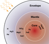 |
Fig. 1 Schematic representation of the interior structure model. The modeled exoplanet consists of three main layers: an iron core in the center, surrounded by a silicate mantle, below an envelope made out of volatile elements, irradiated by the host star. |
2.3 Core layer model
Iron is thought to be the dominant constituent in planetary cores, given its abundance compared to other refractory elements and its relative large density. It is also thought, that iron core formation is efficient enough that already moon sized objects likely host iron cores (Ricard et al. 2009). Thus, most exoplanets will likely host an iron core. In case of the Earth’s core, a lower density than pure Fe is inferred from seismic measurements (Dziewonski & Anderson 1981). Additional lighter elements than iron are needed to explain the density of Earth’s core. During core formation, other lighter elements can sink to the core, diluting the core with less dense iron-alloys. The nature and amount of the lighter core elements is unknown to this day, but likely candidates are S, Si, O, C and Ni (Ichikawa & Tsuchiya 2020).
In BICEPS, we consider a core made out of Fe and S (as in e.g., Sotin et al. 2007; Valencia et al. 2007). In the case of pure Fe we consider the phases ϵ-Fe, γ-Fe, δ-Fe and α-Fe, that is, the hexagonal close packed (hcp), face-centered cubic (fcc) and the two body-centered cubic (bcc) configurations as well as liquid Fe. For each phase we use a different EoS, that is, Hakim et al. (2018) and Fei et al. (2016) for ϵ-Fe, Dorogokupets et al. (2017) for γ-Fe, δ-Fe and α-Fe and for liquid-Fe we use the EoSs of Ichikawa & Tsuchiya (2020) and at pressures below 100 GPa (Kuwayama et al. 2020). For ϵ-Fe the EoS of Hakim et al. (2018) cannot be used at low pressures, hence as recommended in their publication we use Fei et al. (2016) below 234.4 GPa. The location of each phase boundary is based on empirical data, combining various sources. The melting curve of pure Fe is calculated following Anzellini et al. (2013), that is,
 (6)
(6)
with the pressure P having units of Pa, the reference point set at (P0 = 5.2 GPa, T0 = 1991 K) and the ϵ-γ-liquid-triple point set at (Pt = 98.5 GPa, Tt = 3712 K). The various phase transition curves between the low pressure iron phases are taken from Fig. 1 of Dorogokupets et al. (2017). The four phase transition curves are then given by:
 (7)
(7)
 (8)
(8)
 (9)
(9)
 (10)
(10)
We note that this approach is not fully thermodynamic consistent, but necessary, since there is no set of publicly available iron EoS which covers the necessary phase space and is formulated as a thermodynamic potential necessary to calculate the phase transitions in a more consistent manner. In Fig. 2, we show an overview over the resulting phase diagram of pure Fe.
As in Valencia et al. (2007), we assume that the sulfur alloy in the core will be FeS and that FeS will mix uniformly throughout the core. We neglect the various solid FeS phases and their stability regions (Bazhanova et al. 2017), but only consider one solid and one liquid FeS phase. We also assume, that the presence of sulfur only affects the location of the melting curve but not the solid to solid phase transitions of any pure iron phases. To incorporate the effect of S onto the melting curve, we introduce a correction factor which lowers the melting temperature proportional to the sulfur fraction (Stixrude 2014)
 (11)
(11)
where χFe is the molar fraction2 of Fe in the core, that is,
 (12)
(12)
The reasons why we forwent to implement a more complex phase diagram of the Fe–S system, are: that it is still unknown which lighter elements are present in the cores of exoplanets, that iron is the most abundant ingredient, and to reduce computational cost.
The EoS for the solid FeS phase is taken from the appendix of Hakim et al. (2018). Besides their EoS of hcp-Fe they also refit data of Sata et al. (2010) for FeS. For the liquid phase we use the EoS of Ichikawa & Tsuchiya (2020). The maximum concentration of FeS considered in Ichikawa & Tsuchiya (2020) is a molar fraction of 19% S, equivalent to 23.4% FeS. We therefore put this value as the upper limit of the FeS content of the core. A similar concentration of 20% FeS was chosen in Valencia et al. (2007). The stoichiometric relations that relate the core composition with the amount of the end members, Fe and FeS, can be found in Appendix B.1.
For a given composition the results from the EoSs for Fe and FeS are combined according the additive-volume rule, which in terms of density ρ is written as
 (13)
(13)
The thermal structure of the core is assumed to be fully adiabatic with a thermal boundary layer between core and mantle.
The thermal gradient within the core is3
 (14)
(14)
where γ is the Grüneisen parameter and KS is the isentropic bulk modulus. Both quantities can be calculated from the used EoS. When solving the structure Eqs. (1)–(3), we check at every point if the core is below or above the melting curve. This results in three possible configurations: (i) a fully molten core, (ii) a two-layer core with a solid inner and liquid outer core, and (iii) a fully solid core.
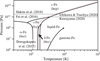 |
Fig. 2 Phase diagram of pure Fe as it is used in the core model of BICEPS. The solid lines are the phase transition curves of Anzellini et al. (2013) and Dorogokupets et al. (2017). The dotted line illustrates the possible shift of the melting curve due to additional FeS in the core, using Eq. (11) to calculate the depression in the melting temperature. |
2.4 Mantle layer model
The constituents of the mantle layer considered in the BICEPS model are the simple oxides of the major refractory elements, that is, SiO2, MgO and FeO. These oxides are the most important rock forming elements found in the solar system, for example they account for ~92% of Earth’s mantle mass (Workman & Hart 2005). However, there are other common rock forming elements such as CaO, Al2O3 or NaO2, which were considered in the mantle model used in D17. Regarding the BICEPS model, we neglect their presence since their impact on the mantle density is low, they are not very abundant and they would add large computational complexity to the mantle model. Also only very little thermodynamic data at high pressures is available for these species. Already the FeO-MgO-SiO2 (FMS) system shows a rich phase diagram with various stable phases, especially at lower pressures, rendering it a challenge to model.
2.4.1 Equations of state in the FeO–MgO–SiO2 system
D15 and D17 used the Perple_X code by Connolly (2009), together with the thermodynamic model of Stixrude & Lithgow-Bertelloni (2011) to calculate the stable minerals at a given pressure, temperature and composition. However, the thermody-namic model of Stixrude & Lithgow-Bertelloni (2011) has two main limitations: First, since it was intended to model mantle minerals under Earth like conditions, it is accurate only in a pressure regime similar to Earth like conditions, second, it does not include molten phases. However, when considering more massive rock dominated exoplanets (with masses >10 mE), the pressures at the core mantle boundary (CMB) can reach orders of TPa (Umemoto et al. 2017), far beyond Earth like conditions4,5. Further, planetary equilibrium temperatures of more than 1000 K, together with a significant volatile layer, already lead to temperatures much larger than the liquidus of rock at the mantle/volatile boundary layer, resulting in partially molten mantle layers (Lopez & Fortney 2014; Dorn & Lichtenberg 2021). Indeed Vazan et al. (2018) argued that most sub-Neptune sized exoplanets with volatile envelopes > 0.02 mE will host a magma ocean below the volatile envelope.
In absence of a general thermodynamic model of the FMS system, which would be valid at pressures up to the TPa regime and which includes solid and liquid phases, we propose the following mantle model. In a first step the P–T space is divided into a solid and a fluid region, where each a different set of EoSs is used. To determine where to switch the two sets of EoSs we use the melting curve of Belonoshko et al. (2005; P < 199.5 GPa) and Stixrude (2014; P ≥ 199.5 GPa) for pure MgSiO3
 (15)
(15)
including a correction for additional MgO, SiO2 or FeO compared to the pure MgSiO3 composition
 (16)
(16)
Throughout both liquid and solid region we assume that the temperature follows an adiabat, thus the temperature gradient is similar to the one in the core
 (17)
(17)
with γ being the Grüneisen parameter and KS the isentropic bulk modulus. Numerical modeling of mantles of Earth like planets and Super-Earths showed, that the thermal profiles in the deep mantle tend to be super adiabatic (Tackley et al. 2013). But since the thermal expansivity of the solid mantle phases at high pressures is very small, the effect of assuming an adiabatic temperature gradient instead of a super adiabatic one is expected to be small.
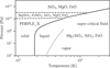 |
Fig. 3 Schematic representation of the considered mantle model. Illustrating the wide range of thermal conditions covered by the used EoS. The fluid and the solid phases are separated by the MgSiO3 melting curve (solid line) of Eq. (16), including a correction factor for additional MgO, SiO2 and FeO. The two dashed lines represent the perovskite/post-perovskite transition (lower) and dissociation pressure (upper). The dotted line illustrates the approximate location of the vapor curve, calculated using M-ANEOS and the parameters for pure SiO2. |
2.4.2 Solid mantle
In the solid region we expand the method of using Perple_X together with Stixrude & Lithgow-Bertelloni (2011) toward larger pressures. As shown in Fig. 3, we divide the solid phase into three regions. The first region (region 1) extends from ambient pressures up to the perovskite (pv)–postperovskite (ppv) transition given by the Clapeyron relation as in Boujibar et al. (2020)
 (18)
(18)
In this region, we use as in D17 the Perple_X code6 by Connolly (2009) together with the thermodynamic model of Stixrude & Lithgow-Bertelloni (2011). The second region (region 2) extends from Ppv/ppv up to the dissociation pressure of ppv. The mineralogy in this region is dominated by ppv (i.e., [Fe,Mg]SiO3). Depending on the composition, some amounts of FeO, MgO and SiO2 can also be present. Because Perple_X together with the thermodynamic model of Stixrude & Lithgow-Bertelloni (2011) starts to give inconsistent results at these conditions, we do not use any more Perple_X to determine the stable mineralization in this region. Rather we define the stable minerals a priori, considering the aforementioned pure SiO2, post-perovskite ([Mg,Fe]SiO3) and wustite ([Mg,Fe]O). The EoS of MgSiO3-ppv is taken from Sakai et al. (2016), while for FeSiO3-ppv we continue using the thermodynamic model of Stixrude & Lithgow-Bertelloni (2011), in absence of a better model. The EoSs of the other minerals are given by Fischer et al. (2011) for FeO, Musella et al. (2019) for MgO and Faik et al. (2018) for SiO2. For a given mantle composition, the relative amount of each mineral is calculated using the stoichiometric relations shown in Appendix B.2.
It is still debated if ppv undergoes further phase transitions before dissociating into the basic oxides (Boujibar et al. 2020; Umemoto et al. 2017; Tsuchiya & Tsuchiya 2011). We follow Tsuchiya & Tsuchiya (2011) and assume that at a pressure of
 (19)
(19)
ppv dissociates into the basic oxides, without additional intermediate phase transitions. The parameters of the Clapeyron relation Eq. (19) are taken from Boujibar et al. (2020). At pressures above the dissociation pressure (region 3), given by Eq. (19), we only consider the basic oxides SiO2, MgO and FeO. The EoS used for the basic oxides are the same as in the second region (Fischer et al. 2011; Faik et al. 2018; Musella et al. 2019).
The various used EoSs in region 2 and region 3 are combined using the additive volume law, which should be sufficient for the scope of this work (Bradley et al. 2018). An overview over all used EoS is shown in Table 1. We later discuss the impact of the proposed mantle model onto the calculated planetary radii.
2.4.3 Liquid mantle
For the liquid mantle we assume that it consists of a combination of SiO2, FeO and Mg2SiO4 (similar to Dorn & Lichtenberg 2021). Forsterite (Mg2SiO4) was chosen instead of MgO, since Stewart et al. (2020) recently published an updated version of the modified analytical equation of state (M-ANEOS) with parameters for Forsterite, which covers consistently a very large range in pressure and temperature. For SiO2 we use the EoS of Faik et al. (2018; except at pressures lower than 20 GPa we use Melosh 2007 since the EoS in Faik et al. 2018 does not properly model the region below the critical point). While for FeO we use the same EoS as in the liquid core, though with parameters for FeO (Ichikawa & Tsuchiya 2020). As the EoS parameters were not provided directly, we fit the EoS parameters from the available data, see Appendix C. Again, the EoSs are combined assuming ideal mixing with the additive volume law.
Overview over all used EoS in the BICEPS model.
2.5 Volatile layer
The outermost layer in the BICEPS structure model is the volatile layer, made up of H, He and H2O. These three species offer a large range of atmosphere compositions which can be modeled, that is, from H, He dominated primary atmospheres to water dominated secondary atmospheres. While other volatile species are most likely present in a planet, we often lack additional information on the atmospheric composition, and sometimes even a proper EoS which covers the needed pressures and temperatures. Thus we constrain BICEPS to consider H, He and H2O for which we have reliable EoS and which are key ingredients in most planetary atmospheres (Nettelmann et al. 2013; Lopez & Fortney 2014; Venturini et al. 2020c).
The incoming stellar flux together with the remaining heat from the planet’s formation have a large impact onto the structure of the volatile layer and the distribution of water within the layer. Thus the volatile layer can be split into three distinct sublayers: an irradiated outer atmosphere (i), an envelope where almost all incoming flux was absorbed in the layer above (ii) and a potential layer of pure H2O below the H/He (iii). The presence of these sublayers depends on the given boundary conditions and the composition of the volatile layer. The model parameters of BICEPS related to the volatile layer are the combined H and He mass mH/He, the water mass  , the internal luminosity of the planet Lint and the planetary equilibrium temperature Teq.
2.5.1 Calculation of the internal luminosity
The volatile layer is heated both from the top, that is, from the host star, as well as from below. The remaining heat of formation and the heat of radiogenic elements are the main sources of an exoplanet’s internal luminosity Lint. As we do not calculate the evolution of the observed exoplanet over its full history, but rather look at a static snapshot in the exoplanet’s history, we calculate the internal luminosity using the age–luminosity relation presented in Mordasini (2020).
This relation estimates the intrinsic luminosity Lint of an exoplanet given its mass, age and composition. Lint is thus calculated using
 (20)
(20)
where the parameters a0, b1, b2, c1 and c2 depend on the planets age7 and are given in Table A.1 of Mordasini (2020). Further quantities are mCore, mMantle,  , LJ, that is, the mass of the planet’s iron core, rocky mantle, water content, hydrogen and helium content and the luminosity of Jupiter respectively. The fit of Mordasini (2020) was made from a series of planetary evolution calculations for planets with a total mass of 1 mE ≤ mtot ≤ 40 mE. The simulations include the contribution of the cooling and contraction of the core, mantle and envelope, together with the radiogenic luminosity from a chondritic abundance of radionucleides (Mordasini et al. 2012). The simulations of Mordasini (2020) were performed for a limited set of compositions. Indeed it would be preferential to have a fit based on a wider range of compositions. But the planets luminosity is most sensitive to the planets age, while the composition is a second order effect, as shown in Fig. A.2 of Mordasini (2020).
Using this description of the internal luminosity allows us to simplify the calculation of Eq. (4) to
 (21)
(21)
as L = Lint is calculated for the whole planet at once.
2.5.2 Irradiated atmosphere
The stellar flux is deposited in the outermost sublayer of the volatile layer, which we call the irradiated atmosphere. The temperature structure within the irradiated atmosphere is calculated using the non-gray analytical atmosphere model of Parmentier & Guillot (2014) and Parmentier et al. (2015). From Parmentier et al. (2015) we use in particular the parameters of model D, which is a fit to radiative transfer models of solar composition atmospheres. We also use their fit of the Bond albedo AB for solar composition atmospheres, from the same publication.
In order to evaluate model D, the effective temperature of the atmosphere needs to be calculated first. Given Tint and Teq we calculate the zero albedo effective temperature
 (22)
(22)
Here Tint is the temperature associated with the heat flux from the interior
 (23)
(23)
σ is the Stefan-Boltzmann constant, Teq the planetary equilibrium temperature and f is the same scaling parameter of the incoming flux as already used in, for example, Guillot (2010). The variable f is thus 1/2 for the day-side average and 1/4 for an average over the whole planet. Next, the Bond albedo AB is calculated given  and the set of equations in Table 2 of Parmentier et al. (2015). This allows us to then calculate
 (24)
(24)
Given the effective temperature the parameters for model D are calculated. Then we calculate the derivative from Eq. (98) from Parmentier & Guillot (2014) in respect of the optical depth τ, that is,
![Mathematical equation: $\matrix{ {{{\partial T} \over {\partial \tau }} = {1 \over {4 \cdot {T^3}}}\left[ {{3 \over 4}T_{{\rm{int}}}^4\,\left( {1 - {B \over {{\tau _{{\rm{lim}}}}}}{{\rm{e}}^{ - \tau /{\tau _{{\rm{lim}}}}}}} \right)} \right.} \hfill \cr {\,\,\,\,\,\,\,\,\,\,\,\,\left. { + \mathop {\mathop \sum \nolimits^ }\limits_3^{i = 1} 3 \cdot {\beta _{{{\rm{v}}_i}}} \cdot T_{{\rm{eq}}}^4 \cdot {\mu _ * }\,\left( { - {{{D_i}} \over {{\tau _{\lim }}}}{{\rm{e}}^{ - \tau /{\tau _{{\rm{lim}}}}}} - {E_i} \cdot {\gamma _{{v_i}}} \cdot {{\rm{e}}^{ - {\gamma _{{v_i}}}\tau }}} \right)} \right]} \hfill \cr } $](/articles/aa/full_html/2024/01/aa46965-23/aa46965-23-eq29.png) (25)
(25)
and multiply it with
 (26)
(26)
to get the temperature gradient ∇irr in the irradiated atmosphere
 (27)
(27)
The variables of Eqs. (25), that is, τlim, B, Di, Ei,  ,
,  and µ*, are the parameters calculated with model D of Parmentier et al. (2015). In Eq. (26), the variable κ is the gas opacity of the atmosphere, for which we use the Rosseland mean opacity values of Freedman et al. (2014). The density at a given pressure and temperature is calculated using the SCvH-EoS for H/He by Saumon et al. (1995) and the AQUA-EoS for any present H2O (see Sect. 2.5.4). Knowing the temperature gradient and density as a function of pressure and temperature, we can solve the structure Eqs. (1)–(3).
The transition between the irradiated atmosphere layer happens when essentially all stellar flux was absorbed by the atmosphere above, that is, τυ ≫ 1. Determining the exact location is hard when no full radiative transfer calculation is performed. Thus, we tested multiple optical depths and pressures and found that when transitioning at 100 bar, results in smooth transitions along the temperature profile. Note that even at such pressures and large optical depths, model D of Parmentier et al. (2015) is still in agreement with radiative transfer calculations.
Model input and output parameters.
2.5.3 Envelope
The sublayer below the irradiated atmosphere we call the envelope. In the envelope the contribution of the incoming stellar flux to the temperature profile can be neglected, since it was already absorbed in the irradiated atmosphere above. The main difference between the envelope sublayer and the irradiated atmosphere is the calculation of the temperature gradient. In the envelope we use the Ledoux criterion for an ideal gas (Kippenhahn et al. 2012)
 (28)
(28)
to decide if a parcel of gas is in the adiabatic or radiative thermal transport regime. Where the three gradients in Eq. (28) are the radiative temperature gradient
 (29)
(29)
the adiabatic temperature gradient
 (30)
(30)
and the spatial compositional gradient
 (31)
(31)
The variables of Eqs. (29)–(31) are the radiation density constant a, speed of light c, mean opacity κ, luminosity Lint, thermal expansion coefficient α, the specific isobaric heat capacity cP and the mean molecular weight µ. The gradients are calculated using the Rosseland mean opacities by Freedman et al. (2014) while ρ, α, cP and µ are taken again from the SCvH-EoS for H/He by Saumon et al. (1995) and the AQUA-EoS for H2O.
2.5.4 Atmosphere enrichment and water condensation
As already mentioned, BICEPS considers a volatile layer made out of H, He which can be enriched in H2O. As water is one of the main absorbers in the optical wavelengths, its distribution within the volatile layer strongly affects the observed radius of a planet (Baraffe et al. 2008). While enriched envelopes are likely one of the key ingredients for the formation of certain types of planets (i.e., mini-Neptunes Venturini et al. 2015; Venturini & Helled 2017) it remains unknown how strong water will be mixed after Gyrs of a planet’s formation and evolution. Since we do not know a priori how much of a planet’s water is mixed within the envelope, we introduce an additional model parameter fmix ∈ [0,1]. It sets the maximal fraction of the planet’s water which is mixed with the H/He:
 (32)
(32)
The remaining water which is not mixed with the H/He, will form a pure water layer at the bottom of the envelope
 (33)
(33)
But note, that not every combination of Teq, fmix,  and mHHe is physical. When the local temperature within the envelope is below the critical temperature of water and the partial pressure of water is above its vapor pressure, then water will condense and eventually rain out, further altering the distribution of water. Ideally, a global climate model would calculate the many feedbacks related with a planet’s water cycle. But the computational restrictions by the MCMC scheme do not allow for such expensive calculations. We use instead the following simple condensation scheme to account for this effect.
At a given pressure and temperature the H/He gas can only contain a certain amount of water before it is fully saturated and the water would condense and possibly rain out. The H/He gas is saturated when the partial pressure of water is higher than the vapor pressure of water. The partial pressure of water is defined as
 (34)
(34)
where  is the molar fraction of water in the gas, the wi are the mass fractions of the volatile species i, Mi the respective molar masses and Ploc is the local pressure. The vapor pressure is given by the vapor curve (see Wagner et al. 2011). Above the critical point of H2O the H/He gas cannot be saturated any more, and we assume that water is well mixed with H/He under these conditions.
This means that if the atmosphere is always warmer than the critical temperature of water, we assume that the water is uniformly mixed throughout the whole volatile layer. The water mass fraction at each pressure is in this case given by the average water mass fraction mixed in the envelope
 (35)
(35)
If the atmosphere is colder than the critical temperature, we check where potentially condensation could occur. Since the determination of the partial pressure requires to know the local composition of the gas, we need to iterate over the compositional gradient until we find a physical solution. We start by assuming a uniform distribution of water as in Eq. (35). If throughout the volatile layer the condensation criterion is never fulfilled, then the water mass fraction remains constant again as in Eq. (35). Otherwise at any point where the condensation criterion is fulfilled we use the CEA package (Gordon & McBride 1994; McBride & Gordon 1996), to calculate the water mass fraction wsat that can be contained at these conditions. The excess in water Δw which rains out, is then given by
 (36)
(36)
This excess water will be redistributed deeper into the volatile layer increasing  proportional to the mass of the atmosphere layer for which Eq. (36) is evaluated.
At the same time, we need to make sure that the compositional gradient is monotonically increasing with depth, since any decreasing gradient would be dynamically unstable over longer timescales. We therefore also remove water from above the saturated layers until we have a monotonically increasing compositional gradient. This leads to the two possible distribution scenarios depicted in Fig. 4. Either a uniform distribution of H2O throughout the atmosphere (i) or a compositional gradient which shows two concentrations with a sharp transition between them (ii). If we would not remove water above the saturated layers, the method outlined above would lead to a gradient, with a u-shaped drop around the saturated region. Such a configuration would not be stable over time.
If a sufficient amount of water is redistributed, it can happen that at the end of the integration of the structure equations over the mixed layer, some water is left remaining. In this case we add that amount to the pure water layer below.
The EoS used for H2O is the AQUA EoS by Haldemann et al. (2020). The AQUA EoS is a combination of the EoS by Mazevet et al. (2019) with EoS more suitable at low pressures (Gordon & McBride 1994; McBride & Gordon 1996; Wagner & Pruß 2002; Brown 2018) or describing the various ice phases of water (Feistel & Wagner 2006; French & Redmer 2015; Journaux et al. 2020). The EoS of the mixture of H/He and H2O is calculated as in Baraffe et al. (2008).
Note that the presented condensation model is still a basic approximation to the real situation where cloud formation and other dynamical processes would further impact the distribution of water. But it offers the advantage to exclude at least some non-physical cases compared to a model where the water is always uniformly distributed.
2.6 Transit radius
The so-called transit radius is commonly defined to be the radius where the chord optical depth is τch = 2/3 (Guillot 2010). This puts the transit radius often at significant larger radii than the photosphere radius which is defined as the radius where the optical depth in radial direction is τ = 2/3.
The chord optical depth is given by the path integral, along a photon’s path between the stellar photosphere and the observing instrument, with the photon passing through the exoplanet’s envelope
 (37)
(37)
where ds is an infinitesimal element along this path and κv is the wavelength dependent opacity at radius r. Note that the chord optical depth is in its general definition not only a function of radius, but also a function of wavelength v. As proposed in Parmentier & Guillot (2014), we use for κv the Rosseland mean opacity  weighted with the stellar effective temperature
  . The values of
  are taken from Freedman et al. (2014).
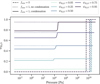 |
Fig. 4 Different compositional gradients in the volatile layer of a 5 mE planet with wVol = 0.4 and water mass fractions in the volatile layer which span from 5% to 95%. Dashed lines: H2O and H/He do not mix. Dotted lines: all of the H2O is mixed into the H/He but without condensation. Solid lines: all of the H2O is mixed into the H/He but condensates are removed as described in Sect. 2.5.4. |
2.7 Thermal boundary layers
We assume that all our planets contain still enough heat from formation to sustain convection within the mantle and the core. This leads to the formation of two thermal boundary layers, one at the core mantle boundary (CMB) and one at the boundary between mantle and volatile layer (MVB). Due to the release of gravitational energy during core formation, the iron core remains likely hotter than the surrounding mantle. Stixrude (2014) argued that the temperature difference at both the CMB and the MVB are governed by the melting temperature of the silicates in the mantle. Following Stixrude (2014) this means that if the temperature just above the CMB or the MVB is lower than the melting temperature of the mantle, we have a temperature jump at the CMB or the MVB up to the melting temperature  of Eq. (16). If the temperature is already above the melting temperature, then there will be no rise in temperature at the CMB or MVB. Given the assumed vigorous convection we neglect the physical extent of the boundary layers. Hence the temperature jump will occur instantaneous at the MVB or the CMB.
As in Stixrude (2014) the temperature difference at the thermal boundary layers can then be written as
 (38)
(38)
and
 (39)
(39)
2.8 Input and output parameters
Before we turn to the statistical part of the model, let us summarize the input and output parameters of the structure model. BICEPS takes as input the total mass of the planet mtot, together with some layer mass fractions. The layer mass fractions are defined as
 (40)
(40)
Since we distinguish between the water and hydrogen helium mass we use wCore,  and wH/He as input parameters while
 (41)
(41)
is calculated internally. In a similar fashion, the composition of each layer is handled. To calculate the composition of the core it is enough to specify xS|Core. xFe|Core can then be calculated using
 (42)
(42)
The mantle composition is similarly given by xFeO|Mantle and  , while
 (43)
(43)
In the volatile layer we assume a solar ratio of H to He, since our opacity tables are calculated for solar composition. Thus the composition of the volatile layer is given by the ratio between  and wH/He. We also define using fmix up to how much water is mixed into the H/He gas. In order to model the effects of the irradiation from the host star, we require the equilibrium temperature of the planet Teq and the effective stellar temperature
  . The internal luminosity of the planet is calculated from the age of the system (see Sect. 2.5.1).
For this set of input parameters, BICEPS calculates the total radius rtot, the thickness of each layer (rCore, rMantle and rVol), as well as the Mg/Si and Si/Fe elemental ratios of the planet. We also save the pressure and temperature at every interface between the model layers. The Mg/Si and Si/Fe values are used in the inverse method to relate the photospheric composition of the host star to the planets bulk composition. A summary of the model input and output parameters is shown in Table 2.
2.9 The inverse method
In order to characterize a planet, we want to know which distribution of the model input parameters explains best some measured data of the planet. Formally, we use Bayesian inference, as in D15 and D17, to compute the posterior probability density functions (pdf) of a set of model parameters m given observed data d and prior information p(m) on m. According to Bayes theorem the pdf of m given d can be computed from
 (44)
(44)
where p(d|m) is called the likelihood function, while p(d) is called Bayes integral or sometimes just the evidence. The likelihood function is a measure of how well the model fits the observed data, while the evidence can be seen as a normalization factor. In BICEPS we mostly represent the likelihood with a multivariate normal distribution
 (45)
(45)
However, depending on the target, other likelihood functions are also possible. Here g(·) is the so-called forward model which calculates, for a set of parameters, the model prediction in the data space. Further,  is the variance of the data in the ith dimension of the data space. We assume that independent measurements are used for the various data parameters, hence the covariance matrix is diagonal.
Depending on the problem, the Bayes integral is often much harder to calculate than the prior or the likelihood. A common solution in order to avoid calculating Bayes integral is to use MCMC methods. MCMC methods are a class of sampling methods, which allow to draw samples from a target distribution p(x), which might be otherwise difficult to be directly sampled. Over the years many different flavors of MCMC algorithms have emerged (Metropolis et al. 1953; Hastings 1970; Geman & Geman 1984; Haario et al. 2001; Foreman-Mackey et al. 2013; Betancourt 2017), including some publicly available implementations: for example emcee8 or JAGS9. For this work we implemented an adaptive Metropolis-Hastings MCMC, which will be shortly introduced in the following subsection. A similar method was already used in D15 and D17.
2.10 Markov chain Monte Carlo method
To calculate the posterior probability p(m|d) of Eq. (44) it is common to use either MCMC sampling (D15; D17; Acuña et al. 2021) or nested sampling methods (Otegi et al. 2020). We follow D17 and use a Metropolis-Hastings MCMC method (Metropolis & Ulam 1949; Metropolis et al. 1953; Hastings 1970), which follows a simple algorithm. Given the ith sample m(i) in the space of model parameters perform the following steps: (i) propose a new point m(p) using the symmetric transition kernel q(m(p)|m(i)), (ii) calculate the prior probability 𝒫(m(p)) of the proposed point and evaluate the likelihood function ℒ(d|m(p), g) given the observed data d and a forward model g(·) which maps m(p) into the space of d, (iii) accept the proposed point with probability
 (46)
(46)
and add it to the Markov chain as (i + 1)th element, otherwise add m(i) to the Markov chain as (i + 1)th element. It was shown in Metropolis et al. (1953), that this algorithm will return samples from a stationary distribution π which is proportional to p(m|d).
It is important to note, that the samples generated from a Markov process such as the one above, are not fully independent, instead they are autocorrelated (Hogg & Foreman-Mackey 2018). The stronger the autocorrelation of the generated samples, the more samples are needed to converge to the desired stationary distribution. In order to have a small autocorrelation, it is important that the Markov chain has a good “mixing”, that is to say that the Markov chain does not remain too long at one point but moves throughout the parameter space. Gelman et al. (1996) showed that for many Metropolis Hastings variants there is an optimal acceptance rate of 0.234, which assures optimal mixing and thus minimizes the autocorrelation. In order to achieve this optimal mixing behavior we periodically tune the proposal distribution q(·|·) according to Haario et al. (2001) and Atchadé & Rosenthal (2005). The numbers of samples necessary until the Markov chain converges to the stationary distribution can only be estimated. The number varies depending on the correlation between subsequent samples and the complexity of the problem. For BICEPS we found that generating ~ 5 × 10⁵ samples is enough, that key statistics such as median, 1-σ intervals, etc. of the marginalized posterior distributions do not change anymore significantly.
Given that the computation of a single planetary structure model takes on the order of seconds to compute, we added another modification to speed up the computation of BICEPS. We leverage the fact that some data variables (i.e., mtot, xSi/xFe|Planet and xMg/xSi|Planet) can be evaluated very fast from the model input parameters. Thus we precompute these parameters with a separate forward model gfast(·). Then we test if the model would be rejected, in the optimal case where the remaining data variables would match the observations. If so we skip the evaluation of the total radius since it would not change the outcome of the acceptance process.
To sample compositional parameters10 on a simplex, we use the self-adjusting logit transform (SALT) proposal by Director et al. (2017) to propose the next move of the Markov chain in this dimension. The MCMC algorithm used in BICEPS is summarized in the scheme of Fig. 5. In order to test the proper behavior of the MCMC implementation we performed a simple validation which is shown in Appendix A.
A strength of the Bayesian inference method is the possibility to include prior information in the inference process. In Table 2, we show an overview over the used model input parameters. For every input parameter we assign a prior distribution. This prior distribution should incorporate the prior knowledge we have about this particular parameter for a given target. For some parameters this information is not known, or we just do not want to favor a particular configuration. In this case, we choose the priors to be as un-informative as possible. For example the composition of the core and the mantle, as well as the layer mass fractions each sum up to one by definition. Hence they each form a probability simplex11. All these parameters are then sampled at uniform density on the respective probability simplex. Due to the used core model in BICEPS, the parameter xS|Core has amaximum value of 0.19. Thus we assign a prior probability of zero to all cases with xS|Core ≥ 0.19.
When inferring a planetary composition, multiple combinations of input parameters can lead to the same predicted planetary radius. Thiabaud et al. (2015) showed that ratios of the refractory elements Mg, Si and Fe of the host star may be a good proxy for the ratios of the bulk planet. Thereafter D17 showed, that including alongside rtot and mtot also xSi/xFe|Planet and xMg/xSi|Planet as data variables, helps reducing the degeneracy of the interior parameters. BICEPS can therefore include xSi/xFe|Planet and xMg/xSi|Planet as data variables, if they are available for a target.
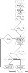 |
Fig. 5 Schematic of the adaptive MCMC algorithm used in BICEPS. |
3 Results
In this section, we show the impact of the planetary structure model described in the previous section onto the radius of a planet with a given mass. We show comparisons for each of the three main layers of the structure model and finally apply the full BICEPS model to characterize the exoplanet TOI-130 b.
3.1 Core layer model comparison
As a first comparison, we solved the structure equations for a pure iron sphere in order to compare our core model against other models used previously. We compare against the EoS of Bouchet et al. (2013), which was used in D17 and the EoS of Hakim et al. (2018). The later case should illustrate the effect of adding the additional Fe-phases (α-Fe, γ-Fe, δ-Fe and liquid Fe) to the planetary core model. For the comparison, we calculated the radii of iron spheres with a range of masses starting at 0.01 mE up to 50 mE. We repeated the calculations for three different boundary conditions at the surface of the iron sphere i) 10 GPa and 1000 K, resembling a small and rather cold mantle layer above the core; ii) 100 GPa and 3000 K, resembling the conditions below an Earth like mantle; iii) 500 GPa and 104 K, resembling a massive and hot mantle layer above the core. The cases (i) and (ii) always result in a solid iron sphere, while in case (iii) the core can be partially to fully molten, depending on the total mass of the sphere. In Fig. 6, we show the relative difference in radius of the iron spheres calculated with the BICEPS core model and the EoS listed before. The relative difference is calculated always with respect to the radius calculated with BICEPS, that is, using
 (49)
(49)
We report that compared to the EoS of Bouchet et al. (2013) the radius of the iron core differs between −2.7% to +2%. Since no liquid Fe model was considered, all radii of case (iii) are smaller than calculated with BICEPS. The kink at around 18 mE is due to the transition of the BICEPS core model from the liquid to the solid phase. In case (ii), the radii are similar up to 3 mE after which the structures calculated with BICEPS are more compressed. In case (i), the differences at masses above 3 mE are the same as in case (ii), but at lower core masses the radii is significantly smaller (down to −2.7%).
The effect of including the fcc phase at low pressures, as well as including a model for liquid iron can be seen in the comparison against the EoS of Hakim et al. (2018). Throughout the pressure range of case (ii) BICEPS only uses the EoS of Hakim et al. (2018), hence the results are identical. Though in case (i) we see the effect of the fcc phase. Which has the biggest effect for very small cores, thought for planets larger than Earth the effect will be small. In contrary to case (iii) where we see an even bigger effect than in the comparison to Bouchet et al. (2013), with a difference in radius of up to 3.2%.
In Fig. 6, we also show the maximum effect of adding sulfur to the core. For this comparison we calculated the relative difference in radius between a core with xS|Core = 0.19 and xS|Core = 0, using the BICEPS core model. For the solid cases, the results are very similar with differences in radii between 1.8% at low core masses and 3.2% at large core masses. For the liquid EoS, the radii are considerably different especially at large core masses, that is, when the EoS is evaluate up to higher pressures. At low core masses the difference in radius is around 2.8%, while it goes up to even 10.5% at 40 mE.
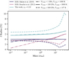 |
Fig. 6 Relative differences when calculating the radius of a pure iron sphere for different EoS. The reference radii are calculated using BICEPS. Dark blue lines: relative radius difference compared to the EoS of Hakim et al. (2018). Pink lines: relative radius difference using the EoS of Bouchet et al. (2013). Light blue lines: relative radius difference when adding to the core the maximum amount of sulfur considered in BICEPS. |
3.2 Mantle layer model comparison
As for the core in the previous section, we perform here a similar model comparison for the mantle. To quantify the difference to D17, we use a mantle model where solely Perple_X and the thermodynamic model of Stixrude & Lithgow-Bertelloni (2011) is used. As a second case we also compare against the mantle model used in Sotin et al. (2007) which considers only four minerals in the mantle, that is, enstatite ([Mg2,Fe2]Si2O6) and olivine ([Mg2,Fe2]Si2O4) in the upper mantle and perovskite ([Mg,Fe]SiO3) and wustite ([Mg,Fe]O) in the lower mantle. For the three models, we compare the radii of pure rocky spheres without any core. The choice of using a pure rocky model is only for the sake of comparing the different models, in reality such exoplanets would likely host a core.
We use three sets of surface boundary conditions, one with Earth-like conditions of PMVB = 1 atm and TMVB = 300 K and two with the same surface pressure as the Earth like case but a temperature above the melting curve of TMVB = 2000 K and TMVB = 2500 K. To also include the effect of composition, we consider three sets of SiO2, FeO, and MgO mantle abundances for each boundary condition. The first composition resembles an Earth-like composition with  , xFeO = 0.058 and xMgO = 0.519. For the two other cases we use compositions with lower Mg to Si abundance ratios, one iron free (
 , xFeO = 0, xMgO = 1/3) and one with a Si to Fe abundance ratio of two (
 , xFeO = 0.25 and xMgO = 0.25). The resulting mantle compositions are also listed in Table 3.
For all of these cases we calculated the radius of these rocky spheres over a range of masses, spanning from 0.01 mE to 20 mE. In Fig. 7, we show the relative difference in radii of the calculated rocky spheres. Note that when comparing against Perple_X and the thermodynamic database of Stixrude & Lithgow-Bertelloni (2011), only spheres up to 10 mE could be calculated, since at higher pressures the Gibbs minimization scheme did not always converge onto a stable mineralization. But even at this masses the sampled pressures exceed the range for which the thermo-dynamic database of Stixrude & Lithgow-Bertelloni (2011) was intended.
When comparing the resulting radii calculated with solely using Perple_X against the radii calculated with the mantle model of BICEPS, one can see that the largest differences appear for the two high temperature boundary conditions up to 1 mE. This is due to the impact of the liquid phases used in the mantle model of BICEPS. Over all compositions the differences are below 2%. Nevertheless one sees that toward higher masses the differences in radii start to diverge again. Since for this comparison low surface pressures were used, it is likely that when the mantle is under a considerable volatile layer, the difference seen here, at large masses, will shift toward smaller mantle masses.
The simple EoSs which are used in Sotin et al. (2007) allowed to evaluate the mantle model over a larger pressure range than when using Perple_X. Similar to the case of Perple_X, we see a large variability in the observed radius differences. Over all compositions the differences range from −5.5% to +1% and are rarely in agreement to Perple_X or the mantle model used in BICEPS. The best agreement is found for the Earth like composition where the relative difference is often less than 1% and very similar to the Perple_X model. For composition C2, which contains the most iron of all three tested compositions, the differences are largest. It seems that using the model of Sotin et al. (2007) to characterize exoplanets is only justified when assuming Earth like compositions and low mantle temperatures.
Mantle compositions for mantle model comparison.
3.3 Volatile layer model comparison
As for the mantle and the core, we show in this section the effect of the BICEPS volatile layer model on the calculation of the planetary radius. Since there are many effects to compare, we split the comparison into four parts: one regarding the used atmosphere irradiation model, one regarding the used water equation of state, one regarding the condensation model and one testing the sensitivity of the luminosity-age relation.
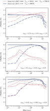 |
Fig. 7 Relative radius difference between pure rocky spheres calculated with different EoS and different mineral compositions. The reference model is the one presented in this work. All cases have the boundary conditions 1 bar and either 300 K (solid lines), 2000 K (dashed lines) or 2500 K (dot dashed lines). |
3.3.1 Atmosphere model
In Fig. 8, we show the comparison between the atmosphere structure calculated using model D of Parmentier et al. (2015) against the atmosphere model used in D17, that is, the atmosphere model presented in Jin et al. (2014). The atmosphere structures are calculated for a 5 mE planet at various equilibrium temperatures. One can see, that the non-gray atmosphere model used in BICEPS predicts a temperature inversion around 0.1 bar for low equilibrium temperatures (Teq ≤ 100 K), while the model of Jin et al. (2014) remains isothermal. Besides the temperature inversions, the temperature profiles appear to be shifted especially at lower pressures. This shift will impact the location of the transit radius, which occurs typically at these lower pressures.
In Fig. 9, the difference in transit radii between the two considered atmosphere models varies strongly with the equilibrium temperature of the exoplanet. The relative difference in transit radius was calculated for six different combinations of exoplanet mass (5 mE and 10 mE) and weight fraction of volatiles (1 wt.%, 0.1 wt.% and 0.001 wt.%). The relative difference in transit radius was calculated using
![Mathematical equation: $\delta {{\rm{R}}_{{\rm{transit}}}}[{\rm{\% }}] = 100 \cdot {{{r_{{\rm{Jin}}}} - {r_{{\rm{BICEPS}}}}} \over {{r_{{\rm{BICEPS}}}}}},$](/articles/aa/full_html/2024/01/aa46965-23/aa46965-23-eq75.png) (50)
(50)
where rJin is the transit radius calculated with the model of Jin et al. (2014) and rBICEPS is the transit radius calculated using the BICEPS model. For this comparison the volatile layer was solely made out of H and He. At increasing exoplanet mass, the results for the different H/He mass fractions get more and more similar, thus for 20 mE only the wvol = 10−2 case is shown. The amplitude of the differences varies between −5% and +5% for equilibrium temperatures below 1400 K. At higher equilibrium temperatures the differences start to diverge. For the case of the lightest considered exoplanet with the most H/He, the difference becomes 10% and more.
Another key factor is the determination of the transit radius itself. As in D17 the transit radius in BICEPS is calculated from the mean opacities of the gas in the volatile layer. Other authors set the transit radius at a fixed pressure (Lopez & Fortney 2014). One can see in Fig. 10 that depending if the transit radius is calculated from the chord optical depth or simply taken at a fixed pressure, has a significant impact on the location of the transit radius. This effect is enhanced toward higher equilibrium temperatures of the exoplanet, for which the outer atmosphere becomes more extended.
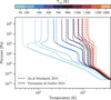 |
Fig. 8 Thermal structure of the volatile layer of a 5 mE exoplanet with 1 wt% of H/He, for various equilibrium temperatures. The coldest equilibrium temperature Teq was chosen to be 50 K, then from Teq = 100 K a profile was calculated every 200 K until Teq = 1500 K. Solid lines: the structure calculated using model D by Parmentier & Guillot (2014). Dashed lines: the atmosphere structure calculated using the model of Jin et al. (2014), which is also used in D17. |
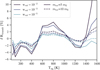 |
Fig. 9 Relative difference in transit radius between the model of Jin et al. (2014) and model D of Parmentier & Guillot (2014) used in BICEPS, as a function of planetary equilibrium temperature. The relative difference was calculated as in Eq. (50) for three different planetary volatile mass fractions of 10−2 (dark blue), 10−3 (blue) and 10−5 (light blue) and two exoplanet masses: 5 mE (solid) and 10 mE (dashed). |
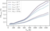 |
Fig. 10 Relative difference in transit radius as a function of equilibrium temperature using different methods calculating the transit radius. The reference transit radius is calculated at τchord = 2/3, which is compared as in Eq. (50) to the transit radius fixed at 20 mbar (see, e.g., Lopez & Fortney 2014). The same cases as in Fig. 9 are considered. |
3.3.2 Liquid water equation of state
In Fig. 11, we show the impact of choosing a different water EoS when calculating the radius of an exoplanet of given composition. For this comparison we calculated the radius of a water dominated exoplanet made out of 50 wt.% H2O, 30 wt.% Mg2SiO4 and 20 wt.% Fe, over a wide range of exoplanet masses (from 0.01 mE to 50 mE). We then calculated the radius of such exoplanets for four different outer boundary temperatures Tout given a particular water EoS. The boundary pressure Pout was chosen at the pressure of the vapor curve for the corresponding temperature
 (51)
(51)
The thermal gradient in the water layer was chosen to be adiabatic. The EoS used for this comparison were the AQUA EoS (Haldemann et al. 2020) as used in this work, the quotidian equation of state (QEOS) of Vazan et al. (2013) as used in D17 and the analytical equation of state (ANEOS) by Melosh (2007) using parameters for water as in Mordasini (2020), which is another often used EoS for water in planetary science. For all cases we used the mantle and core model of BICEPS in order to calculate the layers below the water layer in the same fashion.
In Fig. 11, we show the relative differences in terms of planetary radius between the different EoS. To calculate the relative difference, the same approach as in Eq. (50) was used, thus QEOS and ANEOS are compared against the reference radii calculated using AQUA.
The comparison between AQUA and QEOS shows that for Tout < 500 K, the relative difference in radius is between -5% and 10%. For higher boundary temperatures the radii calculated with QEOS can be more than 20% smaller for small water layers.
When using ANEOS instead of AQUA, the water layers are less dense for Tout < 300 K. As in the case for QEOS the radii are vastly different at higher outer boundary temperatures. In both cases the amplitude of the relative differences decreases toward larger water layers, converging around 5%. Nevertheless the relative differences over the range of considered masses and conditions due to the choice of EoS is very large. Note that this is in line with the results of Haldemann et al. (2020), where a similar comparison for isothermal water layers was performed.
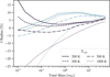 |
Fig. 11 Relative difference in radii of water dominated exoplanets (50 wt.% H2O, 30 wt.% Mg2SiO4, 20 wt.% Fe) using different water EoS. The light blue lines show the relative difference between QEOS (Vazan et al. 2013) and AQUA (Haldemann et al. 2020), while the blue lines show the relative difference between ANEOS (Melosh 2007) and AQUA. The results are shown for four different outer boundary temperatures, while the outer boundary pressure is equal to the pressure of the vapor curve at the corresponding boundary temperature. |
3.3.3 Water condensation model
Next, we compare the effect of the simple water condensation model used in BICEPS to distribute water within the volatile layer. In Fig. 12, we show the relative difference in radius comparing the two cases with or without using the water condensation model for a 5 mE exoplanet with 40 wt.% volatile composition. One can clearly see, that the condensation model only impacts exoplanets with low equilibrium temperature. This was expected since as soon as the local temperature in the volatile layer is always above the critical temperature of water, no further condensation occurs, as the surrounding gas will not become saturated any more.
There is also a clear correlation between the relative difference in the transit radius and the relative amount of water in the volatile layer. Increasing the water mass fraction also enhances the effect of the condensation model. As an example the relative difference in radius, at a water mass fraction of 4 wt.%, is on the order of -2% to +2%. Though for a water dominated volatile layer with a water mass fraction of 36 wt.% the usage of the condensation model results in a up to 10% larger exoplanet.
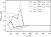 |
Fig. 12 Effect of the condensation model on the transit radius of an exoplanet, shown as the relative difference in radius as a function of Teq. Calculated for an exoplanet of 5 mE, made up of 22 wt.% Fe, 38 wt.% MgSiO3 |Mantle and 40 wt.% volatiles, and for three different volatile layer compositions, i.e., |


3.3.4 Age-luminosity relation
In this paragraph, we show the outcome of a sensitivity analysis of the age-luminosity relation of Mordasini (2020) used to calculate Lint as in Eq. (20). For the analysis, we varied each of the variables used in Eq. (20) by +100%, +10%, -10% and -50% and calculated for various ages, the luminosity of a 10 mE exoplanet made out of 22 wt.% Fe (core), 38 wt.% MgSiO3 (mantle), 10 wt.% (H2O) and 40 wt.% (H/He). We then used BICEPS to calculate the radius of the exoplanet, with a fixed equilibrium temperature of 300 K and also setting ƒmix = 0. The range of considered ages spanned from 0.1 Gyr to 10 Gyr. In Fig. 13, we show the relative difference in the transit radius compared to the case when using the unchanged Eq. (20).
One can see in Fig. 13, that the transit radius of the calculated exoplanets is almost not affected by the value of a0, b1 and c2. Even if the values of the parameters are doubled or halved, the transit radius does not change more than ±1%. Of the five parameters, the age-luminosity relation is most sensitive to the value of c1 and b2. But even for these two variables, when the change is between ± 10%, the relative difference for b2 is always smaller than ±1%, and for c1 always smaller than ±1.5%. Further one can see that the overall sensitivity of all parameters gets reduced with increasing the age of the exoplanet. The reason is that at young ages the luminosities are orders of magnitude larger than at old ages. Thus altering the age-luminosity relation by a given factor, has a much larger effect on the luminosity at young ages (and hence on the exoplanet’s radius) than at old ages.
In comparison, the radius of the modeled exoplanets of this analysis are at 1 Gyr on average 25% smaller than at 0.1 Gyr, while at 10 Gyr they are even 35% smaller. This shows that while Eq. (20) depends on an exoplanet’s composition, for the determination of the luminosity and hence the exoplanet’s radius, the composition is only of secondary importance.
Key parameters of TOI-130b and its host star, based on Sozzetti et al. (2021).
3.4 Characterization of TOI-130 b
In order to showcase the developed model we ran the full BICEPS method for the exoplanet TOI-130b (Sozzetti et al. 2021). For comparison we also ran the same case with the original model used in D17 and compared the outcome of the two inference methods. The observed properties of the star TOI-130 and the detected planet TOI-130 b are given in Table 4.
3.4.1 Setup
Before we can start with the inference method, some parameters need to be determined and the prior and likelihood function need to be chosen. The used data for this comparison are the mass, radius and equilibrium temperature of TOI-130b, the xSi/xFe|Star and xMg/xSi|Star abundance ratios of the host star. Following the arguments in D17, Thiabaud et al. (2015), and Adibekyan et al. (2021) that the abundance ratios of these refractory elements are likely the same or similar between the exoplanet and its host star, we use these abundance ratios to better constrain the possible planetary compositions. Note that this assumption that the host star composition in terms of refractory elements resembles the planetary composition is still debated, (see, e.g., Carter et al. 2015; Plotnykov & Valencia 2020; Adibekyan et al. 2021).
The abundances of these three refractory elements in the photosphere were determined in Sozzetti et al. (2021). These abundances are commonly reported as differences in the decimal exponent (dex) in respect to the solar composition. Thus, in order to calculate xSi/xFe|Planet and xMg/xSi|Planet one can use the following approach: Given the values from Lodders et al. (2009) for the solar reference abundances ALodders [dex] and their standard deviation σLodders [dex] as well as the observed abundances of TOI-130, one can draw multiple times from the random variables:
![Mathematical equation: $\matrix{ {{{\log }_{10}}{x_{{\rm{Si}}}} \sim \left( {{A_{{\rm{Lodders}}}}({\rm{Si}}),{\sigma _{{\rm{Lodders}}}}({\rm{Si}})} \right)} \hfill \cr {\,\,\,\,\,\,\,\,\,\,\,\,\,\,\,\,\,\,\,\,\,\, + \left( {{{[{\rm{Si}}/{\rm{H}}]}_{{\rm{TOI - 130}}}},{\sigma _{{\rm{TOI - 130}}}}({\rm{Si}})} \right),} \hfill \cr } $](/articles/aa/full_html/2024/01/aa46965-23/aa46965-23-eq84.png) (52)
(52)
![Mathematical equation: $\matrix{ {{{\log }_{10}}{x_{{\rm{Mg}}}} \sim \left( {{A_{{\rm{Lodders}}}}({\rm{Mg}}),{\sigma _{{\rm{Lodders}}}}({\rm{Mg}})} \right)} \hfill \cr {\,\,\,\,\,\,\,\,\,\,\,\,\,\,\,\,\,\,\,\,\,\,\,\, + \left( {{{[{\rm{Mg}}/{\rm{H}}]}_{{\rm{TOI - 130}}}},{\sigma _{{\rm{TOI - }}130}}({\rm{Mg}})} \right),} \hfill \cr } $](/articles/aa/full_html/2024/01/aa46965-23/aa46965-23-eq85.png) (53)
(53)
![Mathematical equation: $\matrix{ {{{\log }_{10}}{x_{{\rm{Fe}}}} \sim \left( {{A_{{\rm{Lodders}}}}({\rm{Fe}}),{\sigma _{{\rm{Lodders}}}}({\rm{Fe}})} \right)} \hfill \cr {\,\,\,\,\,\,\,\,\,\,\,\,\,\,\,\,\,\,\,\,\,\,\, + \left( {{{[{\rm{Fe}}/{\rm{H}}]}_{{\rm{TOI}} - 130}},{\sigma _{{\rm{TOI}} - 130}}({\rm{Fe}})} \right)\,.} \hfill \cr } $](/articles/aa/full_html/2024/01/aa46965-23/aa46965-23-eq86.png) (54)
(54)
Here ℕ(μ,σ) is the univariate normal distribution of mean µ and standard deviation σ. This allows to calculate quantiles of the resulting distribution, such as the median Mdn(·) of the abundance ratios, that is,
 (55)
(55)
and
 (56)
(56)
In a similar way also the 1-sigma interval can be calculated. This gives us the distribution of the model variables based on the observed data: xSi/xFe|Planet = 1.15 ± 0.27 and xSi/xFe|Planet = 1.02 ± 0.27.
Since the orbital semi-major axis is already very accurately determined, we do not vary the equilibrium temperature and set it to Teq = 943 K. This leaves us with four observed data variables [mtot, rtot, xSi/xFe|Planet, xMg/xFe|Planet]. We assume that the observed data can be represented by a four dimensional multivariate normal distribution, with mean µobs and covariance matrix Σobs and that the data variables are uncorrelated (see, e.g., Crida et al. 2018, for a case with correlated data variables). The likelihood function is then the one given in Eq. (45) with k = 4. The prior distribution of the model input parameters are listed in Table 5.
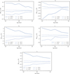 |
Fig. 13 Sensitivity analysis of the age-luminosity relation by Mordasini (2020). Each variable in the fit of Eq. (20) was varied by +100% (solid line), +10% (dotted), −10% (dot dashed) and −50% (dashed). For each case, the transit radius of a 10 mE exoplanet made out of 22 wt.% Fe (core), 38 wt.% MgSiO3 (mantle), 10 wt.% (H2O) and 40 wt.% (H/He) was calculated. The boundary condition was set to be Teq = 300 K and Pout = 1 Pa. In each panel the relative difference to the transit radius calculated with the unchanged Eq. (20) is shown. |
Used prior distribution for TOI-130 b.
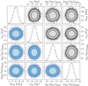 |
Fig. 14 Corner plot of the posterior distribution of the data variables of TOI-130 b. In blue are shown the posteriors generated using BICEPS, while in black are shown the posteriors generated using the original model of D17. For the 2D pair wise marginalized posterior distributions the 68%-HDR (light shaded) and the 89%-HDR (dark shaded) are shown. |
3.4.2 Comparison with Dorn et al. (2017)
The Markov chains for both models were then generated using the MCMC sampler of BICEPS. The MCMC sampler ran until it generated 5000 times more samples than the auto correlation time τƒ ≈ 60 of the data variables (i.e., 3 · 105 samples for each of the two models). In Fig. 14, we show the corner plot of the two posterior distributions over the data variables. The results in blue in this section are always generated using BICEPS while the results in black are generated using the original version of the structure model from D17. One can see that both posterior distributions seem to have converged onto the same target distribution.
In Fig. 15, we then show the corner plot of the posterior distribution for a selection of the model input/output parameters. For readability we forgo to plot all model parameters in a single corner plot, the key statistics of all parameters are instead listed in Table D.1. The 1D marginalized histograms in Fig. 15 show that there is a clear difference for the mass fraction of the mantle, water and H/He layers as well as the pressure at the MVB. In the case of the structure model of D17 a bimodal distribution in the water mass fraction can be seen. Also the BICEPS model has a slight bimodal distribution, but it is much less pronounced than the one using (D17). The reason for this bimodal distribution is related to the chosen EoS of water. The QEOS used in D17 has a strong change in the adiabatic gradient between 1 g cm−3 and 2 g cm−3 even at temperatures larger than the critical temperature. Depending if the condition at the outer boundary of the pure water layer is above or below this abrupt change in the adiabatic temperature gradient, the water layer will have a considerable different density structure. While this change in adiabatic temperature gradient is also present in the AQUA EoS used in BICEPS, it is much smaller compared to QEOS.
Instead of the pairwise scatter plots, one can also show the distribution of the compositional variables directly on a simplex. In Fig. 16 we show both the ternary diagram of the layer mass fractions as well as the ternary diagram of the mantle composition. Note that since the simplex of the layer mass fractions is four dimensional, we combined  and wH/He into
  . The white solid lines in the ternary diagrams indicate contours of the 68%-Highest density region (HDR) and 95%-HDR of the posterior distribution generated using BICEPS. The dashed white lines indicate the same contours for the posteriors generated with the model of D17. The colored background always corresponds to the posterior density of the BICEPS model. We report that the posterior distribution of the mantle composition is almost identical (Fig. 16a), while the posterior distribution of the layer mass fractions shows considerable differences especially at low core mass fractions (Fig. 16b).
We report that for the layer mass fractions, the relative difference in the median increases going from the core (-15%), to the mantle (−13%) to the volatile layer (water: 25%, H/He: ~ 550%), see Table D.1. A similar trend is also seen in the median of the pressure and temperatures at the layer boundaries. As for the median, the 1-σ intervals show differences of a similar pattern. In the case of the 2-σ intervals overall smaller differences can be seen, except for the temperatures at the layer boundaries which change similar to the 1-σ intervals.
In summary, while there are overall considerable differences between the two methods, it is important to note that this is a single result for a particular exoplanet. When characterizing other exoplanets, the differences can be very different. Regarding specifically the case of TOI-130 b, one can state that the posterior distributions generated with BICEPS indicate a more water rich planet (+25% difference in the median) with a smaller core (−15% difference in the median) and smaller mantle (−13% difference in the median). Other compositional variables, such as the mantle composition, are unaffected by the choice of structure model. A notable difference appears in the marginalized distribution of the water mass fraction and the pressure at the mantle water boundary: the original model of D17 results in a strongly bimodal distribution, as explained above.
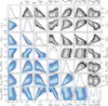 |
Fig. 15 Corner plot of the posterior distribution of some interior structure model variables for TOI-130 b. In blue are shown the posteriors generated using BICEPS, while in black are shown the posteriors generated using the original model of D17. For the 2D pair wise marginalized posterior distributions the 68%-HDR (light shaded) and the 89%-HDR (dark shaded) are shown. |
4 Discussion
4.1 Composition of TOI-130 b
TOI-130 b is a sub-Neptune lying in the second peak of the bimodal size distribution of exoplanets (Fulton et al. 2017). Planets of this type present an intrinsic compositional degeneracy: both a rocky core surrounded by a H-He atmosphere and a water-rich planet can account for the mass and radius.
We used BICEPS to study the possible compositions of TOI-130 b allowing for the presence of a water layer. We found that the water mass fraction is highly unconstrained, and could have all possible ranges. Dry solutions are possible, and in this case, the H-He mass fraction would have an upper limit of ~ 2.5 × 10⁻³ (Fig. 15). This is a very small amount of gaseous atmosphere, but which is very extended due to the high equilibrium temperature of 945 K. TOI-130 b is not a typical sub-Neptune in the sense that it is closer to its star (period of 14 days) than the mean of sub-Neptunes (periods of ~40 days, Martinez et al. 2019). This means that H-He is more prone to be lost by photoevaporation compared to typical sub-Neptunes. Indeed, the maximum fraction of H-He that we find for TOI-130 b could be too low to be retained according to classical evaporation models (Owen & Wu 2017, their Fig. 1), although evaporation models should be computed for this specific planet to gain further constraints.
From a formation point of view, sub-Neptunes are expected to originate beyond the ice line (Venturini et al. 2020b), and hence be water-rich, with typical ice-to-rock ratios of 1:1 (Venturini et al. 2020a). For TOI-130 b, cases with such ice-to-rock ratio would correspond to a planet having a negligible median H-He mass fraction of ~10−8.
Lifting the compositional degeneracy for TOI-130 b will be possible with the determination of atmospheric abundances. This planet would indeed be an excellent candidate for atmospheric characterization with the James Webb Space Telescope (Sozzetti et al. 2021).
TOI-130 b was also characterized in Sozzetti et al. (2021) using a slightly different method than described in this work (see Mortier et al. 2020). They calculated the posterior probability using a four layered structured as done in this work and one scenario without a H/He envelope. They inferred for the scenario with H/He envelope that TOI-130 b would be water rich, with a core mass fraction of  , a mantle mass fraction of
  , a water mass fraction of
  and a H2/He atmosphere mass fraction of
  . The layer mass fractions of wcore, wrock and
  are similar to the results we showed in this work, when running the EoS used in D17, but inferring a much more massive atmosphere. Compared to BICEPS the inferred H/He is also much larger, while the water mass fraction is inferred to be smaller, compensated by a larger core and mantle. The reason for the inferred larger H2/He atmosphere mass fraction in Sozzetti et al. (2021) is most likely twofold, first the atmosphere radius was calculated as in Lopez & Fortney (2014) which provide a fit of the atmosphere radii based on models which have a lowermost H/He mass fraction of 0.001%, second the H/He layer does not affect the temperature/pressure conditions at the transition to the water layer which can affect the radius of the underlying water layer. The differences in the other layer mass fractions are harder to explain as Mortier et al. (2020) used a mixture of EoS (priv. comm.), some EoS are used in BICEPS (e.g., the AQUA-EoS of H2O), while the mantle was calculated as in Sotin et al. (2007). One would have to perform a separate analysis for the particular set of EoS to find the cause of the differences. This problem of exactly attributing differences in the inference of planetary compositions is discussed in the following section.
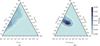 |
Fig. 16 Kernel density estimates (KDE) of the posterior probability distribution of compositional parameters of TOI-130 b inferred using BICEPS. The KDEs were calculated using a Gaussian Kernel with standard deviation of 0.2. Panel a: KDE of the layer mass fractions of TOI-130 b. Panel b: KDE of the mantle composition of TOI-130 b. White solid lines: indicate the contours of the 68%-HDR and 95%-HDR. White dashed lines: indicate the 68%-HDR and 95%-HDR of the posterior distribution calculated with the original model of D17. |
4.2 A general note on BICEPS
In the preceding sections, we introduced the physical models used in BICEPS and performed a model comparison for the major features of the planetary structure model. For most of these comparisons we calculated the relative radius difference for a particular test case, while varying the boundary conditions. These comparisons illustrate the impact various components of the physical model can have on the calculation of the planetary radius. As the differences occur in many different parts of the model, it is unlikely that all of these effects occur at the same time when using BICEPS. Depending on the composition, the mass of the exoplanet and its host star, some aspects will have a bigger impact than others. However, it is nearly impossible to make a priori general statements regarding which effect will have the most significant impact.
We also need to emphasize that BICEPS and any other currently used model to infer planetary compositions includes many simplifying assumptions. Any characterization method has to balance the physical complexity of the internal structure model with the numerical complexity, as the inference should be performed in a useful time. Thus it is necessary to not always choose the best physical description, for example, one could use global climate models, combined with a chemistry model to calculate the distribution of water in the volatile layer. But any such complex model would strongly increase the numerical complexity and make it not feasible to perform an inference in a useful time frame. There are other more conceptual simplifications, such as the choice of having three main layers (core, mantle, volatile layer). While BICEPS is able to model the absence of any of these three main layers, it is possible that some exoplanets have for example a mixed ice and rock layer (Vazan et al. 2022), or a silicate vapor atmosphere (Kite et al. 2016).
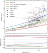 |
Fig. 17 Mass radius diagram and isocomposition curves calculated with BICEPS (solid lines) or taken from Zeng et al. (2019; dashed lines). The boundary conditions are set as in Zeng et al. (2019) to 300 K and 1 mbar. The Earth like composition corresponds to a two layer structure of 32.5 wt% of Fe and 67.5 wt% of MgSiO3. The data for the background exoplanets were taken from the NASA Exoplanet Archive (downloaded the 17.02.2022). Bottom panel: Relative difference between the shown isocomposition curves in the top panel. |
4.3 On the interpretation of a planet's water content
Recently a series of authors studied how water and rock interact under high pressure and temperatures in the interiors of super-Earths and mini-Neptunes. Vazan et al. (2022) concluded that the total water content of a planet cannot be inferred from the atmospheric mass and abundance alone, as a large fraction of the water may be stored in the interior where it is mixed with the rock. Similarly Dorn & Lichtenberg (2021) found that the molten silicates in the mantle can contain a large fraction of water. These considerations affect the interpretation of the water mass fraction w¾o. The parameter w¾o as used in BICEPS describes the mass fraction of water in the surface reservoir only.
4.4 An updated mass radius diagram
In Fig. 17, we show a mass radius diagram with over plotted isocomposition curves. In the background all confirmed exoplanets with an accuracy in mass and radius better than 50% are shown. This kind of mass radius diagram is often used when reporting the detection of an exoplanet, since it gives a fast indication about the possible planetary composition and how common an exoplanet is. As BICEPS has all the necessary ingredients to calculate such isocomposition curves, we provide with this work a set of publicly available isocomposition curves12, calculated for the compositions listed in Table 6.
Besides the isocomposition curves of BICEPS we show in Fig. 17 for comparison the often used isocomposition curves of Zeng et al. (2019). To generate the isocomposition curves with BICEPS the same boundary conditions as in Zeng et al. (2019) were used. For the case of a pure water composition Zeng et al. (2019) provides multiple curves for various surface temperatures, for better readability we only compare the case of 300 K. In the bottom panel of Fig. 17, we also show the relative difference in radius compared to the radius calculated by Zeng et al. (2019). We report that the biggest differences are seen for the pure Fe case, where BICEPS has in average a 6% smaller radius. Both cases which contain rock are generally less dense as the results of Zeng et al. (2019), with radius differences between −0.5% and −2%. The radii of the pure water spheres are in agreement up to 1 mE, afterward the radius difference increases toward 2%.
5 Conclusions
In this work we have presented the BICEPS model, which incorporates recent developments in high pressure equations of state and thereby provides a strong tool to characterize the interiors of intermediate-mass exoplanets. BICEPS combines an internal structure model for exoplanets with an adaptive Metropolis-Hastings method, to calculate the posterior probability distribution of planetary structure parameters. The main features of BICEPS are as follows:
robust internal structure calculations for planets between 0.5 mE and 30 mE,
a non-gray analytical atmosphere model of the irradiated atmospheres,
an updated set of equations of state, spanning a large range in pressure and temperature (including equations of state to model a molten mantle and/or a molten core), and
an adaptive Metropolis-Hastings method capable of efficiently sampling compositional variables.
We compared each part of the internal structure model of BICEPS to other commonly used structure models. Even though the relative differences in radius due to the changes in the core or mantle descriptions are on the order of a few percent, the changes in the description of the volatile layer can be on the order of 10%. The choice of the water equation of state does indeed have a large impact on the calculated radius of water-rich planets. For a particular planet, these effects might not be cumulative but instead be of varying importance depending on the planet’s composition, mass, and equilibrium temperature. We showed with the example of TOI-130 b the magnitude of the effect of using BICEPS, compared to using the original model of D17. We demonstrated that for this particular case BICEPS predicts a more water-rich planet (+25% in the median of the water mass) with a smaller core (–15% in the median of the core mass). For planets of a different mean density and/or different insolation, these results might change.
Our work shows the importance of continuously improving the used internal structure models used to characterize exoplanets. However, even with up-to-date equations of state, and with a robust model of the planetary interior and accurate measurements of the planets' mean density, the intrinsic degeneracies in terms of planetary composition are very hard to overcome. This is mostly due to the large uncertainty related to the composition and structure of the volatile layer. Namely, depending on whether there is a compositional gradient in the volatile layer or not, the radius of the volatile layer differs substantially. It is therefore of great importance to gain further insight into the possible structures and composition of planetary atmospheres, both from a theoretical and observational point of view.
As a final note, we highlight that early versions of the internal structure model of BICEPS were already used to characterize various exoplanets that were observed with CHEOPS, TESS, and ground-based facilities; for more details, readers can refer to K2-111 b (Mortier et al. 2020), TOI-130 b (Sozzetti et al. 2021), TOI-178 b-g (Leleu et al. 2021), TOI-824 b (Burt et al. 2020), TOI-1064 b (Wilson et al. 2022), ν2-Lupi d (Delrez et al. 2021), and L98-59 b (Demangeon et al. 2021), for example. To fully leverage the possibilities of these observational facilities, BICEPS provides a robust structure inference method applicable to a wide range of planet types.
Available iso-composition curves to generate mass radius diagrams.
Acknowledgements
We thank Klaus Mosegaard for this recommendations to improve the MCMC sampling. We also thank the anonymous referee for their comments to improve this manuscript. J.H. and Y.A. acknowledge the support from the Swiss National Science Foundation under grant 200020_172746. J.H. acknowledges the support from the Swiss National Science Foundation under grant 200021_204847 ‘PlanetsInTime’. C.D. acknowledges support from the Swiss National Science Foundation under grant TMSGI2_211313. This work has been carried out within the framework of the NCCR PlanetS supported by the Swiss National Science Foundation under grants 51NF40_182901 and 51NF40_205606. For this publication, the following software packages have been used: Python-lmfit (https://zenodo.org/doi/18.5281/zenodo.598352) by Newville et al. (2014), Python-matplotlib (https://matplotlib.org/) by Hunter (2007), Python-seaborn (https://seaborn.pydata.org/) by Waskom & the seaborn development team (2020), Python-corner (https://corner.readthedocs.io) by Foreman-Mackey (2016), Python-ternary (https://zenodo.org/record/2628066) by Harper et al. (2019), Python-numpy (https://numpy.org/), Python-pandas (https://pandas.pydata.org/).
Appendix A MCMC validation
To validate the MCMC method discussed above, we performed two basic tests as proposed in Hogg & Foreman-Mackey (2018). In the first test we directly sampled several prior distributions with the MCMC method. To do so the likelihood function returned unity for any input it got, therefore the posterior distribution as given by Bayes rule in Eq. (44) should always be equal to the prior distribution. In Fig. A.1 we show an uniformly sampled 3D probability simplex, after the MCMC method sampled 105 points directly from an uniform distribution on the simplex. In Fig. A.2 we show the pdf of four 1D priors sampled by our MCMC (blue) and over plotted the analytical prediction (black). For illustrative purposes we added the top panel of Fig. A.2. It shows a common problem of basic Metropolis Hastings MCMCs, where the pdf of the sampled prior drops close to the domain boundary. This behavior is caused by the fact, that the probability of a move closer toward the domain boundary decreases, the closer the chain is to the boundary. To avoid this issue we choose to use continuous domains for all variables on a compact support, connecting the domain borders such that the chain can move freely across them. As shown in the second panel of Fig. A.2 we do not see this effect for continuous domains.
As a second test we sampled a three dimensional multivariate normal distribution ℕ3(µ, Σ) with mean µ and covariance Σ, arbitrarily set to
![Mathematical equation: ${\bf{\mu }} = \left[ {\matrix{ {0.1} \cr { - 1.0} \cr { - 0.13} \cr } } \right]\,,\quad {\bf{\Sigma }} = \left[ {\matrix{ {1.0} & {0.1} & {0.0} \cr {0.1} & {0.1} & {0.1} \cr {0.0} & {0.1} & {0.2} \cr } } \right]\,.$](/articles/aa/full_html/2024/01/aa46965-23/aa46965-23-eq102.png) (A.1)
(A.1)
In Fig. A.3 we show the results obtained with 106 points given uniform priors in the domain [-3,3] for the model variables x1, x2 and x3. We show in black the analytical predictions over the results of the MCMC in blue. One can see that the MCMC converged to the analytical solution in all three dimensions.
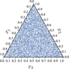 |
Fig. A.1 Results of the first MCMC validation test, where the MCMC sampled directly from the prior distribution. Uniform sampling of a compositional variable on the simplex ∆2. |
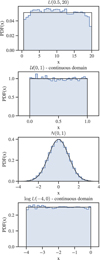 |
Fig. A.2 Results of the first MCMC validation test, where the MCMC sampled directly from the prior distribution. The pdf of the resulting posterior distributions of a run of 105 points for various priors are shown in blue, while the analytical prediction are shown in black. |
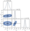 |
Fig. A.3 Corner plot of the second MCMC validation test. The multivariate normal distribution with mean and covariance matrix given in Eq. (A.1), was sampled with 106 points. In black we show the analytical predictions, while in blue we show the results of the MCMC. |
Appendix B Stoichiometric relations
When calculating the internal structure of an exoplanet, a number of stoichiometric relations are needed. In this section we derived the key stoichiometric relations which are used in the BICEPS model. As in the rest of the work wi denotes the mass fraction of species i, while xi denotes the molar fraction of species i. Further, the molar mass of a species is written as Mi, while the number of particles of said species is given by Ni. One can relate the mass and mole fractions using the following two equations
 (B.1)
(B.1)
and
 (B.2)
(B.2)
Where the sum in the calculation of the average molar mass M goes over all species of the considered sample.
B.1 Core composition
The core layer in BICEPS consists of Fe and S, which form the four end members: solid Fe, solid FeS, liquid Fe and liquid Fe081 S019. From the elemental core composition [xFe, xS] the phase composition of [ ,
,  ] for the solid phase and [
 ,
,  ] for the liquid phase can be calculated. The composition of the solid phase is calculated using the following relations:
 (B.3)
(B.3)
To calculate the phase composition of the liquid phase, we first consider that 81 iron atoms per 19 sulfur atoms are needed to form Fe081 S019. Therefore, the number of iron atoms not bound to a sulfur atom are given by
 (B.4)
(B.4)
while the number of Fe081 S019 is simply given by
 (B.5)
(B.5)
The phase composition is then calculated by dividing  and
and  by the sum of
  and
and  , that is,
 (B.6)
(B.6)
Since the number of iron and sulfur atoms in the core are proportional to the molar fraction of the corresponding atom, that is,
 (B.7)
(B.7)
one can simplify Eq. (B.6), which results in
 (B.8)
(B.8)
Because of the choice of liquid EoS used in the core layer, an upper limit of xS < 0.19 on the maximal amount of sulfur has to be imposed on what cases can be modeled with the BICEPS model.
B.2 Mantle composition
The mantle layer in BICEPS is split into four distinct sublayers. For two of them stoichiometric relations are needed to calculate the phase composition.
B.2.1 Lower mantle
The lower mantle layer in the BICEPS consist of Fe, Mg, Si and O, which form the solid end members FeO, MgO, SiO2, MgSiO3 and FeSiO3. From the elemental mantle composition [xFeO, xMgO,  ] the phase composition of [
 ,
,  ,
,  ,
,  ,
,  ] can be calculated. We define first the magnesium number,
 (B.9)
(B.9)
If  we assume that all SiO2 is contained in the post-perovskite phases MgSiO3 and FeSiO3. The relative amount of the end members of post-perovskite is given by the magnesium number, hence one can write:
If  :
:
 (B.10)
 (B.11)
 (B.12)
 (B.13)
 (B.14)
 (B.15)
 (B.16)
 (B.17)
 (B.18)
 (B.19)
 (B.20)
 (B.21)
B.2.2 Liquid mantle
The liquid mantle layer in the BICEPS consist of Fe, Mg, Si and O, which form the liquid end members FeO, Mg2SiO4 and SiO2. From the elemental mantle composition [xFeO, xMgO,  ] the phase composition of [
 ,
,  ,
,  ] can be calculated. The composition of the liquid mantle is calculated using the following relations:
 (B.22)
 (B.23)
 (B.24)
and
 (B.25)
 (B.26)
 (B.27)
Due to the fact that the only magnesium bearing phase in the liquid mantle is Mg2SiO4 an additional constraint arises. The BICEPS mantle model requires that  . As MgO and SiO2 only appear in the mantle layer of BICEPS, the planetary Mg to Si ratio is equal to the ratio in the mantle. Thus if we assume that the ratios of refractory elements in the photosphere of the host star are equal to the one in the planet, this constraint affects the possible targets for which BICEPS can be used. Fortunately most FGK-stars have NMg/NSi ratios below two (Hinkel et al. 2014).
Appendix C Determining EoS parameters for FeO
In the liquid mantle we use the EoS of Ichikawa & Tsuchiya (2020) for liquid FeO. Ichikawa & Tsuchiya (2020) provide the P-V-T data including best fit values for the Mie-Grüneisen EoS combined with a cold Vinet EoS, for various mixtures of Fe, S, O, Ni and Si. Though for FeO only the P-V-T data, but no best fit values of the eight EoS parameters are provided. Hence we refit it from the data provided in Fig. S1 of the supplementary material of Ichikawa & Tsuchiya (2020), using the lmfit-python package (Newville et al. 2014). To reduce the number of free parameters we kept the values of the EoS parameters V0 = 1.51·10−5 m3/mol, γ0 = 1.5, a = 0.0 and b = 1.0 constant, as it was also done for the other mixtures in Ichikawa & Tsuchiya (2020). Using the method of least squares and 35 P-V-T data points, the best fit values of  GPa,
GPa,  , e0 = 0.077 J/mol, and g = −0.139 were determined. In Fig. C.1 the best fit values were used to calculate the volume of FeO as a function of pressure and temperature and compare it against the data of Ichikawa & Tsuchiya (2020).
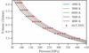 |
Fig. C.1 Volume of liquid FeO as a function of pressure and temperature calculated using the best fit values (solid lines) and compared against the values (red points) taken from Ichikawa & Tsuchiya (2020). |
Appendix D Summary statistics for TOI-130 b
In Table D.1, we summarize the statistical characteristics of the posterior pdf calculated using BICEPS and using the model of D17. For each variable and each model we calculated the median, the boundaries of the centered 1-σ intervals (which contain 68% of all samples) and the centered 2-σ intervals (which contain 95% of all samples) of the 1D marginalized posterior distributions. Further we also calculated the relative difference between the interval boundaries of each variable when calculated using BICEPS or using D17:
![Mathematical equation: $\left[ {{\rm{\Delta }}{A_1},{\rm{\Delta }}{A_2}} \right] = \left[ {100{{A_1^{{\rm{Dorn }} + 17} - A_1^{{\rm{BICEPS }}}} \over {A_1^{{\rm{BICEPS }}}}},100{{A_2^{{\rm{Dorn }} + 17} - A_2^{{\rm{BICEPS }}}} \over {A_2^{{\rm{BICEPS }}}}}} \right]$](/articles/aa/full_html/2024/01/aa46965-23/aa46965-23-eq153.png) (D.1)
(D.1)
where A1, A2 are the interval boundaries.
Statistics of the ID marginalized posterior distribution of all model variables and the relative differences between the distribution generated with BICEPS and the one based on the method of D17.
References
- Acuña, L., Deleuil, M., Mousis, O., et al. 2021, A & A, 647, A53 [CrossRef] [EDP Sciences] [Google Scholar]
- Adibekyan, V., Dorn, C., Sousa, S. G., et al. 2021, Science, 374, 330 [NASA ADS] [CrossRef] [Google Scholar]
- Aitchison, J. 1982, J. Roy. Stat. Soc. Ser. B (Methodological), 44, 139 [Google Scholar]
- Anzellini, S., Dewaele, A., Mezouar, M., Loubeyre, P., & Morard, G. 2013, Science, 340, 464 [NASA ADS] [CrossRef] [Google Scholar]
- Atchadé, Y. F., & Rosenthal, J. S. 2005, Bernoulli, 11, 815 [Google Scholar]
- Baraffe, I., Chabrier, G., & Barman, T. 2008, A & A, 482, 315 [NASA ADS] [CrossRef] [EDP Sciences] [Google Scholar]
- Baumeister, P., Padovan, S., Tosi, N., et al. 2020, ApJ, 889, 42 [Google Scholar]
- Bazhanova, Z. G., Roizen, V. V., & Oganov, A. R. 2017, Physics-Uspekhi, 60, 1025 [NASA ADS] [CrossRef] [Google Scholar]
- Belonoshko, A. B., Skorodumova, N. V., Rosengren, A., et al. 2005, Phys. Rev. Lett., 94, 195701 [CrossRef] [Google Scholar]
- Benneke, B., & Seager, S. 2012, ApJ, 753, 100 [NASA ADS] [CrossRef] [Google Scholar]
- Benz, W., Broeg, C., Fortier, A., et al. 2021, Exp. Astron., 51, 109 [Google Scholar]
- Betancourt, M. 2017, arXiv e-prints [arXiv: 1701.02434] [Google Scholar]
- Bouchet, J., Mazevet, S., Morard, G., Guyot, F., & Musella, R. 2013, Phys. Rev. B, 87, 094102 [Google Scholar]
- Boujibar, A., Driscoll, P., & Fei, Y. 2020, J. Geophys. Res.: Planets, 125, e2019JE006124 [CrossRef] [Google Scholar]
- Bradley, P. A., Loomis, E. N., Merritt, E. C., et al. 2018, Phys. Plasmas, 25, 012710 [CrossRef] [Google Scholar]
- Brown, J. M. 2018, Fluid Phase Equilibria, 463, 18 [CrossRef] [Google Scholar]
- Burt, J. A., Nielsen, L. D., Quinn, S. N., et al. 2020, AJ, 160, 153 [Google Scholar]
- Carter, P. J., Leinhardt, Z. M., Elliott, T., Walter, M. J., & Stewart, S. T. 2015, ApJ, 813, 72 [NASA ADS] [CrossRef] [Google Scholar]
- Chubb, K. L., Min, M., Kawashima, Y., Helling, C., & Waldmann, I. 2020, A & A, 639, A3 [NASA ADS] [CrossRef] [EDP Sciences] [Google Scholar]
- Connolly, J. A. D. 2009, Geochem. Geophys. Geosyst., 10, Q10014 [Google Scholar]
- Crida, A., Ligi, R., Dorn, C., & Lebreton, Y. 2018, ApJ, 860, 122 [NASA ADS] [CrossRef] [Google Scholar]
- Delrez, L., Ehrenreich, D., Alibert, Y., et al. 2021, Nat. Astron., 5, 775 [NASA ADS] [CrossRef] [Google Scholar]
- Demangeon, O. D. S., Zapatero Osorio, M. R., Alibert, Y., et al. 2021, A & A, 653, A41 [CrossRef] [EDP Sciences] [Google Scholar]
- Director, H. M., Gattiker, J., Lawrence, E., & Wiel, S. V. 2017, J. Stat. Comput. Simul., 87, 3521 [CrossRef] [Google Scholar]
- Dorn, C., & Lichtenberg, T. 2021, ApJ, 922, L4 [NASA ADS] [CrossRef] [Google Scholar]
- Dorn, C., Khan, A., Heng, K., et al. 2015, A & A, 577, A83 [NASA ADS] [CrossRef] [EDP Sciences] [Google Scholar]
- Dorn, C., Venturini, J., Khan, A., et al. 2017, A & A, 597, A37 [NASA ADS] [CrossRef] [EDP Sciences] [Google Scholar]
- Dorogokupets, P. I., Dymshits, A. M., Litasov, K. D., & Sokolova, T. S. 2017, Sci. Rep., 7, 41863 [NASA ADS] [CrossRef] [Google Scholar]
- Dziewonski, A. M. & Anderson, D. L. 1981, Phys. Earth Planet. Interiors, 25, 297 [CrossRef] [Google Scholar]
- Faik, S., Tauschwitz, A., & Iosilevskiy, I. 2018, Comput. Phys. Commun., 227, 117 [NASA ADS] [CrossRef] [Google Scholar]
- Fei, Y., Murphy, C., Shibazaki, Y., Shahar, A., & Huang, H. 2016, Geophys. Res. Lett., 43, 6837 [NASA ADS] [CrossRef] [Google Scholar]
- Feistel, R., & Wagner, W. 2006, J. Phys. Chem. Ref. Data, 35, 1021 [NASA ADS] [CrossRef] [Google Scholar]
- Fischer, R. A., Campbell, A. J., Shofner, G. A., et al. 2011, Earth Planet. Sci. Lett., 304, 496 [CrossRef] [Google Scholar]
- Foreman-Mackey, D. 2016, J. Open Source Softw., 1, 24 [Google Scholar]
- Foreman-Mackey, D., Hogg, D. W., Lang, D., & Goodman, J. 2013, PASP, 125, 306 [Google Scholar]
- Freedman, R. S., Lustig-Yaeger, J., Fortney, J. J., et al. 2014, ApJS, 214, 25 [CrossRef] [Google Scholar]
- French, M., & Redmer, R. 2015, Phys. Rev. B, 91, 014308 [CrossRef] [Google Scholar]
- Fulton, B. J., Petigura, E. A., Howard, A. W., et al. 2017, AJ, 154, 109 [Google Scholar]
- Gelman, A., Roberts, G. O., & Gilks, W. R. 1996, in Proceedings of the Fifth Valencia International Meeting Bayesian Statistics (Valencia: Oxford University Press), 599 [CrossRef] [Google Scholar]
- Geman, S., & Geman, D. 1984, IEEE Trans. Pattern Anal. Mach. Intell., PAMI-6, 721 [CrossRef] [Google Scholar]
- Gordon, S., & McBride, B. J. 1994, Computer Program for Calculation of Complex Chemical Equilibrium Compositions and Applications. Part 1: Analysis, Tech. rep., NASA Lewis Research Center [Google Scholar]
- Guillot, T. 2010, A & A, 520, A27 [NASA ADS] [CrossRef] [EDP Sciences] [Google Scholar]
- Haario, H., Saksman, E., & Tamminen, J. 2001, Bernoulli, 7, 223 [CrossRef] [Google Scholar]
- Hakim, K., Rivoldini, A., Van Hoolst, T., et al. 2018, Icarus, 313, 61 [Google Scholar]
- Haldemann, J. 2021, PhD thesis, Universität Bern, Switzerland [Google Scholar]
- Haldemann, J., Alibert, Y., Mordasini, C., & Benz, W. 2020, A & A, 643, A105 [NASA ADS] [CrossRef] [EDP Sciences] [Google Scholar]
- Haldemann, J., Ksoll, V., Walter, D., et al. 2023, A & A, 672, A180 [NASA ADS] [CrossRef] [EDP Sciences] [Google Scholar]
- Harper, M., Weinstein, B., Simon, C., et al. 2019, https://doi.org/18.5281/zenodo.2628066 [Google Scholar]
- Hastings, W. K. 1970, Biometrika, 57, 97 [Google Scholar]
- Hinkel, N. R., Timmes, F. X., Young, P. A., Pagano, M. D., & Turnbull, M. C. 2014, AJ, 148, 54 [NASA ADS] [CrossRef] [Google Scholar]
- Hogg, D. W., & Foreman-Mackey, D. 2018, ApJS, 236, 11 [NASA ADS] [CrossRef] [Google Scholar]
- Huang, C., Rice, D. R., & Steffen, J. H. 2022, MNRAS, 513, 5256 [NASA ADS] [CrossRef] [Google Scholar]
- Hunter, J. D. 2007, Comput. Sci. Eng., 9, 90 [NASA ADS] [CrossRef] [Google Scholar]
- Ichikawa, H., & Tsuchiya, T. 2020, Minerals, 10, 59 [CrossRef] [Google Scholar]
- Jin, S., Mordasini, C., Parmentier, V., et al. 2014, ApJ, 795, 65 [Google Scholar]
- Journaux, B., Brown, J. M., Pakhomova, A., et al. 2020, J. Geophys. Res.: Planets, 125, e2019JE006176 [CrossRef] [Google Scholar]
- Khalafinejad, S., Molaverdikhani, K., Blecic, J., et al. 2021, A & A, 656, A142 [NASA ADS] [CrossRef] [EDP Sciences] [Google Scholar]
- Kippenhahn, R., Weigert, A., & Weiss, A. 2012, Stellar Structure and Evolution, 2nd edn., Astronomy & Astrophysics Library (Berlin Heidelberg: SpringerVerlag) [Google Scholar]
- Kite, E. S., Fegley, Bruce, J., Schaefer, L., & Gaidos, E. 2016, ApJ, 828, 80 [NASA ADS] [CrossRef] [Google Scholar]
- Kuwayama, Y., Morard, G., Nakajima, Y., et al. 2020, Phys. Rev. Lett., 124, 165701 [NASA ADS] [CrossRef] [Google Scholar]
- Leleu, A., Alibert, Y., Hara, N. C., et al. 2021, A & A, 649, A26 [NASA ADS] [CrossRef] [EDP Sciences] [Google Scholar]
- Lodders, K., Palme, H., & Gail, H.-P. 2009, in Solar System, 4B, eds. W. Martienssen, & J. Trümper, (Berlin, Heidelberg: Springer Berlin Heidelberg), 712 [CrossRef] [Google Scholar]
- Lopez, E. D., & Fortney, J. J. 2014, ApJ, 792, 1 [Google Scholar]
- Martinez, C. F., Cunha, K., Ghezzi, L., & Smith, V. V. 2019, ApJ, 875, 29 [Google Scholar]
- Mayor, M., Pepe, F., Queloz, D., et al. 2003, The Messenger, 114, 20 [NASA ADS] [Google Scholar]
- Mazevet, S., Licari, A., Chabrier, G., & Potekhin, A. Y. 2019, A & A, 621, A128 [NASA ADS] [CrossRef] [EDP Sciences] [Google Scholar]
- McBride, B. J., & Gordon, S. 1996, Computer Program for Calculation of Complex Chemical Equilibrium Compositions and Applications II. Users Manual and Program Description, Tech. rep., NASA Lewis Research Center [Google Scholar]
- Melosh, H. J. 2007, Meteor. Planet. Sci., 42, 2079 [NASA ADS] [CrossRef] [Google Scholar]
- Metropolis, N., & Ulam, S. 1949, J. Am. Stat. Assoc., 44, 335 [Google Scholar]
- Metropolis, N., Rosenbluth, A. W., Rosenbluth, M. N., Teller, A. H., & Teller, E. 1953, J. Chem. Phys., 21, 1087 [Google Scholar]
- Mordasini, C. 2020, A & A, 638, A52 [NASA ADS] [CrossRef] [EDP Sciences] [Google Scholar]
- Mordasini, C., Alibert, Y., Klahr, H., & Henning, T. 2012, A & A, 547, A111 [NASA ADS] [CrossRef] [EDP Sciences] [Google Scholar]
- Mortier, A., Zapatero Osorio, M. R., Malavolta, L., et al. 2020, MNRAS, 499, 5004 [Google Scholar]
- Musella, R., Mazevet, S., & Guyot, F. 2019, Phys. Rev. B, 99, 064110 [NASA ADS] [CrossRef] [Google Scholar]
- Nettelmann, N., Helled, R., Fortney, J. J., & Redmer, R. 2013, Planet. Space Sci., 77, 143 [Google Scholar]
- Newville, M., Stensitzki, T., Allen, D. B., & Ingargiola, A. 2014, https://doi.org/10.5281/zenodo.11813 [Google Scholar]
- Noack, L., & Lasbleis, M. 2020, A & A, 638, A129 [NASA ADS] [CrossRef] [EDP Sciences] [Google Scholar]
- Otegi, J. F., Dorn, C., Helled, R., et al. 2020, A & A, 640, A135 [NASA ADS] [CrossRef] [EDP Sciences] [Google Scholar]
- Owen, J. E., & Wu, Y. 2017, ApJ, 847, 29 [Google Scholar]
- Parmentier, V., & Guillot, T. 2014, A & A, 562, A133 [NASA ADS] [CrossRef] [EDP Sciences] [Google Scholar]
- Parmentier, V., Guillot, T., Fortney, J. J., & Marley, M. S. 2015, A & A, 574, A35 [NASA ADS] [CrossRef] [EDP Sciences] [Google Scholar]
- Pepe, F., Molaro, P., Cristiani, S., et al. 2014, Astron. Nachr., 335, 8 [Google Scholar]
- Plotnykov, M., & Valencia, D. 2020, MNRAS, 499, 932 [CrossRef] [Google Scholar]
- Press, W. H., Teukolsky, S. A., Vetterling, W. T., & Flannery, B. P. 1996, Numerical Recipes in Fortran 90, 2nd edn.: The Art of Parallel Scientific Computing (New York, NY, USA: Cambridge University Press) [Google Scholar]
- Ricard, Y., Šrámek, O., & Dubuffet, F. 2009, Earth Planet. Sci. Lett., 284, 144 [CrossRef] [Google Scholar]
- Ricker, G. R., Winn, J. N., Vanderspek, R., et al. 2014, J. Astron. Telescopes Instrum. Syst., 1, 014003 [NASA ADS] [CrossRef] [Google Scholar]
- Sakai, T., Dekura, H., & Hirao, N. 2016, Sci. Rep., 6, 1 [CrossRef] [Google Scholar]
- Sata, N., Hirose, K., Shen, G., et al. 2010, J. Geophys. Res.: Solid Earth, 115, B09204 [NASA ADS] [CrossRef] [Google Scholar]
- Saumon, D., Chabrier, G., & van Horn, H. M. 1995, ApJS, 99, 713 [NASA ADS] [CrossRef] [Google Scholar]
- Schulze, J. G., Wang, J., Johnson, J. A., et al. 2021, Planet. Sci. J., 2, 113 [NASA ADS] [CrossRef] [Google Scholar]
- Seager, S., Kuchner, M., Hier-Majumder, C. A., & Militzer, B. 2007, ApJ, 669, 1279 [NASA ADS] [CrossRef] [Google Scholar]
- Sotin, C., Grasset, O., & Mocquet, A. 2007, Icarus, 191, 337 [Google Scholar]
- Sozzetti, A., Damasso, M., Bonomo, A. S., et al. 2021, A & A, 648, A75 [NASA ADS] [CrossRef] [EDP Sciences] [Google Scholar]
- Stewart, S., Davies, E., Duncan, M., et al. 2020, AIP Conf. Proc., 2272, 080003 [NASA ADS] [CrossRef] [Google Scholar]
- Stixrude, L. 2014, Philos. Trans. Roy. Soc. A: Math. Phys. Eng. Sci., 372, 20130076 [NASA ADS] [CrossRef] [Google Scholar]
- Stixrude, L. & Lithgow-Bertelloni, C. 2011, Geophys. J. Int., 184, 1180 [NASA ADS] [CrossRef] [Google Scholar]
- Tackley, P. J., Ammann, M., Brodholt, J. P., Dobson, D. P., & Valencia, D. 2013, Icarus, 225, 50 [NASA ADS] [CrossRef] [Google Scholar]
- Thiabaud, A., Marboeuf, U., Alibert, Y., Leya, I., & Mezger, K. 2015, A & A, 580, A30 [NASA ADS] [CrossRef] [EDP Sciences] [Google Scholar]
- Tsuchiya, T., & Tsuchiya, J. 2011, Proc. Natl. Acad. Sci. U.S.A., 108, 1252 [NASA ADS] [CrossRef] [Google Scholar]
- Umemoto, K., Wentzcovitch, R. M., Wu, S., et al. 2017, Earth Planet. Sci. Lett., 478, 40 [CrossRef] [Google Scholar]
- Unterborn, C. T., & Panero, W. R. 2019, J. Geophys. Res.: Planets, 124, 1704 [NASA ADS] [CrossRef] [Google Scholar]
- Unterborn, C. T., Dismukes, E. E., & Panero, W. R. 2016, ApJ, 819, 32 [Google Scholar]
- Valencia, D., O’Connell, R. J., & Sasselov, D. 2006, Icarus, 181, 545 [Google Scholar]
- Valencia, D., Sasselov, D. D., & O’Connell, R. J. 2007, ApJ, 656, 545 [Google Scholar]
- van den Berg, A. P., Yuen, D. A., Umemoto, K., Jacobs, M. H. G., & Wentzcovitch, R. M. 2019, Icarus, 317, 412 [NASA ADS] [CrossRef] [Google Scholar]
- Vazan, A., Kovetz, A., Podolak, M., & Helled, R. 2013, MNRAS, 434, 3283 [NASA ADS] [CrossRef] [Google Scholar]
- Vazan, A., Ormel, C. W., Noack, L., & Dominik, C. 2018, ApJ, 869, 163 [NASA ADS] [CrossRef] [Google Scholar]
- Vazan, A., Sari, R., & Kessel, R. 2022, ApJ, 926, 150 [NASA ADS] [CrossRef] [Google Scholar]
- Venturini, J., & Helled, R. 2017, ApJ, 848, 95 [NASA ADS] [CrossRef] [Google Scholar]
- Venturini, J., Alibert, Y., Benz, W., & Ikoma, M. 2015, A & A, 576, A114 [NASA ADS] [CrossRef] [EDP Sciences] [Google Scholar]
- Venturini, J., Guilera, O. M., Haldemann, J., Ronco, M. P., & Mordasini, C. 2020a, A & A, 643, A1 [Google Scholar]
- Venturini, J., Guilera, O. M., Ronco, M. P., & Mordasini, C. 2020b, A & A, 644, A174 [NASA ADS] [CrossRef] [EDP Sciences] [Google Scholar]
- Venturini, J., Ronco, M. P., & Guilera, O. M. 2020c, Space Sci. Rev., 216, 86 [NASA ADS] [CrossRef] [Google Scholar]
- Wagner, W., & Pruß, A. 2002, J. Phys. Chem. Ref. Data, 31, 387 [Google Scholar]
- Wagner, W., Riethmann, T., Feistel, R., & Harvey, A. H. 2011, J. Physical Chem. Ref. Data, 40, 043103 [NASA ADS] [CrossRef] [Google Scholar]
- Waskom, M., Gelbart, M., Botvinnik, O., et al. 2020, https://doi.org/10.5281/zenodo.592845 [Google Scholar]
- Wilson, T. G., Goffo, E., Alibert, Y., et al. 2022, MNRAS, 511, 1043 [NASA ADS] [CrossRef] [Google Scholar]
- Workman, R. K., & Hart, S. R. 2005, Earth Planet. Sci. Lett., 231, 53 [CrossRef] [Google Scholar]
- Zeng, L., Jacobsen, S. B., Sasselov, D. D., et al. 2019, PNAS, 116, 9723 [Google Scholar]
- Zhao, Y., & Ni, D. 2021, A & A, 650, A177 [NASA ADS] [CrossRef] [EDP Sciences] [Google Scholar]
It is important to remember that this relation is not unique, since many different compositions can lead to the same mean density.
Throughout this work we use the convention that xi denotes the molar fraction of species i and wi is used for weight fractions.
As defined in Eq. (5), ∇ is the dimensionless temperature gradient, hence ∇Ad has to be written as ∇Ad = γ • P/KS instead of the also commonly used dimensionful quantity γ • T/KS.
We tried extrapolating the thermodynamic model of Stixrude & Lithgow-Bertelloni (2011) to pressures larger than 1 TPa together with using Perple_X, but the equilibrium calculations often resulted in nonphysical phase combinations.
Note that the proposed upper limit of 630 GPa CMB pressure for super-Earths by Unterborn & Panero (2019) is only valid for exoplanets with radii smaller than 1.5 RE respectively ≲5 mE.
Perple_X: version 6.8.9, http://www.perplex.ethz.ch/
Since planet formation takes place during the first few Myr of a stars lifetime (Venturini et al. 2020c), the formation timescale is orders of magnitudes shorter than the estimated lifetime of most host stars (~Gyr), thus the age of the host star is a very good proxy for the age of the planet.
Compositional parameters are parameters which have the supplementary condition that they sum to a constant, that is,
 (47)
(47)
This linear dependence requires special sampling techniques (Aitchison 1982). Compositional parameters for which c = 1 lie on the k-dimensional probability simplex.
The regular (k – 1)-probability-simplex is a polyhedron given by the set of points which fulfill
 (48)
(48)
For example the 2d probability simplex is the equilateral triangle in the 3d space with edges at (1,0,0), (0,1,0) and (0,0,1).
All Tables
Statistics of the ID marginalized posterior distribution of all model variables and the relative differences between the distribution generated with BICEPS and the one based on the method of D17.
All Figures
|
Fig. 1 Schematic representation of the interior structure model. The modeled exoplanet consists of three main layers: an iron core in the center, surrounded by a silicate mantle, below an envelope made out of volatile elements, irradiated by the host star. |
| In the text | |
|
Fig. 2 Phase diagram of pure Fe as it is used in the core model of BICEPS. The solid lines are the phase transition curves of Anzellini et al. (2013) and Dorogokupets et al. (2017). The dotted line illustrates the possible shift of the melting curve due to additional FeS in the core, using Eq. (11) to calculate the depression in the melting temperature. |
| In the text | |
|
Fig. 3 Schematic representation of the considered mantle model. Illustrating the wide range of thermal conditions covered by the used EoS. The fluid and the solid phases are separated by the MgSiO3 melting curve (solid line) of Eq. (16), including a correction factor for additional MgO, SiO2 and FeO. The two dashed lines represent the perovskite/post-perovskite transition (lower) and dissociation pressure (upper). The dotted line illustrates the approximate location of the vapor curve, calculated using M-ANEOS and the parameters for pure SiO2. |
| In the text | |
|
Fig. 4 Different compositional gradients in the volatile layer of a 5 mE planet with wVol = 0.4 and water mass fractions in the volatile layer which span from 5% to 95%. Dashed lines: H2O and H/He do not mix. Dotted lines: all of the H2O is mixed into the H/He but without condensation. Solid lines: all of the H2O is mixed into the H/He but condensates are removed as described in Sect. 2.5.4. |
| In the text | |
|
Fig. 5 Schematic of the adaptive MCMC algorithm used in BICEPS. |
| In the text | |
|
Fig. 6 Relative differences when calculating the radius of a pure iron sphere for different EoS. The reference radii are calculated using BICEPS. Dark blue lines: relative radius difference compared to the EoS of Hakim et al. (2018). Pink lines: relative radius difference using the EoS of Bouchet et al. (2013). Light blue lines: relative radius difference when adding to the core the maximum amount of sulfur considered in BICEPS. |
| In the text | |
|
Fig. 7 Relative radius difference between pure rocky spheres calculated with different EoS and different mineral compositions. The reference model is the one presented in this work. All cases have the boundary conditions 1 bar and either 300 K (solid lines), 2000 K (dashed lines) or 2500 K (dot dashed lines). |
| In the text | |
|
Fig. 8 Thermal structure of the volatile layer of a 5 mE exoplanet with 1 wt% of H/He, for various equilibrium temperatures. The coldest equilibrium temperature Teq was chosen to be 50 K, then from Teq = 100 K a profile was calculated every 200 K until Teq = 1500 K. Solid lines: the structure calculated using model D by Parmentier & Guillot (2014). Dashed lines: the atmosphere structure calculated using the model of Jin et al. (2014), which is also used in D17. |
| In the text | |
|
Fig. 9 Relative difference in transit radius between the model of Jin et al. (2014) and model D of Parmentier & Guillot (2014) used in BICEPS, as a function of planetary equilibrium temperature. The relative difference was calculated as in Eq. (50) for three different planetary volatile mass fractions of 10−2 (dark blue), 10−3 (blue) and 10−5 (light blue) and two exoplanet masses: 5 mE (solid) and 10 mE (dashed). |
| In the text | |
|
Fig. 10 Relative difference in transit radius as a function of equilibrium temperature using different methods calculating the transit radius. The reference transit radius is calculated at τchord = 2/3, which is compared as in Eq. (50) to the transit radius fixed at 20 mbar (see, e.g., Lopez & Fortney 2014). The same cases as in Fig. 9 are considered. |
| In the text | |
|
Fig. 11 Relative difference in radii of water dominated exoplanets (50 wt.% H2O, 30 wt.% Mg2SiO4, 20 wt.% Fe) using different water EoS. The light blue lines show the relative difference between QEOS (Vazan et al. 2013) and AQUA (Haldemann et al. 2020), while the blue lines show the relative difference between ANEOS (Melosh 2007) and AQUA. The results are shown for four different outer boundary temperatures, while the outer boundary pressure is equal to the pressure of the vapor curve at the corresponding boundary temperature. |
| In the text | |
|
Fig. 12 Effect of the condensation model on the transit radius of an exoplanet, shown as the relative difference in radius as a function of Teq. Calculated for an exoplanet of 5 mE, made up of 22 wt.% Fe, 38 wt.% MgSiO3 |Mantle and 40 wt.% volatiles, and for three different volatile layer compositions, i.e., |
| In the text | |
|
Fig. 13 Sensitivity analysis of the age-luminosity relation by Mordasini (2020). Each variable in the fit of Eq. (20) was varied by +100% (solid line), +10% (dotted), −10% (dot dashed) and −50% (dashed). For each case, the transit radius of a 10 mE exoplanet made out of 22 wt.% Fe (core), 38 wt.% MgSiO3 (mantle), 10 wt.% (H2O) and 40 wt.% (H/He) was calculated. The boundary condition was set to be Teq = 300 K and Pout = 1 Pa. In each panel the relative difference to the transit radius calculated with the unchanged Eq. (20) is shown. |
| In the text | |
|
Fig. 14 Corner plot of the posterior distribution of the data variables of TOI-130 b. In blue are shown the posteriors generated using BICEPS, while in black are shown the posteriors generated using the original model of D17. For the 2D pair wise marginalized posterior distributions the 68%-HDR (light shaded) and the 89%-HDR (dark shaded) are shown. |
| In the text | |
|
Fig. 15 Corner plot of the posterior distribution of some interior structure model variables for TOI-130 b. In blue are shown the posteriors generated using BICEPS, while in black are shown the posteriors generated using the original model of D17. For the 2D pair wise marginalized posterior distributions the 68%-HDR (light shaded) and the 89%-HDR (dark shaded) are shown. |
| In the text | |
|
Fig. 16 Kernel density estimates (KDE) of the posterior probability distribution of compositional parameters of TOI-130 b inferred using BICEPS. The KDEs were calculated using a Gaussian Kernel with standard deviation of 0.2. Panel a: KDE of the layer mass fractions of TOI-130 b. Panel b: KDE of the mantle composition of TOI-130 b. White solid lines: indicate the contours of the 68%-HDR and 95%-HDR. White dashed lines: indicate the 68%-HDR and 95%-HDR of the posterior distribution calculated with the original model of D17. |
| In the text | |
|
Fig. 17 Mass radius diagram and isocomposition curves calculated with BICEPS (solid lines) or taken from Zeng et al. (2019; dashed lines). The boundary conditions are set as in Zeng et al. (2019) to 300 K and 1 mbar. The Earth like composition corresponds to a two layer structure of 32.5 wt% of Fe and 67.5 wt% of MgSiO3. The data for the background exoplanets were taken from the NASA Exoplanet Archive (downloaded the 17.02.2022). Bottom panel: Relative difference between the shown isocomposition curves in the top panel. |
| In the text | |
|
Fig. A.1 Results of the first MCMC validation test, where the MCMC sampled directly from the prior distribution. Uniform sampling of a compositional variable on the simplex ∆2. |
| In the text | |
|
Fig. A.2 Results of the first MCMC validation test, where the MCMC sampled directly from the prior distribution. The pdf of the resulting posterior distributions of a run of 105 points for various priors are shown in blue, while the analytical prediction are shown in black. |
| In the text | |
|
Fig. A.3 Corner plot of the second MCMC validation test. The multivariate normal distribution with mean and covariance matrix given in Eq. (A.1), was sampled with 106 points. In black we show the analytical predictions, while in blue we show the results of the MCMC. |
| In the text | |
|
Fig. C.1 Volume of liquid FeO as a function of pressure and temperature calculated using the best fit values (solid lines) and compared against the values (red points) taken from Ichikawa & Tsuchiya (2020). |
| In the text | |
Current usage metrics show cumulative count of Article Views (full-text article views including HTML views, PDF and ePub downloads, according to the available data) and Abstracts Views on Vision4Press platform.
Data correspond to usage on the plateform after 2015. The current usage metrics is available 48-96 hours after online publication and is updated daily on week days.
Initial download of the metrics may take a while.