| Issue |
A&A
Volume 672, April 2023
|
|
|---|---|---|
| Article Number | A180 | |
| Number of page(s) | 16 | |
| Section | Planets and planetary systems | |
| DOI | https://doi.org/10.1051/0004-6361/202243230 | |
| Published online | 20 April 2023 | |
Exoplanet characterization using conditional invertible neural networks
1
Department of Space Research & Planetary Sciences, University of Bern,
Gesellschaftsstrasse 6,
3012
Bern, Switzerland
e-mail: This email address is being protected from spambots. You need JavaScript enabled to view it.
2
Abteilung Physik, Gymnasium Lerbermatt,
Kirchstrasse 64,
3098
Köniz, Switzerland
3
Universität Heidelberg, Zentrum für Astronomie, Institut für Theoretische Astrophysik,
Albert-Ueberle-Straße 2,
69120
Heidelberg, Germany
e-mail: This email address is being protected from spambots. You need JavaScript enabled to view it.
4
Universität Heidelberg, Interdisziplinäres Zentrum für Wissenschaftliches Rechnen,
Im Neuenheimer Feld 205,
69120
Heidelberg, Germany
5
Computer Vision and Learning Lab (HCI, IWR),
Universität Heidelberg Berliner Str. 43,
69120
Heidelberg, Germany
Received:
31
January
2022
Accepted:
20
February
2023
Abstract
Context. The characterization of the interior of an exoplanet is an inverse problem. The solution requires statistical methods such as Bayesian inference. Current methods employ Markov chain Monte Carlo (MCMC) sampling to infer the posterior probability of the planetary structure parameters for a given exoplanet. These methods are time-consuming because they require the evaluation of a planetary structure model ~105 times.
Aims. To speed up the inference process when characterizing an exoplanet, we propose to use conditional invertible neural networks to calculate the posterior probability of the planetary structure parameters.
Methods. Conditional invertible neural networks (cINNs) are a special type of neural network that excels at solving inverse problems. We constructed a cINN following the framework for easily invertible architectures (FreIA). This neural network was then trained on a database of 5.6 × 10⁶ internal structure models to recover the inverse mapping between internal structure parameters and observable features (i.e., planetary mass, planetary radius, and elemental composition of the host star). We also show how observational uncertainties can be accounted for.
Results. The cINN method was compared to a commonly used Metropolis-Hastings MCMC. To do this, we repeated the characterization of the exoplanet K2-111 b, using both the MCMC method and the trained cINN. We show that the inferred posterior probability distributions of the internal structure parameters from both methods are very similar; the largest differences are seen in the exoplanet water content. Thus, cINNs are a possible alternative to the standard time-consuming sampling methods. cINNs allow infering the composition of an exoplanet that is orders of magnitude faster than what is possible using an MCMC method. The computation of a large database of internal structures to train the neural network is still required, however. Because this database is only computed once, we found that using an invertible neural network is more efficient than an MCMC when more than ten exoplanets are characterized using the same neural network.
Key words: planets and satellites: interiors / methods: numerical / methods: data analysis
© The Authors 2023
 Open Access article, published by EDP Sciences, under the terms of the Creative Commons Attribution License (https://creativecommons.org/licenses/by/4.0), which permits unrestricted use, distribution, and reproduction in any medium, provided the original work is properly cited.
This article is published in open access under the Subscribe to Open model. This email address is being protected from spambots. You need JavaScript enabled to view it. to support open access publication.
1 Introduction
More than a decade ago, exoplanetary science has entered the era of characterization, where new observations are used to infer physical and chemical properties of exoplanets. These properties can be related to the atmosphere (e.g., Hoeijmakers et al. 2019; Madhusudhan 2019) or to the planetary composition (e.g., Dorn et al. 2015). In the latter case, mass and radius measurements of an exoplanet are used to derive its internal structure (e.g., size of the iron core, presence of water, or gas mass fraction). This problem is notoriously strongly degenerate (Rogers & Seager 2010), but part of this degeneracy can be removed by assuming that the bulk refractory composition of an exoplanet matches the composition of its parent star (Dorn et al. 2017b). This assumption is supported by numerical simulations (e.g., Thiabaud et al. 2015) as well as Solar System observations (e.g., Sotin et al. 2007), although studies of observed exoplanets are not yet conclusive (Plotnykov & Valencia 2020; Schulze et al. 2021; Adibekyan et al. 2021).
Even under the assumption that the bulk compositions of the exoplanet and parent star match, the problem of deriving the planetary composition from the mass, radius, and refractory composition remains degenerate. The traditional method is to use Bayesian inference where the posterior probability of the planetary structure parameters is derived from the set of observed parameters, given prior probability distributions on the planetary structure parameters. These Bayesian calculations are in general performed using a Markov chain Monte Carlo (MCMC) method (Mosegaard & Tarantola 1995; Dorn et al. 2015; Dorn et al. 2017b; Haldemann et al., in prep.)
Markov chain Monte Carlo methods are an efficient and well-tested way of sampling probability distributions. No analytical description of the whole normalized probability density function (PDF) of the target distribution is required. Instead, only the ratios of the PDF at pairs of locations in the phase space need to be calculated (Hogg & Foreman-Mackey 2018). This means that in the case of Bayesian inference, only the prior probability and the likelihood function need to be computed, and the expensive calculation of Bayes’ integral can be skipped, which acts as a normalization constant. A short conceptual summary of a common Metropolis Hastings MCMC method (Metropolis et al. 1953; Hastings 1970) is shown in Fig. 1. We refer to Trotta (2008) and Hogg & Foreman-Mackey (2018) for a more detailed introduction into MCMC methods and MCMC sampling.
In the past years, MCMC sampling together with a planetary structure model has led to a number of successful planetary characterizations (e.g., Dorn et al. 2017a; Agol et al. 2021), but using an MCMC suffers from at least two main difficulties. The first difficulty is that when planetary parameters are measured with small error bars, the likelihood function becomes very narrow. This is for instance the case for radius determination using high-precision telescopes such as CHEOPS (Benz et al. 2017, 2021) or PLATO in the future (Rauer & Heras 2018). Depending on the MCMC method that was used, small error bars can drastically increase the time required to converge to a solution. The second difficulty lies in the consideration of multiplanetary systems. In planetary systems, the observable data of the individual planets are often correlated. To benefit from these correlations, it is necessary to run an inference scheme for the whole system at once. When multiple exoplanets are characterized simultaneously, however, a planetary structure model needs to be calculated for every considered exoplanet. This increases the computational cost linearly. At the same time, the number of parameters that characterize the planetary compositions in a multiplanetary system is similarly scaled with the number of exoplanets. This increase in dimensionality of the parameter space also generally implies an increase in the number of points needed to properly sample the posterior distribution, and therefore, an increase in the required computing time, which is more than linear overall.
In this paper, we propose a new method to derive the posterior distribution of planetary structure parameters. This method is based on conditional invertible neural networks (cINNs), which are a type of neural network architecture that is able to provide the posterior distribution of planetary structure parameters for any given choice of observed parameters (e.g., mass, radius, and refractory composition of the host star). The cINN has proven to be a robust method for calculating the posterior distribution in an inverse problem for any perfect observation, that is, without observational uncertainty, within the range of the training data (Ardizzone et al. 2019a,b). In this work, we expand the method to observations with observational uncertainties (see Sect. 2). Because the cINN was first proposed for cases without observational uncertainty, it is naturally suited for the case of high-precision measurements with very small uncertainties. Another key aspect is that once it is trained, the cINN provides the posterior distribution of planetary structure parameters in a few minutes, where modern MCMCs often require hours or even days to converge because the evaluation of the forward model is time-consuming (see Sect. 4).
In the past years, several authors used machine learning techniques to predict the output of a forward model (e.g., Alibert & Venturini 2019; Lin et al. 2022), or to solve inverse problems (de Wit et al. 2013; Atkins et al. 2016; Baumeister et al. 2020). The inverse problems were mostly modeled using mixture density neural networks (Bishop 1994), that is, a combination of a deep neural network with a probability mixture model. Likewise, cINNs have already seen successful applications in astronomy. Ksoll et al. (2020) were able to estimate stellar parameters from photometric observations of resolved star clusters using a cINN, and Kang et al. (2022) recently showed a cINN approach to recover physical parameters of star-forming clouds from spectral observations.
This paper is structured in the following way. In Sect. 2 we describe the basic concept of cINNs. We show how they can be set up in order to characterize exoplanets and how the forward model works that generates the training data for the neural networks. In Sect. 3, we first validate our proposed method using a simple toy model. In Sect. 4, we then apply the proposed method to characterize an observed exoplanet and compare its performance to a regular Metropolis-Hastings MCMC that was previously used for the same purpose. In Sect. 5, we discuss the current limitations of the approach and compare the time required to run either an MCMC or use the proposed method for cINNs. Finally, we summarize our findings in Sect. 6.
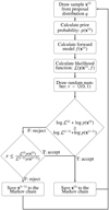 |
Fig. 1 Schematic overview of a Metropolis Hastings MCMC algorithm. The MCMC algorithm generates samples x(0) … x(n) ~ π, where the distribution π is proportional to the posterior probability p(x|y). |
2 Methods
2.1 Invertible neural networks
The invertible neural network (INN) provides an architecture that excels in solving inverse problems (Ardizzone et al. 2019a). In these problems, access to a well-understood forward model is often given (e.g., a simulation) that describes the mapping between underlying physical parameters x of an object and their corresponding observable quantities y, for instance. At the same time, however, recovering the inverse mapping y → x, which is of central interest in many applications, is a difficult task. The INN approach to these inverse problems makes the additional assumption that the known forward model always induces some form of information loss in the mapping of x → y, which can be encoded in some unobservable, latent variables z. Leveraging a fully invertible architecture the INN is then trained to approximate the known forward model f, learning to associate x values with unique pairs of [y, z], that is, a bijective mapping. In doing so, it automatically provides a solution for the inverse mapping f−1 for free. For simplicity (as described in Ardizzone et al. 2019a), it is further assumed that the latent variables z follow a Gaussian prior distribution, which is enforced during the training process. In principle, however, any desired distribution can be prescribed for the latent priors.
Given a new observation y, this procedure allows us to predict the full posterior distribution p(x|y) by simply sampling from the known prior distribution of the latent space. The architecture of the INN consists of a series of reversible blocks, so-called afflne coupling blocks, following a design proposed by Dinh et al. (2016). After splitting the input vector u into two halves u1 and u2, these blocks perform two complementary afflne transformations,
 (1)
(1)
 (2)
(2)
using element-wise multiplication ⊙ and addition. Here, si and ti denote arbitrarily complex mappings of u2 and v1, for example, like small fully connected networks, which are not required to be invertible as they are only ever evaluated in the forward direction.
Inverting these affine transformations is trivial following
 (3)
(3)
 (4)
(4)
2.1.1 Conditional invertible neural networks
We employ a modification to this approach called conditional invertible neural network (cINN), as proposed in Ardizzone et al. (2019b) and as previously applied in Ksoll et al. (2020). Here, the affine coupling blocks are adapted to accept a conditioning input c such that the mappings in Eqs. (1)–(4), that is, s2(u2), t2(u2), and so on, are replaced with s2([u2‚ c]) and t2([u2‚ c]), respectively. By concatenating conditions to the inputs of the subnetworks like this, the invertibility of the architecture is not affected. The forward f(x; c) = z and backward mapping x = g(z; c) of the cINN both entail this conditioning, and the invertibility of the network is given for the fixed condition c as f(·;c)−1 = g(·; c).
When using cINNs for inverse regression problems, such as characterizing the internal structure of an exoplanet, the observations y (e.g., planetary mass, radius, and stellar refractory composition) serve as the conditioning input. Figure 2 shows a schematic representation of the cINN in this case. In doing so, the cINN, just like the INN, will learn to encode all the variance of the physical parameters x that is not explained by the observations y into the latent variables z during training. In addition to usually delivering better results, the cINN approach has the additional advantage that no zero padding is needed if the dimensions of [y, z] and x do not match, as we can simply set dim(z) = dim(x), (Ardizzone et al. 2019a,b). Zero padding refers to a procedure in which a zero vector of dimension k = |m − n| is appended to either the input x or output [y, z] if their dimensions dim(x) = m and dim([y, x]) = n do not match, which is a requirement in the standard INN approach. The zero padding can also be used to embed the entire problem into a higher dimensional space. The latter, however, introduces further hyperparameters and, thus, complicates the training procedure.
Given the condition c of a new observation y, the posterior distribution of the physical parameters is, as for the INN, determined by sampling the latent variables z from their Gaussian prior,
 (5)
(5)
where I is the K × K unity matrix with K = dim(z). In this framework, prior information on x is learned by the network from the distribution of x in the set of training data. This means that the distribution of the training data should follow the prior probability distribution p(x).
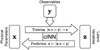 |
Fig. 2 Schematic overview of the cINN. During training, the cINN learns to encode all information about the physical parameters x in the latent variables z (while enforcing that they follow a Gaussian distribution) that is not contained in the observations y. At prediction time, conditioned on the new observation y, the cINN then transforms the known prior distribution p(z) to x-space to retrieve the posterior distribution p(x|y). |
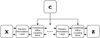 |
Fig. 3 Schematic overview over the cINN architecture. |
2.1.2 Network architecture
For the work presented in this paper, we employed the framework for easily invertible architectures (FrEIA; Ardizzone et al. 2019a,b) and mostly followed the specific cINN architecture suggested in Ardizzone et al. (2019b). This means that we alternated the reversible afflne coupling blocks in the generative flow (GLOW; Kingma & Dhariwal 2018) configuration with random permutation layers (see Fig. 3 for a schematic of the structure). The former is a computationally efficient variant, where the outputs of the mappings si(·) and ti(·) are predicted jointly by a single subnetwork instead of one each. We used simple three-layer (width of 512 per layer) fully connected networks with rectified linear unit (ReLU) activation functions for these subnetworks. The random permutation layers use random orthogonal matrices that were fixed during training and are cheaply invertible, to better mix the information between the streams u1 and u2. Together with the structure of the affine transformations, this ensured that the cINN cannot just ignore the conditioning input during training. In our final architecture, we employed eight reversible blocks (an optimal value that we determined through extensive hyperparameter search for the given problem). In contrast to Ardizzone et al. (2019b), we did not apply a feature extraction network that transforms the input conditions into an intermediate representation because of the low dimensionality of the observable parameter space in our problem. Some early experiments have shown that a network like this did not benefit the predictive performance of the cINN on the given regression task. We trained the cINN by minimizing the maximum likelihood loss ℒ,
![Mathematical equation: ${\cal L} = {{\rm{E}}_i}\left[ {{{\left\| {f\left( {{{\bf{x}}_i};{{\bf{c}}_{\bf{i}}},\theta } \right)} \right\|_2^2} \over 2} - \log \left| {{J_i}} \right|} \right],$](/articles/aa/full_html/2023/04/aa43230-22/aa43230-22-eq6.png) (6)
(6)
where xi, ci denote the parameter-condition pair of training sample i, θ refers to the network weights, and  is the determinant of the Jacobian evaluated at training example i. To update the weights during training, we used the widely used adaptive moment estimation (ADAM) optimizer. For further details, we refer to Ardizzone et al. (2019b).
2.2 Forward model
The forward model f maps the physical input parameters x to a prediction in the data space y′, that is,
 (7)
(7)
It does so by calculating the interior structure of a 1D spherically symmetric sphere in hydrostatic equilibrium. Following Kippenhahn et al. (2012) and similar to the case of stellar structures, we solved the two point boundary value problem given by the equations
 (8)
(8)
 (9)
(9)
 (10)
(10)
where r is the radius, m is the mass within the radius r, P is the pressure, T is the temperature, ρ is the density, G is the gravitational constant, and ∇ is the dimensionless temperature gradient. The sphere was split into three layers of distinct composition similar to a differentiated planet (see Fig. 4). The thermodynamic properties of each layer are given by the set of equations of state (EoS) listed in Table 1.
From the EoS, we calculated ρ, the thermal expansion coefficient α, and the specific heat capacity cP. We assumed that each layer is in a regime of vigorous convection. Therefore, the dimensionless temperature gradient is given by the adiabatic temperature gradient
 (11)
(11)
2.2.1 Core
We considered a solid iron core made out ofhcp-Fe with possible inclusions of less dense FeS alloys. In the model, the composition of the core is given by the sulfur fraction xS|Core, that is,
 (12)
(12)
 (13)
(13)
The thermodynamic properties of Fe and FeS within the core were calculated using the EoS of Hakim et al. (2018). However, for Fe at pressures below 310 GPa, the EoS of Fei et al. (2016) was used, as advised by Hakim et al. (2018).
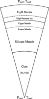 |
Fig. 4 Schematic representation of the layered planetary structure. Three main layers are present: the core, silicate mantle, and volatile layer. Depending on the size of the layers, an upper mantle can be present if the volatile layer above is not too massive. Conversely, if the volatile layer is massive enough, high-pressure ices might form on the bottom of the layer. |
List of EoSs used in the forward model.
2.2.2 Mantle
The mantle structure was calculated following the model used in Sotin et al. (2007). It assumes a homogeneous elemental composition of Fe, Mg, Si, and O throughout the mantle, considering four different minerals. In the upper mantle, the model includes the iron and magnesium end members of the minerals olivine ([Mg,Fe]2SiO4) and ortho pyroxene ([Mg,Fe]2Si2O6), while for the lower mantle, a composition of perovskite ([Mg,Fe]SiO3) and wüstite ([Mg,Fe]O) is assumed. The transition between upper and lower mantle was calculated as in Sotin et al. (2007),
 (14)
(14)
The respective fractions of the upper and lower mantle mineral phases were calculated from the ratios of the xMg/xSi|Mantle and xFe/xSi|Mantle mole fractions as in Sotin et al. (2007), where
 (15)
(15)
and
 (16)
(16)
Because a homogeneous elemental composition is assumed and because of the choice of minerals in the model of Sotin et al. (2007), the xMg/xSi|Mantle and xFe/xsi|Mantle ratios are limited by the possible spread in these minerals. Thus, only compositions that fulfil the relation
 (17)
(17)
can be calculated with this model. This ultimately also limits the possible Mg to Fe and Si to Fe ratios of the whole exoplanet. The resulting limits are further discussed in Sect. 2.3.
2.2.3 Volatiles
The outermost volatile layer was assumed to be entirely made up of H2O. We forwent including an additional H/He layer in order to reduce the number of model parameters and hence the time needed to calculate the database of forward models used to train the cINN. More realistic volatile layers are planned to be added in the future, however. The EoS of H2O is given by the AQUA-EoS of Haldemann et al. (2020), which combines the ab initio EoS of Mazevet et al. (2019) with the EoS of the high-pressure ices (VII and X) by French & Redmer (2015), the EoS for ice II-VI by Journaux et al. (2020), the EoS for ice Ih by Feistel & Wagner (2006), and the EoSs by Wagner & Pruß (2002), Brown (2018), Gordon & McBride (1994), and McBride & Gordon (1996) for the liquid and vapor regions where Mazevet et al. (2019) is not applicable.
2.2.4 Numerical method
To solve the two-point boundary value problem of Eqs. (8)–(10), we used a so-called bidirectional shooting method. This means that given the set of input parameters listed in Table 2, Eqs. (8)–(10) were integrated using a fifth-order Cash-Karp Runge-Kutta method with adaptive step size control (Press et al. 1996). This integration yields as output the total radius of the planet. The two remaining output variables, the planetary Mg/Fe and Si/Fe ratios, can be calculated from the core and mantle composition and the respective layer mass fractions.
2.3 Limits of the forward model
As mentioned in Sect. 2.4.4, in this method, the limits of the forward model need to be considered and the sampling of observable features y needs to be restricted to the domain of the training set. Otherwise, we find that when an observation is close to the domain boundary of the training set, then the quality of the sampling suffers greatly because the cINN cannot properly learn the inverse mapping for these regions. From the planetary structure model we used, two sets of limits can be constructed for the parameters in the space of observable features.
List of forward model parameters.
2.3.1 Limits of Mg/Fe and Si/Fe
The mantle model of Sotin et al. (2007) allows only for mantle compositions that fulfil Eq. (17). This range in possible mantle compositions can be translated into a limit for the possible bulk composition of the modeled exoplanets. The limits for the bulk composition were derived in the following way. In our structure model, iron can occur both in the core and the mantle, whereas Mg and Si are only included in the mantle. Thus, the Mg to Si ratio of the mantle always represents the Mg to Si ratio of the whole exoplanet. The upper limit of the Mg to Si ratio therefore occurs when there is no iron in the mantle, that is, when
 (18)
(18)
Multiplying Eq. (18) with xSi/xFe|Planet returns the upper limit on the planetary Mg to Fe ratio,
 (19)
(19)
The lower bound of the xMg/xSi|Planet occurs when the maximum possible amount of iron is in the mantle, that is, in exoplanets without a core, where xFe/xSi|Mantle = xFe/xSi|Planet. In this case, we can write similarly to Eq. (17)
 (20)
(20)
or in terms of iron abundance ratios,
 (21)
(21)
Values of xSi/xFe|Planet and xMg/xFe|Planet that do not fulfil Eqs. (19) and (21) cannot be modeled by the forward model. The prior probability of any such value is therefore zero. This does not mean that in nature, these values cannot occur. It is simply a limitation of the current model.
2.3.2 Limits of Mtot and Rtot
Similar to the compositional output parameters, we can determine the limits of the forward model for Mtot and Rtot. The limiting relations in this case are given by the mass radius relation of the most and least dense composition. The densest composition of this forward model is given by a pure iron sphere. The corresponding mass radius relation is
 (22)
(22)
In contrast, the least dense composition we considered is an exoplanet consisting of 70 wt.% of water and 30 wt.% mantle, with a composition given by xMg/xSi|Mantle = 2 and xFe/xSi|Mantle = 0. The corresponding mass radius relation is then
 (23)
(23)
Regarding the limits of the refractory elements, any combinations of total mass and total radius that does not fulfil Eqs. (22) and (23) cannot be modeled with the used forward model. We show in Sect. 2.4.1 that these relations indeed bracket the generated training data of this forward model.
2.4 Training of the cINN
2.4.1 Generation of the training data
In order to train the cINN, we computed 5.9 × 10⁶ forward models. We also experimented with a smaller training set size that comprised only 70% of the total computed models, and found no significant change in the performance of our cINN compared to using the entire dataset (bar the held-out test set). From this experiment, we concluded that this training set size appears to be sufficient for the task, and we did not generate any additional models. The forward model input parameters were drawn at random from the distributions summarized in Table 3. The total mass of the planet was drawn from the uniform distribution 𝕌(0.5 ME, 15 ME). Since the layer mass fractions (wcore, wmantle, wvol) sum up to one per definition, they were drawn uniformly from the 3D probability simplex, with the restriction that the maximum water mass fraction cannot exceed a value of 0.7. The mantle Si/Fe and Mg/Fe ratios were calculated from the mantle SiO2, MgO, and FeO mole fractions, which are the assumed sole constituents of the mantle model of Sotin et al. (2007) and hence sum up to one. Similar to the layer mass fractions, we drew the SiO2, MgO, and FeO mole fractions uniformly from the 3D probability simplex. Because we used the mantle model of Sotin et al. (2007), however, an additional rejection sampling was performed without any combination that did not fulfill Eq. (17). The resulting distribution on the probability simplex is shown in Fig. 5. The accepted values were then used to calculate the mantle Si/Fe and Mg/Fe ratios, which are the forward model input parameters. In the forward model, the core is made of a mixture of Fe and FeS. Hence, we drew xS|Core from 𝕌(0,0.5). The resulting distribution of all input and output parameters within the training set is shown in Figs. 6 and 7.
Distribution of the forward model input parameters within the training set.
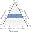 |
Fig. 5 Distribution of the SiO2, MgO, and FeO mole fractions of the training set. |
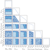 |
Fig. 6 Distribution of the forward model input parameters as generated for the training set. The underlying distributions from which the parameters were generated are listed in Table 3. |
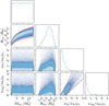 |
Fig. 7 Distribution of the forward model output parameters as generated for the training set. The underlying distributions from which the parameters were generated are listed in Table 3. The solid red lines indicate the limits of the forward model, as described in Sect. 2.3. The light shaded areas in the 2D diagrams indicate the 68% HDR, and the dark shaded areas are the 89%-HDR. |
2.4.2 Data preprocessing
Before any training and prediction was performed, the data were preprocessed. First, we transformed the physical parameters x and observables y into log-space. This ensures that the physical parameters stay strictly positive, while it also reduces magnitude differences between different physical quantities. This is important because vastly different magnitudes between parameters can cause training instabilities, for instance, because a single parameter might dominate the target function (loss) that is minimized during the training procedure. To further address this issue, we also centered both x and y and rescaled them, such that their standard deviations became unity by subtracting and then dividing by the per parameter and observation means and standard deviations, respectively. These linear scaling transformations are easily inverted at prediction time. The scaling transformation parameters were derived from the training set, and the same transformations were applied to new data at prediction time.
2.4.3 Evaluating the training performance
To quantify the success of the cINN training procedure, we proceeded as in Ksoll et al. (2020). We measured its performance on a test data set, a held-out subset of the training data consisting of 20 000 randomly selected synthetic observations. On this test set, we then first confirmed whether the distribution of latent variables had converged to match the target multivariate normal distribution with unit covariance matrix. We settled for this small test set for our final performance evaluation because we found negligible performance differences in comparison to using a larger held-out test set (e.g., 30%), and we wished to provide the exact performance for the best-informed cINN that was later applied to the real observational data.
Afterward, we evaluated the shape of the predicted posterior distributions by computing the median calibration error s, as proposed in Ardizzone et al. (2019a), for each of the target parameters x. Given an uncertainty interval q, the calibration error ecal,q for a collection of N observations is defined as the difference
 (24)
(24)
where qinliers = Ninliers/N denotes the fraction of observations, where the true value  lies within the q-confidence interval of the predicted posterior PDF. Values of ecal,q < 0 signify that the predicted PDFs are too narrow, whereas positive values suggest the opposite, that is, that the PDFs are too broad. The median calibration error s was derived as the median of the absolute calibration errors over the range of confidences from 0 to 1.
Next, we quantified the cΓNNs predictive capability for maximum a posteriori (MAP) point estimates  . To do this, we derived an accuracy for the individual target parameters x over the entire test set as given by the root mean squared error (RMSE) and normalized RMSE (NRMSE). They are defined as
 (25)
(25)
where  is the ground-truth value of the target parameter for the ith observation, and
 (26)
(26)
where  denotes the range of parameter x within the training data. To determine the MAP estimates
  from the predicted samples of the posterior distribution, we performed a kernel density estimation (KDE) to model the PDF and find its maximum. This KDE employed a Gaussian kernel function and was computed on an evenly spaced grid of 1024 points, covering the full range of the given posterior samples. The kernel bandwidth h was derived using Silverman’s rule (Silverman 1986),
 (27)
(27)
where IQR, σ, and n denote the interquartile range, standard deviation, and number of the posterior samples, respectively.
2.4.4 Predicting posteriors for noisy observations
As the method was outlined so far, the cINN did not include the possibility that a given input observation can be uncertain. Instead, the described method assumed perfect observations as an input. However, in many real-world applications, all observed quantities usually have measurement uncertainties. In order to predict the posterior probability distribution of x given a noisy observation using the cINN, we devised the following strategy.
Let the noisy observation be represented by y* and the true observable properties of the target be denoted as y. For this paper, we assumed that the distribution of y* follows a multivariate normal distribution of dimension k with mean μ and covariance Σ, that is,
 (28)
(28)
Given the law of total probability, the posterior probability distribution p(x | y*) can be written as
 (29)
(29)
where y′ is a point in the space of observational parameters, and Φy′|y* is the probability density function of y′ given y*. Because we assumed that y* follows a multivariate normal distribution, Φy′|y* is given by
 (30)
(30)
Next we used that x is conditionally independent of y* given y, that is, ((x ⊥ y*) | y). It follows that p(x | y* ∩ y) = p(x | y) and hence
 (31)
(31)
where p(x | y = y′) can be calculated for a given y′ from Eq. (5).
The posterior probability distribution can now be calculated using simple Monte Carlo integration. Here the Monte Carlo samples of x were generated by first drawing N times a sample y′i from the multivariate normal distribution given in Eq. (28). For each sample y′i, we then calculated the point estimate of p(x|y′i) using the cINN as outlined in Sect. 2.1.1. For each y′i, we therefore sampled another M times from the latent variables z and evaluated for each zi the backward mapping of the cINN, that is, g(zi, c = y′i).
This resulted in N × M samples of x drawn from the posterior probability distribution p(x | y*). By definition, the conditional probability p(x | y) is zero if p(x) = 0 or p(y) = 0. Hence, if the prior distribution of x has a compact support, then p(x | y) is automatically zero for any x outside of the domain of x. While the extent of the domain is in principle learned by the cINN, it is still possible that the cINN maps some zi to an x for which p(x) = 0. During the sampling of z, all such samples should thus be rejected. Additionally, the compact support of p(x) simultaneously limits the possible output values of the forward model and therefore also induces limits on y. We can hence forgo evaluating the cINN for any y′i for which p(y′i) = 0. The kind of limits introduced for y depend on the forward model. We discuss this aspect in more detail in Sect. 2.3.
3 Method validation
In order to validate the sampling scheme outlined in Sect. 2, we used a simple toy model to benchmark the proposed scheme against a common Metropolis-Hastings MCMC sampler. We wished to test here in particular how the sampling performs when i) the posterior distribution of the model parameters has nonzero probability along the boundary of the prior domain, and ii) the observation is close to a region in which the forward model can no longer be applied. This will in particular demonstrate how the method performs when an observation is close to the border of the set of training data.
To mimic situations (i) and (ii), we set up the following toy model. We defined the space of model parameters x = (x1, x2) ∈ ℝ2, as well as the space of observable features y = (y1, y2) ∈ ℝ2. The forward model f(x) is given by the linear model
![Mathematical equation: $f\left( {\left[ {\matrix{ {{x_1}} \cr {{x_2}} \cr } } \right]} \right) = \left[ {\matrix{ 1 & 0 \cr 1 & 2 \cr } } \right]\,\left[ {\matrix{ {{x_1}} \cr {{x_2}} \cr } } \right] = \left[ {\matrix{ {{y_1}} \cr {{y_2}} \cr } } \right].$](/articles/aa/full_html/2023/04/aa43230-22/aa43230-22-eq40.png) (32)
(32)
The prior domain is given by an equilateral triangle in the space of model parameters, defined by its corners,
![Mathematical equation: ${{\bf{c}}_1} = \left[ {\matrix{ 0 \cr 0 \cr } } \right],{{\bf{c}}_2} = \left[ {\matrix{ 1 \cr 0 \cr } } \right],{{\bf{c}}_3} = \left[ {\matrix{ {0.5} \cr {0.5\sqrt 3 } \cr } } \right].$](/articles/aa/full_html/2023/04/aa43230-22/aa43230-22-eq41.png) (33)
(33)
For simplicity, we chose a uniform prior probability distribution within the prior domain. p(x) is therefore written as
 (34)
(34)
where the probability to be within the triangle is the inverse of the area of the triangle. For a noisy observation y* defined as in Eq. (28), that is, as a multivariate normal distribution,
![Mathematical equation: ${{\bf{y}}^ * } \sim {_2}\left( {{\bf{\mu }} = \left[ {\matrix{ {0.4} \cr {1.3} \cr } } \right],\sum = \left[ {\matrix{ {{{0.1}^2}} & 0 \cr 0 & {{{0.1}^2}} \cr } } \right]} \right),$](/articles/aa/full_html/2023/04/aa43230-22/aa43230-22-eq43.png) (35)
(35)
the posterior distribution on x will become heavily truncated by the prior domain. To mimic case (ii), we further added a restriction on the observable parameter y2 and arbitrarily set an upper limit of
 (36)
(36)
The cINN was then trained on a dataset containing 106 samples of x and corresponding f(x) values. This number of training samples is larger than necessary. As the training samples are cheap to generate, we forwent finding an optimal number of training samples. Given y* as in Eq. (35), we then followed the method outlined in Sect. 2.4.4 to sample from the posterior distribution. The resulting distributions from the cINN and the MCMC sampling are shown in Fig. 8, with the summary statistics of the marginalized distributions listed in Table 4. The summary statistics of the marginalized distributions show that the median of each variable does not vary between methods. Moreover, the centered 1σ interval (containing 68.3% of all samples) and the centered 2σ interval (containing 95.4% of all samples) are almost identical (except for a 0.01 deviation of the lower bound of the 1σ interval of y2 and the upper bound of the 2σ interval of x1). To compare the shape of the resulting distributions, we also computed the Hellinger distance h between the marginalized probability distributions of the two methods.
The Hellinger distance h(r, q) between two discrete probability distributions r and q is given by
 (37)
(37)
where b(r, q) is the Bhattacharyya coefficient (see Hellinger 1909),
 (38)
(38)
The Hellinger distance is a proper distance metric. It is zero if the distributions r and q are identical and one if they are disjoint. Here, the Hellinger distance was determined from the histograms of the 1D marginalized distributions generated using the cINN or MCMC method. The optimal number of bins was estimated using the method of Doane (1976).
We report that the Hellinger distance between the distributions for x1 is h = 0.026, whereas for x2, it is h = 0.022. For the observable features, the Hellinger distance has similarly low values of h = 0.023 for y1 and h = 0.046 for y2. For comparison, the Hellinger distance of two normal distributions, where the median of the two distributions differs by 10−1 or 10−2, is h = 0.035 or h = 0.004, respectively. For more details see Table 5.
The 2D marginalized posterior densities in Fig. 8 show that the posterior distribution on the input parameters x1 and x2 is strongly truncated, as expected. Moreover, the upper limit of y2 has a notable effect on the distribution of the input parameters. No major differences between the two methods are visible, however. We conclude that the cINN method can be successfully used for this simple model, even when the observation is close to the boundary of the training data.
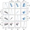 |
Fig. 8 Comparison of the cINN and an MCMC method when applied to the toy model. The data in the lower triangle (black) were predicted by the cINN method, and the data in the upper triangle (blue) were generated with an MCMC sampler. The dashed blue lines indicate the boundaries of the prior domain, outside of which the prior probability is zero. The dashed red line indicates the upper limit on y2 as in Eq. (36). The histograms of the analytical solution are omitted since they overlap with the MCMC data. The light shaded areas in the 2D scatter plots indicate the 68% HDR, and the dark shaded areas are the 89%-HDR. |
4 Results
4.1 Training performance
For the planet characterization task, we trained a cINN to predict the physical parameters Rcore, Rmantle, Rvol (i.e., the radii of the core, mantle, and surface layer, respectively), wcore, wvol,  , xMgO|mantle and xS|core from the observables Mtot, Rtot, xSi/xFe|Planet, and xMg/xFe|Planet, using the database described in Sect. 2.4.1. To fully assess the cINN performance, we would need to generate posterior distributions for a large sample of mock observations spread over the set of training data. To be statistically significant, the number of observations would need to be on the order of ~103–104 cases. Computing the posterior distribution of such a large number of cases using an MCMC method is computationally unfeasible. Instead, we used two complementary methods to assess the performance of the cINN.
4.1.1 Performance on test data
First, we tested the performance of the trained cINN model on synthetic, held-out test data for all the target parameters. As described in Sect. 2.4.3, we computed the RMSE and NRMSE for the MAP point estimates for the test data, as well as the median calibration errors s and median uncertainty at 68% confidence u68 (i.e., the width of the 68% confidence interval) of the posterior distributions. This method allowed us to estimate how well the cINN learned the shape of the posterior distribution for a single-point estimate. The computed values are summarized in Table 6. Figure 9 also provides 2D histograms comparing the MAP estimates against the corresponding ground-truth values. The performance on the synthetic test set was evaluated without error resampling, that is, assuming perfect observations. As the histograms and the RMSEs/NRMSEs demonstrate, the cINN can recover Rcore, Rmantle, Rvol, wcore, wvol, and xMgO|mantle quite well overall with MAP estimates that fall very close or directly on to the ideal one-to-one correlation in comparison to the ground truth. Examining Rcore and Rmantle more closely, we realized some systematic divergences from the one-to-one correlation toward small cores and large mantles, however, indicating that these properties appear to be harder to constrain within these regimes. Likely related to this, we also observed a systematic underestimation of the core mass fraction for very low-mass cores between 0 and 0.1, showing that the cINN also slightly struggles in this range.
For the remaining two properties, xS|core and  , we find that the MAP point estimates cannot match the ground-truth values at all. The results are scattered across the entire parameter ranges with no discernible overdensity at the one-to-one correlation. The median calibration errors s of the underlying predicted posterior distributions show that the cINN finds very well calibrated solutions (i.e., posteriors that are neither too broad nor too narrow) with values below 0.7% for all target parameters, including xS|core and
  . From the median widths of the 68% confidence intervals, which are on the order of ≈0.1 on average, we find, however, that the posterior distributions tend to be rather broad in general (taking the target parameter ranges into account).
For the posterior distributions themselves, the issues with the xS|core and  MAP estimates result from the fact that the cINN consistently predicts almost perfectly uniform distributions across the parameter ranges for these two parameters for all examples in the test set. In this case, performing an MAP estimate simply becomes unfeasible as it merely picks up on minor random fluctuations in these almost uniform distributions rather than identifying distinct peaks in the posteriors. As we show below in our direct comparison of the cINN and an MCMC approach in Sect. 4.2.2, these almost uniform posterior distributions of xS|core and
  are not a flaw of our cINN model, but are also recovered by the MCMC. Because both cINN and MCMC therefore return rather uninformative posterior distributions for xS|core and
  , we have to conclude that these two physical parameters cannot be constrained from the observables Mtot, Rtot, xSi/xFe|Planet, and xMg/xFe|Planet.
Summary statistics (i.e., median centered 1σ interval and centered 2σ interval) of the marginalized posterior distributions of the toy model.
Hellinger distances comparing the marginalized posterior distributions for the toy model.
Overview of cINN test performance for the planet characterization task.
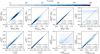 |
Fig. 9 Distribution of N = 20,000 MAP estimates of the trained cINN plotted against the ground truth from the training data set, shown for the model input parameters. |
4.1.2 Recalculation error
Complementary to the analysis of the cINN performance on the test data, we assessed whether the generated posterior samples correctly map back to their corresponding input observations. We performed this by computing the recalculation error ε of the cINN for all four input observables for each posterior sample of 5000 randomly selected synthetic examples from the held-out test set (covering the entire domain of the training data). This means that for each sample x(i) (i.e., predicted set of the eight target parameters) of the 1024 samples generated by the cINN per posterior, we ran the forward model f(·) again and determined the relative difference between the forward model output f(x(i)) and the original network input observation y(i). ε was calculated for each component k of y(i) as
 (39)
(39)
The color-coding in Fig. 10 shows the recalculation error for our four observables as a function of the ground-truth mass and radius. For comparison, we also indicate the position of our real-world test case K2-111 b. With average recalculation errors of  , and
, and  for Mtot, Rtot, xSi/xFe|Planet, and xMg/xFe|Planet, respectively, we find an overall excellent agreement with the input observations. We can conclude that the cINN does indeed return valid posterior distributions on our synthetic test set. Together with the good posterior peak recovery indicated by the low MAP estimate NRMSE for all parameters except xS|core and
  , the cINN has therefore demonstrated a highly satisfactory predictive performance on the synthetic test data.
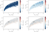 |
Fig. 10 Recalculation error ε of the four observables Mtot, Rtot, xSi/xFe|Planet, and xMg/xFe|Planet as a function of true mass and radius. The black and white encircled cross marks the observed mass and radius of K2-111 b and its corresponding 1σ uncertainties. |
4.2 Comparison between cINN and MCMC for K2-111 b
In order to demonstrate that our cINN provides accurate posterior distributions of planetary parameters, we considered the case of K2-111 b (Mortier et al. 2020), which was observed to be a planet of radius  with amass of
  . Its high mean density of
  implies that the planet is very likely to have only a tiny gas envelope, making it a well-suited example for our purpose. We also assumed that the composition of the photosphere of K2-111 is identical to that of the planet in terms of the elemental ratios of the refractory elements Mg, Fe, and Si. The elemental ratios given in Mortier et al. (2020) are
  for Si/Fe and
  for Mg/Fe. With this observation, we sampled the posterior distribution of the forward model parameters using the cINN method as described in Sect. 2.4.4.
4.2.1 MCMC setup
For this comparison, we also sampled the posterior probability distribution using an MCMC method, as is often employed to infer planetary interiors (see, e.g., Haldemann et al., in prep.; Dorn et al. 2017a). In particular, we used the adaptive Metropolis-Hastings MCMC algorithm (Haario et al. 2001), sampling the posterior distribution of
 (40)
(40)
given the same forward model f(·) as described in Sect. 2.2. We considered the same prior ℙ(x) as we used to construct the training data (see Table 3). The likelihood 𝕃(yobs|x) was calculated using
 (41)
(41)
where μ and σ2 are the mean and variance of yobs and N is the number of dimensions or parameters of yobs.
The MCMC was initialized at a random location in the sample space. We then ran the MCMC for ~5 × 10⁵ steps. The resulting Markov chain had an autocorrelation time τ between 28 and 44 steps for the four output parameters (see Fig. 11). The autocorrelation time was calculated following Hogg & Foreman-Mackey (2018).
To generate independent samples from the Markov chain, we began by discarding the first 2000 steps along the Markov chain due to burn in, and then, accounting for the maximum autocorrelation time, add every 50th step along the chain to the set of independent samples. This resulted in a total of 104 independent samples from the Markov chain, which is sufficient given the shape and number of dimensions of the posterior probability distribution.
Various statistics of the marginalized posterior distribution of the forward model parameters.
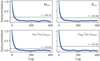 |
Fig. 11 Autocorrelation as a function of lag calculated from the Markov chain of the four output parameters of the forward model. The autocorrelation time τ of each parameter was calculated following Hogg & Foreman-Mackey (2018). The dashed lines indicate the autocorrelation when the lag is equal to the autocorrelation time. |
4.2.2 Comparison of marginalized posterior distributions
In order to compare the performance of the cINN with the MCMC method, we show in Table 7 a summary of the key statistics of the 1D marginalized posterior PDF. For each model parameter, the median as well as the centered 1σ and 2σ intervals (containing 68% and 95% of all samples, respectively) are shown. The median values show that both methods return almost identical results with a maximum difference of ~5.8%. For the boundaries of the centered 1σ and 2σ regions, the differences are larger, notably for the lower boundaries of Rvol, wvol, xS|core, xFeO|mantle, and  . However, the Hellinger distances h between the marginalized posteriors predicted by the two methods are very low (h < 0.05) for all parameters, except for Rvol, wvol, and Rtot (see Table 8). The largest Hellinger distance of 0.103 for Rvol is equivalent to the distance of two standard normal distributions whose median is shifted by 0.25. The fact that Rvol has the largest error here is an odd result at first glance because Rvol appeared to be one of the best-constrained parameters in our test on the synthetic data. There are multiple possible explanations for this result. First, this might simply be an effect of the uncertainty of the observables, which are taken into account here, but not in our previous synthetic test. Second, although the MAP estimates for Rvol are indeed overall quite excellent, there are a few statistical outliers with slightly larger discrepancies as well, so that the result for K2-111 b may just be one such outlier. Last, it is also important to note that the MAP RMSE and the Hellinger distance measure two different properties of the predicted posterior distributions. The former quantifies the point estimation capability, that is, the ability of the cINN to recover the true value as the most likely peak in the posterior distribution. The latter, on the other hand, quantifies a difference in the shape of the posterior with respect to the MCMC ground truth. It might therefore be that the shape of the Rvol posteriors in our synthetic test also tends to deviate slightly more from the ground-truth shape, even though the low MAP NRMSE indicates that they have the correct peak. Unfortunately, due to the prohibitive computational cost of running the MCMC for a statistically large enough sample of the synthetic test data, we were unable to quantify this effect in our previous test.
In Figs. 12 and 13, we show the pairwise marginalized 2D posterior PDF of all parameters. In the diagonal of these figures, we also show the 1D histograms of the marginalized PDF, as well as the prior distribution of the points in the training data. Overall, the shape of the pairwise marginalized 2D posterior PDF is very similar between the two methods. Figure 13 also shows that the cINN method can be used close to the boundary of the training data (red lines). For the 1D histograms, the largest difference is again seen for Rvol and wvol, especially toward dry compositions.
The layer mass fractions and the mantle composition are each a set of compositional variables (hence they sum up to one). Their distribution on the ternary diagram is therefore shown in Fig. 14. For the layer mass fractions, the agreement in the region above 0.1 wvol is very good. Because this is also present in the 1D marginalized distributions, there are fewer samples with low volatile content in the Markov chain than in the set generated using the cINN. For the mantle composition, the posterior distribution of both methods is centered around compositions with 60% MgO and less than 10% FeO. Compared to the MCMC method, the cINN predicts slightly more compositions with larger amounts of SiO2 than MgO, which results in the two kinks in the contours in the ternary diagram.
Hellinger distance metric between the marginalized posterior distributions of the cINN and MCMC method.
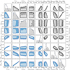 |
Fig. 12 Comparison of the cINN and an MCMC method when applied to K2-111 b. The data in the lower triangle of each panel (blue points) were generated with the cINN method, and the data in the upper triangle (black points) were generated with the MCMC sampler. In the diagonal panels, we also show the marginalized prior probability (gray). The light shaded areas in the 2D diagrams indicate the 68% HDR, and the dark shaded areas are the 89% HDR. |
4.2.3 Recalculation error of trained cINN for K2-111 b
To assess the quality of the inverse mapping from y to x, we calculated the recalculation error ϵ for each sample x(i) generated with the cINN according to Eq. (39). In Fig. 15, we show the distribution of the recalculation errors of all data variables together with wvol, given the set of x(i) generated for the case of K2-111 b. The cINN learned the mapping of the total mass best, and the median recalculation error of the other variables is between 1.3% and 2.5%. Figure 15 also indicates that the recalculation errors increase toward low values of wvol, especially below 0.1. This indicates that the quality of the cINN mapping in this region is not yet optimal. This likely explains the observed differences in the posterior distribution of wvol and Rvol between the MCMC and the cΓNN method.
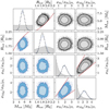 |
Fig. 13 Comparison of cINN and MCMC posteriors when applied to K2-111 b. The colors and shadings are the same as in Fig. 12. The solid red line indicates the limits of the forward model, as discussed in Sect. 2.3. |
5 Discussion
5.1 Comparison to the initial characterization of K2-111 b
The exoplanet K2-111 b was also characterized in Mortier et al. (2020). In their work, two different internal structure models were used for characterization, one considering four layers, that is, an iron core, a silicate mantle, a water layer, and an H/He envelope. The other model only considered two layers, that is, an iron core with a surrounding mantle. In the first model, the inferred bulk composition of K2-111 b was  , and
, and  . The inferred small amount of H/He by Mortier et al. (2020) is one reason we chose this exoplanet for our work because we trained the cINN only on planetary structures without H/He layers so far.
When we compare this to the results obtained using the cINN, which are given in Table 7, we see that the inferred core mass fraction is almost the same, while the mantle mass fraction is slightly smaller and the water mass fraction is slightly larger than in Mortier et al. (2020). They also inferred a mantle composition of  and
and  , together with a core composition of
  . This also agrees well with the prediction results of the cINN. We note, however, that the good agreement in xS|core and
  may only be by chance here, as both the cINN and MCMC regard these two parameters as largely unidentifiable from the available observations (see Sect. 4.1). At the same time, the inference method used in Mortier et al. (2020) can merely constrain xS|Core and
  beyond the constraints given by the used structure model.
The reason for the small difference in the mantle mass fraction and water mass fraction is likely that they used a four-layer model, including a H/He layer. Although K2-111 b has a very small H/He content in mass (~10−8 ME as found in Mortier et al. 2020), this small H/He layer can still contribute to radius by ~0.1 Re, given the high equilibrium temperature of the planet (Teq = 1309 K). Thus, our results are expected to differ slightly from their study. Taking the difference in model setup into account, we conclude that our results agree well with the characterization performed by Mortier et al. (2020).
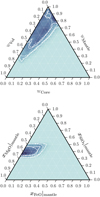 |
Fig. 14 Ternary diagrams of the cINN prediction. Top panel: kernel density estimate of the layer mass fractions as determined with the cINN. Bottom panel: kernel density estimate of the mantle composition. The kernel density in both panels was estimated using a Gaussian kernel with a standard deviation of 0.2. The white lines indicate the contours of the 68% HDR and 95% HDR. For comparison, the HDR from the posterior calculated with the MCMC is also shown (dashed lines). |
5.2 Comparison of the computational cost
One main motivation for using cINNs to infer planetary compositions is to reduce the time needed to perform a single inference. We provide here an overview over the encountered computational cost when using the two methods shown in this work, that is, an adaptive Metropolis Hastings MCMC method and the cINN method.
The MCMC method is calculated sequentially, that is, for each step of the Markov chain, a forward model is run until a sufficient number of steps are generated. Hence, its computational cost scales linearly with the number of steps of the generated Markov chain. For the forward model we used, it was proven sufficient to generate on the order of 5 × 10⁵ forward models. On a single core of an Intel Xeon Gold 6132 processor running at 2.6 GHz, one forward model takes 1.5 s to compute on average. Therefore, computing one planetary structure inference takes approximately 8.7 days in total on a single core.
Instead of computing a single Markov chain, it is also possible to initialize multiple chains in parallel or use an ensemble method such as in emcee (Foreman-Mackey et al. 2013). This parallelized approach allows leveraging the availability of multicore CPU architectures. For an efficient tuning of the proposal distribution, a minimum length of the Markov chain on the order of ~104 samples is required, however. Using 28 cores of an Intel Xeon Gold 6132 CPU, we had to compute 104 steps for each of the 28 Markov chains to account for burn-in and tuning of the proposal distribution. This results in a total of 7.8 × 10⁵ forward models to be calculated by 28 parallel MCMC chains, which takes approximately 12 h. While the time for a single inference is only a fraction compared to a sequential MCMC run, the total computational cost is equivalent to 13.5 days of single threaded run time. The reason are the larger number of samples, which cannot be used for inference due to burn-in and tuning of the proposal distribution.
The total computational cost of the cINN method in contrary is split into three parts. The computation time needed to generate the training data, the time needed to train the cINN including the search for the hyperparameters for optimal training (i.e., determining learning rate, network architecture, etc.), and the time needed to sample the posterior using the cINN. For this project, the training data were generated calculating 5.9 × 10⁶ forward models. With an average run time of 1.5 s, this would take 102 days to run on a single core, whereas using a compute node with 28 cores, the data set can be generated within 3.7 days. With the training data at hand, training the cfNN itself takes between 2 and 3 h on a single GPU. The training and inference were performed on a compute node at the Interdisziplinäres Zentrum für Wissenschaftliches Rechnen (IWR) in Heidelberg, which consists of 2 × 14-Core Intel Xeon Gold 6132 at 2.6 GHz and 10× Nvidia Titan Xp at 1.6 GHz, but only one GPU was used. Then a hyperparameter search is necessary to find the parameters for optimal training (i.e., learning rate, number of the neural network layers, network layer widths, etc.). For this study, we performed 23 trials to find the optimal parameters, thus repeating the training of the cINN 23 times. A single inference of the composition of an exoplanet using the trained cINN on the same GPU as mentioned above can be performed in 5 min. Performing all preparatory steps, that is, generating the training data, training, and hyperparameter search, takes approximately 105 days of sequential computing time. Leveraging multithreaded CPUs can reduce the runtime of all preparatory steps to 6 days.
When comparing the computational cost of the two methods, it is clear that for a single inference, the MCMC method is far cheaper given the large number of training data needed to train the cINN. When multiple inferences using the same forward model are to be performed, however, then generating the training data will contribute less to the total computational cost the more inferences are performed. Taking into account that the hyperparameter search in both does cases not need to be repeated (except when the MCMC method is used for very different data), then the cINN already becomes the more efficient method if the same forward model is used for more than ten planetary structure inferences. In Table 9 we show a summary of the computational cost of the two methods.
So far, we used a forward model without an additional atmosphere layer. Including an atmosphere in the forward model would add another two to three more input parameters and also make the forward model computationally more expensive. From experience with running structure inference models that include atmosphere layers, a number of 5 × 10⁵–106 samples would be necessary to be generated for the Markov chain. We did not yet create a database of forward models including an atmosphere, hence we cannot conclude how this change would affect the computational cost. The time needed for inference should remain on the order of minutes for the cINN approach, however.
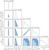 |
Fig. 15 Recalculation errors of the model output variables for the set of samples generated with the cINN for the case of K2-111 b. |
Overview over the computational cost for the two inference methods.
6 Conclusions
We discussed how INNs, in particular, the cINN, can be used to characterize the interior structure of exoplanets. So far, mainly MCMC methods were used to do this.
Compared to the cINN version initially proposed by Ardizzone et al. (2019b) for point estimates, we showed how the method can be adapted for noisy data. We validated this approach using a toy model, for which we compared the cINN performance against a regular Metropolis Hastings MCMC.
Then we applied the method to the exoplanet K2-111 b, inferring its composition. To do this, we trained a cINN on a simplified internal structure model for exoplanets and showed that in this case, cINNs also offer a computationally efficient alternative to the MCMC sampler that is commonly used for Bayesian inference.
In the benchmark of K2-111 b, only minor differences can be seen between the MCMC methods and the cINN method. The largest differences appeared in the marginalized posterior distribution of Rvol and wvol. Computing the recalculation error of the benchmark case showed that the largest errors in total radius appeared for low values of wvol. This agrees with the observed differences in the marginalized posterior distributions of wvol and Rvol. Hence, it is likely that the difference between the two methods will become smaller if the training of the cINN can be further improved. Nevertheless, the two methods return very similar posterior distributions of the model parameters.
A key benefit of using cINNs over an MCMC method is that most of the computational cost of the method occurs during the generation of the training data and training, but not during the inference. This allows reducing the computational time spent for inference by almost four orders of magnitude compared to a regular MCMC method. In order to have an overall benefit in computational cost against the MCMC method used in this work, the cINN needs to be used to infer more than approximately ten planetary structures. While other authors successfully used neural networks to predict the output of their forward models (e.g., Alibert & Venturini 2019; Baumeister et al. 2020), this work showed that it is also possible to train a neural network that encapsulates the full inverse problem.
Acknowledgements
We thank the referee Philipp Baumeister for the insightful comments which helped to improve the manuscript. J.H. and Y.A. acknowledge the support from the Swiss National Science Foundation under grant 200020_172746. V.K. and R.S.K. acknowledge financial support from the European Research Council via the ERC Synergy Grant “ECOGAL” (project ID 855130), from the Deutsche Forschungsgemeinschaft (DFG) via the Collaborative Research Center “The Milky Way System” (SFB 881 – funding ID 138713538 – subprojects A1, B1, B2 and B8), from the Heidelberg Cluster of Excellence (EXC 2181 – 390900948) “STRUCTURES”, funded by the German Excellence Strategy, and from the German Ministry for Economic Affairs and Climate Action in project “MAINN” (funding ID 50OO2206). They also thank for computing resources provided by the Ministry of Science, Research and the Arts of the State of Baden-Württemberg through bwHPC and DFG through grant INST 35/1134-1 FUGG and for data storage at SDS@hd through grant INST 35/1314-1 FUGG. For this publication, the following software packages have been used: Python-matplotlib by Hunter (2007), Python-seaborn by Waskom et al. (2021), Python-corner by Foreman-Mackey (2016) Python-ternary by Harper et al. (2019), Python-numpy, Python-pandas. The cINN implementation is based on the FrEIA framework available at https://github.com/VLL-HD/FrEIA.
References
- Adibekyan, V., Dorn, C., Sousa, S.G., et al. 2021, Science, 374, 330 [NASA ADS] [CrossRef] [Google Scholar]
- Agol, E., Dorn, C., Grimm, S. L., et al. 2021, Planetary Science Journal, 2, 1 [NASA ADS] [CrossRef] [Google Scholar]
- Alibert, Y., & Venturini, J. 2019, A&A, 626, A21 [NASA ADS] [CrossRef] [EDP Sciences] [Google Scholar]
- Ardizzone, L., Kruse, J., Rother, C., & Köthe, U. 2019a, in International Conference on Learning Representations [Google Scholar]
- Ardizzone, L., Lüth, C., Kruse, J., Rother, C., & Köthe, U. 2019b, ArXiv [arXiv:1907.02392] [Google Scholar]
- Atkins, S., Valentine, A. P., Tackley, P. J., & Trampert, J. 2016, Phys. Earth Planet. Interiors, 257, 171 [CrossRef] [Google Scholar]
- Baumeister, P., Padovan, S., Tosi, N., et al. 2020, ApJ, 889, 42 [Google Scholar]
- Benz, W., Ehrenreich, D., & Isaak, K. 2017, in Handbook of Exoplanets, eds. H. J. Deeg, & J. A. Belmonte (Cham: Springer International Publishing), 1 [Google Scholar]
- Benz, W., Broeg, C., Fortier, A., et al. 2021, Exp. Astron., 51, 109 [Google Scholar]
- Bishop, C. M. 1994, Mixture Density Networks (Birmingham: Aston University) [Google Scholar]
- Brown, J. M. 2018, Fluid Phase Equilibria, 463, 18 [CrossRef] [Google Scholar]
- de Wit, R. W. L., Valentine, A. P., & Trampert, J. 2013, Geophys. J. Int., 195, 408 [NASA ADS] [CrossRef] [Google Scholar]
- Dinh, L., Sohl-Dickstein, J., & Bengio, S. 2016, ArXiv e-prints [arXiv:1605.08803] [Google Scholar]
- Doane, D. P. 1976, Am. Statist., 30, 181 [Google Scholar]
- Dorn, C., Khan, A., Heng, K., et al. 2015, A&A, 577, A83 [NASA ADS] [CrossRef] [EDP Sciences] [Google Scholar]
- Dorn, C., Hinkel, N. R., & Venturini, J. 2017a, A&A, 597, A38 [NASA ADS] [CrossRef] [EDP Sciences] [Google Scholar]
- Dorn, C., Venturini, J., Khan, A., et al. 2017b, A&A, 597, A37 [NASA ADS] [CrossRef] [EDP Sciences] [Google Scholar]
- Fei, Y., Murphy, C., Shibazaki, Y., Shahar, A., & Huang, H. 2016, Geophys. Res. Lett., 43, 6837 [NASA ADS] [CrossRef] [Google Scholar]
- Feistel, R., & Wagner, W. 2006, J. Phys. Chem. Ref. Data, 35, 1021 [NASA ADS] [CrossRef] [Google Scholar]
- Foreman-Mackey, D. 2016, J. Open Source Softw., 1, 24 [Google Scholar]
- Foreman-Mackey, D., Hogg, D. W., Lang, D., & Goodman, J. 2013, PASP, 125, 306 [Google Scholar]
- French, M., & Redmer, R. 2015, Phys. Rev. B, 91, 014308 [CrossRef] [Google Scholar]
- Gordon, S., & McBride, B. J. 1994, Computer Program for Calculation of Complex Chemical Equilibrium Compositions and Applications. Part 1: Analysis, Tech. rep., NASA Lewis Research Center [Google Scholar]
- Haario, H., Saksman, E., & Tamminen, J. 2001, Bernoulli, 7, 223 [CrossRef] [Google Scholar]
- Hakim, K., Rivoldini, A., Van Hoolst, T., et al. 2018, Icarus, 313, 61 [Google Scholar]
- Haldemann, J., Alibert, Y., Mordasini, C., & Benz, W. 2020, A&A, 643, A105 [NASA ADS] [CrossRef] [EDP Sciences] [Google Scholar]
- Harper, M., Weinstein, B., Simon, C., et al. 2019, https://doi.org/10.5281/zenodo.2628066 [Google Scholar]
- Hastings, W. K. 1970, Biometrika, 57, 97 [Google Scholar]
- Hellinger, E. 1909, J. Reine Angew. Math., 1909, 210 [CrossRef] [Google Scholar]
- Hoeijmakers, H. J., Ehrenreich, D., Kitzmann, D., et al. 2019, A&A, 627, A165 [NASA ADS] [CrossRef] [EDP Sciences] [Google Scholar]
- Hogg, D. W., & Foreman-Mackey, D. 2018, ApJS, 236, 11 [NASA ADS] [CrossRef] [Google Scholar]
- Hunter, J. D. 2007, Comput. Sci. Eng., 9, 90 [NASA ADS] [CrossRef] [Google Scholar]
- Journaux, B., Brown, J. M., Pakhomova, A., et al. 2020, J. Geophys. Res.: Planets, 125, e2019JE006176 [CrossRef] [Google Scholar]
- Kang, D. E., Pellegrini, E. W., Ardizzone, L., et al. 2022, MNRAS, 512, 617 [CrossRef] [Google Scholar]
- Kingma, D. P., & Dhariwal, P. 2018, ArXiv e-prints [arXiv:1807.03039] [Google Scholar]
- Kippenhahn, R., Weigert, A., & Weiss, A. 2012, Stellar Structure and Evolution, 2nd edn., Astronomy and Astrophysics Library (Berlin Heidelberg: Springer-Verlag) [CrossRef] [Google Scholar]
- Ksoll, V. F., Ardizzone, L., Klessen, R., et al. 2020, MNRAS, 499, 5447 [NASA ADS] [CrossRef] [Google Scholar]
- Lin, Q., Fouchez, D., Pasquet, J., et al. 2022, A&A, 662, A36 [NASA ADS] [CrossRef] [EDP Sciences] [Google Scholar]
- Madhusudhan, N. 2019, ARA&A, 57, 617 [NASA ADS] [CrossRef] [Google Scholar]
- Mazevet, S., Licari, A., Chabrier, G., & Potekhin, A. Y. 2019, A&A, 621, A128 [NASA ADS] [CrossRef] [EDP Sciences] [Google Scholar]
- McBride, B. J., & Gordon, S. 1996, Computer Program for Calculation of Complex Chemical Equilibrium Compositions and Applications II. Users Manual and Program Description, Tech. rep., NASA Lewis Research Center [Google Scholar]
- Metropolis, N., Rosenbluth, A. W., Rosenbluth, M. N., Teller, A. H., & Teller, E. 1953, J. Chem. Phys., 21, 1087 [Google Scholar]
- Mortier, A., Zapatero Osorio, M. R., Malavolta, L., et al. 2020, MNRAS, 499, 5004 [Google Scholar]
- Mosegaard, K., & Tarantola, A. 1995, J. Geophys. Res.: Solid Earth, 100, 12431 [NASA ADS] [CrossRef] [Google Scholar]
- Plotnykov, M., & Valencia, D. 2020, MNRAS, 499, 932 [CrossRef] [Google Scholar]
- Press, W. H., Teukolsky, S. A., Vetterling, W. T., & Flannery, B. P. 1996, Numerical Recipes in Fortran 90: Vol. 2, Volume 2 of Fortran Numerical Recipes: The Art of Parallel Scientific Computing (Cambridge University Press) [Google Scholar]
- Rauer, H., & Heras, A. M. 2018, in Handbook of Exoplanets, eds. H. J. Deeg, & J. A. Belmonte (Cham: Springer International Publishing), 1309 [CrossRef] [Google Scholar]
- Rogers, L. A., & Seager, S. 2010, ApJ, 712, 974 [Google Scholar]
- Schulze, J. G., Wang, J., Johnson, J. A., et al. 2021, Planet. Sci. J., 2, 113 [NASA ADS] [CrossRef] [Google Scholar]
- Silverman, B. W. 1986, Density estimation for Statistics and Data Analysis (Chapman and Hall) [Google Scholar]
- Sotin, C., Grasset, O., & Mocquet, A. 2007, Icarus, 191, 337 [Google Scholar]
- Thiabaud, A., Marboeuf, U., Alibert, Y., Leya, I., & Mezger, K. 2015, A&A, 580, A30 [NASA ADS] [CrossRef] [EDP Sciences] [Google Scholar]
- Trotta, R. 2008, Contemp. Phys., 49, 71 [Google Scholar]
- Wagner, W., & Pruß, A. 2002, YJARS58457 J. Phys. Chem. Ref. Data, 31, 387 [NASA ADS] [CrossRef] [Google Scholar]
- Waskom, M., Gelbart, M., Botvinnik, O., et al. 2021, mwaskom/seaborn/10.5281/zenodo.592845 [Google Scholar]
All Tables
Summary statistics (i.e., median centered 1σ interval and centered 2σ interval) of the marginalized posterior distributions of the toy model.
Hellinger distances comparing the marginalized posterior distributions for the toy model.
Various statistics of the marginalized posterior distribution of the forward model parameters.
Hellinger distance metric between the marginalized posterior distributions of the cINN and MCMC method.
All Figures
|
Fig. 1 Schematic overview of a Metropolis Hastings MCMC algorithm. The MCMC algorithm generates samples x(0) … x(n) ~ π, where the distribution π is proportional to the posterior probability p(x|y). |
| In the text | |
|
Fig. 2 Schematic overview of the cINN. During training, the cINN learns to encode all information about the physical parameters x in the latent variables z (while enforcing that they follow a Gaussian distribution) that is not contained in the observations y. At prediction time, conditioned on the new observation y, the cINN then transforms the known prior distribution p(z) to x-space to retrieve the posterior distribution p(x|y). |
| In the text | |
|
Fig. 3 Schematic overview over the cINN architecture. |
| In the text | |
|
Fig. 4 Schematic representation of the layered planetary structure. Three main layers are present: the core, silicate mantle, and volatile layer. Depending on the size of the layers, an upper mantle can be present if the volatile layer above is not too massive. Conversely, if the volatile layer is massive enough, high-pressure ices might form on the bottom of the layer. |
| In the text | |
|
Fig. 5 Distribution of the SiO2, MgO, and FeO mole fractions of the training set. |
| In the text | |
|
Fig. 6 Distribution of the forward model input parameters as generated for the training set. The underlying distributions from which the parameters were generated are listed in Table 3. |
| In the text | |
|
Fig. 7 Distribution of the forward model output parameters as generated for the training set. The underlying distributions from which the parameters were generated are listed in Table 3. The solid red lines indicate the limits of the forward model, as described in Sect. 2.3. The light shaded areas in the 2D diagrams indicate the 68% HDR, and the dark shaded areas are the 89%-HDR. |
| In the text | |
|
Fig. 8 Comparison of the cINN and an MCMC method when applied to the toy model. The data in the lower triangle (black) were predicted by the cINN method, and the data in the upper triangle (blue) were generated with an MCMC sampler. The dashed blue lines indicate the boundaries of the prior domain, outside of which the prior probability is zero. The dashed red line indicates the upper limit on y2 as in Eq. (36). The histograms of the analytical solution are omitted since they overlap with the MCMC data. The light shaded areas in the 2D scatter plots indicate the 68% HDR, and the dark shaded areas are the 89%-HDR. |
| In the text | |
|
Fig. 9 Distribution of N = 20,000 MAP estimates of the trained cINN plotted against the ground truth from the training data set, shown for the model input parameters. |
| In the text | |
|
Fig. 10 Recalculation error ε of the four observables Mtot, Rtot, xSi/xFe|Planet, and xMg/xFe|Planet as a function of true mass and radius. The black and white encircled cross marks the observed mass and radius of K2-111 b and its corresponding 1σ uncertainties. |
| In the text | |
|
Fig. 11 Autocorrelation as a function of lag calculated from the Markov chain of the four output parameters of the forward model. The autocorrelation time τ of each parameter was calculated following Hogg & Foreman-Mackey (2018). The dashed lines indicate the autocorrelation when the lag is equal to the autocorrelation time. |
| In the text | |
|
Fig. 12 Comparison of the cINN and an MCMC method when applied to K2-111 b. The data in the lower triangle of each panel (blue points) were generated with the cINN method, and the data in the upper triangle (black points) were generated with the MCMC sampler. In the diagonal panels, we also show the marginalized prior probability (gray). The light shaded areas in the 2D diagrams indicate the 68% HDR, and the dark shaded areas are the 89% HDR. |
| In the text | |
|
Fig. 13 Comparison of cINN and MCMC posteriors when applied to K2-111 b. The colors and shadings are the same as in Fig. 12. The solid red line indicates the limits of the forward model, as discussed in Sect. 2.3. |
| In the text | |
|
Fig. 14 Ternary diagrams of the cINN prediction. Top panel: kernel density estimate of the layer mass fractions as determined with the cINN. Bottom panel: kernel density estimate of the mantle composition. The kernel density in both panels was estimated using a Gaussian kernel with a standard deviation of 0.2. The white lines indicate the contours of the 68% HDR and 95% HDR. For comparison, the HDR from the posterior calculated with the MCMC is also shown (dashed lines). |
| In the text | |
|
Fig. 15 Recalculation errors of the model output variables for the set of samples generated with the cINN for the case of K2-111 b. |
| In the text | |
Current usage metrics show cumulative count of Article Views (full-text article views including HTML views, PDF and ePub downloads, according to the available data) and Abstracts Views on Vision4Press platform.
Data correspond to usage on the plateform after 2015. The current usage metrics is available 48-96 hours after online publication and is updated daily on week days.
Initial download of the metrics may take a while.