| Issue |
A&A
Volume 676, August 2023
|
|
|---|---|---|
| Article Number | A106 | |
| Number of page(s) | 14 | |
| Section | Numerical methods and codes | |
| DOI | https://doi.org/10.1051/0004-6361/202346216 | |
| Published online | 17 August 2023 | |
ExoMDN: Rapid characterization of exoplanet interior structures with mixture density networks★,★★
1
Institute of Planetary Research, German Aerospace Center (DLR),
Rutherfordstraße 2,
12489
Berlin,
Germany
e-mail: This email address is being protected from spambots. You need JavaScript enabled to view it.
2
Department of Astronomy and Astrophysics, Technische Universität Berlin,
Hardenbergstraße 36,
10623
Berlin,
Germany
Received:
22
February
2023
Accepted:
14
June
2023
Abstract
Aims. Characterizing the interior structure of exoplanets is essential for understanding their diversity, formation, and evolution. As the interior of exoplanets is inaccessible to observations, an inverse problem must be solved, where numerical structure models need to conform to observable parameters such as mass and radius. This is a highly degenerate problem whose solution often relies on computationally expensive and time-consuming inference methods such as Markov chain Monte Carlo.
Methods. We present ExoMDN, a machine-learning model for the interior characterization of exoplanets based on mixture density networks (MDN). The model is trained on a large dataset of more than 5.6 million synthetic planets below 25 Earth masses consisting of an iron core, a silicate mantle, a water and high-pressure ice layer, and a H/He atmosphere. We employ log-ratio transformations to convert the interior structure data into a form that the MDN can easily handle.
Results. Given mass, radius, and equilibrium temperature, we show that ExoMDN can deliver a full posterior distribution of mass fractions and thicknesses of each planetary layer in under a second on a standard Intel i5 CPU. Observational uncertainties can be easily accounted for through repeated predictions from within the uncertainties. We used ExoMDN to characterize the interiors of 22 confirmed exoplanets with mass and radius uncertainties below 10 and 5%, respectively, including the well studied GJ 1214 b, GJ 486 b, and the TRAPPIST-1 planets. We discuss the inclusion of the fluid Love number k2 as an additional (potential) observable, showing how it can significantly reduce the degeneracy of interior structures. Utilizing the fast predictions of ExoMDN, we show that measuring k2 with an accuracy of 10% can constrain the thickness of core and mantle of an Earth analog to ≈13% of the true values.
Key words: planets and satellites: interiors / planets and satellites: composition / methods: numerical / methods: statistical
Full Table A.1 is only available at the CDS via anonymous ftp to cdsarc.cds.unistra.fr (130.79.128.5) or via https://cdsarc.cds.unistra.fr/viz-bin/cat/J/A+A/676/A106
ExoMDN is freely accessible through the GitHub repository https://github.com/philippbaumeister/ExoMDN
© The Authors 2023
 Open Access article, published by EDP Sciences, under the terms of the Creative Commons Attribution License (https://creativecommons.org/licenses/by/4.0), which permits unrestricted use, distribution, and reproduction in any medium, provided the original work is properly cited.
This article is published in open access under the Subscribe to Open model. This email address is being protected from spambots. You need JavaScript enabled to view it. to support open access publication.
1 Introduction
In the past decade, the number of discovered exoplanets has been growing rapidly, with more than 5000 planets confirmed to date. Characterizing the interior structures of these planets, that is, the size and mass of their main compositional reservoirs, is critical to understanding the processes that govern their formation, evolution, and potential to support life (Spiegel et al. 2014; Van Hoolst et al. 2019). Numerical models are commonly used to compute interior structures that fit to observed mass and radius of the planet (e.g., Sotin et al. 2007; Valencia et al. 2007; Fortney et al. 2007; Wagner et al. 2011; Zeng & Sasselov 2013; Unterborn & Panero 2019; Baumeister et al. 2020; Huang et al. 2022). However, unlike planets in the Solar System for which a wealth of observational data is available ranging from geodetic observations to in situ seismic measurements, for exoplanets, mass and radius are often the only parameters that can be determined. As a result, the interior structure is highly degenerate, with many qualitatively different interior compositions that can match the observations equally well (Rogers & Seager 2010; Dorn et al. 2015, 2017b; Brugger et al. 2017). Probabilistic inference methods, such as Markov chain Monte Carlo (MCMC) sampling, are regularly utilized to obtain a comprehensive picture of possible planetary interiors, while also taking into account observational uncertainties (Rogers & Seager 2010; Dorn et al. 2015, 2017b; Dorn & Heng 2018; Acuña et al. 2021). Given prior estimations of interior parameters, probabilistic inference methods allow for the determination of posterior probabilities that best fit the observations. However, in general, MCMC methods are computationally intensive and time-consuming, requiring calculations of hundreds of thousands of interior structure models. The interior inference of a single exoplanet can therefore take from hours to days. Furthermore, a dedicated framework combining both a forward interior structure model and an MCMC scheme is necessary, which can limit the large-scale applicability of these techniques due to the need for specialized expertise in planetary interior modeling. To fully exploit the ever-increasing number of exoplanet detections, a fast alternative to MCMC inference is needed.
Here, we present ExoMDN, a standalone machine-learning-based model that is capable of providing a full inference of the interior structure of low-mass exoplanets in under a second without the need for a dedicated interior model. We have made both the trained models and the training routines available in a GitHub repository1. The purpose of ExoMDN is to provide a rapid first general characterization of an exoplanet interior, which can then be investigated further with more detailed, specialized models.
2 Machine Learning for interior characterization
In recent years, machine-learning based methods have become increasingly relevant in planetary science because of their ability to facilitate and speed up otherwise very time-consuming calculations. Deep neural networks in particular have been applied to the detection of transits (Chaushev et al. 2019; Malik et al. 2021; Valizadegan et al. 2022), for atmospheric retrievals (Márquez-Neila et al. 2018; Zingales & Waldmann 2018; Himes et al. 2022), in geodynamic simulations (Atkins et al. 2016; Agarwal et al. 2021a,b), in planet formation models (Alibert & Venturini 2019; Cambioni et al. 2019; Emsenhuber et al. 2020; Auddy et al. 2022), as well as for characterizing exoplanet interiors (Baumeister et al. 2020; Zhao & Ni 2021; Haldemann et al. 2023).
In an earlier work (Baumeister et al. 2020), we presented a proof-of-concept method to characterize exoplanet interiors using mixture density networks (MDNs; Bishop 1994), which can predict the full probability distribution of parameters by approximating these with a linear combination of Gaussian kernels. We trained an MDN to infer the range of plausible thicknesses of compositional layers in a planet based on mass and radius inputs. However, this was not a full characterization of the interior, as our network could only predict the marginals of the posterior distribution. While this gives an accurate estimation of the range of admissible parameter values, it does not allow us to pinpoint specific interior structures that fit observed mass and radius nor determining correlations between the various layers. For this purpose, the prediction of the full, multidimensional posterior distribution is required.
ExoMDN builds upon our previous work and is capable of providing a full inference of the entire posterior distribution of interior structures for a planet in a fraction of a second (e.g., on a standard Intel i5 CPU). In addition, we include the equilibrium temperature of the planet as an input parameter to the network in addition to mass and radius, by improving on the atmosphere and water layers in the underlying forward model used to generate the training data. In particular, we used the full water phase diagram compiled by Haldemann et al. (2020) in place of the previous simple isothermal, high-pressure ice layer and we modeled an isothermal atmosphere instead of the previous zero-temperature approach. The use of the equilibrium temperature thus implicitly includes the orbital distance as an observable parameter. We further improved the robustness of the underlying forward model at high pressures by adopting updated high-pressure equations of state (EoS) for the silicate mantle and iron core. A comparison of the old and new forward models can be found in Fig. B.5.
We used our interior model to first generate a dataset of ≈5.6 million synthetic planets spanning the desired parameter space of interior structures, planet masses, and equilibrium temperatures. We then trained a mixture density network to predict the parameters of a mixture of multivariate normal distributions, with the aim of approximating the posterior distribution for a given set of input parameters, namely, mass, radius, and equilibrium temperature. In order for the MDN to handle multidimensional predictions, we applied log-ratio transformations on the training data to convert the interior structures into new coordinates that the MDN can easily handle. We present two trained models: one trained on planetary mass, radius, and equilibrium temperature and the second including the fluid Love number k2 as an additional input. Fluid Love numbers describe the shape of a rotating planet in hydrostatic equilibrium. The second-degree Love number k2 is particularly interesting for exoplanet interior characterization, as it depends solely on the interior density distribution (Kellermann et al. 2018; Padovan et al. 2018; Baumeister et al. 2020). In a body with k2 = 0, the entire mass is concentrated in the center, while k2 = 1.5 corresponds to a fully homogeneous body. For a number of exoplanets, k2 is potentially measurable through either second-order effects on the shape of the transit light curve (Hellard et al. 2019; Akinsanmi et al. 2019), or through the apsidal precession of the orbit (Csizmadia et al. 2019).
3 Methods
3.1 Interior model
We compute planetary interior structures with our code TATOOINE (Baumeister et al. 2020; MacKenzie et al. 2023). Each planet consists of compositionally distinct layers. The model takes as input the planet mass, Mp, the mass fractions of each layer, wi, and the equilibrium temperature, Teq (defined at the top of the atmosphere). From the top of the planet toward the center, the model calculates radial profiles of mass, m, pressure, P, and density, ρ, by solving the equations for mass conservation (1a), hydrostatic equilibrium (1b), as well as the equation of state (EoS, 1c) relating pressure, density, temperature, T, and composition, c:
 (1a)
(1a)
 (1b)
(1b)
 (1c)
(1c)
where G is the gravitational constant. The planet radius, Rp, is iteratively adjusted until the mass at the planet center approaches zero. This yields a final planet radius and the radius fractions of each layer di. We fix the pressure at the top of the atmosphere to 10 mbar. We focus here on planets below 25 M⊕. We consider four distinct layers: an iron core, a silicate mantle, a water layer, and an H/He atmosphere.
3.1.1 Iron core
We assumed that the core consists of pure, solid, hcp-iron. We used the temperature-dependent, high-pressure EoS by Bouchet et al. (2013) for pressures below 234.4 GPa. At higher pressures, we switch to the high-pressure EoS from Hakim et al. (2018), valid up to 10 TPa.
The presence of lighter elements in the core such as sulfur or hydrogen can significantly reduce the density of the core, which in turn can have large effects on the core size and consequently on the planet radius (Hakim et al. 2018). The amount of lighter elements in an exoplanet’s core is hard to constrain, as it not only depends on the initial abundances in the protoplanetary disk, but also on the processes of core formation and magma ocean cooling (Hirose et al. 2021). For a proper treatment of the interior inference, the amount of light elements should be taken as a free parameter, which will increase the degeneracy of interior structures even more. For simplicity and to better illustrate our method, here we neglect the presence of lighter elements in the core, following an approach commonly used in the exo-planet community (e.g., Seager et al. 2007; Wagner et al. 2011). Nevertheless, we note that the uncertainty in the light elements budget of the core can be easily incorporated into our method by sampling from a range of core compositions upon creating the training dataset (Sect. 3.4).
3.1.2 Silicate mantle
The silicate layer consists of an upper mantle composed of olivine (Mg, Fe)2SiO4 and pyroxene (Mg, Fe)2Si2O6, a lower mantle composed of magnesiowüstite (Mg, Fe)O and bridgmanite (Mg, Fe)SiO3, and a high-pressure phase of magnesiowüstite and post-perovskite. The transition from upper to lower mantle is assumed to occur at a fixed pressure of 23 GPa, and the transition to post-perovskite at a pressure of:
 (2)
(2)
following Tateno et al. (2009), where T is the adiabatic temperature in the mantle. We model the upper and lower mantle with a modified Tait EoS from Holland & Powell (2011) and the post-perovskite phase with the generalized Rydberg EoS described in Wagner et al. (2011).
Similar to the composition of the core, the mantle composition could be varied, for example, using stellar abundances as proxies of planet composition (e.g., Dorn et al. 2017a; Hinkel & Unterborn 2018). However, since the relation between star and planet composition is not straightforward (Plotnykov & Valencia 2020), for simplicity, we assume the silicate mantle to have an Earth-like composition with a molar Mg/Si ratio of 1.131 and a magnesium number (Mg#) of 0.9 (Sotin et al. 2007). The Mg/Si ratio determines the mixing ratio of the respective mantle minerals, with the Mg# determining the ratio of the respective Mg and Fe end members.
3.1.3 Water layer
For the water layer, we used the tabulated AQUA EoS from Haldemann et al. (2020), spanning a wide temperature and pressure range and including gas, liquid, and solid water phases. Liquid and solid layers are assumed to be fully convective, with an adiabatic temperature profile calculated from the adiabatic gradient given by the AQUA table for any given temperature and pressure. Water vapor is assumed to be part of an isothermal atmosphere at the equilibrium temperature.
3.1.4 H/He atmosphere
The low densities of many exoplanets hint at extended primordial envelopes composed of hydrogen and helium (e.g., Jontof-Hutter 2019). We therefore include an outer gaseous H/He envelope of solar-like composition (71% hydrogen, 29% helium by mass) based on the EoS from Saumon et al. (1995). We treat the atmosphere as isothermal with a temperature equal to the equilibrium temperature, an approach also employed, for example, by Dorn et al. (2017b) and Zeng et al. (2019). While an isothermal atmosphere certainly does not capture the full complexities of exoplanet atmospheres, more detailed atmosphere models would require the inclusion of additional parameters such as infrared and optical opacities, as well as the intrinsic temperature of the planet (e.g., Guillot 2010). Since the goal of this work is to explore the machine-learning method and its applications, we have chosen a simplified atmosphere model to limit the overall model complexity of the model and of the training data. However, more complex atmosphere models, in particular those specifically designed to treat gas giant planets (e.g., Fortney et al. 2007; Nettelmann et al. 2011; Leconte & Chabrier 2012), can be easily incorporated into ExoMDN by producing suitable training data.
3.2 Compositional data
Ideally, an inference model for planets should provide a set of desired parameters that fully describe the interior, such as the thickness or mass of each interior layer. These quantities represent a type of compositional data, where the sum of the D components is always constant (e.g., the planet radius or mass). In our case, we are interested in the relative mass and thickness of each layer in the planet, so that
 (3)
(3)
where xi is the relative thickness or mass of the ith planet layer. This restricted space is known as the simplex 𝒮D, and is commonly represented in the form of a ternary diagram (e.g., Rogers & Seager 2010).
The nature of compositional data can make the statistical treatment cumbersome. The constraints imposed by Eq. (3) can give rise to spurious correlations. The shapes of probability distributions can be distorted and skewed, and trying to fit distributions to sample data may lead to points lying outside the simplex (Aitchison 1982; Pawlowsky-Glahn & Egozcue 2006). In particular, this means that Gaussian distributions, which are commonly used to represent continuous data, cannot be utilized directly to describe distributions of compositional data, as parts of the distribution would fall outside the closed space. This point is especially relevant for this work: the simple parameterization of Gaussian distributions makes them convenient candidates for components in mixture distributions in order to approximate arbitrary posterior distribution with neural networks, as the entire mixture is described by only a few parameters. It is therefore highly desirable to extend the usefulness of Gaussian mixtures to the analysis of compositional data, while retaining the convenience of their simple parameterization.
One solution is to introduce a set of coordinate changes called log-ratio transformations (Aitchison 1982), which transforms the data coordinates from the simplex into (unconstrained) real space by way of logarithmic ratios between coordinates. We focus here on the additive log-ratio transformation alr: 𝒮D → ℝD−1, which takes the logarithm of pairwise ratios between D − 1 coordinates and an arbitrarily chosen Dth coordinate (xD), thereby reducing the dimension of the new space by one:
 (4)
(4)
The back-transformation onto the simplex is given by (Aitchison 1982)
 (5)
(5)
3.3 Mixture density networks
Neural networks are a widely used tool in machine learning due to their ability to learn complex, nonlinear mappings between input variables x and output variables t. Neural networks can model this mapping by learning from a set of training data which provide concrete examples of the output values corresponding to each set of input values. Conventionally, neural networks are trained by minimizing the mean squared error between known values from the training data and predicted outputs from the neural network. However, this approach tends to be wholly inadequate for inverse problems, where one set of input values may correspond to multiple output values, or more generally, to some posterior probability density p(t | x), (i.e., the probability density of t given some input x). To preserve the practicality of neural networks and extend their functionality to include arbitrary probability functions, Bishop (1994) introduced a class of neural networks called mixture density networks, which combine a conventional neural network with a mixture density model. The posterior p(t | x) can be approximated by a linear combination of m kernel functions ϕi(t | x),
 (6)
(6)
where αi are mixture weights. Various functions can be chosen for ϕi(t | x). We focus here on a mixture model with Gaussian kernels of the form:
 (7)
(7)
where c is the dimension of t (i.e., the number of output variables), and μi is the center of the ith Gaussian kernel with a diagonal covariance matrix, Σi:
![Mathematical equation: ${\Sigma _i} = {\rm{diag}}\left( {{\sigma _i}} \right) = \left[ {\matrix{ {{\sigma _{i,1}}} & {} & {} \cr {} & \ddots & {} \cr {} & {} & {{\sigma _{i,c}}} \cr } } \right].$](/articles/aa/full_html/2023/08/aa46216-23/aa46216-23-eq10.png) (8)
(8)
The conditional probability distribution p(t | x) is completely described by weights, αi, means, μi, and variance, σi. Training the MDN to predict these outputs therefore allows for the distribution to be reconstructed. With m mixtures and c parameters, the total number of network outputs is (2c + 1)m. A mixture density network is built as a conventional feedforward neural network, where the last layer approximates the distribution parameters (Fig. 1). The model can then be trained with a maximum likelihood approach by minimizing the average negative log-likelihood L across the training data set:
 (9)
(9)
where N is the size of the training data set.
 |
Fig. 1 Schematic overview of the MDN architecture and inference procedure. |
Prior distributions of model parameters for training data generation.
3.4 Training data and network architecture
We created a data set of 5.6 million synthetic planets randomly sampled from the prior distributions, summarized in Table 1. The planet mass was chosen uniformly between 0.1 and 25 M⊕. Each planet was set at a specific equilibrium temperature ranging from 100 to 1000 K. The mass fraction of each planetary layer was sampled from the simplex so that they add to one. The gas mass fraction wGas was sampled logarithmically with a lower limit of 10−8, while the other mass fractions were sampled uniformly. Given these inputs, the TATOOINE model calculates planet radius and thickness of each layer. For each planet, we also calculated the fluid Love number, k2, using the matrix-propagator approach from Padovan et al. (2018).
To prepare the training data, we log-ratio transformed both mass fractions and radius fractions according to Eq. (4) using the core mass and radius as a base coordinate (xD in Eq. (4)). This is the key difference to our previous work, which enables the prediction of multivariate distributions of mass and radius fractions. The log-ratio transformation enforces the condition that the mass and radius fractions add up to one and allows the network to operate in unbounded real space, ℝ, instead of the simplex, 𝒮, which permits the use of Gaussian kernels as described above.
As a preprocessing step before training and prediction, we also log-transformed the planet mass, which we found to slightly improve the training performance. We took 70% of the data set for training, using the remaining 30% to evaluate the performance of the MDN during training. In addition, we retained a small set of data for final model validation (see Sect. 4).
We trained the MDN to predict the parameters of the posterior distributions of the log-ratio-transformed mass fractions (ln wMantle/wCore, ln wWater/wCore, ln wGas/wCore) and radius fractions (ln dMantle/dCore, ln dWater/dCore, ln dGas/dCore). We trained two models with different sets of inputs: Model 1 with Mp, Rp, Teq and Model 2 with Mp, Rp, Teq, k2.
The MDN is built from a feedforward neural network using the Keras framework (Chollet et al. 2015) and TensorFlow (Abadi et al. 2016), with the MDN output layer adapted from Martin & Duhaime (2019). The best MDN architecture was found through hyperparameter optimization using the Keras-Tuner framework (O’Malley et al. 2019). We optimized for the number of hidden layers, the number of units per layer, the learning rate, as well as the batch size. We kept the number of mixture components fixed at m = 50, because we noticed that the tuner would always optimize for the highest available number of mixtures, but with very small mixture weights for most components. We found 50 components to be a good middle ground where training accuracy was good, but without too many components contributing little to the posterior distribution.
The architecture that yielded the best training performance for Model 1 consists of three hidden layers with 384 nodes per layer with a batch size of 750. For Model 2, the best architecture consists of three hidden layers with 896 nodes per layer with a batch size of 1000. Models with a base learning rate of 0.001 performed best in both cases.
Each hidden layer is activated with a rectified linear unit (ReLU), which is a commonly used activation function in deep learning models (Nair & Hinton 2010; Goodfellow et al. 2017). To ensure that the variances are always positive, we activated σi in the output layer with a nonnegative exponential linear unit (NNELU) after Brando (2017):
 (10)
(10)
The nodes for mixture weights, αi, and means, μi, are activated with a linear function to allow for unrestricted output values. To avoid overfitting, we applied an early stopping of the learning algorithm once the validation loss did not improve for eight consecutive training epochs. To improve training performance, we reduced the learning rate by a factor of ten every time the validation loss stopped improving for more than four epochs during training, down to a lower bound for the learning rate of 10−8. This helps fine-tune the model weights once a near-optimal set of parameters has been learned. The MDN was trained on a GPU workstation with eight NVIDIA RTX A5000 graphics cards. The (wall clock) training time for a model was around three hours.
3.5 Backtransformation to mass and radius fractions
From the predicted parameters of the MDN, the approximate posterior distribution of the log-ratio transformed mass and radius fractions corresponding to the given inputs of the MDN can be reconstructed according to Eq. (6). The log-ratio space is not particularly useful for interpreting the inferred interior structure distributions. However, the back-transformation of the Gaussian mixture onto the simplex (Eq. (5)) is mathematically unwieldy, as the normal distributions are highly deformed when in the compositional space. Instead, we randomly sample a sufficiently large number of points from the log-ratio posterior probability distribution and transform these back into compositional space. This is conceptually similar to MCMC sampling and gives a good approximation of the posterior distribution.
3.6 Incorporating measurement uncertainties
The current network architecture is built on the assumption that the input parameters are known exactly without uncertainties. However, except for Solar System planets, observations of exoplanets will always come with considerable measurement uncertainties. With ExoMDN, measurement uncertainties can be taken into account in a straightforward way by repeatedly sampling n times from within the error bars of the input parameters, predict the interior distribution for each sample, and combining the results into a single posterior distribution. This can be either done via summing up each Gaussian mixture in log-ratio space and then normalizing the resulting distribution, or by first sub-sampling from each prediction n′ times and then merging the samples (for a final dataset size of n × n′ samples). Subsampling first and then merging is considerably less memory and processing intensive, as the full posterior distribution can be built up sequentially from each planet sample. Summing up all predicted posterior distributions first requires loading the entire posterior distribution, consisting of n × m multivariate Gaussian kernels, into memory. Sampling from this mixture distribution can be computationally very expensive for large sample sizes, n, which are needed to treat the measurement uncertainties well. We find that both approaches display no functional difference in the predicted full posterior distributions (Fig. B.4). We therefore chose the approach of sampling first from each prediction and then merging, as it is also easy to implement in the current prediction pipeline. However, n’ should be chosen significantly smaller than n to avoid oversampling of specific mass-radius-temperature pairs.
4 Validation
To establish the accuracy of the trained MDN, we validated it in two ways: by forward modeling and by independent inference. In the first case, we used the predicted mass fractions as inputs to the forward model and recomputed the interior structures of planets to investigate how well the planet radius can be retrieved from the predictions. This allows us to put constraints on systematic errors in the MDN outputs. In the second case, we ensured that the MDN predictions are accurate and consistent with other inference methods by comparing the predicted posterior distributions with those obtained by an independent inference approach.
4.1 Radius accuracy
We used the MDN to predict the interior structures distributions of 500 randomly selected planets out of the test data set. We took 200 samples of interior structures for each prediction and model these planets with the TATOOINE forward model by taking the mass fractions of the layers as inputs (i.e., 10000 sample points in total). We then compared the relative error  between the true planet radius Rp and the recomputed planet radius Rval obtained from the MDN predictions (Fig. 2).
We find that the recomputed planet radii of Model 1 fit closely to the expected ones, with the MDN introducing a slight overestimation of the radius of about 0.4% (Fig. 2a). The MDN introduces a small amount of noise into the recomputed radii, with 80% of planets having a radius error of less than 1.5%. The MDN does not perform equally well across the parameter space. Low-density planets tend to have a wider spread in radius errors (Fig. 2b), largely independent of planet mass (Fig. 2c). Higher equilibrium temperatures increase the error slightly (Fig. 2d). We attribute the larger errors mainly to the atmosphere. The recomputed radius errors tend to be the largest in planets with extensive gas envelopes (Fig. 2e). Small errors in the prediction of the gas mass fraction are amplified into larger radius errors due to the low density of the atmosphere. In addition, the transformation from log-ratios to mass and radius fractions amplifies any small uncertainty present in the atmosphere-core log-ratio predictions.
For Model 2, we find that the planetary radii can be reproduced very accurately with a relative radius error of less than 0.55% (Fig. 3a). As with Model 1, the radius is slightly overestimated by 0.4%. We additionally check how well the fluid Love number k2 is reproduced by computing the relative error  , where k2,val is the Love number of the validation planet to be reproduced, and k2 is the fluid Love number calculated from the predicted interior mass fractions. We find that k2 is reproduced well, with more than 80% of the points falling within 2.3% of the true k2 value (Fig. 3b). While the median of the data set sits at zero error, the data set is slightly skewed toward low k2 values. This is most likely caused by the atmosphere. The fluid Love number, k2, is highly sensitive to the density structure of the planet, especially in the upper layers. Slight overestimations of the atmosphere mass fractions result in larger underestimations of k2.
 |
Fig. 2 Radius accuracy of Model 1 after recalculating the planet interior based on the MDN prediction. Panel a shows the distribution of the relative radius error of 10000 sample points. The blue line marks the median, with the blue area showing the range where 80% of values lie. Panels b–e show the standard deviation in relative radius errors σ for a variety of planet parameters: bulk density (b), planet mass (c), equilibrium temperature (d), and average atmosphere thickness |

4.2 Independent inference
We randomly selected 20 planets from a test dataset that the MDN did not see during training and ran an independent inference of their interior structures using a straightforward Monte-Carlo sampling method, assuming a radius uncertainty of 1%. We assessed how well the predicted posterior distributions, P, fit to the posterior distributions from the validation set, Q, by calculating the Hellinger distance H(P, Q) for each marginal distribution following the approach by Haldemann et al. (2023). The Hellinger distance is an integrated metric bounded between 0 and 1 that measures the similarity of two probability distributions. Two identical probability distributions have a Hellinger distance of 0, while a Hellinger distance of 1 is reached when there is no overlap between the two distributions. We binned the data into n = 20 bins with sample frequencies pi and qi in each bin. The (squared) Hellinger distance is then given by
 (11)
(11)
The average Hellinger distance  over the 20 validation planets is shown in Table 2 for both the log-ratio outputs from the MDN and the transformed compositional mass and radius fractions. We find that the predicted log-ratio distributions compare very well to the validation set, with Hellinger distances around 1 × 10⁻³. This corresponds to two normal distributions differing in their means by about 3 × 10⁻³ units (assuming a standard deviation of 1), or in the standard deviation by 0.2% (assuming the same mean). Figure 4 shows an example for a well predicted validation planet with small Hellinger distances.
The transformed mass and radius fractions also fit well, albeit with slightly higher Hellinger distances around 3 × 10⁻³. The gas mass fraction wgas is the least well constrained parameter here with  . This mirrors the effect already discussed in Sect. 4.1.
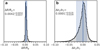 |
Fig. 3 Radius accuracy (a) and k2 accuracy (b) of model 2 after recalculating the planet interior based on the MDN prediction. Panel a shows the distribution in the relative radius error, panel b of the relative k2 error of 10 000 sample points. Blue lines mark the median, with the blue areas showing the range where 80% of values lie. |
Average Hellinger distance  for 20 randomly selected validation planets of all MDN (log-ratio) output distributions and of their corresponding transformed parameters.
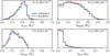 |
Fig. 4 Example of the Hellinger distances for a well-predicted planet (4.722 M⊕, 1.82 R⊕) from the 20 validation planets. The blue line marks the independent validation, the orange line shows the ExoMDN prediction. |
5 Results
5.1 Earth and Neptune
We demonstrate the ability of ExoMDN to perform an interior characterization of Earth and Neptune by treating them as if they were exoplanets, where only the mass and radius are measured, and the equilibrium temperature is set according to their orbital distance. Earth represents the archetypical rocky planet whose internal structure is best known of all the planets in the Solar System. Neptune lies on the upper end of the mass range we investigate and is a representative example of volatile-rich planets.
The MDN prediction takes the form of a six-dimensional distribution of the log-ratios of masses and thicknesses of the planetary layers, which can be transformed back to layer mass and thickness, as described in Sect. 3.5. For clarity, we will focus in this section only on the thickness of the layers. Figures showing the mass fractions can be found in the appendix.
Figure 5 shows the posterior distribution of log-ratios for Earth, as approximated by the MDN, given Earth’s mass, radius, and equilibrium temperature of 255 K. The ellipses in the upper right plots show the location and covariance of each Gaussian kernel, with the colors marking the respective mixture weights, αi. The kernels are well spaced with little overlap and most mixture weights are similar. This indicates that the MDN is able to efficiently leverage all its 50 kernels to construct the posterior distribution.
We sampled 200 000 points from the log-ratio distribution to construct the posterior distribution of the actual layer thickness, which are shown in Fig. 6. Given only three observables (mass, radius, and equilibrium temperature), the prediction indicates a mostly rocky planet composed of an iron core which makes up at least 50% of the planet, and with only little water and gas. The colored symbols mark end-member interior structures with only two layers. In this case, only three of these exist, namely: (1) the actual structure of the Earth with an iron core making up 55% of the interior, and a silicate mantle on top; (2) an iron-water planet composed of a relative core size of 73% and an ice layer; and (3) an iron-gas planet composed of a massive iron core making up 80% of the planet, and a H/He envelope taking up the rest. In cases 2 and 3, the iron core needs to be very large to compensate for the low density of the water and gas layers. Although these two cases are probably not likely to occur in nature, they demonstrate that the interior cannot be fully constrained without additional constraints. In this example, the thickness of the silicate mantle in particular can barely be constrained.
It should be noted that due to our assumption of uniform priors, the most commonly predicted interior structures encompass a combination of all four layers. For this reason, the distributions presented should not be understood as definitive probabilities, but rather as the number of potential solutions for each given layer thickness fraction. Consequently, the actual interior of Earth lies outside the bulk of the predicted distribution. In fact, only a single solution exists that matches Earth’s mass and radius with only an iron core and a silicate mantle, and no water or extended atmosphere.
For Neptune, the MDN predicts a substantial atmosphere between 20 and 70% of the planet’s radius (Fig. 7) and only a small iron core (≤40% of the radius). We note here that rather than the actual temperature of 51 K, we used an equilibrium temperature of 100 K, which is the lowest temperature for which the AQUA EoS used for the water layer is valid. The predicted interior structures lie well within previously published results, which generally agree on Neptune having a small iron-silicate core of about 20% of the planet’s radius and an atmosphere of about 30–40%, with a water-rich envelope in between (e.g., Hubbard et al. 1991; Podolak et al. 1995; Nettelmann et al. 2013; Neuenschwander & Helled 2022).
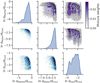 |
Fig. 5 Predicted log-ratios of the thickness of interior layers for an Earth-like planet with 1 M⊕ and 1 R⊕. The ellipses in the top right plots mark the location and covariance of each of the 50 Gaussian kernels, with the colors showing the mixture weight of each kernel. |
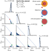 |
Fig. 6 Predicted thickness of interior layers for an Earth-like planet with 1 M⊕ and 1 R⊕. The colored points mark possible end-member compositions, which are illustrated on the right. The red circle corresponds to Earth’s true interior structure. The diagonal plots show the marginal distributions of each layer, with the blue dashed lines marking the median value and the dotted lines the 5th and 95th percentiles. |
5.2 Application to exoplanets
One of the main advantages of using neural networks for interior structure inference over other methods such as MCMC sampling is the speed at which the posterior distribution can be obtained. The inference process for MCMC sampling can take several hours per individual planet (e.g., Haldemann et al. 2023). The MDN can perform the same prediction in fractions of a second. In addition, the MDN model is optimized for bulk processing of inputs owing to the Keras framework, allowing for multiple input samples to be predicted simultaneously. Between 1 and 1000 input data points, we find little difference in the computation time needed by the MDN for a prediction (tMDN, Table 3). The sampling from the predicted distribution and transformation to mass and radius fractions (see. Sect. 3.5) takes up most of the time (tsampling). Even so, predicting and sampling a thousand planets is possible in under six seconds on a conventional laptop processor2. In fact, the main limitation to predicting a large number of planets simultaneously is the amount of available computer memory.
These fast prediction times mean that interior structures can be inferred for every exoplanet for which mass, radius, and equilibrium temperature are known. To demonstrate this, we selected planets from the NASA Exoplanet Archive3 that lie in the parameter space of our training data (Table 1) and for which upper and lower mass and radius uncertainties are given. We used ExoMDN to infer the interior structure of each planet, incorporating the mass, radius, and equilibrium temperature uncertainties according to Sect. 3.6. For each planet, we sampled 5000 mass, radius, and equilibrium temperature points from within a normal distribution given by the uncertainties, and predicted the posterior distribution for each point. From each of these posterior distributions, we then generated an additional ten random samples. In total, this yields 50000 samples of interior structures per planet, forming the full posterior distribution and spanning the range of measurement uncertainties.
Table A.1 shows the 22 planets from this dataset where mass uncertainties are below 10% and radius uncertainties are below 5%. This includes the well studied planets GJ 1214 b, GJ 486 b, and the TRAPPIST-1 planets, among others. For each planet, we provide the predicted median thickness of each interior layer, alongside the ranges in which 90% of the solutions are found. The total time to produce this data was ≈30s. A more extensive data set of 75 planets with radius and mass uncertainties of 10 and 20%, respectively, including both mass fractions and thickness, is available online at the CDS.
Upcoming exoplanet missions such as PLATO (Rauer et al. 2014) will significantly increase the number of exoplanets with well-determined masses and radii. PLATO in particular will allow for the radii of Earth-sized planets to be determined within an accuracy of up to 3%, while follow-up ground based observations are expected to constrain the mass of these planets with an accuracy of 10% or better. We can leverage the fast prediction times of ExoMDN to investigate the degree to which the interior of a planet could be constrained based on the accuracy of the mass and radius determination. Taking Earth and Neptune as examples, we imposed a 10% mass uncertainty and varied the radius uncertainty between 1 and 20% (Fig. 8). As above, in each case we sample 10000 times from within mass and radius uncertainties, and take ten random samples from each predicted posterior distribution for a total of 100 000 samples.
We find that with a radius accuracy of 3%, the core radius fraction of Earth can be constrained to  (error bars are the 5th and 95th percentiles, respectively), which is close to the value we found assuming a perfect knowledge of mass and radius (Fig. 6). With a radius accuracy of 10%, the core size is significantly less well constrained
  . Similarly, with a radius accuracy of 3%, the predicted atmosphere thickness of a Neptune analog (Fig. 8b) is
  , which is again close to the value obtained assuming no error in mass and radius (Fig. 7). With a radius accuracy of 10%, the uncertainty of dGas grows to
  . Increasing the radius accuracy has little effect on the possibility to constrain the layers below the atmosphere. Due to the low density of the atmosphere, different planet radii can be easily accommodated by small changes in atmosphere mass without significantly affecting the other layers. In a sense, the presence of a large atmosphere obscures the inference of the thickness of the deeper layers.
The radius accuracy controls to a large extent the uncertainties in the predicted thickness of the various layers. For completeness, we show in Fig. B.3 predictions of Earth- and Neptune-like interiors obtained when both radius and mass accuracies are varied simultaneously (from 1 to 20% and from 3 to 40%, respectively). Indeed, the inferred structures are very similar to those we obtained by fixing the mass accuracy to 10%.
Average inference time for different numbers of planets.
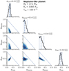 |
Fig. 7 Predicted thickness of interior layers for a Neptune-like planet with 17.1 M⊕ and 3.865 R⊕. The diagonal plots show the marginal distributions of each layer, with the blue dashed lines marking the median value and the dotted lines the 5th and 95 percentiles.(*) Instead of Neptune’s equilibrium temperature of 51 K, a value of 100 K was used to be in line with the parameter range of the training data. |
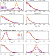 |
Fig. 8 Effect of radius uncertainty, δR, on the ability to constrain the interior for Earth (a) and Neptune (b) analogs. Each panel shows the marginal distributions for each interior layer with increasing amounts of radius uncertainty. An uncertainty of 10% in mass and 2% in Teq has been assumed for both planets in all cases.(*) Instead of Neptune’s equilibrium temperature of 51 K, a value of 100 K was used to be in line with the parameter range of the training data. |
5.3 Constraining the interior with k2
Mass, radius, and equilibrium temperature alone are not sufficient to fully constrain the interior of a planet, as demonstrated above. The fluid Love number k2 is a potential direct link from observation to interior structure, as it only depends on the density distribution in the planet. This stands in contrast to for example the elemental abundances of the host star, which may be representative of the bulk abundances of the planet and its atmosphere (Dorn et al. 2015, 2017a; Brugger et al. 2017; Spaargaren et al. 2020), but which necessitate additional assumptions about the planet formation and evolution history.
Figure 9 shows the MDN prediction of the interior of Earth, given knowledge of Earth’s value of k2 = 0.933 (Lambeck 1980). With this added information, the MDN is capable of fully constraining Earth’s actual interior (particular in comparison to Fig. 6). In fact, the constraints from k2 are strong enough that the composition of the iron core becomes important. The planets in the training data are modeled with a pure iron core, while Earth has about 10–15 wt.% of lighter elements in its core (Poirier 1994). Thus, the MDN predicts a smaller core radius of 51%, while the true core size is about 54.5% of the total radius. In practice, of course, the measurements k2 for exoplanets will be associated with considerable uncertainties. Constraining a planet’s interior to the degree shown in Fig. 9 is therefore unlikely in the near future. Nevertheless, we can utilize the fast predictions of the MDN to estimate the accuracy that would be needed to properly constrain the interior. We performed a number of predictions for Earth and Neptune analogs with increasing k2 uncertainties, in addition to mass, radius, and equilibrium temperature uncertainties of 5, 3, and 2%, respectively). These values are representative of a very well studied and characterized exoplanet, which would likely be needed for an accurate measurement of the Love number. For Neptune, we take a value of k2 = 0.392, which we calculated after Hubbard (1984) from the gravitational moment J2 = 3.408 43 × 10−3 (Jacobson 2009). The predicted results are detailed in Fig. 10. As the uncertainty in k2 grows, the interior of both planets becomes less and less constrained. We find that with a k2 uncertainty of 10%, Earth’s core and mantle thickness could be constrained to about ±13% of their actual value (within the 5 and 95% percentiles). With a k2 uncertainty of 20%, mantle and core can be constrained to within ±17%. Even with large k2 uncertainties, Earth could be clearly identified as a rocky planet with very little water and a thin atmosphere. The uncertainties of mass and radius put a limit on how well the interior can be determined. With the given mass and radius uncertainties, we find that in the Earth-like case, k2 uncertainties lower than 10% do not constrain the interior further. For Neptune, a 10% uncertainty in k2 could help constrain the atmospheric thickness to  of the planet’s radius.
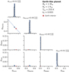 |
Fig. 9 Predicted thickness of interior layers for an Earth-like planet with 1 M⊕ and 1 R⊕, where also k2 is known (k2 = 0.933) in addition to mass and radius. The red circle marks Earth’s true interior structure. The diagonal plots show the marginal distributions of each layer, with the blue dashed lines marking the median value and the dotted lines the 5th and 95th percentiles. Compared to Fig. 6, the axis limits have been adjusted to better show the model results. |
6 Discussion and conclusions
MDNs can provide a reliable way to rapidly characterize the interior structure of exoplanets within fractions of a second. Compositional data such as mass fractions of individual interior layers can be easily accommodated in the network by using log-ratio transformations. An additional benefit of a machine learning approach over other inference methods is that the forward model computations are decoupled from the actual inference process. The training data are calculated separately before training and the training process encodes the information from the training data into the network weights. The trained network itself is standalone and interior inferences can be performed without requiring the training data, a dedicated interior model, a separate inference scheme, or prior expertise about exoplanet interior modeling. This stands in contrast to MCMC sampling, where running the data-generating forward model during the inference is an integral part of exploring the posterior distributions.
While in this work the training data were generated from a single forward model, this is actually not necessary for the training of the network. Since the forward model data generation is separated from the inference itself, different parts of the data set can be modeled by different dedicated forward models, for example to include both Jupiter-like and low-mass planets which may require different modeling approaches. Importantly, this means that the training data can be computed, collected, and combined from multiple sources without much overhead and without the need to integrate different numerical codes into a single model, as would be needed for MCMC sampling. Furthermore, this means that this method is easily extendable to different models and applicable to other inverse problems. However, the necessary prior generation of training data locks the model assumptions of the forward model into the training data. Changing the forward model therefore requires computing a new set of training data and training of a new neural network. This may be a drawback if the forward model assumptions often change (e.g., with different atmosphere compositions).
Our method is best suited for problems where the number of constraining parameters is relatively small. The required number of training samples increases (potentially exponentially) with each additional parameter, a phenomenon which has been termed the “curse of dimensionality” (Bellman 1966). This can make the generation and handling of training data cumbersome and time-consuming for larger numbers of constraining parameters, as it is generally necessary to sample from the entire investigated parameter space to achieve good MDN performance. A potential way to alleviate this issue could be to generate the training data “on the fly” and train the network with an incremental learning approach (van de Ven et al. 2022), where the network learns continuously with new incoming data, thus reducing the need to save large amounts of data.
Conditional invertible neural networks (cINN) may be another alternative, as demonstrated by Haldemann et al. (2023). These potentially work better with higher-dimensional data while requiring comparatively less training data, with the tradeoff that the network setup is more complex and predictions are generally slower.
As with other machine learning methods, the nature of the training process introduces a small amount of intrinsic noise into the model. However, we have shown that the errors introduced by this are generally small (see Sect. 4.1), particularly for exoplanets where uncertainties in the observable quantities are relatively large.
The file size of the fully trained model is only 4 ≈ 6.8 MB, which facilitates sharing and distribution online. The posterior distributions predicted by ExoMDN provide a first characterization of newly observed planets, which can then be further explored with dedicated models. ExoMDNs posterior distributions could also be employed as advanced priors for MCMC inferences based on more sophisticated forward models to help speed up their convergence. We believe that ExoMDN is a valuable tool for the exoplanet science community to gain access to a rapid first characterization of the possible interiors of low-mass planets.
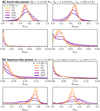 |
Fig. 10 Effect of k2 uncertainty on the ability to constrain the interior for Earth (a) and Neptune (b) analogs. Each panel shows the marginal distributions for each interior layer with increasing amounts of k2 uncertainty. An uncertainty of 5 in mass, 3 in radius, and 2% in Teq has been assumed for both planets in all cases.(*) Instead of Neptune’s equilibrium temperature of 51 K, a value of 100 K was used to be in line with the parameter range of the training data. |
All predictions were performed on an Intel® Core™ i5-8250U CPU.
Acknowledgements
We thank Heike Rauer for important suggestions and discussions on the role of uncertainties in mass and radius, and an anonymous referee for their comments, which helped improve a previous version of the manuscript. We acknowledge the support of the DFG priority program SPP 1992 “Exploring the Diversity of Extrasolar Planets” (TO 704/3-1) and of the research unit FOR 2440 “Matter under planetary interior conditions” (PA 3689/1-1). Training of ExoMDN was performed on a GPU Workstation also sponsored by the DFG research unit FOR 2440 (grant number RE 882/19-2), which is gratefully acknowledged.
Appendix A Exoplanet predictions
Predicted thicknesses di of interior layers for exoplanets with well known masses and radii.
Appendix B Additional figures
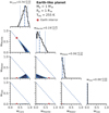 |
Fig. B.1 Predicted mass fraction of interior layers for an Earth-like planet with 1 M⊕ and 1 R⊕. The red circle corresponds to Earth’s true interior structure. Due to the presence of lighter elements in Earth’s core, the actual core mass of Earth 33% is slightly lower than what is predicted by ExoMDN for a solution with no water and atmosphere (39%). The diagonal plots show the marginal distributions of each layer, with the blue dashed lines marking the median value and the dotted lines the 5th and 95th percentiles. |
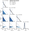 |
Fig. B.2 Predicted mass fraction of interior layers for a Neptune-like planet with 17.1 M⊕ and 3.865 R⊕. The diagonal plots show the marginal distributions of each layer, with the blue dashed lines marking the median value and the dotted lines the 5th and 95th percentiles.(*) Instead of Neptune’s equilibrium temperature of 51 K, a value of 100 K was used to be in line with the parameter range of the training data. |
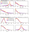 |
Fig. B.3 Effect of radius (δR) and mass (δM) uncertainty on the ability to constrain the interior for Earth (a) and Neptune (b) analogs. Each panel shows the marginal distributions for each interior layer with increasing amounts of radius and mass uncertainty. A Teq uncertainty of 2% has been assumed for both planets.(*) Instead of Neptune’s equilibrium temperature of 51 K, a value of 100 K was used to be in line with the parameter range of the training data. |
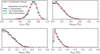 |
Fig. B.4 Comparison of the two possible approaches to incorporate measurement uncertainties (Sect. 3.6) for an Earth-like planet with 5% radius and 10% mass uncertainty. 5000 posterior distributions were predicted from random mass, radius, and Teq inputs within the uncertainties. The red line shows the predicted thickness of each interior layer obtained by first summing up all 5000 posterior distributions and then taking 5000 random samples from the combined mixture, while the dark blue, light blue, and green lines show those obtained by first taking 1, 10, and 100 samples, respectively, from each of the 5000 posteriors and then combining the samples. |
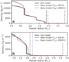 |
Fig. B.5 Illustration of the differences in interior models between the previous work (Baumeister et al. 2020, black line) and this work (blue and red lines, for two different equilibrium temperatures Teq = 100K and Teq = 1000K, respectively). The figure shows density profiles of a representative 5 M⊕ planet with wCore = 0.2, wMantle = 0.49, wWater = 0.3, and wGas = 0.01 (Panel a). Panel b shows a zoomed-in view of only the water and atmosphere layers. The dashed lines mark the respective planets’ radii. |
References
- Abadi, M., Agarwal, A., Barham, P., et al. 2016, ArXiv e-prints [arXiv:1603.04467] [Google Scholar]
- Acuña, L., Deleuil, M., Mousis, O., et al. 2021, A&A, 647, A53 [NASA ADS] [CrossRef] [EDP Sciences] [Google Scholar]
- Agarwal, S., Tosi, N., Kessel, P., Breuer, D., & Montavon, G. 2021a, Phys. Rev. Fluids, 6, 113801 [NASA ADS] [CrossRef] [Google Scholar]
- Agarwal, S., Tosi, N., Kessel, P., et al. 2021b, Earth and Space Science, 8, 4 [CrossRef] [Google Scholar]
- Aitchison, J. 1982, J. R. Stat. Soc. Ser. B Methodol., 44, 139 [Google Scholar]
- Akinsanmi, B., Barros, S. C. C., Santos, N. C., et al. 2019, A&A, 621, A117 [NASA ADS] [CrossRef] [EDP Sciences] [Google Scholar]
- Alibert, Y., & Venturini, J. 2019, A&A, 626, A21 [NASA ADS] [CrossRef] [EDP Sciences] [Google Scholar]
- Atkins, S., Valentine, A. P., Tackley, P. J., & Trampert, J. 2016, Phys. Earth Planet. Int., 257, 171 [CrossRef] [Google Scholar]
- Auddy, S., Dey, R., Lin, M.-K., Carrera, D., & Simon, J. B. 2022, ApJ, 936, 93 [NASA ADS] [CrossRef] [Google Scholar]
- Baumeister, P., Padovan, S., Tosi, N., et al. 2020, ApJ, 889, 42 [Google Scholar]
- Bellman, R. 1966, Science, 153, 34 [NASA ADS] [CrossRef] [Google Scholar]
- Bishop, C. M. 1994, Mixture Density Networks, Tech. Rep., Aston University [Google Scholar]
- Bouchet, J., Mazevet, S., Morard, G., Guyot, F., & Musella, R. 2013, Phys. Rev. B, 87, 094102 [Google Scholar]
- Brando, A. 2017, Master’s Thesis, Universitat Politecnica de Catalunya, Spain [Google Scholar]
- Brugger, B., Mousis, O., Deleuil, M., & Deschamps, F. 2017, ApJ, 850, 93 [NASA ADS] [CrossRef] [Google Scholar]
- Cambioni, S., Asphaug, E., Emsenhuber, A., et al. 2019, ApJ, 875, 40 [NASA ADS] [CrossRef] [Google Scholar]
- Chaushev, A., Raynard, L., Goad, M. R., et al. 2019, MNRAS, 488, 5232 [Google Scholar]
- Chollet, F. et al. 2015, Keras, https://keras.io/ [Google Scholar]
- Csizmadia, Sz., Hellard, H., & Smith, A. M. S. 2019, A&A, 623, A45 [NASA ADS] [CrossRef] [EDP Sciences] [Google Scholar]
- Dorn, C., & Heng, K. 2018, ApJ, 853, 64 [Google Scholar]
- Dorn, C., Khan, A., Heng, K., et al. 2015, A&A, 577, A83 [NASA ADS] [CrossRef] [EDP Sciences] [Google Scholar]
- Dorn, C., Hinkel, N. R., & Venturini, J. 2017a, A&A, 597, A38 [NASA ADS] [CrossRef] [EDP Sciences] [Google Scholar]
- Dorn, C., Venturini, J., Khan, A., et al. 2017b, A&A, 597, A37 [NASA ADS] [CrossRef] [EDP Sciences] [Google Scholar]
- Emsenhuber, A., Cambioni, S., Asphaug, E., et al. 2020, ApJ, 891, 6 [NASA ADS] [CrossRef] [Google Scholar]
- Fortney, J. J., Marley, M. S., & Barnes, J. W. 2007, ApJ, 659, 1661 [Google Scholar]
- Goodfellow, I., Bengio, Y., & Courville, A. 2017, Deep Learning (Cambridge: MIT Press) [Google Scholar]
- Guillot, T. 2010, A&A, 520, A27 [NASA ADS] [CrossRef] [EDP Sciences] [Google Scholar]
- Hakim, K., Rivolidini, A., Van Hoolst, T., et al. 2018, Icarus, 313, 61 [NASA ADS] [CrossRef] [Google Scholar]
- Haldemann, J., Alibert, Y., Mordasini, C., & Benz, W. 2020, A&A, 643, A105 [NASA ADS] [CrossRef] [EDP Sciences] [Google Scholar]
- Haldemann, J., Ksoll, V., Walter, D., et al. 2023, A&A, 672, A180 [NASA ADS] [CrossRef] [EDP Sciences] [Google Scholar]
- Hellard, H., Csizmadia, S., Padovan, S., et al. 2019, ApJ, 878, 119 [NASA ADS] [CrossRef] [Google Scholar]
- Himes, M. D., Harrington, J., Cobb, A. D., et al. 2022, Planet. Sci. J., 3, 91 [NASA ADS] [CrossRef] [Google Scholar]
- Hinkel, N. R., & Unterborn, C. T. 2018, ApJ, 853, 83 [NASA ADS] [CrossRef] [Google Scholar]
- Hirose, K., Wood, B., & Vočadlo, L. 2021, Nat. Rev. Earth Environ., 2, 645 [NASA ADS] [CrossRef] [Google Scholar]
- Holland, T. J. B., & Powell, R. 2011, J. Metamorph. Geol., 29, 333 [Google Scholar]
- Huang, C., Rice, D. R., & Steffen, J. H. 2022, MNRAS, 513, 5256 [NASA ADS] [CrossRef] [Google Scholar]
- Hubbard, W. B. 1984, Planetary Interiors (New York, N.Y.: Van Nostrand Reinhold) [Google Scholar]
- Hubbard, W. B., Nellis, W. J., Mitchell, A. C., et al. 1991, Science, 253, 648 [NASA ADS] [CrossRef] [Google Scholar]
- Jacobson, R. A. 2009, AJ, 137, 4322 [Google Scholar]
- Jontof-Hutter, D. 2019, Ann. Rev. Earth Planet. Sci., 47, 141 [Google Scholar]
- Kellermann, C., Becker, A., & Redmer, R. 2018, A&A, 615, A39 [NASA ADS] [CrossRef] [EDP Sciences] [Google Scholar]
- Lambeck, K. 1980, The Earth’s Variable Rotation: Geophysical Causes and Con- sequences, Cambridge Monographs on Mechanics (Cambridge: Cambridge University Press) [CrossRef] [Google Scholar]
- Leconte, J., & Chabrier, G. 2012, A&A, 540, A20 [NASA ADS] [CrossRef] [EDP Sciences] [Google Scholar]
- MacKenzie, J., Grenfell, J. L., Baumeister, P., et al. 2023, A&A, 671, A65 [NASA ADS] [CrossRef] [EDP Sciences] [Google Scholar]
- Malik, A., Moster, B. P., & Obermeier, C. 2021, MNRAS, 513, 5505 [NASA ADS] [Google Scholar]
- Márquez-Neila, P., Fisher, C., Sznitman, R., & Heng, K. 2018, Nat. Astron., 2, 719 [CrossRef] [Google Scholar]
- Martin, C., & Duhaime, D. 2019, https://zenodo.org/record/2578015 [Google Scholar]
- Nair, V., & Hinton, G. E. 2010, in Proceedings of the 27th International Conference on International Conference on Machine Learning, ICML’10 (Omnipress), 807 [Google Scholar]
- Nettelmann, N., Fortney, J. J., Kramm, U., & Redmer, R. 2011, ApJ, 733, 2 [NASA ADS] [CrossRef] [Google Scholar]
- Nettelmann, N., Helled, R., Fortney, J. J., & Redmer, R. 2013, Planet. Space Sci., 77, 143 [Google Scholar]
- Neuenschwander, B. A., & Helled, R. 2022, MNRAS, 512, 3124 [CrossRef] [Google Scholar]
- O’Malley, T., Bursztein, E., Long, J., et al. 2019, https://github.com/keras-team/keras-tuner [Google Scholar]
- Padovan, S., Spohn, T., Baumeister, P., et al. 2018, A&A, 620, A178 [NASA ADS] [CrossRef] [EDP Sciences] [Google Scholar]
- Pawlowsky-Glahn, V., & Egozcue, J. J. 2006, Geol. Soc. London Spec. Pub., 264, 1 [NASA ADS] [CrossRef] [Google Scholar]
- Plotnykov, M., & Valencia, D. 2020, MNRAS, 499, 932 [CrossRef] [Google Scholar]
- Podolak, M., Weizman, A., & Marley, M. 1995, Planet. Space Sci., 43, 1517 [NASA ADS] [CrossRef] [Google Scholar]
- Poirier, J.-P. 1994, Phys. Earth Planet. Interiors, 85, 319 [NASA ADS] [CrossRef] [Google Scholar]
- Rauer, H., Catala, C., Aerts, C., et al. 2014, Exp. Astron., 38, 249 [Google Scholar]
- Rogers, L. A., & Seager, S. 2010, ApJ, 712, 974 [Google Scholar]
- Saumon, D., Chabrier, G., & van Horn, H. M. 1995, ApJS, 99, 713 [NASA ADS] [CrossRef] [Google Scholar]
- Seager, S., Kuchner, M., Hier-Majumder, C., & Militzer, B. 2007, ApJ, 669, 1279 [Google Scholar]
- Sotin, C., Grasset, O., & Mocquet, A. 2007, Icarus, 191, 337 [Google Scholar]
- Spaargaren, R. J., Ballmer, M. D., Bower, D. J., Dorn, C., & Tackley, P. J. 2020, A&A, 643, A44 [NASA ADS] [CrossRef] [EDP Sciences] [Google Scholar]
- Spiegel, D. S., Fortney, J. J., & Sotin, C. 2014, Proc. Natl. Acad. Sci., 111, 12622 [NASA ADS] [CrossRef] [Google Scholar]
- Tateno, S., Hirose, K., Sata, N., & Ohishi, Y. 2009, Earth Planet. Sci. Lett., 277, 130 [CrossRef] [Google Scholar]
- Unterborn, C. T., & Panero, W. R. 2019, J. Geophys. Res. Planets, 124, 1704 [NASA ADS] [CrossRef] [Google Scholar]
- Valencia, D., Sasselov, D. D., & O’Connell, R. J. 2007, ApJ, 665, 1413 [Google Scholar]
- Valizadegan, H., Martinho, M. J. S., Wilkens, L. S., et al. 2022, ApJ, 926, 120 [NASA ADS] [CrossRef] [Google Scholar]
- van de Ven, G. M., Tuytelaars, T., & Tolias, A. S. 2022, Nat. Mach. Intell., 4, 1185 [CrossRef] [Google Scholar]
- Van Hoolst, T., Noack, L., & Rivoldini, A. 2019, Adv. Phys. X, 4, 1630316 [NASA ADS] [Google Scholar]
- Wagner, F., Sohl, F., Hussmann, H., Grott, M., & Rauer, H. 2011, Icarus, 214, 366 [Google Scholar]
- Zeng, L., & Sasselov, D. 2013, PASP, 125, 227 [Google Scholar]
- Zeng, L., Jacobsen, S. B., Sasselov, D. D., et al. 2019, Proceedings of the Natl. Acad. Sci., 116, 9723 [NASA ADS] [CrossRef] [Google Scholar]
- Zhao, Y., & Ni, D. 2021, A&A, 650, A177 [NASA ADS] [CrossRef] [EDP Sciences] [Google Scholar]
- Zingales, T., & Waldmann, I. P. 2018, AJ, 156, 268 [NASA ADS] [CrossRef] [Google Scholar]
All Tables
Average Hellinger distance for 20 randomly selected validation planets of all MDN (log-ratio) output distributions and of their corresponding transformed parameters.
Predicted thicknesses di of interior layers for exoplanets with well known masses and radii.
All Figures
|
Fig. 1 Schematic overview of the MDN architecture and inference procedure. |
| In the text | |
|
Fig. 2 Radius accuracy of Model 1 after recalculating the planet interior based on the MDN prediction. Panel a shows the distribution of the relative radius error of 10000 sample points. The blue line marks the median, with the blue area showing the range where 80% of values lie. Panels b–e show the standard deviation in relative radius errors σ for a variety of planet parameters: bulk density (b), planet mass (c), equilibrium temperature (d), and average atmosphere thickness |
| In the text | |
|
Fig. 3 Radius accuracy (a) and k2 accuracy (b) of model 2 after recalculating the planet interior based on the MDN prediction. Panel a shows the distribution in the relative radius error, panel b of the relative k2 error of 10 000 sample points. Blue lines mark the median, with the blue areas showing the range where 80% of values lie. |
| In the text | |
|
Fig. 4 Example of the Hellinger distances for a well-predicted planet (4.722 M⊕, 1.82 R⊕) from the 20 validation planets. The blue line marks the independent validation, the orange line shows the ExoMDN prediction. |
| In the text | |
|
Fig. 5 Predicted log-ratios of the thickness of interior layers for an Earth-like planet with 1 M⊕ and 1 R⊕. The ellipses in the top right plots mark the location and covariance of each of the 50 Gaussian kernels, with the colors showing the mixture weight of each kernel. |
| In the text | |
|
Fig. 6 Predicted thickness of interior layers for an Earth-like planet with 1 M⊕ and 1 R⊕. The colored points mark possible end-member compositions, which are illustrated on the right. The red circle corresponds to Earth’s true interior structure. The diagonal plots show the marginal distributions of each layer, with the blue dashed lines marking the median value and the dotted lines the 5th and 95th percentiles. |
| In the text | |
|
Fig. 7 Predicted thickness of interior layers for a Neptune-like planet with 17.1 M⊕ and 3.865 R⊕. The diagonal plots show the marginal distributions of each layer, with the blue dashed lines marking the median value and the dotted lines the 5th and 95 percentiles.(*) Instead of Neptune’s equilibrium temperature of 51 K, a value of 100 K was used to be in line with the parameter range of the training data. |
| In the text | |
|
Fig. 8 Effect of radius uncertainty, δR, on the ability to constrain the interior for Earth (a) and Neptune (b) analogs. Each panel shows the marginal distributions for each interior layer with increasing amounts of radius uncertainty. An uncertainty of 10% in mass and 2% in Teq has been assumed for both planets in all cases.(*) Instead of Neptune’s equilibrium temperature of 51 K, a value of 100 K was used to be in line with the parameter range of the training data. |
| In the text | |
|
Fig. 9 Predicted thickness of interior layers for an Earth-like planet with 1 M⊕ and 1 R⊕, where also k2 is known (k2 = 0.933) in addition to mass and radius. The red circle marks Earth’s true interior structure. The diagonal plots show the marginal distributions of each layer, with the blue dashed lines marking the median value and the dotted lines the 5th and 95th percentiles. Compared to Fig. 6, the axis limits have been adjusted to better show the model results. |
| In the text | |
|
Fig. 10 Effect of k2 uncertainty on the ability to constrain the interior for Earth (a) and Neptune (b) analogs. Each panel shows the marginal distributions for each interior layer with increasing amounts of k2 uncertainty. An uncertainty of 5 in mass, 3 in radius, and 2% in Teq has been assumed for both planets in all cases.(*) Instead of Neptune’s equilibrium temperature of 51 K, a value of 100 K was used to be in line with the parameter range of the training data. |
| In the text | |
|
Fig. B.1 Predicted mass fraction of interior layers for an Earth-like planet with 1 M⊕ and 1 R⊕. The red circle corresponds to Earth’s true interior structure. Due to the presence of lighter elements in Earth’s core, the actual core mass of Earth 33% is slightly lower than what is predicted by ExoMDN for a solution with no water and atmosphere (39%). The diagonal plots show the marginal distributions of each layer, with the blue dashed lines marking the median value and the dotted lines the 5th and 95th percentiles. |
| In the text | |
|
Fig. B.2 Predicted mass fraction of interior layers for a Neptune-like planet with 17.1 M⊕ and 3.865 R⊕. The diagonal plots show the marginal distributions of each layer, with the blue dashed lines marking the median value and the dotted lines the 5th and 95th percentiles.(*) Instead of Neptune’s equilibrium temperature of 51 K, a value of 100 K was used to be in line with the parameter range of the training data. |
| In the text | |
|
Fig. B.3 Effect of radius (δR) and mass (δM) uncertainty on the ability to constrain the interior for Earth (a) and Neptune (b) analogs. Each panel shows the marginal distributions for each interior layer with increasing amounts of radius and mass uncertainty. A Teq uncertainty of 2% has been assumed for both planets.(*) Instead of Neptune’s equilibrium temperature of 51 K, a value of 100 K was used to be in line with the parameter range of the training data. |
| In the text | |
|
Fig. B.4 Comparison of the two possible approaches to incorporate measurement uncertainties (Sect. 3.6) for an Earth-like planet with 5% radius and 10% mass uncertainty. 5000 posterior distributions were predicted from random mass, radius, and Teq inputs within the uncertainties. The red line shows the predicted thickness of each interior layer obtained by first summing up all 5000 posterior distributions and then taking 5000 random samples from the combined mixture, while the dark blue, light blue, and green lines show those obtained by first taking 1, 10, and 100 samples, respectively, from each of the 5000 posteriors and then combining the samples. |
| In the text | |
|
Fig. B.5 Illustration of the differences in interior models between the previous work (Baumeister et al. 2020, black line) and this work (blue and red lines, for two different equilibrium temperatures Teq = 100K and Teq = 1000K, respectively). The figure shows density profiles of a representative 5 M⊕ planet with wCore = 0.2, wMantle = 0.49, wWater = 0.3, and wGas = 0.01 (Panel a). Panel b shows a zoomed-in view of only the water and atmosphere layers. The dashed lines mark the respective planets’ radii. |
| In the text | |
Current usage metrics show cumulative count of Article Views (full-text article views including HTML views, PDF and ePub downloads, according to the available data) and Abstracts Views on Vision4Press platform.
Data correspond to usage on the plateform after 2015. The current usage metrics is available 48-96 hours after online publication and is updated daily on week days.
Initial download of the metrics may take a while.