| Issue |
A&A
Volume 688, August 2024
|
|
|---|---|---|
| Article Number | A103 | |
| Number of page(s) | 13 | |
| Section | Planets and planetary systems | |
| DOI | https://doi.org/10.1051/0004-6361/202450177 | |
| Published online | 07 August 2024 | |
Formation of planetary atmospheres
Analytical estimation of vapor production via planetary impacts
Department of Physics, Graduate School of Science, Nagoya University,
Furo-cho, Chikusa-ku,
Nagoya
464-8602,
Japan
e-mail: This email address is being protected from spambots. You need JavaScript enabled to view it.
; This email address is being protected from spambots. You need JavaScript enabled to view it.
Received:
29
March
2024
Accepted:
16
May
2024
Abstract
To investigate impact vaporization for planetary atmosphere formation, we have studied the thermodynamic state generated by the shock wave due to a high-velocity impact, called the shock field. We have carried out iSALE simulations for high-velocity vertical impacts using ANEOS for an equation-of-state (EoS) model. To understand the shock fields obtained from simulations, we have investigated the contribution of the thermal and cold terms in the EoS model on the Hugoniot curves. Although the thermal and cold terms are important for the pressure, the internal energy is mainly determined by the thermal term. We thus assume a simple EoS determined by the thermal term and then analytically derive the shock internal-energy field, which reproduces the results of simulations well. Using the analytical solution of internal energy and the Hugoniot curve, we have derived the shock pressure field analytically as well. The analytical solutions for internal energy and pressure are valid even for impact velocities as low as the sound speed. The solution is good for the vertical direction or within the angles of about 60 degrees. We have applied the solution to impact vaporization for the formation of planetary atmospheres. This gives good estimation of reformation of the planetary atmospheres of Earth sized planet.
Key words: equation of state / hydrodynamics / shock waves / planets and satellites: atmospheres / planets and satellites: interiors
© The Authors 2024
 Open Access article, published by EDP Sciences, under the terms of the Creative Commons Attribution License (https://creativecommons.org/licenses/by/4.0), which permits unrestricted use, distribution, and reproduction in any medium, provided the original work is properly cited.
This article is published in open access under the Subscribe to Open model. This email address is being protected from spambots. You need JavaScript enabled to view it. to support open access publication.
1 Introduction
Planetary impacts are one of the most common phenomena in planet formation. As planetary bodies grow via collisions, their gravitational accelerations are strong, and impact velocities then exceed the sound speed for planet-sized bodies. Such a hyper-velocity impact generates a shock wave, and this shock wave propagates through the planetary bodies, resulting in irreversible heating and compression. The extreme temperature increase causes melting and vaporization of the bodies and, as a consequence, high-speed impacts have produced planetary oceans and atmospheres (e.g., Lange & Ahrens 1982; Melosh & Vickery 1989; Tonks & Melosh 1993). The amount of melt and vapor production is derived from the maximum pressure distribution formed by the shock wave, called the shock pressure field (e.g., Ahrens & O’Keefe 1972; Stewart et al. 2008; Kraus et al. 2015). In addition, the shock pressure field is important for impact disruption and cratering of planetary bodies (Mizutani et al. 1990; Genda et al. 2015; Suetsugu et al. 2018). The collisional outcomes affect planet formation and the collisional evolution of small bodies (Kobayashi & Tanaka 2010; Kobayashi et al. 2010, 2011). Therefore, the shock pressure field is important for understanding phase transition and cratering due to collisions.
Impact vaporization has been investigated via experimental approaches (e.g., Kadono et al. 2002), only a limited range of impact velocities have been tested. On the other hand, the shock pressure profiles have been thoroughly tested in theoretical studies over a wide velocity range using analytical methods (Croft 1982; Melosh 1989; Tonks & Melosh 1993) and numerical simulations (Ahrens & O’keefe 1977; Pierazzo et al. 1995, 1997; Pierazzo & Melosh 2000; Kraus et al. 2011; Monteux & Arkani-Hamed 2016, 2019).
Impact simulations show that the shock pressure field is determined as follows. In an impact event, the region of highest pressure forms around the impact site. Such a nearly isobaric region in a target is called the isobaric core. The shock pressure then decreases with distance from the impact point due to the shock propagation. The pressure decrease can be approximated as a power-law function of a radial distance from the core center. Croft (1982) implemented a semi-analytical model to express the decreasing shock pressure P as a function of radial distance R;
 (1)
(1)
where P0 is the pressure in the isobaric core and Ric is its radius. Although the exponent α has been thoroughly investigated using numerical simulations (e.g., Ahrens & O’keefe 1977; Pierazzo et al. 1997; Kraus et al. 2011; Monteux & Arkani-Hamed 2016, 2019), the exponent depends on the equation of state (EoS) and has huge uncertainty with ranges from 1 to 3.
In impact simulations, the exponents a of shock-pressure profiles depend on materials, and the dependence mainly comes from solid EoS models. One of the most sophisticated solid EoS models is M-ANEOS (Thompson & Lauson 1972; Melosh 2007; Thompson et al. 2019), which is written using analytic formulae with 44 parameters. It has been difficult to theoretically understand the material dependence of the shock-pressure profile given this high number of parameters in complicated formulae.
In this paper, we present an investigation of the shock-pressure field via numerical simulations and analytical methods. We perform simulations for vertical impacts between solid bodies via iSALE with ANEOS. To understand the shock-pressure profile, we also investigate the shock internal-energy profile. We evaluate the contribution of cold and thermal terms in ANEOS to pressure and internal energy. We then analytically derive the shock-pressure profile under the assumption based on the result. Section 2 provides a description of the solid EoS model, the setup for numerical simulations, and the Hugoniot curves used to determine the shocked state. In Sect. 3, we show the results of impact simulations for the shock pressure and internal-energy profiles. We also present the justification for our assumption for the derivation of analytical solutions based on the difference between those values. In Sect. 4, we show how we derive the analytical solutions for the isobaric and decay regions in shocked profiles. In Sect. 5, we discuss the dependence of the shock pressure on the direction of the wave propagation in the target. In Sect. 6, we show how we use our solutions to calculate the amount of vapor in an impact event as a function of impact velocity, and then how we use estimate of vapor to calculate the reformation of the atmosphere removed by a giant impact. We summarize our findings in Sect. 7.
2 Methods
2.1 Solid EoS model: ANEOS
The ANEOS model is widely used in planetary studies (e.g., Pierazzo et al. 1997; Melosh 2007; Kraus et al. 2011). For impact simulations, we use the EoS table in the ANEOS model, which is designed by FORTRAN code.
The ANEOS model provides pressure from the Helmholtz free energy, and the free energy is composed of three terms, as follows:
 (2)
(2)
The first term on the right-hand side in Eq. (2), Fc, the so-called the cold term, depends only on density, and is particular to solid materials and originates from interaction between component particles of the body. The second term Ft is the thermal term, and comes from kinetic energy of the component particles. The third term Fe is provided to represent the pressure of the ionized electrons generated because of the high-temperature and low-density field; it has a minor effect here because temperatures in typical planetary events are much lower than the ionization temperature (Melosh 2007).
2.2 Simulation setup
The ANEOS model needs a set of input parameters and we use parameter sets for water ice (Turtle & Pierazzo 2001) and basalt (Pierazzo et al. 2005). We consider impact simulations between the same materials (ice-ice or basalt-basalt). Planetary impacts are oblique in general. However, we perform numerical simulations of vertical impacts, because we focus on the shock physics determining the shock pressure field. We consider collisions between spherical bodies. However, target bodies are much larger than projectile bodies. Target bodies are thus represented by slabs in simulations.
The shock pressure field caused in an impact event is calculated with the widely used Lagrangian-Eulerian finite-volume shock physics code iSALE-2D (Amsden et al. 1980; Ivanov et al. 1997; Wünnemann et al. 2006). We consider the material initial temperature is 150 K. The projectile radius Rp is 500 m in all simulations. The gravitational force is not included, which is a minor effect for the shock-pressure field.
The iSALE calculation includes Lagrangian tracer particles, and these particles are placed in each cell to record the thermo-dynamic state as a function of position and time. We investigate the shock pressure fields using the tracer particles.
The shock pressure fields obtained from simulations depend on their resolution. In iSALE, the resolution is determined by the cells per projectile radius (cppr). To find a proper resolution, we perform simulations with 20 and 50 cppr (Fig. 1). The maximum pressures for 20 cppr are smaller than those for 50 cppr, because low-resolution simulations weaken shock waves numerically. However, the errors for 20 cppr are within 10% underestimation. To minimize computational time, a fixed resolution of 20 cppr is used in the following simulations.
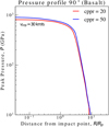 |
Fig. 1 Maximum pressure distribution caused by an impact, also called the shock pressure field, for basalt bodies with an impact speed of 30 km−1. The red curve is the result for 20 cppr, while the blue curve is for 50 cppr. |
3 Numerical results
3.1 Examples of impact simulation
Figure 2 shows the pressure and internal-energy profiles at t/ts = 0, 1, and 4 obtained from an iSALE impact simulation with an impact velocity of amp = 30 km s−1 between icy bodies, where t is the time from the collision, ts = 2Rp/υimp, and Rp is the radius of the projectile body. The shock wave significantly increases the pressure and internal energy around |R| ≲ 2 and z ∽ −1 at t = ts (Fig. 2b), where R is the distance from the symmetric pole and z is the height from the target surface. The shock wave widely propagates and moderately increases the pressure and internal energy at t = 4ts (Fig. 2c), which shows the decay of the shock wave.
The shock pressure field as shown in Fig. 1 is determined by the shock propagation. Pressure reaches a maximum value just after the shock wave has passed. In the early stage, the pressure and internal energy increase around the impact point (Fig. 2b), while its elevation becomes smaller in a region more distant from the impact point in the later stage (Fig. 2c). The maximum values of pressure and internal energy are recorded by tracer particles. Figure 1 is plotted for the shock pressure field along with impact direction, which is shown with a white arrow in Fig. 2a. In the following sections, we show the vertical shock field for pressure and internal energy. We discuss the direction dependence in Sect. 5.
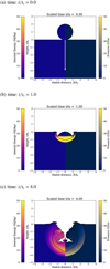 |
Fig. 2 Result of the iSALE simulation. The changes to pressure and the internal energy caused by an impact shock with υimp = 30 km s−1 are illustrated as a function of position at t = 0 (a), t = ts (b), and t = 4ts (c). Calculation time is scaled by the time ts, where ts = 2Rp/υimp. |
3.2 Shock pressure fields
Melting and vaporization in an impact event are governed only by the thermodynamic state of the materials formed by shock propagation if the expansion process following shock compression can be assumed to be an adiabatic process. In particular, the shock pressure field has been well investigated because of its importance in the determination of melting, vaporization, and crater size (e.g., Pierazzo et al. 1997; Kraus et al. 2011).
Figure 3 shows the shock pressure fields with distance from the impact point for impacts between icy or basaltic bodies with various impact velocities. The peak pressure is almost the same for R ≲ 2RV around the impact point, which is called the isobaric core. For R >> Rp, the peak pressure decreases with distance, which is approximated as a power-law function of R.
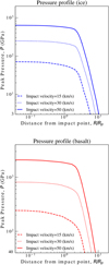 |
Fig. 3 Peak pressure profile formed by the shock compression as a function of distance from the impact point along the vertical axis. The distance is characterized by projectile radius Rp. We note that the vertical value, peak pressure, is not a pressure at each time but the maximum pressure reached at each point. Tracer particles along with a white arrow (Fig. 2) record maximum pressure as a function of initial position, and these values are shown here. |
3.3 Shock internal energy fields
The shock wave due to an impact event causes an increase in pressure, internal energy, and density. The iSALE package can store the maximum pressure and internal energy of each tracer particle, and provide them as output. The maximum internal-energy profiles and shock internal-energy fields derived from the iSALE simulations are shown in Fig. 4.
The two distributions of pressure and internal energy should have similar profiles as determined by the isobaric core and the radial decay, but the internal energy significantly decreases with distance even in the region corresponding to the isobaric core. This is because the iSALE simulation can provide pressure with high accuracy, but it tends to generate numerical dissipation of internal energy (e.g., Bowling et al. 2020).
To evaluate the error on the internal energy, we investigate the shock-tube problem. The states of shocked materials are governed by three conservation laws, called Rankine-Hugoniot equations, and the fundamental equations describing abrupt shock fronts are
 (3a)
(3a)
 (3b)
(3b)
 (3c)
(3c)
These equations involve the pressures P0 and P, and the specific internal energies E0 and E in front of and behind the shock wave, respectively, the shock velocity Vs, the particle velocity up, and the initial density and compressed densities, ρ0 and ρ, respectively. Each equation corresponds to a conservation law of mass, momentum, and energy, respectively, across the shock front. A Hugoniot curve is derived from Rankine-Hugoniot equations and the equation of state (e.g., P = P(ρ, E)), which represents all of possible states of shocked materials. Therefore, the Hugoniot curve gives the analytical solution of the shock-tube problem. The Hugoniot curve can be derived from the equations (Eq. (3) and EoS)), such as P = P(E), Vs = Vs(up). In following sections, we show some results using this relationship.
We carried out an iSALE simulation of the shock-tube problem by solving a vertical collision between basaltic-cylindrical bodies, which have radii of 500 m. Thus, the collision is between cylinders instead of between a cylinder and a slab. The numerical and analytical results for pressure and internal energy at each position at a certain time are illustrated in Fig. 5. Comparing these results in Fig. 5, the iSALE calculation of pressure increasing by the shock wave can represent an analytical solution, but, on the other hand, generated huge errors between numerical and analytical results for internal energy.
To derive accurate shock internal energy fields with shock pressure fields, we convert shock pressure to shock internal energy using the Hugoniot relation, E = E(P), obtained from Eqs. (3a)–(3c) and the EoS. Figure 6 shows the shock internal-energy field converted using the above method. Thanks to this method, the shock internal energy fields have two structures similar to those in the shock pressure field. In the following sections, we show the internal-energy field obtained using this method.
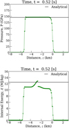 |
Fig. 5 Snap shots of the pressure and internal energy. Here we show the pressure (a) and internal energy (b) with vertical distance z at time t of 0.52 s for one-dimensional propagation of a shock wave produced by an impact simulation with a velocity of υimp = 10 km s−1 for a static basaltic cylindrical body at z ≤ 0 vertically colliding with another moving body at z = 0 at t = 0. Each green line shows simulation results and black lines correspond to the analytical solutions given by the Hugoniot relation. For z ≈ −6–0 km, the pressure and internal energy are increased by the shock wave, which should agree with the analytic solutions. |
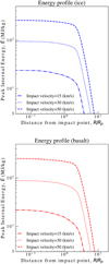 |
Fig. 6 Peak internal energy profile. We convert shock internal-energy according to the Hugoniot curve (E = E(P)). |
3.4 Difference between pressure and internal energy
Figure 6 shows the shock field of the revised internal energy. Its radial profiles are similar to those of the pressure (Fig. 3). The values of pressure and internal energy are almost independent of distance for R ≲ Rv, while they decrease with R for R ≳ Rv. The radial decay for R ≳ Rv is approximated as a power-law function of R. The power-law exponent at R >> Rv is approximated to −3 for the internal energy, while that for the pressure tends to be larger than that for the internal energy. We analytically investigate the shock pressure field in Sect. 4.
4 Analytical expression for the shocked state
4.1 Thermal term versus cold term
As mentioned in Sect. 2.1, the ANEOS model provides thermodynamic quantities from the Helmholtz free energy F. According to Eq. (2), the pressure P and internal energy E are given as:
 (4a)
(4a)
 (4b)
(4b)
where Et = Ft + TS and Ec = Fc, and S is the entropy calculated from F as S = −(∂F/∂T)ρ. The pressure and internal energy are composed of the thermal and cold terms, shown in Eqs. (4a) and (4b).
In Fig. 7, we plot Pt, Pc, Et, and Ec according to the Hugoniot curves as a function of ρ. In Fig. 7, the cold-term pressure, Pc, is dominant for ρ/ρ0 ≲ 2 – 4, while the thermal-term mainly governs the internal energy even for low density. Therefore, the internal energy is mainly determined by the thermal term.
We focus on the thermal term to derive the shocked internal energy. According to Melosh (2007), the definition of Ft in the ANEOS model is given by
![Mathematical equation: $\eqalign{ & {F_{\rm{t}}}(\rho ,T) \cr & = N{k_{\rm{B}}}T\left[ {3\ln (1 - {{\rm{e}}^{ - {T_{\rm{D}}}/T}}) - D\left( {{{{T_{\rm{D}}}} \over T}} \right) + {3 \over 2}{{\ln (1 + {\psi ^b})} \over b}} \right], \cr} $](/articles/aa/full_html/2024/08/aa50177-24/aa50177-24-eq8.png) (5)
(5)
where N is the total number of atoms per unit mass, kB is the Boltzmann constant, the constant b is a convergence parameter (0 < b ≤ 1), TD is the Debye temperature and D is a Debye function, defined as:
 (6)
(6)
and ψ is the dimensionless function, defined as:
 (7)
(7)
where C13 is a constant parameter. Based on Eqs. (4a) and (4b), the thermal terms for pressure and internal energy are written as:
 (8a)
(8a)
 (8b)
(8b)
According to Eqs. (8a) and (8b), Pt and Et are characterized by the Debye temperature, TD.
Behind the strong shock wave with which we are concerned, the temperature is much higher than the Debye temperature. We investigate the dependence of S on T for T >> TD, where
![Mathematical equation: $\eqalign{ & {\rm{S}} = {P_{\rm{t}}}{(2\rho {E_{\rm{t}}})^{ - 1}} + 1 \cr & \,\,\, = {1 \over {3(1 + {\psi ^{ - b}})}}{[D({T_{\rm{D}}}/T) - (1 + {\psi ^{ - b}})/2]^{ - 1}}. \cr} $](/articles/aa/full_html/2024/08/aa50177-24/aa50177-24-eq13.png) (9)
(9)
Figure 8 shows 𝒮 on the Hugoniot curve for water ice and basalt as a function of temperature. As shown in Fig. 8, 𝒮 is a constant value dependent on materials. Therefore, the relation between Pt and Et for T >> TD is approximately given by
 (10)
(10)
where 𝒮 = 1.26 and 1.4 for water ice and basalt, respectively. In Eq. (10), S can be connected with a Grüneisen parameter Γ for an ideal gas by 𝒮 = (1 + Γ)/2. In the following section, we show the derivation of the analytical solution for the shock internal energy based on the EoS (Eq. (10)).
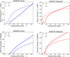 |
Fig. 7 Thermal and cold terms in the pressure and the internal energy for ice and basalt. Each dashed line expresses the cold term and is simply calculated by Pc = P(p) and Ec = E(p), and then solid lines are derived by subtracting the cold term from the Hugoniot curve, including the thermal pressure as well. Horizontal values are scaled by the reference density of each material. |
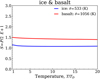 |
Fig. 8 Dependence of S on temperature. 𝒮 = Pt/2ρEt + 1 based on the ANEOS Hugoniot curve for water ice (blue) and basalt (red) as a function of the temperature scaled by the Debye temperatures TD. |
4.2 Analytical solution for the shock internal energy
4.2.1 Isobar¡c core
The particle velocity uv at the isobaric core is obtained from the impedance matching method (Melosh 1989). For impact between bodies of the same material, the impedance matching gives
 (11)
(11)
where υimp is the impact velocity. Here, we assume E ≈ Et, P ≈ Pt ,T ≈ TD and Eq. (10) gives the EoS as
 (12)
(12)
Using Eq. (12) and Eqs. (3a)–(3c) with P0 << P and E0 << E, we then have
 (13)
(13)
 (14)
(14)
 (15)
(15)
 (16)
(16)
We have P and E at the isobaric core, using Eqs. (15) and (16) coupled with Eq. (11).
The solutions for P and E, Eqs. (15) and (16), are consistent with a one-dimensional shock-tube solution, if high-velocity collisions result in E ≈ Et and P ≈ Pt. In Fig. 5, we show the result of the one dimensional problem for basalt with 10 km s−1. Equations (15), (16), and (11) give P = 1.02 × 10² GPa and E = 12.5 MJ kg−1. The solution for E agrees well with the simulation result, while P given by Eq. (15) is underestimated. This is mainly caused by the considerable value of Pc. Therefore, the assumption of Eq. (12) is valid for deriving E, while the additional modification is necessary to compensate for the underestimate of P.
We also investigate the dependence of shock fields on the projectile shapes (Fig. 9). For cylinders, E obtained from the simulations is in good agreement with that given by Eq. (16). For spherical bodies, E obtained from the simulations is slightly smaller than Eq. (16), because the one dimensional assumption is not so valid. However, the difference is minor.
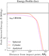 |
Fig. 9 Shock internal-energy field for spheroid and cylinder projectiles with υimp 30 km s−1. For the projectiles, their radii and height Rp are 500 m. We note that the cylinder projectile with a slab target differs from the collision between cylinders in Fig. 5. The black line is given in Eq. (16) with Eq. (11). |
4.2.2 Decay region
We focus on the region distant from the impact point. The shock field for E and P decays as a function of distance, in a similar way to a blast wave induced by a strong explosion. For spherical symmetry, a self-similar solution determines the shock field. Therefore, the dimensionless length ξ then gives the solutions (e.g., Landau & Lifshitz 1959), where
 (17)
(17)
Here Rc is the distance from the center of the isobaric core, whereas the distance is measured from the explosion point in the blast wave problem, and 𝒦imp is the impact kinetic energy. Projectiles are much smaller than targets, and therefore
 (18)
(18)
where Rp is the radius of the projectile.
The peak values for E and P are achieved behind the shock wave location Rs. The shock wave velocity Vs is given by
 (19)
(19)
where
 (20)
(20)
Here we assume the EoS given in Eq. (12). Using the Hugoniot curve given in Eqs. (13)–(16) with Eqs. (18) and (19), we have the peak pressure and internal energy with Rc instead of Rs:
 (21)
(21)
 (22)
(22)
To obtain the constant ξs, we use the energy conservation. We consider that the initial thermal energy of colliding bodies is much smaller than the impact energy, 𝒦imp. The total energy of the inner region of the target material bounded by the shock wave then corresponds to 𝒦imp:
 (23)
(23)
Equation (23) can be rewritten as
 (24)
(24)
where G, V, and Z are functions of χ, as given in Appendix. A. Therefore, ξs is given by Eq. (24) with Eqs. (A.5)–(A.12), and then ξs = 1.09 and 1.19 for ice (𝒮 = 1.26) and basalt (𝒮 = 1.4), respectively.
We assume that the internal energy is given by the harmonic mean of the shock internal energies in the isobaric core Ecore (Eq. (16)) and the decay region Edecay (Eq. (22)).
 (25)
(25)
where R0 is set at the center of the isobaric core. To apply Edecay given in Eq. (22), we set Rc = R − R0 and R0 = 1.8 Rp for ice and basalt, respectively. Although the solution depends on materials  (see Eq. (22)), the values of 𝒮 and ξs are similar, namely (𝒮,ξs) = (1.26, 1.09) and (1.4, 1.19) for ice and basalt, respectively. Therefore the solution is almost independent of the type of material.
We show the solutions for each material as dotted lines in Fig. 10 and compare them with simulation results. Figure 10 corresponds to the shock internal-energy field for impacts between icy or basalt bodies with 30 km s−1. Because of the similarity between the values of ξs and S, the solutions for the two different materials mostly reproduce the same value. Also, the solutions are mostly consistent with the simulations at R ≲ 2Rp as discussed in Sect. 4.2.1.
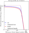 |
Fig. 10 Shock internal-energy field for ice (blue) and basalt (red) bodies with υimp=30 km s−1. Solid curves are the results of simulations. Dotted lines are the analytic solution given by Eq. (25) with R0 = 1.8RP. For reference, the black arrow is the isobaric-core solution in Eq. (16) with Eq. (11), which is independent of the type of the material. |
4.3 Analytical solution for shock pressure
As shown in Sects. 4.2.1 and 4.2.2, the internal energy is reproduced by the analytic solution with the EoS of Eq. (12). However, the analytic solution underestimates the pressure for P ≲ 20 GPa (ice) and 300 GPa (basalt). This is caused by the importance of Pc for low pressure (see Fig. 7). Therefore, the additional modification is needed to compensate for this underestimation.
We consider E –as derived in Eqs. (16) and (22) – to be accurate. We then recalculate the density ρ* corresponding to E from the Hugoniot curve given by ANEOS (see lower two panels in Fig. 7). We obtain P* corresponding to ρ* from the Hugoniot curve (upper two panels in Fig. 7). The shock pressure is thus given by P*.
Figure 11 shows the pressures at isobaric cores as a function of impact velocity. Equation (15) is in good agreement with the simulation results for the high velocity, while Eq. (15) underestimates for low-velocity region. The modified pressure P* reproduces the simulation results even for low velocities.
The agreement between the analytical solution and simulation result for E and P* indicates the validity of the assumption. The shock wave is mainly driven by the thermal terms. The internal energy is accurately estimated from the simple EoS of Eq. (12). The pressure and density are determined by the internal energy induced by a shock wave, and are obtained from the values corresponding to the internal energy according to the Hugoniot curve.
According to the analytic solution for the internal energy, we assume that the pressure is given by the harmonic mean of  .
.
 (26)
(26)
where  are the analytic solution for the isobaric core and the decay region, respectively, and the setting of R0 is the same as the internal energy. Figure 12 shows the shock pressure fields obtained from simulations and the analytical solution for icy and basaltic bodies with υimp = 30 km s−1. The analytical solution P* reproduces the shock pressure field from the isobaric core to the decay region.
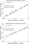 |
Fig. 11 Comparison between analytical solutions and simulation results. The peak pressures of these plots are recorded in the nearest tracer particle to the impact point. The shape and color of the markers in the plots correspond to projectile shape: cylinder (green square) and spheroid (black circle). The simulation with the cylinder projectile is the same as that shown in Fig. 9. Solid lines are illustrated by Eq. (15) and P* (Sect. 4.3). |
5 Angle dependence
The previous section focus on the vertical shock fields in previous sections. In this section, we discuss the shock fields along other directions and investigate the dependence of shock pressure fields on the angles from the impact point.
Figure 13 shows the shock pressure fields with υimp = 30 km s−1. We note that the horizontal value Rc is not the distance from the impact point R, but the distance from the center of the core. We set the center of core at z = −1.8 Rp, which is same as R0(see Sect. 4.2.2). It should be noted that the angle θ is measured from the vertical direction; that is θ = 0 is for the vertical shock fields. As shown in Fig. 13, the pressure fields are almost independent of θ ≲ 60°, while the angle dependence is strong for θ ≳ 60°. The interference between rarefaction and shock waves may modify the pressure field especially for θ ≳ 90°. In addition, for large angles θ ≳ 60°, the shock wave propagation deviates from the isotropic expansion from the core assumed for our analysis. However, the relative difference between pressures from the analytical solution and the numerical result at Rc = 3 Rv is within 30% if θ ≤ 60° for both materials, but is within 10% for basalt (Fig. 13).
In Sect. 4.2.2, our solutions based on the assumption of spherical symmetry are valid for the shock fields orientated in the vertical direction θ = 0°. Figure 13 shows that our assumption of the spherical symmetry is valid for the shock fields with small angles, such as 0 ≤ θ ≤ 60° for ice and basalt.
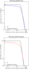 |
Fig. 12 Shock pressure fields in an impact event with impact velocity υimp = 30 km s−1 for ice (a) and basalt (b) obtained from iSALE simulations (long-dashed lines) and from the analytical solution (solid lines). For reference, the black arrow indicates the analytic solution in the iso-baric core. |
6 Atmosphere formation: Impact vaporization
6.1 The amount of vapor due to an impact
The shock wave in impact events can generate an extremely high temperature field, and so this event may shape planetary atmospheres. The accretion process contributes to the growth of terrestrial atmospheres (e.g., Benlow & Meadows 1977; Lange & Ahrens 1982). The amount of vapor production is derived from the shocked state because the subsequent process leading to shock compression can be assumed as the isentropic expansion (Sugita & Schultz 2002); therefore, the shock entropy field determines the amount of vapor (Ahrens & O’keefe 1977). For that reason, the isentropic expansion after the shock compression is illustrated by the vertical line from a point on the Hugoniot curve to the horizontal direction in Fig. 14. The final pressure during isentropic expansion depends on the ambient pressure. In Fig. 15, we set the final pressure PF at the triple point pressure of H2O, PF = 611 Pa, which is the same as in Kraus et al. (2011). For material that reaches the intermediate regions between liquid and vapor, the mass of the partial vapor is given by the lever arm rule (e.g., Kraus et al. 2011).
Our analytic solutions allow us to obtain the entropy field using the ANEOS Hugoniot relation, S = S(E). From this, we can derive the amount of vapor as a function of impact velocity (Fig. 15).
The analytic solutions reproduce the consistent value with simulation results (Fig. 15). The analytical solution overestimates the amount of vapor compared to simulation results for basaltic bodies with low impact velocities of υimp ≲ 20 km s−1, for which vaporization mainly occurs in isobaric cores. Although our analytic solution accurately represents the peak pressure in the isobaric core (Fig. 11), the shock pressure in the core slightly decreases with distance (Fig. 12). Our analytic solution ignores this slight decline in the isobaric core, and gives the amount of vapor according to the isobaric-core solution. The slight overestimation around the edges of isobaric cores leads to the overestimation in the amounts of vapors for basalt bodies with low velocities υimp ≲ 20 km s−1 (Fig. 15). However, our analytic solution is useful for estimating the amount of impact vapor. Figure 16 illustrates our analytical estimation of the amount of vapor for an impact on a basaltic planet with an ambient pressure of PF. The amount of vapor is the increase function of impact velocity. If impact velocities are higher than 20 km s−1, the dependence on PF is small.
It should be noted that we obtain the amount of vapor under the assumption of fluid dynamics. Other heating effects, such as shear heating, may influence the shocked state especially below υimp ≲ 12 km s−1 (Manske et al. 2022). However, our analytical solution is in good agreement with the numerical results for the high-speed impact region at υimp ≳ 25 km s−1, with the relative error between the two results being less than 60%.
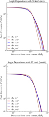 |
Fig. 13 Dependence of shock pressure on the angle of the shock field to the vertical direction. The figure shows shock pressure fields for ice and basalt bodies as a function of the distance from the center of isobaric core Rc (Sect. 4.2.2). Each color corresponds to a different angle measured from the core center and θ = 0° is defined as the vertical direction. |
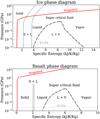 |
Fig. 14 Phase diagram for water ice and basalt from the ANEOS (Turtle & Pierazzo 2001; Pierazzo et al. 2005) with the Hugoniot curves (red line). The dotted line and dash-dotted lines correspond to the phase boundary for solid-liquid and liquid-vapor, respectively. |
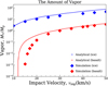 |
Fig. 15 Scaled mass of water ice and basalt that have been vaporized. These plots represent simulation results and lines are given by our solutions. The mass of vapor MV includes both the mass of the target and the projectile. |
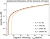 |
Fig. 16 Analytical estimation of the mass of the vapor production of basaltic bodies for target and projectile materials, scaled by the projectile mass. Each color corresponds to different final pressure PF. |
6.2 Reformation of planetary atmospheres during accretion process in a giant impact
In the final formation stage of the terrestrial planets of the Solar System, mars-sized protoplanets formed and terrestrial planets then formed via collisions between these protoplanets, called giant impacts, which were induced by the long-term chaotic orbital instability (e.g., Chambers & Wetherill 1998).
In a giant-impact event, the planetary bodies receive violent impact energies, and then eject some of their material (e.g., Shuvalov et al. 2014; Stewart et al. 2014; Kurosaki & Inutsuka 2023). The planetary atmospheres are easily removed by the impact event (Kurosaki & Inutsuka 2023). On the other hand, the secondary accretion of solid giant-impact ejecta may cause reformation of the atmospheres. In this section, we estimate the formation of the atmospheres through the accretion process.
A giant impact ejects a certain amount of small bodies, which amount to approximately 10% of the mass of the colliding pro-toplanets (Genda et al. 2015). The ejecta from a giant impact finally distribute as a disk around the host star. The total mass of the giant-impact ejecta mainly decreases due to the colli-sional cascade among the giant-impact ejecta with the blow-out of micron-sized or smaller bodies (Kobayashi et al. 2019). However, some of the giant-impact ejecta are accreted onto the parent planet.
Considering a basaltic planet with mass Mplanet around a host star of solar mass, the relative velocity υrel between the planet and the ejecta is roughly given by 1–3υesc, where υesc is the escape velocity of the planet (Genda et al. 2015). Here we set to  . The accretion timescale for the reduction of the giant-impact ejecta is estimated as
 (27)
(27)
where a is the semimajor axis of the planet, ρ is the solid density of the planet and the ejecta, and M⊙ is the Earth mass.
On the other hand, the timescale of the collisional cascade is characterized by the mass of largest ejecta mc, which is estimated to (Kobayashi & Tanaka 2010; Kobayashi et al. 2019),
 (28)
(28)
where Mej is the total mass of the giant-impact ejecta.
For a giant impact of protoplanets, Mej is typically given by ∽0.1 Mplanet. For Mplanet = M⊕, a giant impact gives Mej ≈ 0.1 M⊕, resulting in τcc << τacc (compare between Eqs. (27) and (28)). The giant-impact ejecta mass Mej thus decreases via the collisional cascade. Once Mej ≲ 10−5M⊕, τcc is longer than τacc. The giant-impact ejecta are then mainly accreted onto the planet. Therefore, the accretion mass of giant-impact ejecta Mej,ac is estimated from τacc = τcc as,
 (29)
(29)
Interestingly Mej,ac is independent of a, because the dependence of τacc and τcc on a is the same. Mej,ac is larger for larger mc. The accretion mass Mej,ac decreases with Mplanet.
Using Mej,ac with the impact velocity given by  , we calculate the atmosphere mass Matm composed of vapor caused by the impacts with the giant-impact ejecta for PF = 105 Pa (see Fig. 17). Again, we note that the choice of PF is unimportant here (see Fig. 16). For Mplanet = M⊕, υimp ≈ 22 km s−1, resulting in Matm ≈ 0.3Mej,ac. As shown in Fig. 17, the atmospheric mass of Earth is reproduced by impact vaporization with mc ≳ 1021 g, while Venus’s atmosphere needs mc ≳ 1024 g. While the accretion mass Mej,ac decreases with Mplanet (Eq. (29)), the vapor mass significantly depends on υimp (Fig. 16) and thus Matm increases with Mplanet because of the dependence of υimp on Mplanet. Post-impact atmospheres become composed of H2O and CO2 via chemical evolution on a timescale of 106 yr (Lupu et al. 2014). The substantial evolution mainly reduces the atmosphere mass. The giant-impact ejecta with mc ≳ 1024 g are likely to reproduce planetary atmospheres in the Solar System.
We note that mc depends on the collisional parameters of giant impacts. According to collisional simulations with colli-sional parameters given by N-body simulations for giant-impact stages, typical giant impacts result in mc ≳ 1024 g (Genda et al. 2015). In addition, planets resulting from N-body simulations have highly eccentric orbits, which are inconsistent with the present orbits of Earth and Venus. The dynamical friction with giant-impact ejecta is possible to decay the eccentricities. This decay requires τcc, which is longer than the timescale of the dynamical friction, which means mc ≳ 1024 g (Kobayashi et al. 2019). The terrestrial planets in the Solar System may be formed from giant impacts with mc ≳ 1024 g. On the other hand, if giant impacts result in smaller mc, the resultant planets may have high eccentricities and small Matm. Therefore, our scenario implies that Matm has the correlation with orbital eccentricities.
Above, we discuss the formation of secondary atmospheres subsequent to a giant impact. A primary atmosphere is obtained from a protoplanetary disk and is mainly composed of H2 and He. On the other hand, the composition of the secondary atmosphere due to impacts is similar to that of atmospheres formed by reactions between a primary atmosphere and a magma ocean (e.g., Itcovitz et al. 2022; Kurosaki et al. 2023). The primary atmosphere evolution may produce H2O without experiencing a giant impact (e.g., Ikoma & Genda 2006; Kimura & Ikoma 2022). If a planet has an ocean, the surface ocean may influence the heating process and atmosphere stripping (e.g., Genda & Abe 2005; Schlichting et al. 2015; Lock & Stewart 2024). Even in such complicated situations, our analytical formula may be applied to calculate the amount of vapor using the 𝒮 value for oceans. However, the chemical reactions between vapors from rocky body and ocean should be considered in the subsequent evolution, and these will be addressed in a future study.
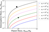 |
Fig. 17 Atmosphere mass Matm produced by the accretion process following a giant impact, as a function of the planetary mass Mplanet. Each color corresponds to the mass of the largest ejecta mc. The circle and diamond represent the atmospheric masses of Earth and Venus, respectively. |
7 Summary
A high-speed planetary impact causes a shock wave, which is expected to occur in the late stages of planet formation. Then, the shock wave can form an extremely high-pressure field called the shock pressure field. We have investigated the structure of the shock pressure field in impact simulations with iSALE-2D using ANEOS, which is one of the most sophisticated EoS models. We have obtained two specific features of the shock field as a function of distance, the isobaric core around the impact point and the decay region distant from the impact point (Sect. 3.2). To understand the shock fields, we have investigated the contribution of the thermal and cold terms in the solid EoS model on the Hugoniot curves. We find that the shock pressure field is determined by both the thermal and cold terms, while the cold term makes a minor contribution to the shock internal-energy field.
We have thus used a simple EoS based only on the thermal term. To obtain analytical solutions for the shock internal-energy field, we assume the shock wave as a strong explosion with spherical symmetry. Under this assumption, we have derived analytical solutions for the shock internal-energy field (Sect. 4.2). Furthermore, we have additionally given analytical solutions for the shock pressure using the Hugoniot curve (Sect. 4.3). These solutions based on the spherical symmetry are valid to vertical direction along the impact direction.
To investigate the applicability of our solutions to other directions, we have analyzed the shock pressure field in various directions. We have found that as the angle from the vertical axis increases, the errors on the shock pressure from the vertical direction became large. However, as discussed in Sect. 5, our assumption of spherical symmetry is valid for θ ≤ 60°. The angle should be measured from the center of the core set properly.
Using our solutions for the shock field, we show the amount of vapor production due to an impact event (Sect. 6.1). We also estimate the planetary atmosphere mass formed by the accretion of ejecta from a giant impact (Sect. 6.2). Our findings can explain the amounts of planetary atmosphere found on the terrestrial planets of the Solar System.
Acknowledgements
We are grateful to the anonymous referee for beneficial comments. We thank iSALE developers, including G. Collins, K. Wünnemann, B. Ivanov, J. Melosh, and D. Elbeshausen. We used pySALEplot to analyze the result of iSALE and to make figures. We thank Tom Davison for the development of pySALEplot. Our numerical simulations were carried out on the general-purpose PC cluster at Center for Computational Astrophysics. I would like to take this opportunity to thank the “Interdisciplinary Frontier Next-Generation Researcher Program of the Tokai Higher Education and Research System”. The work is supported by Grants-in-Aid for Scientific Research (21K03642, 22H01278, 22H00179) from MEXT of Japan.
Appendix A Derivation of ξs
The assumption of a strong explosion with spherical symmetry allows to write the integrand in Eq. (23) with dimensionless functions of ξ as
 (A.1)
(A.1)
 (A.2)
(A.2)
 (A.3)
(A.3)
 (A.4)
(A.4)
The functions V, G, and Z are given by solving fluid equations with boundary conditions at ξ = ξs (Landau & Lifshitz 1959).
![Mathematical equation: $\eqalign{ & {\left[ {{{2(3S - 2)V - 5} \over {(S - 4)/S}}} \right]^a}{\left[ {{{(2S - 1)V - 1} \over {(S - 1)/S}}} \right]^b} \cr & & & & \times {(SV)^{ - 2/5}} = \chi , \cr} $](/articles/aa/full_html/2024/08/aa50177-24/aa50177-24-eq43.png) (A.5)
(A.5)
![Mathematical equation: $\eqalign{ & G = {{\cal S} \over {{\cal S} - 1}}{\left[ {{{2(3{\cal S} - 2)V - 5} \over {({\cal S} - 4)/{\cal S}}}} \right]^{{a^\prime }}} \cr & \,\,\,\, \times {\left[ {{{(2{\cal S} - 1)V - 1} \over {(S - 1)/{\cal S}}}} \right]^{{b^\prime }}}{\left[ {{{V - 1} \over {(1 - {\cal S})/{\cal S}}}} \right]^{{c^\prime }}}, \cr} $](/articles/aa/full_html/2024/08/aa50177-24/aa50177-24-eq44.png) (A.6)
(A.6)
 (A.7)
(A.7)
where χ = ξ/ξs and
 (A.8)
(A.8)
 (A.9)
(A.9)
 (A.10)
 (A.11)
 (A.12)
Substituting Eqs. (A.1)–(A.4) into Eq. (23), we have Eq. (24). For the integration in Eq. (24), V, G, and Z are obtained as functions of χ, using Eqs. (A.6)–(A.7).
References
- Ahrens, T. J., & O’Keefe, J. D. 1972, Moon, 4, 214 [NASA ADS] [CrossRef] [Google Scholar]
- Ahrens, T. J., & O’keefe, J. D. 1977, in Impact and Explosion Cratering: Planetary and Terrestrial Implications, eds. D. J. Roddy, R. O. Pepin, & R. B. Merrill, 639 [Google Scholar]
- Amsden, A. A., Ruppel, H. M., & Hirt, C. W. 1980, SALE: a simplified ALE computer program for fluid flow at all speeds, los Alamos National Laboratory Report LA-8095 [CrossRef] [Google Scholar]
- Benlow, A., & Meadows, A. J. 1977, Ap&SS, 46, 293 [NASA ADS] [CrossRef] [Google Scholar]
- Bowling, T. J., Johnson, B. C., Wiggins, S. E., et al. 2020, Icarus, 343, 113689 [NASA ADS] [CrossRef] [Google Scholar]
- Chambers, J. E., & Wetherill, G. W. 1998, Icarus, 136, 304 [NASA ADS] [CrossRef] [Google Scholar]
- Croft, S. K. 1982, Geol. Soc. Am. Spec. Pap., 190, 143 [Google Scholar]
- Genda, H., & Abe, Y. 2005, Nature, 433, 842 [NASA ADS] [CrossRef] [Google Scholar]
- Genda, H., Fujita, T., Kobayashi, H., Tanaka, H., & Abe, Y. 2015, Icarus, 262, 58 [NASA ADS] [CrossRef] [Google Scholar]
- Ikoma, M., & Genda, H. 2006, ApJ, 648, 696 [NASA ADS] [CrossRef] [Google Scholar]
- Itcovitz, J. P., Rae, A. S. P., Citron, R. I., et al. 2022, PSJ, 3, 115 [Google Scholar]
- Ivanov, B., Deniem, D., & Neukum, G. 1997, Int. J. Impact Eng., 20, 411 [NASA ADS] [CrossRef] [Google Scholar]
- Kadono, T., Sugita, S., Mitani, N. K., et al. 2002, Geophys. Res. Lett., 29, 1979 [Google Scholar]
- Kimura, T., & Ikoma, M. 2022, Nat. Astron., 6, 1296 [NASA ADS] [CrossRef] [Google Scholar]
- Kobayashi, H., & Tanaka, H. 2010, Icarus, 206, 735 [NASA ADS] [CrossRef] [Google Scholar]
- Kobayashi, H., Tanaka, H., Krivov, A. V., & Inaba, S. 2010, Icarus, 209, 836 [CrossRef] [Google Scholar]
- Kobayashi, H., Tanaka, H., & Krivov, A. V. 2011, ApJ, 738, 35 [NASA ADS] [CrossRef] [Google Scholar]
- Kobayashi, H., Isoya, K., & Sato, Y. 2019, ApJ, 887, 226 [NASA ADS] [CrossRef] [Google Scholar]
- Kurosaki, K., & Inutsuka, S.-i. 2023, ApJ, 954, 196 [NASA ADS] [CrossRef] [Google Scholar]
- Kraus, R. G., Senft, L. E., & Stewart, S. T. 2011, Icarus, 214, 724 [NASA ADS] [CrossRef] [Google Scholar]
- Kraus, R. G., Root, S., Lemke, R. W., et al. 2015, Nat. Geosci., 8, 269 [NASA ADS] [CrossRef] [Google Scholar]
- Kurosaki, K., Hori, Y., Ogihara, M., & Kunitomo, M. 2023, ApJ, 957, 67 [NASA ADS] [CrossRef] [Google Scholar]
- Landau, L. D., & Lifshitz, E. M. 1959, in Fluid Mechanics (Oxford: Pergamon Press) [Google Scholar]
- Lange, M. A., & Ahrens, T. J. 1982, Icarus, 51, 96 [NASA ADS] [CrossRef] [Google Scholar]
- Lock, S. J., & Stewart, S. T. 2024, Planet. Sci. J., 5, 28 [NASA ADS] [CrossRef] [Google Scholar]
- Lupu, R. E., Zahnle, K., Marley, M. S., et al. 2014, ApJ, 784, 27 [NASA ADS] [CrossRef] [Google Scholar]
- Manske, L., Wünnemann, K., & Kurosawa, K. 2022, J. Geophys. Res. (Planets), 127, e2022JE007426 [NASA ADS] [CrossRef] [Google Scholar]
- Melosh, H. J. 1989, Impact Cratering: A Geologic Process (Oxford: Oxford University Press) [Google Scholar]
- Melosh, H. J. 2007, M&PS, 42, 2079 [NASA ADS] [Google Scholar]
- Melosh, H. J., & Vickery, A. M. 1989, Nature, 338, 487 [NASA ADS] [CrossRef] [Google Scholar]
- Mizutani, H., Takagi, Y., & Kawakami, S.-I. 1990, Icarus, 87, 307 [NASA ADS] [CrossRef] [Google Scholar]
- Monteux, J., & Arkani-Hamed, J. 2016, Icarus, 264, 246 [NASA ADS] [CrossRef] [Google Scholar]
- Monteux, J., & Arkani-Hamed, J. 2019, Icarus, 331, 238 [NASA ADS] [CrossRef] [Google Scholar]
- Pierazzo, E., & Melosh, H. J. 2000, Icarus, 145, 252 [NASA ADS] [CrossRef] [Google Scholar]
- Pierazzo, E., Vickery, A. M., & Melosh, H. J. 1995, in Lunar and Planetary Science Conference, 26, Lunar and Planetary Science Conference, 1119 [NASA ADS] [Google Scholar]
- Pierazzo, E., Vickery, A. M., & Melosh, H. J. 1997, Icarus, 127, 408 [NASA ADS] [CrossRef] [Google Scholar]
- Pierazzo, E., Artemieva, N., & Ivanov, B. 2005, in Large Meteorite Impacts III (Geological Society of America) [Google Scholar]
- Schlichting, H. E., Sari, R., & Yalinewich, A. 2015, Icarus, 247, 81 [NASA ADS] [CrossRef] [Google Scholar]
- Shuvalov, V., Kührt, E., de Niem, D., & Wünnemann, K. 2014, Planet. Space Sci., 98, 120 [Google Scholar]
- Stewart, S. T., Seifter, A., & Obst, A. W. 2008, Geophys. Res. Lett., 35, L23203 [NASA ADS] [CrossRef] [Google Scholar]
- Stewart, S. T., Lock, S. J., & Mukhopadhyay, S. 2014, in 45th Annual Lunar and Planetary Science Conference, Lunar and Planetary Science Conference, 2869 [Google Scholar]
- Suetsugu, R., Tanaka, H., Kobayashi, H., & Genda, H. 2018, Icarus, 314, 121 [NASA ADS] [CrossRef] [Google Scholar]
- Sugita, S., & Schultz, P. H. 2002, Icarus, 155, 265 [NASA ADS] [CrossRef] [Google Scholar]
- Thompson, S. L., & Lauson, H. S. 1972, Improvements in the Chart D Radiation-Hydrodynamic Code. III: Revised Analytic Equations of State, Albuquerque, New Mexico: Sandia National Laboratory, Technical Report SC-RR-71-0714 [Google Scholar]
- Thompson, S. L., Lauson, H. S., Melosh, H. J., Collins, G. S., & Stewart, S. T. 2019, M-ANEOS [Google Scholar]
- Tonks, W. B., & Melosh, H. J. 1993, JGR, 98, 5319 [NASA ADS] [CrossRef] [Google Scholar]
- Turtle, E. P., & Pierazzo, E. 2001, Science, 294, 1326 [CrossRef] [Google Scholar]
- Wünnemann, K., Collins, G. S., & Melosh, H. J. 2006, Icarus, 180, 514 [CrossRef] [Google Scholar]
All Figures
|
Fig. 1 Maximum pressure distribution caused by an impact, also called the shock pressure field, for basalt bodies with an impact speed of 30 km−1. The red curve is the result for 20 cppr, while the blue curve is for 50 cppr. |
| In the text | |
|
Fig. 2 Result of the iSALE simulation. The changes to pressure and the internal energy caused by an impact shock with υimp = 30 km s−1 are illustrated as a function of position at t = 0 (a), t = ts (b), and t = 4ts (c). Calculation time is scaled by the time ts, where ts = 2Rp/υimp. |
| In the text | |
|
Fig. 3 Peak pressure profile formed by the shock compression as a function of distance from the impact point along the vertical axis. The distance is characterized by projectile radius Rp. We note that the vertical value, peak pressure, is not a pressure at each time but the maximum pressure reached at each point. Tracer particles along with a white arrow (Fig. 2) record maximum pressure as a function of initial position, and these values are shown here. |
| In the text | |
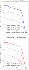 |
Fig. 4 Same as Fig. 3, but for internal energy instead of pressure. |
| In the text | |
|
Fig. 5 Snap shots of the pressure and internal energy. Here we show the pressure (a) and internal energy (b) with vertical distance z at time t of 0.52 s for one-dimensional propagation of a shock wave produced by an impact simulation with a velocity of υimp = 10 km s−1 for a static basaltic cylindrical body at z ≤ 0 vertically colliding with another moving body at z = 0 at t = 0. Each green line shows simulation results and black lines correspond to the analytical solutions given by the Hugoniot relation. For z ≈ −6–0 km, the pressure and internal energy are increased by the shock wave, which should agree with the analytic solutions. |
| In the text | |
|
Fig. 6 Peak internal energy profile. We convert shock internal-energy according to the Hugoniot curve (E = E(P)). |
| In the text | |
|
Fig. 7 Thermal and cold terms in the pressure and the internal energy for ice and basalt. Each dashed line expresses the cold term and is simply calculated by Pc = P(p) and Ec = E(p), and then solid lines are derived by subtracting the cold term from the Hugoniot curve, including the thermal pressure as well. Horizontal values are scaled by the reference density of each material. |
| In the text | |
|
Fig. 8 Dependence of S on temperature. 𝒮 = Pt/2ρEt + 1 based on the ANEOS Hugoniot curve for water ice (blue) and basalt (red) as a function of the temperature scaled by the Debye temperatures TD. |
| In the text | |
|
Fig. 9 Shock internal-energy field for spheroid and cylinder projectiles with υimp 30 km s−1. For the projectiles, their radii and height Rp are 500 m. We note that the cylinder projectile with a slab target differs from the collision between cylinders in Fig. 5. The black line is given in Eq. (16) with Eq. (11). |
| In the text | |
|
Fig. 10 Shock internal-energy field for ice (blue) and basalt (red) bodies with υimp=30 km s−1. Solid curves are the results of simulations. Dotted lines are the analytic solution given by Eq. (25) with R0 = 1.8RP. For reference, the black arrow is the isobaric-core solution in Eq. (16) with Eq. (11), which is independent of the type of the material. |
| In the text | |
|
Fig. 11 Comparison between analytical solutions and simulation results. The peak pressures of these plots are recorded in the nearest tracer particle to the impact point. The shape and color of the markers in the plots correspond to projectile shape: cylinder (green square) and spheroid (black circle). The simulation with the cylinder projectile is the same as that shown in Fig. 9. Solid lines are illustrated by Eq. (15) and P* (Sect. 4.3). |
| In the text | |
|
Fig. 12 Shock pressure fields in an impact event with impact velocity υimp = 30 km s−1 for ice (a) and basalt (b) obtained from iSALE simulations (long-dashed lines) and from the analytical solution (solid lines). For reference, the black arrow indicates the analytic solution in the iso-baric core. |
| In the text | |
|
Fig. 13 Dependence of shock pressure on the angle of the shock field to the vertical direction. The figure shows shock pressure fields for ice and basalt bodies as a function of the distance from the center of isobaric core Rc (Sect. 4.2.2). Each color corresponds to a different angle measured from the core center and θ = 0° is defined as the vertical direction. |
| In the text | |
|
Fig. 14 Phase diagram for water ice and basalt from the ANEOS (Turtle & Pierazzo 2001; Pierazzo et al. 2005) with the Hugoniot curves (red line). The dotted line and dash-dotted lines correspond to the phase boundary for solid-liquid and liquid-vapor, respectively. |
| In the text | |
|
Fig. 15 Scaled mass of water ice and basalt that have been vaporized. These plots represent simulation results and lines are given by our solutions. The mass of vapor MV includes both the mass of the target and the projectile. |
| In the text | |
|
Fig. 16 Analytical estimation of the mass of the vapor production of basaltic bodies for target and projectile materials, scaled by the projectile mass. Each color corresponds to different final pressure PF. |
| In the text | |
|
Fig. 17 Atmosphere mass Matm produced by the accretion process following a giant impact, as a function of the planetary mass Mplanet. Each color corresponds to the mass of the largest ejecta mc. The circle and diamond represent the atmospheric masses of Earth and Venus, respectively. |
| In the text | |
Current usage metrics show cumulative count of Article Views (full-text article views including HTML views, PDF and ePub downloads, according to the available data) and Abstracts Views on Vision4Press platform.
Data correspond to usage on the plateform after 2015. The current usage metrics is available 48-96 hours after online publication and is updated daily on week days.
Initial download of the metrics may take a while.