| Issue |
A&A
Volume 642, October 2020
|
|
|---|---|---|
| Article Number | A172 | |
| Number of page(s) | 29 | |
| Section | Stellar atmospheres | |
| DOI | https://doi.org/10.1051/0004-6361/202038464 | |
| Published online | 19 October 2020 | |
Atmospheric NLTE models for the spectroscopic analysis of blue stars with winds
V. Complete comoving frame transfer, and updated modeling of X-ray emission
1
LMU München, Universitätssternwarte,
Scheinerstr. 1,
81679
München,
Germany
e-mail: This email address is being protected from spambots. You need JavaScript enabled to view it.
2
Departamento de Astrofísica, Centro de Astrobiología (CSIC-INTA),
Ctra. Torrejón a Ajalvir km 4,
28850
Torreón de Ardoz,
Spain
3
KU Leuven, Instituut voor Sterrenkunde,
Celestijnenlaan 200D,
3001
Leuven,
Belgium
4
Argelander Institut für Astronomie der Universität Bonn,
Auf dem Hügel 71,
53121
Bonn,
Germany
Received:
22
May
2020
Accepted:
3
August
2020
Abstract
Context. Obtaining precise stellar and wind properties and abundance patterns of massive stars is crucial to understanding their nature and interactions with their environments, as well as to constrain their evolutionary paths and end-products.
Aims. To enable higher versatility and precision of the complete ultraviolet (UV) to optical range, we improve our high-performance, unified, NLTE atmosphere and spectrum synthesis code FASTWIND. Moreover, we aim to obtain an advanced description of X-ray emission from wind-embedded shocks, consistent with alternative modeling approaches.
Methods. We include a detailed comoving frame radiative transfer for the essential frequency range, but still apply methods that enable low turnaround times. We compare the results of our updated computations with those from the alternative code CMFGEN, and our previous FASTWIND version, for a representative model grid.
Results. In most cases, our new results agree excellently with those from CMFGEN, both regarding the total radiative acceleration, strategic optical lines, and the UV-range. Moderate differences concern He II λλ4200-4541 and N V λλ4603-4619. The agreement regarding N III λλ4634−4640−4642 has improved, though there are still certain discrepancies, mostly related to line overlap effects in the extreme ultraviolet, depending on abundances and micro-turbulence. In the UV range of our coolest models, we find differences in the predicted depression of the pseudo-continuum, which is most pronounced around Lyα. This depression is larger in CMFGEN, and related to different Fe IV atomic data. The comparison between our new and previous FASTWIND version reveals an almost perfect agreement, except again for N V λλ4603-4619. Using an improved, depth-dependent description for the filling factors of hot, X-ray emitting material, we confirm previous analytic scaling relations with our numerical models.
Conclusions. We warn against uncritically relying on transitions, which are strongly affected by direct or indirect line-overlap effects. The predicted UV-continuum depression for the coolest grid-models needs to be checked, both observationally, and regarding the underlying atomic data. Wind lines from “super-ionized” ions such as O VI can, in principle, be used to constrain the distribution of wind-embedded shocks. The new FASTWIND version v11 is now ready to be used.
Key words: methods: numerical / stars: atmospheres / stars: early-type / stars: massive / X-rays: stars
© ESO 2020
1 Introduction
The impact of massive stars on cosmic and galactic evolution (for example, Bresolin et al. 2008) has been widely appreciated within the astronomical community. In particular, the observational detection of merging black holes and neutron stars, via gravitational waves (Abbott et al. 2016, 2017), has renewed the interest in massive stellar objects, and especially in the evolution of (binary) black-hole progenitors (cf. Marchant et al. 2016; Langer et al. 2020; Petit et al. 2017). However, whether for single objects or objects in binary and multiple systems, current models of massive stars suffer from a number of uncertainties and simplified descriptions1, mostly related to the need for intrinsic multi-D processes to be “boiled down” to 1D. This is because of the much longer evolutionary timescales as compared to timescales governing the dynamics of specific processes. An important example is rotation (Langer et al. 1997; Maeder & Meynet 2000) and the induced mixing, which, moreover, is often treated by a simple diffusion approach, even if advective terms play an important role (exemplarily, for mixing due to meridional circulations, Maeder & Zahn 1998; Maeder & Meynet 2015).
In order to test these evolutionary models and related predictions on the one hand (for instance, regarding the surface composition, which strongly depends on rotational mixing, and, in binary systems, also on mass-overflow), and to calibrate various basically unknown coefficients (such as convective overshoot length, and mixing efficiencies) on the other, a careful comparison with observations (that is, with real objects) is inevitable.
Though “comparison with observations” sounds simple, it is not, since one does not “observe” temperatures, luminosities, mass-loss rates, rotational rates, surface abundances, etc., but rather infers them from the observed spectral energy distribution, often by applying a technique called “quantitative spectroscopy.” In brief, this procedure also adopts a simplified model, here for the outer, atmospheric layers of a star, and derives, on top of this model, the emitted photonic energy distribution.
Such synthetic spectra then depend on the specific combination of atmospheric parameters and chemical composition, and, by varying these quantities, one tries to simulate synthetic energy distributions that are as close as possible to the observed ones. The variation itself is obtained via comprehensive, pre-calculated model grids, or on the fly, for example when genetic algorithms are used to minimize the deviation between observed and synthetic spectra (Mokiem et al. 2005).
After an optimum fitting distribution has been found (for a large number of proven-to-work, diagnostic features, and spectral ranges), onethen claims to have derived (or even observed) the atmospheric parameters and surface abundances. Obviously, there is the immediate question of uniqueness (Can different combinations of parameters and abundances yield a similar agreement?), and the question about the influence of specific approximations and data on the final results.
Irrespective of these questions, it is clear that for such a procedure, a large number of theoretical spectra have to be synthesized, because the number of parameters describing an atmosphere is large, particularly for massive stars that displayline-radiation driven winds with densities that increase with stellar luminosity (reviewed by Puls et al. 2008).
Consequently, a prime factor for efficient spectral analyses is computational performance. Unfortunately, since massive stars are often hot and/or have a low-density atmosphere, the most time-saving assumption made for cooler stars with larger densities, namely thatthe atomic and ionic occupation numbers can be approximated from local thermodynamic equilibrium (LTE) conditions2 (but see, forexample, Bergemann et al. 2012), is no longer applicable. Instead, one needs to set up and solve the equations of statistical (sometimes also called kinetic) equilibrium, commonly denoted by non-LTE or NLTE. Such calculations are computationally expensive, since the radiation field, required to set up the radiative transition rates, and affected by velocity-field induced Doppler-shifts, needs to be computed at many frequency points, in an iterative approach. Moreover, NLTE requires the knowledge of numerous atomic and ionic properties of contributing species, such as cross-sections and collision strengths, which themselves can suffer from uncertainties of different extent.
In recent decades, a variety of computational codes have been released that can deal with the above problem (NLTE atmospheresand synthetic spectra for massive stars including winds), namely PHOENIX (Hauschildt 1992), CMFGEN (Hillier & Miller 1998), WM-BASIC (Pauldrach et al. 2001), and PoWR (Gräfener et al. 2002; Sander et al. 2015), where all of them (except for WM-BASIC, which uses a Sobolev approximation to calculate the radiative bound-bound rates) require considerableturnaround times, due to their objective to deliver the highest-possible precision for any of the considered processes.
Already in 1995, within a collaboration between A. Herrero (Instituto de Astrofísica de Canarias, La Laguna, Spain) and J.P., the idea was developed to design an alternative approach where computational speed should be of highest priority. The basic philosophy of the emergent code, baptized as FASTWIND (for previous versions, see Santolaya-Rey et al. 1997; Puls et al. 2005, and Rivero González et al. 2012a, Carneiro et al. 2016, Sundqvist & Puls 2018 for the most current versions in use, v10.1 to v10.3) was to concentrate on the optical and infrared (IR) spectroscopy of OB-stars and A supergiants, and to differentiate between so-called “explicit” and “background” elements. The former are those used as diagnostic tools (H and He always, and other elements such as C, N, O, or Si, dependent on application). They are treated with high precision, by detailed atomic models, following a flexibe, DETAIL- (Butler & Giddings 1985) like input-format, and by means of a comoving frame transport for the line transitions. In this approach, the background elements (that is, the rest, particularly the iron-group elements, with atomic data taken from the fixed-format WM-BASIC data base), are important “only” for the line-blocking and blanketing calculations, and were treated, until now, using various methods for setting-up the radiative bound-bound rates (detailed in Sect. 2.1; see also Table 1). The targeted computational efficiency was obtained by applying appropriate physical approximations to processes where high accuracy was not needed (regarding the objective of the analysis – optical and IR lines), inparticular, concerning the treatment of the metal-line background opacities. Here, the individual opacities and source functions are added up to build continuum-like quantities that subsequently determine the background radiation field over the complete spectrum. Most importantly, all methods and approximations have been carefully tested during the course of development, by comparing with codes based on more “exact” methods, particularly CMFGEN (and TLUSTY, Hubeny 1998, for models where the wind does not play a role), but also with WM-BASIC.
From the first line-blanketed version on, FASTWIND has significantly evolved during the last years, and meanwhile acts as a working-horse for spectral analyses that require the computation of a large number of atmospheric models and synthetic spectra (particularly within the VLT-FLAMES survey of massive stars, Evans et al. 2008, within the LMC Tarantula survey – VFTS, Evans et al. 2011 – and within the IACOB-project, Simón-Díaz et al. 2011a,b, for Galactic objects). In addition, FASTWIND has been used in applications aiming at the analysis of non-spherical objects (for example, binaries in a common envelope phase), by means of patching their surfaces by numerous 1D models with position-dependent parameters (Abdul-Masih et al. 2020), and for the analysis of combined (Simón-Díaz et al. 2015) or disentangled (Abdul-Masih et al. 2019) spectra of multiple systems. Because of the specific way the multitude of background lines is considered (to form a pseudo-continuum, which can be described by relatively few frequency points), our treatment might even allow us to develop multi-D NLTE models including line-blocking and blanketing effects, operating on reasonable computational time scales.
Of course, the downside of fast performance is the failure to achieve precision in all potentially interesting spectral regions, and though FASTWIND has been carefully tested and compared with other codes, there are certain situations where specific approximations might have a decisive impact. First of all, this might happen if individual line-overlap effects become influential, where such overlaps are, to a major extent, neglected until now. This downside has been emphasized from early on (Puls et al. 2005), and one such effect was identified within the formation of the diagnostic N III λλ4634−4640−4642 triplet, at least for objects in a specific temperature regime (Rivero González et al. 2011). Certainly, there are more such effects, for example those participating in the formation of diagnostic carbon lines (Martins & Hillier 2012).
Moreover, due to our approach and (previous) philosophy, FASTWIND v10 cannot reliably synthesize spectral regions outside individual lines from explicit elements. Consequently, the analysis of a large, continuous portion of the spectrum, populated by lines from dozens of elements different from the explicit ones, and required, for example, when analyzing a UV-spectrum as a whole, is prohibitive.
To cure these problems, and to allow for applications that have not been possible for FASTWIND until to date, we have improved our approach by performing a precise comoving-frame radiative transfer for the complete spectrum (as done, for example, in CMFGEN, PoWR, and PHOENIX), but we still try to use methods that minimize the computational effort. A brief announcement of the new version (without providing any details) has already been published by Puls (2017), and the new version itself has been used by Sundqvist et al. (2019), for calculating the radiative acceleration in self-consistent models of massive star winds.
In the current paper, we explain our improvements in fair detail (Sect. 2), and extensively compare our new results with those from CMFGEN (Sect. 3), as already done previously with respect to FASTWIND v10. Of course, we will also compare with results from the latter, previous version itself, to evaluate which diagnostics might be affected by our improved approach. In Sect. 4, we describe and discuss specific updates of our treatment of X-ray emission from wind-embedded shocks. Such updates are necessary to “unify” previous approaches based on ideas by Hillier et al. (1993) and Feldmeier et al. (1997) on the one side, and more recent studies by Owocki et al. (2013) on the other, which, at first glance, seem to be somewhat contradictory (see Carneiro et al. 2016). In Sect. 5, we finally summarize our findings and conclusions, and the appendices provide some additional technical details regarding the implementation of our code.
Schematic comparison of FASTWIND v10 and v11 (in red): specific methods and data regarding the treatment of explicit and background elements.
2 The new Fastwind version v11
2.1 General philosophy
To understand the changes and improvements in our new FASTWIND version (v11), it is necessary to briefly summarize the underlying, general philosophy – which remains untouched – and, in particular, the methods and approximations within our previous versions (v10, for details, see Puls et al. 2005; Rivero González et al. 2012a; Carneiro et al. 2016; Sundqvist & Puls 2018). Indeed, our new version v11 has been set up in such a way that the new functionalities (described below) are included in a separate module, and that by changing one specific option inside the code all methods of v10 can be recovered. Such a “switch-back” might be advantageous (because of faster turnaround times) whenever the new features are not needed. As an example, wemention already here the optical analysis of photospheric and wind parameters by means of only H and He as explicit elements, due to the only marginal differences between corresponding results from v11 and v10 (for details, see Sect. 3.5).
Density, velocity, and temperature structure
As detailed in Santolaya-Rey et al. (1997), the deeper atmospheric layers are approximated by hydrostatic equilibrium (in spherical symmetry), that is, by neglecting the advection term in the equation of motion. In the initial modeling phase, the flux-weighted opacities required to evaluate the radiative acceleration are approximated by a Kramer’s like formula (with constants and exponents fitted to iterated opacity estimates). In a later phase, the structure is updated by using the actual opacities (see also Appendix B).
Densities, ρ, are obtained from the hydrostatic solution for gas pressure p, via the equation of state, where the plasma is adopted as an ideal gas,
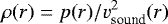 (1)
(1)
with vsound the isothermal sound speed. Velocities in this deeper, photospheric part are derived from the continuity equation (solving Eq. (3) provided below for v(r)), using the density stratification from above. The resulting photospheric structure is smoothly connected to the wind outflow, at a pre-defined “transition velocity”, with a default value of 10% of vsound (evaluated at Teff for the specific composition). The wind-structure is specified by a typical β velocity law,
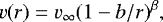 (2)
(2)
and mass-loss rate Ṁ (input),
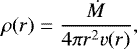 (3)
(3)
with terminal wind speed, v∞ (input), b a parameter calculated in parallel with the location of the transition point and the transition velocity, and β the input parameter controlling the steepness of the wind velocity field. In parallel to densities and velocities, a consistent temperaturestructure is determined, using a flux-correction method in the lower atmosphere, and the electron thermal balance (cf. Kubát et al. 1999) in the outer part.
Wind clumping
In our current v11 version as described here, we “only” allow for conventional, optically thin wind clumping, consistent with many earlier versions of FASTWIND. A variety of stratifications for the clumping factor, fcl (r) (= overdensities in clumps, if the interclump medium is assumed to be void) can be chosen by the user (or, if desired, newly defined). These include (i) spatially constant clumping factors from a pre-defined velocity on, (ii) the default parameterization of CMFGEN (Hillier & Miller 1999; Hillier et al. 2003), and (iii) generalizations of the latter (see Najarro et al. 2011). An implementation of optically thick wind clumping and porosity in velocity space, as already included in v10.3 (see Sundqvist & Puls 2018, and references therein) into our new v11 – more precisely, into the corresponding module – is foreseen for the near future. Because of its higher complexity (compared to optically thin clumping), careful tests preceeding a final release are required though.
NLTE and radiative transfer in FASTWIND v10
Within our previous FASTWIND version(s), the concept of “explicit” and “background” elements is used, as outlined in the introduction. The explicit elements are then treated straightforwardly and with high precision, namely by solving the NLTE rate equations and performing the line transport in the comoving frame (CMF), though neglecting explicit line overlap effects. Regarding the background elements, the procedure is more complex (for a schematic representation, see Table 1).
At first, we divide them into two subgroups, and call the more important ones – essentially those with a higher abundance – “selected” background elements. Currently, and if not included in the explicit elements, these are C, N, O, Mg, Ne, Si, P (because of its important UV-line), S, Ar, Fe, and Ni, but other elements of interest can be included into this list as well.
Whereas the occupation numbers of the remaining, “non-selected” elements3 are estimated via an approximate NLTE approach (Puls et al. 2005), for the selected ones we solve the detailed NLTE rate equations (as for the explicit elements). To save time, however, the required radiative bound-bound rates are calculated in three different ways: for the most important (strongest) transitions, we again solve the CMF transfer; for the weaker lines, the bound-bound rates are either approximated from a Sobolev approach (including the pseudo-continuum radiation field, see below), or, in the photospheric regime, derived from a static radiation transfer. All this only for individual lines, again neglecting specific line overlaps, except regarding transitions collected within the pseudo-continuum.
This pseudo-continuum, which is required to correctly describe line-blocking and blanketing effects, is obtained by sampling (almost) all individual opacities and source functions to continuum-like quantities (accounting for Doppler-induced frequency shifts in an approximate way), which are then used to solve the radiation transfer in the observer’s frame (cf. Puls et al. 2005). The resulting radiation field serves as input for a variety of calculations (such as approximate NLTE – see above – pseudo-continuum background for the Sobolev line rates, scattering continuum emissivity for the detailed CMF transport, radiative bound-free rates for exact NLTE calculations, bound-free heating and cooling rates, and photospheric radiation force), and the circle is closed.
2.2 Comoving frame transfer in Fastwind v11
The major change between the previous and the current FASTWIND version concerns the radiative transfer. In a new module, almost all lines and continua (both from explicit and background elements) are now treated in the CMF, thus allowing us to increase the precision, particularly by “automatically” accounting for line-overlap effects (both due to coincidental identities or similarities of transition frequencies, and wind-induced, cf. Puls 1987). This complete CMF transport is performed inside a wavelength range λmin to λmax, where, in the current version, the default values are 200 and 10 000 Å, respectively. Extending λmax to the near infrared (NIR) will be tested in future work. For late B-types and cooler (with vanishing He II ionization edge), λmin might be set to 400 Å, whereas for the hottest O-subtypes, it might be extended to lower values, for example, 130 Å, to include the N V edge. Test calculations have shown that such extensions do not change current results using our default value of 200 Å though. Outside the range λmin to λmax, we follow our previous, pseudo-continuum approach, but always check that the transition between both regimes is monotonic, and that no jump occurs (for an example regarding λmax, see Fig. A.2. Black: detailed CMF transport; green: pseudo-continuum approach). In these outer frequency domains (until X-ray frequencies in the blue, and radio frequencies in the red), all line-rates are calculated as in the previous versions described above.
Subsequently, our current approach solves the NLTE rate equations, for both explicit and selected elements, with radiative rates calculated from the detailed CMF transport. Thus, in the new code the most important difference between explicit and selected elements is now the source of atomic data, either flexible (explicit elements) or fixed (see Sect. 1). Once the atomic data are incorporated, the method makes (almost) no distinction between explicit and selected elements when solving the rate equations and the radiative transfer (again, see Table 1). The only additional difference refers to the degree of precision aimed at. Selected elements are considered as converged by following the changes within the ionization fractions, whilst for the explicit elements, all levels have to fulfill the required convergence criterion (see also Appendix B). Thus, the accuracy of specific excited levels might be higher when a certain element is treated as an explicit one, in the original spirit.
For the remaining (non-selected) background elements (also with fixed-format atomic data), the approximate NLTE approach is still in use, where the required radiation field quantities are taken from a re-mapped CMF solution (see Appendix C.1). Opacities and emissivities inside the CMF transport comprise all elements.
The CMF transport itself can be solved in two ways. Either, we perform a formal (“ray-by-ray”) solution for the Feautrier variables alone (applying a fully implicit scheme, following Mihalas et al. 1975, in the conventional p-z geometry, for example Puls et al. 2005; Puls 2020, and references therein), or – this is the default – we calculate the corresponding Eddington factors and solve the moments equations subsequently. To avoid numerical problems, and following Hillier & Miller (1998, their Eq. (13), with ɛ = 1), we apply the ratios of third to zeroth moment, Nν∕Jν, instead of the more commonly used ratios of third to first moment, Nν ∕Hν. In specific cases, particularly for (almost) vanishing fluxes, the former approach results in a more stable solution.
The reason for considering the moments equations is twofold. First, the solution for the angle-dependent Feautrier variables is affected from certain approximations related to the (standard) discretization on the p-z grid, such that specific intensities and corresponding moments (particularly flux-like quantities) suffer from inaccuracies. Since these inaccuracies mostly cancel within moment ratios, a subsequent solution of the moments equations can provide a more exact outcome. Moreover, by definition, such a solution needs to be performed only on the radial grid, and thus is computationally inexpensive.Comparing the results for a comprehensive model grid (see Sect. 3, and Table 2) from both methods has revealed that the differences in the emergent spectra in most cases are marginal, and only the temperatures at large optical depths (which are irrelevant for most applications) can be affected to a non-negligible extent.
The second reason for additionally solving the moments equations refers to computational performance. As long as the majority of occupation has not stabilized close to our convergence criterion (on the order of few per mille), which in our scheme is true as long as the temperature structure of the atmospheric model has not converged (see Appendix B), it is suitable to fix the Eddington factors within one to three subsequent iterations. Then, we can solve the moments equations alone, without any formal solution. (In later iteration stages, such a fixing would be (slightly) inconsistent, and would destroy the final convergence of sensitive transitions). Fixing the Eddington factors (when possible) decreases the computational time significantly, since the otherwise required angle-dependent CMF transport is the most time-consuming part of the total calculation. This, because it scales with the number of radial grid points, the number of p-rays, and the large number of frequency points, Nf, to be considered. For given (fixed) Eddington factors, on the other hand, the moments equations scale “only” with the number of radial grid points, and Nf.
The latter primarily depends on the assumed micro-turbulent velocity, vmic, and can be estimated4 by
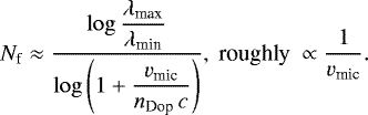 (4)
(4)
For our default values, and nDop the number of frequency points per Doppler-width (=3 in our simulations), this results in Nf ≈ 230 000 and Nf ≈ 710 000 for vmic = 15 and 5 km s−1, respectively, which are prototypical values for O-supergiants and B-dwarfs.
As a last, more technical aspect, we approximate the incident intensity at the outermost grid point, I− (and its frequency derivative), as described in Appendix A, to keep the computational effort as low as possible. This differs from the CMFGEN approach as introduced by Hillier & Miller (1998), namely to “extend” the atmosphere in the ray-by-ray solution toward larger radii and optically thin conditions (using extrapolated opacities and emissivites), and then set I− to zero at the new, extended boundary.
Stellar and wind parameters of our model grid used to check specific details of our new FASTWIND version (v11), and to compare with results from CMFGEN and FASTWIND v10.
2.3 Accelerated lambda iteration, and approximate lambda operators
To improve (or even enable) the convergence of our solution scheme, we apply, as already done in FASTWIND v10, an accelerated lambda iteration (ALI), contrasted to CMFGEN that uses a linearization method. The required, approximate lambda operators (ALOs), are calculated in parallel with the ray-by-ray solution, following Puls (1991).
We stress here that the actual ALO entering the pre-conditioned (Rybicki & Hummer 1991; Puls 1991, denoted by “reduced” in the latter work) radiative bound-bound rates needs to be weighted at each frequency (before integration over the profile function), due to the manifold line-overlaps. The weighting factor is given by the ratio between the line opacity of the considered transition, i, and the total line opacity present in the CMF transfer at frequency ν. This is necessary since the ALO constructed by our method refers to the total line source function entering the radiative transfer (the contribution by continuum processes is seperately accounted for), whereas the pre-conditioned line rates refer to the individual ones, related via
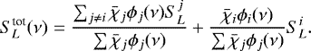 (5)
(5)
Because the approximate lambda operator, within the bound-bound rates, needs to act on the line-specific source function,  (frequency independent, when assuming complete redistribution), it must be weighted by the fore-factor of the second term in Eq. (5). In this equation,
  is the frequency dependent line opacity for transition j (with 1…i…j overlapping components), and ϕj(ν) the line profile function5.
As outlined above, our solution scheme does not only use the ray-by-ray solution, but also the corresponding moments equations. Since, however, the latter yield slightly different mean intensities than the former, in principle it might be necessary to calculate a second set of approximate lambda operators (ALOs) which are consistent with the solution of the moments equations, and thus can be used in parallel with the corresponding scattering integrals, 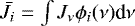 , within the (pre-conditioned) radiative bound-bound rates. Contrasted to the case of static radiative transfer, however, the development of optimum ALOs within the CMF transport is quite complex (due to the presence of the frequency derivatives), and, thus far, has been performed only for the angle-dependent, formal solution (Puls 1991). A corresponding ALO to be calculated in parallel with the moments equations is, to our knowledge, still not available (though certainly possible).
Fortunately, and after many tests, it turned out that it is sufficient to use the ALOs from the ray-by-ray solution, even if the  ’s have been calculated from the moments equations. Only in those cases when the ALOs are very close to unity (> 0.99 in our implementation using diagonal operators), we reset them to the latter value, to account for potential inconsistencies. Such a reduction is “allowed,” since lower than optimum diagonal operators do not lead to a divergence of the ALI, contrasted to overestimated ones (see Olson et al. 1986). On the other hand, whenever sub-cycles with fixed Eddington-factors are performed (see Sect. 2.2), the ALOs need to be set to zero, since otherwise the occupation numbers would be strongly disturbed, due to the somewhat inconsistent approach. Since the latter cycles appear only at earlier stages of the calculation (before the temperature structure has converged), a neglect of the ALO does not play a role though. This even more, since each second to fourth iteration is still performed with both solutions (ray-by-ray and moments), such that at this stage a consistent ALO becomes known, and speeds up the convergence again. Details on the overall iteration cycle and convergence properties are outlined in Appendix B.
2.4 Additional issues
In the following subsection, and also Appendix C, we discuss additional issues which are important for our specific FASTWIND implementation.
Formal integral
After the model and all occupation numbers have converged (or quasi-converged, when oscillating, see Appendix B), we calculate, in a separate program package, the formal integral in the observer’s frame to obtain (normalized) synthetic spectra. Basically, we follow our approach from Santolaya-Rey et al. (1997) of interpolating opacities and emissivities onto a spatial micro-grid (in z), with a typical resolution corresponding to Min(vmic(r))∕3, but we abstain from a separation of continuum and line processes6, and integrate over total opacities and source-functions. The latter are calculated in the spirit of Hillier & Miller (1998). Namely, before any interpolation, the line list (for background and explicit elements), the occupation numbers, and continuum opacities and emissivities are re-stored from the last iteration of our NLTE-model calculations. Subsequently, corresponding total opacities and emissivities are derived, still at comoving-frame frequencies (that is, without anyvelocity field induced Doppler-shifts), by summing up line and continuum quantities. At this point, all relevant broadening mechanisms (see below) are accounted for. This calculation has to be performed only once, and is quite fast, since it needs to be executed only on the coarse radial grid, and for the spectral range defined by the user (see below). Only after the total opacities and emissivities have been calculated (and stored), they are interpolatedonto the spatial micro-grid, and evaluated at the corresponding local comoving frame frequency (again by interpolation), in dependence of rest-frame frequency and projected velocity. Specifically, if the local CMF frequency is νCMF(z) ≈ νobs(1 − μv(z)∕c), then the opacities and emissivities have to be interpolated from the pre-calculated values (see above) at CMF frequencies  , if the (unshifted) CMF-frequency grid has indices i, and μ is the cosineof the angle between radial and radiation direction.
After the formal solution for the specific intensity has been derived (for all considered rest-frame frequencies, and all impact parameters, with a default value of 80, inclusive 10 core rays), the frequency-dependent emergent fluxes can be calculated by angular integration. The normalization is finally obtained by calculating one additional formal solution, accounting for the continuum opacities and emissivities alone (no micro-grid required here), and dividing the total emergent fluxes by the continuum ones. The range and resolution of the synthetic spectra can be specified by the user (default: 900–2000 Å and 3400–7000 Å, with a resolution of 0.1 Å), as well as the micro-turbulence. For the latter, either a constant or depth-dependent value can be chosen (to simulate the effects of the large velocity dispersion seen in hot-star instability simulations, and observed through the so-called black troughs in saturated UV P-Cygni lines, see Hamann 1980; Lucy 1982; Puls et al. 1993; Sundqvist et al. 2011a). To compare with previous models, and to obtain an impression about the impact of blends from other elements, our program package allows us to also calculate individual line profiles for specified transitions within the explicit elements, identical with the approach followed by FASTWIND v10. Finally, we note that line-broadening is accounted for in the standard way, using Stark broadening for the hydrogen and helium lines, and Voigt profiles (with damping parameters derived from data collected in the LINES.dat file, see Appendix C.2) for the metals. If no broadening data are available (as for Fe and Ni in our current data-base), simple thermal and micro-turbulent broadening is adopted.
Level dissolution
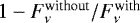
Contrasted to CMFGEN and some other NLTE-codes dedicated to hot star atmospheres, the new FASTWIND version does not account for level dissolution (Hummer & Mihalas 1988; Hubeny et al. 1994). By switching off such processes in CMFGEN, and comparing with its standard treatment including level dissolution, we have convinced ourselves that in most cases the corresponding emergent fluxes do not differ substantially, except (very) close to the Lyman and Balmer edges. Indeed, larger variations begin, for model d6v, only for Lyman (and corresponding He II) transitions with an upper principal quantum number, nu ≥ 8 (λ≲926 Å), and for Balmer transitions with nu ≥ 11 (λ≲3770 Å), whereas the transitions close to the Paschen threshold display only moderate effects. Generally, the dwarf models, because of a higher density at typical line-formation depths, display larger effects than supergiant models, as visible in Fig. 1. In this figure, we have excluded the Lyman range below 930 Å, and the Balmer range below 3700 Å, to allow for a better vertical resolution of the diagnostic wavelength regimes. Typical deviations in the line cores are, for a dwarf model, on the order of less than 1% in the UV, and on the order of 0.3–0.5% in the optical and NIR. For supergiant models, the differences are even lower. Thus, we conclude that except for a realistic representation close to strong ionization edges (in particular, Lyman and Balmer), and potentially for corresponding lines between high-lying levels (in the far infrared and radio regime), our neglect of level-dissolution effects does not lead to significant inaccuracies (at least if we will not apply our code to white dwarfs). However, the above restrictions should also prevent the user from “blindly” applying our new FASTWIND version, for example, for estimating the Balmer-decrement, or for constraining the gravity from the very high series members close to corresponding ionization edges.
 |
Fig. 1 Effects of level dissolution in the UV (left) and the optical and NIR (right), for models s8a and d6v (see Table 2). Displayed is the deviation of the emergent fluxes,
|
2.5 Computation time and memory requirements
As already mentioned, the major fraction of computational time within our implementation is typically spent for the ray-by-ray solution, which increases almost linearly with 1∕vmic. For our standard set-up (see Sect. 3.1), with H, He, and N as explicit elements, and 67 depth points, a program run with 140 iterations requires 1.2 and 1.6 CPU hours on an Intel Xeon processor with 3.7 and 2.7 GHz, respectively, if we use vmic = 15 km s−1, and 3.2 vs. 4.4 CPU hours for vmic = 5 km s−1. For the same specifications, 1.6 GB RAM needs to be allocated, which is comparatively modest. We tried to keep the required RAM as low as possible, to allow us to calculate as many models as possible in parallel (comments on a future parallelization are given in Sect. 5).
Since models with H and He as explicit elements converge much faster (typically, after 80 to 100 iterations7), they require “only” 1 CPU hour on a 2.7 GHz machine, for vmic = 15 km s−1. Already such model types are well suited to calculate the total radiative acceleration required for self-consistent massive star wind models (Gräfener & Hamann 2005; Krtička & Kubát 2017; Sander et al. 2017; Sundqvist et al. 2019, the latter authors already using the new FASTWIND version), and also the UV spectrum of hot stars.
The formal integral, on the other hand, has much shorter turnaround times, due to the frequency and spatial interpolation of the total CMF opacities and emissivities. For our default parameters for spectral range and resolution (see above), the typical execution times are on the order of 5 to 15 min, mostly depending on maximum wind speed (and processor frequency). To calculate individual line profiles for strategic lines from explicit elements, the turnaround times are even shorter. If we resolve each line by 161 frequency points, the most important strategic lines from H, He, and N are calculated in less than one minute.
3 First results, including comparisons to CMFGEN and FASTWIND v10
Most tests of our new FASTWIND version have been performed for stellar and wind parameters as defined by a model grid that covers early B to hot O-type dwarfs and supergiants below Teff = 47 kK. This grid also served for comparing with analogous results from CMFGEN models. The latter (for the same grid-parameters) have been calculated by one us (F.N.), with a recent CMFGEN version that solves the hydrostatic equation in the inner atmosphere, and which has also been slightly modified to improve the transition between photosphere and wind (Najarro et al., in prep.). The grid itself is a subset of the grid introduced by Lenorzer et al. (2004), and has already been used in previous comparisons by Puls et al. (2005) and Rivero González et al. (2011, 2012b). For convenience, grid parameters and basic assumptions are repeated in Table 2.
3.1 Default specifications used for the model grid
To enable a basic check, and to avoid the impact of additional effects, in the following we concentrate on models with homogeneous (unclumped) winds, and without X-ray emission from wind-embedded shocks. Specific aspects of the latter will be discussed in Sect. 4. We use H, He, and N as explicit elements, unless explicitly stated otherwise. The corresponding atomic models are identical to those used in FASTWIND v10. Details regarding H and He have been presented in Puls et al. (2005), and our nitrogen model atom has been discussed in Rivero González et al. (2012a). For the model-atmosphere calculations, we use a (default) grid of 67 carefully distributed radial depth-points, and for the p− z geometry, a set of 77 impact parameters, including 10 core-rays (a similar8 set of 80 impact parameters is used in the formal integral). Tests have shown that these numbers are sufficient to obtain a reasonable resolution, and negligible errors in the angular integrations. For supergiant atmospheres with a denser wind, even a reduction to 51 depth points (with 61 impact parameters) is possible, without loss of significant information.
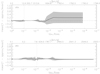 |
Fig. 2 Mean (relative) differences between the main ionization fractions as predicted by our approximate NLTE description following Puls et al. (2005), and our current “exact solution” (complete NLTE, detailed CMF transport), as a function of τRoss ≤ 1 and v (in km s −1). Displayed are the models with the largest differences (s6a) and the smallest ones (d6v) within our grid. The mean (see Eqs. (6) and (7)) refers to 11 selected elements from C to Ni, and its 1-σ deviation is displayed in gray. The vertical lines indicate the location of the sonic point. |
3.2 Approximate versus detailed treatment
Our new method allows us to repeat a test already performed with an earlier FASTWIND version (cf. Puls et al. 2005, their Figs. 5 and 6), namely to evaluate the reliability of our approximate NLTE description. As explained earlier, this description is still in use for the non-selected background elements, which play a certain role, for example, for defining the (line-blocked) radiation field, and the temperature structure. For this test, in Fig. 2 we compare the mean relative differences between the main ionization fractions predicted by the approximate method, and our current, exact NLTE approach using a detailed CMF transfer,
![Mathematical equation: \begin{equation*}\left\langle \left(1-f_{k, \textrm{approx}}^{\textrm{max}}/ f_{k, \textrm{detailed}}^{\textrm{max}}\right)\right\rangle= \frac{1}{N_k}\sum_{k \in [3,30]} \left(1-f_{k, \textrm{approx}}^{\textrm{max}}/ f_{k, \textrm{detailed}}^{\textrm{max}}\right), \end{equation*}](/articles/aa/full_html/2020/10/aa38464-20/aa38464-20-eq11.png) (6)
(6)
with  the maximum ionization fraction for element k,
![Mathematical equation: \begin{equation*}f_{k}^{\textrm{max}}=\textrm{Max} \left(\frac{n_{jk}}{n_k}\right), \quad j \in [1,j_{\textrm{high}}(k)]. \end{equation*}](/articles/aa/full_html/2020/10/aa38464-20/aa38464-20-eq13.png) (7)
(7)
Here, nk is the total population of element k, njk the population of ion j, and jhigh(k) the highest ionization stage considered for element k.
The mean itself is evaluated for our default set of Nk = 11 selected background elements (see Sect. 2.1), and is displayed as a function of τRoss ≤ 1 (since the differences for larger τRoss vanish anyhow, due to thermalization), and of velocity. Due to the negligible computational effort, we can easily perform this test, since at each iteration we anyhow calculate the approximate NLTE occupation numbers for all background elements, before replacing those for the selected elements by their exact counterparts9. After inspection of all our grid models, it turned out that the largest differences occur for model s6a (in the outer wind), and the smallest ones for model d6v. Both cases have been displayed, including the 1-σ scatter of the mean. For all our models, the approximate treatment provides satisfactory results in the photosphere, whereas larger deviations (with a mean difference up to 20%, and a large scatter) are possible in the outer wind. Nevertheless, even these deviations are still tolerable, and we conclude that our approximate NLTE approach is acceptable if one is interested in gross effects such as line-blocking opacities, and maybe even radiative line-accelerations, at least if derived via detailed radiative transfer calculations. All this of course only if the (pseudo-) continua are calculated in a reasonable way, comprising line-blocking effects.
Without appropriate pseudo-continua, the ionization fractions would certainly become erroneous (because of erroneous ionization integrals, be them calculated in an approximate or exact manner). Thus we have to check the differences between our previous (continuum-like background opacities, observer’s frame transport) and current (detailed CMF-transport) approach. Again, for all our models, a fair agreement is found, where a prototypical example is displayed in Fig. A.1, left panel.
3.3 The He I singlet problem
Already in our very first runs of the new program version, we encountered the same problem as first described by Najarro et al. (2006), the so-called He I singlet problem, resulting from a specific line-overlap effect between the He I resonance line at roughly 584 Å and a few close lying Fe IV lines (and, potentially, lines from other elements). If the Fe IV lines have oscillator strengths as found in current data-bases (on the order of ≳10−3, for details, see Najarro et al. 2006), the line overlap leads to a lower population (compared to the case without overlap) of the He I 1s2p1Po level. This, in turn, is the lower level of important diagnostic lines of the He I singlet series in the optical, such as He I 4387, 4922, and 6678 Å, and the upper level of He I 2.058 μm in the K-band. Due to the lower population, the optical lines become weaker (again: compared to the case of no overlap), or even appear in emission, whereas the K-band line becomes stronger. This behavior was particularly found in CMFGEN models, whereas previous FASTWIND versions produced comparatively stronger optical lines (in agreement with observations), because of the neglect of detailed line-interactions. Now, with the new FASTWIND version, very similar effects and He I singlet profiles as in CMFGEN are predicted, telling us that both the results from FASTWIND v11 and CMFGEN and the involved atomic data are consistent, and enforcing our confidence in the new approach. To achieve consistency with observations, we “cured” the problem in a similar way as suggested already earlier by co-author Najarro (priv. comm), namely by reducing the (still quite uncertain) oscillator strengths of the involved Fe IV transitions to a lower value (gf = 10−5, with gf the product of oscillator strength, f, and statistical weight of the lower level, g). With such a reduction, the impact of the Fe IV lines decreases significantly, and the resulting optical He I singlet lines become stronger again, in agreement with the predictions by our previous FASTWIND version. Certainly, this problem needs to be rechecked, when new atomic data calculations become available. Here, we again warn about concentrating on these singlet lines within quantitative spectroscopy: abundances, ionization conditions, and micro-turbulent velocities, in combination with somewhat insecure Fe IV transition frequencies, can affect the strength of the overlap, and lead to additional uncertainties. Thus, we recommend to prefer the results from the much more stable He I triplet lines.
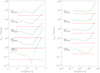 |
Fig. 3
|
3.4 Radiative acceleration
Figure 3 compares the total radiative acceleration as calculated by FASTWIND v11 and CMFGEN, measured inunits of gravitational acceleration, and as a function of velocity. Thus, it displays Eddington’s Γtot. The red dashed-dotted lines indicate the conventional Gamma-factor for electron scattering, Γe. For the supergiants, both codes agree almost perfectly, while for the dwarf models, a certain deviation in the transonic region is present. The major reason for this discrepancy is most likely related to the different treatment of the transition between photosphereand wind (in particular, corresponding velocities and gradients), and to the different line lists. Even for these models, however, the accelerations in the wind agree very well.
For the coolest dwarf model (d10v), FASTWIND predicts a (slightly) negative total acceleration above the transition point, but also in CMFGEN the total (still positive) acceleration is lower than Γe, indicating a larger inward- than outward-directed line acceleration, due to negative fluxes from above (resulting from strong wind lines that are not present in the transition regime).
Given that both codes use a largely different philosophy, and different atomic data bases, the overall agreement is remarkable though. We note that for all models, Γtot = 1 is reached only at substantial velocities (100 km s−1 or more), whereas, in realistic wind-models, this should happen very close to the sonic point (20–25 km s −1). Thus, the displayed models are far away from being hydrodynamically self-consistent. By iterating the radiative acceleration and the resulting wind-structure to relax at constant mass-loss rate, velocity structure, and Γtot ≈ 1 at the sonic point10, Sundqvist et al. (2019) used the current FASTWIND version to obtain such self-consistent models. As it turned out, a quite steep velocity field in the transonic region and the lower wind is required to fulfill the latter condition (see also Krtička & Kubát 2017; Sander et al. 2017 for similar approaches, the latter performed with PoWR). Moreover, the negative Γtot-values found here for the coolest dwarf model (invoking a β velocity law) vanish when iterating for the radiative acceleration. The characteristic “force-dip” (the decrease in acceleration before its increase in the wind) remains always present though.
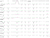 |
Fig. 4 Comparison of strategic H and He lines in the optical, for all models from our grid. Black: FASTWIND v11, green: CMFGEN, red: FASTWIND v10, with no blends from other elements. The marker in the lower right indicates a wavelength range of 20 Å, and a vertical extent of 0.5 of the continuum. To enable a better comparison, the spectra have been convolved with a rotational broadening of v sin i = 80 km s−1, and degraded to a resolving power of 10 000. |
3.5 The optical hydrogen and helium spectrum
In Fig. 4, we compare important diagnostic hydrogen and He I, He II lines in the optical, in the upper sets with results from CMFGEN (in green), and in the lower ones, with results from the previous FASTWIND version, v10 (in red). The HHe spectra from our new FASTWIND version have been derived by including all overlapping lines that are present, whereas those from the old version account only for H, He, and N components. Both CMFGEN and FASTWIND v11 models have been calculated with a diminished influence of the Fe IV line(s) overlapping with He I 584 (see Sect. 3.3).
Again, the agreement (also for blends from the other elements) is almost perfect, and even the shape of the Hα and He II 4686 wind emission coincides impressively. The only problem which was and still is present refers to the cores of He II λλ4200-4541, which, in the temperature range between 30 to 36 kK, are stronger in CMFGEN, and lead to somewhat different effective temperatures when analyzing hot star spectra by means of one code or the other. Though this discrepancy has become slightly milder when comparing with the new FASTWIND version, the overall difference remains. The agreement between the previous and current FASTWIND version, on the other hand, is excellent, and results from previous diagnostics should remain (almost) unaltered. A tiny reduction in Teff, on the order of few hundred Kelvin (toward the lower values implied by CMFGEN) might be possible though, in the temperature range outlined above.
3.6 The optical N III spectrum, and the formation of N III λλ4634–4640–4642 revisited
In analogy to the previous section, in the following we compare our current results for nitrogen, the third explicit element considered, with results from alternative simulations, as an example for elements where diagnostic lines in the optical are affected by line overlaps in the extreme ultraviolet (EUV). In particular, we revisit the formation of N III λλ4634−4640−4642, which was already discussed by Rivero González et al. (2011), though with respect to our previous FASTWIND version.
Figure 5 displays the comparison with CMFGEN (in green) and FASTWIND v10 (in red), and it is immediately clear that the almost perfect agreement found for the H and He lines is no longer present, though in most cases there is still a nice qualitative concordance. Particularly N III 4003 and N III λλ4510−4514−4518 (from the quartet system) are also in quantitative agreement, whereas N III 4379 is strongly contaminated by N II, O II, and C III, which makes a clean comparison with FASTWIND v10 (and the spectroscopic analysis) difficult. The often used diagnostic line N III 4097 (in the blue wing of Hδ) is predicted to be much stronger at hotter temperatures (compared to CMFGEN) by both FASTWIND versions. Particular differences are present for the (in-)famous N III triplet around 4640 Å, where often the emission strengths predicted by either of the three codes differ quite significantly. Only for the coolest dwarf (d10v, d8v) and supergiant (s10a) models, where the triplet is still in absorption, there is satisfactory agreement (even for the neighboring, strong O II lines at4638.9 and 4641.8 Å). The largest discrepancies are found for models s8a and d6v, where CMFGEN predicts weak emission, while FASTWIND predicts weak (v11) or stronger absorption (v10), and particularly for model s6a, where FASTWIND v10 predicts absorption, while v11 predicts moderate, and CMFGEN considerable emission.
Since model s6a was already scrutinized by Rivero González et al. (2011), and displays the largest differences between v10 and v11, we have re-investigated the line formation process of the triplet lines using the new capabilities of v11. In Rivero González et al. (2011), it was argued that the discrepancy between CMFGEN (N III triplet in emission)and FASTWIND v10 (N III triplet in absorption) is due to the line overlap between one component (at 374.434 Å) of the N III EUV resonance lines pumping the upper level of the optical triplet transitions (3d), and one component (at 374.432 Å) of the O III resonance lines in the same wavelength region (cf. insert of Fig. 6, right panel). Since, at typical formation depths of the triplet lines, and for atmospheric conditions similar to model s6a, the O III resonance line source function is stronger than the N III one, the pumping of N III 3d becomes more efficient than when the O III line is absent (for details, see Rivero González et al. 2011, their Sect. 7), and the optical N III triplet appears in emission. If, on the other hand, detailed line overlap effects are not included (as in FASTWIND v10), the triplet remains in absorption. We note that the discussed effect is particularly strong for Teff between 30 to 33 kK,whereas for hotter temperatures, the O III source function becomes weaker than the N III one. At such temperatures, the pumping by the N III resonance lines alone is sufficient to overpopulate the 3d level and drive the N III triplet into emission.
Now, with the new version, all these effects are “automatically” accounted for, and, indeed, the corresponding optical lines appear in emission (Fig. 6, left panel, black profiles)11. To check the arguments from Rivero González et al. (2011), we have artificially shifted N III 374.434 by a small amount to avoid the overlap, and, as predicted, the triplet components then appear in absorption (red profiles). Our argumentation would also imply that, if we alternatively decrease the oxygen abundance significantly (say, down to ɛO = 5), the emissionshould vanish as well. To our astonishment, however, the corresponding test (blue profiles) did not confirm our expectation,and the lines remained in emission. After carefully checking all processes, it turned out that, in the decisive EUV wavelength range, there is one more strong Fe V line, which can couple with one of the other components of the N III resonance multiplet (at 374.198 Å, see again insert), and, due to the large mean intensity in this line, now plays the role of oxygen when the latter is no longer present. Only if the Fe V line is excluded from radiative transfer, the nitrogen triplet turns, for low ɛO, into absorption (green).
The lesson to learn from this exercise is that for certain transitions which indirectly depend on EUV lines, there is always the chance that line-overlap effects can have a large impact, because of the high line density in the EUV regime. And since (as already argued with respect to the He I singlet problem) the strength of the overlap strongly depends on abundances, ionization conditions, micro-turbulent velocities, and velocity field gradients, which control the line optical depths and source functions, a variety of combinations can lead to a variety of (non-monotonic) results.
To examine the impact of vmic, we display a comparison for three models calculated with vmic = 15 km s−1 (standard), 10 km s−1 (red), and 5 km s−1 (blue) in Fig. 7. To allow for a fair comparison of the impact on the occupation numbers alone, in all three cases the formal integrals were solved with the same (standard) value for vmic. Obviously, the differences between profiles from models with vmic = 15 and 10 km s−1 are small, but for the lowest value, vmic = 5 km s−1 (empirically not supported for a supergiant at 33 kK), the emission decreases significantly. Here, because of the low micro-turbulent velocity, the profile functions become considerably narrower, and the coupling between the N and the Fe EUV resonance lines vanishes completely, whereas also the coupling between the much closer N and O resonance lines becomes weaker, inducing a reduction of emission strength.
As a final example for the (potential) non-monotonicity mentioned above, we display, again for models s6a, the reaction of the emission strength of the optical N III triplet on the oxygen abundance in Fig. 8. For abundances increasing until ɛO = 8.1 (and “normal” ɛFe), also the emission strengths increase, though only moderately (Fe V!). For larger values, when oxygen starts to dominate the line overlap even in the presence of Fe V, the emission begins to decrease, until, at ɛO = 9.5 (strongly super-solar), the lines appear in strong absorption. In this case, the source function of the oxygen resonance line, because of larger optical depths also in connected transitions, has changed its stratification in such a way as to prohibit effective pumping of the 3d level.
Consequently, we advise to put, if at all, only low weight onto the triplet lines when analyzing the nitrogen spectrum; if it fits, then fine, but if it does not fit, one might not conclude that there is something “rotten.” After all, and as shown above, the emission strength might depend, for example, on the oxygen and iron abundance, and not on the nitrogen abundance (the quantity which needs to be derived) alone, even if the impact of micro-turbulence is left aside.
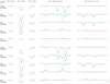 |
Fig. 5 As Fig. 4, but for strategic N III lines. Here, the marker indicates a wavelength range of 2 Å, and 0.2 of the continuum. The positions of the individual components of N III λλ4634−4640−4642 of the cooler objects can be clearly seen in the red FASTWIND v10 profiles. Since most lines are weak, no rotational broadening has been applied. |
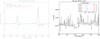 |
Fig. 6 On the formation of the N III λλ4634−4640−4642 emission lines in hot massive stars (here: model s6a, see Table 2). Left: optical emission lines (no broadening, no degrading) for various configurations of the EUV N III resonance lines (around 374 Å) coupled to the upper level (3d) of the optical transitions. See legend, and text. “[X]” means ɛX. Right: corresponding EUV radiation field, Jν(τRoss = 0.24). The insert displays the decisive region, and participating lines. Red: N III resonance lines (three components); green: overlapping O III resonance line (out of a multiplet of 6 components); blue: Fe V line at 374.245 Å. We note that 0.01 Å correspond to 8 km s −1. |
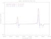 |
Fig. 7 As Fig. 6, left, but for different micro-turbulent velocities in the NLTE model calculations. To allow for a meaningful comparison of the impact on the occupations numbers alone, the micro-turbulent velocities in the formal integrals have been fixed at 15 km s −1 for all cases. |
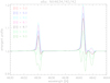 |
Fig. 8 As Fig. 6, left, but for different oxygen abundances (see legend), and “normal” Fe content. We stress the non-monotonic behavior. For increasing ɛO, the emission strength at first increases (until ɛO = 8.1), and then decreases, until strong absorption is produced (for ɛO = 9.5). |
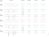 |
Fig. 9 As Fig. 5 (same scale), but for strategic N IV and N V lines of our hotter models. The blue profiles correspond to models, where specific EUV transitions feeding the lower and upper levels of N IV 6380 and of N V λλ4603-4619 have been treated as isolated lines, i.e., ignoring blends. See text. |
3.7 The optical N IV and N V spectrum
As a last comparison of optical spectra, Fig. 9 displays important diagnostic lines from N IV and N V, for those models where these lines are visible. For N IV, the agreement between FASTWIND v11 and CMFGEN is satisfactory, though for the hottest models the emission strength of N IV 4058 and the absorption strength of N IV 6380 are larger when calculated via FASTWIND. Compared to the older version v10, the agreement is of similar quality; only for specific models (s4a and d2v) there are larger discrepancies. Interestingly, there are no other (dominating) lines interacting with the EUV resonance lines feeding the upper and lower levels of N IV 6380. This is visible when comparing with the profiles in blue, calculated by treating these lines as isolated, that is, discarding any direct overlap effect12.
For close-to-solar nitrogen abundances, only the hottest models (d2v and s2a) display well-developed optical N V λλ4603-4619 profiles, sometimes with additional, blue-wing wind absorption. These lines can serve as important diagnostics for the effective temperatures of the earliest O-types (for example, Rivero González et al. 2012b), and were shown, within FASTWIND v10, to agree with results from CMFGEN (also visible in Fig. 9).
On the other hand, the N V lines (at least when comparatively strong) do no longer agree with CMFGEN when calculated with the new version v11. Indeed, they now are stronger (black versus green profiles in Fig. 9), and thus also stronger than predicted by v10 (black versus red). As for N IV 6480, also the N V profiles are barely affected from EUV resonance line overlaps (black versus blue), and such effects cannot be “blamed” for being responsible for the apparent disagreement. As it turned out, the discrepancy is, if (i) compared to CMFGEN, due to higher EUV fluxes around 266 Å (the wavelength of the N V 2 → 3 transition pumping the lower level of the optical N V lines). (ii) If compared to v10, on the other hand, the discrepancy originates from higher temperatures (in v11) in the transition regime between photosphere and wind. Consequently, v10 predicts lower N V ionization fractions, and thus weaker profiles. At our current knowledge, the agreement between v10 and CMFGEN is just coincidental, and it is difficult to estimate which prediction is closer to reality. More comparisonsbetween theory and observations for the hottest stars will certainly help to clarify this issue. Until then, we warn about taking synthetic optical N V line-profiles and strengths (from whatever code) at face value.
3.8 The UV range
In Fig. 11 below, we finally compare the region between 900 and 2000 Å, for the hot (d2v, s2a), intermediate (d6v, s6a) and cool (d10v, s10a) O- and early B-star regime. In the individual panels (two per model), we have indicated the rest wavelengths of important transitions from carbon to sulfur ions. The distribution of the ubiquitious Fe lines is displayed in Fig. 10, for the stronger lines (gf ≥ 0.1) of ionization stages IV, V, and VI relevant for our model grid. As is well-known, the line number decreases with increasing ionization stage, and, except for a common peak around 1000 Å, the different ions culminate in different ranges: Fe IV around 1200 Å, close to Lyα, and between 1500 and 1700 Å; Fe V between 1350 and 1500 Å; and Fe VI between 1200 and 1375 Å. Though Ni has similar line-densities, the impact on the (photospheric) background opacity is weaker, due to a lower abundance (factor ~18 lower than Fe for solar conditions).
To allow for a meaningful comparison, all spectra in Fig. 11 have been convolved with v sin i = 200 km s−1, since otherwise the multitude of narrow Fe lines would hamper such an effort. This is shown in Fig. 12, where a close-up of the region between 1210 and 1230 Å is displayed for convolved and non-convolved spectra.
For the hottest models, the agreement between FASTWIND v11 and CMFGEN is almost perfect (also regarding Fe V and Fe VI), and only for the supergiant model (s2a), some discrepancies for S V, the region close to Si IV, and the pseudo-continuum around 1600 Å are visible. We note that, in these models, O VI is clearly present in the wind (though far away from being saturated), even without any X-ray radiation field (cf. Sect. 4, and Carneiro et al. 2016).
Proceeding toward the intermediate models, the only “light” element which disagrees is sulfur, where FASTWIND indicates more S VI and less S IV, whereas S V coincides. In both codes, O VI has become purely photospheric, and the only additional differences refer to the iron forest around 1000 and 1200 Å, where CMFGEN predicts considerably more absorption. On the other hand, the region longward of C IV (dominated by Fe IV) agrees perfectly.
Considerable differences are present for our coolest models. Though the wind lines display a satisfactory agreement (with larger wind emission in FASTWIND, due to a weaker contamination by the background), the iron forest around 1000 Å, and particularly around 1200 Å (denoted by red dashes) is significantly stronger in the d10v model from CMFGEN. Indeed, the pseudo-continuum around Lyα is shifted to a level of ~60% of the true continuum, compared to a level of ~80% in FASTWIND (Fig. 12, upper panel). For the corresponding supergiant model, s10a, such a discrepancy is even present throughout the almost complete range shortward of 1700 Å.
Before providing further details, we stress that in concert with most strategic wind lines, also the P V line profiles perfectly agree for all our grid models, including those that are not displayed here. This implies that the predicted ionization fractions of phosphorus coincide perfectly, strengthening our confidence in using this line as a diagnostic tool to constrain the amount of velocity-space porosity induced by optically thick clumps (Fullerton et al. 2006; Oskinova et al. 2007; Sundqvist et al. 2011b, 2014).
In Fig. 12, we now investigate the origin of the discordance between the pseudo-continua within the cooler (but, for specific ranges, also the intermediate) models, by means of a close-up into the wavelength range between 1210 and 1230 Å, and model d10v. Whereas, in CMFGEN, more or less the complete range around Lyα is affected by photospheric line absorption, the spectrum predicted by FASTWIND coincides only for the stronger lines. In between these lines, however, many line-free regions are visible, comprising roughly 50% of the total range. These differences are responsible for the different pseudo-continuum flux-levels mentioned earlier.
Since the hotter models (including d4v and s4a) do not display such a discrepancy (if at all, FASTWIND predicts more Fe V absorption around 1600 Å), it is most likely that the origin relates to Fe IV. This expectation is confirmed when calculating (within CMFGEN) the formal integral excluding all Fe IV lines (red spectrum in the middle panel). In this case, only very few lines are still present in the considered spectral range, and the pseudo-continuum does not become depressed.
We have checked our Fe model atom, and realized that (at least) the 4d levels and corresponding transitions are missing. This certainly needs to be further investigated (work in progress). However, we also realized that just in the considered range around 1200 Å, the majority of lines synthesized by CMFGEN (including a multitude of very weak, overlapping ones) are due to transitions between energy levels that have been theoretically predicted, but, until to-date, not been observationally identified (in the following denoted as “non-observed levels”). In the range above 1700 Å, where CMFGEN and FASTWIND spectra agree, such transitions play only a minor role. When excluding all transitions between non-observed energy levels in Fig. 12, the result is quite similar to the case when excluding Fe IV completely (blue versus red spectra in the middle panel). We thus conclude that it is the multitude of such transitions that is responsible for the strong continuum depression.
Nevertheless, and irrespective of this discrepancy between synthetic spectra, there is another issue: for the displayed comparison, we have deliberately chosen model d10v (and not s10a, where the discrepancy is even larger), since (i), with Teff = 28 kK, it is not as contaminated by Fe III as model s10a (Teff ≈ 24 kK), and (ii), we can compare our results also to the high resolution COPERNICUS spectrum of τ Sco (B0.2 V), a well known object with very low rotation rate (close to zero, for example, Nieva & Przybilla 2012). The latter condition enables to record most individual photospheric lines that are actually present. The spectra, with a nominal resolution of 0.05 Å, have been taken from Rogerson & Upson (1977). We note that τ Sco is only slightly hotter than our grid model d10v (Repolust et al. 2005; Marcolino et al. 2009; Martins et al. 2012; Nieva & Przybilla 2012), which, in conjunction with its higher gravity, should result in similar ionization conditions.
From the lower panel of Fig. 12, red spectrum, it is evident that many of the actually observed lines are much weaker than predicted by both CMFGEN and FASTWIND. To demonstrate that this is not an effect of too large a micro-turbulent velocity (adopted as vmic = 15 km s−1 in our “standard” models), the turquois spectrum in the lower panel13 has been calculated with vmic = 5 km s−1, a value inferred from an optical analysis of τ Sco (Nieva & Przybilla 2012). Evidently, the discordance with the observations is still present. Moreover, various predicted lines are even absent in the observations. Wrong normalization is not likely an issue, at least around 1228–1230 Å,since the strengths of those lines that are simultaneously present in theory and observations are quite similar14.
One might argue that τ Sco is not well-suited for the above comparison, because of its strong and complex magnetic field (Donati et al. 2006). Indeed, the UV wind-lines seem to be significantly affected by the magnetic field (Petit et al. 2011), but the photospheric lines in the optical (from H, He, and various metals) are prototypical for non-magnetic stars of the given spectral type (for example, Nieva & Przybilla 2012). We thus expect that also the photospheric UV Fe-lines should be representative for normal conditions. Moreover, we checked τ Sco’s UV spectrum against the one from 10 Lac (Brandt et al. 1998), a non-magnetic star of similar spectral type (O9V). Both spectra turned out to be very similar, displaying only few lines in the range around Lyα. (We note that the few, actually present lines are somewhat shallower and broader in 10 Lac, because of its non-vanishing projected rotational speed.)
Thus, it is quite probable that both codes might overestimate the Fe IV line blocking (for such models where Fe IV is significantly populated) in certain wavelength regions, since many of the predicted lines from non-observed energy levels might not be present in reality. Of course, detailed comparisons with observations for a variety of objects are required to substantiate such a hypothesis, and, in case, to allow us to improve the atomic models and line-lists.
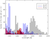 |
Fig. 10 Distribution of Fe IV,V,VI lines with gf ≥ 0.1 according toour line list, in the range between 900 and 2000 Å. See legend and text. |
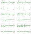 |
Fig. 11 Sythetic UV spectra from FASTWIND (black) and CMFGEN (green), for hot, intermediate, and cool O- and early B-star models. To allow for an easy comparion, all spectra have been convolved with v sin i = 200 km s−1. For model d10v, the range enclosed by red lines is detailed in Fig. 12. |
 |
Fig. 12 Close-up of the region between 1210 or 1220 and 1230 Å, for model d10v. In addition to the “standard” spectra from FASTWIND and CMFGEN (with vmic = 15 km s−1, as in Fig. 11), we display results from a FASTWIND formal solution with vmic = 5 km s −1, and two further sets where specific lines have been discarded from the formal solution in CMFGEN, namely either all Fe IV lines, or all transitions (i.e., from all elements) between energy levels that are predicted, but not observationally identified. For color coding, see legend. All spectra have been calculated with an intrinsic resolution of 0.01 Å or better. In the upper panel, they have been convolved with v sin i = 200 km s−1, as in Fig. 11, whereas in the lower ones no broadening has been applied. |
4 X-rays from wind-embedded shocks
Obviously, reliable UV diagnostics require a sufficient decription of the ionization balance of relevant atomic species. This balance can be significantly affected by X-ray emission from wind-embedded shocks. Already the first X-ray satellite observatory, EINSTEIN, has revealed that O-stars are soft X-ray sources (Harnden et al. 1979; Seward et al. 1979). Many subsequent and recent studies (particularly using Chandra and XMM-Newton) have improved our knowledge on corresponding features and processes (for a brief summary, see Carneiro et al. 2016). This X-ray (and EUV) emission is widely believed to originate in wind-embedded shocks, which in turn should be related to the so-called line-deshadowing instability, “LDI” (Lucy & Solomon 1970; Owocki & Rybicki 1984; Owocki et al. 1988; Owocki 1994; Feldmeier 1995). Due to both direct and Auger ionization (where, under prototypical conditions, the latter process only affects N VI and O VI, see Carneiro et al. 2016 and references therein), the ionization equilibrium for all ions with edges ≲350 Å can be modified, particularly in the intermediate and outer wind. This has not only consequences for (E)UV metal lines, but also for optical lines with levels pumped by such transitions (see previous sections, and Martins & Hillier 2012 for the specific case of optical carbon lines), and even for HeII 1640 and HeII 4686 (again, Carneiro et al. 2016).
Corresponding processes have been implemented into various unified atmosphere codes designed for the analysis of hot stars (see Sect. 1), both to allow for a meaningful analysis of affected lines, and also to calculate the background opacities (from the cool wind material) in the X-ray regime, required for the diagnostics of X-ray emission lines. The distribution of the shocks and their emission is usally estimated by means of parameterized models (with various degrees of complexity regarding their cooling zones, Hillier et al. 1993; Feldmeier et al. 1997; Owocki et al. 2013), described by input quantities such as filling-factors, fX (r), and shock (front) temperatures, Ts(r).
4.1 “Unified” volume filling factors
Also in FASTWIND v10, such X-ray emission from wind-embedded shocks has been implemented, and we keep this treatment in v11. The implementation itself has been detailed by Carneiro et al. (2016), together with a study on the consequences of this emission for the X-ray, UV and optical spectrum.
These authors also discuss specific scaling relations for the X-ray luminosity as a function of Ṁ ∕v∞, but note a certain discrepancy between their description (based on Feldmeier et al. 1997) and the study by Owocki et al. (2013, hereafter Ow13). In particular, the latter predicts different scaling relations than presented by Carneiro et al. (2016) and earlier work by Owocki & Cohen (1999). In this section, we try to unify both investigations, and provide corresponding results.
The major difference between the approaches by Feldmeier et al. (1997), related earlier work (Hillier et al. 1993), or follow-up studies (including Carneiro et al. 2016) and Ow13 roots in the expression for the effective X-ray emissivity. Whereas in the former approach, this quantity scales with ρ2 for both radiative and adiabatic cooling zones (at least for standard assumptions), it scales with ρ for radiative and with ρ2 for adiabatic cooling in Ow13, giving rise to different dependencies between radiation field and wind density. This might be important for several applications, since for stars with not too thin winds radiative cooling prevails in the major part of the wind.
The basic reason for the difference is related to the (radiative) cooling length, ls (with subscript “s” for shock15), which in Feldmeier et al. (1997) does not explicitly enter the emissivity, since at each point in the wind the emissivity is averaged over the shock cooling zone, such that the length cancels out (their Eq. (2)). Ow13, on the other hand, accounts for the actual size of the cooling zone(s) when calculating the X-ray luminosity (their Eqs. (6) and (18)), where ls varies as ls ∝ ρ−1. In this approach then, the effective volume filling factor from an ensemble of shocks results in
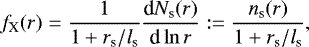 (8)
(8)
where rs is the position of the shock front, and Ns(r) the cumulative number of shocks until radius r. In other words, for a constant number of new, emerging shocks, ns (r) = const., the volume filling factor remains constant only if ls ≫ rs, that is, for adiabatic cooling16. Consequently, the X-ray emissivity, ηx(r) ∝ fX ρ2, depends on ρ2, due to the cooling function alone. On the other hand, for ls < rs, in the radiative regime, fX ∝ ns(r)ls∕rs ∝ ns(r)∕(ρrs), such that the effective emissivity depends linearly on ρ.
Although derived in a physically strict way by Ow13, the radiative limit of Eq. (8) can be simply explained as follows: The total volume Vs of an X-rayemitting ensemble of radiative shocks, each with cooling length ls < Δr, and located inside a shell of volume V = 4πr2Δr, can be estimated as
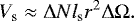 (9)
(9)
Here, ΔN = Ns(r + Δr) − Ns(r) is the number of shocks in between r and r + Δr, and ΔΩ is the solid angle subtended by one shock, for simplicity assumed to be equal for all shocks inside Δr. The effective volume filling factor is then
 (10)
(10)
This is the radiative limit of Eq. (8), corresponding to shocks with a comparatively small cooling length, due to a large density, and proportional to both the shock distribution and ρ−1. Now, if (in the outer wind, or generally for winds of low density) the density becomes as low as to result in ls ≥ rs, adiabatic cooling takes over, and the radiative cooling length does no longer play any role. Then (for details, see Ow13), the volume filling factor becomes solely controlled by the shock distribution, and the emissivity depends on ρ2.
Thus, it is basically the assumption of a spatially constant volume filling factor (as adopted in Carneiro et al. 2016) that differs from the result by Ow13 on fX, and it is easy to unify both approaches. At first, we checked that the (radiative) cooling lengths as quantified by Feldmeier et al. (1997) (and used by FASTWIND) and by Ow13 are consistent: indeed, the basic dependencies
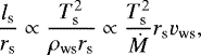 (11)
(11)
with ρws and vws the wind density and wind velocity at the shock front, respectively, and adopting a cooling function ∝ T−1∕2 in the relevant temperaturerange (for example, Raymond et al. 1976; Schure et al. 2009) – are identical, and only the numerical fore-factors are different, by a factor of three (with ls from Ow13 being the larger one).
In the following simulations, we neglected the potential effects of thin shell mixing (which can be easily included if required), and introduced a new input option, allowing us to replace the previous (spatially constant) volume filling factor by Eq. (8). Again following Ow13, we adopt
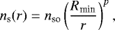 (12)
(12)
where nso and p are additional input parameters, and nso is adapted until a specified Lx value is reached. The input quantity Rmin (denoted as Ro by Ow13) is the onset of shock formation and X-ray emission, typically on the order of 1.5 R* (cf. Carneiro et al. 2016 and references therein), and other input parameters describing the shock temperature just after the discontinuity are used in agreement with the description in Carneiro et al. (2016, Sect. 2.1). Finally, and somewhat inconsistent, we keep our previous method to switch from the radiative to an adiabatic post-shock temperature and density stratification when the cooling and the dynamical wind flow times are identical.
All following simulations have been performed with our new FASTWIND version including complete CMF transfer, and photospheric and wind parameters in most cases similar to those derived for the O4I(f) supergiant ζ Pup, see Table 3. For simplicity, and to allow for an easy comparison with analytical predictions and earlier work, the wind is adopted as smooth, with a mass-loss rate (if not specified differently) that matches the Hα wind emission. This mass-loss rate is a factor of four higher than derived from analyses accounting for optically thin clumping (Najarro et al. 2011; Bouret et al. 2012). CNO abundances have been been taken from Cohen et al. (2010)17, again for consistency with earlier work.
Figure 13 displays the run of the volume filling factor for four different X-ray emission models (see Table 4), using either a constant volume filling factor, fX =const., or a volume filling factor consistent with Ow13, and different shock distributions, with p ∈ [0, 1, 2] according to Eqs. (8) and (12). All values for fX and nso, respectively,have been chosen such that the resulting X-ray luminosity (in the range 0.1–2.5 keV) becomes Lx ∕Lbol = 10−7, a prototypicalvalue for massive O-stars (Chlebowski & Garmany 1991; Sana et al. 2006).
Since, due to the large mass-loss rate, the ratio ls∕rs remains below unity troughout the wind for this specific parameter set, the effective volume filling factor behaves as
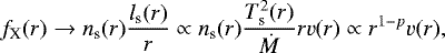 (13)
(13)
which leads, for roughly constant shock temperatures, to a steep increase ∝ rv(r) for p = 0, a moderate increase ∝ v(r) for p = 1, and to increasing and later on decreasing values ∝ v(r)∕r for p = 2, in accordance with Fig. 13.
Stellar, wind, and X-ray emission parameters common to all our ζ Pup-like models.
4.2 Testing predicted scaling relations for the X-ray luminosity
Using our new “unified approach,” we can now re-check the scaling of the X-ray luminosity with wind-density parameter Ṁ ∕v∞, and compare it with the predictions by Ow13. Figure 14 shows the result of such an analysis, where we display our findings when applying the different parameterizations for the effective volume filling factor as introduced above. For all four models series (fX = const., and p ∈ [0, 1, 2], see Table 4), we used the same photospheric and wind parameters as displayed in Table 3, but varied, within each series, the mass-loss rate in the range 10−9−10−4.5 M⊙ yr−1. To allow for a clear comparison, we did not vary the value of v∞, thus in the following we actually check only the reaction of Lx versus Ṁ for the case v∞ = const.
If we denote the typical radius where the wind becomes optically thick in X-rays (due to “cold” material) by R1, and Ra as the border between radiative and adiabatic cooling (in the current framework defined by ls (Ra) = Ra), we can summarize the predictions by Owocki & Cohen (1999) and Ow13 as follows (again discarding potential thin-shell mixing):
I. Optically thin conditions (R1 < Rmin).
a) For a constant volume filling factor, fX = const., or purely adiabatic cooling (Ra < Rmin), the X-ray luminosity should scale as 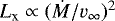 .
.
b) For a volume filling factor according to Eq. (8), and for radiative and adiabatic cooling with Ra > Rmin, a scaling via Lx ∝ (Ṁ∕v∞) is predicted.
II. Optically thick conditions (R1 > Rmin).
a) For a constant volume filling factor, Lx ∝ (Ṁ∕v∞).
b) When fX is defined according to Eq. (8), and for radiative and adiabatic cooling with R1 < Ra, the X-ray luminosity should follow 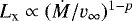 .
.
Comparing these predictions with Fig. 14, we see a fair agreement. For constant volume filling factors (case Ia: “old” approach, green plus signs), there is only the division between optically thin (“slope = 2”) and optically thick (“slope = 1”) conditions, independent of radiative or adiabatic cooling, and in agreement with the former predictions by Owocki & Cohen (1999) and simulations by Carneiro et al. (2016). The transition takes place at the dashed line, which displays the maximum wind density until which the X-ray radiation field remains optically thin in the region above Rmin for all considered frequencies. A “slope = 2” is also present for the other series with fX according to Eq. (8), as long as the wind-density is so low that Ra < Rmin. However, for these models the slope changes toward unity when the wind density increases, even if the wind is still optically thin for X-rays (case Ib). This is particularly visible for the model with p = 2 (red squares).
When the wind becomes optically thick (beginning to the right of the dashed line), the slope changes again. For constant volume filling factors (case IIa), toward a slope of unity, and for the models with varying filling factor, at least in the spirit predicted by case IIb, toward 1 − p. In particular, for p = 2, the slope becomes negative, that is, for increasing mass-loss the X-ray luminosity decreases; for p = 1, the slope becomes (almost) constant; and for p = 0 it remains positive, though flatter than analytically predicted.
The reason for the latter deviation between predicted and simulated slope in the regime to the right of the vertical dashed line is at least two-fold. First, the calculated luminosity is an integral over a large range of frequencies. Whereas to the left of the dividing line, the radiation field is optically thin at all contributing frequencies, it becomes optically thick at all frequencies only for the highest wind-density models considered. In between, the lower energies are optically thick, whereas the higher ones are still optically thin. For example, for log Ṁ∕v∞ = −6.35 in the units of Fig. 14, the radiation field is still optically thin for wavelengths below 15 Å (0.83 keV). Thus, in many cases the luminosity consists of a combination of optically thin and thick radiation, contrasted to the analytic limits. Second, we note that part of the quantitative discrepancies might be caused by numerical issues, related to the less reliable flux determinations in models which are still optically thick at the outer boundary.
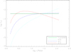 |
Fig. 13 X-ray volume filling factor, fX, as a function of log r∕R*, for different shock distributions parameterized according to Eqs. (8) and (12) (see legend, and Table 4), and stellar and wind parameters for our ζ Pup-like model (Table 3). The vertical dotted line denotes the region where cooling and wind flow times are equal, tc = tf. Due to the large mass-loss rate, the ratio ls∕rs remains smaller than unity throughout the wind. |
Volume filling factors for four different model series.
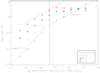 |
Fig. 14 X-ray luminosity (in the range 0.1–2.5 keV, and in units of Lbol) as a functionof Ṁ∕v∞, for stellar models with photospheric and wind parameters as in Table 3, but mass-loss rates ranging in between 10−9 and 10−4.5 M⊙ yr−1, and different assumptions on fX(r) (see legend, and Table 4). The dotted lines display linear relations (with respect to the log–log scaling), with slopes m = 1 and 2, to guide the eye. Models to the left of and at the vertical dashed line are optically thin in the X-ray emitting region at all contributing frequencies, i.e., R1 < Rmin for energies between 0.1 and 2.5 keV. See text. |
4.3 Impact on ionization fractions, and the O VI resonance doublet
To date, it is still unclear which kind of parameterization of the shock distribution is more consistent with real wind conditions. To this end, a careful analysis of UV P Cygni resonance lines (in particular, O VI) might be valuable. Though this is beyond the scope of this paper, we have checked the influence of different fX -stratifications onto the ionization balance, and onto the O VI line profile (see also Carneiro et al. 2016 for the case of fX = const.). In Fig. 15, we display the changes introduced to the ionization fractions of nitrogen and oxygen by X-ray emission, for the same model (similar to ζ Pup) as discussed before, and various fX-stratifications. The results from a corresponding model without any X-ray emission is displayed in black. We concentrate here on nitrogen and oxygen, since, for example, carbon and phosphorus are barely affected in the considered parameter range (see also Carneiro et al. 2016).
Within nitrogen and oxygen, the largest changes occur for N VI and O VI, and are present from the onset of X-ray emission on. On the other hand, N V and O V change only in the outer wind, and the lower ionization stages (III – not displayed, and IV) are not affected at all. Though particularly O VI is increased by many decades for all fX -stratifications considered (explaining the origin of the well-known “super-ionization,” Snow & Morton 1976; Lamers & Morton 1976; Hamann 1980), different shock distributions result in quite different ionization fractions, where, particularly in the lower and intermediate wind, these fractions follow the strength of fX (cf. Fig. 13). Though this behavior should allow for tight constraints when comparing with observations, we note that for such an objective all other parameters need to be known quite precisely, in particular regarding abundances and wind inhomogeneities.
Indeed, when comparing the resulting synthetic O VI-doublets with the corresponding COPERNICUS spectrum for ζ Pup in Fig. 1618, a strong dependence on the adopted wind structure becomes visible. Before commenting on the impact of different shock distributions, we first concentrate on this dependence on wind structure.
As already outlined before, our standard model (Table 3) adopts a mass-loss rate that is a factor of four larger than the observationally derived one when accounting for optically thin clumping. This should certainly affect the profiles: for example, and at least for optically thin clumping, lines with an opacity scaling linearly with ρ, such as C IV λλ1548-1550 (but not O VI), should scale with the “actual” mass-loss rate, (almost) independent of the adopted clumping factor, fcl (for example, Puls 2008 and references therein). On the other hand, and based on analytic considerations, Zsargó et al. (2008) highlighted a completely different relation for those lines where Auger-ionization (due to X-ray emission) dominates, as often (but not always, see Carneiro et al. 2016) the case for the superionized O VI resonance line discussed here. Then, the profiles should become (almost) independent on mass-loss rate for smooth winds, and should depend on the adopted clumping stratification alone if inhomogeneous winds were considered.
To check and demonstrate whether these predictions are followed by FASTWIND, we synthesized the O VI-doublets for our standard model (M1), and three additional ones, with wind-parameters provided in Table 5. For these additional models, we calibrated the fX and nso parameters as to obtain the same X-ray luminosity as present in model M1. Model M2 is still a smooth model, but with a mass-loss rate corresponding to the observationally derived value (a factor of four lower compared to M1). Indeed, and as predicted by Zsargó et al. (2008), the profiles for both smooth-wind models M1 and M2 are very similar, despite the large difference in Ṁ. When subsequently increasing the clumping factor in models M3 and M4 (that is, compressing the wind mass into smaller and smaller clump-volumes), the profile-strengths decrease (again as predicted, because of increased recombination inside the clumps). We note that the M4 profiles differ only weakly from a corresponding model without any X-ray emission at all. When finally comparing our profiles for models M1 and M4 to those resulting from the (CMFGEN incl. X-ray) simulations19 by Zsargó et al. (2008, their Fig. 1), we find an extremely close agreement, also here proving the consistency between FASTWIND and CMFGEN.
Among the displayed models, M4 is the one closest to results from analyses of ζ Pup, performed in the UV (though excluding O VI), optical, NIR, and radio domain, and assuming optically thin clumping (Puls et al. 2006; Najarro et al. 2011; Bouret et al. 2012). From the severe discrepancy between observations and simulations, one might conclude that there is also a severe problem with the inferred parameters. However, Zsargó et al. (2008) have flagged the importance of the inter-clump medium for a correct description of the O VI resonance line formation. They showed thatwhen relaxing the assumption of a void inter-clump medium, and accounting for reasonably low, but non-zero densities in such regions, its contribution is sufficient to explain the observed profile strength. Since corresponding simulations require a two-component, NLTE description, this is beyond the scope of FASTWIND’s current capabilities. Instead, we consider the mass-loss independent, smooth-wind case. For our purposes, this should be close enough to the conditions in an inhomogeneous wind, when a low-density inter-clump medium covers a large volume, and the contribution from the overdense region is negligible. In particular, and to investigate the dependence on different shock-distributions, in the following we concentrate on the profiles for models M1 or M2.
Without any X-rays (black), there is no signal at all, whereas for all simulations including X-rays, a P Cygni profile is clearly visible. Since the absorption troughs are not saturated, the absorption strength is proportional to the ionization fraction, and hence to the run of fX (see above). We note that corresponding normalization factors are well-constrained, since the adopted X-ray luminosity is close to the observed one for ζ Pup, log (Lx∕Lbol) ≈−7.15 to −6.85 (Berghoefer et al. 1996; Pauldrach et al. 2001; Zsargó et al. 2008). For the considered models, a constant volume filling factor, or a filling factor that is rather similar (here: p = 2), result in profiles that are closest to observations. In all cases, however, the line emission from the lower wind is too large, and/or the absorption is too low, which might be cured by a combination of a lower Rmin value and modified X-ray filling factors in those regions, and, ultimately, by an appropriate clumping law including a consistent description of the interclump medium. From the absorption strength at high velocities (where all fX values are similar), it might be concluded that both our description and the used abundances are reasonable. And indeed, the oxygen abundance adopted in our X-ray emitting models,  = 0.2, is close to the value derived by Bouret et al. 2012,
  = 0.25.
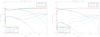 |
Fig. 15 Ionization fractions of nitrogen and oxygen, as a function of v(r)∕v∞, for the samestellar model and shock distributions as in Fig. 13. For line-coding, see legends. |
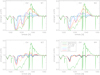 |
Fig. 16 Synthetic line profiles for the UV resonance doublet of O VI, for the same stellar model and different shock distributions as in Fig. 13 (M1, upper left), and for three other models (M2 to M4) differing in mass-loss rate and clumping properties (see Table. 5). Same color coding as in Fig. 15. Profiles from the smooth-wind models M1 and M2 are close to being identical, though mass-loss rates differ by a factorof four. All spectra have been calculated with a depth dependent “micro-turbulence” (proportional to v(r), with a minimum of 15 km s−1, and a maximum of 0.1v∞), and convolved with v sin i = 220 km s−1. For comparison, the observed COPERNICUS spectrum (at a resolution of 0.2 Å, Snow & Jenkins 1977) is displayed in dark green. The dotted lines at the top display the rest-frame frequencies of the doublet components. The absorption feature around 1215 Å, visible in all synthetic spectra without significant O VI contribution, is stellar Lyβ. Model M1 and M4 and corresponding spectra (for fX = const.) are very similar to those displayed (and discussed) by Zsargó et al. (2008) in their Fig. 1. |
5 Summary and conclusions
The work presented in the previous sections can be summarized as follows: we have updated our unified, NLTE atmosphere and spectrum synthesis code, FASTWIND v10, by including – via a new program module – a detailed comoving frame transfer covering the most important wavelength range (current default: from 200 to 10 000 Å, where these limits can be modified by the user). The new version is called FASTWIND v11. Both explicit and the most important background elements (called selected) are handled with similarly high precision, and only the non-selected elements are treated within our previous, approximate NLTE approach, though also here the required radiation field is taken from the detailed (though re-mapped) CMF solution. In the default version, both the ray-by-ray solution for the specific intensity, and the moments equations are solved subsequently.
The major part of computation time is spent by the ray-by-ray solution, which mostly depends on the adopted micro-turbulent velocity, vmic. Total turnaround times including the final observer’s frame formal integral to calculate emergent fluxes and normalized spectra, are on the order of 1.3 to 1.9 h for vmic = 15 km s−1, and 3 to 4.5 h for vmic = 5 km s−1, for an Intel Xeon 2.7 GHz processor, where the lower values refer to models with H and He as explicit elements (fast convergence), and the higher values to a combination of explicit elements that is slowly converging, due to complex line-overlap processes (for example, H, He, N). The required RAM amounts to a comparatively low value of 1.6 GB.
We have carefully compared our results with alternative ones from CMFGEN and our previous version, FASTWIND v10, by means of a comprehensive model grid covering early B- to hot O-type dwarfs and supergiants. We confirm previous results on the deviations between an exact and the approximate NLTE treatment following Puls et al. (2005), which amount, on average, in between few to 20% for the main ionization fractions, though with a significant scatter.
The total radiative acceleration as calculated by CMFGEN and FASTWIND v11 agrees almost perfectly for the supergiant models, whereas for dwarf models there is a certain discrepancy in the transonic region, presumably related to different velocity fields in thisregime, and to different line-lists. The overall remarkable agreement (already mentioned in a first announcement of v11, Puls 2017) justifies its usage within the calculation of self-consistent wind models, as performed by Sundqvist et al. (2019). In particular, the strong decrease in the acceleration in the transonic region, predicted by both CMFGEN and FASTWIND for late O-dwarf models (here: d10v), might be responsible (at least in part) for the weak-wind effect in cooler dwarfs (lower observed mass-loss rates than resulting from “simplified” theories, for example Puls 2008 and references therein). This conjecture is corroborated from corresponding results from the self-consistent wind models quoted just above.
Also the optical H and He spectra agree in most cases very well, and only for He II λλ4200-4541 there are, similar as for FASTWIND v10, certain differences in the line-cores. Morever, and most promising, we find the same He I problem as identified by Najarro (2006), and have patched it in a similar way. The agreement between the old and the new FASTWIND is even better, and an analysis with both codes should result in parameters which are close to being identical. This finding allows, for example, for still using the older v10 approach whenever a pure HHe analysis in the optical is sufficient, by simply switching back to this version via the corresponding option inside the code (see Sect. 2.1).
With respect to diagnostic nitrogen line profiles in the optical, the agreement is still acceptable, though for specific transitions the differences are no longer insignificant. The largest difference occurs for N V λλ4603-4619 (when present), where our new version predicts stronger absorption.
We have re-investigated the formation of N III λλ4634− 4640−4642, and confirmed the basic findings by Rivero González et al. (2011). In particular, the agreement with CMFGEN could be improved, because the shortcomings of the previous v10 (neglect of line-overlap effects) are no longer present in v11. However, we have also identified one additional, Fe V line in the EUV, which participates in the formation of the N III emission lines. In combination with the adopted size of vmic, and in dependence of Fe, O, and N abundances, the emission strengths of these lines can become quite non-monotonic.
Overall, we warned the reader against uncritically relying on the He I singlets, the N III emission lines, and N V λλ4603–4619, when performing quantitative H-He-N spectroscopy in the optical, and to put a lower weight onto these lines, compared to others. The impact of vmic (allowing or prohibiting specific line-overlaps) needs to be always kept in mind.
With the new FASTWIND version, we are now able to synthesize large continuous portions of the spectrum, in particular the UV range. Also here, the agreement with CMFGEN is mostly excellent, and the only relevant differences concern the sulfur (resonance) lines (future checks required!), and the pseudo-continuum of the coolest models within our grid, which in the CMFGEN models is considerably more depressed. This depression (particularly around Lyα) is almost exclusively due to Fe IV lines connecting energy levels that are not observationally confirmed. Indeed, when comparing with observations, many of these lines seem to be absent, and one of the future tasks is to carefully check this issue, which certainly is not only an “academic” one. (i) As extensively discussed in the previous sections, line-overlap in the EUV (particularly with Fe lines) can significantly affect the population of various levels, and thus the absorption and emissions strengths of diagnostic lines. Hence, it is of prime importance to check whether such Fe-lines are actually present, or not. (ii) When investigating the UV spectrum of fast rotators, the definition of a reliable continuum level becomes problematic, if the line density was indeed as high as predicted by current models. In this case, normalization procedures might result, in specific wavelength regimes, in an erroneous continuum level (Fig. 12, upper panel, and particularly the predicted flux distribution for model s10a, Fig. 11), which in turn might lead to erroneous conclusions when comparing with theoretical models that do not include a consistent metallic background. (iii) If, on the other hand, Fe IV lines play a lesser role in specific models compared to others (as here for the case FASTWIND versus CMFGEN), the pseudo-continuum is closer to unity, and the emission peaks of P Cygni lines appear higher in a normalized spectrum. Thus, the reliability of the Fe IV background can directly affect the wind diagnostics. Obviously, not only Fe IV, but also lower ionization stages (Fe III and Fe II in B- and A-type supergiants) need to be investigated as well.
In the last section of this work, we unified the seemingly discordant results on the X-ray emission from wind-embedded shocks when using the models by either Feldmeier et al. (1997) or Owocki et al. (2013). As it turned out, the assumption of a depth-independent X-ray filling factor, when combined with the former approach, is the origin of this discordance. By alternatively applying the depth-dependent expression provided by Owocki et al. (2013), both approaches could be unified. Scaling relations for the X-ray luminosity as a function of wind density, as calculated by our new FASTWIND version, agree well with the analytical expression provided by Owocki et al. (2013). A first comparison of the super-ionized O VI resonance line in the UV with observations indicated that this line is well suited to obtain clues on the shock distribution, but only if a meaningfull description of the inter-clump medium has become available.
Aside from a solution of the problems discussed throughout this paper, the next steps in our further program development are obvious. On the programing side, we might think about parallelization. This should be possible for the most time-consuming part, the ray-by-ray solution, when the outermost loop extends over p-rays instead of over wavelengths. Such a modification would increase the required memory, and it might be better to keep our present strategy of calculating different models in parallel, which is suitable at least for the construction of model grids. When applying on-the-fly optimization strategies such as genetic algorithms, a shorter wall-clock time due to parallelization might be advantageous though.
Regarding future updates of the involved physics, a rather simple improvement concerns the implementation of optically thick wind clumping, which was already done in FASTWIND v10 (Sundqvist & Puls 2018), and needs only to be included into the new routines of v11 (and tested!). Most importantly, however, is an improvement of our Fe (and Ni) model atoms, to include higher lying levels into the detailed NLTE treatment. To date, it is not clear whether we can continue with our current approach of packing suitable levels, or whether we will completely switch to a more general super-level approach for these elements. Finally, it will be of highest relevance to extend our presently considered wavelength range into the NIR, to be prepared for the upcoming observations of next-generation telescopes.
Acknowledgements
We gratefully thank our anonymous referee for very constructive comments and suggestions. Particular thanks to the late Adi Pauldrach for providing us with the WM-BASIC data base, and to John Hillier for making CMFGEN available. F.N. acknowledges financial support through Spanish grant ESP2017-86582-C4-1-R (MINECO/FEDER) and from the Spanish State Research Agency (AEI) through the Unidad de Excelencia “María de Maeztu”–Centro de Astrobiología (CSIC-INTA) project No. MDM-2017-0737. J.O.S. acknowledges support by the Belgian Research Foundation Flanders (FWO) Odysseus program under grant number G0H9218N, as well as from the KU Leuven C1 grant MAESTRO C16/17/007. K.S. would like to thank the DAAD (WISE) Scholarship and Inspire Fellowship (DST) programs for financial support, and colleagues at the USM Munich for hosting during an internship. This paper is dedicated to Adi Pauldrach, who left us much too early. We will always remember his personality, his laughter, his dedication to soccer, and his invaluable contributions with respect to line-driven winds, NLTE-modeling of massive star atmospheres, and manifold applications. May he rest in peace.
Appendix A Approximation of the incident intensity required for the CMF transport
In this appendix, we describe our approximation for the incident intensity, I−, at Rmax, the outer boundary of our computational domain (≈120 R*). As already mentioned in Sect. 2.2, and to minimize the computational effort, we do not “extend” the atmosphere in the ray-by-ray solution toward larger radii, as suggested by Hillier & Miller (1998). The latter procedure avoids the specification of a non-zero incident intensity, I− (Rmax), which otherwise would need to be accounted for, as long as the outer atmosphere is not completely optically thin (and which is difficult to estimate). Indeed, a reasonable choice of I− ≠ 0 is often essential for a reliable radiative transfer solution (and related quantities such as occupation numbers) when the outer boundary is not extended beyond the actual grid.
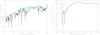 |
Fig. A.1 CMF mean intensity at Rmax (≈ 120 R*), for a hot dwarf model with Teff = 55 000 kK and a large mass-loss rate, calculated with different approximations for the incident intensity, I−, and different wavelength regimes. All intensities have been taken from the same iteration step, namely the first step after the detailed CMF-treatment has been initiated. Color-coding – black: complete incident intensity including frequency derivative, as described in the text; red: I− = 0; dark blue (mostly blended by turquoise): I− specified only for lines and continua of significant optical depth, gradient neglected; turquoise: I− specified for all frequencies, but gradient neglected; green: approximate pseudo-continuum, as used in the previous FASTWIND version, and still at highest and lowest wavelengths. Left panel: EUV range between 200 and 300 Å; right panel: frequency range around the C IV resonance doublet in the UV. |
Instead of such an extension (to reach optically thin conditions and then set I− = 0), we developed and tested an approximate description of I− (Rmax), and its frequency derivative. Also the latter needs to be specified in the CMF equations, because of the presence of the term ∂v∕∂x = ∂u∕∂x − ∂I−∕∂x at the outer boundary, with Feautrier variables u and v, and x the CMF-frequency in suitable units. For example, and as also done in the following, one might define x (in the neighborhood of a line with transition frequency ν0) as a CMF frequency displacement, measured in units of maximum Dopplershift,
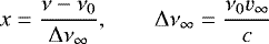 (A.1)
(A.1)
(for the general background and further details on CMF transfer, we refer to Mihalas 1978 and Hubeny & Mihalas 2014).
If, on the other hand, an appropriate incident intensity would be neglected at all, particularly the line cores would become too deep (cf. Fig. A.1, red versus black), and optically thick continua too weak. Our development of an appropriate boundary condition required a number of subsequent steps, which are summarized in the following, and which are (partly) displayed in Figs. A.1 and A.2.
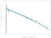 |
Fig. A.2 As Fig. A.1, but for λ = 1500−11 000 Å. The impact of the frequency derivative (turquoise versus black) is clearly visible. Without inclusion, no smooth transition between detailed and approximate treatment (at λmax = 10 000 Å) would be possible. Setting I− to zero at all frequencies (red curve in Fig. A.1) results in a flux-distribution identical to the black one in the optical range, whereas specifying I− ≠ 0 only for optically thick lines and continua, and neglecting the frequency gradient (dark blue curve in Fig. A.1), results in fluxes similar to the turquoise ones. |
Optically thick continuum
By using the (static) equation of transfer (accounting for the fact that in most cases the frequency shift between outermost grid-point and infinity is negligible), the incident intensity can be approximated (to zeroth order in source function, and assuming I− (ν, z →∞, p) = 0) by
 (A.2)
(A.2)
with CMF-frequency ν, and continuum source function and optical depth, Sc and τc, respectively, where τc can be approximated by (analytically) extrapolating the opacities from Rmax to infinity.
Optically thick line cores
Here we use a Sobolev-like approach (following Lucy 1971; Puls 1991), namely neglecting the spatial derivatives in the CMF equation of transfer, and assuming that one line dominates the opacity and source function (a generalization to more than one line is possible, and implemented into our code). This results (see also Puls 2020) in
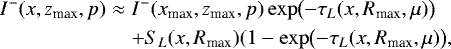 (A.3)
(A.3)
with line source function SL, and line optical depth
 (A.4)
(A.4)
τS is the well-known Sobolev optical depth (depending on line opacity, transition frequency, radial and tangential velocity gradient, and cosine of angle between z- and radial direction, μ = z∕r), and ϕ(x) the appropriate, normalized profile function. Finally, xmax = nmaxvDop∕v∞ denotes the frequency shift at the blue wing of the transition, with nmax ≈ 3−5, in dependence of line-strength, and vDop is the effective Doppler speed, comprising the thermal and the micro-turbulent contribution. As long as there is no close (blueward) line, the first term in Eq. (A.3) can be neglected compared to the second, local one.
Both approximations as outlined above (for optically thick continua and/or lines) can be united, by basically summing up the optical depths, and calculating a total source function (details are beyond the scope of this appendix).
The impact of including this approximate incident intensity can be seen by comparing the line-cores with and without this term (still neglecting its frequency derivative) in Fig. A.1, where the red (I− = 0) and dark blue (coinciding with the turquoise) graphs display the resulting CMF mean intensities evaluated at Rmax. Without I−, the line cores become too deep, while including I− as specified above cures this problem (independent of the specific atmospheric model considered).
Optically thin conditions
If, however, only these terms were accounted for (and even if accounting also for their frequency derivatives), certain atmospheric models might display a problem. This is exemplarily shown in Fig. A.2, for the case of a hot atmosphere with Teff = 55 000 K, and a large mass-loss rate: longward from the “last” strong UV resonance line (C IV), when all lines and the continuum have become optically thin at the outer boundary, the CMF mean intensity begins to deviate from our previous, pseudo-continuum approach (in green, see Sect. 2.1), and this trend continues until the upper limit of our detailed CMF treatment is reached, at λmax = 10 000 Å. One might argue that our new solution is simply more accurate than the previous one, because of the inherentapproximations within the latter. However, (i), our previous approach has been carefully tested, by comparing the results for large model grids with corresponding CMFGEN and WM-BASIC solutions, and particularly the optical flux distributions turned out to be very similar (see Puls et al. 2005, their Figs. 8 and 15). After all, those fluxes are dominated by electron-scattering, and by bound-free and free–free opacities and emissivities from H and He, which are not affected from our opacity sampling approach in v10. (ii) Test-calculations using v11 with I− = 0 at all frequencies resulted in optical fluxes almost identical to those from v10. Thus, there is a problem, and one might speculate whether this problem is related to processes neglected thus far.
Indeed, and after many tests, it turned out that the discrepancy is due to large inward directed intensities at high impact parameters (p → Rmax, μ → 0) arising within the solution for the last strong line. These intensities did not “decay” when proceeding toward longer wavelengths in the CMF transport, resulting in overestimated mean intensities close to the outer boundary, and contaminating the solution throughout the complete optical range. The reason for these large intensities relates to the large value of I− at the red end of the last optically thick line core. Without appropriate means, this large value cannot decrease within the frequency transport, as long as the opacities are low (cf. Eq. (A.3), first term), which is often true for the considered outer region and directions.
In reality, however, there is a decay, due to the fact that, for wavelengths redward from the last line core, the illumination from above is controlled by resonance zones that move outward as the wavelengths increase, into the region outside the computational domain, far beyond zmax (the extended region in CMFGEN). Consequently, I− decreases from its maximum value (at the red edge of the last optically thick line core) to zero, and this decrease, in combination with the corresponding frequency derivative, leads to an effective negative source term at the outer boundary, enabling more realistic solutions (black versus dark blue and turquoise in Fig. A.2).
Thus, at first we have to define the frequency range over which I− declines to zero (when the resonance zone has reached “infinity”), from its starting value  , where “red” should denote the red edge of the previous line core, x = xred = −xmax. Without any (continuum) absorption and emission, the specific intensities remain constant along the characteristics of the partial differential equations decribing the CMF transfer, and for inward directed radiation, this leads to (for example Puls 2020)
 (A.5)
(A.5)
At the outer boundary, v(r)∕v∞ is close to unity. Thus, for “core rays” with p ≤ R* and μ(zmax) → 1, Δx is small, since the outermost resonance zone which can give rise to a non-zero incident intensity must fulfill the condition μv(r)∕v∞ + Δx = 1 − ɛ + Δx := 1 (in the limit of negligible thermal+micro-turbulent speeds, and with ɛ a small number). However, for large impact parameters (which had been identified as the “problematic” rays), μ is quite low, and we find that
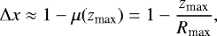 (A.6)
(A.6)
which is on the order of unity, and thus corresponds to dozens to hundreds of thermal (including micro-turbulence) Doppler shifts.
Summarizing, for x-values20 close to the red edge of the previous line core, the outer boundary is illuminated by an intensity close to  , whereas for frequencies lower than x = xred − Δx, there is no longer any resonance zone which could illuminate the outer boundary at x, and I− (x) must be zero (if the continuum is optically thin).
To simplify our solution scheme, we assume that I−(x) decreases linearly from  at x = xred to zero at x = xred − Δx, with Δx from Eq. (A.6), which allows us to specify both I−(x),
![Mathematical equation: \begin{equation*}I^-(x) \approx I^-_{\textrm{red}} \left(1 - \frac{x_{\textrm{red}} - x}{\Delta x}\right), \quad x \in [x_{\textrm{red}}, x_{\textrm{red}}-\Delta x], \end{equation*}](/articles/aa/full_html/2020/10/aa38464-20/aa38464-20-eq33.png) (A.7)
(A.7)
and its frequency derivative in an easy and computationally fast way. As argued above, the corresponding terms are (almost) irrelevant for core-rays, but for rays with large impact parameter, which moreover have a large weight for the mean intensity, they are significant, and lead, overall, to a perfect representation of the run of Jν (Rmax) (black versus green relations in Fig. A.2). We note that it is indeed the gradient of I− which is the decisive component: using the I− term as estimated above alone (turquoise relation) does not mitigate the problem.
Under certain conditions, the continuum might be optically thick at x = xred. Then, the same strategy as above might be applied, but xred replaced by the frequency where the continuum becomes optically thin, and  replaced by the corresponding quantity using Eq. (A.2) (or an appropriate combination with overlapping line processes).
Line overlap effects
A final complication might arise because of strong lines seperated by less than Δx = 1, as present, for example, for most UV resonance doublets. In this case, the incident intensity for the red component needs to be modified, due to the direct illumination by the blue one, which corresponds to a non-negligible first term in Eq. (A.3). There are certainly better approximations, but in our current approach we simply use the maximum of I− (x), either calculated from Eq. (A.7), with  derived at the red edge of the blue component, or from the local term proportional to the source function in Eq. (A.3)21. This approach has not led to any obvious problems to date.
Collecting all our findings, there are two basic possibilities to deal with I− (x, zmax, p). Either, one adopts I− = 0 at all frequency points, and accepts certain inconsistencies in the line cores and optically thick continua; or one has to provide an adequate I−≠0 including its frequency derivative, even for optically thin conditions, at least within the range xred…xred − 1 to the red of all optically thick line cores. Both formulations ensure that the detailed CMF solution and the pseudo-continuum treatment are consistent within the optical regime, and particularly at λmax. However, only a physically correct prescription with I−≠0 allows for a similar consistency around λmin, since in thelatter regime the continuum is often optically thick beyond Rmax, and many optically thick lines are present as well. Moreover, if one aims at a solution of the CMF transfer using the moments equations, the second method, exclusively used in our current FASTWIND version, is certainly better suited, since otherwise the required ratios of intensity moments often display an abrupt change at the outer boundary, giving rise to numerical artifacts.
Appendix B Convergence behavior
The convergence behavior for various set-ups offered by our implementation is displayed in Fig. B.1. In particular, we compare our default procedure (ray-by-ray solution plus moments equations, black) with an approach using the ray-by-ray solution alone. The impact of different sets of explicit elements is also compared. In the former approach, we used H, He, and N, as explict elements22, whereas in the latter, we either considered the same elements (red), or H and He only (blue).
Figure B.1 allows us both to explain our basic strategy, and to discuss two prototypical situations with respect to convergence behavior. In all panels, we display the maximum (regarding all grid-points) relative change of temperature (dashed) within two consecutive iteration steps, and the corresponding radial mean of the maximum change within all specified (cf. Sect. 2.2) occupation numbers. In the latter case, we provide the (radial) mean, to suppress local maxima which sometimes occur, but we average the maxima per grid point only over the most important region with τRoss ≤ 1, since for larger optical depths the occupation numbers begin to thermalize, and corresponding changes become very low (typically, on the order of 10−4 to −5). If included into the averaging, this region would bias the result.
Before concentrating on the convergence properties, we explain our basic strategy, by means of the upper panels corresponding to our hottest dwarf model (d2v), with parameters provided in Table 2. The left and right panels display the changes within the explicit and the selected background elements.
During the first 30 iterations, we follow our previous FASTWIND version, namely performing 10 to 20 iterations with Sobolev line transferfor all elements, and then switching to the CMF approach for the explicit and most important background transitions, using in parallel the pseudo-continuum approach. As displayed, the convergence is very fast, both for occupation numbers and temperature. If we would continue with this approach, as done in FASTWIND v10, the complete model would have converged after a total of 40 to 60 iterations. In the new version, however, we switch to the detailed CMF calculations (in between λmin and λmax), at iteration #30, indicated by the dotted vertical line. Immediately, the occupation numbers and the temperature structure change significantly,not the least because the Rosseland optical depths change at each grid point (detailed calculation versus sampling), though typically by only few percent. After a while, the temperature begins to stabilize again, and we perform an update of the photospheric structure (particularly accounting for the updated radiative acceleration), indicated by the dashed vertical line. As already explained in Rivero González et al. (2012a), one such update is usually sufficient, as long as it is performed not too early. From this point on, the temperature stabilizes again, and we consider it as converged, if the maximum changes are below 0.3% (indicated by the dotted horizontal line). Ideally, one would iterate the temperature and occupation numbers in parallel, until a final, common convergence has been reached (as done in models employing a complete linearization). In our method, however, even small changes in temperature directly couple to changes in occupation numbers. Consequently, we would need a much larger number of iterations until the convergence criterion has been reached, though the final changes in temperature (compared to our standard treatment) would be marginal. Indeed, after the temperature has been considered as converged and remains fixed, also the occupation numbers stabilize (for the inspected model, quite quickly), and we consider the model as converged when the mean maximum changes fall below 10−3 to 10−4. Moreover, in each iteration we check the flux-conservation. For all models computed thus far, this condition remains fulfilled (typically at the one to two percent level) also after temperature convergence, that is, after the temperature has been fixed, and only the occupation numbers are allowed to vary.
To increase the final convergence, we apply a Ng-extrapolation (Ng 1974) for the source functions of important resonance lines (here: from C, N, O); extrapolating the source functions from all line transitions is computationally prohibitive, since, to perform such an extrapolation, the values from at least three prior iteration steps would need to be stored.
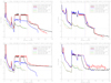 |
Fig. B.1 Prototypical convergence behavior for three different kinds of model calculations (see legend and text). Displayed is the maximum relative change of temperature (regarding all grid-points, dashed) within two consecutive iteration steps, and the corresponding mean of the maximum change within all specified occupation numbers, where the averaging has been performed over all depth-points with τRoss ≤ 1. Left panels: mean maximum change within occupation numbers from explicit elements (HHeN in black and red, HHe in blue); right panels: mean maximum change within occupation numbers from selected background elements. Upper and lower panels: convergence behavior for our hottest dwarf (d2v, see Table 2) and supergiant (s2a) model, respectively. Our convergence criterion for the temperature is displayed by a horizontal dotted line. The vertical lines display the onset of the detailed CMF calculations within λmin and λmax (dotted), the update of the photospheric structure (dashed), and the onset of the Ng-extrapolation scheme for the C, N, O resonancelines (dashed-dotted). See text. |
At first we note that, for all three set-ups, the temperature convergence is very similar, which is also true for the occupation numbers from the selected elements. For the explicit elements, on the other hand, the mean maximum deviations for the HHeN models are larger than for the HHe model, which indicates that the convergence of nitrogen is more problematic than that of H and He, at least when a detailed atomic model is used, and all levels are inspected for convergence. Nevertheless, for this hot dwarf model, the occupation numbers from all elements eventually converge.
This is no longer true for the second model displayed in the lower panels, a model for a hot supergiant (s2a). Here, a well-behaved convergence is present only for the model with HHe as explicit elements (in blue). Interestingly, the selected elements, in particular, N, seem to show a better final convergence, compared to the case when N is treated as an explicit element (left lower panel, in red). However, this is mostly due to our recipe for evaluating the maximum changes. As explained in Sect. 2.2, for explicit elements we inspect all levels, because of our requirement for high precision. For selected elements, we only account for changes in the ionization fractions though. Since the convergence problems (see below) mostly concern the excited levels of N (connecting the triplet lines around 4640 Å), these problems do not show up in the displayed maximum changes. Thus, N (selected), in concert with the other selected elements, seems to converge without problems, contrasted to the case when N has been treated as an explicit element.
On the other hand, both models with HHeN (in black and red) display an oscillatory behavior (with respect to maximum changes) in the last iterations, close to the one-percent level. Before providing further details, we note that also here the temperaturehas converged after roughly 60 iterations, which is also true for the other models discussed in the current study (Sect. 3), except for model s8a. Independent from set-up, the latter requires roughly 110 iterations to achieve a converged temperature structure; interestingly, the corresponding CMFGEN model has similar difficulties, which indicates that it is located in a parameter regime where specific processes can easily push the ionization equilibrium and/or optical depths into different directions.
The origin of the apparently bad convergence of the occupation numbers is mostly related to line-overlap effects (in rest-frame, or wind-induced), particularly between strong lines of C, N, O, and Fe (either between different elements, or between different ions of the same element, Rivero González et al. 2011; Martins & Hillier 2012), discussed in more detail in Sect. 3. In those cases where one of the overlapping lines strongly dominates, the overlap does not lead to specific problems (in this case, the source function of the weaker component will adapt to the source function of the stronger one). If, however, both lines have a similar strength, an oscillatory behavior becomes possible, as visible for model s2a (both in the explicit and selected elements, which are coupled via such line overlap effects). Until to-date, we found no real means to improve the situation, that is, to ensure convergence for all levels at all depth-points. Moreover, analytic considerations based on simplified but similar conditions indicated that such oscillations are possible indeed, independent of the specific iteration scheme. Thus, we investigated how the occupation numbers and the synthetic spectrum are affected by different start models, different extrapolation schemes, different damping procedures, and so on. As a major conclusion, we found that a large number of iterations (on the order of 140, as displayed in Fig. B.1) is usually sufficient to obtain a more or less unique solution, with only few oscillating levels over a restricted spatial domain. In this case, the emergent spectra become very similar for the various test models (with maximum differences on the order of few percent in the peak heights or depths of few lines), independent of convergence history: due to the oscillatory behavior of the affected levels, there is only a limited range over which they vary, and most other levels can and indeed do converge. Additionally, the oscillation pattern, if present, often occurs only inside the intermediate wind, above 0.1 v∞, such that photospheric profiles, even if in emission due to NLTE effects, are not affected at all.
Appendix C More technical issues
C.1 Re-mapping of radiation field, and non-coherent electron scattering
To save computational time, we re-map the mean intensities resulting from our detailed CMF calculations (with Nf frequency points, see Eq. (4)) onto a coarser grid, which in the very first iteration steps serves as a frequency grid for the continuum and pseudo-continuum transport. Depending on considered elements (ionization edges to be resolved), this grid comprises between 1000 and 2000 frequency points. The re-mapping is done in such a way that the frequency integral of the mean intensity between two coarse mesh points, νi, νi+1, remains conserved, such that 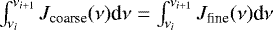 . The re-mapped mean intensities are used to calculate corresponding integrals for the ionization and recombination rates (see also Hillier & Miller 1998; Pauldrach et al. 2001; Rivero González et al. 2011 for the specific case of dielectronic recombination), and for the heating and cooling rates within the electron thermal balance (Kubát et al. 1999). They also enter the Sobolev line-rates for those lines with no information on the upper level (see Appendix C.2) from the selected background elements, as well as the approximate NLTE calculations for the non-selected background. In both latter cases, such rather smooth mean intensities should be used to avoid contamination by narrow features within the detailed solution. Since particularly the ionization and recombination integrals need to be evaluated during each iteration step, and extend over a significant frequency range, the calculation via re-mapped mean intensities is computationally favorable, and introduces only small errors, because of their specific conservation properties.
In contrast, all scattering integrals, ALOs, and total line acceleration are calculated by integrating over the highly resolved CMF frequency grid, where the line acceleration is amended by results for the “outer” ranges below and above the CMF regime (outside λmin–λmax), via corresponding integrals over the approximate pseudo-continuum fluxes.
A second set of mean intensities is additionally calculated, to be used when setting up the (non-coherent) electron scattering emissivities. We note that using coherent scattering instead would induce erroneous results within the line-cores, because of the large electron thermal speeds, giving rise to a frequency redistribution within a range of several thousand km s−1. For the sake of simplicity and computational performance, the corresponding terms are approximated via convolving the CMF mean intensities by electron thermal broadening. This procedure is at least qualitatively similar to results when using the exact redistribution function as provided by Hummer & Mihalas (1967, see also Rybicki & Hummer 1994).
C.2 Total line list, and treatment of lines without information on the upper level.
Since for the explicit elements we use a flexible, DETAIL- (Butler & Giddings 1985) like input for atomic models and transitions, while for the background elements we rely on the fixed-format, WM-BASIC (Pauldrach et al. 2001) data base, we need to adapt our total line list, to be used both in the CMF-transfer and in the final formal integral (see below). The original line list, comprising roughly 2 million entries, is also taken from the WM-BASIC data base, whereas all transitions refering to explicit elements arereplaced (at the begin of the CMF-treatment) by corresponding ones from the DETAIL-input. Because a number of transitions from the latter are packed (for example, those for the N V UV-resonance doublet), they need to be de-packed within the line-list, which is done via one additional data-file (LINES.dat) containing all necessary information23.
Whereas all transitions of the explicit elements have lower and upper levels that are treated within our NLTE network, the line list for the background elements also comprises numerous transitions (mostly from Fe and Ni) where only the lower level is included into the corresponding NLTE rate equations. Indeed, within the background elements, there are roughly “only” 40 000 transitions where also the upper level is explicitly considered. This, because the energy cut-off for the corresponding atomic models has been chosen in such a way as to allow for a numerically stable solution of the linear rate equation system. For calculating the line-blocked radiation field, and also the radiative acceleration, however, also the multitude of lines that have a level beyond this cut-off need to be accounted for. For all such lines (again: this only affects the background elements), we use a two-level, Sobolev approach to estimate the corresponding source functions. Here, the radiative rates are derived by considering the re-mapped CMF mean intensities, and the collisional de-excitation rate coefficients are either estimated from the van Regemorter (1962) approximation for radiatively allowed transitions, or following the semi-empirical expression by Allen (1973, with collision strength Ω =1) for the forbidden ones. The source functions estimated in this way are then used within the subsequent CMF-transfer, such that also these lines participate in the overall iteration scheme.
Since such a two-level approach is justified only for strong transitions connected to the ground or a meta-stable state, it needs to be checked whether this approximation might also be used for excited lower levels, as done per default in our current implementation. A corresponding test has been performed by using an alternative approach, namely by estimating the source-function from an approximate occupation number of the (missing) upper level. This occupation number (actually, divided by its statistical weight) was estimated from its LTE-value (which can be calculated, since the energy of the lower level, and the transition energy is known), times a NLTE departure coefficient. As a crude approximation, the latter was assumed to be identical to the departure coefficient of the highest-lying level (of the considered ion) that is explicitly calculated, and which is connected to the same lower state. Indeed, when comparing models obtained with either approximation (two-level atom, or NLTE with approximate departure coefficient for transitions with “unknown” upper level, and a lower one that is not the ground or a meta-stable state), it turned out that basically all results remain unaffected, for all models within our complete grid (Table 2).
Though our two-level approach yields overall reasonable results, there is one additional problem, which might introduce considerable errors into important diagnostic lines. Namely, since there are numerous lines treated in the above approximation (in particular, from Fe and Ni), there is quite a chance of a coincidental line-overlap with lines that are treated exactly. If, on the one side, the “approximate” line is stronger, the exact line can adapt to source-function equality, since its upper level participates in the NLTE network. In this situation, the final result is reasonable, and nothing needs to be done. If, on the other side, the exact line is dominating, the approximate one should develop a similar source-function as the exact one. This cannot happen though, since the run of its source function depends, via the two-level Sobolev approach, mainly on the escape probabilities, which are barely affected by the exact line. And, since it is not adapting, it might strongly influence the radiation field and thus the source function of the exact line in an erroneous way, at least if its opacity is not too low. An example for this situation is given by the (strategic) N IV 6380 line (see Fig. C.1), with a lower level radiatively pumped by the third level of N IV, at λ ≈ 387.36 Å. For hot (Galactic) O-stars, a strong Fe V line at 387.37 Å, with a lower meta-stable and unknown upper level (at least in our database), is located just 11 km s−1 to the red, such that it is overlapping for our standard value of vmic = 15 km s−1. If this line is articifically neglected, there is no influence on the N IV UV line. In this case, the optical line appears in absorption, as, for example, predicted by our previous FASTWIND version (which does not account for explicit line-overlaps; red profile in Fig. C.1). If, however, the Fe V line is included, and treated by our two-level approach, line overlap-effects with the N IV UV line become significant. Because the Fe V line has only slightly lower opacities, but a considerably lower source-function, the radiation field at 387 Å becomes weaker, and the lower level of N IV 6380 is less pumped. Indeed, it becomes even depopulated compared to its upper level, and appears in emission (blue profile in Fig. C.1), in stark contrast to our previous results, and also to observations (Rivero González et al. 2012a,b; Grin et al. 2017).
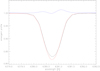 |
Fig. C.1 N IV 6380 for a hot dwarf model (d2v). Black: line profile resulting from our current approach, when manipulating the source functions of EUV background lines with no information on the upper level, as described in the text. Blue: line profile when the EUV two-level-atom source functions are not manipulated. Red: line profile as calculated from our previous FASTWIND version, v10. |
To cure this problem, our code checks for potential overlaps between exact lines and lines with unknown upper level. If the exact line is stronger, we reset the source function of the approximate one, to the value from the exact line. Otherwise, nothing needs to be done. We have tested this approach by comparing between models including or excluding this procedure. Indeed, in most cases there is no effect at all, and only in few cases such as N IV 6380, we see considerable changes (black profile in Fig. C.1).
References
- Abbott, B. P., Abbott, R., Abbott, T. D., et al. 2016, Phys. Rev. Lett., 116, 061102 [Google Scholar]
- Abbott, B. P., Abbott, R., Abbott, T. D., et al. 2017, Phys. Rev. Lett., 119, 161101 [NASA ADS] [CrossRef] [PubMed] [Google Scholar]
- Abdul-Masih, M., Sana, H., Sundqvist, J., et al. 2019, ApJ, 880, 115 [NASA ADS] [CrossRef] [Google Scholar]
- Abdul-Masih, M., Sana, H., Conroy, K. E., et al. 2020, A&A, 636, A59 [CrossRef] [EDP Sciences] [Google Scholar]
- Allen, C. W. 1973, Astrophysical Quantities, 3rd edn. (London: Athlone Press) [Google Scholar]
- Asplund, M., Grevesse, N., & Sauval, A. J. 2005, ASP Conf. Ser., 336, 25 [Google Scholar]
- Bergemann, M., Lind, K., Collet, R., Magic, Z., & Asplund, M. 2012, MNRAS, 427, 27 [NASA ADS] [CrossRef] [Google Scholar]
- Berghoefer, T. W., Schmitt, J. H. M. M., & Cassinelli, J. P. 1996, A&AS, 118, 481 [NASA ADS] [CrossRef] [EDP Sciences] [Google Scholar]
- Bouret, J.-C., Hillier, D. J., Lanz, T., & Fullerton, A. W. 2012, A&A, 544, A67 [Google Scholar]
- Brandt, J. C., Heap, S. R., Beaver, E. A., et al. 1998, AJ, 116, 941 [NASA ADS] [CrossRef] [Google Scholar]
- Bresolin, F., Crowther, P. A., & Puls, J., eds. 2008, IAU 250 Massive Stars as Cosmic Engines (Cambridge: Cambridge University Press) [Google Scholar]
- Butler, K., & Giddings, J. R. 1985, Newsl. Anal. Astron. Spectra, 9 [Google Scholar]
- Carneiro, L. P., Puls, J., Sundqvist, J. O., & Hoffmann, T. L. 2016, A&A, 590, A88 [NASA ADS] [CrossRef] [EDP Sciences] [Google Scholar]
- Chlebowski, T., & Garmany, C. D. 1991, ApJ, 368, 241 [NASA ADS] [CrossRef] [Google Scholar]
- Cohen, D. H., Leutenegger, M. A., Wollman, E. E., et al. 2010, MNRAS, 405, 2391 [NASA ADS] [Google Scholar]
- Donati, J.-F., Howarth, I. D., Jardine, M. M., et al. 2006, MNRAS, 370, 629 [NASA ADS] [CrossRef] [Google Scholar]
- Evans, C., Hunter, I., Smartt, S., et al. 2008, The Messenger, 131, 25 [NASA ADS] [Google Scholar]
- Evans, C. J., Taylor, W. D., Hénault-Brunet, V., et al. 2011, A&A, 530, A108 [NASA ADS] [CrossRef] [EDP Sciences] [Google Scholar]
- Feldmeier, A. 1995, A&A, 299, 523 [NASA ADS] [Google Scholar]
- Feldmeier, A., Kudritzki, R.-P., Palsa, R., Pauldrach, A. W. A., & Puls, J. 1997, A&A, 320, 899 [NASA ADS] [Google Scholar]
- Fullerton, A. W., Massa, D. L., & Prinja, R. K. 2006, ApJ, 637, 1025 [NASA ADS] [CrossRef] [Google Scholar]
- Gräfener, G., & Hamann, W. R. 2005, A&A, 432, 633 [NASA ADS] [CrossRef] [EDP Sciences] [Google Scholar]
- Gräfener, G., Koesterke, L., & Hamann, W.-R. 2002, A&A, 387, 244 [NASA ADS] [CrossRef] [EDP Sciences] [Google Scholar]
- Grevesse, N., & Sauval, A. J. 1998, Space Sci. Rev., 85, 161 [Google Scholar]
- Grin, N. J., Ramírez-Agudelo, O. H., de Koter, A., et al. 2017, A&A, 600, A82 [NASA ADS] [CrossRef] [EDP Sciences] [Google Scholar]
- Hamann, W.-R. 1980, A&A, 84, 342 [NASA ADS] [Google Scholar]
- Hamann, W.-R. 1981, A&A, 93, 353 [NASA ADS] [Google Scholar]
- Harnden, Jr. F. R., Branduardi, G., Gorenstein, P., et al. 1979, ApJ, 234, L51 [NASA ADS] [CrossRef] [Google Scholar]
- Hauschildt, P. H. 1992, J. Quant. Spectr. Rad. Transf., 47, 433 [Google Scholar]
- Hillier, D. J., & Miller, D. L. 1998, ApJ, 496, 407 [NASA ADS] [CrossRef] [Google Scholar]
- Hillier, D. J., & Miller, D. L. 1999, ApJ, 519, 354 [NASA ADS] [CrossRef] [Google Scholar]
- Hillier, D. J., Kudritzki, R. P., Pauldrach, A. W., et al. 1993, A&A, 276, 117 [NASA ADS] [Google Scholar]
- Hillier, D. J., Lanz, T., Heap, S. R., et al. 2003, ApJ, 588, 1039 [NASA ADS] [CrossRef] [Google Scholar]
- Hubeny, I. 1998, ASP Conf. Ser., 138, 139 [Google Scholar]
- Hubeny, I., & Mihalas, D. 2014, Theory of Stellar Atmospheres (Princeton, NJ: Princeton University Press) [Google Scholar]
- Hubeny, I., Hummer, D. G., & Lanz, T. 1994, A&A, 282, 151 [NASA ADS] [Google Scholar]
- Hummer, D. G., & Mihalas, D. 1967, ApJ, 150, L57 [NASA ADS] [CrossRef] [Google Scholar]
- Hummer, D. G., & Mihalas, D. 1988, ApJ, 331, 794 [NASA ADS] [CrossRef] [Google Scholar]
- Krtička, J., & Kubát, J. 2017, A&A, 606, A31 [NASA ADS] [CrossRef] [EDP Sciences] [Google Scholar]
- Kubát, J., Puls, J., & Pauldrach, A. W. A. 1999, A&A, 341, 587 [NASA ADS] [Google Scholar]
- Lamers, H. J. G. L. M., & Morton, D. C. 1976, ApJS, 32, 715 [NASA ADS] [CrossRef] [Google Scholar]
- Lamers, H. J. G. L. M., Cerruti-Sola, M., & Perinotto, M. 1987, ApJ, 314, 726 [NASA ADS] [CrossRef] [Google Scholar]
- Langer, N., Heger, A., & Fliegner, J. 1997, IAU Symp., 189, 343 [NASA ADS] [Google Scholar]
- Langer, N., Schürmann, C., Stoll, K., et al. 2020, A&A, 638, A39 [CrossRef] [EDP Sciences] [Google Scholar]
- Lenorzer, A., Mokiem, M. R., de Koter, A., & Puls, J. 2004, A&A, 422, 275 [NASA ADS] [CrossRef] [EDP Sciences] [Google Scholar]
- Lucy, L. B. 1971, ApJ, 163, 95 [NASA ADS] [CrossRef] [Google Scholar]
- Lucy, L. B. 1982, ApJ, 255, 278 [NASA ADS] [CrossRef] [Google Scholar]
- Lucy, L. B., & Solomon, P. M. 1970, ApJ, 159, 879 [NASA ADS] [CrossRef] [Google Scholar]
- Maeder, A., & Meynet, G. 2000, ARA&A, 38, 143 [Google Scholar]
- Maeder, A., & Meynet, G. 2015, IAU Symp., 307, 9 [Google Scholar]
- Maeder, A., & Zahn, J.-P. 1998, A&A, 334, 1000 [NASA ADS] [Google Scholar]
- Marchant, P., Langer, N., Podsiadlowski, P., Tauris, T. M., & Moriya, T. J. 2016, A&A, 588, A50 [NASA ADS] [CrossRef] [EDP Sciences] [Google Scholar]
- Marcolino, W. L. F., Bouret, J., Martins, F., et al. 2009, A&A, 498, 837 [NASA ADS] [CrossRef] [EDP Sciences] [Google Scholar]
- Markova, N., Puls, J., & Langer, N. 2018, A&A, 613, A12 [NASA ADS] [CrossRef] [EDP Sciences] [Google Scholar]
- Martins, F., & Hillier, D. J. 2012, A&A, 545, A95 [NASA ADS] [CrossRef] [EDP Sciences] [Google Scholar]
- Martins, F., Escolano, C., Wade, G. A., et al. 2012, A&A, 538, A29 [NASA ADS] [CrossRef] [EDP Sciences] [Google Scholar]
- Mihalas, D. 1978, Stellar Atmospheres, 2nd edn. (San Francisco: W. H. Freeman and Co.) [Google Scholar]
- Mihalas, D., Kunasz, P. B., & Hummer, D. G. 1975, ApJ, 202, 465 [NASA ADS] [CrossRef] [Google Scholar]
- Mokiem, M. R., de Koter, A., Puls, J., et al. 2005, A&A, 441, 711 [NASA ADS] [CrossRef] [EDP Sciences] [Google Scholar]
- Najarro, F. 2006, J. Phys. Conf. Ser., 54, 224 [CrossRef] [Google Scholar]
- Najarro, F., Hillier, D. J., Puls, J., Lanz, T., & Martins, F. 2006, A&A, 456, 659 [NASA ADS] [CrossRef] [EDP Sciences] [Google Scholar]
- Najarro, F., Hanson, M. M., & Puls, J. 2011, A&A, 535, A32 [NASA ADS] [CrossRef] [EDP Sciences] [Google Scholar]
- Ng, K. C. 1974, J. Chem. Phys., 61, 2680 [NASA ADS] [CrossRef] [Google Scholar]
- Nieva, M. F., & Przybilla, N. 2012, A&A, 539, A143 [NASA ADS] [CrossRef] [EDP Sciences] [Google Scholar]
- Olson, G. L., Auer, L. H., & Buchler, J. R. 1986, J. Quant. Spectr. Rad. Transf., 35, 431 [Google Scholar]
- Oskinova, L. M., Hamann, W.-R., & Feldmeier, A. 2007, A&A, 476, 1331 [NASA ADS] [CrossRef] [EDP Sciences] [Google Scholar]
- Owocki, S. P. 1994, Ap&SS, 221, 3 [NASA ADS] [CrossRef] [Google Scholar]
- Owocki, S. P.,& Cohen, D. H. 1999, ApJ, 520, 833 [NASA ADS] [CrossRef] [Google Scholar]
- Owocki, S. P.,& Rybicki, G. B. 1984, ApJ, 284, 337 [NASA ADS] [CrossRef] [Google Scholar]
- Owocki, S. P., Castor, J. I., & Rybicki, G. B. 1988, ApJ, 335, 914 [NASA ADS] [CrossRef] [Google Scholar]
- Owocki, S. P., Sundqvist, J. O., Cohen, D. H., & Gayley, K. G. 2013, MNRAS, 429, 3379 [NASA ADS] [CrossRef] [Google Scholar]
- Pauldrach, A. W. A., Kudritzki, R. P., Puls, J., Butler, K., & Hunsinger, J. 1994, A&A, 283, 525 [Google Scholar]
- Pauldrach, A. W. A., Hoffmann, T. L., & Lennon, M. 2001, A&A, 375, 161 [NASA ADS] [CrossRef] [EDP Sciences] [Google Scholar]
- Petit, V., Massa, D. L., Marcolino, W. L. F., et al. 2011, IAU Symp., 272, 206 [Google Scholar]
- Petit, V., Keszthelyi, Z., MacInnis, R., et al. 2017, MNRAS, 466, 1052 [NASA ADS] [CrossRef] [Google Scholar]
- Puls, J. 1987, A&A, 184, 227 [NASA ADS] [Google Scholar]
- Puls, J. 1991, A&A, 248, 581 [NASA ADS] [Google Scholar]
- Puls, J. 2008, Massive Stars as Cosmic Engines, IAU Symp., 250, eds. F. Bresolin, P. A. Crowther, & J. Puls (Cambridge: Cambridge University Press) [Google Scholar]
- Puls, J. 2017, IAU Symp., 329, 435 [Google Scholar]
- Puls, J. 2020, in Radiative Transfer in Stellar and Planetary Atmospheres, eds. L. Crivellari, S. Símón-Diaz, & M. J. Arévalo, Canary Islands Winter School of Astrophysics (Cambridge: Cambridge University Press), 151 [Google Scholar]
- Puls, J., Owocki, S. P., & Fullerton, A. W. 1993, A&A, 279, 457 [NASA ADS] [Google Scholar]
- Puls, J., Urbaneja, M. A., Venero, R., et al. 2005, A&A, 435, 669 [NASA ADS] [CrossRef] [EDP Sciences] [Google Scholar]
- Puls, J., Markova, N., Scuderi, S., et al. 2006, A&A, 454, 625 [NASA ADS] [CrossRef] [EDP Sciences] [Google Scholar]
- Puls, J., Vink, J. S., & Najarro, F. 2008, A&ARv, 16, 209 [NASA ADS] [CrossRef] [EDP Sciences] [Google Scholar]
- Raymond, J. C., Cox, D. P., & Smith, B. W. 1976, ApJ, 204, 290 [NASA ADS] [CrossRef] [Google Scholar]
- Repolust, T., Puls, J., Hanson, M. M., Kudritzki, R.-P., & Mokiem, M. R. 2005, A&A, 440, 261 [NASA ADS] [CrossRef] [EDP Sciences] [Google Scholar]
- Rivero González, J. G., Puls, J., & Najarro, F. 2011, A&A, 536, A58 [NASA ADS] [CrossRef] [EDP Sciences] [Google Scholar]
- Rivero González, J. G., Puls, J., Najarro, F., & Brott, I. 2012a, A&A, 537, A79 [NASA ADS] [CrossRef] [EDP Sciences] [Google Scholar]
- Rivero González, J. G., Puls, J., Najarro,F., & Massey, P. 2012b, A&A, 543, A95 [NASA ADS] [CrossRef] [EDP Sciences] [Google Scholar]
- Rogerson, J. B., J., & Upson, W. L., I. 1977, ApJS, 35, 37 [NASA ADS] [CrossRef] [Google Scholar]
- Rybicki, G. B., & Hummer, D. G. 1991, A&A, 245, 171 [NASA ADS] [Google Scholar]
- Rybicki, G. B., & Hummer, D. G. 1994, A&A, 290, 553 [NASA ADS] [Google Scholar]
- Sana, H., Rauw, G., Naze, Y., Gosset, E., & Vreux, J.-M. 2006, MNRAS, 372, 661 [NASA ADS] [CrossRef] [Google Scholar]
- Sander, A., Shenar, T., Hainich, R., et al. 2015, A&A, 577, A13 [NASA ADS] [CrossRef] [EDP Sciences] [Google Scholar]
- Sander, A. A. C., Hamann, W. R., Todt, H., Hainich, R., & Shenar, T. 2017, A&A, 603, A86 [NASA ADS] [CrossRef] [EDP Sciences] [Google Scholar]
- Santolaya-Rey, A. E., Puls, J., & Herrero, A. 1997, A&A, 323, 488 [NASA ADS] [Google Scholar]
- Schure, K. M., Kosenko, D., Kaastra, J. S., Keppens, R., & Vink, J. 2009, A&A, 508, 751 [NASA ADS] [CrossRef] [EDP Sciences] [Google Scholar]
- Seward, F. D., Forman, W. R., Giacconi, R., et al. 1979, ApJ, 234, L55 [NASA ADS] [CrossRef] [Google Scholar]
- Simón-Díaz, S., Castro, N., Garcia, M., & Herrero, A. 2011a, IAU Symp., 272, 310 [Google Scholar]
- Simón-Díaz, S., Castro, N., Herrero, A., et al. 2011b, J. Phys. Conf. Ser., 328, 012021 [NASA ADS] [CrossRef] [Google Scholar]
- Simón-Díaz, S., Caballero, J. A., Lorenzo, J., et al. 2015, ApJ, 799, 169 [NASA ADS] [CrossRef] [Google Scholar]
- Snow, T. P. J., & Jenkins, E. B. 1977, ApJS, 33, 269 [NASA ADS] [CrossRef] [Google Scholar]
- Snow, T., & Morton, D. 1976, ApJS, 32, 429 [NASA ADS] [CrossRef] [Google Scholar]
- Sundqvist, J. O., & Puls, J. 2018, A&A, 619, A59 [NASA ADS] [CrossRef] [EDP Sciences] [Google Scholar]
- Sundqvist, J. O., Puls, J., Feldmeier, A., & Owocki, S. P. 2011a, Bull. Soc. R.Sci. Liege, 80, 48 [Google Scholar]
- Sundqvist, J. O., Puls, J., Feldmeier, A., & Owocki, S. P. 2011b, A&A, 528, A64 [NASA ADS] [CrossRef] [EDP Sciences] [Google Scholar]
- Sundqvist, J. O., Puls, J., & Owocki, S. P. 2014, A&A, 568, A59 [NASA ADS] [CrossRef] [EDP Sciences] [Google Scholar]
- Sundqvist, J. O., Björklund, R., Puls, J., & Najarro, F. 2019, A&A, 632, A126 [NASA ADS] [CrossRef] [EDP Sciences] [Google Scholar]
- van Regemorter, H. 1962, ApJ, 136, 906 [NASA ADS] [CrossRef] [Google Scholar]
- Zsargó, J., Hillier, D. J., Bouret, J.-C., et al. 2008, ApJ, 685, L149 [NASA ADS] [CrossRef] [Google Scholar]
This is also true for low-mass stars.
Because of the much larger impact of collisional than radiative processes.
With Zn the heaviest element considered, and Li, Be, B, and Sc discarded because of very low abundances.
As long as the Doppler width of the line-profile is dominated by vmic, which is true in hot stars when aiming at a reasonable resolution of lines also from the heaviest elements.
Adopted in the NLTE CMF transport as a pure Doppler profile. As long as the final formal integral correctly accounts for the actual broadening (for example, Stark- and pressure broadening), this has a marginal effect on the resulting occupation numbers and line-profiles (Hamann 1981; Lamers et al. 1987).
Because of the high line density, this approach would not lead to any advantages in computational time.
Because of the somewhat simpler atomic model for N when used as a background element, and because of the corresponding, less rigorous convergence criterion, see Sect. 2.2.
Though not identical, to allow for a reasonable integration-error control.
For this specific comparison, we used only H and He as explicit elements, such that nitrogen is treated within the selected background, and could be included into the mean.
A small difference to the unit-value results from pressure effects.
Though, compared to CMFGEN, to a lesser degree.
We note that to obtain a fair representation of N IV 6380 in our current standard approach (accounting for line overlaps), we use a specific treatment for some of the background lines that are considered in a more approximate way, see Appendix C.2.
Synthesized from a FASTWIND formal solution.
The lower continuum in the observations at roughly 1220 Å is due to the red Lyα wing, being dominated by interstellar hydrogen.
Here and in the following, we mostly follow the notation by Ow13, but use fX instead of fV, to discriminate the volume filling factor of X-ray emitting material from the volume filling factor associated with “cold,” overdense material (= clumps).
Under the conditions considered by Ow13, radiative and adiabatic cooling rates are equal if ls = rs, whereas, following Feldmeier et al. (1997, Eq. (9)), tc∕tf ≈ 5(v(r)∕uj(r)) ⋅ (ls∕rs), with radiative cooling time tc, dynamical wind flow time tf = r∕v(r), and jump velocity, uj(r).
We note that these numbers, particularly the nitrogen abundance, are different from the values provided in the analysis by Bouret et al. (2012).
We stress that no fit has been aimed at in any of the displayed panels.
With stellar, wind, and X-ray parameters very similar to ours, and assuming spatially constant X-ray volume filling factors.
As a reminder, the frequency displacements considered here, xred … x, are negative, with xred ≥ x, whereas Δx ≥ 0.
We note that in this (and other) cases care has to be taken, since x refers to the frequency displacement with respect to a specific line, here to the blue and red component, respectively.
Such a set-up, in connection with the previous FASTWIND version, has been employed, for example, by Rivero González et al. (2012a), Grin et al. (2017), and Markova et al. (2018), for a quantitative nitrogen spectroscopy of massive stars in the LMC and the Galaxy.
The latter file is also used to provide the line-broadening parameters required for the formal integral.
All Tables
Schematic comparison of FASTWIND v10 and v11 (in red): specific methods and data regarding the treatment of explicit and background elements.
Stellar and wind parameters of our model grid used to check specific details of our new FASTWIND version (v11), and to compare with results from CMFGEN and FASTWIND v10.
Stellar, wind, and X-ray emission parameters common to all our ζ Pup-like models.
All Figures
|
Fig. 1 Effects of level dissolution in the UV (left) and the optical and NIR (right), for models s8a and d6v (see Table 2). Displayed is the deviation of the emergent fluxes,
|
| In the text | |
|
Fig. 2 Mean (relative) differences between the main ionization fractions as predicted by our approximate NLTE description following Puls et al. (2005), and our current “exact solution” (complete NLTE, detailed CMF transport), as a function of τRoss ≤ 1 and v (in km s −1). Displayed are the models with the largest differences (s6a) and the smallest ones (d6v) within our grid. The mean (see Eqs. (6) and (7)) refers to 11 selected elements from C to Ni, and its 1-σ deviation is displayed in gray. The vertical lines indicate the location of the sonic point. |
| In the text | |
|
Fig. 3
|
| In the text | |
|
Fig. 4 Comparison of strategic H and He lines in the optical, for all models from our grid. Black: FASTWIND v11, green: CMFGEN, red: FASTWIND v10, with no blends from other elements. The marker in the lower right indicates a wavelength range of 20 Å, and a vertical extent of 0.5 of the continuum. To enable a better comparison, the spectra have been convolved with a rotational broadening of v sin i = 80 km s−1, and degraded to a resolving power of 10 000. |
| In the text | |
|
Fig. 5 As Fig. 4, but for strategic N III lines. Here, the marker indicates a wavelength range of 2 Å, and 0.2 of the continuum. The positions of the individual components of N III λλ4634−4640−4642 of the cooler objects can be clearly seen in the red FASTWIND v10 profiles. Since most lines are weak, no rotational broadening has been applied. |
| In the text | |
|
Fig. 6 On the formation of the N III λλ4634−4640−4642 emission lines in hot massive stars (here: model s6a, see Table 2). Left: optical emission lines (no broadening, no degrading) for various configurations of the EUV N III resonance lines (around 374 Å) coupled to the upper level (3d) of the optical transitions. See legend, and text. “[X]” means ɛX. Right: corresponding EUV radiation field, Jν(τRoss = 0.24). The insert displays the decisive region, and participating lines. Red: N III resonance lines (three components); green: overlapping O III resonance line (out of a multiplet of 6 components); blue: Fe V line at 374.245 Å. We note that 0.01 Å correspond to 8 km s −1. |
| In the text | |
|
Fig. 7 As Fig. 6, left, but for different micro-turbulent velocities in the NLTE model calculations. To allow for a meaningful comparison of the impact on the occupations numbers alone, the micro-turbulent velocities in the formal integrals have been fixed at 15 km s −1 for all cases. |
| In the text | |
|
Fig. 8 As Fig. 6, left, but for different oxygen abundances (see legend), and “normal” Fe content. We stress the non-monotonic behavior. For increasing ɛO, the emission strength at first increases (until ɛO = 8.1), and then decreases, until strong absorption is produced (for ɛO = 9.5). |
| In the text | |
|
Fig. 9 As Fig. 5 (same scale), but for strategic N IV and N V lines of our hotter models. The blue profiles correspond to models, where specific EUV transitions feeding the lower and upper levels of N IV 6380 and of N V λλ4603-4619 have been treated as isolated lines, i.e., ignoring blends. See text. |
| In the text | |
|
Fig. 10 Distribution of Fe IV,V,VI lines with gf ≥ 0.1 according toour line list, in the range between 900 and 2000 Å. See legend and text. |
| In the text | |
|
Fig. 11 Sythetic UV spectra from FASTWIND (black) and CMFGEN (green), for hot, intermediate, and cool O- and early B-star models. To allow for an easy comparion, all spectra have been convolved with v sin i = 200 km s−1. For model d10v, the range enclosed by red lines is detailed in Fig. 12. |
| In the text | |
|
Fig. 12 Close-up of the region between 1210 or 1220 and 1230 Å, for model d10v. In addition to the “standard” spectra from FASTWIND and CMFGEN (with vmic = 15 km s−1, as in Fig. 11), we display results from a FASTWIND formal solution with vmic = 5 km s −1, and two further sets where specific lines have been discarded from the formal solution in CMFGEN, namely either all Fe IV lines, or all transitions (i.e., from all elements) between energy levels that are predicted, but not observationally identified. For color coding, see legend. All spectra have been calculated with an intrinsic resolution of 0.01 Å or better. In the upper panel, they have been convolved with v sin i = 200 km s−1, as in Fig. 11, whereas in the lower ones no broadening has been applied. |
| In the text | |
|
Fig. 13 X-ray volume filling factor, fX, as a function of log r∕R*, for different shock distributions parameterized according to Eqs. (8) and (12) (see legend, and Table 4), and stellar and wind parameters for our ζ Pup-like model (Table 3). The vertical dotted line denotes the region where cooling and wind flow times are equal, tc = tf. Due to the large mass-loss rate, the ratio ls∕rs remains smaller than unity throughout the wind. |
| In the text | |
|
Fig. 14 X-ray luminosity (in the range 0.1–2.5 keV, and in units of Lbol) as a functionof Ṁ∕v∞, for stellar models with photospheric and wind parameters as in Table 3, but mass-loss rates ranging in between 10−9 and 10−4.5 M⊙ yr−1, and different assumptions on fX(r) (see legend, and Table 4). The dotted lines display linear relations (with respect to the log–log scaling), with slopes m = 1 and 2, to guide the eye. Models to the left of and at the vertical dashed line are optically thin in the X-ray emitting region at all contributing frequencies, i.e., R1 < Rmin for energies between 0.1 and 2.5 keV. See text. |
| In the text | |
|
Fig. 15 Ionization fractions of nitrogen and oxygen, as a function of v(r)∕v∞, for the samestellar model and shock distributions as in Fig. 13. For line-coding, see legends. |
| In the text | |
|
Fig. 16 Synthetic line profiles for the UV resonance doublet of O VI, for the same stellar model and different shock distributions as in Fig. 13 (M1, upper left), and for three other models (M2 to M4) differing in mass-loss rate and clumping properties (see Table. 5). Same color coding as in Fig. 15. Profiles from the smooth-wind models M1 and M2 are close to being identical, though mass-loss rates differ by a factorof four. All spectra have been calculated with a depth dependent “micro-turbulence” (proportional to v(r), with a minimum of 15 km s−1, and a maximum of 0.1v∞), and convolved with v sin i = 220 km s−1. For comparison, the observed COPERNICUS spectrum (at a resolution of 0.2 Å, Snow & Jenkins 1977) is displayed in dark green. The dotted lines at the top display the rest-frame frequencies of the doublet components. The absorption feature around 1215 Å, visible in all synthetic spectra without significant O VI contribution, is stellar Lyβ. Model M1 and M4 and corresponding spectra (for fX = const.) are very similar to those displayed (and discussed) by Zsargó et al. (2008) in their Fig. 1. |
| In the text | |
|
Fig. A.1 CMF mean intensity at Rmax (≈ 120 R*), for a hot dwarf model with Teff = 55 000 kK and a large mass-loss rate, calculated with different approximations for the incident intensity, I−, and different wavelength regimes. All intensities have been taken from the same iteration step, namely the first step after the detailed CMF-treatment has been initiated. Color-coding – black: complete incident intensity including frequency derivative, as described in the text; red: I− = 0; dark blue (mostly blended by turquoise): I− specified only for lines and continua of significant optical depth, gradient neglected; turquoise: I− specified for all frequencies, but gradient neglected; green: approximate pseudo-continuum, as used in the previous FASTWIND version, and still at highest and lowest wavelengths. Left panel: EUV range between 200 and 300 Å; right panel: frequency range around the C IV resonance doublet in the UV. |
| In the text | |
|
Fig. A.2 As Fig. A.1, but for λ = 1500−11 000 Å. The impact of the frequency derivative (turquoise versus black) is clearly visible. Without inclusion, no smooth transition between detailed and approximate treatment (at λmax = 10 000 Å) would be possible. Setting I− to zero at all frequencies (red curve in Fig. A.1) results in a flux-distribution identical to the black one in the optical range, whereas specifying I− ≠ 0 only for optically thick lines and continua, and neglecting the frequency gradient (dark blue curve in Fig. A.1), results in fluxes similar to the turquoise ones. |
| In the text | |
|
Fig. B.1 Prototypical convergence behavior for three different kinds of model calculations (see legend and text). Displayed is the maximum relative change of temperature (regarding all grid-points, dashed) within two consecutive iteration steps, and the corresponding mean of the maximum change within all specified occupation numbers, where the averaging has been performed over all depth-points with τRoss ≤ 1. Left panels: mean maximum change within occupation numbers from explicit elements (HHeN in black and red, HHe in blue); right panels: mean maximum change within occupation numbers from selected background elements. Upper and lower panels: convergence behavior for our hottest dwarf (d2v, see Table 2) and supergiant (s2a) model, respectively. Our convergence criterion for the temperature is displayed by a horizontal dotted line. The vertical lines display the onset of the detailed CMF calculations within λmin and λmax (dotted), the update of the photospheric structure (dashed), and the onset of the Ng-extrapolation scheme for the C, N, O resonancelines (dashed-dotted). See text. |
| In the text | |
|
Fig. C.1 N IV 6380 for a hot dwarf model (d2v). Black: line profile resulting from our current approach, when manipulating the source functions of EUV background lines with no information on the upper level, as described in the text. Blue: line profile when the EUV two-level-atom source functions are not manipulated. Red: line profile as calculated from our previous FASTWIND version, v10. |
| In the text | |
Current usage metrics show cumulative count of Article Views (full-text article views including HTML views, PDF and ePub downloads, according to the available data) and Abstracts Views on Vision4Press platform.
Data correspond to usage on the plateform after 2015. The current usage metrics is available 48-96 hours after online publication and is updated daily on week days.
Initial download of the metrics may take a while.