| Issue |
A&A
Volume 642, October 2020
|
|
|---|---|---|
| Article Number | A87 | |
| Number of page(s) | 21 | |
| Section | Interstellar and circumstellar matter | |
| DOI | https://doi.org/10.1051/0004-6361/202038232 | |
| Published online | 08 October 2020 | |
Unifying low- and high-mass star formation through density-amplified hubs of filaments
The highest mass stars (>100 M⊙) form only in hubs★
1
Instituto de Astrofísica e Ciências do Espaço, Universidade do Porto,
CAUP, Rua das Estrelas,
4150-762
Porto, Portugal
e-mail: This email address is being protected from spambots. You need JavaScript enabled to view it.
2
Department of Physics, Nagoya University,
Furo-cho, Chikusa-ku, Nagoya,
Aichi
464-8602, Japan
Received:
22
April
2020
Accepted:
3
August
2020
Abstract
Context. Star formation takes place in giant molecular clouds, resulting in mass-segregated young stellar clusters composed of Sun-like stars, brown dwarfs, and massive O-type(50–100 M⊙) stars.
Aims. We aim to identify candidate hub-filament systems (HFSs) in the Milky Way and examine their role in the formation of the highest mass stars and star clusters.
Methods. The Herschel survey HiGAL has catalogued about 105 clumps. Of these, approximately 35 000 targets are detected at the 3σ level in a minimum of four bands. Using the DisPerSE algorithm we detect filamentary skeletons on 10′ × 10′ cut-outs of the SPIRE 250 μm images (18′′ beam width) of the targets. Any filament with a total length of at least 55′′ (3 × 18′′) and at least 18′′ inside the clump was considered to form a junction at the clump. A hub is defined as a junction of three or more filaments. Column density maps were masked by the filament skeletons and averaged for HFS and non-HFS samples to compute the radial profile along the filaments into the clumps.
Results. Approximately 3700 (11%) are candidate HFSs, of which about 2150 (60%) are pre-stellar and 1400 (40%) are proto-stellar. The filaments constituting the HFSs have a mean length of ~10–20 pc, a mass of ~5 × 10⁴ M⊙, and line masses (M∕L) of ~2 × 10³ M⊙ pc−1. All clumps with L > 104 L⊙ and L > 105 L⊙ at distances within 2 and 5 kpc respectively are located in the hubs of HFSs. The column densities of hubs are found to be enhanced by a factor of approximately two (pre-stellar sources) up to about ten (proto-stellar sources).
Conclusions. All high-mass stars preferentially form in the density-enhanced hubs of HFSs. This amplification can drive the observed longitudinal flows along filaments providing further mass accretion. Radiation pressure and feedback can escape into the inter-filamentary voids. We propose a “filaments to clusters” unified paradigm for star formation, with the following salient features: (a) low-intermediate-mass stars form slowly (106 yr) in the filaments and massive stars form quickly (105 yr) in the hub, (b) the initial mass function is the sum of stars continuously created in the HFS with all massive stars formed in the hub, (c) feedback dissipation and mass segregation arise naturally due to HFS properties, and explain the (d) age spreads within bound clusters and the formation of isolated OB associations.
Key words: stars: formation / ISM: general / open clusters and associations: general / stars: massive / HII regions
Full Table 1 is only available at the CDS via anonymous ftp to cdsarc.u-strasbg.fr (130.79.128.5) or via http://cdsarc.u-strasbg.fr/viz-bin/cat/J/A+A/642/A87
© ESO 2020
1 Introduction
Star formation in giant molecular clouds produces mass-segregated clusters, with the most massive stars located at the centre (Lada & Lada 2003; Portegies Zwart et al. 2010). The mass function of the resulting stars is similar to the Salpeter mass function. Once formed, massive stars are thought to drive significant feedback and produce ionised (HII) regions (Deharveng et al. 2010; Samal et al. 2018) eventually clearing the natal molecular cloud in ~3–5 Myr (Lada & Lada 2003). Typical formation timescales for high- and low-mass stars are ~105 yr (Behrend & Maeder 2001) and 106 yr respectively;if massive stars form first, the feedback can inhibit the formation of the low-mass stars or even halt it by blowing away the natal cloud. If low-mass stars form prior to high-mass stars (Kumar et al. 2006), this effect can be negated and some properties of nearby star forming regions such as the Orion or the Carina nebulae can be explained.
Not all star formation results in dense clusters with OB stars, and not all clusters remain bound following gas dispersal (Lada & Lada 2003; Portegies Zwart et al. 2010; Krumholz et al. 2019). Star formation in nearby regions such as Taurus, Perseus, Chameleon, and Ophiucus lack the O-stars that can be seen in regions such as Orion, Rosette, M8, W40, and Carina. An intriguing observational property of dense clusters such as the Orion Nebula Cluster (ONC) is the finding by Palla et al. (2007) that old stars are found in the midst of young clusters. The ONC is generally considered to have an age of ~1 Myr (Lada & Lada 2003). However, evidence of an extended star formation history (1.5–3.5 Myr) displaying some dependence on the spatial distribution of stars has also been found (Reggiani et al. 2011).
While lower mass star formation that may lead to dispersed populations in the Milky-Way is reasonably well understood (McKee & Ostriker 2007; Kennicutt & Evans 2012), the challenge so far is in arriving at a universal scenario of star formation that can reconcile the observational properties of a well-studied cluster such as the Carina Nebula (Smith 2006), explaining (a) the formation of the highest mass stars such as Eta Carinae (~120 M⊙), (b) mass segregation, and (c) the origin of the full spectrum of initial mass function, especially accounting for the difference in formation times between high- and low-mass stars, and the feedback effects.
The most massive stars catalogued in the Milky Way are typically 100–150 M⊙, though some authors have claimed the existence of 200–300 M⊙ stars in the R136 cluster (Crowther et al. 2010). Theoretically, even though radiation pressure was thought to set an upper limit on the formation of the most massive star, it is now argued that such a limit does not exist (Krumholz 2015). The proposition that high-mass stars form as scaled-up versions of low-mass stars stems from certain observational similarities between them, such as outflows (Shepherd & Churchwell 1996). Nevertheless, the scaled-up idea is largely propagated by theoretical models based on turbulent core accretion (McKee & Tan 2003), proposing mechanisms to dispel radiation pressure, and even utilising feedback to suppress fragmentation (Krumholz 2006). There remains a persistent lack of evidence to explain the formation of the average O-stars (30–50 M⊙) with main sequence lifetimes of a few million years, and even more, giving rise to stars of >100 M⊙. Furthermore, how the necessary mass reservoir is assembled and tens of solar masses are accreted (rate Ṁ ~ 10−4−10−2 M⊙ yr−1) on a timescale that is widely believed to be about 105 yr is also largely unclear (Kennicutt & Evans 2012; Behrend & Maeder 2001; Krumholz 2015). A handful of claims of discs in targets representative of ~20 M⊙ stars are the best observational evidence of the proto-stellar stage (Zapata et al. 2019), and observations searching for massive pre-stellar cores have declared them to be the “holy grail” (Motte et al. 2018a). Observationally, there remains no evidence of disc accretion at a rate of ~10−3 M⊙ yr−1, and the topic is an ongoing challenge.
The idea that the interstellar medium (ISM) of the Milky Way is organised in filamentary structures and bubbles (Inutsuka et al. 2015) was proposed decades ago (Heiles 1979; Schneider & Elmegreen 1979). Following the Herschel space mission, this view has matured, and the properties of filamentary structures have been quantified. It is now believed that the cold ISM, held as the birthplace of stars, is mostly found to be organised in filamentary structures (André et al. 2010). More than 80% of the dense gas mass (above a column density representing Av > 7) in the nearby star forming regions is shown to be in the form of filaments (Könyves et al. 2015, 2019; Arzoumanian et al. 2019). The star forming clouds in much of the Milky Way are now viewed to be filamentary in nature (Inutsuka et al. 2015). Dense filamentary structures in the Milky Way disc have been uncovered using Galactic-plane surveys such as ATLASGAL and Hi-GAL (Li et al. 2016; Mattern et al. 2018; Schisano et al. 2020), with a wide range in lengths (a few to 100 pc) and line masses (a few hundreds to thousands of M⊙ pc−1).
In a molecular cloud, these filamentary structures inevitably overlap to form a web, creating junctions of filaments. Myers (2009) identified such junctions for the first time, defining them as hubs, objects of low aspect ratio and high-column density, in contrast to filaments that have high aspect-ratio and lower column densities. This author also showed that the nearest young stellar groups are associated with hubs that radiate multiple filaments and pointed out that such a pattern was also found in infrared-dark clouds. Directed by this observational association of hubs and clusters, many authors have studied hub-filament systems (HFSs) as possible progenitors of proto-clusters and high-mass star formation (Schneider et al. 2012; Mallick et al. 2013). Young stellar clusters (YSCs) can be split up according to mass, with the highest mass stars located at the centre, which prompted other authors to investigate high-mass star formation in HFSs (Liu et al. 2012; Peretto et al. 2013). These studies clearly demonstrate the role of HFSs as important observational targets to understand both the formation of high-mass stars and YSCs. Observations of HFSs have uncovered longitudinal flows (Peretto et al. 2013, 2014; Williams et al. 2018) within filaments with flow rates of ~10−4–10−3 M⊙ yr−1 (Chen et al. 2019; Treviño-Morales et al. 2019). Because such flows are found to converge to a cluster of stars (Chen et al. 2019; Treviño-Morales et al. 2019), it has been argued that the flow, triggered by a hierarchical global collapse, provides sufficient flow rates to form massive stars. Hubs with either a few (Williams et al. 2018; Chen et al. 2019) or a large network of filaments (Treviño-Morales et al. 2019) both report similar flow rates, which leads us to pose the following questions; what is the difference between such HFSs with few filaments and large network of filaments? Are the flows driven by a pre-existing massive star/ clusters gravitational potential drives or if the formation of the massive star is a consequence of the flows? These observations of early to intermediate stages of cluster formation will always be plagued by the uncertainty of whether or not fragmentation-induced starvation limits the formation of the most massive stars (Peters et al. 2010).
Here we approach the problem in reverse order by asking whether or not the highest luminosity (therefore, highest mass) stars that have recently formed are associated with HFSs, and if so, what it is that makes these regions unique. The Herschel Hi-GAL survey has led to an unprecedented and unbiased sample of star-forming clumps in the entire Milky Way disc. The low aspect ratio and high column density of hubs can make them appear similar to any star-formingclump of dense gas. However, not all clumps can be hubs; especially when considering the results from Myers (2009), that hubs coincide with the centres of stellar groups. The fraction of cluster-forming hubs must be quite small when compared to all the clumps in a giant molecular cloud. Additionally, for an observer, line-of-sight coincidences of filamentary structures may mimic a hub-like structure. In the filamentary paradigm of molecular clouds, there are main filaments, sub-filaments, and striations, as well as junctions of each of these structures which can in principle also be called a hub. By this definition, the hubs defined by Myers (2009) represent junctions of main filaments, and there should be a hierarchical distribution of hubs depending on the type- and number of elements intersecting to form a hub. The nature of the star formation that takes places in hubs will then depend upon the nature of these junctions, resulting from the density and number of intersecting filamentary structures.
Therefore, it is unclear whether or not every HFS leads to the formation of high-mass stars and/or clusters and the current study is just the beginning of what we may learn by observing these systems. However, given the unambiguous importance of HFSs, it is necessary to first identify such systems in an unbiased way. This work aims to identify candidate HFSs towards the inner Galactic plane using Hi-GAL data. The analysis is different from other “filament catalogues” of the Galactic plane (e.g. Li et al. 2016; Schisano et al. 2020) because it does not search for filaments but is looking at filaments merging into clumps. Section 2 describes the data sets used to conduct the search. Section 3 details the definitions and methods of identification of filamentary structures and hubs and Sect. 4 reports the results and describes the output products. Based on the results, we present and discuss a “filaments to clusters” paradigm for star formation in Sect. 5. In Sect. 6 we compare this paradigm with the literature and some archival data of two nearby regions of cluster formation namely NGC 2264 and W40. In Sect. 7, we compare the HFS paradigm with other models of cluster formation. In Sect. 8 we discuss the implications of the HFS paradigm for the hierarchy of HFSs and observations of massive discs and pre-stellar cores, and its relevance to the formation of very massive stars, feedback, and triggered star formation.
2 Observational data
We used 250 μm maps, column density maps, and the clumps catalogue from the Herschel Hi-GAL survey to search for filamentary structures and hubs. The Herschel Infra-red Galactic plane survey (Hi-GAL; Molinari et al. 2010, 2016) covered the inner part of the Galactic Plane (68° ≥ l ≥−70° and |b| ≤ 1°) using PACS (Poglitsch et al. 2010) 70 and 160 μm and SPIRE (Griffin et al. 2010) at 250, 350, and 500 μm simultaneous imaging in all five bands. These data were reduced using the ROMAGAL data-processing code, for both PACS and SPIRE (see Traficante et al. 2011 for details). Images of the four bands from 160 to 500 μm were then used to compute the column density and the dust temperature (Td) maps. A catalogue of Hi-GAL clumps was prepared by Elia et al. (2017), which contain ~105 sources. This catalogue lists various properties of the detected clumps such as the full width half maximum, luminosity, distance, surface density, and proto or pre-stellar nature of the clump. Identification of clumps is based on the photometriccatalogue, the details of which can be found in Molinari et al. (2016). The sources are extracted using bi-dimensional Gaussian fits to the source profile using the CuTEx algorithm (Molinari et al. 2011); we strived to achieve completeness in each band. Typically, a 90% completeness limit on the Hi-GAL clump catalogue yields 5 M⊙ clumps at 1 kpc distance.
In this work, the distances provided by the clump catalogue (Elia et al. 2017) have been updated based on the distances provided by Urquhart et al. (2018). For those clumps where distances are not available, if they are enclosed in the star-forming region of a known distance, that distance is assumed.
Targets and data selection
In order to identify HFSs, it is necessary to examine the filamentary structures around every known Hi-GAL clump, and evaluate if it represents an intersection of filamentary structures. Given that HFSs are known to be associated with YSCs, and our interest in studying high-mass star and proto-cluster formation, the requirement here is in the robustness of the target clumps rather than completeness. To obtain a robust sample of clump targets, we conducted a quality analysis and cut to the sources in the original Hi-GAL catalogue. The quality-controlled sample-selection criteria are as follows:
-
Detection at all four bands from 160 to 500 μm (71% of the total sample: 44 686 sources).
-
Peak position precision between two consecutive bands within 3σ of the positional offsets of all sources (of any flux) in a given band (60% of the sources remaining – 37 494).
-
3σ flux detection in all four bands (55% – 34 575).
The total number of target clumps satisfying all the above criteria is therefore 34 575. There are 145 sources that are saturated in one or all bands; we modelled and corrected these, and have included them in the above quality-controlled sample.
Given that the targets are located at a wide range of distances from within the solar neighbourhood all the way up to 10–12 kpc, angular resolution is an important criterion to maximise the output of our filamentary-feature detection. Therefore, we perform our HFS search using the 250 μm images that are considered to be the best representation of column density while having a superior angular resolution (18.2′′ beam FWHM) compared to the column density maps at 36′′ resolution. We extracted 10′ × 10′ images of the calibrated 250 μm maps around each of the 34 575 targets to identify the filamentary structures.
3 Identifying filamentary structures and hubs
3.1 The DisPerSE algorithm
The Discrete Persistent Structures Extractor (DisPerSE) software (Sousbie 2011) was used to identify filamentary skeletons in each of the above image cut-outs. DisPerSE is designed to identify persistent topological features such as filamentary structures, voids, and peaks. It works by connecting critical points such as maxima and minima with integral lines along the gradients in a given map. Critical points correspond to a zero gradient on the map. One of the important inputs for the algorithm to run is “persistence level” which is the absolute difference between the values of the critical points, or in other words, between the maxima and minima along a gradient that is connected by a single integral line called an “arc”.
Persistence Level and Background
The target clumps are spread along the Milky Way plane, so the background varies significantly between clumps. The mean intensity value of the background (mode of the intensity, explained further ahead) on the 250 μm image (10′ × 10′ cut-outs) varies between 10 and ~18 000, with a standard deviation of ~800, all in units of MJy Sr−1. This corresponds to column density variations between 9 × 10¹⁹ and 1.5 × 1023cm−2 on the cut-outs. These numbers demonstrate that in some cases the cut-out image is filled mostly by the emission from the dense clump and in some cases by the emission surrounding the target clump. Additionally, depending on the intensity of the source, the background-to-source ratio plays an important role in detecting significant filamentary features. We experimented in running DisPerSE on 250 μm images and an unsharp masked version where the background was subtracted by a smoothing equal to 1.5 times the beam width. Comparing the results, it was found that DisPerSE can efficiently detect features even in a noisy image without background subtraction, provided a correct background is determined. In Fig. 1 we display the pixel distribution histograms of two images, demonstrating the nature of pixel distribution in the image that is dominated by background emission and another where the dense clump is bright compared to the background. By definition, mode is the peak of the pixel distribution histogram, which represents the “background” or “most common” value, shown by a red line. Another useful quantity is the “midpoint” which is estimated by integrating the histogram and computing by interpolation of the data value at which exactly half the pixels are below that data value and half are above it. In IRAF, both mode and midpoint are computed in two passes, unlike statistics such as the mean, standard deviation, and so on. In the first pass the standard deviation of the pixels is computed and used with the bin-width parameter to compute the resolution of the data histogram. In the second pass, the mode is computed by locating the maxima of the data histogram and fitting the peak by parabolic interpolation. The midpoint is typically larger than the mode, as shown by the red and green lines in Fig. 1.
We define the persistence level for each source as five times the standard deviation of the pixels below the midpoint value. We note that the midpoint is fairly close to the mode or the background, while ensuring that half the pixels in the distribution histogram are considered. This is a conservative choice, made after experimenting by setting the persistence level as the standard deviation of the pixels below the mode and midpoint. All detected skeletons are therefore above the 5σ level of the background variations in each target. Many of the Hi-GAL clumps are located in the midst of giant molecular clouds or HII regions, where the estimated background represents the ambient column density of the cloud or nebulosity. In that casethe chosen persistence level is set to pick up skeletons well above the inter-cloud column density fluctuations.
The DisPerSE algorithm is executed on the 250 μm cut-out image of each target using the respective persistence level. This is accomplished by running the main task mse within the algorithm. In the next step, DisPerSE builds “skeletons” of crests traced by the arcs above the given persistence level. Aligned arcs are assembled into individual skeletons, with the alignment defined by a critical angle between two consecutive arcs. We set this angle at 55°, similar to previous methods of filament detection (e.g. Arzoumanian et al. 2019). Each skeleton assembled is tagged by a number that is based on the order in which it was detected: the skeleton picked up first by the algorithm will be assigned the value 1, and so on. This skeleton tag is a useful indicator of the prominence of the detected features. This step is accomplished by running the task skelconv. The result of the above two steps is a fits file with all identified skeletons above a certain persistence level, tagged with respective numbers.
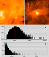 |
Fig. 1 Pixel value distribution histogram examples of 10′ × 10′ cut-out maps of (A) Background-dominated image, and (B) source-clump-dominated image. The x-axes of the histograms denote the pixel intensity values in MJy Sr−1. The red andgreen vertical lines mark the mode and midpoint respectively. |
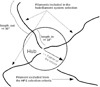 |
Fig. 2 Hub-filament systems selection criteria. |
3.2 Selecting the hub-filament systems
The working definition of a filament is that it should have an aspect ratio of at least three, Lfil ∕Wfil ≥ 3, as defined by previous exercises (Arzoumanian et al. 2019; Könyves et al. 2019). Given that the width of the filament Wfil is unresolved in almost all the cases for the very distant targets in this study, the width is defined by the beam size at 250 μm (18.2′′); therefore, a skeleton should have a length Lfil ≥ 55′′ to be considered as a filament. The definition of a HFS is sketched in Fig. 2. At the outset, a hub is defined as a junction of three or more skeletons at the source centre. The source size varies as the full width at half maximum (FWHM) of the detected clump. Any filament is considered to meet at the source if at least one beam width, represented by three native pixels (6′′ × 3 = 18′′) of the skeleton, falls within the source FWHM. We note that DisPerSE is highly effective in picking up every filamentary structure, not all of which can be considered prominent by a visual inspection, especially when dealing with weak clumps or targets located at large distances. Also, sometimes, the algorithm selects linear structures at the edges of the images that should be clipped away. Therefore, we imposed two additional criteria; (a) that every pixel of the skeleton should have a minimum intensity of 3σ (σ of pixels belowthe midpoint value, see Sect. 3.1) in order to be included in the HFS criteria, and (b) only the first half of detected skeletons (identified by the number tagged by DisPerSE to the skeleton) are considered. The second constraint is effective in clipping away unwanted edge-of-the-image structures and very small skeleton branches of low intensity. All targets that satisfied the above two criteria along with that defined in Fig. 2. were selected as candidate HFSs.
The above criterion was not applied to saturated sources because the intensities in the central regions are modelled by Gaussian fitting and the saturated sources generally fill a large fraction of the 10′ × 10′ cut-outs, strongly influencing the background value by the large-scale nebular emission. Instead, the only constraint imposed was that a filament should have non-zero length within the FWHM of the clump in order to be considered as a hub. The FWHMs of the saturated sources are also larger than those of the non-saturated clumps. Visual examination shows dense networks of filaments in every source (see Fig. 13).
A catalogue was assembled listing the indicative properties of the filaments and the associated clump properties. The total filament lengths were separated into length inside and outside the clump. An indicative column density of the respective parts of the skeleton was computed by reading out the values of each skeleton pixel from the Hi-GAL column density maps. Also, the total column density within a circle of radius equal to the source FWHM was computed. For each target, the mode from the column density maps of 10′ × 10′ (similar to the 250 μm maps) was used as a background value that was subtracted from the column densities read out for each skeleton pixel. A sample of the HFS catalogue is shown in Table 1 and the full list is made available via CDS and Vizier platforms.
The filament mass was computed using the measured column density NH and using the formula MFIL = NH
 × areaFil × μH_2 × mH where μH_2 is the mean molecular weight per H2 taken as 2.33 and mH is the atomic weight of hydrogen. The filament length is multiplied by one pixel width (6′′) to obtain the areaFil. Additionally, we also provide overlays of HFS skeletons on the 250 μm images for visualisation of the candidate systems as shown in Fig. 3a.
Catalogue of hub-filament system candidates.
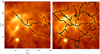 |
Fig. 3 Example of an HFS candidate: skeletons passing the HFS criteria (left panel) and all skeletons selected by DisPerSE (right panel) are overlaid on a 250 μm image. |
3.3 Column density profile of hub-filament systems
The DisPerSE output skeletons were used as a mask on the corresponding column density map cut-outs of each target, allowing us to measure it along the filaments and clumps located on the filaments. The result is shown in the left panel of Fig. 5. These masked column density maps of all HFS and non-HFS targets were averaged to produce the middle and right panel images in Fig. 5. In this averaged image, the central pixel corresponds to the clump centre. Next, we computed the average column density value in concentric circles of one pixel width with respect to this centre, to produce circularly averaged radial profiles shown in Fig. 11. The standard deviation of this circular average is used as the corresponding error in the figure. Such profiles were computed for pre-stellar and proto-stellar sources separately in the HFS and non-HFS groups.
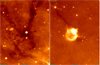 |
Fig. 4 Hub-filament examples as viewed by the Spitzer 8 μm images: candidate HFSs may be composed of filaments that are infrared dark (left) or bright, or a combination of infrared-dark and bright features (right). |
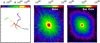 |
Fig. 5 Computing the column density profile for HFSs: the column density map of each target is masked by the skeleton (left panel) and then averaged for all target hubs (middle panel) and non-hubs (right panel). The radial profile shown in Fig. 11 is computed using these average images for different evolutionary groups. The example shown here is for the group of proto-stellar hubs and non-hubs, and the units of the colour bar are cm−2. |
4 Results
In searching the 34 575 Hi-GAL clumps with the methods described above, we found 3704 HFSs. Of these, 144 are saturated sources, all of which are identified as HFSs. This implies that ~10.7% of the Hi-GAL clumps are located at the line-of-sight junction of filamentary structures. Other clumps which are located on a single filament or at the junction of two filaments are called non-hubs in the following. There are 26 135 non-hub clumps, of which 10 380 are located at the junction of two filament skeletons and 15 755 form the tip of a single filament. Many of these latter 10 380 non-hub clumps may simply represent a clump that is actually located somewhere along a single filament. There are also 4736 clumps that are not associated with any filaments (0 skeletons) and are not included in further analyses. Using the evolutionary state classification in the Hi-GAL catalogue, we find that 156 (4%), 2010 (54%), and 1537 (41%) of the 3704 HFSs are respectively classified as starless, pre-stellar, and proto-stellar in nature. All 144 clumps that are saturated in one or moreof the Herschel bands are proto-stellar in nature and they are among the most active sites of star formation.
Inspection of the skeleton overlays on the images reveals that the filamentary structures detected here can represent either (a) cold dense filaments such as infrared-dark clouds that are conducive to star formation, or (b) emission nebulae and similar structures (e.g.: edge of a dusty shell or bubble illuminated by a massive star) with significant dust column density located in an already active star forming region. The distinction between such targets will require multi-wavelength examination. For example, in Fig. 4 we display Spitzer IRAC 8 μm images of two hubs demonstrating that a hub may represent any combination of 8 μm dark and bright filamentary structures.
We find that the identified HFSs are composed of up to seven filaments joining at the hub. By examining the images of some of the brightest sources, especially saturated sources, it is evident that there are many more filamentary features visible on the images that have not passed the series of selection criteria used in the detection method described above. This is because a single uniform criterion that is applied here cannot work at full efficiency for the variety of targeted sources, especially with a complex mixture of brightness, background, and structures. Persistence level and selection cuts have to be appropriately fine-tuned to each target in order to extract all features in a given image. Therefore, the upper limit on the number of filamentary structures forming a hub is only moderately represented by the nskel parameter in the HFS catalogue. This analysis however yields a number of prominent skeletons (with S∕N > 5).
4.1 Filament and hub properties
The targets in the studied sample have a range of distances between 100 pc and 24 kpc. The Hi-GAL clumps are generally recovered from major areas of star formation, peaking roughly at 3 kpc (Galactic fourth quadrant, central bar), 5 kpc (molecular ring, Sagittarius, and Norma spiral arm tangents), and at 11 kpc (Galactic warp) (e.g. see Fig. 4 in Elia et al. 2017). In Fig. 6, the distance histograms (normalised by the maximum value of each sample) of all the hubs and non-hub clumps are shown, which indicate that the two are similarly represented at all distances. Inclination angles of the HFSs will also play a major role in their detection, especially at these large distances; however, there is no measurement to distinguish those effects. The 18.2′′ beam resolution of the 250 μm images corresponds to the projected scales of 0.26 and 0.7 pc at distances of 3 and 8 kpc, respectively. The filament widths are clearly unresolved in the HFS sample; indeed the HFS detected filaments are either high-line-mass filaments or elongated clouds, and are not comparable to the filaments described by studies of nearby star forming regions in the Gould belt (Arzoumanian et al. 2019). In Fig. 7, we plot the normalised histogram of filament lengths; this is taken as length (in pc) instead of total filament length to ensure that the fraction of the filament within the target clump FWHM is excluded from consideration. We note that, “individual filaments” in the following figures refers to the constituent filaments of non-hub clumps. Figure 7 shows that the hub systems are dominated by longer filaments (mean length ~18 pc) compared to the non-hub clump (mean length ~8 pc) average. Figure 8 displays the normalised histogram of filament masses, where one can see the immediate effect of longer filaments influencing the mass. The mean mass of the HFS filaments (1.4 × 10⁵ M⊙) is higher than that of the non-hub clumps (~6.3 × 10⁴ M⊙). However, this may not be significant given the broad distribution of the masses. For a given sensitivity of the Hi-GAL maps, one of the most profound effects of the limited angular resolution is that at larger distances, only longer filaments can be detected. This is reflected in Figs. 7 and 8. The relation between filament length and mass can be visualised in Fig. 9; at lower masses and shorter lengths, this plot displays a larger scatter when compared to similar plots from studies of filament catalogues (Li et al. 2016; Schisano et al. 2020). This may be the result of detecting filaments on the 250 μm images which has a higher spatial resolution than the column density maps used in the other studies. The striking feature of Figs. 7–9 is that even though the candidate HFSs are uniformly distributed over the distance range traced by the full target sample, HFSs appear to be composed of longer and more massive filaments. It can also be viewed as lower detection of weaker or less massive clumps at large distances. Figure 10 shows the normalised histogram of the filament line mass, indicating a similar distribution for filaments constituting both hub and non-hub systems.
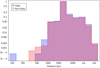 |
Fig. 6 Histograms (normalised by maximum y-value) of distances of all clumps compared with those of HFSs, demonstrating that HFSs are uniformly distributed over the range covered by all clumps. |
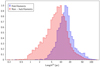 |
Fig. 7 Histogram (normalised by maximum y-value) of filament lengths for HFS and non-HFS samples, showing that HFSs are composed of longer filaments. |
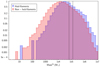 |
Fig. 8 Histogram (normalised by maximum y-value) of filament masses in HFS and non-HFS samples, showing the effect of massive filaments in HFSs. The vertical lines represent the mean values. |
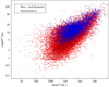 |
Fig. 9 Mass–length relation of the filaments around clumps. |
4.2 Density enhancement and massive star formation in hubs
Circularly averaged radial profiles of column density centred on the clumps located in hubs and non-hubs are shown in Fig. 11. These profiles are also separated for pre-stellar and proto-stellar objects. Targets with saturated pixels are all proto-stellar but they are shown separately to distinguish modelled fluxes using Gaussian fitting from the rest. Moving along the filaments to the clump centre, the column densities of the clumps representing hubs display enhancements when compared to those located in non-hub systems; i.e. clumps located on individual filaments. The ratio of the peak column density at the centre of the clump between the hub and non-hub systems is taken as the enhancement factor which is 1.9 for pre-stellar clumps, 2.1 for proto-stellar sources, and ~10 in saturated sources. It should be noted that most nearby regions of intense star formation, producing the high-luminosity sources, are all saturated in one or more bands.
The distribution of hub and non-hub systems on a luminosity vs. distance plot is shown in Fig. 12. Saturated sources are plotted separately and are all proto-stellar in nature. The two horizontal lines mark the luminosity cuts at 104 L⊙ and 105 L⊙. All clumpswith L > 105 L⊙ located at a distance of ≤5 kpc are hubs, as are the clumps with L > 104 L⊙ at ≤2 kpc. At farther distances, identifying the HFSs by resolving individual filaments is limited by the 18′′ resolution of the 250 μm images. Stars of masses greater than 8 M⊙ are considered massive; however, only in stars with a luminosity L > 104 L⊙ do the radiation and gravitational pressures become roughly equal. Given that essentially all luminous targets at nearby distances are hubs, this means that all massive stars form in hubs, especially those where radiation pressure is considered significant, defined by the Eddington ratio of one.
The results shown in Figs. 11 and 12 lead us to the following corollary; the most natural conditions to form the massive stars arise only when multiple filaments join to form a hub, because this is when the characteristic densities (and mass) of the individual filaments can be instantaneously summed, creating the highest density and most massive pockets of gas and dust. The coalescence scenario by Bonnell et al. (1998) proposed that low-mass stars merge and/or coalesce to form high-mass stars in a high-density environment. In its essence, the corollary above is the coalescence scenario, except that the merging is not of the stars, but of the gas and dust in the fertile (Hacar et al. 2018) filaments.
For majority of the clumps studied (unsaturated in the Herschel bands), the number of skeletons joining at the hub is in the range of 3–7. On the contrary, the saturated sources display large networks of filaments around them, typically 6–12 main filaments. A comparison of the skeleton numbers between saturated and unsaturated clumps is not appropriate because we do not clip the filaments in saturated sources using column density cuts (see Sect. 3.2). Also, filament detection must be improved using 160 and 70 μm data along with that of 250 μm in order to enhance spatial resolution. However, it should be mentioned that in the saturated sources, which represent the most luminous and nearby regions and are bright sources, the column density is high throughout the field. In Fig. 13, we show samples of saturated sources along with the skeletons. These mostly represent major nodes of clustered star formation in giant molecular clouds, such as the ONC. The result shown in Fig. 11 is evidence that HFSs with the largest density increase at the hub (saturated sources) are the result of larger networks of criss-crossing filaments.
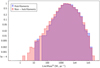 |
Fig. 10 Histograms (normalised by maximum y-value) of filament line mass. |
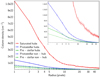 |
Fig. 11 Circularly averaged radial column density profiles centred on the studied clumps. The column density is plotted as a function of pixel (each pixel is an azimuthal average) distance from the centre. The error bars display the standard deviation onthe azimuthal average at each pixel. Saturated proto-stellar clumps are plotted separately because the fluxes are modelled and recovered from Gaussian fitting. |
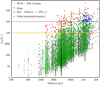 |
Fig. 12 All massive stars form in hubs: all sources with a luminosity L ≥ 105 L⊙ in the inner Milky Way and located at a distance of <5 kpc are found to be HFSs. All hubs are marked by green circles. Clumps (with L ≥ 105 L⊙) that arenot found to be hubs (blue triangles) are located farther than 5 kpc because the 18′′ beam resolution of the data is insufficient to resolve these structures. The yellow line at L = 104 L⊙ indicates the Eddington ratio at which radiation and gravitational pressures become roughly equal; at <2 kpc, all objects above this luminosity are hubs, demonstrating that massive stars preferentially form in hubs. |
5 Filaments to clusters: a paradigm for star formation
These new findings from Sect. 4.2 lead us to build a scenario of star formation in the HFS paradigm as presented in Fig. 14. This scenario is represented by four stages that can be roughly compared with evolutionary snapshots of star formation in molecular clouds. Stages I, II, III, and IV respectively represent low-mass-star formation in filaments without hubs, pre-stellar HFSs surrounded by young clusters of low-mass stars, HFSs with high-mass protostars surrounded by young cluster of low-mass stars, and a full-blown HII region with embedded clusters such as the Orion Nebular Cluster (ONC).
Low- to intermediate-mass star formation alone can take place in individual filaments, whereas high-mass stars form preferentially in hubs. In the following, we elaborate on this scenario using the simplest case of two filaments coming together at a junction and thus forming a hub.
5.1 Stage I: initial conditions
Flow-driven filaments, either due to intra-molecular cloud velocity dispersions (~1 km s−1) or externally driven by expanding shells (~10 km s−1) join to form a hub. Observations of colliding filaments in the Mon OB1 star-forming region show a pair of filaments approaching each other with relative velocities of 2–4 km s−1 (Montillaud et al. 2019). A variety of external triggers can also drive such motions, of which stellar wind bubbles and HII region shells are observationally prominent (see Myers 2009, for a discussion); but late phases of supernova remnants are also important. Such filaments should be similar to the filaments in Taurus (Palmeirim et al. 2013) and are often fertile (Hacar et al. 2018), with ongoing low-mass star formation. This is because large populations of young low-mass stars have been found around high-mass protostars (Kumar et al. 2006) and around HFSs (Dewangan et al. 2017; Baug et al. 2018).
The filaments that set up the initial conditions for the formation of the hub need not necessarily form by gravity and turbulence. Instead, they can form via mechanisms such as cloud–cloud collision where the most basic effect of compression will lead to filament formation. Numerical simulations by Inoue & Fukui (2013) describe the formation of such filaments and also show that they are magnetised (see also Inoue et al. 2018), which is an important aspect in the formation of massive stars as is seen at Stage III. Numerous observational studies (e.g. Fukui et al. 2014; Torii et al. 2015; Sano et al. 2018) are in support of this mechanism. Indeed this may be the prominent mechanism through which hubs with large networks of filaments can form in the most massive clouds, leading to cluster formation. In summary, dense fertile filaments moving towards each other set up the initial conditions of the HFS paradigm.
5.2 Stage II: hub formation – spin and geometry
The filaments can overlap with any relative orientation (0–90°), in such a way that a pre-existing dense core, intra-filamentary material, or a combination of both can form the junction. At small inclination angles, multiple filaments are compressed essentially along the longitudinal axis; this may be the mechanism responsible for the formation of high line-mass (Kainulainen et al. 2017), and a large network of connected filaments (Hacar et al. 2018) such as the Orion integral shaped filament. This would not constitute a hub, even though high-line-mass filaments may form on an average higher-mass cores than their lower mass counterparts (Shimajiri et al. 2019; Könyves et al. 2019). A hub is a relatively low-aspect-ratio object (Myers 2009) and together with its density amplification property (Sect. 4.2) it will always provide enhanced star formation conditions with respect to what is possible within a filament of certain line mass. In other words, a hub can form a massive star that is more massive than the most massive star that can form in the hub-composing filaments. The larger number of filaments in saturated sources together with the density amplification result prompts us to predict that the mass of the most massive star formed will be correlated with the network factor fnet =  where
where  represents the number of filaments with a certain line mass
  .
.
The probability to overlap at a location that is not exactly the centre of mass is high. Therefore, we propose that the approaching filaments can impart a small twist to the hub, giving rise to an initial angular momentum. If the colliding filaments have large line-mass inhomogeneity prior to the collision, the twist and therefore the rotation of the hub is also larger. We suggest that the resulting spin can eventually flatten the hub, a conjecture that can be observationally examined. This may also explain the new ALMA observations of MonR2 (Treviño-Morales et al. 2019) where a spectacular network of filaments can be seen spiralling into the hub. Myers (2009) compared the observed HFSs in nearby regions of star formation to several analytical models and argued that the outer layers are best represented by a modulated Schmid-Burgk equilibrium. He focussed on explaining the formation of hubs and parallel spaced filaments in nearby regions and arrived at a pancake or sheet-like geometry for hubs. Numerical simulations of cloud collision and compression (Vázquez-Semadeni et al. 2007) produce a central shell with outwardly radiating filaments. By any or all of these arguments, a hub is very likely to possess a flattened geometry.
Indeed, a hub is likely to assume an ellipsoidal geometry, and more specifically an oblate spheroid. The mean aspect ratio of hubs from our candidate sample, measured using the 250 μm images, is 1.2 ± 0.4, however ~20% of them have an ellipticity of ~1.5–3.0. The 18′′ angular resolution of the data is insufficient to resolve the ellipticity for all targets, especially when considering projection and distance effects, but it is evident in the high-resolution data of individual targets (Williams et al. 2018; Chen et al. 2019, see also Fig. 4).
A hub with an oblate spheroidal geometry is pre-stellar at this stage, and observationally represented by a massive pre-stellar clump surrounded by a population of low-mass young stellar objects (YSOs). An excellent example representing this stage is the M17SWex, where the infrared dark cloud (IRDC) display approximately 500 YSOs (all low mass, conspicuously lacking massive objects) in the dark cloud (Povich & Whitney 2010) containing at least two hubs (Chen et al. 2019).
In the simplest case of two, typically fertile filaments, the overlap can happen in such a way that a pre-existing dense core, intra-filamentary material, or a combination of both can form the hub. Therefore, a hub will inherit the combined density inhomogeneities of the composing filaments, as depicted in Fig. 14 by the relatively dense left edge of the hub compared to the right at this stage.
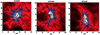 |
Fig. 13 Examples of saturated sources with a large network of filaments. Skeletons are overlaid on 250 μm images. |
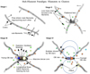 |
Fig. 14 Filaments-to-clusters paradigm for star formation. Flow-driven filaments overlap to form a junction that is called a hub. The hub gains a twist as the overlap point is different from the centre of mass, and the density is enhanced due to the addition of filament densities. Low-mass stars can be ongoing before and during hub formation. The hub gravitational potential triggers and drives longitudinal flows bringing additional matter and further enhancing the density. Hub fragmentation results in a small cluster of stars; however, a pancake or sheet morphology often leads to near-equal mass fragmentation, especially under the influence of magnetic fields and radiative heating. Radiation pressure and ionisation feedback escapes through the inter-filamentary cavities by punching holes in the flattened hub. Finally, the expanding radiation bubbles can create bipolar shaped HII regions, burning out the composing filaments to produce tips that may be similar to the structures called pillars. The net result is a mass-segregated embedded cluster, with a mass function that is the sum of stars continuously created in the filaments and the massive stars formed in the hub. |
5.3 Stage III: massive star formation in the density amplified hub
A hub formed by the junction of filaments is an object experiencing shock. Whitworth et al. (1994) argue that a suddenly compressed layer will switch to become confined by self-gravity, moving from a flat density profile to a centrally condensed density over a time tswitch. This time isof the order of one free-fall time of the uncompressed medium. If we consider the dense gas in the individual filaments as the uncompressed medium, a hub should become gravitationally unstable in ~1–2 Myr after its formation. This time is also similar to the estimated mass doubling time of 1–2 Myr in filaments (Palmeirim et al. 2013). However, a magnetically threaded hub can take longer to begin to collapse.
Having inherited density inhomogeneities at Stage II, the densest portion of the hub begins to collapse first, forming the first massive star. The remaining portion will collapse subsequently, leading to the second most massive object, which should be relatively young compared to the previous massive star. If further fragmentation were to happen at each of these centres, one may expect two groups of objects with relatively different evolutionary states. Observations of massive stars in HFSs often show two formation sites within a hub; interestingly, these can have similar masses (luminosity) and slightly different ages, with one older (IR-bright) and one younger (IR dark and sub-mm bright). Some examples can be found in Fig. 4a, SDC13 (Peretto et al. 2013, 2014; Williams et al. 2018), and in Fig. 1 of Kumar et al. (2016). The trapezium cluster and the BN/KL object represent such a pair in the ONC identified by the two dust condensations as the hub (Myers 2009). N2 H+ observations of the same region show the highest density of fibres centred on the BN/KL object where high-mass star formation is ongoing. In contrast, the molecular gas is evacuated around the trapezium cluster. Nearby young clusters also display such a pattern, where one focal point of an elliptical shaped cluster is more evolved than the other (Schmeja et al. 2008). Therefore, we suggest that hubs with their oblate spheroidal geometry tend to form two near-equal massive objects or groups of objects, with a relative difference in evolutionary state. Interestingly, non-axisymmetric numerical simulations of high-mass star formation presented by Krumholz et al. (2009) produce a near equal-mass pair of high-mass stars with a time difference.
The column density amplification in the hub produces a gravitational potential difference between the hub and the filament, which can trigger and drive a longitudinal flow within the filament (analogous to electric current in a wire) directed toward the hub. Such flows were observed in the SDC13 massive star forming HFS (Peretto et al. 2013, 2014; Williams et al. 2018) and recently in the M17SWex region (Chen et al. 2019). The mass flow rates of 10−4–10−3 M⊙ yr−1 reported by Chen et al. (2019) are by themselves sufficient to form massive stars. We suggest that in this way, the filaments act as the secondary reservoir feeding the hub (primary reservoir) to sustain its density conditions, so that the central region of the hub does not run out of gas; this is necessary because if it does, the massive protostar will stop burning hydrogen and begin to accumulate helium ash, moving away from the main sequence.
While the hubs may be responsible for the initiation of a longitudinal flow, the flow in turn can trigger gravitational collapse in a stable hub. The enhanced density conditions in the hub may be comparable to that of monolithic dense cores required by the core accretion models (McKee & Tan 2003), but fragmentation is the key issue that sets constraints on the formation of the highest mass stars (Peters et al. 2010; Krumholz 2015). Magnetic fields can offer the stability against collapse and fragmentation. B-field observations (Wang et al. 2019; Beltrán et al. 2019) of HFSs attribute nearly equal importance to gravity and magnetic fields, and less importance to turbulence. We propose that the flow of matter and the density increase in the hub can be expected to compress the initial/local magnetic field, thereby increasing its strength and stabilising the hub against multiple fragmentation into low-mass objects, and favour fewer fragments of comparable (high) mass (Myers et al. 2013). Even if the hub fragments into lower mass objects, these objects cluster can grow to become a cluster of higher mass stars while deriving high accretion rates via longitudinal flows (Chen et al. 2019). It has been suggested that Bondi-Hoyle accretion can be increased if the virial parameter is small, matter flows onto a cluster of stars (Keto & Wood 2006), and/or if the infall originates from a significantly less massive clump. In such a scenario, the group of fragments in the hub and the longitudinal flows along the filaments respectively represent the cluster of stars and infall from a less significant reservoir. Indeed, this may be the scenario witnessed by old VLA observations (Keto 2002) used to estimate accretion rates of 10−3 M⊙ yr−1 and also new ALMA observations of Mon R2 (Treviño-Morales et al. 2019), where a spectacular network of filaments are seen spiralling into the cluster centre. Virial properties of massive pre-stellar clumps are shown to be dominated by gravity rather than turbulence (Traficante et al. 2020) and are shown to decrease with size-scale at least in one case (Chen et al. 2019). Therefore, one might expect hubs to be far less prone to turbulent fragmentation, and thus more prone to forming the highest mass (> 100 M⊙) stars.
5.4 Stage IV: embedded cluster and HII regions
Arzoumanian et al. (2019) show that ~15% of the total cloud mass is dense gas, 80% of which is in the form of filaments. These authors estimate that the area filling factor of filaments (see their Table. 1; see also Roy et al. 2019) is only 7%, which in turn indicates a very low volume filling factor. Therefore, HFSs offer natural structural vents to efficiently beam-out the radiation pressure to the inter-filamentary void, by punching holes in the flattened and centrally located hub. The same holes can eventually serve to dispel a significant portion of ionised gas pressure and stellar winds. Numerical simulations (Dale & Bonnell 2011) of massive-star-cluster formation clearly display this effect. It is argued that this mechanism is responsible for not eroding the molecular filaments, instead filling the inter-filamentary voids and bubbles with ionised gas. An assessment of the feedback factors in HII regions Lopez et al. (2014) shows that both direct radiation and hot gas pressures leak significantly. Only the dust-processed radiation and warm ionised gas pressures are found to impact the HII shells. The flattened geometry of the hub allow holes to form along the minor axis of the oblate spheroid, or the sheet. We propose that massive star formation in the hubs is responsible for the observed bipolar HII regions. Also, the bubbles of radiation and ionised gas eating through the parent filaments may be forming what is known as “pillars of creation” found in, for example, the Eagle Nebula.
Many HII regions display bipolar morphology (Deharveng et al. 2015; Samal et al. 2018), and a large number of bubbles are catalogued in the Milky Way (Palmeirim et al. 2017), some of which are thought to be bipolar HII regions viewed pole-on. Bipolar HII regions are found to be driven by massive stars forming in dense and flat structures that contain filaments (Deharveng et al. 2015). Our proposition above in the HFS scenario is well represented by these observations in terms of morphology, stellar population, and mass-segregation. Whitworth et al. (2018) suggest cloud–cloud collision as a mechanism to produce bipolar HII regions and massive star formation; however, this scenario is only valid when assuming a spherical geometry for the clouds. Given the ubiquity of the filamentary nature of the clouds, our proposition here in the HFS scenario better reflects the observations. Magnetic field observations of bipolar HII regions (Eswaraiah et al. 2017) display an hourglass morphology closely following the bipolar bubble. The field strength itself suggests a magnetic pressure dominating the turbulent and thermal pressures. This is consistent with the arguments made for Stage III, prompting further observational investigation of the role of magnetic fields at earlier stages.
5.5 Salient features of star formation in HFSs
Mass segregation
At the completion of star formation and gas dispersal after a few million years, the HFS would have led to the formation of a mass-segregated young cluster. In general, the central location of the hub in the HFS naturally leads to mass segregation. An interesting discussion on the completely mass-segregated nature of Serpens south and ONC clusters can be found in Pavlík et al. (2019).
Formation times and sequence of star formation
Based on the arguments made for Stage III, we propose that star formation takes place quickly (~105 yr) in the hub, forming a group of OB stars with a top-heavy mass function, while lower mass stars would beginto form in the individual filaments even before assembling the hub and proceed slowly (~106 yr). The resulting sequence of the star formation by which low-mass stars form prior to high-mass stars ensures that the low-mass star formation is not adversely affected by the feedback from massive stars while forming in a common environment, yet reconciles with the different formation timescales. This sequence is quite evident in observations of almost all nearby massive star forming regions, such as Orion Nebula Cluster, MonR2, Lagoon Nebula, and so on, where the massive star formation is ongoing at the centre, surrounded by dense clusters of young low-mass stars. Studies of clustering around massive proto-stellar candidates (Kumar et al. 2004, 2006; Kumar & Grave 2007; Ojha et al. 2010) demonstrate that the sequence begins to take effect from the very early stages.
Top-heavy initial mass function (IMF) in hubs and bound clusters
In the HFS paradigm, hubs are where the massive stars form, which can therefore lead to a stellar association that will display a top-heavy IMF. If one were to measure the IMF in the ONC, by considering stars enclosed within contours of different stellar density, such as that of Fig. 3 in Hillenbrand & Hartmann (1998) encompassing the trapezium cluster, the mass function measured in the inner most contour will naturally be top-heavy. This can be visualised for example considering only the high-mass end of the Trapezium cluster mass function (Muench et al. 2002; Lada & Lada 2003). The Trapezium cluster measures roughly 0.3–0.5 pc which would be similar to the size of ahub. When considering the stellar population averaged over a longer timescale and larger spatial scale to encompass the giant molecular clouds, a Salpeter slope can be effectively extended to the higher mass end.
Hub-filament systems leading to the formation of even higher mass stars than that found in the Trapezium cluster, and therefore bound clusters, arise only at the junctions of multiple, high-line-mass filaments. Combining the effects of angular momentum described in StageII, such hubs can likely result in swirling spiral arm patterns as evidenced in the MonR2 region (Treviño-Morales et al. 2019). Examples of very high mass HFSs are star forming regions such as W51, W43, and so on. Recently, there was an interesting claim of a top-heavy CMF in W43 (Motte et al. 2018b), where the region traced may represent the main hub of that target. Other observations of HFSs with ALMA (Henshaw et al. 2017) indicate that hubs can form a spectrum of low- and high-mass objects. However, from our arguments for Stage III and IV, such a spectrum of objects may simply represent the seeds that can grow further by mass accretion through longitudinal flows. The result will be an association of OB stars, especially when the lower mass stars grow to become intermediate-mass stars.
Age spreads in bound clusters
When a hub is composed of a large network of filaments, the individual filaments may be drawn from a sample of fertile filaments that represent a wide range of evolutionary timescales and star formation histories. Based on an estimate of core life times that reside within filaments, André et al. (2014) suggest a minimum of 106 yr as the lifetime of filaments. In the absence of massive star formation, which will clear off the molecular gas in about ~3–5 Myr, molecular cloud lifetimes can be as long as 10 Myr or more (Inutsuka et al. 2015), during which time filament formation and destruction may happen. Lada et al. (2010) suggest that, at least in the star forming regions such as Ophiuchus, Pipe, Taurus, Perseus, and Lupus, the star formation timescale is ~2Myr and has not led to modification of the total mass of the high-extinction material within the clouds. This implies that low-mass-star formation can take place inside dense fertile filaments without destroying them. Therefore, if star formation began in the individual filaments at different times before joining to form the hub, it can result in age spreads of a few million years for low-mass stars. Once the hub forms, it can accrete several smaller infertile filaments. The overall age spread of stars in a cluster can therefore result from the oldest fertile filament to the last star forming core in the hub. An interesting alternative explanation for age spreads can be found in Kroupa et al. (2018).
OB associations
The star formation scenario in HFSs can also explain the formation of isolated OB associations. Ward et al. (2019) used Gaia-DR2 data to argue that the kinematic properties of at least some OB associations strongly suggest in-situ formation, and not the remnant of a dissolved cluster. Here we propose that such associations can be the product of star formation in the hubs, where the hub-composing filaments were not fertile enough to initiate significant low-mass star formation in the individual filaments, and that the mass in the individual filaments was fed to the hub via longitudinal flows to form a group of higher-mass stars resulting in the OB associations. Therefore, we suggest that hubs that become gravitationally unstable before the individual filaments can form a significant population of low-mass stars that can lead to the formation of OB associations without associated low-mass clusters.
6 Comparison of the HFS paradigm with NGC2264 and W40
The ideas and arguments presented in the previous section are best described by two well-studied star forming regions located within 1 kpcof the Sun. NGC 2264 in the Monocerous region and W40 in the Aquila rift represent StageIII and StageIV of the HFS paradigm, respectively. A large number of previous observations and publications exist for these targets, especially the NGC2264 region. In the following, we revisit some of the literature and demonstrate how the published data reflect, and are sometimes better explained when viewed in, the HFS paradigm. We caution that the arguments made below do not necessarily reflect the interpretations of the original literature.
6.1 NGC2264: Stage III
Located in the constellation of Monoceros, the star S Mon (roughly east of Betelgeuse) is often associated with the Cone nebula or the Christmas-Tree nebula. It was first discovered as a cluster of young stars, NGC2264 (Herbig 1954; Walker 1956), and was later found to be a part of the giant molecular cloud complex Mon OB1 (e.g. Montillaud et al. 2019). Located at a distance of 719 ± 16 pc (Maíz Apellániz 2019), it is only a little farther away than the Orion Nebula. In the following, we show that NGC2264, comprised of the two IR sources, IRS1 and IRS2, the Cone Nebula, and the Spokes cluster represents the hub of an HFS that spans roughly 10 pc is size. In Fig. 15, we display the Herschel view of this HFS region, at the centre of which lies the hub represented by NGC2264, enclosing two prominent sites of intermediate-mass star formation IRS1 and IRS2 (part of Spokes Cluster). The young star S Mon is to the north of this hub, and the bluish nebula below S Mon represents the Fox-fur nebula. Both these objects are due to a previous event of star formation (Teixeira 2008) to the one that is ongoing in the NGC2264 HFS. A wider view in the context of Mon OB1 region is discussed by Montillaud et al. (2019). The main filamentary structures F1 to F6, joining at the NGC2264 hub, are pencil-sketched in the figure; a thorough identification of the filaments is beyond the scope of this article. Wide-field imaging in the 12CO 3–2 and H2 1-0 S(1) of this region presented by Buckle et al. (2012) shows that the filaments joining at the hub are fertile and contain young proto-stellar objects that are driving collimated outflows, especially aligned along filaments F1 and F5 (compare with Fig. 3 of Buckle et al. 2012). Even though longitudinal flows along these filaments have not been explicitly reported in the literature so far, the principal component analysis of the 12CO 3–2 data (Fig. 10 of Buckle et al. 2012) provides compelling evidence for such flows. Dust continuum observations at 850 and 450 μm led to the identification of NGC2264C (IRS1) as a HFS (Buckle & Richer 2015), and found that the column density along the filaments increased towards the hub (IRS1). These observations show large-scale (~2–5pc) filaments, each having its own embedded population of young stars driving collimated outflows
The hub region marked in Fig. 15 has been the topic of numerous studies. The IRS1 and IRS2 sources are embedded respectively in the NGC2264-C and NGC2264-D clumps studied by Peretto et al. (2006). A zoom-in view of this hub region is shown in Fig. 16. IRS1 is well-known as the Allen’s source, and is a B-type star of ~10 M⊙ with a circumstellar disc of 0.1 M⊙ (Grellmann et al. 2011), and found to be a magnetically active spotted star while IRS2 is a relatively younger Class I type object of ~150 L⊙ bolometric luminosity. These sources reflect the skewed evolutionary state of near-equal mass objects mentioned several times in this paper. Indeed IRS1 and IRS2 are the luminous sources of two clusters which also reflect the skewness of the evolutionary states. The cluster with a linear arrangement of young stars found around IRS2 is called the Spokes cluster and is argued to represent the primordial structure of the gas and dust that led to its formation (Teixeira et al. 2006). The contours overlaid in Fig. 16 represent the tenth nearest neighbour densities of the young stars catalogued by Sung et al. (2009). They represent a rich population sampling evolutionary states from the Class 0 to pre-main-sequence type stars derived primarily from Spitzer observations but also from Chandra X-ray and optical observations. We sketch purple lines in this figure to show the large-scale filamentary structures of stellar density joining at the hub. In this view, the linear structures identified by Teixeira et al. (2006) indeed represent a primordial structure of the network of finer fibres from which the Spokes cluster formed. There is in addition to the apparent morphological evidence to argue that the Spokes cluster represents the junction of stars that are located inside different filaments. The radial velocities of the stars in the Spokes cluster can be separated into at least three subgroups (see Figs. 3 and 4 of Tobin et al. 2015), two of which are blue- and redshifted from the component in between them. This feature also emerges from the phase-space structure analysis of the kinematic spectrum of the stars (González & Alfaro 2017). While neither of these authors explicitly attribute the kinematic grouping to the hub-filament systems, the data are consistent with the HFS paradigm. The hub in NGC2264 is therefore a junction of trains of stellar filaments. We note that these stellar filaments are offset from observed gas filaments, the interpretations of which are not necessary at this stage. Primordial filamentary structure influencing the distribution of stars has also been witnessed in the DR21/W75N massive star forming region (Kumar et al. 2007).
To summarise, NGC2264 represents the StageIII of our HFS paradigm, where the following salient features can be observed: (a) a network of fertile filaments of gas meeting at the hub, (b) a network of filaments of stars traced by the stellar density, and the linear arrangement of proto-stellar objects forming a junction at the Spokes cluster, and (c) NGC2264-C and IRS2 of a relatively evolved nature compared with NGC2264-D and IRS1, showing the skewness of evolutionary states depicted at StageIII.
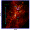 |
Fig. 15 NGC2264 as an example of StageIII: this is a HFS spanning ~10 pc, where IRS 1(above cone nebula) and IRS 2 (centre of spokes cluster) represent the two eyes of the hub shown by the green ellipse. |
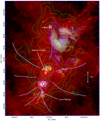 |
Fig. 16 Filaments of young stars in NGC2264: evidence that the filamentary structure of the gas clouds is inherited by the density distribution of young stars as shown by the green contours (tenth nearest neighbour density of cluster members catalogued by Sung et al. 2009). The violet line sketches mark these filaments of young stars. The hub has two centres of near-equal-intensity star formation with skewed evolutionary states. IRS1 is a ~10 M⊙ B2-type star well-known as Allen’s source, and sits above the cone nebula (a pillar irradiated by this star). IRS2 is the younger 150 L⊙ Class I type star surrounded by linearly aligned (in projection) young stars (Spokes cluster) detected at shorter than 70 μm. The YSOs in the Spokes-cluster display at least three distinct groups of radial velocities that may correspond to the filaments in which they formed. The colour-composite image is made by combining the images from the HOBYS survey (Motte et al. 2010), SPIRE 500 μm (red), PACS 70 μm (green), and MIPS 24 μm (blue) data. |
6.2 W40 in Aquila Rift: Stage IV
The W40 embedded cluster and HII region in the aquila rift has long been argued to be the result of star formation in a hub at the junctionof filaments by Mallick et al. (2013). These authors identified the young stellar population, and showed that the YSOs are located both in the central cluster and along the filaments. The filamentary structure is evident both in the gas and dust and also from the YSO density (see Fig. 4 of Mallick et al. 2013). However, these latter authors argued that the star formation took place in two epochs, one corresponding to the central cluster and the other in the filaments. In view of the HFS scenario, the population of young stars located in the filaments is predominantly a low-mass population that began well before the population that quickly formed the OB stellar cluster in the hub. This OB cluster has blown out the bipolar HII region as shown in Fig. 17. The scale bar of 1 pc shown in this figure assumes a distance of 436 pc to the region, considered to be the same to both W40 and Serpens South cluster (Ortiz-León et al. 2017).
Several features can be seen in Fig. 17. Both W40 and Serpens south clusters belong to the same network of filaments in the Aquila rift region, the W40 and Serpens south representing HFS in StageIV and StageII/III, respectively. W40 displays all the salient features of StageIV; the OB star formation represented by the OB cluster, the bipolar HII region created by the ionising radiation, and the effect of burning out the natal hub-composing filaments leading to the formation of pillar-like structures. Interestingly, the filamentary features that are likely swept up by the expanding HII bubble may also be represented by the 500 μm image, as marked in Fig. 17.
The W40 and Serpens-south regions display similarities with the IRS1 and IRS2 regions within NGC2264 in terms of evolutionarydifferences and physical separation. Given the lack of a fully blown HII region in NGC2264, it likely represents an earlier evolutionary stage, though one must consider the larger distance to NGC2264 and a denser network of filaments.
7 The hub-filament system compared with other models
Models aiming to describe high-mass star formation and cluster formation have always sought innovative ideas (e.g. Bonnell et al. 1998; Longmore et al. 2014; Kroupa et al. 2018) to coherently explain observational data. Global hierarchical collapse (GHC; Vázquez-Semadeni et al. 2019) and conveyor belt (CB; Longmore et al. 2014) models have recently found renewed interest, especially because of the observational support from longitudinal flows in filaments. These models, including the HFS model here, can derive support from several observational results. However, the mechanisms by which the result is obtained are different. Vázquez-Semadeni et al. (2019) claim that the GHC scenario is consistent with both the competitive accretion (Bonnell et al. 1998) and CB (Longmore et al. 2014) scenarios, but Krumholz & McKee (2020) argue that the CB model can better explain observational data sets of ONC and NGC6530. In contrast, these latter authors argue that the acceleration of star formation due to large-scale collapse (GHC) or a time-dependent increase in star formation efficiency are unable to explain the observed data.
While a detailed comparison of the HFS paradigm with these models is beyond the scope of this work, we highlight the major differences in the following.
-
Global hierarchical collapse represents a hierarchical collapse of the molecular cloud where collapse occurs within collapses, where the most massive structure collapses at the end, leading to acceleration of star formation. This scenario nicely reproduces the sequence of star formation whereby low-mass stars form prior to high-mass stars and the associated acceleration when high-mass star formation takes place. In the HFS, we assume a cloud that is filamentarily in structure and that there is no collapse over the cloud scale, and that the sequence of star formation is simply due to the HFS structure. Star formation in hubs (especially those with large networks of filaments) may mimic an acceleration owing to the quick amplification of densities resulting from overlapping filaments. Any analysis of star formation rates and efficiencies will require careful consideration of this density amplification mechanism and consequent longitudinal flows.
We envisage that the hub as an independent structure is likely to have more similarities with the GHC scenario. This is because the “two nodes of activity with an evolutionary skewness” within hubs is very frequently observed for which we do not have an explanation. These nodes are well represented by the BN/KL and Trapezium pair in Orion, and the IRS1 and IRS2 pair in NGC2264 described in the previous section. Such pairs are good representations of the GHC scenario.
The CB model predicts that the density of the hub remains roughly constant over many free-fall times, and any acceleration of star formation is the result of an increasing mass and not density. This is in contradiction to the result shown in Fig. 11, where the density increases in the hub from the pre-stellar to proto-stellar stages. The HFS scenario is primarily based on the density amplification of hubs and therefore differs from CB in that respect.
-
According to GHC, all massive clumps lead to massive star formation, whereas in the HFS paradigm, only those massive clumps that form junctions of large networks of filaments are conducive to the formation of massive stars. In the HFS,density amplification (with its associated mass increase) is responsible for massive star formation and not the sheer mass of the clump. Instead, we predict that the mass of the most massive star formed will be correlated with the network factor fnet =
 where
where  represent the number of filaments with a certain line mass
  . On thecontrary, GHC suggests a correlation between the most massive star and the clump mass which
Vázquez-Semadeni et al. (2019) claim to be represented by the known correlation of the most massive star with the cluster mass where it resides.
. On thecontrary, GHC suggests a correlation between the most massive star and the clump mass which
Vázquez-Semadeni et al. (2019) claim to be represented by the known correlation of the most massive star with the cluster mass where it resides. -
Longitudinal flows within filaments are representations of global infall in GHC moving towards a massive clump where high-mass stars form. In the CB model, they serve the purpose of mass transport which is similar to HFS. Vázquez-Semadeni et al. (2019) use the analogy of rivers from high altitudes to lakes to describe longitudinal flow. On the contrary, we have used the analogy of an electric current driven by a potential difference. In the HFS, longitudinal flows are best viewed as the current in a parallel electric circuit, where the currents in individual circuit paths add up at the source which is represented by the hub. According to HFS, detectable longitudinal flows (end-to-end) should be absent in isolated individual filaments with low-mass cores. Instead, such filaments may have flows directed towards cores located within them.
-
According to CB, the stars that form in the hub are those that remain as part of a bound cluster subsequent to gas dispersal. The HFS scenario here is different from CB in that respect. Because in the HFS scenario, the hub is where massive stars form, hubs evolve quickly, and therefore they likely result in relatively top-heavy mass functions. The lower mass stars and sub-stellar objects form slowly in the individual filaments, and a bound cluster should be the result of star formation in both the filaments and the hub. Observations of bound clusters clearly suggest a Salpeter-type mass function supporting the HFS scenario.
-
In the scenario of Kroupa et al. (2018), bursty star cluster formation is a result of incoming flows that are halted and restarted by an ionising feedback. This model also explains the origin of ejected O-stars. While these flows can be compared to longitudinal flows, the impact of feedback is unlikely to affect the inflow once a filamentary configuration (with a low volume filling factor) is considered. Formation of massive stars in a density-amplified hub implies an enhanced cross section for dynamical encounters and therefore ejections, similar to that discussed by Kroupa et al. (2018) and Oh et al. (2015).
The initial cluster formed in the hub may provide the necessary gravitational potential to dynamically influence the lower mass stars formed in the filaments in binding them to the cluster. It is also possible that the stars born in the filaments will move towards the hub because of the angular momentum imparted to the filaments at StageII of HFS. This is probably the most favoured scenario considering the swirling spiral-arm-like structure of HFS observed in MonR2 (Treviño-Morales et al. 2019).
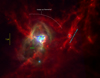 |
Fig. 17 W40 in the Aquila Rift as an example of StageIV: the formation of the W40 cluster in a hub has blown out the bipolar HII region (seen in blue-green; see Mallick et al. 2013, for details). The effects of radiation from OB stars “burning out” the hub-composing filaments can be seen as pillars. The ionising gas shock front sweeping up some filaments as it moves past it can also be seen. The colour composite uses Herschel SPIRE 500 μm image (tracing the filaments) as red, PACS 70 μm as green, and Spitzer MIPS 24 μm as blue. |
8 Discussion
8.1 A hierarchy of hub-filament systems
In this work we searched for hubs rather than filaments. Catalogues of filaments were produced using ATLASGAL (Li et al. 2013) and Hi-GAL (Schisano et al. 2020). A few caveats are associated with the present selection of HFS candidates, specifically the classification of HFS based on line-of-sight junctions; therefore, not all of the selected candidates are real junctions. A multi-wavelength comparison would be necessary for improved accuracy, especially by combining higher angular resolution data at shorter wavelengths contrasting the Herschel data used here. A non-negligible number of sources are located at distances beyond 8 kpc and up to 24 kpc. Given the uncertainties arising from the near–far distance confusion, sources with large distances should be viewed with extreme care, as they would result in very long filaments of between 50 and 150pc. Such filaments are not uncommon; indeed the giant molecular filaments or Galactic spines such as “Nessie” are similar in length or even longer (Goodman et al. 2014). The filaments constituting the hub sample display a peak at lengths between 10 and 20 pc; this is typical of giant molecular filaments (Li et al. 2013; Zucker et al. 2018). In the case of Galactic spines such as Nessie, the aspect ratios are very high (150–800). In the data analysed here, if we assumed one pixel as the width of the unresolved filaments, the lengths in pixels imply aspect ratios of 100–2000. Even though some of those high aspect ratios may be real, the uncertainties in the target distance combined with the coarse angular resolution (18′′) prompts extreme caution in viewing these aspect ratios.
Most nearby molecular clouds such as Taurus, Ophiucus, and Orion A and B are also elongated. If these clouds were to be placed far away at 3–5 kpc and viewed with Herschel, they would appear as giant filaments with lower aspect ratios (e.g. see Fig. 14 of Zucker et al. 2018), especially the Orion A and B clouds. The Trapezium cluster can then be viewed as the hub at the junction of Orion A and B clouds. In that sense, the filamentary structures, and consequently the HFSs found here, can represent (a) junctions of real giant molecular filaments with high aspect ratios, or (b) elongated clouds of low aspect ratio. When viewed at higher angular resolution (e.g. Mattern et al. 2018), the giant filaments and elongated clouds are likely to resolve themselves out into networks of further finer structures such as filaments with constant widths (Arzoumanian et al. 2011, 2019; Palmeirim et al. 2013) and/or velocity coherent fibres (Hacar et al. 2018). Therefore, elongated structures (with a range of aspect ratios) of dense gas in the cold ISM trace a hierarchy from the Milky Way bones/Galactic spines to elongated giant molecular clouds such as Orion, to individual filaments and fibres within them. It appears that junctions or HFSs can form at any level in this hierarchical distribution, even though one may naturally expect a lower frequency of HFSs at the bones and spines level.
How is this hierarchy in filaments and hubs related to the hierarchy of clouds, clumps, and cores? Observations show that most of the dense gas (Arzoumanian et al. 2019) within a molecular cloud is found in filaments of high aspect ratios. Giant molecular clouds such as Orion A and B are known to be elongated even from the earliest observations tracing the molecular gas in them (Bally et al. 1987). Elongated structures of dense gas such as filaments and fibres are yet to be placed in the context of the roundish molecular clouds and cores. However, the role of cylindrical and spherical geometries as distinct components composing the hierarchy is quite evident when viewing well-known targets such as Orion in the HFS scenario.
8.2 Massive discs and pre-stellar cores
Until now, there has been much emphasis on finding massive discs (Cesaroni et al. 2007) and massive pre-stellar cores (Motte et al. 2018a), both as part of an attempt to understand the conditions that lead to the formation of the highest mass stars such as those of 50–100 M⊙ or more massive objects. Both efforts have been largely unsuccessful, especially the search for pre-stellar cores. Subsequent to the arrival of ALMA, which provides the capacity to probe regions <1000 AU, searches for massive discs have resulted in an increased number of detections of Keplerian- (Sánchez-Monge et al. 2013; Johnston et al. 2015) or sub-Keplerian (Sanna et al. 2019)-type discs, but these are found around stars which are at best estimated to have a mass of 20 M⊙. Even though the term “massive stars” has been elusively employed in the literature, considering 8 M⊙ (set by free-fall time exceeding Kelvin-Helmholtz contraction time) or 20 M⊙ (Eddington ratio equal to one), the real quest is to understand the formation of the very-high-mass stars observationally catalogued in the Milky Way. In the HFS scenario for massive star formation discussed in Sect. 5, the above failures are perhaps expected. In the HFS scenario, the seeds of high-mass-star formation at the level of cores or proto-stellar fragments are not necessarily high in mass. Instead, they can be lower mass objects located inside a density-amplified hub, where both the accretion rates and the mass reservoir (in the HFS as a whole) are very high, as suggested by recent observations with ALMA (Chen et al. 2019; Treviño-Morales et al. 2019). This is, in general, counterintuitive and at odds with the expectations of searches made so far, where either a pre-stellar core with very high mass or a disc around an object with very high luminosity is searched for. Contrary to the failure of disc searches in the (sub)mm (Cesaroni et al. 2017), discs are found with a much higher frequency in infrared searches (Ilee et al. 2013) that employ CO-bandhead emission, finding Keplerian discs with much higher masses (35 M⊙ –55 M⊙). This result perhaps implies that well-developed disc structures may not form at earlier stages of accretion in massive stars, or if they do, only the inner regions (~100 AU) are Keplerian and the outer regions (~1000 AU) will be sub-Keplerian, as advocated by some numerical models (e.g. Kuiper et al. 2011). Indeed, a Keplerian disc is not favourable for mass accretion without the removal of angular momentum (see Sect. 8.3), and therefore near-spherical accretion onto a group of stars (as suggested by Eric Keto) fed by longitudinal flows is perhaps the mechanism by which the most massive stars form.
8.3 Formation of the most massive (≥100 M⊙) stars
The challenge in assembling ≥100 M⊙ stars is to not only in the need for a high disc accretion rate (~10−3 M⊙ yr−1), but also an envelope accretion rate and a sufficiently large massive reservoir, allowing the disc and envelope to be replenished as they feed the central star. Such a reservoir should be intact roughly until most of the stellar mass is assembled, withstanding the strong ionising radiation of the star. If the disc and envelope are themselves not replenished, helium ash will accumulate, and the star will move away to its death. In our scenario proposed in Sect. 5, the filaments provide a secondary reservoir, and the flattened hub acts as a large efficient disc where angular momentum is not an issue. The low volume filling factors of both filaments and hub allow large masses of dense gas to be channelled to the star in an efficient way. Subsequently, the hub will have an even more important role in the formation of the most massive stars, that is, in reducing fragmentation effects. Radiation feedback and magnetic fields are both thought to be crucial factors in controlling fragmentation as explained in Krumholz (2015, see Sect. 2.1). Magnetic fields inhibit fragmentation by inhibiting the formation of very thin and dense accretion discs, and so disc fragmentation does not occur. Instead, the disc slowly transports angular momentum outwards from the centre of the star via magnetic braking. This effect works smoothly over a larger physical scale, in contrast to radiative heating that has its influence only within ~1000 AU of the star. A flattened hub must be less dense than an accretion disc, but denser than the star forming clump, which when threaded by a magnetic field of average strength will provide stability against fragmentation while allowing mass transfer at high rates. This may be why flattened toroidal structures are more commonly found than Keplerian discs in sub-mm studies of high-mass star formation (e.g. Beltrán et al. 2011). Therefore, it appears that in forming the most massive stars, there is a three-step process in mass transfer, from filaments to hubs to envelopes/discs; whereas low-mass stars can form easily without the hub, for example from filament fragmentation.
A magnetically threaded hub (of size ~0.5 pc) can lead to locally (~100 AU) high field strengths close to the star by simply considering frozen-in-field. For example, in the case of NGC2264 discussed in Sect. 6.1, the CN Zeeman observations of the hub region of NGC2264-C (IRS1) indicate marginal support (Maury et al. 2012) at the large scale. At smaller scales, observations of IRS1 show that the star is highly magnetic and spotted, implying a stronger field close to the star (Fossati et al. 2014). Similarly, a strong magnetic field (~100 μG) is estimated around IRS2 (Kwon et al. 2011), in support of the role of magnetic fields in the formation of massive stars in the NGC2264 hub. Fossil fields from star formation are suggested as the main mechanism to explain strong and ordered magnetic fields in massive stars (Walder et al. 2012). Massive stars cannot be spun down to the values observed on the main-sequence without having long disc lifetimes or a high magnetic field strength as argued by Rosen et al. (2012). As we pointed out in Sect. 8.2, the low rate of detection of discs at earlier evolutionary stages may imply that magnetic fields are stronger in the central regions of the hub where the massive star forms. Hence, our result that all massive stars form in hubs should not be surprising.
If accretion proceeds in this three-step process and a hole is punched out by the stellar radiation in the inner ~100–1000 AU regions, the accretion flows close to the star and/or in the disc will naturally become strongly ionised (Keto 2002, 2003; Keto & Wood 2006). Evidence that ionised gas flows play a significant role is suggested by the Brα line observations of sources in M17 (Blum et al. 2004). How much mass a star can gain via ionised accretion flows remains to be understood, especially accounting for simultaneous mass loss via stellar winds. This may be key to understanding the formation of the monstrous stars found in the Milky Way, often as optically visible stars enshrouded by thick envelopes.
8.4 Feedback and triggered star formation
Thanks to the Spitzer Space Telescope, bubbles have attracted much attention, and the Milky Way disc was dubbed a bubbling disc by Churchwell et al. (2006). Bubbles have been the preferred observational targets to examine therole of feedback and its ability to trigger star formation (Deharveng et al. 2010; Palmeirim et al. 2017; Samal et al. 2018) and specifically massive stars (Zavagno et al. 2007). Palmeirim et al. (2017) find that ~23% of the Hi-GAL clumps are located in the direction of the bubbles and Deharveng et al. (2010) find that 86% of the bubbles contain ionised gas. These observations have also renewed interest in models of triggered star formation (Walch et al. 2015; Deharveng et al. 2010), exploring them as a mechanism for high-mass star formation. The HFS candidate catalogue presented here includes many clumps that are located on the rim or edge of bubbles and also represent a hub. Therefore, even when massive star formation takes place at the edges of bubbles, our results suggest thatit happens within a junction of three or more filamentary features located on the bubble surfaces. Moreover, bubbles come in a variety of sizes from a few to 10–15 pc. The driving sources can be early B-type stars, young O-stars, or supernovae, implying a large range in the energy budget involved. In view of the HFS scenario presented here, we caution that not all bubbles are real bubbles formed by swept up gas. In particular, a vast majority of dense gas found in bipolar bubbles (Samal et al. 2018) may be simply confused with the hub-composing filaments.
Triggering as a mechanism to form massive stars or simply groups of stars should be examined with caution, accounting carefully for the energy budget of the driving factors and the efficiency of the resulting star formation. Indeed, Deharveng et al. (2010) point out that only a few large bubbles (size ≥ 15 pc) are candidates for triggered star formation, in which case the driving source is often a supernova. Lower energy processes of “sweeping” produced by B-stars may enhance the formation of HFS or filaments, but not essentially “trigger” more efficient starformation. Considering the sheer volume filling factor of filaments in a molecular cloud, much of the feedback energy can escape through inter-filamentary voids (Sect. 5: StageIII, IV; Dale & Bonnell 2011), while the dust-processed radiation and ionised gas pressure helps to form and sweep the HII shells (Lopez et al. 2014) without having much effect on triggering further star formation. Indeed, Rosen et al. (2014) find that none of the known energy loss channels can successfully explain more than a small fraction of the energy injected by massive stars in stellar clusters. This implies that most of that energy is lost through inter-filamentary voids. Swept up gas in bubbles and shells enhances the formation of HFSs, which in turn allow massive star formation to take place.
8.5 Caveats and future work
The main caveat of this observational exercise is the relatively poor resolution of the data used to trace the HFSs. The data is sensitive only to the most massive and nearby filaments. Next, the identified candidates are limited by the extent of the Hi-GAL release made by the clumps catalogue of Elia et al. (2017), and the limitations in the distance estimates. We foresee that a catalogue of clumps with wider coverage and better distance estimates will be available soon that will lead to better HFS identification. Identification of filaments can ideally be done in two bands with different resolution, especially employing the PACS 160 μm band that would allow the superior spatial resolution to be exploited in order to better resolve the HFS structure.
While our paradigm is the result of an attempt to coherently place several observational facts into context, the observational results used to justify the paradigm were not made to test the paradigm. Building upon the vast amount of high-quality data produced by large-scale surveys, further multi-wavelength studies of both the stars and gas simultaneously are required to test the HFS paradigm. Such observations should be planned to carefully distinguish features that would emerge in three main scenarios of cluster formation, namely (a) the HFS paradigm presented here, (b) GHC, and (c) the CB model. As we argue in Sect. 7, even though all three scenarios attempt to explain the known properties of young clusters and giant molecular clouds, one can expect to observe specific differences between the models. One of these is the magnitude and importance of longitudinal flows in isolated filaments versus HFSs. The role of the magnetic field support in the filaments and hubs, especially at smaller physical scales, is also a crucial factor to investigate.
9 Summary and conclusions
We searched for candidate HFSs in the Milky Way inner disc by searching for filamentary structures around 35 000 clumps in the Hi-GAL catalogue detected at 3σ and above in at least four bands. DisPerSE software was used to accomplish this on 10′ × 10′ cut-outs of 250 μm images centred on each target clump. A hub is defined as a junction of three or more filaments on the clump, where each filament has a minimum length of 55′′ (3 × FWHM of the 250 μm beam), at least 18′′ (one beam) of which residing within the FWHM of the clump.
-
Of the 34575 clumps examined, 3703 (~11%) are HFS candidates, of which ~2150 (60%) are pre-stellar and ~1400 (40%) are proto-stellar. We find that 144 clumps are saturated in one or more of the Herschel bands, all of which are proto-stellar in nature and are among the most active sites of star formation.
-
There are 26 135 non-hub clumps, of which 10 380 are located at the junction of two filamentary skeletons and 15 755 form thetip of a single filament. We find that 4736 clumps are not associated with any filaments.
-
Filaments in the HFS sample are represented by mean lengths of ~10–20pc, masses of ~5 × 10⁴ M⊙, and line masses (M/L) of ~2 × 10³ M⊙ pc−1. Filaments found around non-hub clumps have mean lengths of ~8 pc and masses of ~104 M⊙.
-
Circularly averaged radial density profiles of all hub and non-hub clumps show that the column density of the hubs is enhanced by a factor of approximately two in pre-stellar and average proto-stellar sources, shooting up to a factor of aboutten in the saturated proto-stellar sources.
-
All clumps with a luminosity L ≥ 105 L⊙ located within 5 kpc and L ≥ 104 L⊙ located within 2 kpc are HFSs. Clumps at distances ≥10 kpc are generally classified as non-hubs due to insufficient angular resolution to resolve the structure. This shows that all massive-star formation takes place in HFSs.
We propose a filaments to clusters paradigm for star formation based on the results above.
-
Flow-driven filaments driven by intra-cloud velocity dispersion or by external factors collide to form hubs. Because the junction happens with an offset to the centre of mass, the hub gains a small twist acquiring an initial angular momentum. The hub will have a flattened geometry, more likely an oblate spheroid with two gravitational centres.
-
Gravitational collapse of the hub may be delayed considering the relaxation time necessary for an object formed via collision of filaments. The hub begins collapsing at one of the two gravitational centres, followed by the collapse of the remaining centre. The enhanced density and mass of the hub provide conditions to form massive stars.
-
Hubs can trigger and drive longitudinal flows within filaments, the mass flow from which will not only bring additional mass to the hub, but can also replenish the reservoir in the hub as star formation proceeds. The radiation, ionised gas, and stellar wind pressures are beamed out to inter-filamentary voids by punching holes in the flattened hub, minimising the effects of feedback.
-
A magnetically threaded hub offers stability against fragmentation, favouring the formation of a group of OB stars. Because hubs are centrally located in HFSs, this effect naturally results in mass segregation. The ionised gas escaping on either face of the flattened hub results in bipolar HII regions, slowly destroying the filaments. Filament tips burnt up by radiation and ionisation fronts can cause the pillars of creation.
-
The net result of star formation in a HFS is a mass-segregated young stellar cluster, where the low-mass stars form slowly over 106 yr in the individual filaments, starting even before the hub formation, and high-mass stars form in the hub quickly in 105 yr. The resulting mass function is a sum of filament and hub (top heavy) mass functions.
-
A hub that becomes gravitationally unstable before the filaments can produce a cluster of low-mass stars will preferentially lead to the formation of isolated OB associations.
We compared the proposed HFS paradigm with observational studies in the literature of two nearby well-known regions of star formation, namely NGC 2264 and W40.
-
NGC 2264 represents StageIII of the paradigm. We show that previously unpublished Herschel SPIRE data from the archive display a spectacular network of filaments feeding the NGC 2264 region that represents a hub. The hub is composed of IRS1 (Allen source) and the Spokes cluster around IRS2. These two represent the two nodes within an oblate spheroidal hub where IRS2 is younger than the IRS1 region and displays the evolutionary skewness of star formation in hubs represented by StageIII.
-
We produce tenth nearest neighbour young stellar density maps using membership data from the literature. The NN maps also show filamentary structures merging at the hubs, and therefore the YSOs have not had the time to erase the structure inherited from its natal filaments. This result is further supported at the hub level as represented by the Spokes cluster that was previously claimed to represent primordial structure.
-
W40 displays all the characteristic features of StageIV of the HFS paradigm. The W40 cluster has formed in a hub that is at the junction of three to four main filaments. The hub is known to have OB stellar content that has driven a bipolar HII region that appears to have swept up other lower density filaments in the northern boundary. The main filaments display pillar-like tips as the radiation from the W40 cluster has destroyed the molecular material. We assembled a spectacular wide-field colour composite image to highlight these salient features.
Acknowledgements
M.S.N.K. acknowledges the support from FCT – Fundação para a Ciência e a Tecnologia through Investigadorcontracts and exploratory project (IF/00956/2015/CP1273/CT0002). D.A. and P.P. acknowledge support from FCT/MCTES through Portuguese national funds (PIDDAC) by grant UID/FIS/04434/2019. P.P. receives support from fellowship SFRH/BPD/110176/2015 funded by FCT (Portugal) and POPH/FSE (EC). Herschel Hi-GAL data processing, map production, and source catalog generation is the result of a multi-year effort that was initially funded thanks to Contracts I/038/080/0and I/029/12/0 from ASI, Agenzia Spaziale Italiana. Herschel is an ESA space observatory with science instruments provided by European-led Principal Investigator consortia and with important participation from NASA. Thiswork is based on observations obtained with Herschel-PACS and Herschel-SPIRE photometers. PACS has been developed by a consortium of institutes led by MPE (Germany) and including UVIE (Austria); KU Leuven, CSL, IMEC (Belgium); CEA, LAM (France); MPIA (Germany); INAF-IFSI/OAA/OAP/OAT, LENS, SISSA (Italy); IAC (Spain). This development has been supported by the funding agencies BMVIT (Austria), ESA-PRODEX (Belgium), CEA/CNES (France), DLR (Germany), ASI/INAF (Italy),and CICYT/MCYT (Spain). SPIRE has been developed by a consortium of institutes led by CardiffUniv. (UK) and including: Univ. Lethbridge (Canada);NAOC (China); CEA, LAM (France); IFSI, Univ. Padua (Italy); IAC (Spain);Stockholm Observatory (Sweden); Imperial College London, RAL, UCL-MSSL, UKATC, Univ. Sussex (UK); and Caltech, JPL, NHSC, Univ. Colorado(USA). This development has been supported by national funding agencies: CSA(Canada); NAOC (China); CEA, CNES, CNRS (France); ASI (Italy); MCINN(Spain); SNSB (Sweden); STFC, UKSA (UK); and NASA (USA).
References
- André, P., Men’shchikov, A., Bontemps, S., et al. 2010, A&A, 518, L102 [NASA ADS] [CrossRef] [EDP Sciences] [Google Scholar]
- André, P., Di Francesco, J., Ward-Thompson, D., et al. 2014, Protostars and Planets VI, eds. H. Beuther, R. S. Klessen, C. P. Dullemond, & T. Henning (Tucson: University of Arizona Press), 27 [Google Scholar]
- Arzoumanian, D., André, P., Didelon, P., et al. 2011, A&A, 529, L6 [Google Scholar]
- Arzoumanian, D., André, P., Könyves, V., et al. 2019, A&A, 621, A42 [NASA ADS] [CrossRef] [EDP Sciences] [Google Scholar]
- Bally, J., Langer, W. D., Stark, A. A., & Wilson, R. W. 1987, ApJ, 312, L45 [NASA ADS] [CrossRef] [Google Scholar]
- Baug, T., Dewangan, L. K., Ojha, D. K., et al. 2018, ApJ, 852, 119 [CrossRef] [Google Scholar]
- Behrend, R., & Maeder, A. 2001, A&A, 373, 190 [NASA ADS] [CrossRef] [EDP Sciences] [Google Scholar]
- Beltrán, M. T., Cesaroni, R., Neri, R., & Codella, C. 2011, A&A, 525, A151 [NASA ADS] [CrossRef] [EDP Sciences] [Google Scholar]
- Beltrán, M. T., Padovani, M., Girart, J. M., et al. 2019, A&A, 630, A54 [CrossRef] [EDP Sciences] [Google Scholar]
- Blum, R. D., Barbosa, C. L., Damineli, A., Conti, P. S., & Ridgway, S. 2004, ApJ, 617, 1167 [NASA ADS] [CrossRef] [Google Scholar]
- Bonnell, I. A., Bate, M. R., & Zinnecker, H. 1998, MNRAS, 298, 93 [NASA ADS] [CrossRef] [Google Scholar]
- Buckle, J. V., & Richer, J. S. 2015, MNRAS, 453, 2006 [CrossRef] [Google Scholar]
- Buckle, J. V., Richer, J. S., & Davis, C. J. 2012, MNRAS, 423, 1127 [NASA ADS] [CrossRef] [Google Scholar]
- Cesaroni, R., Galli, D., Lodato, G., Walmsley, C. M., & Zhang, Q. 2007, in Protostars and Planets V, eds. B. Reipurth, D. Jewitt, & K. Keil (Tucson, AZ: UNiversity of Arizona Press), 197 [Google Scholar]
- Cesaroni, R., Sánchez-Monge, Á., Beltrán, M. T., et al. 2017, A&A, 602, A59 [NASA ADS] [CrossRef] [EDP Sciences] [Google Scholar]
- Chen, H.-R. V., Zhang, Q., Wright, M. C. H., et al. 2019, ApJ, 875, 24 [NASA ADS] [CrossRef] [Google Scholar]
- Churchwell, E., Povich, M. S., Allen, D., et al. 2006, ApJ, 649, 759 [NASA ADS] [CrossRef] [Google Scholar]
- Crowther, P. A., Schnurr, O., Hirschi, R., et al. 2010, MNRAS, 408, 731 [NASA ADS] [CrossRef] [Google Scholar]
- Dale, J. E., & Bonnell, I. 2011, MNRAS, 414, 321 [NASA ADS] [CrossRef] [Google Scholar]
- Deharveng, L., Schuller, F., Anderson, L. D., et al. 2010, A&A, 523, A6 [NASA ADS] [CrossRef] [EDP Sciences] [Google Scholar]
- Deharveng, L., Zavagno, A., Samal, M. R., et al. 2015, A&A, 582, A1 [NASA ADS] [CrossRef] [EDP Sciences] [Google Scholar]
- Dewangan, L. K., Ojha, D. K., & Baug, T. 2017, ApJ, 844, 15 [CrossRef] [Google Scholar]
- Elia, D., Molinari, S., Schisano, E., et al. 2017, MNRAS, 471, 100 [NASA ADS] [CrossRef] [Google Scholar]
- Eswaraiah, C., Lai, S.-P., Chen, W.-P., et al. 2017, ApJ, 850, 195 [NASA ADS] [CrossRef] [Google Scholar]
- Fossati, L., Zwintz, K., Castro, N., et al. 2014, A&A, 562, A143 [NASA ADS] [CrossRef] [EDP Sciences] [Google Scholar]
- Fukui, Y., Ohama, A., Hanaoka, N., et al. 2014, ApJ, 780, 36 [NASA ADS] [CrossRef] [Google Scholar]
- González, M., & Alfaro, E. J. 2017, MNRAS, 465, 1889 [NASA ADS] [CrossRef] [Google Scholar]
- Goodman, A. A., Alves, J., Beaumont, C. N., et al. 2014, ApJ, 797, 53 [NASA ADS] [CrossRef] [Google Scholar]
- Grellmann, R., Ratzka, T., Kraus, S., et al. 2011, A&A, 532, A109 [NASA ADS] [CrossRef] [EDP Sciences] [Google Scholar]
- Griffin, M. J., Abergel, A., Abreu, A., et al. 2010, A&A, 518, L3 [Google Scholar]
- Hacar, A., Tafalla, M., Forbrich, J., et al. 2018, A&A, 610, A77 [NASA ADS] [CrossRef] [EDP Sciences] [Google Scholar]
- Heiles, C. 1979, ApJ, 229, 533 [NASA ADS] [CrossRef] [Google Scholar]
- Henshaw, J. D., Jiménez-Serra, I., Longmore, S. N., et al. 2017, MNRAS, 464, L31 [NASA ADS] [CrossRef] [Google Scholar]
- Herbig, G. H. 1954, ApJ, 119, 483 [NASA ADS] [CrossRef] [Google Scholar]
- Hillenbrand, L. A., & Hartmann, L. W. 1998, ApJ, 492, 540 [NASA ADS] [CrossRef] [Google Scholar]
- Ilee, J. D., Wheelwright, H. E., Oudmaijer, R. D., et al. 2013, MNRAS, 429, 2960 [NASA ADS] [CrossRef] [Google Scholar]
- Inoue, T., & Fukui, Y. 2013, ApJ, 774, L31 [NASA ADS] [CrossRef] [Google Scholar]
- Inoue, T., Hennebelle, P., Fukui, Y., et al. 2018, PASJ, 70, S53 [NASA ADS] [Google Scholar]
- Inutsuka, S.-i., Inoue, T., Iwasaki, K., & Hosokawa, T. 2015, A&A, 580, A49 [NASA ADS] [CrossRef] [EDP Sciences] [Google Scholar]
- Johnston, K. G., Robitaille, T. P., Beuther, H., et al. 2015, ApJ, 813, L19 [NASA ADS] [CrossRef] [Google Scholar]
- Kainulainen, J., Stutz, A. M., Stanke, T., et al. 2017, A&A, 600, A141 [NASA ADS] [CrossRef] [EDP Sciences] [Google Scholar]
- Kennicutt, R. C., & Evans, N. J. 2012, ARA&A, 50, 531 [NASA ADS] [CrossRef] [Google Scholar]
- Keto, E. 2002, ApJ, 568, 754 [NASA ADS] [CrossRef] [Google Scholar]
- Keto, E. 2003, ApJ, 599, 1196 [NASA ADS] [CrossRef] [Google Scholar]
- Keto, E., & Wood, K. 2006, ApJ, 637, 850 [NASA ADS] [CrossRef] [Google Scholar]
- Könyves, V., André, P., Men’shchikov, A., et al. 2015, A&A, 584, A91 [NASA ADS] [CrossRef] [EDP Sciences] [Google Scholar]
- Könyves, V., Andre, P., Arzoumanian, D., et al. 2019, A&A, 635, A34 [Google Scholar]
- Kroupa, P., Jeřábková, T., Dinnbier, F., Beccari, G., & Yan, Z. 2018, A&A, 612, A74 [NASA ADS] [CrossRef] [EDP Sciences] [Google Scholar]
- Krumholz, M. R. 2006, ApJ, 641, L45 [NASA ADS] [CrossRef] [Google Scholar]
- Krumholz, M. R. 2015, Astrophys. Space Sci. Lib., 412, 43 [NASA ADS] [CrossRef] [Google Scholar]
- Krumholz, M. R., & McKee, C. F. 2020, MNRAS, 494, 624 [NASA ADS] [CrossRef] [Google Scholar]
- Krumholz, M. R., Klein, R. I., McKee, C. F., Offner, S. S. R., & Cunningham, A. J. 2009, Science, 323, 754 [NASA ADS] [CrossRef] [PubMed] [Google Scholar]
- Krumholz, M. R., McKee, C. F., & Bland -Hawthorn, J. 2019, ARA&A, 57, 227 [NASA ADS] [CrossRef] [Google Scholar]
- Kuiper, R., Klahr, H., Beuther, H., & Henning, T. 2011, ApJ, 732, 20 [NASA ADS] [CrossRef] [Google Scholar]
- Kumar, M. S. N., & Grave, J. M. C. 2007, A&A, 472, 155 [NASA ADS] [CrossRef] [EDP Sciences] [Google Scholar]
- Kumar, M. S. N., Tafalla, M., & Bachiller, R. 2004, A&A, 426, 195 [CrossRef] [EDP Sciences] [Google Scholar]
- Kumar, M. S. N., Keto, E., & Clerkin, E. 2006, A&A, 449, 1033 [NASA ADS] [CrossRef] [EDP Sciences] [Google Scholar]
- Kumar, M. S. N., Davis, C. J., Grave, J. M. C., Ferreira, B., & Froebrich, D. 2007, MNRAS, 374, 54 [NASA ADS] [CrossRef] [Google Scholar]
- Kumar, M. S. N., Contreras Peña, C., Lucas, P. W., & Thompson, M. A. 2016, ApJ, 833, 24 [NASA ADS] [CrossRef] [Google Scholar]
- Kwon, J., Tamura, M., Kandori, R., et al. 2011, ApJ, 741, 35 [NASA ADS] [CrossRef] [Google Scholar]
- Lada, C. J., & Lada, E. A. 2003, ARA&A, 41, 57 [NASA ADS] [CrossRef] [Google Scholar]
- Lada, C. J., Lombardi, M., & Alves, J. F. 2010, ApJ, 724, 687 [NASA ADS] [CrossRef] [Google Scholar]
- Li, G.-X., Wyrowski, F., Menten, K., & Belloche, A. 2013, A&A, 559, A34 [NASA ADS] [CrossRef] [EDP Sciences] [Google Scholar]
- Li, G.-X., Urquhart, J. S., Leurini, S., et al. 2016, A&A, 591, A5 [NASA ADS] [CrossRef] [EDP Sciences] [Google Scholar]
- Liu, H. B., Jiménez-Serra, I., Ho, P. T. P., et al. 2012, ApJ, 756, 10 [NASA ADS] [CrossRef] [Google Scholar]
- Longmore, S. N., Kruijssen, J. M. D., Bastian, N., et al. 2014, in Protostars and Planets VI, eds. H. Beuther, R. S. Klessen, C. P. Dullemond, & T. Henning (Tucson, AZ: University of Arizona Press), 291 [Google Scholar]
- Lopez, L. A., Krumholz, M. R., Bolatto, A. D., et al. 2014, ApJ, 795, 121 [NASA ADS] [CrossRef] [Google Scholar]
- Maíz Apellániz, J. 2019, A&A, 630, A119 [NASA ADS] [CrossRef] [EDP Sciences] [Google Scholar]
- Mallick, K. K., Kumar, M. S. N., Ojha, D. K., et al. 2013, ApJ, 779, 113 [NASA ADS] [CrossRef] [Google Scholar]
- Mattern, M., Kauffmann, J., Csengeri, T., et al. 2018, A&A, 619, A166 [NASA ADS] [CrossRef] [EDP Sciences] [Google Scholar]
- Maury, A. J., Wiesemeyer, H., & Thum, C. 2012, A&A, 544, A69 [NASA ADS] [CrossRef] [EDP Sciences] [Google Scholar]
- McKee, C. F., & Ostriker, E. C. 2007, ARA&A, 45, 565 [NASA ADS] [CrossRef] [Google Scholar]
- McKee, C. F., & Tan, J. C. 2003, ApJ, 585, 850 [NASA ADS] [CrossRef] [MathSciNet] [Google Scholar]
- Molinari, S., Swinyard, B., Bally, J., et al. 2010, A&A, 518, L100 [NASA ADS] [CrossRef] [EDP Sciences] [Google Scholar]
- Molinari, S., Schisano, E., Faustini, F., et al. 2011, A&A, 530, A133 [NASA ADS] [CrossRef] [EDP Sciences] [Google Scholar]
- Molinari, S., Schisano, E., Elia, D., et al. 2016, A&A, 591, A149 [NASA ADS] [CrossRef] [EDP Sciences] [Google Scholar]
- Montillaud, J., Juvela, M., Vastel, C., et al. 2019, A&A, 631, A3 [NASA ADS] [CrossRef] [EDP Sciences] [Google Scholar]
- Motte, F., Zavagno, A., Bontemps, S., et al. 2010, A&A, 518, L77 [NASA ADS] [CrossRef] [EDP Sciences] [Google Scholar]
- Motte, F., Bontemps, S., & Louvet, F. 2018a, ARA&A, 56, 41 [NASA ADS] [CrossRef] [Google Scholar]
- Motte, F., Nony, T., Louvet, F., et al. 2018b, Nat. Astron., 2, 478 [NASA ADS] [CrossRef] [Google Scholar]
- Muench, A. A., Lada, E. A., Lada, C. J., & Alves, J. 2002, ApJ, 573, 366 [NASA ADS] [CrossRef] [Google Scholar]
- Myers, P. C. 2009, ApJ, 700, 1609 [NASA ADS] [CrossRef] [EDP Sciences] [Google Scholar]
- Myers, A. T., McKee, C. F., Cunningham, A. J., Klein, R. I., & Krumholz, M. R. 2013, ApJ, 766, 97 [NASA ADS] [CrossRef] [Google Scholar]
- Oh, S., Kroupa, P., & Pflamm-Altenburg, J. 2015, ApJ, 805, 92 [NASA ADS] [CrossRef] [Google Scholar]
- Ojha, D. K., Kumar, M. S. N., Davis, C. J., & Grave, J. M. C. 2010, MNRAS, 407, 1807 [NASA ADS] [CrossRef] [Google Scholar]
- Ortiz-León, G. N., Dzib, S. A., Kounkel, M. A., et al. 2017, ApJ, 834, 143 [NASA ADS] [CrossRef] [Google Scholar]
- Palla, F., Randich, S., Pavlenko, Y. V., Flaccomio, E., & Pallavicini, R. 2007, ApJ, 659, L41 [NASA ADS] [CrossRef] [Google Scholar]
- Palmeirim, P., André, P., Kirk, J., et al. 2013, A&A, 550, A38 [NASA ADS] [CrossRef] [EDP Sciences] [Google Scholar]
- Palmeirim, P., Zavagno, A., Elia, D., et al. 2017, A&A, 605, A35 [NASA ADS] [CrossRef] [EDP Sciences] [Google Scholar]
- Pavlík, V., Kroupa, P., & Šubr, L. 2019, A&A, 626, A79 [CrossRef] [EDP Sciences] [Google Scholar]
- Peretto, N., André, P., & Belloche, A. 2006, A&A, 445, 979 [NASA ADS] [CrossRef] [EDP Sciences] [Google Scholar]
- Peretto, N., Fuller, G. A., Duarte-Cabral, A., et al. 2013, A&A, 555, A112 [NASA ADS] [CrossRef] [EDP Sciences] [Google Scholar]
- Peretto, N., Fuller, G. A., André, P., et al. 2014, A&A, 561, A83 [NASA ADS] [CrossRef] [EDP Sciences] [Google Scholar]
- Peters, T., Klessen, R. S., Mac Low, M.-M., & Banerjee, R. 2010, ApJ, 725, 134 [NASA ADS] [CrossRef] [Google Scholar]
- Poglitsch, A., Waelkens, C., Geis, N., et al. 2010, A&A, 518, L2 [NASA ADS] [CrossRef] [EDP Sciences] [Google Scholar]
- Portegies Zwart, S. F., McMillan, S. L. W., & Gieles, M. 2010, ARA&A, 48, 431 [NASA ADS] [CrossRef] [Google Scholar]
- Povich, M. S., & Whitney, B. A. 2010, ApJ, 714, L285 [NASA ADS] [CrossRef] [Google Scholar]
- Reggiani, M., Robberto, M., Da Rio, N., et al. 2011, A&A, 534, A83 [NASA ADS] [CrossRef] [EDP Sciences] [Google Scholar]
- Rosen, A. L., Krumholz, M. R., & Ramirez-Ruiz, E. 2012, ApJ, 748, 97 [NASA ADS] [CrossRef] [Google Scholar]
- Rosen, A. L., Lopez, L. A., Krumholz, M. R., & Ramirez-Ruiz, E. 2014, MNRAS, 442, 2701 [NASA ADS] [CrossRef] [Google Scholar]
- Roy, A., André, P., Arzoumanian, D., et al. 2019, A&A, 626, A76 [NASA ADS] [CrossRef] [EDP Sciences] [Google Scholar]
- Samal, M. R., Deharveng, L., Zavagno, A., et al. 2018, A&A, 617, A67 [NASA ADS] [CrossRef] [EDP Sciences] [Google Scholar]
- Sánchez-Monge, Á., Cesaroni, R., Beltrán, M. T., et al. 2013, A&A, 552, L10 [NASA ADS] [CrossRef] [EDP Sciences] [Google Scholar]
- Sanna, A., Kölligan, A., Moscadelli, L., et al. 2019, A&A, 623, A77 [NASA ADS] [CrossRef] [EDP Sciences] [Google Scholar]
- Sano, H., Enokiya, R., Hayashi, K., et al. 2018, PASJ, 70, S43 [NASA ADS] [CrossRef] [Google Scholar]
- Schisano, E., Molinari, S., Elia, D., et al. 2020, MNRAS, 492, 5420 [NASA ADS] [CrossRef] [Google Scholar]
- Schmeja, S., Kumar, M. S. N., & Ferreira, B. 2008, MNRAS, 389, 1209 [NASA ADS] [CrossRef] [Google Scholar]
- Schneider, S., & Elmegreen, B. G. 1979, ApJS, 41, 87 [NASA ADS] [CrossRef] [Google Scholar]
- Schneider, N., Csengeri, T., Hennemann, M., et al. 2012, A&A, 540, L11 [NASA ADS] [CrossRef] [EDP Sciences] [Google Scholar]
- Shepherd, D. S., & Churchwell, E. 1996, ApJ, 472, 225 [NASA ADS] [CrossRef] [Google Scholar]
- Shimajiri, Y., André, P., Ntormousi, E., et al. 2019, A&A, 632, A83 [NASA ADS] [CrossRef] [EDP Sciences] [Google Scholar]
- Smith, N. 2006, MNRAS, 367, 763 [NASA ADS] [CrossRef] [Google Scholar]
- Sousbie, T. 2011, MNRAS, 414, 350 [NASA ADS] [CrossRef] [Google Scholar]
- Sung, H., Stauffer, J. R., & Bessell, M. S. 2009, AJ, 138, 1116 [NASA ADS] [CrossRef] [Google Scholar]
- Teixeira, P. S. 2008, PhD thesis, Harvard-Smithsonian Center for Astrophysics, USA; University of Lisbon, Portugal [Google Scholar]
- Teixeira, P. S., Lada, C. J., Young, E. T., et al. 2006, ApJ, 636, L45 [NASA ADS] [CrossRef] [Google Scholar]
- Tobin, J. J., Hartmann, L., Fűrész, G., Hsu, W.-H., & Mateo, M. 2015, AJ, 149, 119 [NASA ADS] [CrossRef] [Google Scholar]
- Torii, K., Hasegawa, K., Hattori, Y., et al. 2015, ApJ, 806, 7 [NASA ADS] [CrossRef] [Google Scholar]
- Traficante, A., Calzoletti, L., Veneziani, M., et al. 2011, MNRAS, 416, 2932 [NASA ADS] [CrossRef] [Google Scholar]
- Traficante, A., Fuller, G. A., Duarte-Cabral, A., et al. 2020, MNRAS, 491, 4310 [NASA ADS] [CrossRef] [Google Scholar]
- Treviño-Morales, S. P., Fuente, A., Sánchez-Monge, Á., et al. 2019, A&A, 629, A81 [NASA ADS] [CrossRef] [EDP Sciences] [Google Scholar]
- Urquhart, J. S., König, C., Giannetti, A., et al. 2018, MNRAS, 473, 1059 [NASA ADS] [CrossRef] [Google Scholar]
- Vázquez-Semadeni, E., Gómez, G. C., Jappsen, A. K., et al. 2007, ApJ, 657, 870 [NASA ADS] [CrossRef] [Google Scholar]
- Vázquez-Semadeni, E., Palau, A., Ballesteros-Paredes, J., Gómez, G. C., & Zamora-Avilés, M. 2019, MNRAS, 490, 3061 [NASA ADS] [CrossRef] [Google Scholar]
- Walch, S., Whitworth, A. P., Bisbas, T. G., Hubber, D. A., & Wünsch, R. 2015, MNRAS, 452, 2794 [NASA ADS] [CrossRef] [Google Scholar]
- Walder, R., Folini, D., & Meynet, G. 2012, Space Sci. Rev., 166, 145 [NASA ADS] [CrossRef] [Google Scholar]
- Walker, M. F. 1956, ApJS, 2, 365 [NASA ADS] [CrossRef] [Google Scholar]
- Wang, J.-W., Lai, S.-P., Eswaraiah, C., et al. 2019, ApJ, 876, 42 [NASA ADS] [CrossRef] [Google Scholar]
- Ward, J. L., Kruijssen, J. M. D., & Rix, H.-W. 2019, MNRAS, 495, 663 [Google Scholar]
- Whitworth, A.P., Bhattal, A. S., Chapman, S. J., Disney, M. J., & Turner, J. A. 1994, MNRAS, 268, 291 [NASA ADS] [CrossRef] [Google Scholar]
- Whitworth, A., Lomax, O., Balfour, S., et al. 2018, PASJ, 70, S55 [NASA ADS] [CrossRef] [Google Scholar]
- Williams, G. M., Peretto, N., Avison, A., Duarte-Cabral, A., & Fuller, G. A. 2018, A&A, 613, A11 [NASA ADS] [CrossRef] [EDP Sciences] [Google Scholar]
- Zapata, L. A., Garay, G., Palau, A., et al. 2019, ApJ, 872, 176 [NASA ADS] [CrossRef] [Google Scholar]
- Zavagno, A., Pomarès, M., Deharveng, L., et al. 2007, A&A, 472, 835 [NASA ADS] [CrossRef] [EDP Sciences] [Google Scholar]
- Zucker, C., Battersby, C., & Goodman, A. 2018, ApJ, 864, 153 [NASA ADS] [CrossRef] [Google Scholar]
All Tables
All Figures
|
Fig. 1 Pixel value distribution histogram examples of 10′ × 10′ cut-out maps of (A) Background-dominated image, and (B) source-clump-dominated image. The x-axes of the histograms denote the pixel intensity values in MJy Sr−1. The red andgreen vertical lines mark the mode and midpoint respectively. |
| In the text | |
|
Fig. 2 Hub-filament systems selection criteria. |
| In the text | |
|
Fig. 3 Example of an HFS candidate: skeletons passing the HFS criteria (left panel) and all skeletons selected by DisPerSE (right panel) are overlaid on a 250 μm image. |
| In the text | |
|
Fig. 4 Hub-filament examples as viewed by the Spitzer 8 μm images: candidate HFSs may be composed of filaments that are infrared dark (left) or bright, or a combination of infrared-dark and bright features (right). |
| In the text | |
|
Fig. 5 Computing the column density profile for HFSs: the column density map of each target is masked by the skeleton (left panel) and then averaged for all target hubs (middle panel) and non-hubs (right panel). The radial profile shown in Fig. 11 is computed using these average images for different evolutionary groups. The example shown here is for the group of proto-stellar hubs and non-hubs, and the units of the colour bar are cm−2. |
| In the text | |
|
Fig. 6 Histograms (normalised by maximum y-value) of distances of all clumps compared with those of HFSs, demonstrating that HFSs are uniformly distributed over the range covered by all clumps. |
| In the text | |
|
Fig. 7 Histogram (normalised by maximum y-value) of filament lengths for HFS and non-HFS samples, showing that HFSs are composed of longer filaments. |
| In the text | |
|
Fig. 8 Histogram (normalised by maximum y-value) of filament masses in HFS and non-HFS samples, showing the effect of massive filaments in HFSs. The vertical lines represent the mean values. |
| In the text | |
|
Fig. 9 Mass–length relation of the filaments around clumps. |
| In the text | |
|
Fig. 10 Histograms (normalised by maximum y-value) of filament line mass. |
| In the text | |
|
Fig. 11 Circularly averaged radial column density profiles centred on the studied clumps. The column density is plotted as a function of pixel (each pixel is an azimuthal average) distance from the centre. The error bars display the standard deviation onthe azimuthal average at each pixel. Saturated proto-stellar clumps are plotted separately because the fluxes are modelled and recovered from Gaussian fitting. |
| In the text | |
|
Fig. 12 All massive stars form in hubs: all sources with a luminosity L ≥ 105 L⊙ in the inner Milky Way and located at a distance of <5 kpc are found to be HFSs. All hubs are marked by green circles. Clumps (with L ≥ 105 L⊙) that arenot found to be hubs (blue triangles) are located farther than 5 kpc because the 18′′ beam resolution of the data is insufficient to resolve these structures. The yellow line at L = 104 L⊙ indicates the Eddington ratio at which radiation and gravitational pressures become roughly equal; at <2 kpc, all objects above this luminosity are hubs, demonstrating that massive stars preferentially form in hubs. |
| In the text | |
|
Fig. 13 Examples of saturated sources with a large network of filaments. Skeletons are overlaid on 250 μm images. |
| In the text | |
|
Fig. 14 Filaments-to-clusters paradigm for star formation. Flow-driven filaments overlap to form a junction that is called a hub. The hub gains a twist as the overlap point is different from the centre of mass, and the density is enhanced due to the addition of filament densities. Low-mass stars can be ongoing before and during hub formation. The hub gravitational potential triggers and drives longitudinal flows bringing additional matter and further enhancing the density. Hub fragmentation results in a small cluster of stars; however, a pancake or sheet morphology often leads to near-equal mass fragmentation, especially under the influence of magnetic fields and radiative heating. Radiation pressure and ionisation feedback escapes through the inter-filamentary cavities by punching holes in the flattened hub. Finally, the expanding radiation bubbles can create bipolar shaped HII regions, burning out the composing filaments to produce tips that may be similar to the structures called pillars. The net result is a mass-segregated embedded cluster, with a mass function that is the sum of stars continuously created in the filaments and the massive stars formed in the hub. |
| In the text | |
|
Fig. 15 NGC2264 as an example of StageIII: this is a HFS spanning ~10 pc, where IRS 1(above cone nebula) and IRS 2 (centre of spokes cluster) represent the two eyes of the hub shown by the green ellipse. |
| In the text | |
|
Fig. 16 Filaments of young stars in NGC2264: evidence that the filamentary structure of the gas clouds is inherited by the density distribution of young stars as shown by the green contours (tenth nearest neighbour density of cluster members catalogued by Sung et al. 2009). The violet line sketches mark these filaments of young stars. The hub has two centres of near-equal-intensity star formation with skewed evolutionary states. IRS1 is a ~10 M⊙ B2-type star well-known as Allen’s source, and sits above the cone nebula (a pillar irradiated by this star). IRS2 is the younger 150 L⊙ Class I type star surrounded by linearly aligned (in projection) young stars (Spokes cluster) detected at shorter than 70 μm. The YSOs in the Spokes-cluster display at least three distinct groups of radial velocities that may correspond to the filaments in which they formed. The colour-composite image is made by combining the images from the HOBYS survey (Motte et al. 2010), SPIRE 500 μm (red), PACS 70 μm (green), and MIPS 24 μm (blue) data. |
| In the text | |
|
Fig. 17 W40 in the Aquila Rift as an example of StageIV: the formation of the W40 cluster in a hub has blown out the bipolar HII region (seen in blue-green; see Mallick et al. 2013, for details). The effects of radiation from OB stars “burning out” the hub-composing filaments can be seen as pillars. The ionising gas shock front sweeping up some filaments as it moves past it can also be seen. The colour composite uses Herschel SPIRE 500 μm image (tracing the filaments) as red, PACS 70 μm as green, and Spitzer MIPS 24 μm as blue. |
| In the text | |
Current usage metrics show cumulative count of Article Views (full-text article views including HTML views, PDF and ePub downloads, according to the available data) and Abstracts Views on Vision4Press platform.
Data correspond to usage on the plateform after 2015. The current usage metrics is available 48-96 hours after online publication and is updated daily on week days.
Initial download of the metrics may take a while.