| Issue |
A&A
Volume 641, September 2020
|
|
|---|---|---|
| Article Number | A94 | |
| Number of page(s) | 20 | |
| Section | Extragalactic astronomy | |
| DOI | https://doi.org/10.1051/0004-6361/202038221 | |
| Published online | 15 September 2020 | |
The parallelism between galaxy clusters and early-type galaxies
II. Clues on the origin of the scaling relations
1
Department of Physics and Astronomy, University of Padua, Vicolo Osservatorio 3, 35122 Padua, Italy
e-mail: This email address is being protected from spambots. You need JavaScript enabled to view it.
2
INAF – Osservatorio Astronomico di Padova, Vicolo Osservatorio 5, 35122 Padova, Italy
Received:
21
April
2020
Accepted:
26
June
2020
Abstract
Context. This is the second work dedicated to the observed parallelism between galaxy clusters (GCs) and early-type galaxies (ETGs). The focus is on the distribution of these systems in the scaling relations (SRs) observed when effective radii, effective surface brightness, total luminosities, and velocity dispersions are mutually correlated.
Aims. Using the data of the Illustris simulation we speculate on the origin of the observed SRs.
Methods. We compare the observational SRs extracted from the database of the WIde-field Nearby Galaxy-cluster Survey with the relevant parameters coming from the Illustris simulations. Then we use the simulated data at different redshift to infer the evolution of the SRs.
Results. The comparison demonstrate that GCs at z ∼ 0 follow the same log(L)−log(σ) relation of ETGs and that both in the log(⟨I⟩e)−log(Re) and log(Re)−log(M*) planes the distribution of GCs is along the sequence defined by the brightest and massive early-type galaxies (BCGs). The Illustris simulation reproduces the tails of the massive galaxies visible both in the log(⟨I⟩e)−log(Re) and log(Re)−log(M*) planes, but fails to give the correct estimate of the effective radii of the dwarf galaxies that appear too large and those of GCs that are too small. The evolution of the SRs up to z = 4 permits to reveal the complex evolutionary paths of galaxies in the SRs and indicate that the line marking the zone of exclusion, visible in the log(⟨I⟩e)−log(Re) and the log(Re)−log(M*) planes, is the trend followed by virialized and passively evolving systems.
Conclusions. We speculate that the observed SRs originate from the intersection of the virial theorem and a relation L = L0′σβ where the luminosities depend on the star formation history.
Key words: galaxies: clusters: general / galaxies: fundamental parameters / galaxies: evolution / galaxies: structure
© ESO 2020
1. Introduction
The scaling relations (SRs), i.e. the 2D−3D correlations among the parameters describing the stellar systems, are very important tools to understand their formation and evolution. These relations do not enter in any physical theoretical model or numerical simulation, but are used only a posteriori to test the goodness of models by means of checks between predictions and observations.
The SRs of galaxies are quite easily derived from observations, but unfortunately not yet fully understood. The most famous examples are the fundamental plane (FP) relation (log(σ)−log(⟨I⟩e)−log(Re); Djorgovski & Davis 1987; Dressler et al. 1987), the Faber–Jackson (FJ) relation (log(L)−log(σ); Faber & Jackson 1976), the Tully–Fisher (TF) relation (Tully & Fisher 1977), the surface brightness–radius relation (hereafter log(⟨I⟩e)−log(Re); see, e.g., Kormendy 1977; D’Onofrio et al. 2017), the radius–mass relation (hereafter log(Re)−log(M*); Chiosi & Carraro 2002; Graham 2013) and in general the correlations involving the color, metallicity, shape, angular momentum, star formation rate (SFR), and the initial mass function of galaxies (Dekel & Birnboim 2006; Dutton et al. 2011; Cappellari et al. 2013a,b; Fall & Romanowsky 2013).
In some cases the SRs did successfully constrain models, for example in the mass-metallicity relation (see, e.g., Faber 1973) that is strongly linked with the path of chemical evolution and with the inflow and outflow processes, and in the black hole (BH)–bulge-mass relation (see, e.g., Magorrian et al. 1998), which suggests a co-evolution of these structures.
Scaling relations are therefore a valuable tool of investigation, even if they represent only a snapshot of the physical properties of galaxies at the present epoch, not distinguishing between cause and effect, past and future (see, e.g., Lagos et al. 2016; Fraix-Burnet et al. 2019). Unfortunately the data available for galaxies at high redshift are still sparse and not homogeneous, so that we know only approximately the evolution of the SRs. However, thanks to the modern numerical simulations, we are now able to predict the structure of galaxies across time and consequently the trends of the SRs at different cosmic epochs.
Recently Cariddi et al. (2018), following the historical analyses of Schaeffer et al. (1993) and Adami et al. (1998), added an important element to the debate on the SRs. They confirmed that galaxy clusters (GCs) follow the same distribution of early-type galaxies (ETGs) in the log(⟨I⟩e)−log(Re) and log(L)−log(σ) FJ planes and have a similar color–magnitude diagram. A similar result was obtained by D’Onofrio et al. (2011), who noted that clusters and ETGs share the same FP relation. This means that on different scales the processes shaping the properties of galaxies and clusters are quite similar.
Moved by this intriguing observational evidence D’Onofrio et al. (2019, hereafter Paper I) started a detailed analysis of the parallelism between these systems. They showed that GCs and ETGs have a similar behavior in the luminosity (mass) growth curves and in the surface brightness (mass density) profiles, once these are normalized to the effective radius enclosing half the total luminosity and half-mass radius respectively. The profiles can be easily superposed with a small scatter. The Sérsic law r1/n fits very well the bulk of the luminosity and mass distribution of ETGs and clusters, but fails in the inner and outer regions, where numerous physical effects are at work. In the center, feedback effects from supernovæ (SNe) and active galactic nuclei (AGN) can significantly change the luminosity distribution, while in the outer regions mergers can alter the shape of the profiles. The mass profiles are also affected by the presence of the baryon component in the same regions. The range of values of the Sérsic index n is quite large both in ETGs and clusters. For ETGs n increases systematically from faint and low mass objects to bright and massive ones, while for clusters this trend is less evident.
These striking parallelisms between systems so different in size (from the kpc to the Mpc scale) is far from being fully understood, considering the different processes that might drive the evolution of galaxies and clusters in the SRs. In this framework it is therefore important to inspect in a more detailed way the main SRs shared by these systems. This analysis might have a relevant cosmological impact, in particular for understanding the relative contribution of dark and luminous matter in the formation and evolution of these structures. It is possible to address the relative importance of dissipational and dissipationless merging processes, and the roles played by mass stripping and by star formation and feedback effects.
The aim of this paper is to provide a qualitative comparison of the behavior of galaxies and GCs in the main SRs. We discuss in particular the parallelism observed between clusters and ETGs, showing that these systems have a similar distribution in the SRs. We also show that the data of the Illustris numerical simulation (Vogelsberger et al. 2014) reproduce the main features of the SRs of galaxies and give important insights on the evolution of the SRs at different cosmic epochs. We decided for this approach because the Illustris simulation tracked successfully the small-scale evolution of gas and stars, reproducing the metal and hydrogen content of galaxies, yielding for the first time a reasonable morphological mix of thousands of galaxies. The virtual universe resembles closely the real one, and can then be used to infer the mass assembly history of galaxies and clusters.
The paper is organized as follows: in Sect. 2 we introduce the observed galaxy and cluster samples, we describe the data of the Illustris simulation (Vogelsberger et al. 2014) used in this work, and we clarify the use made of galaxy luminosities and pass-bands; in Sect. 3 we provide a theoretical introduction necessary to interpret the origin of the observed SRs; in Sect. 4 we start the discussion of the SRs showing how they are mutually linked each other. We describe the distribution of galaxies and clusters in the SR planes and we address the problem of the observed zone of exclusion (ZoE) in Sect. 5, and we exploit the numerical simulation to follow the progenitors of present day galaxies along their evolution in the SRs; finally, conclusions are drawn in Sect. 6.
Throughout the paper we assume the standard values of the Λ-CDM cosmology (Hinshaw et al. 2013) in our calculations: Ωm = 0.2726, ΩΛ = 0.7274, Ωb = 0.0456, σ8 = 0.809, ns = 0.963, H0 = 70.4 km s−1 Mpc−1.
2. Sample
The observational data for galaxies and clusters are those extracted from the WIde-field Nearby Galaxy-cluster Survey (WINGS) and Omega-WINGS database (Fasano et al. 2006; Varela et al. 2009; Cava et al. 2009; Moretti et al. 2014a,b; D’Onofrio et al. 2014; Gullieuszik et al. 2015; Cariddi et al. 2018; Biviano et al. 2017).
The WINGS and Omega-WINGS surveys are the largest and most complete data sample for galaxies in nearby clusters (0 < z < 0.07). The core of the surveys is the dataset of optical B and V images of 76 clusters obtained with the Wide Field Camera (WFC, 34′ × 34′) of the INT-2.5 m telescope in La Palma (Canary Islands, Spain) and with the Wide Field Imager (WFI, 34′ × 33′) of the MPG/ESO-2.2 m telescope in La Silla (Chile).
The WINGS optical photometric catalog is 90% complete at V ∼ 21.7 (Varela et al. 2009). The database includes respectively 393013 galaxies in the V band and 391983 in the B band. The cluster outskirts were mapped with the Omega-WINGS photometric survey at the VST telescope (Gullieuszik et al. 2015) covering 57 out of 76 clusters.
The near-infrared extension of the survey WINGS-NIR (Valentinuzzi et al. 2009) consists of J and K images of a subsample of 28 clusters, taken with the WFCAM camera mounted at the UKIRT telescope. Each mosaic is ≈0.79 deg2. The 90% detection rate limit for galaxies is reached at J = 20.5 and K = 19.4. We used these data to obtain the galaxy stellar masses of our galaxies using the K-band luminosity as a proxy.
The WINGS and Omega-WINGS surveys have two spectroscopic follow-ups. The first includes a subsample of 48 clusters (26 in the northern hemisphere and 22 in the southern) performed with the Wide-field Fibre Optic Spectrograph (WYFFOS) mounted on the William Herschel Telescope (WHT) (λrange = 3800 ÷ 7000 Å, resolution FWHM = 3 Å) and the Two-degree Field (2dF) instrument at the Anglo-Australian Telescope (AAT) (λrange = 3600 ÷ 8000 Å, resolution FWHM = 6 Å). The second is an amplification of the southern sample obtained with the AAOmega spectrograph at the Australian Astronomical Observatory (AAO) that has a resolution R = 1300 (FWHM = 3.5 ÷ 6 Å) in the wavelength range of 3800 ÷ 9000 Å (Moretti et al. 2014b). With the spectroscopic sample we obtained the redshift measurements for thousands of galaxies (Cava et al. 2009; Moretti et al. 2014b). The spectroscopic sample is 80% complete down to V = 20. In this paper we used the subsample analyzed with spectro-photometric techniques to derive the SFR at different epochs, the stellar masses M* and age, the internal extinction AV, and the equivalent widths of the absorption features (see Fritz et al. 2011).
The main WINGS data used here are the same as used in Paper I. In this case we present the distribution in the SRs for the brightest galaxies (BCGs) and second brightest galaxies (II-BCGs) in the clusters and for a number of faint ETGs (DGs) belonging to the clusters that were randomly chosen in the CCD images and re-analyzed (see Paper I for details).
In addition, we used data extracted from the WINGS database (Moretti et al. 2014a):
-
Velocity dispersions of 1729 ETGs, measured by the Sloan Digital Sky Survey (SDSS) and by the National Optical Astronomical Observatory (NOAO) survey, already used by D’Onofrio et al. (2008) to infer the properties of the FP (see that paper for details);
-
Effective radii and surface brightness of 34982 galaxies, either ETGs and late-type galaxies (LTGs), members and non-members of our clusters, derived by D’Onofrio et al. (2014) through the software GASPHOT (Pignatelli et al. 2006);
-
Stellar masses obtained via the fits of the spectral energy distributions (SEDs) by Fritz et al. (2007, 2011) or from the K-band luminosity (Valentinuzzi et al. 2009);
-
Luminosity distance derived from the redshifts measured by Cava et al. (2009), Moretti et al. (2014b).
The corresponding parameters for the galaxy clusters are those measured by Biviano et al. (2017) and Cariddi et al. (2018). The effective radii were obtained by constructing the luminosity growth curves of the clusters starting from the central BCG, subtracting in a statistical way the background of galaxies not belonging to the cluster. The central velocity dispersions were instead derived from the available redshifts. For all details we refer to the above-mentioned papers. As explained in Paper I, we used only the clusters with the light profiles well fitted by the r1/n law for our comparison with the ETGs. We believe that the clusters with anomalous light profiles are still suffering the consequences of recent merging events that have affected their light distribution.
In some plots we adopted a subset of the WINGS galaxies for which the morphology and the membership were determined by Fasano et al. (2012) and Cava et al. (2009), respectively, and a small sample of faint DGs with new measured velocity dispersions derived by Bettoni et al. (2016). To avoid confusion we provide in each figure a caption with the description of the WINGS galaxy sample used.
2.1. Database of simulated galaxies
The simulated data are those provided by the Illustris simulation1 (Vogelsberger et al. 2014; Genel et al. 2014; Nelson et al. 2015, to whom we refer for all details). In Paper I we provided a full description of the data extracted from the Illustris database. We used the run with full-physics (with both baryonic and dark matter) having the highest degree of resolution, which was Illustris-1 (see Table 1 of Vogelsberger et al. 2014), extracting in particular the V-band photometry, the mass and half-mass radii of stellar particles (i.e., the integrated stellar populations), as well as the comoving coordinates (x′,y′,z′)2.
In Paper I we analyzed the projected light and mass profiles using the z′ = 0 plane as reference plane and we adopted the non-parametric morphology of Snyder et al. (2015). Starting from the V magnitudes and positions of the stellar particles, we computed the effective radius Re and effective surface brightness ⟨μ⟩e, the radial surface brightness profile in units of r/Re, the best-fit Sérsic index and the line-of-sight velocity dispersion σ for BCGs, II-BCGs, and random ETGs following Zahid et al. (2018). For GCs we simply used the relation  , where M200, crit and R200, crit are tabulated values related to the volume enclosing 200 times the critical density of the Universe. The data of the simulation does not permit us to easily derive the central velocity dispersion of GCs.
Furthermore, in order to follow the evolution of the SRs, we extracted from the Illustris database the stellar mass, the V luminosity, the half-mass radius, the velocity dispersion, and the SFR for the whole set of galaxies (with mass log(M*) ≥ 9 at z = 0) in the selected clusters at redshift z = 0, z = 0.2, z = 1, z = 1.6, z = 2.2, z = 3, and z = 4. With these data we can follow the progenitors of each object across the epochs and compare observations with simulations up to redshift z = 4.
2.2. Luminosities, magnitudes, and colors
The WINGS data for galaxies and GCs have been taken in the B and V pass-bands of the Johnson photometric system and whenever necessary corrected for the cosmic K-corrections. They are also reduced to the co-moving rest frame of the galaxies when magnitudes are translated to absolute luminosities. Therefore, when we speak of observational luminosities we always refer to these pass-bands.
The theoretical simulations of the Illustris library are also given in these pass-bands so they are homogeneous with the observational data. We refer to the original papers of the WINGS team for details about the calculations of the theoretical luminosities, magnitudes, and colors.
Occasionally, we make use of luminosities, magnitudes, and colors in the same photometric system, but calculated for ideal single stellar populations (SSPs) and then extended to galaxies. The photometric data for SSPs of different age and metallicity are taken from the Padua database of stellar tracks, isochrones, and SSPs, magnitudes and colors in many photometric systems both in the SSP (galaxy) rest frame as function of the age and in the observer rest frame as a function of the redshifts. Extensive tabulations of the K- and E-corrections are given as a function of the redshift for the cosmological model of the Universe in usage (Bressan et al. 1994; Bertelli et al. 1994, 2008, 2009; Girardi et al. 2002, 2004; Tantalo 2005; Tantalo et al. 2010; Pasetto et al. 2018). No details are given here; we refer to the original papers for further information.
3. Theoretical introduction
In this subsection we provide the basic ideas generally used to interpret the observed distributions of ETGs in the SRs. The starting point is that connected with the log(L)−log(σ) FJ relation. The reason is that we do not believe in a real correlation between these two variables, connecting the energetic output of stars with their velocity dispersion, but we understand it as a consequence of the virial theorem because light traces the mass.
The virial equilibrium for ETGs can be written as
 (1)
(1)
where M is the total mass of the galaxy, kv a factor taking into account the non-homology and the use of measured structural parameters instead of theoretical quantities (see for more details D’Onofrio et al. 2017), G the gravitational constant, Re the effective radius, and σ the central velocity dispersion. This way of writing the theorem implies that ETGs and clusters are systems dynamically supported by the velocity dispersion, i.e., that all the kinetic energy is associated with the random motion of stars or galaxies within a spherical potential (with no rotation).
If we multiply and divide the above expression by the luminosity L (in whatever band) we obtain
 (2)
(2)
grouping into L0 the combination of mass-to-light M/L, Re, and kv.
As we show in the next section the observed log(L)−log(σ) relation has a slope of ∼3 and a rms scatter of 0.32 (i.e., a nearly constant proportionality factor L0 valid for all systems) from the small ETGs to the big galaxy clusters. The virial theorem, on the other hand, gives L ∝ σ2 if we assume a constant L0 for all systems. This means that the combination of M/L, Re, and kv should give approximately a constant value. However, if the variation in the factor L0 depends on the mass of the system, we can have a smooth variation of L0 that might cause a tilt of the log(L)−log(σ) relation in agreement with observations, while keeping the scatter small. This is in perfect analogy with the well-known problem of the tilt of the FP (D’Onofrio et al. 2017). The general impression is that the simple application of the virial theorem does not explain the FJ relation, unless we assumes a peculiar fine-tuning among the structural parameters of galaxies.
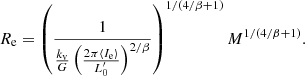
Although Eq. (1) is formally correct, it is incomplete and imprecise because it does not explicitly separate the mass of the stars and gas (baryonic mass in general) and the mass of dark matter, it does not specify the mass–radius relationship, and it also neglects the possibility that other terms due to other effects are present. To improve upon this issue, we can derive another expression for the theoretical log(L)−log(σ) relation based on the virial theorem developed by Caimmi (2003, 2009) in which dark matter (DM) and baryonic matter (BM) are treated separately. The details are given in Appendix A. This new log(L)−log(σ) includes (i) a suitable relation between the star mass (M*) and the total mass M = MDM + MBM; (ii) a suitable relation between the stellar mass M* and the effective radius Rs; and (iii) the redshift at which the collapse of the proto-galaxy has taken place. In other words we take the age of the bulk stellar population of a galaxy into account (see Fan et al. 2010). The relation is
 (3)
(3)
where Γ is the mean mass-to-light ratio of the galaxy, Kσ a term that includes the amount of DM, x the ratio between the DM and BM, y the ratio between the radius of the DM and BM matter components, and zf the redshift at the epoch of galaxy formation.
This way of writing the FJ relation in Eq. (3) indicates, at variance with Eq. (2), that both the exponent of the log(L)−log(σ) relation and its proportionality factor depend on the amount of DM in the galaxies (see Appendix A for all details) and are possibly variable factors.
In D’Onofrio et al. (2017) the authors proposed an alternative formulation of the FJ relation that can be used to explain the origin of the tilt of the FP and consequently the observed SRs. Their FJ-like relation, at variance with the classical FJ relation, holds for individual galaxies and not for a galaxy sample. In this formulation both the zero point and the slope vary from galaxy to galaxy and depend on the history of mass accretion and stellar evolution. To distinguish it from the FJ relation in Eq. (2), we write the new relation in the general form
 (4)
(4)
where L is in solar luminosities,  is a proportionality factor that strongly depends on the star formation history of each galaxy, and the exponent β reflects the peculiar motion of each object in the log(L)−log(σ) plane across the cosmic epochs. With numerical simulations we demonstrate in Sect. 5 that both β and
  are subject to variation from object to object and across the cosmic epochs. In particular the slope β turns out to have a spectrum of values ranging from large negative to large positive.
The new FJ-like relation hides the complex relationship existing between the baryon and DM components and the history of mass accretion and stellar evolution experienced by each stellar system. This relation is independent of the virial theorem. We guess that it is an equation that expresses the total luminosity of a galaxy independently of the total mass. Its existence is linked to the fact that luminosity, velocity dispersion, and star formation rate are mutually correlated in log units forming a plane as it occurs for the FP.
In the sections below using simulations we prove that the behavior of galaxies and GCs in the log(L)−log(σ), log(⟨I⟩e)−log(Re) and log(Re)−log(M*) planes are mutually connected, and that the observed distributions that we call SRs originate from the intersection of the virial theorem and the new FJ-like relation written for each single object. In particular, the values of β reproduce the main trends observed in the SRs.
4. Scaling relations of early-type galaxies and clusters
The above introduction was aimed at clarifying the framework in which we move if we want to understand the behavior of the SRs. In this section we start to discuss the observed distribution of galaxies and clusters in the main SRs, highlighting in particular the comparison between ETGs and clusters.
4.1. The log (L) − log(σ) plane
The distribution of our systems in the log(L)−log(σ) plane is presented in the left panel of Fig. 1. The data sample includes in this case the faint ETGs studied by Bettoni et al. (2016), the normal ETGs studied by D’Onofrio et al. (2017), the II-BCGs and BCGs from Paper I, and the GCs studied by Cariddi et al. (2018). The figure clearly shows that there is a well-defined linear trend in log scale between total luminosity and velocity dispersion for all systems, from faint ETGs to big clusters. The solid black line in the figure marks the least-squares orthogonal fit obtained by the program SLOPES (Feigelson & Babu 1992) for the whole set of data. The coefficients derived with the different types of SLOPES analysis are listed in Table 1. The correlation coefficient is c.c. = 0.82 and the rms scatter is 0.32. The three boxes of the table refer to the whole dataset of real galaxies (upper box), the subsample of normal ETGs (middle box), and the whole sample of simulated objects (lower box). The table also give the errors on the parameters obtained with all the bootstrap and jackknife analyses by SLOPES.
 |
Fig. 1. Left panel: distribution of ETGs and clusters in the log(L)−log(σ) plane. Black filled circles indicate our BCGs, red filled circles our II-BCGs, small gray filled circles the 1729 normal ETGs used by D’Onofrio et al. (2017) to study the FP, gray empty stars the faint ETGs of Bettoni et al. (2016), and blue filled circles our clusters. The normal ETGs reanalyzed in Paper I are not shown because their sigma values are not available. The black solid line gives the best fit of the whole dataset obtained with the orthogonal method. The dotted line shows the L ∝ σ2 law predicted for virial systems, while the dashed line gives the L ∝ σ4 FJ slope. Error bars are not shown because they are approximately as big as the plotted filled circles. Right panel: log(L)−log(σ) plane for real and simulated objects. The color-coding and symbols are the same as before. The open circles are used for simulated objects using the same color-coding. The plotted lines are the same as in the left panel. |
Coefficients of the log(L)−log(σ) relation with the different methods provided by the SLOPES program.
The slope is close to the value of 4 originally proposed by Faber & Jackson (1976) (shown by the dashed line). We note that the log relation is quite linear and seems valid almost independently of the mass and size of the systems, and has approximately the same zero point for all objects (within the observed scatter of 0.32). We also note that the exponent is ∼3, quite close to that predicted in Sect. 3 above, but different from 2, the value expected for virialized systems.
We observe that the orthogonal fits are approximately consistent with a slope of ∼3 for the whole set of systems and for real galaxies. A lower value is observed for simulated galaxies. In general we note that the slopes are different when different methods are used to derive the fits. This is due to the different sizes of the samples. We have approximately 2000 ETGs, 60 GCs, and 25 DGs. Clearly the result of the fit is strongly affected by the distribution of ETGs. The coefficients of the fits obtained for the single subsamples might also largely deviate from each other, in particular for the DGs and GCs that have a clumpy distribution.
The right panel of Fig. 1 shows the data of the Illustris simulation for the brightest galaxies (BCGs and II-BCGs) and the faint ETGs. We can say that a qualitative good agreement with observations exists. The agreement is poorer for GCs and faint ETGs, the former appearing systematically fainter in luminosity and with a smaller central velocity dispersion, while the latter being a bit brighter with respect to the observed trend of faint ETGs. The difficulty of simulations in reproducing the properties of clusters and faint ETGs were already noted in Paper I. Most of the simulated objects are approximately distributed along the slope of 2 predicted for virialized objects (the dotted line). This is due to the fact that the velocity dispersion of clusters have been obtained from the virial relation, while the measured ones were calculated on the basis of the redshift differences of the galaxies with respect to that of the central BCG. Unfortunately, the data of the simulation does not permit an easy way to derive the GC velocity dispersions.
At this point it should be noted that our aim is not that of determining the best slope of the FJ relation, nor to quantify the agreement between real and simulated data; we are simply comparing qualitatively the distributions of real and simulated galaxies. We believe that the observed position of all these systems, both real and simulated, in this plane is sufficient to agree on the fact that they all follow a quite similar trend, whatever the correct slope is.
The existence of the log(L)−log(σ) relation has never been interpreted as a physical link between galaxy luminosity and velocity dispersion. The common explanation for the tilted slope with respect to the virial expectation is that there is a smooth variation in the stellar population (variation in M/L) and/or a smooth variation in non-homology (variation in kv and n) (see D’Onofrio et al. 2017) across the whole systems. The reason for the mismatch is the same as for the FP. In the log(L)−log(σ) relation L is used instead of the combination of Re and ⟨μ⟩e. The tilt occurs because Eq. (2) is valid for only one galaxy and not for the whole set of ETGs. Each galaxy is in virial equilibrium, but the zero point is different for each system. If this interpretation is correct, the question is how the variations in structure and stellar population occurring in the galaxies through the cosmic epochs can preserve the small scatter being L0 and β variable factors. This is the well-known fine-tuning problem already encountered in the FP (D’Onofrio et al. 2017). The existence of a fine-tuning mechanism between galaxy structure and stellar population is difficult to reconcile with the idea of galaxies continuously merging and interacting among each other, as shown by the modern numerical simulations.
In Sect. 5 we demonstrate through simulations that the current slope of this relation originate from the global complex mass assembly history of galaxies, that clearly affect either the mass-to-light ratio and the structure of the systems.
4.2. The log(⟨ I ⟩e)−log(Re) plane
Kormendy (1977) first recognized that the distribution of ETGs in the log(⟨I⟩e)−log(Re) plane is not random and that the slope of the observed distribution is not that predicted for simple virialized systems.
Remembering Eq. (2) and using the definition of surface brightness we can write
 (5)
(5)
so that in log units the slope of the virial log(⟨I⟩e)−log(Re) relation is −1. For systems along this line (i.e., with the same zero point and similar kv) the mass-to-light ratio M/L should scale with σ according to M/L ∝ σ2.
The left panel of Fig. 2 shows how our galaxies and clusters are distributed in this plane. The distributions of BCGs, II-BCGs, normal ETGs, faint ETGs, and clusters do not follow the slope predicted by the virial theorem, but a much steep trend (look at the solid line between the dotted line predicted for systems of equal luminosity with slope −2 and the dashed line). This is the line found by Capaccioli et al. (1992) that best fits a much larger sample of bright ETGs. The slope is −1.2 (which in surface brightness units is 3; ⟨μ⟩e = 3.0log(Re kpc)). In their work Capaccioli et al. (1992) distinguished two different families of ETGs in this plane: the ordinary family with faint luminosity and small radii, and the bright family with high luminosity and large radii. These two families are distributed in a completely different way in the log(⟨I⟩e)−log(Re) plane, probably for the different role of merging in their formation. The ordinary family is clearly visible with the present sample in Fig. 2: it is made up of objects with Re ≤ 4 kpc (the green dots, the open magenta stars, and the green filled circles). D’Onofrio et al. (2014) already showed that spiral galaxies are confined to the ordinary family (their Fig. 9). The figure clearly indicates that only the brightest ETGs develop the tail well known as the Kormendy relation. The ZoE in the figure is the region empty of points above the dashed line with slope −1 for virial systems. We show in Sect. 4.4 how the zero point of this line has been obtained.
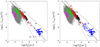 |
Fig. 2. Left panel: distribution of galaxies and clusters in the log(⟨I⟩e)−log(Re) plane. Black filled circles indicate our BCGs, red filled circles our II-BCGs, green filled circles our random sample of normal ETGs, gray filled dots the 34982 galaxies analyzed by D’Onofrio et al. (2014) with GASPHOT, empty magenta stars the faint ETGs of Bettoni et al. (2016), and filled blue circles our clusters. The dashed line with slope −1 is that predicted for virialized systems for a possible ZoE. The zero point of this line was chosen as explained in Sect. 4.4. The dotted line is that expected for systems of equal luminosity MV = −21.5 with slope −2. The solid line with slope −1.2 is that obtained by Capaccioli et al. (1992). Right panel: log(⟨I⟩e)−log(Re) plane with real and simulated objects. The color-coding and symbols are the same as before. The open circles with the same colors of real galaxies are used for simulated objects. The plotted lines are the same as in left panel. |
In Fig. 2 we see that clusters share the same properties of big ETGs. Their position is at low surface brightness and large radii along the line fitting the high luminous galaxies. Clusters therefore follow the same log(⟨I⟩e)−log(Re) relation of bright ETGs.
In Paper I, when we compared the light profiles of clusters and ETGs, we concluded that clusters are more similar to faint ETGs than to BCGs. Here instead we see the opposite. When we consider the structural parameters they are more similar to BCGs. We provide a possible explanation of this behavior in Sect. 6.
The right panel of Fig. 2 shows the log(⟨I⟩e)−log(Re) plane with simulated data. For each simulated object at z = 0 we derived the growth curve luminosity profile and the main structural parameters (e.g., Re, ⟨I⟩e, σ) following the same procedure used for real galaxies. We can therefore compare the position of the simulated structural parameters (open circles) with the real ones. The good agreement achieved by simulations for BCGs, II-BCGs, and normal ETGs, and the failure for clusters is evident. Clusters are systematically smaller in size and brighter in surface brightness. This confirms what we claimed in Paper I.
The left panel of Fig. 3 shows an enlargement of the log(⟨I⟩e)−log(Re) plane in the area covered by galaxies. We note how the simulated data for the whole set at z = 0 shown by the small red dots are able to reproduce both the ordinary and bright family defined by Capaccioli et al. (1992, their Fig. 4). The simulations fail only in the zero point of the surface brightness that appears systematically brighter than that of real galaxies. This effect is not visible in the right panel of Fig. 2; in that case the effective radius and the effective surface brightness were obtained from our careful analysis of the light profiles of BCGs and II-BGCs done in Paper I, while here we used the half-mass radius of the Illustris dataset that might be a bit different from the effective radius. The simulations also seem to fail in the effective radius of the faint ETGs that appear systematically bigger with respect to that of real objects.
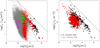 |
Fig. 3. Left panel: enlargement of the log(⟨I⟩e)−log(Re) plane with real and simulated galaxies. Black filled circles indicate our BCGs, red filled circles our II-BCGs, green filled symbols our random sample of normal ETGs, gray filled dots the WINGS ETGs of D’Onofrio et al. (2017), empty stars the faint ETGs of Bettoni et al. (2016), and filled circles our clusters. The small red dots are used for the whole set of Illustris galaxies at z = 0. In this case the effective mass radius is assumed to be equal to the effective radius. The dotted line is that expected for systems of luminosity MV = −21.5. Right panel: log(⟨I⟩e)−log(Re) plane for cluster (black dots) and non-cluster (red dots) ETGs. Shown is the subsample of galaxies with available masses from Fritz et al. (2007). In both panels the dashed lines are the trends for virialized systems with slope −1 and a zero point of a possible ZoE. |
The right panel of Fig. 3 shows the log(⟨I⟩e)−log(Re) plane for cluster and non-cluster ETGs. In this case we used the subsample of the WINGS galaxies with available masses derived by Fritz et al. (2007). We note how the tail of galaxies with large Re is present only for cluster objects, while is almost absent for field objects.
Capaccioli et al. (1992) attributed the origin of the bright family to mergers. The data therefore seem to suggest that in the cluster environment galaxies experience more merging events. The large number of minor dry merging events and the stripping phenomena could in fact inflate the radius of ETGs, in particular in the central region of the clusters (see, e.g., Naab et al. 2009).
D’Onofrio et al. (2017) showed that by using Eq. (4) with negative values of β it is possible to fit the observed distribution of the bright ETGs in the log(⟨I⟩e)−log(Re) plane (i.e., to obtain the Kormendy relation; Kormendy 1977). This occurs because two intersecting planes can be defined for each object in the 3D log(⟨I⟩e)−log(Re)−log(σ) space: one representing the mass of the galaxy (through the virial equation) and one representing the luminosity (provided by the log(L)−log(σ) relation). The intersection between these planes generates a line in the log(⟨I⟩e)−log(Re)−log(σ) space that can be observed projected in the log(⟨I⟩e)−log(Re) plane. When β is negative it is possible to fit the distribution of the bright ETGs and clusters. The slope of this line in the log(⟨I⟩e)−log(Re) plane is given by Eq. (17) in D’Onofrio et al. (2017), that we rewrite here as
 (6)
(6)
where Π is a factor that depends on kv, M/L, β, and L0. Table 2 gives for each possible value of β the corresponding slopes in the log(⟨I⟩e)−log(Re) (and ⟨μ⟩e − log(Re)) relation. These slopes represent the direction of motion of a galaxy in this space along a cosmic time interval. We note how progressively large negative values of β, which are peculiar to galaxies in a quenched state, determine values of the slope in the log(⟨I⟩e)−log(Re) plane converging toward the expected virial value of −1. The luminosities of these galaxies progressively decreases at nearly constant velocity dispersion, a behavior of objects in passive stellar evolution.
Different values of β and the corresponding slopes in the log(⟨I⟩e)−log(Re) and ⟨μ⟩e − log(Re) planes.
This means that the ZoE is not only the locus of undisturbed virialized galaxies, but also that of purely passive evolving systems. Notably, this slope does not depend on the mass of the system and is the same for all types of objects, from stars to galaxy clusters. The zero point of the ZoE, on the other hand, depends on the mass-to-light ratio and the non-homology reached by systems when they arrive at the condition of passive evolution and virialization. As galaxies get older their M/L values tend to increase asymptotically providing a maximum possible value for all stellar systems. In the V band the maximum measured stellar mass-to-light ratio is ∼20. Young objects cannot cross this boundary limit. This might suggest that the undisturbed virialization of galaxies can be reached only when systems enter the passive evolution. In this condition, when no more energy is injected in the galaxy from star formation, AGN, and SN feedbacks, the system can relax and enter progressively in the trend predicted by the virial theorem. Its final position in those planes will clearly depend on the zero point reached when these conditions are met.
4.3. The log(Re)−log(M*) plane
When a galaxy is in the virial equilibrium one might expect that the stellar mass scales linearly (with slope 1 in log units) with the effective radius as in Eq. (1).
In Fig. 4 we observe the distribution of normal galaxies, BCGs, and GCs in the log(Re)−log(M*) plane. We see that clusters (blue dots) follow the same distribution of BCGs (green dots) and ETGs of mass greater than 1010 M⊙ (black dots). We recall that we used only the clusters that are well fitted by the r1/n law, i.e., those much closer to a virial equilibrium not disturbed by secondary components likely due to recent merging events. The red small dots are the data coming from Illustris. The solid line that best fits this distribution of galaxies and clusters has a slope of ∼0.9, very close to the value of 1 coming from the virial theorem (shown by the dashed line) that here also represents the ZoE of the log(Re)−log(M*) plane. To the right of this line there are no objects. The zero point of this relation is discussed in Sect. 4.4. The same figure shows the distribution obtained for the simulated galaxies as red dots. We note that the simulation catches the high mass tail, while it fails for the low masses.
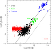 |
Fig. 4. Distributions in the log(Re)−log(M*) plane for normal ETGs (black filled circles), BCGs (green filled circles), and clusters of galaxies (blue filled circles) from our WINGS samples. The red small dots show the data of the Illustris simulations for galaxies at z = 0. The solid line is the fit of the galaxies and cluster sample, while the dashed line is the slope predicted from the virial theorem for a possible ZoE. |
Figure 5 shows the stellar mass–radius relation derived only for the WINGS galaxies. Here we used the whole set of WINGS galaxies with available stellar masses mentioned in the Introduction that was calculated using the K luminosity as a proxy. We only distinguish the various galaxies on the basis of membership and morphology (ETGs and LTGs). Cluster member objects are plotted in the upper panel and non-member galaxies in the bottom panel. ETGs are shown as open circles, while LTGs as filled circles. The membership was evaluated by Cava et al. (2009) on the basis of the redshift and the morphology by Fasano et al. (2012). We note that the tail in the log(Re)−log(M*) plane is primarily due to massive ETGs and is almost absent for spirals and for field objects. Is this behavior due to a selection bias? The distribution in redshift of the field sample peaks at ∼0.1, while that of clusters at ∼0.05. This is a potential source of bias for the present comparison, but simulations have revealed that Re does not change significantly in this redshift interval. The interval of mass is also quite similar, so that we can be quite confident that the observed difference is not originated by selection effects. In addition we know that the galaxies with the largest radii are also the most luminous, so that we can exclude a Malmquist bias.
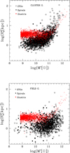 |
Fig. 5. Stellar mass–radius relation for galaxies in clusters (upper panel) and in the field (bottom panel). The open black circles show the real ETGs, the black filled circles the spiral galaxies, and the red dots the simulated data at z = 0. The stellar masses used here were derived from the K-band luminosity of our galaxies. |
In the two panels the data of the Illustris dataset at z = 0, derived only for the galaxies in clusters, are again shown as small red dots. The banana-like shape of the distribution of real galaxies is not well reproduced. In the Illustris-TNG the effective radii are a bit lower than in Illustris-1, but it is seems that they are on average still highier by a factor of 3 with respect to observed data (see Fig. 1 of Genel et al. 2018).
We verified that the galaxies in the tail are the same as observed in the tail of bright galaxies in Fig. 2. The tail is formed primarily by massive quenched objects at the center of clusters that have likely increased their radius because of the frequent dry merger events. To the right of this tail there are no galaxies. This is the ZoE region of the log(Re)−log(M*) plane. We show below that the slope followed by massive quenched passive objects in this diagram is the same as that predicted for virialized systems.
Figure 6 shows the distribution of ETGs and LTGs in clusters and in the field using different colors for the different ranges of the B − V index of galaxies. The red objects are preferentially distributed in the right part of the diagram (i.e., closer to the ZoE). Furthermore, the banana shape is more evident for ETGs than for LTGs. The trend is almost absent for LTGs in the field, while for objects in clusters the relation is always present. The LTGs in clusters seem to share a log(Re)−log(M*) relation not present in the field. Again, we are led to think that even LTGs grow in size in the cluster environment. A very similar trend is seen when different ranges of the Sérsic index n are considered. This means that the structure of the galaxies also changes along the sequence: high values of the Sérsic index are measured only for the galaxies in the tail, while low values of n are typical for the flat part of the sequence.
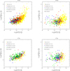 |
Fig. 6. log(Re)−log(M*) relation for ETGs and LTGs in clusters (left panels) and in the field (right panels). Galaxies are plotted in different colors according to their B − V color index. |
Table 3 shows the coefficients (slope and intercept) of the best-fit linear relation for the galaxy distribution in the log(Re)−log(M*) plane, when different ranges of masses are selected. The best-fit relation was obtained with the standard least-squares fitting technique (using the program SLOPES of Feigelson & Babu 1992). It is clearly visible that the slope increases when massive galaxies are taken into account: we start from 0.13 (when low mass systems are fitted) and we end up with 0.68 (when only the most massive systems are fitted). The slopes of the fit changes slightly if the bilinear least-squares fit is applied, reaching values up to 1, when the fit is done only for the massive galaxies (log(M* > 10.5)). The average errors on the slopes and intercepts are on the order of 0.02 and 0.2, respectively. This means that the observed differences are significant.
Slope and intercept of the best-fit log(Re)−log(M*) relation for different mass ranges.
This behavior demonstrates that the distribution of galaxies in the diagram is curved. The origin of the trend should be searched in the different conditions of virialization and density distribution inside the single galaxies. The pure virial behavior of Eq. (1) with a similar zero point seems to be valid only for the most massive and red systems. In less massive ETGs and in LTGs rotation is progressively more important, as is the DM content. It is also possible that dwarf systems are not in a full virial equilibrium yet, being still affected by episodes of star formation and in general suffering the interactions with the cluster environment (stripping and harassment). They might not be fully relaxed from an energetic point of view, presenting a radius much larger than that expected for a virial system of that mass. These two effects could be at the origin of the curved distribution of the log(Re)−log(M*) relation. We analyze this relation in more detail in Paper III of this series (Chiosi et al. 2020). We only want to note that the observed distribution reveals a systematic change in zero point of the virialized galaxies. This variation has also been invoked to explain the tilt of the FP and FJ relation, and the observed distribution in the log(⟨I⟩e)−log(Re) plane tilted with respect to the virial prediction.
We now show what happens when we combine Eq. (1) with Eq. (4). A simple algebra gives
 (7)
(7)
In Table 2 we list the values of the predicted slopes for the log(Re)−log(M*) relation on the basis of the possible values of β (i.e., once the virial plane and the FJ-like relation are combined). It should be noted that the slope of the log(Re)−log(M*) relation is in agreement with the values fitted on the observed distribution provided in Table 3 below. The resulting curved distribution is clearly obtained by the progressive change of the slope and the zero point, both depending on β. The zero point turns out to depend on kv,  , and ⟨I⟩e. This explains why the log(Re)−log(M*) relation presents different distributions according to the values of the Sérsic index, the age of the galaxies (Valentinuzzi et al. 2010), and mean surface brightness (see, e.g., Sanchez Almeida 2020). The massive passive galaxies with large negative values of β converge toward values of the slope close to 1 (the value predicted for virialized systems). On the other hand, the lower slope observed for spiral galaxies is also in good agreement with values of β close to ∼3.
In conclusion we see that the combination of the virial theorem and the FJ-like relation can explain the observed trends in the log(⟨I⟩e)−log(Re) and log(Re)−log(M*) relation, and also the FP (D’Onofrio et al. 2017).
4.4. Zone of exclusion
We have suggested that the slopes of the ZoE in the log(Re)−log(M*) and log(⟨I⟩e)−log(Re) planes could have the values predicted by the virial theorem for fully relaxed systems. The slope is −1 in the log(⟨I⟩e)−log(Re) plane and 1 in the log(Re)−log(M*) plane. In these figures we have always drawn the possible ZoE with dashed lines. The problem now is, what is the zero point of the ZoE? This can be derived from Eqs. (1) and (5) once the values of kv, M/L, and σ are known. Unfortunately, the total mass M of our systems is unknown, but we can have an idea using M*. The value of kv for every system can be approximately obtained from the Sérsic index n using Eq. (11) of Bertin et al. (2002) (considering only the structural non-homology). The stellar masses of galaxies are known from the SED fitting of the spectra and from the stellar mass-to-light ratios of clusters measured by Cariddi et al. (2018). The stellar velocity dispersion is also available for many objects from the WINGS database. Figure 7 shows the different zero points calculated for our systems in the log(Re)−log(M*) and log(⟨I⟩e)−log(Re) planes. We have added here a sample of globular clusters (magenta points). These systems are likely in a good virial equilibrium state and can therefore be used as reference comparison objects. The data are those of Pasquato & Bertin (2008). For globular clusters we assumed the perfect homology with a Sérsic index n = 4.
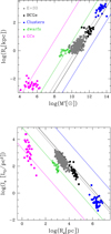 |
Fig. 7. Upper panel: log(Re)−log(M*) plane. GCs are shown as magenta dots, dwarfs as green stars, normal ETGs as gray dots, BCGs as black dots, and clusters as blue dots. Each colored line indicates the average zero point of the systems calculated from Eqs. (1) and (5) with the values of kv, M*/L, and σ. The solid black line is obtained for the sample of galaxies and clusters taken together. All the lines have the slope 1 predicted for virialized systems. Lower panel: log(⟨I⟩e)−log(Re) plane. The same color-coding is adopted. Here the slope of the lines is −1. |
Figure 7 shows in the upper panel the log(Re)−log(M*) plane with the objects in our sample: globular clusters, normal ETGs, faint ETGs, BCGs, and galaxy clusters. The virial relations are shown (with slope 1) with the different zero points calculated for each system: ZPMR = G/(kvσ2). We take as ZPMR the average value of all zero points for each sample of objects considered. We note that the predicted linear trends with these calculated zero points intercept the distribution of each sample. The lines however do not cross the distribution exactly in the middle. This is due to the fact that the variable sigma depends on the total mass of the system, while here we consider the virial relation using the stellar mass. We show below that by using Eq. (1) we can get the velocity dispersion σ* that a galaxy would have if DM were absent.
In the bottom panel we can see the log(⟨I⟩e)−log(Re) plane where we have calculated the zero points of our systems through the formula: ZPIeRe = (kvLσ2)/(2πGM*). The colored dots show the same sample of objects. Again, we note that the location of the zero points provide virial lines intercepting each system, but not in the middle of the observed distribution.
It should also be noted that the zero points of systems more massive than 1010 M⊙ are approximately similar and seem to converge toward the limit of the ZoE. We checked that the combination of the variables kv, σ, and M*/L is such that very similar values are obtained in log scale for all these systems.
In Fig. 8 we show the difference between the measured σ and those calculated from the virial equation, before (upper panel) and after (bottom panel) a correction applied to the stellar mass M*. In order to have a mean difference equal to zero we need to correct the stellar masses of the following quantities: a factor of 1.66 for dwarfs, 1.25 for normal ETGs, an ∼40 for GCs. These objects appear dominated by the DM. We do not consider globular clusters because they are not affected by DM and they can lose mass during their crossing of the Milky Way disk.
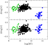 |
Fig. 8. Stellar mass vs. difference in log units of the velocity dispersion measured from spectra and calculated through the virial equation. Upper panel: difference before the correction of the stellar mass. Lower panel: indicates that once the mass is corrected for the contribution of DM the two quantities are in good agreement (see text). Black dots are normal ETGs, green dots the faint ETGs measured by Bettoni et al. (2016), blue dots are galaxy clusters. |
In conclusion of this section we can say that all our objects are in virial equilibrium. However, as we see in the next section, the simulations suggest that the virial equilibrium might be continuously disturbed by merging, stripping, and interaction events. While in massive galaxies the impact of merging, stripping, and interactions with objects of smaller mass can be of minor relevance, in dwarf galaxies these events may induce severe disturbances. The inner total energy of dwarf galaxies can vary significantly when even minor mergers occur. In this sense we can speak of a condition of “undisturbed virialization” for a galaxy when no more merging–stripping and star formation events are in place or when the galaxy is so massive that is no more affected by the small merging or stripping events.
If our view is correct, the ZoE is the natural border of undisturbed virialized systems that have reached the maximum possible values for σ, kv, and M/L. We do not know its exact position because the DM contribution is unknown, so we have chosen an arbitrary value in Figs. 2 and 5.
By means of simulations we show that the condition of undisturbed virialization is reached only by massive ETGs. They are passive and quenched objects. They are so massive that new encounters or mergers do not significantly alter their virial equilibrium.
5. Evolution of the scaling relations with redshift
In this section, with the aid of the Illustris library of galaxy models, we examine the cosmic evolution of the above mentioned SRs. We use the whole dataset of simulated objects with mass larger than 109 M⊙ at z = 0 present in the selected clusters. Each galaxy is followed along its evolutionary tree (in this case along the main progenitor branch, i.e., that following the mass history), since z = 4, a history made of merging events, tidal interactions, periods of quiescence, as well as BH and SNe activities3.
Prior to any other consideration, by means of SSPs of different ages and metallicities we examine the luminosity evolution of a galaxy, either in isolation or in the presence of bursts of star formation that are triggered by mergers with galaxies of comparable mass. Masses are set equal to those of typical galaxies in the mass interval 107 to 1012 M⊙. We call this type of galaxy model SSP galaxies. Starting from this, we set up Monte Carlo simulations of bursts of star formation in already existing seed objects of given mass, age, and metallicity (varying the burst age and intensity) and/or simulations of mergers among galaxies of different mass, age, and metallicity (varying the time of fusion). The details of the Monte Carlo method are shortly given in Appendix B.
In Fig. 9 we show the luminosity evolution of a 109 M⊙ SSP galaxy undergoing bursts of star formation of different age and intensity (expressed by the percentage of mass going into stars). In our simulations this percentage is assumed to be 30% of the galaxy mass. The age of the galaxy is fixed to 13 Gyr and its mean metallicity is estimated from the mass–metallicity relation in Table B.1, which is from Sciarratta et al. (2019). The ages of the bursts are 7 Gyr (oldest), 2 Gyr, and 1 Gyr (youngest). As expected, the luminosity evolution expressed by the absolute visual magnitude Mv depends on the burst age. The oldest one is in practice indistinguishable from the case of the unperturbed galaxy (thick black line), whereas for the youngest one we expect a present day absolute magnitude about 1 mag brighter than for the unperturbed case.
 |
Fig. 9. Results of dissection of single bursts inside 13 Gyr SSP galaxies: evolution with time of Mv for the SSP galaxy with log M = 9 (Z = 0.004) perturbed by a single burst with mass fraction of 30%; solid thin curves are, in terms of increasing age, magenta (1 Gyr), blue (2 Gyr), and orange (7 Gyr); the thick black line is the unperturbed case shown for comparison. |
Similar results are obviously possible when varying the galaxy mass. This is achieved by simply scaling up and down by the luminosity of the 109 M⊙ objects by the quantity 10−0.4ΔM.
Mergers among galaxies of different mass and age would yield similar results, the variation in absolute magnitude (luminosity) being driven by the variation in mass and age of the two component galaxies, together with a small contribution due to different mean metallicity of the galaxies. If mergers are also accompanied by a revival of the star formation activity an additional variation in the present day luminosity is expected. Finally, if a galaxy of a certain age and mass suddenly stopped star formation, its luminosity would soon fall onto the luminosity–age relation of the passive case (the timescale involved would be on the order of 1 Gyr or less).
The main conclusion is that the luminosity (in the V pass-band in this case) significantly depends on the particular star formation history of each galaxy, in such a way that it cannot be easily traced back from the present-day properties. This example clearly shows that a significant dispersion in the V-luminosity of a galaxy of given mass is possible and also expected. This would blur the proportionality factors L0 and/or  of Eqs. (2) and/or (3). The expected blurring in luminosity is Δlog(L)≃0.4, i.e., very close to the observed dispersion in the log(L)−log(σ) relation.
Figure 10 shows the log(L)−log(σ) relation expected from the Illustris simulation at different cosmic epochs: galaxies at z = 4, at z = 1, and at z = 0. It is worth recalling that the objects at z = 4 are the progenitors of those at z = 1, which in turn are the progenitors of those at z = 0. We clearly see that going toward the present epoch the global distribution of galaxies is progressively less steep, but the scatter is very similar. The slope/rms decreases from 5.49/0.24 at z = 4 to 3.54/0.17 at z = 1 and to 2.71/0.18 at z = 0. We note that the log(L)−log(σ) relation is rather narrow at any redshift. A little change in slope also seems be present for the brightest galaxies after z ∼ 1, with a smooth flattening of the relation toward lower slopes.
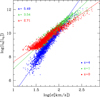 |
Fig. 10. Simulations of the log(L)−log(σ) relation with the galaxies of the Illustris dataset at three different redshifts. Objects at z = 0 are shown as red dots, at z = 1 as green dots, and at z = 4 as blue dots. The colored lines show the best fits of the distributions and the resulting slopes are listed in the top left corner. |
Globally the relation seems to rotate with time around a point approximately located at σ = 100 km s−1 and L = 1010L⊙. This means that on average the points move in a direction almost perpendicular to the observed relation reinforcing the idea presented in Sect. 3 that the log(L)−log(σ) relation should be written in the form of Eq. (4), where both  and β are variables. In this way galaxies can move in this plane along paths that depend on the peculiar merging–interaction events and on the SFH.
Finally, there is another important remark to be made, looking at the log(L)−log(σ) relation at different redshifts. In Fig. 10 we note that at a given redshift the dispersion Δlog LV decreases at increasing sigma (mass) of the galaxy. The explanation relays on the merger mechanism itself: by increasing the mass of a galaxy the probability of merging another object of comparable mass (so that the effect on the luminosity would be sizable) decreases in compliance to the number density when varying the galaxy mass, the so-called funneling effect amply discussed by Sciarratta et al. (2019, references therein). As a result, as the redshift tends to zero, high mass objects engulf galaxies of small mass so that the net effect on their luminosity becomes very small.
The evolution of the log(L)−log(σ) relation is in line with the moderate evolution of the FP coefficients found by Lu et al. (2019) from z = 0 to z = 2 with the data of the IllustrisTNG simulation (Alberini et al., work in progress).
From the values shown earlier of β, that each galaxy can have during evolution, we might understand the global behavior of the SRs. The galaxies move in the log(⟨I⟩e)−log(Re) and log(Re)−log(M*) plane in a direction fixed by the values of β. Here we try to estimate the values of this parameter using the results of simulations. The starting point is to recognize that β is given by the slope of the line connecting two different location of the same galaxy in this plane.
In Fig. 11 we see the paths of few single galaxies in the log(L)−log(σ) plane from z = 4 to the present. They are complex and clearly mirror the effects of several variables. Each path is made of many steps in which the mass and velocity dispersion are varied. In general there are long steps in which the mass is significantly increased–decreased by mergers–interactions, and short steps in which the mass and velocity dispersion vary by small amounts. The steps may have different inclinations in the log(L)−log(σ) plane. The evolution starts at z = 4 (blue dots) and goes through z = 1 (green dots), ending at z = 0 (red dots). The black lines follow each path along the various redshift epochs.
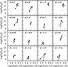 |
Fig. 11. Path of single galaxies in the log(L)−log(σ) plane from z = 4 (blue dot) to z = 0 (red dot). Within each box is the value of the slope β of the trajectory connecting the two epochs. |
Empirically we can define a mean path (e.g., from z = 4 to z = 0) considering the line connecting the two points (blue and red) in this diagram, and an instant path connecting the two points at redshift z = 0.2 and z = 0 (the two closer epochs). The exact value of β today is unknown. We can only estimate its values during past intervals of time that have seen a galaxy to change its luminosity and velocity dispersion.
At the top left of each panel in Fig. 11 we list the value of β, the exponent that enters in the log(L)−log(σ) relation that can be obtained measuring the slope of the line connecting the points at z = 4 and z = 0. We note the high spread of values of β, spanning both negative and positive values. Positive slopes up to about 5 are expected in the presence of mergers among galaxies of comparable mass. Higher positive values deserve some care and attention because mergers among galaxies of similar mass are becoming less important and other secondary effects on the log(L)−log(σ) relation could show up. Very high negative slopes (e.g., below −5) are also of interest because they indicate the presence of important episodes of mass removal (thus masking the effect of the initial redshift on the velocity dispersion). Particularly interesting are the cases with negative slopes in the bin 0 to −5, which are very frequent (this is the second most populated bin of the distribution in the domain of negative slopes) and the mean slope of the whole sample with redshift from z = 4 to z = 0, which is close to −1. Finally, very negative β are those belonging to passive systems, quenched objects where the luminosity is progressively decreasing.
We evaluated the mean slope of the paths for two different groups in redshift: from z = 4 to z = 0 (galaxies followed up to the far past, i.e., ∼12.1 Gyr ago) and from z = 0.2 to z = 0 (galaxies followed up to the recent past, i.e., ∼2.4 Gyr ago). The resulting slopes for the two intervals in cosmic epochs are shown in the left panel of Fig. 12. The two distributions of β peak in the interval 0 to ≃3 ÷ 4 and nearly symmetrically extend to very high negative and positive slopes. The average slope is −1 for the case in which galaxies are followed from z = 4 to z = 0, while it is ∼3 for the case containing galaxies traced back from z = 0.2 to z = 0. On the other hand the medians both peak around ∼3. The red histogram shows the values of β measured for the lines connecting the dot at z = 4 with the dot at z = 0. The black histogram instead gives the distribution of β for the more recent epoch (from z = 0.2 to z = 0). The median values of the two distributions are reported in the plot. Notably, the median values peak approximately at the slope observed for the real log(L)−log(σ) relation. This means that the fit of the observed distribution is primarily influenced by the complex history of mass assembly of the single galaxies. We note that the most common path corresponds to the slope of the observed FJ relation.
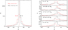 |
Fig. 12. Left panel: distribution of the slope β for the whole sample of galaxies. The red histogram shows the values of β measured from z = 4 to z = 1, the black histogram from z = 0.2 to z = 0. The dashed lines give the medians of the distributions. Right panel: distribution of the slope β for the galaxies of different masses. The red histogram shows the values of β measured from z = 4 to z = 0, the black histogram from z = 0.2 to z = 0. |
The right panel of Fig. 12 shows the same histograms for different bins of galaxy masses. The average slope varies considerably for the different mass ranges (see Table 4), while the median is always positive. This implies that galaxies of different masses experience different events with different consequences.
Average and median values of β for the two intervals in cosmic epochs in the different mass ranges.
If we differentiate Eqs. (A.14) and (A.15) we can get an idea of the main contributions in ΔL and Δσ that determine the shifts of the points in the log(L)−log(σ) plane. The mass term dominates, while the other terms do not contribute in a significant way.
Figure 13 shows the paths of four galaxies in the log(⟨I⟩e)−log(Re) plane. In the figure we show in blue the galaxy distribution at z = 4, in green that at z = 1, and in red that at z = 0. In the upper panels the black lines show the evolution of two galaxies that at z = 0 are observed in the tail of the log(⟨I⟩e)−log(Re) relation (i.e., objects belonging to the bright family), while in the bottom panels that of objects of the ordinary family. In general the paths are very different for each galaxy: the position in the diagram appears strongly influenced by the mass assembly history.
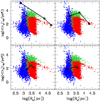 |
Fig. 13. Four different paths in the log(⟨I⟩e) −log(Re) plane resulting from simulated data. Blue dots give the distribution at z = 4, green at z = 1, and red at z = 0. The half-mass radius in parsecs is assumed to be equal to the effective radius. The black lines connect the same object at different epochs. |
It should be noted that large positive values of β produce positive slopes in the log(⟨I⟩e)−log(Re) plane that could not belong to objects of the bright family. These objects have already reached a passive evolution. Positive values of β can be observed only for galaxies of the ordinary family. On the other hand, large negative values of β converge toward a limiting slope in both the log(⟨I⟩e)−log(Re) and log(Re)−log(M*) relation (see Table 2).
The formation of the bright family tails in the log(⟨I⟩e)−log(Re) and log(Re)−log(M*) planes is very interesting. The simulations are able to reproduce such peculiar features, for example the observed distributions of bright galaxies in the log(⟨I⟩e)−log(Re) plane and the steeper part of the log(Re)−log(M*) relation. Both sequences are formed by objects with mass higher than 1010 M⊙. How do they originate? We see from the simulations that these tails are absent at earlier epochs (before z = 2). If the tails originate from the merging activity, what kind of merger is it? We speculate that dry mergers are responsible for these features. The merging of stars without gas might inflate the systems because the global energy is not dissipated by heating the gas. The absence of gas is also apparent from the fact that there are no associated star formations (the tails are made by the most red galaxies).
Figure 14 shows the paths of three galaxies in the log(L)−log(σ) (left panel), log(⟨I⟩e)−log(Re) (middle panel) and log(Re)−log(M*) (right panel) planes. Again, dots of different colors give the position at different redshifts. We note that the ETGs in the log(Re)−log(M*) plane have the highest mass and radius, in the log(L)−log(σ) plane they move toward a lower luminosity (i.e., have a negative slope β), and in the log(⟨I⟩e)−log(Re) plane they belong to the bright family. In the middle panels we can see the path of an object that does not belong to the tails is a member of the ordinary family. The simulations seem to indicate that a positive variation in mass is not always accompanied by a positive variation in radius and luminosity.
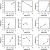 |
Fig. 14. Paths of three ETGs in the log(L)−log(σ), log(⟨I⟩e)−log(Re), and log(Re)−log(M*) planes. Blue dots give the position at redshift z = 4, green dots at z = 1, and red dots at z = 0. |
What appears to generate the observed tails, which we have identified as the SRs, seems more connected with the existence of the ZoE. When a galaxy reaches the passive state it can also fully relax and become virialized. The ZoE could therefore be a sort of universal limit established by the condition of full virialization and passiveness. The ZoE indicates that an object of a given mass can never have a radius smaller than that achieved when it reaches the undisturbed virialization and passive state. Since no system can cross the ZoE, this line appears as the physical driver of the log(⟨I⟩e)−log(Re) and log(Re)−log(M*) SRs. Only the systems that have reached a full virialization and are today evolving in a pure passive way can be distributed along the tails. The virial SRs with similar zero points seem to appear only when these conditions are met. This occurs for the massive galaxies that are today poorly affected by minor mergers (major mergers are very rare), so they are the systems closest to the condition of full virialization. They are also passive objects since their star formation quenched long time ago. For the objects of the ordinary family the virial equilibrium is very unstable since merging and stripping events and episodes of star formation rapidly move the galaxies toward a new condition of virial equilibrium. These systems are not passive yet, and are therefore far from the ZoE. In Paper III we will address the question of the ZoE in greater detail, examining the possible role played by cosmology.
Finally, we note that simulations show the formation of these tails only for galaxies with redshift z < 2. The tails are clearly visible at z = 0 only for massive systems. The log(Re)−log(M*) and log(⟨I⟩e)−log(Re) tails do not exist when z ≥ 2. We argue that the origin of these tails is the same for both planes. It is due to the progressive variation in homology of massive systems caused by the large number of dry merging events. These galaxies are almost passive and have developed a large extended stellar halo. Their Sérsic index is large, so that the combination of kv, σ, and M*/L in log scale progressively converges toward the limit of the ZoE. On the other hand, the small galaxies follow almost flat distributions in these planes at any redshift. The typical values of β for these systems is ∼3; they are objects moving along the slope of the observed FJ relation. Their dynamical status is continuously changed by interactions and feedback effects.
6. Conclusions
By exploiting the data of the WINGS and Omega-WINGS surveys we investigated the distribution of galaxies and GCs in the log(L)−log(σ), log(⟨I⟩e)−log(Re) and log(Re)−log(M*) planes. Then using the data extracted from the Illustris simulation, we compared the SRs resulting from the hydro-dynamical models with observations. In summary, these are our main conclusions:
− Galaxy clusters follow the same SRs of BCGs: their location in the log(L)−log(σ), log(⟨I⟩e)−log(Re), and log(Re)−log(M*) planes is that of very large, bright, and high velocity dispersion BCGs. In Paper I we noted that the normalized light profiles of galaxy clusters can be superposed on that of normal ETGs of intermediate luminosity. In this case, therefore, the parallelism with ETGs is with the brightest systems and not with the least luminous objects. From the equivalence of the normalized profiles it can be argued that the density distribution of galaxies in clusters is in some way similar to that of galaxies of intermediate or faint luminosity. Their structural parameters on the other hand are those of very bright and big BCGs. How can we explain this behavior? A possible answer is that the original mass profile of all these systems was approximately the same at earlier epochs (as we suggest in Paper I), but BCGs have progressively modified their profiles for the modifications induced by feedback effects and merging events. These modifications have not affected the GCs considered in our study. They are likely systems close to the virial equilibrium, with light profiles well fitted by a single Sérsic law. There are many nearby clusters (∼30%) still far from this condition that do not follow the same SRs of virialized clusters (see Cariddi et al. 2018). The transformation of the inner and outer density distribution of BCGs has probably no significant effects on the effective radius of these galaxies. This might occur if the mass fraction involved in the transformation is low in comparison with the total mass of the system. In Fig. 4 of Paper I we can see that the light profiles of faint and bright ETGs differ in the ranges r < 0.15Re and r > 2.5Re (i.e., in the zones including a small fraction of the total mass). The bulk of the mass (and consequently of the light) is contained in the interval 0.15 < r/Re < 2.5. The size of the effective radius depends on the bulk of the mass assembly and not on the mass involved in the transformation.
− The numerical simulations reproduce quite well the distribution of the BCGs and II-BCGs in the log(L)−log(σ), log(⟨I⟩e)−log(Re), and log(Re)−log(M*) planes, while they seem to fail for dwarfs and galaxy clusters. The effective radius deduced from the effective mass radius can still be a factor of ∼3 larger than observed for dwarfs. Simulated clusters are in general fainter and smaller in radius than real clusters. However, the well-known trends visible in the log(⟨I⟩e)−log(Re) and log(Re)−log(M*) planes made by bright galaxies are well reproduced. These relations appear as tails emerging from the flat distribution of less luminous galaxies. They appear after z ∼ 2 (i.e., after the epoch of maximum star formation) when systems progressively quenched. The real galaxies show that these trends are more clearly visible for galaxies in clusters than for objects in the field.
− The simulations indicate that each galaxy follows a complex path of evolution in the log(L)−log(σ), log(⟨I⟩e)−log(Re), and log(Re)−log(M*) planes. This path is due to the chaotic mass assembly history, made of merging, interaction–stripping events, vigorous star formation, and feedback effects. The most frequent paths determine the mean distribution observed in these planes. This behavior justifies the assumption of writing the log(L)−log(σ) relation in a new form, independent of the virial theorem:  law, where the slope β can assume either positive and negative values and
  is the key variable connected to the mass assembly and star formation history. The values of β fully constrain the slopes (i.e., the direction of motion) of galaxies in the SRs. Large negative values of β are those belonging to passive systems that naturally evolve toward progressively low values of the total luminosity. Most of the objects that are today in the tails of the distributions observed in the log(⟨I⟩e)−log(Re) and log(Re)−log(M*) planes have β < 0 (i.e., they are quenched passive systems). One should keep in mind that this relation is valid for a single galaxy.
− Both real and simulated data seem to show that there is a ZoE in the log(⟨I⟩e)−log(Re) and log(Re)−log(M*) planes, that is a region forbidden to any type of object. The origin of this empty region is not fully understood. No system can cross the ZoE. The slope and zero point of this line is the same for any kind of object, independent of its mass. We identified this line with the locus of fully virialized and passive objects. Galaxies progressively grow in mass and size across the cosmic epochs. After z ∼ 2, going toward the present, we observe in the simulations the formation of two tails in the log(⟨I⟩e)−log(Re) and log(Re)−log(M*) planes that indicate the existence of the ZoE. The most massive galaxies are the oldest virialized passive systems, so they are distributed almost along the ZoE. We have attributed the growth in mass and size of these systems to dry merging. Since the galaxies that follow the trend of the ZoE are in virial equilibrium, we argue that the dry merging events affecting these galaxies should involve small amount of mass that do not alter significantly the dynamical structure of the galaxies, but only the outer regions.
− Dwarf galaxies are not distributed along the ZoE; their effective radius does not scale linearly with the total stellar mass. This could be due to several reasons: the progressive large influence of DM; the effects of rotation; and the possibility that these systems are in a pseudo-virial condition, subject to transformation as soon as new mergers occur. It is possible that many of them have not yet reached the condition of virial passive evolution, so that their radius could be larger than expected on the basis of the full virialization. We know that in many of them star formation and galactic winds are still ongoing and many suffer strong interactions and merging with other galaxies of comparable mass in the clusters that might severely affect their dynamical equilibrium. Energy is continuously injected in these systems determining a larger radius. In conclusion, the zero point of the virial relation seems quite different for any object. We speculate that the systems that are still growing today will finally enter the tails of the bright virialized objects, while the dwarfs that do not grow anymore once the merging occurs are rare, and will progressively settle along the ZoE decreasing their radius. The simulations indicate that all systems evolve toward the virialization and passiveness.
− The distributions of objects observed in the log(L)−log(σ), log(⟨I⟩e)−log(Re), and log(Re)−log(M*) planes are connected to each other. The origin of the deviation from the trend predicted by the virial theorem is the same for all of them. Ultimately, it is due to a progressive variation in the mass-to-light ratio and homology induced by the large number of merging events experienced by galaxies. The small scatter suggests that a fine-tuning between structure and stellar population is in place.
Notably, in the log(⟨I⟩e)−log(Re) and log(Re)−log(M*) planes the presence of the ZoE is clearly visible, but does not appear in the log(L)−log(σ) plane. The simulations however suggest a small change in the slope of the relation for the brightest galaxies, i.e., for those entering the tails of the log(⟨I⟩e)−log(Re) and log(Re)−log(M*) relations. What is surprising is that despite the chaotic paths of evolution, the log(L)−log(σ) relation appears narrow at any epoch. The reason for this might reside in the moderate luminosity decrease with time of old stellar systems (the short steps in the total paths on the log(L)−log(σ) plane at nearly constant mass during which age effects can be seen). In addition, the sudden acquisition or loss of mass by mergers can change the mass and the stellar velocity dispersion relocating a galaxy in a different position along the plane (a merger of two galaxies with equal mass and luminosity generates an object two times brighter and more massive, i.e., ∼0.3 dex on both coordinates in the log(L)−log(σ) plane). This is almost equivalent to the spread observed in the relation. In other words it appears that the mass acquisition–loss acts like a razor ultimately shaping the log(L)−log(σ) distribution. The mass is the most important parameter determining the final luminosity and velocity dispersion of a galaxy.
Finally, we note that mergers and interactions drive the structural properties of the galaxies in the hierarchical scenario of galaxy formation and evolution, whereas the natural aging of the stellar populations plays a less relevant role. This role is quite evident at the present epoch when mergers are rare and a passive luminosity evolution takes place. On the other hand, in the early hierarchical or quasi-monolithic view of galaxy formation, mass and velocity dispersion are acquired very early and remain (nearly) constant, so that only the luminosity changes. For this reason we expect that the observed distribution of real galaxies in the log(L)−log(σ), log(⟨I⟩e)−log(Re), and log(Re)−log(M*) planes at increasing redshift will provide in the near future important information on the dynamical process of mass aggregation, structure formation, and evolution of the stellar population, and on the importance of feedback effects.
The more recent data of Illustris-TNG were not used, because they were only released when this work was almost completed.
Acknowledgments
We would like to thanks Prof. L. Secco and Dr. R. Caimmi for very useful clarifications about the Clausius’ Virial Theorem for multi-components systems. Finally, C.C. thanks the Department of Physics and Astronomy of the Padua University for the hospitality and computational support.
References
- Adami, C., Mazure, A., Biviano, A., et al. 1998, A&A, 331, 493 [Google Scholar]
- Bertelli, G., Bressan, A., Chiosi, C., Fagotto, F., & Nasi, E. 1994, A&AS, 106, 275 [NASA ADS] [Google Scholar]
- Bertelli, G., Girardi, L., Marigo, P., & Nasi, E. 2008, A&A, 484, 815 [NASA ADS] [CrossRef] [EDP Sciences] [Google Scholar]
- Bertelli, G., Nasi, E., Girardi, L., & Marigo, P. 2009, A&A, 508, 355 [NASA ADS] [CrossRef] [EDP Sciences] [Google Scholar]
- Bertin, G., Ciotti, L., & Del Principe, M. 2002, A&A, 386, 149 [NASA ADS] [CrossRef] [EDP Sciences] [Google Scholar]
- Bettoni, D., Kjærgaard, P., Milvan-Jensen, B., et al. 2016, The Universe of Digital Sky Surveys, 42, 183 [CrossRef] [Google Scholar]
- Biviano, A., Moretti, A., Paccagnella, A., et al. 2017, A&A, 607, A81 [NASA ADS] [CrossRef] [EDP Sciences] [Google Scholar]
- Bressan, A., Chiosi, C., & Fagotto, F. 1994, ApJS, 94, 63 [NASA ADS] [CrossRef] [Google Scholar]
- Bryan, G. L., & Norman, M. L. 1998, ApJ, 495, 80 [NASA ADS] [CrossRef] [Google Scholar]
- Caimmi, R. 2003, Astron. Nachr., 324, 250 [CrossRef] [Google Scholar]
- Caimmi, R. 2006, Serb. Astron. J., 174, 13 [CrossRef] [Google Scholar]
- Caimmi, R. 2009, New Astron., 14, 254 [CrossRef] [Google Scholar]
- Capaccioli, M., Caon, N., & D’Onofrio, M. 1992, MNRAS, 259, 323 [NASA ADS] [CrossRef] [Google Scholar]
- Cappellari, M., Scott, N., Alatalo, K., et al. 2013a, MNRAS, 432, 1709 [NASA ADS] [CrossRef] [Google Scholar]
- Cappellari, M., McDermid, R. M., Alatalo, K., et al. 2013b, MNRAS, 432, 1862 [NASA ADS] [CrossRef] [Google Scholar]
- Cariddi, S., D’Onofrio, M., Fasano, G., et al. 2018, A&A, 609, 133 [Google Scholar]
- Cava, A., Bettoni, D., & Poggianti, B. M. 2009, A&A, 495, 707 [NASA ADS] [CrossRef] [EDP Sciences] [Google Scholar]
- Chiosi, C., & Carraro, G. 2002, MNRAS, 335, 335 [NASA ADS] [CrossRef] [Google Scholar]
- Chiosi, C., Merlin, E., & Piovan, L. 2012, ArXiv e-prints [arXiv:1206.2532] [Google Scholar]
- Chiosi, C., Merlin, E., Piovan, L., & Tantalo, R. 2014, Galaxies, 2, 300 [CrossRef] [Google Scholar]
- Chiosi, C., Sciarratta, M., D’Onofrio, M., et al. 2017, ApJ, 851, 44 [NASA ADS] [CrossRef] [Google Scholar]
- Chiosi, C., D’Onofrio, M., Merlin, E., et al. 2020, A&A, submitted [arXiv:1908.08808] (Paper III) [Google Scholar]
- Dekel, A., & Birnboim, Y. 2006, MNRAS, 368, 2 [NASA ADS] [CrossRef] [Google Scholar]
- Djorgovski, S., & Davis, M. 1987, ApJ, 313, 59 [NASA ADS] [CrossRef] [Google Scholar]
- D’Onofrio, M., Fasano, G., Varela, J., Bettoni, D., et al. 2008, ApJ, 685, 875 [NASA ADS] [CrossRef] [Google Scholar]
- D’Onofrio, M., Bettoni, D., Bindoni, D., et al. 2011, Astron. Nachr., 334, 373 [NASA ADS] [CrossRef] [Google Scholar]
- D’Onofrio, M., Bindoni, D., Fasano, G., et al. 2014, A&A, 572, 87 [Google Scholar]
- D’Onofrio, M., Cariddi, S., Chiosi, C., et al. 2017, ApJ, 838, 163 [NASA ADS] [CrossRef] [Google Scholar]
- D’Onofrio, M., Sciarratta, M., Cariddi, S., et al. 2019, ApJ, 875, 103 (Paper I) [CrossRef] [Google Scholar]
- Dressler, A., Lynden-Bell, D., Bursten, D., et al. 1987, ApJ, 313, 42 [NASA ADS] [CrossRef] [Google Scholar]
- Dutton, A. A., van den Bosch, F. C., Faber, S. M., et al. 2011, MNRAS, 410, 1660 [NASA ADS] [Google Scholar]
- Faber, S. M. 1973, ApJ, 179, 731 [NASA ADS] [CrossRef] [Google Scholar]
- Faber, S. M., & Jackson, R. E. 1976, ApJ, 204, 668 [NASA ADS] [CrossRef] [Google Scholar]
- Fall, S. M., & Romanowsky, A. J. 2013, ApJ, 769, L26 [NASA ADS] [CrossRef] [Google Scholar]
- Fan, L., Lapi, A., Bressan, A., et al. 2010, ApJ, 718, 1460 [NASA ADS] [CrossRef] [Google Scholar]
- Fasano, G., Marmo, C., Varela, J., et al. 2006, A&A, 445, 805 [NASA ADS] [CrossRef] [EDP Sciences] [Google Scholar]
- Fasano, G., Vanzella, E., Dressler, A., et al. 2012, MNRAS, 420, 926 [Google Scholar]
- Feigelson, E. D., & Babu, G. J. 1992, ApJ, 397, 55 [NASA ADS] [CrossRef] [Google Scholar]
- Fraix-Burnet, D., D’Onofrio, M., & Marziani, P. 2019, A&A, 630, 63 [Google Scholar]
- Fritz, J., Poggianti, B. M., Bettoni, D., et al. 2007, A&A, 470, 137 [NASA ADS] [CrossRef] [EDP Sciences] [Google Scholar]
- Fritz, J., Poggianti, B. M., Cava, A., et al. 2011, A&A, 526, A45 [NASA ADS] [CrossRef] [EDP Sciences] [Google Scholar]
- Genel, S., Vogelsberger, M., Springel, V., et al. 2014, MNRAS, 445, 175 [Google Scholar]
- Genel, S., Nelson, D., Pillepich, A., et al. 2018, MNRAS, 474, 3976 [NASA ADS] [CrossRef] [Google Scholar]
- Girardi, L., Bertelli, G., Bressan, A., et al. 2002, A&A, 391, 195 [NASA ADS] [CrossRef] [EDP Sciences] [Google Scholar]
- Girardi, L., Grebel, E. K., Odenkirchen, M., & Chiosi, C. 2004, A&A, 422, 205 [NASA ADS] [CrossRef] [EDP Sciences] [Google Scholar]
- Graham, A. W. 2013, in Planets, Stars and Stellar Systems, eds. T. D. Oswalt, & W. C. Keel (Dordrecht: Springer Science-Business Media), 6, 91 [CrossRef] [Google Scholar]
- Gullieuszik, M., Poggianti, B. M., Fasano, G., et al. 2015, A&A, 581, 41 [Google Scholar]
- Hinshaw, G., Larson, D., Komatsu, E., et al. 2013, ApJS, 208, 19 [NASA ADS] [CrossRef] [Google Scholar]
- Kormendy, J. 1977, ApJ, 218, 333 [NASA ADS] [CrossRef] [Google Scholar]
- Lagos, C. D. P., Theuns, T., Schaye, J., et al. 2016, MNRAS, 459, 2632 [NASA ADS] [CrossRef] [Google Scholar]
- Lu, S., Dandan, X., Yunchong, W., et al. 2019, MNRAS, 492, 5930 [CrossRef] [Google Scholar]
- Magorrian, J., Tremaine, S., Richstone, D., et al. 1998, AJ, 115, 2285 [NASA ADS] [CrossRef] [Google Scholar]
- Merlin, E., & Chiosi, C. 2006, A&A, 457, 437 [NASA ADS] [CrossRef] [EDP Sciences] [Google Scholar]
- Merlin, E., & Chiosi, C. 2007, A&A, 473, 733 [NASA ADS] [CrossRef] [EDP Sciences] [Google Scholar]
- Merlin, E., Buonomo, U., Grassi, T., et al. 2010, A&A, 513, A36 [NASA ADS] [CrossRef] [EDP Sciences] [Google Scholar]
- Merlin, E., Chiosi, C., Piovan, L., et al. 2012, MNRAS, 427, 1530 [NASA ADS] [CrossRef] [Google Scholar]
- Moretti, A., Poggianti, B. M., Fasano, G., et al. 2014a, A&A, 564, 138 [Google Scholar]
- Moretti, A., Gullieuszik, M., Poggianti, B. M., et al. 2014b, A&A, 599, 81 [Google Scholar]
- Naab, T., Johansson, P. H., & Ostriler, J. P. 2009, ApJ, 699, L178 [NASA ADS] [CrossRef] [Google Scholar]
- Nelson, D., Pillepich, A., Genel, S., et al. 2015, Astron. Comput., 13, 12 [NASA ADS] [CrossRef] [Google Scholar]
- Pasetto, S., Grebel, E. K., Chiosi, C., et al. 2018, ApJ, 860, 120 [CrossRef] [Google Scholar]
- Pasquato, M., & Bertin, G. 2008, A&A, 489, 1079 [NASA ADS] [CrossRef] [EDP Sciences] [Google Scholar]
- Pignatelli, E., Fasano, G., & Cassata, P. 2006, A&A, 446, 373 [NASA ADS] [CrossRef] [EDP Sciences] [Google Scholar]
- Sanchez Almeida, J. 2020, MNRAS, 495, 78 [Google Scholar]
- Schaeffer, R., Maurogordato, S., Cappi, A., et al. 1993, MNRAS, 263, L21 [NASA ADS] [CrossRef] [Google Scholar]
- Sciarratta, M., Chiosi, C., D’Onofrio, M., & Cariddi, S. 2019, ApJ, 870, 70 [NASA ADS] [CrossRef] [Google Scholar]
- Secco, L., & Caimmi, R. 1992, ApJ, 395, 119 [CrossRef] [Google Scholar]
- Snyder, G. F., Torrey, P., Lotz, J. M., et al. 2015, MNRAS, 454, 1886 [NASA ADS] [CrossRef] [Google Scholar]
- Tantalo, R. 2005, Astrophys. Space Sci. Lib., 327, 235 [CrossRef] [Google Scholar]
- Tantalo, R., Chinellato, S., Merlin, E., Piovan, L., & Chiosi, C. 2010, A&A, 311, 361 [Google Scholar]
- Tully, R. B., & Fisher, J. R. 1977, A&A, 54, 661 [NASA ADS] [Google Scholar]
- Valentinuzzi, T., Woods, D., Fasano, G., et al. 2009, A&A, 501, 851 [NASA ADS] [CrossRef] [EDP Sciences] [Google Scholar]
- Valentinuzzi, T., Frits, J., Poggianti, B. M., et al. 2010, ApJ, 712, 226 [NASA ADS] [CrossRef] [Google Scholar]
- Varela, J., D’Onofrio, M., Marmo, C., et al. 2009, A&A, 497, 667 [NASA ADS] [CrossRef] [EDP Sciences] [Google Scholar]
- Vogelsberger, M., Genel, S., Springel, V., et al. 2014, Nature, 509, 177 [NASA ADS] [CrossRef] [Google Scholar]
- Zahid, H. J., Sohn, J., & Geller, M. J. 2018, ApJ, 859, 96 [CrossRef] [Google Scholar]
Appendix A: Two-component virial theorem and extended log(L)− log(σ) relation
The virial equations and the virial theorem for a composite system made of DM and BM can be derived for each component in presence of the tidal potential exerted by the other. We limit ourselves to the simplest case of two homogeneous concentric spherical subsystems made of DM and BM with isotropic stress tensor. The DM component has mass MDM and radius RDM The baryonic mass is supposed to be made of stars (and gas, which is neglected here), with total mass M* and radius Rs. Finally, the baryonic component is internal to the one made of dark matter.
Secco & Caimmi (1992) and Caimmi (2003, 2006, 2009) developed the virial equations for each subsystem taking into account the tidal potential exerted by the other component. We strictly follow their formalism. We start from the kinetic energies of the two components:
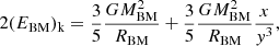 (A.1)
(A.1)
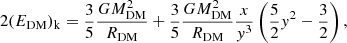 (A.2)
(A.2)
where
 (A.3)
(A.3)
and k stands for kinetic. In terms of the mass-weighted velocity dispersion, we obtain
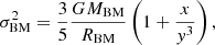 (A.4)
(A.4)
![Mathematical equation: $$ \begin{aligned}&\sigma _{\rm DM}^2 = \frac{3}{5} \frac{GM_{\rm DM}}{R_{\rm DM}} \left[1 + \frac{1}{x} \left(\frac{5}{2} - \frac{3}{2} \frac{1}{y^2} \right) \right]\cdot \end{aligned} $$](/articles/aa/full_html/2020/09/aa38221-20/aa38221-20-eq25.gif) (A.5)
(A.5)
The factor 3/5 in front of each term stems from the politropic description of the potential energy 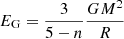 where n is the politropic index, which for a homogeneous distribution of mass is n = 0. The relations given by Eq. (A.5) represent the new virial conditions for an ideal composite galaxy made of DM and BM with concentric spherical and homogeneous distributions. These virial conditions are fully equivalent to the one in Eq. (1) and would immediately generate the relation of Eq. (2). The weakest issue of the above formalism is the assumption of homogeneity of the two subsystems. Nevertheless, for the use we are going to make of the above equations, this will be almost irrelevant.
To proceed further we need to know the fraction of BM originally in form of gas that is actually converted to stars. Numerical simulations of ETGs formation indicate that a large amount of gas is left over by the star formation activity and is heated up by feedback effects escaping the potential well in some cases. The typical star-to-gas ratio is ∼0.25 (Chiosi & Carraro 2002; Chiosi et al. 2012, 2014; Merlin & Chiosi 2006, 2007; Merlin et al. 2010, 2012).
Now we consider only the equations for the BM component, but limited to the stars:
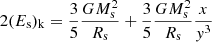 (A.6)
(A.6)
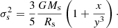 (A.7)
(A.7)
At this point, to arrive at the L − σ relation we follow a method different from the one used for Eq. (2). We look for the relationship between M* and Rs. To this end, we follow the formulation of the log(Re)−log(M*) relation developed by Fan et al. (2010). Assuming spherical symmetry for the sake of simplicity and the standard ratio MDM/MBM ≃ 6.6 ≡ x, the mass–radius relation for proto-galaxies made of DM and BM with total mass M = MDM + MBM ≃ 1.15 × MDM ≃ MDM for all practical purposes, is given by
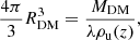 (A.8)
(A.8)
where ρ(z)∝(1 + z)3 is the density of the Universe at redshift z and λ the factor for the density contrast of the DM halo. This expression is of general validity, whereas the function λ depends on the cosmological model of the Universe (including the Λ-CDM case). All details can be found in Bryan & Norman (1998, their Eq. (6)).
In the context of Λ-CDM cosmology, Fan et al. (2010) have adapted Eq. (A.8) to provide a relationship between Rs and M*. They assume that over the Hubble time each halo that collapses at redshift zf generates a stellar mass M*. The stellar mass M* is then expressed by the ratio M* = MDM/θs, where θs is taken from numerical simulations of galaxy formation. Finally, the half-mass radius Rs is
 (A.9)
(A.9)
where Rs is in kiloparsecs.
As already anticipated, on average the efficiency of star formation is such that only a fraction of the original gas is converted to stars (typically one-fourth of it). Let us call this fraction Qs and consider it an adjustable parameter (i.e., QsMBM = M*). This quantity can soon be related to the ratio x of Caimmi (2003, 2006, 2009) and the parameter θs by θs = x/Qs. Another useful relation is θs = (MDM/MBM)/Qs, which for the assumed cosmology and efficiency of star formation gives θs ≃ 25. The quantity SS(nS) is a coefficient related to the Sérsic indexes nS and to the ansatz Rs = SS(nS)Rg relating gravitational and stellar mass radii, fs the velocity dispersion of the stellar component with respect to that of DM. All these quantities have been evaluated by Fan et al. (2010, to whom we refer for all the details): SS(nS) = 0.34, fs = 1. Also in this case the exact values for all these quantities are not mandatory here. It is worth noting that Eq. (A.9) links the stellar half-mass radius Rs to the mass MDM of its DM halo host.
We define now the three constants K1, K2, and Kσ:
 (A.10)
 (A.11)
![Mathematical equation: $$ \begin{aligned}&K_\sigma = \left[\frac{3}{5} \frac{G}{K_2 Q_{\rm s}} \right]\cdot \end{aligned} $$](/articles/aa/full_html/2020/09/aa38221-20/aa38221-20-eq33.gif) (A.12)
(A.12)
The half-mass radius Rs of Eq. (A.9) can be recast as
 (A.13)
and the velocity dispersion of the stars σs can be written as
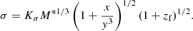 (A.14)
If we write M* as ΓL, where Γ is the stellar mean mass-to-light ratio, in logarithmic variables we obtain
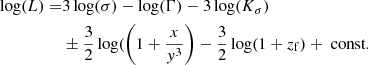 (A.15)
Equation (A.15) eventually takes a form mimicking the FJ relation. Here we see that the exponent of the σ term is now equal to 3 (instead of 2), which mirrors the slope of the assumed mass–radius relation of Eq. (A.9). There is a term containing the parameters x and y related to the presence of dark and baryonic matter, a term related to the galaxy formation redshift and a final const. that is related and fixed by the units adopted for the different quantities in usage.
Finally, we point out that in the case of MDM ≃ 0 (no dark matter) the parameter x → 0, Eq. (2) cannot be recovered because of the different power for the velocity dispersion and the term (1 + zf), which is not related to the presence of DM, but to the starting hypothesis of the proto-galaxy collapsing at redshift zf. If we drop it, or simply do not make it explicit, the formal recovery of Eq. (2) is straightforward.
In conclusion, the virial theorem of Eq. (1) and the log(L)−log(σ) relation of Eq. (2) should contain additional terms, and the general log(L)−log(σ) relation should be given in Eq. (A.15).
Appendix B: Model galaxies: bursts of star formation and mergers
In this section we briefly present the Monte Carlo method we used to describe bursts of star formation in galaxies of any mass, age, and mean metallicity and mergers among galaxies of different mass, age, and mean metallicity.
As a first step, we approximate the complex mix of stellar populations inside a galaxy of mass M with a SSP of suitable age TG, metallicity ZG, and the same mass. TG and ZG are the age and metallicity reached at the peak of star formation, which according to current galaxy models occurs shortly after the formation of the galaxy itself (Chiosi et al. 2017; Sciarratta et al. 2019) so that TG (zG) roughly corresponds to the formation time (redshift). With TU the present age of the Universe for the adopted cosmological scenario, then TG, z = TU − TG is the age (redshift) of the Universe when the galaxy was born.
In the following, we present two paradigmatic cases:
-
(i)
A galaxy already in place via the initial major episode of star formation, which later undergoes an additional episode of star formation of minor intensity (thereafter referred to as a burst case). With simulations of this kind, we explore the consequences of adding young stellar components to already evolved stellar assemblies; in other words, we can estimate the effect of a rejuvenation event on an otherwise passively evolving stellar system. This is the analog of simulating either completely wet mergers or a minor stellar activity for any internal reason (e.g., re-use of the gas shed by RGB and AGB stars).
-
(ii)
A merger of two galaxies of different mass, age, and metallicity. This would simply tell us how the photometric properties of each of the two subsystems added together would give rise to a new photometric appearance of the composed system even in absence of a companion star formation. This is the analog of a random combination of wet and dry mergers.
Bursts. The age TG of the initial star forming episode is supposed to fall in the age range TG, max > TG > TG, min. Subsequently, a burst of star formation engaging a certain percentage of the mass (typically up to about 10%) is supposed to occur at any age TB comprised between TB, max = TG, min and the present time (more precisely TB, min = 0.1 Gyr, the minimum age in the SSP grids).
The rest of the procedure is quite simple. First, we take the fluxes from SSPs of different metallicities, normalize them to unit of mass (with the Salpeter IMF and Ml = 0.1 M⊙ and Mu = 100 M⊙, MSSP = 5.826 M⊙), and then multiply them by the mass of the galaxy. Next, we randomize ages and masses of the seed SSP galaxies together with the age and mass percentages of the burst episode. To this end, it is more convenient to express the age and masses in terms of their logarithms, in order to avoid non-uniform distribution in the randomly chosen values. The ages (written in lower case symbols to remind the reader that they are expressed as logarithms) of the seed galaxies are given by
 (B.1)
(B.1)
and those of the bursts by
 (B.2)
(B.2)
r ∈ (0, 1) is a random, always different number. A similar procedure is followed for the mass of the seed SSP galaxy, which spans the range 107 − 1012 M⊙, and the mass percentage pB of the burst mass with respect to the mass of the host galaxy. The values of pB goes from 0% to 0.5%. Therefore, the relative contribution of the two components to the total flux (magnitudes in any pass-band) is given by

with obvious meaning of the symbols. Finally, since the SSP fluxes (magnitudes and colors) depend on both age and metallicity, and we know that this latter in turn increases with the galaxy mass, we have taken this into account by adopting an empirical mass–metallicity relation that is based on chemical models of galaxies and observational data and is presented here in Table B.1 taken from Sciarratta et al. (2019). Briefly, metallicity is binned in terms of logarithmic mass. Finally, for each burst the metallicity is for simplicity chosen to be equal to that of the seed galaxies. This means that, at variance with mergers, metallicities will not mix together.
Empirical mass–metallicity relation for SSP galaxies.
Mergers. The mass, metallicity, and age of each galaxy are derived using the same procedure as above, the only difference being that the permitted age interval now extends over nearly the whole Hubble time (i.e., TG, max − TG, min ≃ TG, max). Denoting with TG, j the age of the jth component of the merger (a single event for simplicity) and using the logarithmic notation, the ages tG, j are
 (B.3)
(B.3)
where r is the random number.
When two galaxies merge together, in the resulting bigger object there are stars from both initial components. At each time, their contribution to the total flux is first suitably shifted by the age difference between the two components to set up a common clock, and then weighed by the mass of each component. To keep our simulations simple, mergers occur between single pairs of galaxies, and the case of multiple mergers is not considered. Furthermore, we use only SSPs with solar partition of α-elements, i.e., [α/Fe] = 0.
All Tables
Coefficients of the log(L)−log(σ) relation with the different methods provided by the SLOPES program.
Different values of β and the corresponding slopes in the log(⟨I⟩e)−log(Re) and ⟨μ⟩e − log(Re) planes.
Slope and intercept of the best-fit log(Re)−log(M*) relation for different mass ranges.
Average and median values of β for the two intervals in cosmic epochs in the different mass ranges.
All Figures
|
Fig. 1. Left panel: distribution of ETGs and clusters in the log(L)−log(σ) plane. Black filled circles indicate our BCGs, red filled circles our II-BCGs, small gray filled circles the 1729 normal ETGs used by D’Onofrio et al. (2017) to study the FP, gray empty stars the faint ETGs of Bettoni et al. (2016), and blue filled circles our clusters. The normal ETGs reanalyzed in Paper I are not shown because their sigma values are not available. The black solid line gives the best fit of the whole dataset obtained with the orthogonal method. The dotted line shows the L ∝ σ2 law predicted for virial systems, while the dashed line gives the L ∝ σ4 FJ slope. Error bars are not shown because they are approximately as big as the plotted filled circles. Right panel: log(L)−log(σ) plane for real and simulated objects. The color-coding and symbols are the same as before. The open circles are used for simulated objects using the same color-coding. The plotted lines are the same as in the left panel. |
| In the text | |
|
Fig. 2. Left panel: distribution of galaxies and clusters in the log(⟨I⟩e)−log(Re) plane. Black filled circles indicate our BCGs, red filled circles our II-BCGs, green filled circles our random sample of normal ETGs, gray filled dots the 34982 galaxies analyzed by D’Onofrio et al. (2014) with GASPHOT, empty magenta stars the faint ETGs of Bettoni et al. (2016), and filled blue circles our clusters. The dashed line with slope −1 is that predicted for virialized systems for a possible ZoE. The zero point of this line was chosen as explained in Sect. 4.4. The dotted line is that expected for systems of equal luminosity MV = −21.5 with slope −2. The solid line with slope −1.2 is that obtained by Capaccioli et al. (1992). Right panel: log(⟨I⟩e)−log(Re) plane with real and simulated objects. The color-coding and symbols are the same as before. The open circles with the same colors of real galaxies are used for simulated objects. The plotted lines are the same as in left panel. |
| In the text | |
|
Fig. 3. Left panel: enlargement of the log(⟨I⟩e)−log(Re) plane with real and simulated galaxies. Black filled circles indicate our BCGs, red filled circles our II-BCGs, green filled symbols our random sample of normal ETGs, gray filled dots the WINGS ETGs of D’Onofrio et al. (2017), empty stars the faint ETGs of Bettoni et al. (2016), and filled circles our clusters. The small red dots are used for the whole set of Illustris galaxies at z = 0. In this case the effective mass radius is assumed to be equal to the effective radius. The dotted line is that expected for systems of luminosity MV = −21.5. Right panel: log(⟨I⟩e)−log(Re) plane for cluster (black dots) and non-cluster (red dots) ETGs. Shown is the subsample of galaxies with available masses from Fritz et al. (2007). In both panels the dashed lines are the trends for virialized systems with slope −1 and a zero point of a possible ZoE. |
| In the text | |
|
Fig. 4. Distributions in the log(Re)−log(M*) plane for normal ETGs (black filled circles), BCGs (green filled circles), and clusters of galaxies (blue filled circles) from our WINGS samples. The red small dots show the data of the Illustris simulations for galaxies at z = 0. The solid line is the fit of the galaxies and cluster sample, while the dashed line is the slope predicted from the virial theorem for a possible ZoE. |
| In the text | |
|
Fig. 5. Stellar mass–radius relation for galaxies in clusters (upper panel) and in the field (bottom panel). The open black circles show the real ETGs, the black filled circles the spiral galaxies, and the red dots the simulated data at z = 0. The stellar masses used here were derived from the K-band luminosity of our galaxies. |
| In the text | |
|
Fig. 6. log(Re)−log(M*) relation for ETGs and LTGs in clusters (left panels) and in the field (right panels). Galaxies are plotted in different colors according to their B − V color index. |
| In the text | |
|
Fig. 7. Upper panel: log(Re)−log(M*) plane. GCs are shown as magenta dots, dwarfs as green stars, normal ETGs as gray dots, BCGs as black dots, and clusters as blue dots. Each colored line indicates the average zero point of the systems calculated from Eqs. (1) and (5) with the values of kv, M*/L, and σ. The solid black line is obtained for the sample of galaxies and clusters taken together. All the lines have the slope 1 predicted for virialized systems. Lower panel: log(⟨I⟩e)−log(Re) plane. The same color-coding is adopted. Here the slope of the lines is −1. |
| In the text | |
|
Fig. 8. Stellar mass vs. difference in log units of the velocity dispersion measured from spectra and calculated through the virial equation. Upper panel: difference before the correction of the stellar mass. Lower panel: indicates that once the mass is corrected for the contribution of DM the two quantities are in good agreement (see text). Black dots are normal ETGs, green dots the faint ETGs measured by Bettoni et al. (2016), blue dots are galaxy clusters. |
| In the text | |
|
Fig. 9. Results of dissection of single bursts inside 13 Gyr SSP galaxies: evolution with time of Mv for the SSP galaxy with log M = 9 (Z = 0.004) perturbed by a single burst with mass fraction of 30%; solid thin curves are, in terms of increasing age, magenta (1 Gyr), blue (2 Gyr), and orange (7 Gyr); the thick black line is the unperturbed case shown for comparison. |
| In the text | |
|
Fig. 10. Simulations of the log(L)−log(σ) relation with the galaxies of the Illustris dataset at three different redshifts. Objects at z = 0 are shown as red dots, at z = 1 as green dots, and at z = 4 as blue dots. The colored lines show the best fits of the distributions and the resulting slopes are listed in the top left corner. |
| In the text | |
|
Fig. 11. Path of single galaxies in the log(L)−log(σ) plane from z = 4 (blue dot) to z = 0 (red dot). Within each box is the value of the slope β of the trajectory connecting the two epochs. |
| In the text | |
|
Fig. 12. Left panel: distribution of the slope β for the whole sample of galaxies. The red histogram shows the values of β measured from z = 4 to z = 1, the black histogram from z = 0.2 to z = 0. The dashed lines give the medians of the distributions. Right panel: distribution of the slope β for the galaxies of different masses. The red histogram shows the values of β measured from z = 4 to z = 0, the black histogram from z = 0.2 to z = 0. |
| In the text | |
|
Fig. 13. Four different paths in the log(⟨I⟩e) −log(Re) plane resulting from simulated data. Blue dots give the distribution at z = 4, green at z = 1, and red at z = 0. The half-mass radius in parsecs is assumed to be equal to the effective radius. The black lines connect the same object at different epochs. |
| In the text | |
|
Fig. 14. Paths of three ETGs in the log(L)−log(σ), log(⟨I⟩e)−log(Re), and log(Re)−log(M*) planes. Blue dots give the position at redshift z = 4, green dots at z = 1, and red dots at z = 0. |
| In the text | |
Current usage metrics show cumulative count of Article Views (full-text article views including HTML views, PDF and ePub downloads, according to the available data) and Abstracts Views on Vision4Press platform.
Data correspond to usage on the plateform after 2015. The current usage metrics is available 48-96 hours after online publication and is updated daily on week days.
Initial download of the metrics may take a while.