| Issue |
A&A
Volume 641, September 2020
|
|
|---|---|---|
| Article Number | A93 | |
| Number of page(s) | 28 | |
| Section | Atomic, molecular, and nuclear data | |
| DOI | https://doi.org/10.1051/0004-6361/202037948 | |
| Published online | 15 September 2020 | |
X-ray spectra of the Fe-L complex
II. Atomic data constraints from the EBIT experiment and X-ray grating observations of Capella
1
RIKEN High Energy Astrophysics Laboratory, 2-1 Hirosawa, Wako, Saitama, 351-0198, Japan
e-mail: This email address is being protected from spambots. You need JavaScript enabled to view it.
2
SRON Netherlands Institute for Space Research, Sorbonnelaan 2, 3584 CA Utrecht, The Netherlands
3
NASA/Goddard Space Flight Center, 8800 Greenbelt Rd, Greenbelt, MD 20771, USA
4
Max-Planck-Institut für Kernphysik, Heidelberg 69117, Germany
5
Department of Physics, University of Strathclyde, Glasgow G4 0NG, UK
6
Astronomical Institute “Anton Pannekoek”, University of Amsterdam, Science Park 904, 1098 XH Amsterdam, The Netherlands
7
INAF – IASF Palermo, Via U. La Malfa 153, 90146 Palermo, PA, Italy
8
MTA-Eötvös University Lendület Hot Universe Research Group, Pázmány Péter sétány 1/A, Budapest 1117, Hungary
9
Department of Theoretical Physics and Astrophysics, Faculty of Science, Masaryk University, Kotláská 2, Brno 611 37, Czech Republic
10
School of Science, Hiroshima University, 1-3-1 Kagamiyama, Higashi-Hiroshima 739-8526, Japan
11
Leiden Observatory, Leiden University, PO Box 9513 2300 RA Leiden, The Netherlands
12
Kavli Institute for the Physics and Mathematics of the Universe (WPI), University of Tokyo, Kashiwa 277-8583, Japan
13
ESTEC/ESA, Keplerlaan 1, 2201 AZ Noordwijk, The Netherlands
14
Laboratory of Instrumentation, Biomedical Engineering and Radiation Physics (LIBPhys-UNL), Department of Physics, NOVA School of Science and Technology, NOVA University Lisbon, 2829-516 Caparica, Portugal
15
Space Science Laboratory, University of California, Berkeley, CA 94720, USA
Received:
13
March
2020
Accepted:
8
July
2020
Abstract
The Hitomi results for the Perseus cluster have shown that accurate atomic models are essential to the success of X-ray spectroscopic missions and just as important as the store of knowledge on instrumental calibration and astrophysical modeling. Preparing the models requires a multifaceted approach, including theoretical calculations, laboratory measurements, and calibration using real observations. In a previous paper, we presented a calculation of the electron impact cross sections on the transitions forming the Fe-L complex. In the present work, we systematically tested the calculation against cross-sections of ions measured in an electron beam ion trap experiment. A two-dimensional analysis in the electron beam energies and X-ray photon energies was utilized to disentangle radiative channels following dielectronic recombination, direct electron-impact excitation, and resonant excitation processes in the experimental data. The data calibrated through laboratory measurements were further fed into a global modeling of the Chandra grating spectrum of Capella. We investigated and compared the fit quality, as well as the sensitivity of the derived physical parameters to the underlying atomic data and the astrophysical plasma modeling. We further list the potential areas of disagreement between the observations and the present calculations, which, in turn, calls for renewed efforts with regard to theoretical calculations and targeted laboratory measurements.
Key words: atomic data / methods: laboratory: atomic / techniques: spectroscopic / stars: coronae
© ESO 2020
1. Introduction
High-resolution X-ray spectroscopy provides unique opportunities for the exploration of both the microscopic physics of celestial bodies and the fundamental laws of cosmology. The observational window of X-ray spectroscopy, afforded by the spectrometers onboard Chandra, XMM-Newton, and Hitomi, will be fully open with the micro-calorimeters on the future XRISM and Athena missions. These telescopes will enable well-resolved spectroscopy of all kinds of cosmic X-ray sources, advancing the understanding into a broad range of physical conditions, from the heating source in the corona of a star to the formation of the largest scale baryonic structure.
The increasing sensitivity and resolving power of X-ray spectrometers require an accurate modeling of the X-ray spectra, which is, in turn, built on a range of fundamental atomic data, including mainly the wavelengths and cross-sections of radiative and collisional processes. The connection between X-ray astrophysics and atomic physics has never been so tight. The existing spectra already revealed the limits of the available atomic data, which are mostly obtained through theoretical calculations. The first Hitomi results on the Perseus cluster showed surprising discrepancies between the measurements using different atomic codes, for instance, 15% for the derived iron metallicity, while the statistical uncertainties from the observation are only 1% (Hitomi Collaboration 2018). These discrepancies represent systematic uncertainties that are even larger than the uncertainties due to the calibration of the Hitomi instruments. Another example showed that the laboratory measurements of the transition energies and cross sections of the oxygen innershell photoionization lines might be in tension with the results using the Chandra grating data, casting doubt on the interpretation of some of the observations (McLaughlin et al. 2017).
The Fe-L complex is a dominant feature in the X-ray spectra from many collisional plasma sources, such as stars, the interstellar medium, and groups of galaxies. The Fe-L complex is composed of a range of radiative transitions onto n = 2 states of Na-like to Li-like Fe ions, powered by multiple channels of collisional excitation, recombination, and ionization mechanisms. These Fe lines are very bright, making them key diagnostics for electron temperature, density, chemical abundances, gas motion, and photon scattering opacity of the sources (Phillips et al. 1996; Xu et al. 2002; Werner et al. 2006). Nevertheless, we lack adequate accuracy in the atomic data for the Fe-L complex (Gu et al. 2006a; Beiersdorfer et al. 2002, 2018; Brown et al. 2006; Bernitt et al. 2012; Mernier et al. 2018; Shah et al. 2019; Kühn et al. 2020), where the line formation is complicated. Unless the issue is addressed, the large errors in the data might potentially lead to unacceptable uncertainties in the future XRISM (Tashiro et al. 2018) and Athena (Barret et al. 2016) analysis.
In Gu et al. (2019; hereafter Paper I), we performed a distorted-wave calculation of the electron impact cross sections on the Fe-L ions, paying special attention to the resonant populating processes, including resonant excitation and dielectronic recombination. These calculations are systematically compared with the available R-matrix results, on both the collisional rates and the model spectra based on line formation calculation. We found that the two calculations agree within 20% on most of the main transitions, while the discrepancies become much larger for the weaker lines. Thus, the new Fe-L calculations must be verified before delivery to the community. This can be done by the systematic testing of the atomic data against (1) laboratory measurements using, for example, electron beam ion traps (EBITs) and (2) deep astrophysical observations of standard objects.
In the current paper, we first put forward an experimental benchmark using a recent EBIT measurement of the Na-like and Ne-like Fe lines (Sect. 2), focusing on the dielectronic recombination, along with direct and resonant excitation processes. In the second half, we implement the atomic data obtained through calculations and EBIT experiments into the analysis of the Capella grating data (Sect. 3). Similar work was done in Hitomi Collaboration (2018), in which the K-shell lines are directly calibrated against the Hitomi data of the Perseus cluster. Based on the above tests, we discuss potential areas of disagreement, as well as feasible corrections to the atomic data. Throughout the paper, the errors are given at a 68% confidence level.
2. Laboratory benchmark
2.1. Fe-L data measured with FLASH-EBIT
The experimental data used in the present analysis were reported by Shah et al. (2019; hereafter S19) using the FLASH-EBIT (Epp et al. 2010) facility located at the Max-Planck-Institut für Kernphysik in Heidelberg, Germany. In the experiment, a monoenergetic electron beam emitted from the hot cathode is compressed by a strong magnetic field of 6 T generated by superconducting Helmholtz coils. The electron beam collisionally ionizes Fe neutral atoms to the desired charge state, which are radially confined by the negative space charge potential of the electron beam and axially by electrostatic potentials applied to the set of drift tubes. The charge state distributions of the trapped ions are driven by electron-impact ionization, recombination, and excitation processes. The spontaneous radiative decay of excited states generates X-ray photons, which are collected at 90° to the electron beam axis with a silicon-drift detector (resolution ≈120 eV FWHM at 1 keV).
The line emission cross sections were measured for 3d−2p and 3s−2p channels of Fe XVII ions formed through dielectronic recombination, direct electron-impact excitation, resonant excitation, and radiative cascades (see terminology in Table 1). The experiment (S19) improves previous works by reducing the collision-energy spread to only 5 eV FWHM at 800 eV, which is six-to-ten times improvement compared to Brown et al. (2006), Gillaspy et al. (2011), and Beiersdorfer et al. (2017). Moreover, three orders of magnitude higher counting statistics allowed to distinguish narrow resonant excitation and dielectronic recombination features from direct excitation ones in the experiment. By comparing the laboratory line fluxes with a theoretical calculation tailored to match experimental conditions, S19 found good agreement with various theories for the 3s−2p transition, while accurately confirming known discrepancies in the 3d−2p transition. The latter was found to be overestimated by 9−20% by state-of-the-art-theories. This result is well in line with earlier lab measurements (Beiersdorfer et al. 2002; Brown et al. 2006).
Terminology of the relevant Fe XVII lines.
It remains unclear whether the same consistency and discrepancy can also be expected for the general spectral codes (e.g., AtomDB, Chianti, and SPEX) used in X-ray astronomy. In fact, these codes might behave differently from a dedicated calculation, as the database in the codes are often a combination of multiple sources of calculations, and are subject to various approximations. The main caveats for a direct EBIT-code benchmark are (1) cross sections in astronomical codes are often folded with the Maxwellian distribution, while these EBIT data were taken with a linear energy weighting; (2) conventional analyzing techniques cannot fully disentangle different radiative components (e.g., dielectronic recombination, radiative recombination, resonant excitation, direct excitation) when they overlap in beam energy in the EBIT data. The most obvious example is the complex around the beam energy ∼700−800 eV as shown in Fig. 1, where the strong dielectronic recombination transitions of the Na-like ions are mixed up with the resonant excitation and direct excitation transitions of the Ne-like ions; (3) most of the lines are blended in photon energy due to the poor X-ray resolution of the current data (Fig. 1). An accurate component study based on data decomposition and Maxwellianization (Sect. 2.2) is the key to solve these issues.
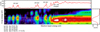 |
Fig. 1. EBIT X-ray data as a function of the electron beam energy (abscissa) and the photon energy (ordinate), corrected for the carbon foil transmission and the varying beam current. Color shows the number of counts. Photon energies of the main 3d−2p and 3s−2p transitions of Ne-like Fe are marked with the dashed lines. Upper and right panels: count profiles projected along the beam energy and the photon energy, respectively. |
Here we calibrate the EBIT data following the procedure in S19. First, the X-ray detector was shielded from the UV light by a 1 μm carbon foil, which also blocks a part of the X-ray radiation from the trap. The transmission of the thin foil was corrected based on the tabulated data from Henke et al. (1993), which gives 15% for 600 eV and 61% for 1000 eV. Second, the beam current Ie was adjusted as a function of beam energy E to keep the electron density  constant in the experiment, thus the space charge potential of the electron beam. The EBIT data was therefore corrected for the energy-dependent electron beam current density.
Finally, the X-ray polarizations from the radiative cascade and the cyclotron motion of electrons inside the electron beam were modeled based on the measurement and the theoretical procedure presented in Shah et al. (2018). The polarization calculations were performed using with the FAC code (Gu 2008) for each individual component, including dielectronic recombination, resonant excitation, and direct excitation, and presented in S19 as the machine-readable table (see data behind the Fig. 2 of S19). They also agree well with an independent experiment performed at LLNL EBIT, measuring X-ray line polarizations for Fe-L lines using the two-crystal technique (Chen et al. 2004). Moreover, in S19, a comprehensive agreement for various line emission cross sections at 90° was achieved using the FAC predictions (cf. Figs. 2−4 of S19). Two other completely independent experiments measuring the total dielectronic recombination cross sections the Test Storage Ring at Heidelberg (Schmidt et al. 2009) and the total direct excitation cross sections at LLNL EBIT (Brown et al. 2006) have also shown a good agreement with the S19 experimental data. Such extensive comparisons between independent theories and experiments in S19 provided us good confidence over the validity of the polarization predictions. We also note that the FAC polarization predictions are also thoroughly benchmarked in previous experiments at FLASH-EBIT (Shah et al. 2015, 2016, 2018; Amaro et al. 2017). Here, we inferred the total flux (Ftot) from the observed flux in the experiment (F90) through Ftot = 4πF90(3 − P)/3, where P is the degree of polarization. Based on FAC, the maximal effect of polarization is ∼40% for the dielectronic recombination and direct excitation at the 3d−2p manifold, and ∼5% for the direct excitation at the 3s−2p lines. The latter line complex is completely dominated by the radiative cascades thus depolarized (see Chen et al. 2004 and S19 for details). The systematic uncertainties on the polarization are expected to be minor when compared to the error items to be considered in Sect. 2.3.3.
2.2. Two dimensional fits
As shown in Fig. 1, the X-ray line emission of Ne-like and Na-like Fe is made up of two main components: the resonant X-ray peaks (including dielectronic recombination and resonant excitation) and the continuum (direct excitation and radiative recombination). An accurate determination of the transition intensities rests upon precise separation and extraction of each individual component, which is most related to two issues: (1) how to model the resonant component; and (2) how to separate the resonant and the continuum components.
To solve the first issue, we model the spectrum at the resonant X-ray peaks in two dimensions and extract each peak from its adjacent transitions. Following, for example, Li et al. (2013), the instrumental response is approximated using a set of semi-empirical equations,
 (1)
(1)
where the response functions of the full energy peak along the electron beam energy x and X-ray photon energy y are
 (2)
(2)
and
 (3)
(3)
The exponential tail function towards the low energy from the full peak is
 (4)
(4)
In the above equations, N1, N2, N3, and N4 are the normalization parameters, x0 and y0 are the excitation and photon energies of the transition, σx, σy, and  are the line spreads of the instrument, and Erfc is a complementary error function. All the parameters are left free for each X-ray peak. The Sherpa package1 (Freeman et al. 2001) in the CIAO software (Fruscione et al. 2006) is used to fit the EBIT data. To localize the noise analysis, the entire image is divided into several regions of interest (Fig. 2), and the fit is carried out independently for each region. The number of peaks are set by a visual inspection, unless an F-test determines that an additional resonant component is required. The quality of the fit to each region of interest is summarized in Table 2. Generally, the fit is robust, thanks to the very high count statistics and the excellent signal-to-noise (S/N) level of the data.
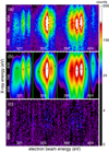 |
Fig. 2. (a) EBIT data of the dielectronic recombination from 3l3l′ states (where two electrons are excited to n = 3). (b) Best-fit model, the central position of each peak is marked by a black box. The boundaries of the regions of interest are shown by green lines. (c) Background noise and residual of the fit. |
Fit quality of the EBIT data.
As shown in Fig. 2, the dielectronic recombination of Na-like Fe from n = 3 levels are modeled using Eqs. (1)−(4). The overall reduced-χ2 is 1.2, for degrees of freedom of ∼22 000. The statistical uncertainties on the peak intensities are determined to be 1−4%, and the estimation of the relevant systematic uncertainties is described in Sect. 2.3.3. The average position accuracy is 0.5% on the beam energy and 3.5% on the photon energy, relative to the absolute values obtained from the fits.
A remaining issue is to separate the resonant and continuum components, especially for the 3s−2p line at beam energy >720 eV where the resonant excitation, dielectronic recombination, and direct excitation overlap. It is challenging to determine the resonant and continuum components simultaneously through fit, as their variations on the beam energy are both substantial. To overcome the degeneracy, we first fix the continuum spectrum to the theoretical value with the many-body perturbation theory (MBPT) method in the FAC code (Gu et al. 2006b; Gu 2009). The calculation has been described in S19 and benchmarked within the same experiment. A second-order MBPT algorithm and configuration interaction are used to enhance the accuracy of the atomic structure, which in the end has a direct effect on the collision strength of the allowed transitions. To minimize the discrepancy between theory and lab data, we scale the theoretical continuum spectra by the measurement data at beam energies of 1100−1115 eV, where the direct excitation dominates (Brown et al. 2006). As reported in S19 Table 1, the excitation continuum for the 3s−2p transition from the MBPT theory agrees with the EBIT data, while for the 3d−2p transition, the MBPT overestimates the continuum by ∼9%. Therefore, the scaling applied to the theoretical continuum has to be done separately for the two transitions. After further correcting for polarization and the instrumental broadening, the continuum model is subtracted from the original data, and the resonant peaks are modeled based on Eqs. (1)−(4). The continuum model can be updated by taking into account the residual from the resonant fits. Through four to five iterations, the procedure converges and the variation on the continuum flux between two runs becomes less than 10−4.
The continuum component is further decomposed into the 3s−2p lines and the 3d−2p lines. This is done in two steps, following a similar procedure to the one described in S19. First, we project the continuum data in the 700−1120 eV beam-energy band along the photon energy, and fit it with a two-component model, each with a form of  . The photon energies y0 of the two components are fixed at 0.826 keV (3d−2p) and 0.726 keV (3s−2p). Second, the 700−1120 eV electron beam band has further been divided into 14 segments, an independent two-component fit is done in each segment. Both components are treated as scale-down of the broad-band continuum,
 ![Mathematical equation: $ c[F_{y} (y) + F^{\ast}_{y} (y)] $](/articles/aa/full_html/2020/09/aa37948-20/aa37948-20-eq8.gif) , where c is the normalization factor. The parameters on the detector response (N2, N3, N4, σy, and
, where c is the normalization factor. The parameters on the detector response (N2, N3, N4, σy, and  ) are fully fixed to the results obtained in the first step. The line fluxes can thus be determined from the only free parameter c, which is obtained through a fit at each beam energy segment.
The decomposition of the EBIT data at the complex region (∼690−835 eV) is shown in Fig. 3. The dielectronic recombination from n = 6 and higher, and the resonant excitation from n = 3 and 4, are separated from the direct excitation continuum. The reduced-χ2 is ∼1.5 at the resonant peaks, where the systematic uncertainties are higher than those at the dielectronic recombination peaks (Sect. 2.3.3). Thanks to the very high counting statistics achieved in the experiment, the average position accuracy for the resonant components is 0.6% on the beam energy axis and 4% on the photon energy axis, relative to the absolute values obtained in the fits.
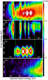 |
Fig. 3. (a) EBIT data of the complex region (labeled “DR + RE complex” in Fig. 1). (b) Model of dielectronic recombination, the central positions are marked by black boxes. The boundaries of the fit windows are shown by green lines. (c) Model of resonant excitation, the central positions are marked by black circles. (d) Background noise, residual of the fit, and the direct excitation continuum. |
To enable direct comparison with the astrophysical codes, we convolve the models of the resonant and the continuum components with a Maxwellian beam energy distribution. The line emissivities are calculated at four different temperatures, 0.25 keV, 0.5 keV, 0.75 keV, and 1.0 keV. Obviously, the Maxwellian distribution covers a broader energy range than the EBIT data. This would not affect the accuracy of the resonant component because most of the dielectronic recombination and resonant excitation transitions can be found in the EBIT scan range. However, the collision strength of direct excitation has a continuous distribution towards high energy (Paper I). To model the contribution beyond the EBIT scan range, we calculate the direct excitation cross section up to 10 keV based on the distorted-wave method implemented in the FAC code. To connect the calculation smoothly to the lab data, the FAC model is scaled to the polarization-corrected EBIT data at 1.1 keV. The line emissivities of direct excitation are obtained based on the combined EBIT data and the theoretical calculation. A direct calibration of the codes based on the Maxwellianized data is reported as follows.
2.3. Code calibration
The SPEX code calculates the ionization, recombination, and excitation processes on-the-fly from a database of fundamental atomic data, including the level energies, radiative transition probabilities, Auger rates, along with the excitation, ionization, and recombination rate coefficients. The atomic data used to calculate Ne-like Fe has been described in Paper I. In essence, the dielectronic recombination rates are obtained with a distorted wave calculation with the FAC code, while two parallel sets of excitation rate coefficients are available; one with the distorted wave method (SPEX-FAC hereafter) and the other one based on the R-matrix calculation reported in Liang & Badnell (2010) (SPEX-ADAS). For the Na-like Fe, the current atomic constants in the SPEX code are mostly computed with the FAC code. It includes complete 2s22p6nl, 2s22p5nln′ l′, and 2s2p6nln′l′ configurations with principal quantum number n and n′ ≤ 12. The full-order configuration mixing and relativistic Breit interaction are taken into account. The radiative relaxation routes and Auger routes for all the doubly-excited levels are calculated. The dataset is fed into the numerical solver for the rate equation in SPEX to calculate the steady-state level population, as well as the line emissivities from the individual (or a set of) atomic processes. We calculate the model spectra of dielectronic recombination into Na-like Fe and the resonant and direct excitation of the Ne-like Fe. A detailed comparison of the SPEX-FAC and SPEX-ADAS calculations is given in Sect. 3.3.
The experimental data are normalized to the model spectra at the dielectronic recombination transition from the intermediate state 2p53d2 (2F7/2). This line has excitation energy of 0.412 keV and photon energy of 0.816 keV. It is selected because this line is not only the strongest but also the simplest transition with the lowest allowed principal quantum number (n = 3) of all the related dielectronic recombination channels. The theoretical calculation is therefore expected to be reliable. The same normalization technique was applied in S19, in which it has been further verified through a set of consistency checks on the resonant excitation peak at 0.734 keV and on the radiative recombination continuum at 0.964 keV of beam energies. Moreover, a complete set of normalized experimental data has been also compared with the independent test storage ring experiment, both experiments agree very well (see Fig. 2 of S19). This shows the robustness of the calibration. The systematic uncertainty on the normalization factor has two main sources: the statistical uncertainty of 2% from the two-dimensional fit and the systematic error of 3% from the transmission curve of the carbon filter.
To have a crosscheck, we compare the dielectronic satellite intensities obtained from the two-dimensional fits with the data reported in S19, which were extracted from a strip region with a width of 60 eV around the photon energy of the 3d−2p line. The S19 data are reprocessed to have the same Maxwellian distribution and same beam energy resolution, and are normalized to our data at the 2p53d2 (2F7/2) transition. As seen in Fig. 4, the two data show roughly consistent relative heights of the n = 3−5 peaks, while our data show higher peaks at n = 6 and 7. Since the two data points are taken from a same experiment, this discrepancy must solely come from the data analysis. We speculate that, due to the poor resolution on photon energy, the conventional method adopted in S19 might miss a portion of flux, and the fraction included in the extraction region might vary among different dielectronic peaks. Furthermore, the heights of the peaks would look different with the conventional method if the resolution of beam energy varies during the energy scan. Our reconstruction from the two-dimensional fits should naturally be more accurate, as it could handle both the detector response and the possible beam energy width variation.
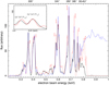 |
Fig. 4. Dielectronic recombination line intensities as a function of electron beam energy. The original SPEX model and the EBIT data are shown in black and red, respectively. Data uncertainties on the strong lines are marked as error bars alongside the peaks. Inset: normalization of the data and model at 2p53d2 (2F7/2). The resolutions of the spectra are 4 eV in the main plot, and 2 eV in the inset. For a comparison, the dielectronic recombination + direct excitation intensities reported in S19 are plotted in blue. The S19 data were extracted from a region of interest, with a width of 60 eV and centered on the 3d−2p transition energy. We convolve the S19 data with a Maxwellian beam energy distribution at 0.5 keV, and normalize the data to our curve shown in red at 2p53d2 (2F7/2). Direct excitation becomes gradually dominant at beam energy ≥0.8 keV in the S19 curve. |
2.3.1. Dielectronic recombination
Dielectronic recombination satellites are known to contribute significantly to the 3d−2p lines of Ne-like Fe (Beiersdorfer et al. 2017). Moreover, Beiersdorfer et al. (2018) found that the satellites provide an accurate diagnostic of the electron temperature. However, the scientific potential of the dielectronic satellites might be limited by the code accuracy; as shown in Fig. 4, when the SPEX model and experimental data (both with a Maxwellian temperature of 0.5 keV) are normalized at quantum number n = 3, the model clearly underestimates the line emissivities for n = 5 and higher. For n = 4 the model gives a reasonable fit to the data. To calibrate these satellites, we introduce a n-dependent tweak factor on the model spectra. First, the dielectronic satellites from the same n are grouped in both the data and the model. For each group with quantum number n, the Auger rates of the SPEX code are multiplied by a constant Cn to “fit” the observed EBIT spectrum. For Cn > 1, the dielectronic recombination rates increase, while the radiative branching ratios would decrease as more cascades become non-radiative. Taking these into account, the dielectronic recombination line strengths would increase by a factor of Cn(Ai + Rij)/(Rij + CnAi), where Ai is the original Auger rate from level i and Rij is the radiative decay rate from level i to j. The best-fit Cn factors are ∼1.5−2 for n = 5−8. For n = 9 and higher, the original Auger rates are multiplied by a factor of three to four. The large tweak factor at high n would not only lift the n = 9−12 peaks to the level of the EBIT data, but also can take into account the emission from n > 12 components, which are missing in the current code. For convenience, the missing fluxes from n > 12 are added to n = 9. Practically, the migration is valid because the n ≥ 9 peaks have nearly the same photon energy (δE/E ≤ 1 × 10⁻⁴), making it almost impossible to disentangle the n > 12 blend from the n = 9 transitions in astrophysical observations.
As shown in Fig. 5, the tweaked X-ray spectrum now matches well with the EBIT data. The discrepancy between model and data on the total flux has been reduced from 40% to ≤5%. Although this exercise is done only at a temperature of 0.5 keV, it is expected that the model spectra at other temperatures and ionization states are automatically corrected, as the underlying atomic data (i.e., Auger rate and transition probability) are similar. This is confirmed in Fig. 6, where the new SPEX model is compared with the EBIT data at 0.25, 0.5, 0.75, and 1.0 keV. The remaining discrepancies on the total fluxes are 4%, 4%, and 3% for 0.25 keV, 0.75 keV, and 1.0 keV. A minor caveat is that the line profiles of the SPEX and EBIT resonances might sometimes appear to be slightly different (Fig. 6). This is probably because even with the two-dimensional fits, it might still be difficult to fully separate the neighbouring resonances blended below the beam energy resolution.
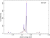 |
Fig. 5. X-ray spectra of Na-like Fe dielectronic recombination from SPEX with the original (black) and the corrected (blue) Auger rates, compared with the EBIT data (red), for a Maxwellian temperature of 0.5 keV. The spectral resolution is set to 2 eV. Note that the experimental photon energies obtained from 2D fits are corrected to the SPEX values, because the energy accuracy due to the detector resolution is poor compared to the theoretical values. |
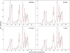 |
Fig. 6. Electron beam spectra of dielectronic recombination from SPEX (black) and EBIT (red), after the tweak factor Cn is applied to the SPEX code. Errors are plotted in the same way as in Fig. 4. In general the code agrees well with the EBIT data for the four temperatures shown. |
2.3.2. Direct and resonant excitations
Next, we compare the measurements of the direct and resonant excitation with the SPEX calculation on the 3d and 3s manifolds. It is well known that direct excitation and the following cascade are essential ingredients for both manifolds, while resonant excitation contributes mainly to the 3s levels (Doron & Behar 2002; Chen & Pradhan 2002; Brown et al. 2006; Shah et al. 2019). As found in Paper I, both 3lnl′ (n > 5) and 4lnl′ channels contribute to the resonant excitation; the former can be found at the complex region shown in Fig. 3, and the latter overlaps with the direct excitation continuum on the 3s band. In the SPEX code, these resonant channels are pre-calculated into an analytic form, which is combined on-the-fly with the direct excitation to determine the total rate coefficient.
Figure 7 plots the SPEX-EBIT comparison on the total fluxes for direct and resonant excitation. The 3d flux in the direct excitation continuum reveals an overestimation of the SPEX flux with distorted wave (R-matrix) calculations by 16(13)%. The difference is marginally significant with respect to the uncertainty of the EBIT measurement (Sect. 2.3.3). Similar discrepancies are reported in Loch et al. (2006), Chen (2011) with R-matrix approaches. As discussed in Gu (2009), Santana et al. (2015), and S19, the issue is likely rooted on the theoretical treatment of the high-order electron correlation, which mainly affects the transition probability and cross section of the 2p53d (1P1) level, and thus the 3C line emission at 15.01 Å. The other component in the 3d manifold, the 2p53d (3D1, so-called 3D) line seems to be better calculated (see Brown et al. 2006).
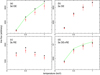 |
Fig. 7. Comparison of SPEX calculation and EBIT measurement on the Ne-like Fe excitation. (a) Direct excitation of the 3d manifold, (b) direct excitation of the 3s manifold, (c) resonant excitation onto the 3s levels, and (d) combined direct and resonant excitation of the 3s, from the original SPEX-FAC (black triangle), SPEX-ADAS (green line), and the EBIT experiment (red data). The SPEX-ADAS calculation does not separate direct and resonant excitation channels. |
The source composition of the 3s manifold is more complex than 3d. As reported in Paper I, cascades through the 3s−3p, 3s−3s, and 2s−2p transitions are the major routes. Direct excitation is the main process (70% at 0.8 keV) populating the upper states, while the rest is shared among the resonant excitation, dielectronic recombination, radiative recombination, and innershell ionization. Despite the intricate nature of the 3s manifold, the EBIT spectrum reveals a general agreement with the model for the direct and resonant excitation components (Fig. 7). The SPEX flux of direct excitation is consistent with the data within 7%. The resonant excitation based on the distorted wave calculation (Paper I) appears to be slightly overestimated, though the difference (11%) is marginal. The discrepancy becomes more subtle when the resonant excitation and direct excitation are combined in Fig. 7d, where a reasonable agreement within 8% is found.
For the code calibration, obviously, the primary issue would be to correct the atomic data on the 3C line at 15.01 Å. According to a previous EBIT result reported in Brown et al. (2001), the 3C/3D ratio is observed to be 3.04 ± 0.12 at high temperature where Ne-like Fe contributes 100% of the ion population. As shown in their Fig. 2, the observed intensity ratio can be interpreted by a relative cross section of the 3C and 3D continua equal to 3.0, which agrees well with the ratios found in other experiments (e.g., Brown et al. 2006; Kühn et al. 2020). This cross section ratio is then incorporated in the code calibration, combined with the results from the present EBIT experiments on the total 3C + 3D line intensity. As shown in Fig. 8, the 3C line emissivity of the Ne-like Fe is reduced by ∼20% from the original SPEX value. The new 3C + 3D intensity and the 3C/3D ratio are both in good agreement with the experimental values.
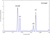 |
Fig. 8. X-ray spectrum of Ne-like Fe with the original SPEX-FAC rates (black) and the rates corrected by the EBIT data (blue), calculated for the equilibrium temperature of 0.5 keV. The spectral resolution is set to 2 eV. |
Combining the EBIT calibration to the Na-like and Ne-like transitions, we now obtain an update to the 17 Å-to-15 Å line ratio. This line ratio has broad astrophysical interests, in particular in the search for photon resonant scattering by ionized plasma (Xu et al. 2002; Beiersdorfer et al. 2002, 2004; Ogorzalek et al. 2017). The 17 Å line consists of two 3s transitions: 2s22p53s 1P1 (3G) and 2s22p53s 3P2 (M2) to the ground, and the 15 Å flux is contributed by the Ne-like 3C line and Na-like dielectronic recombination lines near 15.01 Å. As plotted in Fig. 9, the EBIT spectrum indicates a 17 Å-to-15 Å line ratio of 1.44 at 0.3 keV, and 1.29 at 1.0 keV. The line ratio with the original SPEX-FAC calculation is lower by 4−10%, within the uncertainty of the EBIT data. The small discrepancy between the two comes from the fact that the Na-like dielectronic recombination intensity increase (Sect. 2.3.1) has partially cancelled out the correction on the direct excitation for the Ne-like 3C line.
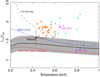 |
Fig. 9. Observed and calculated values of the 17 Å-to-15 Å line ratio as a function of temperature. The SPEX model calibrated by the EBIT data is plotted by a thick black solid line, and the uncertainty is shown by the grey band. The original SPEX-FAC calculation, the APEC v3.09, and the calibrated ratio with Ne-like Fe only are shown by the red solid, blue solid, and black dashed lines. The black triangle shows the laboratory measurement result taken from Beiersdorfer et al. (2004), and the magenta data points are the astrophysical measurements of elliptical galaxies taken from de Plaa et al. (2012). For NGC 5813, the deviation from the model curve is caused by the resonant scattering in the interstellar medium. The line ratios measured from the Chandra High-Energy Transmission Grating data of a sample of stellar coronae (Gu 2009) are shown in orange, and those measured with the XMM-Newton Reflection Grating Spectrometer for a sample of galaxies (Ogorzalek et al. 2017) are shown in cyan. |
We have further compared the EBIT line ratio with that from the APEC v3.0.9 database (Smith et al. 2001; Foster et al. 2012). The APEC model is systematically higher than the EBIT value, by 35% at 0.2 keV and 4% at 1.0 keV. This apparent discrepancy at low temperature likely comes from the dielectronic recombination calculation. The EBIT result is in agreement with the Tokamak measurement (Beiersdorfer et al. 2004) within their reported uncertainties.
It should be noted that the current EBIT experiment does not calibrate all the spectral components forming the 15 Å and 17 Å lines. An important missing component is the dielectronic recombination from F-like Fe, which contributes through radiative cascade to the 3s manifold. As shown in Paper I, the dielectronic recombination cascade contributes ∼35% of the M2 line at 1 keV, and is expected to be more important at higher energies. Besides, the current work does not cover the radiative recombination and innershell ionization components.
2.3.3. Experimental uncertainties
The overall uncertainties on the EBIT data are estimated as follows. Based on the two-dimensional fit, a statistical uncertainty on the normalization is calculated for each dielectronic recombination and resonant excitation peak (Tables A.1 and A.2). The statistical error is combined in quadrature with the systematic error on the transmission curve of the filter ∼3% as well as the systematic uncertainty on the normalization factor calculated at the transition 2p53d2 (2F7/2). As shown in Fig. 4, the errors on the dielectronic recombination resonances are 5−8% on the peaks with n = 3−10. For the resonant excitation, the average uncertainties on the total Maxwellianized fluxes are ∼9%.
Error sources on the direct excitation are (1) the statistical errors, in which the errors from the coupling of the 3d−2p and 3s−2p transitions are also taken into account, (2) 3% from the carbon foil transmission, (3) error on the normalization factor at 2p53d2 (2F7/2), and (4) the uncertainty on the theoretical calculation in the 1.1−10.0 keV band (Sect. 2.2). For the last component, we conservatively add a 12% uncertainty to the high beam energy band, which is determined by comparing the excitation cross sections obtained with the distorted wave and the MBPT methods at low beam energy band. Combining these components in quadrature gives a total error of ∼8% at 0.25 keV and ∼11% at 1 keV (Fig. 7).
3. Test on Capella grating data
An important aspect of the present work is implementing the new atomic calculations and the EBIT line measurement on the spectroscopy of representative astrophysical objects. To this end, we choose the bright non-degenerate stellar corona of the G1 + G8 binary Capella as the test target. The primary X-ray source is the quiescent coronal plasma, which is known to be in a quasi-collisional equilibrium state, heated to a temperature distribution over the range of 105−107 K (Dupree et al. 1993; Brickhouse et al. 2000; Phillips et al. 2001; Behar et al. 2001; Desai et al. 2005; Gu et al. 2006a; Gu 2009). The spectrum of the source shows a huge amount of emission lines from 1.5 to 175 Å, including Fe XVI and Fe XVII lines. As a calibration source for instrumental performances (in particular the resolving power, response matrix, and line spread function), Capella has been observed many times with X-ray grating spectrometers (Canizares et al. 2005). The very bright Fe-L lines, appropriate temperature, and extremely high-quality grating data in the archive make it the most suited target for the test.
The work is based on the Chandra High-Energy Transmission Grating (HETG) data, covering a wavelength range of 1.2−32 Å with a spectral resolution of 0.023 Å (∼1.2 eV at 800 eV, Medium Energy Grating) and 0.012 Å (∼34.7 eV at 6000 eV, High Energy Gratings). We do not include data from other instruments to minimize uncertainties from the cross-instrument calibration. A global, self-consistent fit is carried out for the broad HETG bandwidth, since the local fit (for instance, only in the 14−18 Å for Fe XVII) might miss features from complex astrophysical conditions (e.g., multi-temperature). As described below, the accurate calibration, as well as the completeness of the spectral modeling, are therefore essential to yield a reasonable description of the Capella spectrum using a global fit.
This section is organized as follows: first we describe the fit with the codes based on theoretical cross sections (Sects. 3.2 and 3.3), then we present the results with the EBIT-calibrated rate coefficients (Sect. 3.4). We present an overview of the atomic data constraints obtained for the most used plasma codes.
3.1. Data preparation
Archival Chandra HETG observations of Capella are summarized in Table 3. The total clean exposure time is 594.9 ks. A subset of the data has been reported in Phillips et al. (2001), Behar et al. (2001), Desai et al. (2005), and Gu et al. (2006a). The data were reduced using the CIAO v4.10 and calibration database (CALDB) v4.8. The chandra_repro script is used for the data screening and production of spectral files for each observation. The spectra and the associated response files are combined using the CIAO combine_grating_spectra tool. The Medium Energy Grating (MEG) spectrum in the wavelength range of 3−32 Å and the High Energy Gratings (HEG) spectrum in 1.5−3 Å are fit jointly.
Chandra ACIS/HETG observations of Capella.
3.2. Calibration and background
To remove possible residual calibration errors on the HETG effective area, we incorporate two correction functions in the spectral analysis. One represents uncertainty in the O I edge (22.6−22.9 Å), another is the possible error in the broad-band effective area of the X-ray mirrors. The edge correction is added as an extra neutral-O absorption component (hot model) in the spectral analysis. A positive (negative) absorption column density would mean that the actual edge is deeper (shallower) than the standard calibration. For the second component, we incorporate a knak component which determines the continuum correction function using piecewise power laws in the energy-correction factor space. The grid points are set at 1, 3, 6, 10, 14, 18, 26, 32, and 38 Å, skipping the location of O I edge that would be taken into account by the first component. By making several iterations between a fit with 100 eV-wide bins and a fit with the optimal binning, the best-fit knak and O I edge models are determined. The two components are fixed throughout the fits. The same approach was also used in the analysis of the Hitomi data of the Perseus cluster (Hitomi Collaboration 2018).
Shown in Fig. 10, the effective area correction factors derived with the knak model are compared with the empirical values obtained by a joint analysis of XMM-Newton and Chandra grating data for a sample of AGN sources (Kaastra, priv. comm.). Our models agree well with the data in 5−20 Å. At the longer wavelengths, the models seem to fall below the data, though the uncertainty of the data becomes larger.
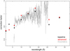 |
Fig. 10. Effective area correction factors from the baseline and the advanced fits shown in black and red data points, respectively. They are compared with the average effective area ratios between the XMM-Newton Reflection Grating Spectrometer and the Chandra Medium Energy Grating for a sample of AGN sources (Kaastra, priv. comm.). |
The shape of the lines are determined by the instrumental line spread function and the relevant astrophysical effects such as random motion, both components contain higher-order systematic uncertainties. The instrumental line spread function calibration has been cross-checked with the XMM-Newton Reflection Grating Spectrometer for a sample of bright sources, and a good match has been found between the two instruments (Kaastra, priv. comm.). Then, to model accurately the additional broadening from mainly the astrophysical effects, we incorporate the arbitrary line broadening model vpro, with a realistic profile shape calculated from the observed O VIII Lyα line at ∼19 Å. This model further allows fine-tuning on the line width with a Doppler parameter to eliminate the possible systematic uncertainties on the instrumental and astrophysical components.
The standard pipeline instrumental background has been reprocessed in the following way. A Wiener filter is applied to smooth out the noisy features in the background continuum, with the noise level determined by a Fourier transform. This process is needed for utilizing the C-statistic on the fits of spectra with low count numbers (Kaastra 2017).
3.3. Spectral modeling with theoretical rates
3.3.1. Atomic dataset
Here we describe the source of the fundamental atomic data used in the Capella work. The SPEX-ADAS database is utilized for the fit with the baseline model. It contains the same atomic data as the SPEX-FAC database except for the collisional excitation data on the Fe-L: the SPEX-ADAS incorporates the recent R-matrix results (Fe XVII from Liang & Badnell 2010, Fe XVIII from Witthoeft et al. 2006, Fe XIX from Butler & Badnell 2008, Fe XX from Witthoeft et al. 2007, Fe XXI from Badnell & Griffin 2001, Fe XXII from Liang et al. 2012, Fe XXIII from Fernández-Menchero et al. 2014, and Fe XXIV from Liang & Badnell 2011) for the low-lying levels (mostly up to n = 4), while the SPEX-FAC utilizes the uniform distorted wave calculation with isolated resonances from Paper I. The R-matrix and distorted wave calculations are found to be consistent within 20% on the main Fe-L lines, although the discrepancies become significantly larger for the weaker transitions, in particular for Fe XVIII, Fe XIX, and Fe XX. Generally speaking, the accuracy of R-matrix calculation is expected to be superior to that of the distorted wave with isolated resonances. At the high levels, the SPEX-ADAS and SPEX-FAC converge to the same distorted wave calculation, as the R-matrix data become gradually sparse with increasing n. The rates and wavelengths of non-Fe-L transitions in SPEX-ADAS and SPEX-FAC are the same as the public SPEX version 3.05. We also run the analysis with the standard SPEX version 3.05.
Though the atomic data incorporated in the APEC code are in general consistent with SPEX, significant differences on several individual transitions have been reported (Hitomi Collaboration 2018). We, therefore, include the latest APEC version 3.0.9 in the Capella fit, serving as an independent reference.
3.3.2. Baseline model
It is known that the X-ray spectra of stellar coronae require a differential emission measure modeling (Mewe et al. 2001). The multi-temperature structure of the coronal plasma can be well approximated by a combination of collisional ionization equilibrium (CIE) components. We define an optimal temperature grid of the model, derived from a pre-calculation of the ionic charge state as a function of equilibrium temperature. First, the average charge state C of each astronomically abundant element is calculated for a fine mesh of temperature T. We then obtain dT/dC at each temperature, and the minimal temperature change (in unit of keV) over all the abundant elements that brings one charge state further (δC = 1) can be approximated by
 (5)
(5)
This defines the most efficient temperature step size regarding the dependence on charge state. Based on Eq. (5), a set of 18 CIE components are defined within the temperature range of 0.1−10.0 keV. The emission measure of each component is free to vary, and the metal abundances of C, N, O, Ne, Mg, Al, Si, S, Ar, Ca, Cr, Fe, and Ni are also set as free parameters. The abundances of other elements (with weak lines) are set to the Solar ratio. All the CIE components are assumed to have the same set of abundances.
The interstellar absorption by neutral and ionized material is modeled using two hot components. The column densities of the two absorbers, and the temperature of the ionized component, are set free in the fits. The abundances of the absorbing materials are fixed to the Solar ratio.
We further apply a redshift component to the CIE components, and leave it as a free parameter to allow any residual uncertainties in the energy scale calibration, either of instrumental or astrophysical origin. Effective area correction components (Sect. 3.2) are also incorporated.
We use optimally binned spectra with the C-statistic. All abundances are relative to Lodders & Palme (2009) proto-solar abundances with free values relative to those abundances for the relevant elements. The ionization balance is set to the one in Urdampilleta et al. (2017).
The baseline model provides a reasonable fit to the main transitions in the Capella spectrum. For the weaker transitions, the fit becomes worse, probably due to the remaining uncertainties in the instrumental calibration and astrophysical effects, coupled with the unsolved issues with atomic data in the code. The total C-statistic value is 59 896 for an expected value of 7137, mostly due to the residuals in the weak lines (see detail in Appendix B). The fit is formally unacceptable, indicating that the current modeling of the complexity in the Capella spectrum is far from sufficient. Even so, it is still useful to discuss the relative changes of the C-statistic values, as well as the changes in plasma parameters, with respect to the baseline fit.
The differential emission measure distribution obtained with the baseline fit shows a primary peak at 0.51 keV, as well as secondary ones at 0.3 keV and 0.74 keV (Fig. 11). In general, it agrees with the previous measurements using the HETG instrument (e.g., Gu et al. 2006a). The elemental abundances also agree within the uncertainties with the values reported in Gu et al. (2006a), except for N and Si, which are derived to be ∼40% higher in our work.
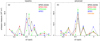 |
Fig. 11. Differential emission measure distributions with the baseline fits (a) and the advanced fits (b), using the atomic data from the SPEX-ADAS calculation (black), SPEX-FAC calculation (red), SPEX version 3.05 (green), and APEC (blue). The advanced fits with the EBIT correction are shown in dotted lines (they appear to nearly overlap with the non-EBIT-correction counterparts). The ultimate fit (see Appendix B for detail) is plotted in orange. |
As shown in Table 4, replacing the SPEX-ADAS calculation with the SPEX-FAC calculation in the baseline model yields a slightly better fit. The peak in emission measure distribution is shifted to 0.61 keV, which is likely a merge between the adjacent peaks at 0.51 keV and 0.74 keV (Fig. 11). The abundances remain nearly intact, except for Fe. It should be noted that any changes in non-Fe abundances are caused indirectly, as the rate coefficients of non-Fe species are the same in SPEX-ADAS and SPEX-FAC calculations.
Parameters of the reference model and sensitivity to model assumptions.
The quality of fit with both SPEX-ADAS and SPEX-FAC improves significantly from the one with SPEX version 3.05, proving that the new theoretical calculations are indeed better than those in the existing codes. There are multiple places where the parameters derived with SPEX-ADAS/FAC significantly differ from those with SPEX version 3.05. In particular, the Fe abundance with SPEX version 3.05 is 21% higher than the abundance with SPEX-ADAS, or 15% higher than the SPEX-FAC value, while the statistical uncertainty from the instrument is only 0.3%. This reconfirms the conclusion of Paper I that the new calculation tends to give lower Fe abundance than the standard SPEX code. The baseline fit with the latest APEC code is found worse than those with the calculations in SPEX. The emission measure distribution and elemental abundances are both significantly changed with APEC, reflecting the systematic uncertainties associated with the existing atomic codes.
3.3.3. Advanced model
As shown above, the baseline model should be regarded as a simple approximation to the astrophysical condition of the stellar corona. By properly incorporating several more degrees of freedom into the baseline model, we are able to achieve a more advanced physical description of the source.
We construct the advanced model as follows. First, the Fe abundance, which was tied among components in the baseline model, is now set free for all the CIE components with non-zero normalizations. The metallicities of a few components are tied to those of their adjacent components, as they cannot be determined independently with the current data. The C, N, O, Ne, Na, Mg, Al, Cr, and Ni abundances remain coupled, while the Si, S, Ar, and Ca abundances are tied for two groups of components, those with temperatures <1 keV and those above 1 keV. The model becomes quasi- multi-abundance, providing a better approximation to the possible metallicity gradient in the corona.
We further decouple the temperature used for ionization balance calculations, Tbal, from the temperature Tspec used for the evaluation of the emitted spectrum for the set of ionic abundances determined using Tbal. This is done by setting the rt = Tbal/Tspec a free parameter in the cie model. The rt parameter could take into account any possible minor non-equilibrium ionization effect, as well as the systematic uncertainties on the ionization and recombination rates and on the calibration of the broadband continuum (Hitomi Collaboration 2018).
Density diagnostics based on He-like triplets have been widely used for stellar sources (Ness et al. 2001; Mewe et al. 2001). As the efficiency of collisional deexcitation increases with density, the forbidden-to-intercombination line ratio is expected to be density-sensitive. Besides, the low-lying metastable levels might become significantly populated at high density, and the excitation, recombination, and radiative relaxation from or onto these levels are therefore required to reproduce the line emission (Badnell 2006). Spectra of C-like, B-like, and Be-like species are in particular sensitive to the electron density (Mao et al. 2017; Gu et al. 2019). These effects are taken into account in the advanced model by setting the plasma density as a free parameter.
The line broadening parameter v of the vpro model is set free for different temperature components. This allows extra uncertainties in the line spread function calibration, as well as in the modeling of the astrophysical turbulence in the multi-zone corona. The redshift component used for energy-scale calibration is also set free for different thermal components.
As shown in Table 4, the advanced model indeed improves the overall spectral fits. The different plasma codes converge to a similar form of the emission measure distribution, with a primary peak at 0.61 keV (Fig. 11). The advanced fit further leads to the changes of coronal abundances, by ≤30%, with respect to the baseline fit with the corresponding code.
As shown in Fig. 12, the Fe abundances change significantly as a function of temperature. The abundances of the 0.6−1.0 keV and <0.3 keV components are found to be about one solar or higher, while the abundances of other components are clearly sub-solar. On the other hand, advanced modeling is also used to constrain the mean electron density of the source. The upper limits on the density are obtained to be 0.6 × 109 cm−3 (SPEX-ADAS) and 1.4 × 109 cm−3 (SPEX-FAC). Our values agree with the previous results, for example, <2.4 × 109 cm−3 by Ness et al. (2001) and <7 × 109 cm−3 by Mewe et al. (2001). These results were derived from the O VII triplet line ratios measured with the Chandra Low Energy Transmission Grating Spectrometer (LETGS) data.
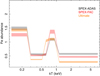 |
Fig. 12. Fe abundances as a function of temperature obtained with the advanced modeling, using the atomic data of SPEX-ADAS (black) and SPEX-FAC (red). The ultimate fit (see Appendix B) is shown in orange. |
In Appendix B, we present a semi-quantitative discussion on the fit quality with the advanced model. The SPEX-ADAS, SPEX-FAC, and APEC models are compared systematically, identifying key differences between calculations, as well as problem areas in the fit with each code. It reveals several issues on the wavelengths and line fluxes of the present calculations, which can be directly fed into the prioritization of future laboratory experiments. Both APEC and SPEX codes are in tension with the Capella data on wavelengths for about 10% of the observed lines. By fixing the apparent wavelength errors in the SPEX code and setting the central energies based on APEC or Chianti version 9.0 when these provide a better match to the data, we further improve the advanced model to its “ultimate” form shown in Table 4, Figs. 11 and 12. Details can be found in Appendix B and specifically Table B.2.
3.4. Results with EBIT-calibrated rates
The Fe XVII and Fe XVI rates corrected through the EBIT data (Sect. 2) are applied in the advanced fits. As shown in Table 4, the EBIT-corrected models yield slightly poorer fits than the models with theoretical rates, though the final differences in C-stat are small. Table 4 also tabulates the changes of the non-Fe abundances, mostly <10%, by incorporating the EBIT rates. The emission measure distributions using the EBIT rates remain nearly the same as using theoretical calculations presented earlier.
In Fig. 13, we take a detailed look at the Fe XVI and Fe XVII lines in the 15 Å and 17 Å regions, where the EBIT rates should affect the fit directly. The advanced models with EBIT rates and theoretical rates give nearly the same fit quality to the Fe XVII 3C and 3F lines at 15.01 Å and 16.78 Å, and the models with EBIT rates improve, though marginally, the fits to the 3D (15.26 Å), 3G (17.05 Å), and M2 (17.10 Å) lines. Note that these three lines are affected indirectly, as the EBIT rate is set only for the 3C transition (Sect. 2.3.2). Overall, the models with EBIT rates can provide a reasonable fit to the Fe XVII lines.
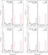 |
Fig. 13. Advanced fits shown in the wavelength ranges of 14.98−15.3 Å and 16.7−17.18 Å. The fits with SPEX-ADAS and SPEX-FAC calculations are plotted in panels a and c, and those with EBIT-calibrated rates are shown in panels b and d. Total model, Fe XVII transitions, and Fe XVI transitions are shown in black, red, and blue. Local C-stat values are given at the top. The total model is omitted in the 17 Å plot, as it would overlap with the Fe XVII lines. |
As shown in Fig. 13, the EBIT models appear to overestimate the Fe XVI dielectronic recombination lines near 15.03 Å. It seems that the Fe XVI lines from the original calculations already a bit exceed the observed level, and the EBIT rates make the discrepancy further larger. The Fe XVI lines likely contribute the main C-stat differences between the fits with the EBIT and theoretical models. However, considering that the Fe XVI line is only a weak transition with a much lower flux than its close neighbour, the fit of the line could have been affected by many systematic factors: a small error in the line spread function at the wing, non-Gaussianity, or an error in wavelength, might indirectly cause the poor fit. The line strength is also influenced by the determination of the ionization concentration and abundance of Fe XVI, for which there is a trade-off with the global fit of the broadband spectrum. Therefore, we cannot conclude based on the current fit that there is a real discrepancy between the EBIT and Capella observations on the Fe XVI lines.
We note that the current model seems to slightly underestimate the Fe XVII lines at 17 Å, in particular the M2 line, even though the direct and resonant excitation cross sections of the M2 and 3G lines are already verified with the EBIT data (Sect. 2.3.2), and the photon resonant scattering has been modeled with the hot component. A possible explanation is that these two lines are also significantly populated by the cascades following dielectronic recombination from Fe XVIII ions, which are missing in the current experiment (S19, Sect. 2.3.2). This calls for follow-up works on the dielectronic recombination contribution to the Ne-like lines at 17 Å.
4. Needs for benchmarks with laboratory data
Our fits to the Chandra grating spectrum of Capella not only revealed limits of the best available plasma codes but also showed the requirements for further testing of codes using high-accuracy laboratory measurements. In fact, a truly accurate fit to the Capella data requires a huge number of laboratory benchmarks, including transition energies and reaction rates of various processes, for both the L- and K-shells of all astrophysically relevant ions. While in practice such a complete test is not feasible, a few necessary tests, apart from the present study of the Fe XVII excitation and recombination (Sect. 2), should be prioritized.
First, the absolute cross section benchmarks for electron-impact excitation, resonant excitation, and dielectronic recombination followed by cascades, in particular for high-n states, for the remaining Fe-L ions, are probably of a high priority because they determine the intensities of most lines seen in the Capella spectrum. The accuracy of the cross section measurements is required to be better than 10%. These future measurements should be arranged with a full awareness of what is available at present: the IRON project with a series of theoretical and experimental works (following the first paper Hummer et al. 1993); individual EBIT works on excitation of Fe XVIII − Fe XXIV (Chen et al. 2006), Fe XXI − Fe XXIV (Chen et al. 2005), Fe XXIV (Chen et al. 2002; Gu et al. 1999), and Fe XXI − Fe XXIV (Gu et al. 2001) lines; storage ring measurements of dielectronic recombination forming Fe XVIII − Fe XXII (Savin et al. 2002a,b, 2003, 2006). Typical uncertainties on the measured cross section data are ∼10−25%. This can be improved for an example by implementing new measurement techniques at the EBIT, such as simultaneous X-ray observations with wide-band high-resolution transition-edge sensor microcalorimeters (Durkin et al. 2019; Szypryt et al. 2019) and polarization measurements (Shah et al. 2015, 2016, 2018) using dedicated X-ray polarimeters (Weber et al. 2015; Beiersdorfer et al. 2016). Further improvements can also be achieved by measuring the electron beam and ion cloud overlap in the EBIT (Liang et al. 2009; Arthanayaka et al. 2020).
Second, the wavelengths of strong lines need to be calibrated to an accuracy of the order of 0.01 Å. A list of tentative candidates, where wavelength mismatches between spectral codes and the Capella data are detected in the present work, can be found in Appendix B. Existing EBIT measurements using crystal spectrometers provided Fe-L wavelengths precise enough to allow reliable line identification (Brown et al. 1998, 2002). However, line energies can be significantly improved (to parts-per-million accuracy) by the application of resonant photoexcitation of highly charged ions using the EBIT at synchrotrons and free-electron lasers (Epp et al. 2007; Simon et al. 2010; Bernitt et al. 2012; Rudolph et al. 2013; Kühn et al. 2020). Besides line energies, these dedicated experiments can also provide accurate information on the radiative and auger decay rates (Steinbrügge et al. 2015; Togawa et al. 2020).
In addition, similar benchmarks using the laboratory data on the total ionization and recombination cross sections should be conducted, as they form the basis to determine the ionization balance as a function of electron temperature and density. These benchmarks will be utilized for further optimizing the quality of fits for the archival grating data from a variety of celestial sources. They are even more needed for XRISM and Athena with their superb sensitivity and large bandwidths.
5. Conclusion
We calibrate theoretical calculations of the Fe-L cross sections through EBIT measurements and Chandra grating observations of Capella. By utilizing a two-dimensional component analysis, the EBIT cross sections of dielectronic recombination from Na-like Fe, the resonant excitation, and the direct excitation of the Ne-like Fe are independently determined. We find reasonable agreement with the theoretical calculation for the excitation of the 3s−2p transitions, while the known discrepancies in the 3d−2p dielectronic recombination and direct excitation rates found in earlier works are confirmed with the new experimental data. The updated theoretical calculation and the EBIT results are then fed into global modeling of the Capella spectrum. The inclusion of the new atomic calculation improves significantly the fit to the observed spectrum, while the effect of the EBIT calibration remains inconclusive, in particular for the 3d−2p dielectronic recombination transitions, as it deeply couples with the astrophysical source modeling and instrumental calibration. However, the present work shows for the first time that the EBIT experimental data can be directly applied to benchmark and improve existing hot plasma models. Furthermore, future targeted EBIT experiments with the high-resolution photon detectors would certainly improve experimental accuracy that eventually will make models better. We conclude that the present Fe-L atomic calculation is almost ready to be delivered to the community, except for a few issues on wavelengths and rates, which are to be addressed with follow-up calculations and dedicated laboratory measurements.
Acknowledgments
L. Gu is supported by the RIKEN Special Postdoctoral Researcher Program. SRON is supported financially by NWO, the Netherlands Organization for Scientific Research. Work by C. Shah was supported by the Max-Planck-Gesellschaft (MPG), the Deutsche Forschungsgemeinschaft (DFG) Project No. 266229290, and by an appointment to the NASA Postdoctoral Program at the NASA Goddard Space Flight Center, administered by Universities Space Research Association under contract with NASA. P. Amaro acknowledges the support from Fundação para a Ciência e a Tecnologia (FCT), Portugal, under Grant No. UID/FIS/04559/2020(LIBPhys). J.M. acknowledges the support from STFC (UK) through the University of Strathclyde UK APAP network grant ST/R000743/1. The research leading to these results has received funding from the European Union’s Horizon 2020 Programme under the AHEAD2020 project (grant agreement n. 871158).
References
- Amaro, P., Shah, C., Steinbrügge, R., et al. 2017, Phys. Rev. A, 95, 022712 [CrossRef] [Google Scholar]
- Arthanayaka, T., Beiersdorfer, P., Brown, G. V., et al. 2020, ApJ, 890, 77 [CrossRef] [Google Scholar]
- Badnell, N. R. 2006, ApJS, 167, 334 [NASA ADS] [CrossRef] [Google Scholar]
- Badnell, N. R., & Griffin, D. C. 2001, J. Phys. B: At. Mol. Opt. Phys., 34, 681 [Google Scholar]
- Barret, D., Lam Trong, T., den Herder, J. W., et al. 2016, in SPIE Conf. Ser., Proc. SPIE, 9905, 99052F [Google Scholar]
- Behar, E., Rasmussen, A. P., Griffiths, R. G., et al. 2001, A&A, 365, L242 [NASA ADS] [CrossRef] [EDP Sciences] [Google Scholar]
- Beiersdorfer, P., Behar, E., Boyce, K. R., et al. 2002, ApJ, 576, L169 [NASA ADS] [CrossRef] [Google Scholar]
- Beiersdorfer, P., Bitter, M., von Goeler, S., & Hill, K. W. 2004, ApJ, 610, 616 [NASA ADS] [CrossRef] [Google Scholar]
- Beiersdorfer, P., Magee, E. W., Hell, N., & Brown, G. V. 2016, Rev. Sci. Instrum., 87, 11E339 [CrossRef] [Google Scholar]
- Beiersdorfer, P., Brown, G. V., & Laska, A. 2017, AIP Conf. Proc., 1811, 040001 [CrossRef] [Google Scholar]
- Beiersdorfer, P., Hell, N., & Lepson, J. K. 2018, ApJ, 864, 24 [CrossRef] [Google Scholar]
- Bernitt, S., Brown, G. V., Rudolph, J. K., et al. 2012, Nature, 492, 225 [NASA ADS] [CrossRef] [Google Scholar]
- Brickhouse, N. S., Dupree, A. K., Edgar, R. J., et al. 2000, ApJ, 530, 387 [NASA ADS] [CrossRef] [Google Scholar]
- Brown, G. V., Beiersdorfer, P., Liedahl, D. A., Widmann, K., & Kahn, S. M. 1998, ApJ, 502, 1015 [NASA ADS] [CrossRef] [Google Scholar]
- Brown, G. V., Beiersdorfer, P., Chen, H., Chen, M. H., & Reed, K. J. 2001, ApJ, 557, L75 [NASA ADS] [CrossRef] [Google Scholar]
- Brown, G. V., Beiersdorfer, P., Liedahl, D. A., et al. 2002, ApJS, 140, 589 [NASA ADS] [CrossRef] [Google Scholar]
- Brown, G. V., Beiersdorfer, P., Chen, H., et al. 2006, Phys. Rev. Lett., 96, 253201 [NASA ADS] [CrossRef] [PubMed] [Google Scholar]
- Butler, K., & Badnell, N. R. 2008, A&A, 489, 1369 [NASA ADS] [CrossRef] [EDP Sciences] [Google Scholar]
- Canizares, C. R., Davis, J. E., Dewey, D., et al. 2005, PASP, 117, 1144 [NASA ADS] [CrossRef] [Google Scholar]
- Chen, G. X. 2011, Phys. Rev. A, 84, 012705 [CrossRef] [Google Scholar]
- Chen, G. X., & Pradhan, A. K. 2002, Phys. Rev. Lett., 89, 013202 [NASA ADS] [CrossRef] [Google Scholar]
- Chen, H., Beiersdorfer, P., Scofield, J. H., et al. 2002, ApJ, 567, L169 [CrossRef] [Google Scholar]
- Chen, H., Beiersdorfer, P., Robbins, D., Smith, A., & Gu, M. 2004, Polarization measurement of Iron L-shell lines on EBIT-I, 87 [Google Scholar]
- Chen, H., Beiersdorfer, P., Scofield, J. H., et al. 2005, ApJ, 618, 1086 [CrossRef] [Google Scholar]
- Chen, H., Gu, M. F., Beiersdorfer, P., et al. 2006, ApJ, 646, 653 [CrossRef] [Google Scholar]
- de Plaa, J., Zhuravleva, I., Werner, N., et al. 2012, A&A, 539, A34 [NASA ADS] [CrossRef] [EDP Sciences] [Google Scholar]
- Desai, P., Brickhouse, N. S., Drake, J. J., et al. 2005, ApJ, 625, L59 [NASA ADS] [CrossRef] [Google Scholar]
- Doron, R., & Behar, E. 2002, ApJ, 574, 518 [NASA ADS] [CrossRef] [Google Scholar]
- Dupree, A. K., Brickhouse, N. S., Doschek, G. A., Green, J. C., & Raymond, J. C. 1993, ApJ, 418, L41 [NASA ADS] [CrossRef] [Google Scholar]
- Durkin, M., Adams, J. S., Bandler, S. R., et al. 2019, IEEE Trans. Appl. Supercond., 29, 2904472 [CrossRef] [Google Scholar]
- Epp, S. W., López-Urrutia, J. R. C., Brenner, G., et al. 2007, Phys. Rev. Lett., 98, 183001 [CrossRef] [PubMed] [Google Scholar]
- Epp, S. W., Crespo López-Urrutia, J. R., Simon, M. C., et al. 2010, J. Phys. B: At. Mol. Opt. Phys., 43, 194008 [CrossRef] [Google Scholar]
- Fernández-Menchero, L., Del Zanna, G., & Badnell, N. R. 2014, A&A, 566, A104 [NASA ADS] [CrossRef] [EDP Sciences] [Google Scholar]
- Foster, A. R., Ji, L., Smith, R. K., & Brickhouse, N. S. 2012, ApJ, 756, 128 [NASA ADS] [CrossRef] [Google Scholar]
- Freeman, P., Doe, S., & Siemiginowska, A. 2001, in SPIE Conf. Ser., eds. J. L. Starck, & F. D. Murtagh, Proc. SPIE, 4477, 76 [Google Scholar]
- Fruscione, A., McDowell, J. C., Allen, G. E., et al. 2006, in SPIE Conf. Ser., Proc. SPIE, 6270, 62701V [Google Scholar]
- Gillaspy, J. D., Lin, T., Tedesco, L., et al. 2011, ApJ, 728, 132 [NASA ADS] [CrossRef] [Google Scholar]
- Gu, M. F. 2008, Can. J. Phys., 86, 675 [NASA ADS] [CrossRef] [Google Scholar]
- Gu, M. F. 2009, ArXiv e-prints [arXiv:0905.0519] [Google Scholar]
- Gu, M. F., Kahn, S. M., Savin, D. W., et al. 1999, ApJ, 518, 1002 [NASA ADS] [CrossRef] [Google Scholar]
- Gu, M. F., Kahn, S. M., Savin, D. W., et al. 2001, ApJ, 563, 462 [CrossRef] [Google Scholar]
- Gu, M. F., Gupta, R., Peterson, J. R., Sako, M., & Kahn, S. M. 2006a, ApJ, 649, 979 [NASA ADS] [CrossRef] [Google Scholar]
- Gu, M. F., Holczer, T., Behar, E., & Kahn, S. M. 2006b, ApJ, 641, 1227 [NASA ADS] [CrossRef] [Google Scholar]
- Gu, L., Raassen, A. J. J., Mao, J., et al. 2019, A&A, 627, A51 [CrossRef] [EDP Sciences] [Google Scholar]
- Henke, B. L., Gullikson, E. M., & Davis, J. C. 1993, At. Data Nucl. Data Tables, 54, 181 [NASA ADS] [CrossRef] [Google Scholar]
- Hitomi Collaboration (Aharonian, F., et al.) 2018, PASJ, 70, 12 [NASA ADS] [Google Scholar]
- Hummer, D. G., Berrington, K. A., Eissner, W., et al. 1993, A&A, 279, 298 [NASA ADS] [Google Scholar]
- Kaastra, J. S. 2017, A&A, 605, A51 [NASA ADS] [CrossRef] [EDP Sciences] [Google Scholar]
- Kühn, S., Shah, C., López-Urrutia, J. R. C., et al. 2020, Phys. Rev. Lett., 124, 225001 [CrossRef] [Google Scholar]
- Li, Z., Tuo, X., Shi, R., & Zhou, J. 2013, Nucl. Sci. Tech., 24, 60206 [Google Scholar]
- Liang, G. Y., & Badnell, N. R. 2010, A&A, 518, A64 [NASA ADS] [CrossRef] [EDP Sciences] [Google Scholar]
- Liang, G. Y., & Badnell, N. R. 2011, A&A, 528, A69 [NASA ADS] [CrossRef] [EDP Sciences] [Google Scholar]
- Liang, G. Y., Crespo López-Urrutia, J. R., Baumann, T. M., et al. 2009, ApJ, 702, 838 [NASA ADS] [CrossRef] [Google Scholar]
- Liang, G. Y., Badnell, N. R., & Zhao, G. 2012, A&A, 547, A87 [NASA ADS] [CrossRef] [EDP Sciences] [Google Scholar]
- Loch, S. D., Pindzola, M. S., Ballance, C. P., & Griffin, D. C. 2006, J. Phys. B: At. Mol. Opt. Phys., 39, 85 [NASA ADS] [CrossRef] [Google Scholar]
- Lodders, K., & Palme, H. 2009, Meteorit. Planet. Sci. Suppl., 72, 5154 [Google Scholar]
- Mao, J., Kaastra, J. S., Mehdipour, M., et al. 2017, A&A, 607, A100 [NASA ADS] [CrossRef] [EDP Sciences] [Google Scholar]
- McLaughlin, B. M., Bizau, J. M., Cubaynes, D., et al. 2017, MNRAS, 465, 4690 [NASA ADS] [CrossRef] [Google Scholar]
- Mernier, F., de Plaa, J., Werner, N., et al. 2018, MNRAS, 478, L116 [NASA ADS] [CrossRef] [Google Scholar]
- Mewe, R., Raassen, A. J. J., Drake, J. J., et al. 2001, A&A, 368, 888 [NASA ADS] [CrossRef] [EDP Sciences] [Google Scholar]
- Ness, J. U., Mewe, R., Schmitt, J. H. M. M., et al. 2001, A&A, 367, 282 [NASA ADS] [CrossRef] [EDP Sciences] [Google Scholar]
- Ogorzalek, A., Zhuravleva, I., Allen, S. W., et al. 2017, MNRAS, 472, 1659 [NASA ADS] [CrossRef] [Google Scholar]
- Phillips, K. J. H., Bhatia, A. K., Mason, H. E., & Zarro, D. M. 1996, ApJ, 466, 549 [NASA ADS] [CrossRef] [Google Scholar]
- Phillips, K. J. H., Mathioudakis, M., Huenemoerder, D. P., et al. 2001, MNRAS, 325, 1500 [NASA ADS] [CrossRef] [Google Scholar]
- Rudolph, J. K., Bernitt, S., Epp, S. W., et al. 2013, Phys. Rev. Lett., 111, 103002 [NASA ADS] [CrossRef] [Google Scholar]
- Santana, J. A., Lepson, J. K., Träbert, E., & Beiersdorfer, P. 2015, Phys. Rev. A, 91, 012502 [CrossRef] [Google Scholar]
- Savin, D. W., Behar, E., Kahn, S. M., et al. 2002a, ApJS, 138, 337 [NASA ADS] [CrossRef] [Google Scholar]
- Savin, D. W., Kahn, S. M., Linkemann, J., et al. 2002b, ApJ, 576, 1098 [NASA ADS] [CrossRef] [Google Scholar]
- Savin, D. W., Kahn, S. M., Gwinner, G., et al. 2003, ApJS, 147, 421 [NASA ADS] [CrossRef] [Google Scholar]
- Savin, D. W., Gwinner, G., Grieser, M., et al. 2006, ApJ, 642, 1275 [NASA ADS] [CrossRef] [Google Scholar]
- Schmidt, E. W., Bernhardt, D., Hoffmann, J., et al. 2009, J. Phys. Conf. Ser., 163, 012028 [CrossRef] [Google Scholar]
- Shah, C., Jörg, H., Bernitt, S., et al. 2015, Phys. Rev. A, 92, 042702 [NASA ADS] [CrossRef] [Google Scholar]
- Shah, C., Amaro, P., Steinbrügge, R., et al. 2016, Phys. Rev. E, 93, 061201 [CrossRef] [Google Scholar]
- Shah, C., Amaro, P., Steinbrügge, R., et al. 2018, ApJS, 234, 27 [CrossRef] [Google Scholar]
- Shah, C., Crespo López-Urrutia, J. R., Gu, M. F., et al. 2019, ApJ, 881, 100 [CrossRef] [Google Scholar]
- Simon, M. C., Crespo López-Urrutia, J. R., Beilmann, C., et al. 2010, Phys. Rev. Lett., 105, 183001 [CrossRef] [Google Scholar]
- Smith, R. K., Brickhouse, N. S., Liedahl, D. A., & Raymond, J. C. 2001, ApJ, 556, L91 [NASA ADS] [CrossRef] [Google Scholar]
- Steinbrügge, R., Bernitt, S., Epp, S. W., et al. 2015, Phys. Rev. A, 91, 032502 [CrossRef] [Google Scholar]
- Szypryt, P., O’Neil, G. C., Takacs, E., et al. 2019, Rev. Sci. Instrum., 90, 123107 [CrossRef] [Google Scholar]
- Tashiro, M., Maejima, H., Toda, K., et al. 2018, Proc. SPIE, 10699, 1069922 [Google Scholar]
- Togawa, M., Kühn, S., Shah, C., et al. 2020, Phys. Rev. Lett., submitted [arXiv:2003.05965] [Google Scholar]
- Urdampilleta, I., Kaastra, J. S., & Mehdipour, M. 2017, A&A, 601, A85 [NASA ADS] [CrossRef] [EDP Sciences] [Google Scholar]
- Weber, S., Beilmann, C., Shah, C., & Tashenov, S. 2015, Rev. Sci. Instrum., 86, 093110 [CrossRef] [Google Scholar]
- Werner, N., Böhringer, H., Kaastra, J. S., et al. 2006, A&A, 459, 353 [NASA ADS] [CrossRef] [EDP Sciences] [Google Scholar]
- Witthoeft, M. C., Badnell, N. R., del Zanna, G., Berrington, K. A., & Pelan, J. C. 2006, A&A, 446, 361 [NASA ADS] [CrossRef] [EDP Sciences] [Google Scholar]
- Witthoeft, M. C., Del Zanna, G., & Badnell, N. R. 2007, A&A, 466, 763 [NASA ADS] [CrossRef] [EDP Sciences] [Google Scholar]
- Xu, H., Kahn, S. M., Peterson, J. R., et al. 2002, ApJ, 579, 600 [NASA ADS] [CrossRef] [Google Scholar]
Appendix A: EBIT line list
The energies and fluxes of the dielectronic recombination and resonant excitation peaks measured at the EBIT experiment (Sect. 2), as well as their statistical uncertainties determined from the two-dimensional fits, are listed in the following tables. The systematic uncertainties are given in Sect. 2.3.3.
EBIT dielectronic recombination line list.
EBIT resonant excitation line list.
Appendix B: Quality of the Capella fits
Figures B.1−B.3 show the full band Capella spectrum fit with advanced model using SPEX-ADAS (with the EBIT correction), and the relative differences of the fits from various atomic calculations. In Table B.1, we further evaluate the quality of the fits to the strong transitions (i.e., lines detected >5σ) in the data.
To summarize our findings in brief:
-
(1)
Table B.1 presents a detailed comparison of the present plasma code calculations for each strong line, reflecting the current knowledge and systematic uncertainties in the underlying atomic constants. It provides a list of problematic regions that would prioritize the dedicated laboratory measurements. Furthermore, the line-by-line evaluation of the model quality can be used as a reference in the future spectroscopic analysis with the XRISM and Athena data.
-
(2)
More than 60% of the observed transitions listed in Table B.1 are reasonably reproduced, both in wavelengths and line fluxes, by the SPEX-ADAS and SPEX-FAC calculations. This includes the main Fe-L transitions, such as the 15 Å and 17 Å Fe XVII lines. For 30% of the lines, the model fluxes (therefore the transition cross sections) are off by >20% from the values indicated by the data.
-
(3)
Both APEC and SPEX codes are in tension with the Capella data on wavelengths for about 10% of the observed lines. The SPEX code cannot fit the central energies of the Fe XVI line at 16.62 Å, Fe XVII lines at 11.03 Å, 13.12 Å, 13.82 Å and 16.24 Å, Fe XVIII lines at 10.36 Å, 10.54 Å, 11.33 Å, 11.43 Å, 14.53 Å, 15.49 Å, 15.63 Å, 16.07 Å, 17.36 Å, and 17.61 Å, Fe XIX lines at 9.84 Å, 10.81 Å, 13.49 Å, 13.63 Å, 13.93 Å, 16.11 Å, and 16.28 Å, Fe XX lines at 9.06 Å and 12.59 Å, Fe XXI line at 12.29 Å, Mg XI line at 7.85 Å, as well as a few Ni and Ca L-shell lines. The APEC code seems to match better for a few Fe lines, but it is off in several other transitions. As seen in the residual plots (Figs. B.1−B.3), these wavelength errors contribute substantially to the C-stat of the fits. It is therefore crucial to correct the wavelength database using data acquired in laboratory experiments as well as through advanced theoretical calculations.
-
(4)
There are potential line features in the spectrum, such as those at 9.62 Å, 9.79 Å, 9.89 Å, 14.41 Å, 17.8 Å, and 18.1 Å, which cannot be (fully) interpreted by the current model. A further study is required to identify the origin of these transitions.
-
(5)
Capella data provide an excellent test to a 0.6 keV plasma by resolving the Fe XVII transitions up to n = 8 and Fe XVIII transitions up to n = 5 (Table B.1). However, the L-shell emission of more ionized species, such as Fe XXI–Fe XXIV, are much weaker in the Capella data due to the drop in ionization concentration. Other astrophysical and laboratory sources are needed to calibrate these lines.
Capella line list.
By fixing the apparent wavelength errors in the SPEX code, we are able to obtain a final fit of the source spectrum. The central energies of the lines listed in item (3) above are set to the corresponding values in the APEC code, when APEC makes a better match. We further look into the Chianti database version 9.02 for the transitions where both APEC and SPEX wavelengths are off (see detail in Table B.2). Most of the wavelength errors are fixed by using the APEC and Chianti data, and the quality of the fit has been significantly improved (Table 4). Although the C-stat is formally still far from acceptable, this “ultimate” fit does represent the state-of-the-art understanding of the emission spectrum from the Capella corona. The obtained emission measure distribution (Fig. 11) and elemental abundances (Table 4) differ significantly from the advanced fits, suggesting that the accuracy of wavelengths does matter for the high-resolution spectroscopy.
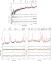 |
Fig. B.1. Chandra grating spectrum of Capella in 1.5−10.08 Å fit with different models. Upper panels in each subfigure: show fit with the advanced SPEX-ADAS model with EBIT calibration (red). Middle panels: fit residual with the advanced models (grey points), as well as the ratio between the SPEX-FAC fit and the SPEX-ADAS fit in black, and the APEC-to-SPEX-ADAS ratio in orange. Lower panels: fit residual with the ultimate model. |
Wavelength correction for the ultimate modeling.
All Tables
All Figures
|
Fig. 1. EBIT X-ray data as a function of the electron beam energy (abscissa) and the photon energy (ordinate), corrected for the carbon foil transmission and the varying beam current. Color shows the number of counts. Photon energies of the main 3d−2p and 3s−2p transitions of Ne-like Fe are marked with the dashed lines. Upper and right panels: count profiles projected along the beam energy and the photon energy, respectively. |
| In the text | |
|
Fig. 2. (a) EBIT data of the dielectronic recombination from 3l3l′ states (where two electrons are excited to n = 3). (b) Best-fit model, the central position of each peak is marked by a black box. The boundaries of the regions of interest are shown by green lines. (c) Background noise and residual of the fit. |
| In the text | |
|
Fig. 3. (a) EBIT data of the complex region (labeled “DR + RE complex” in Fig. 1). (b) Model of dielectronic recombination, the central positions are marked by black boxes. The boundaries of the fit windows are shown by green lines. (c) Model of resonant excitation, the central positions are marked by black circles. (d) Background noise, residual of the fit, and the direct excitation continuum. |
| In the text | |
|
Fig. 4. Dielectronic recombination line intensities as a function of electron beam energy. The original SPEX model and the EBIT data are shown in black and red, respectively. Data uncertainties on the strong lines are marked as error bars alongside the peaks. Inset: normalization of the data and model at 2p53d2 (2F7/2). The resolutions of the spectra are 4 eV in the main plot, and 2 eV in the inset. For a comparison, the dielectronic recombination + direct excitation intensities reported in S19 are plotted in blue. The S19 data were extracted from a region of interest, with a width of 60 eV and centered on the 3d−2p transition energy. We convolve the S19 data with a Maxwellian beam energy distribution at 0.5 keV, and normalize the data to our curve shown in red at 2p53d2 (2F7/2). Direct excitation becomes gradually dominant at beam energy ≥0.8 keV in the S19 curve. |
| In the text | |
|
Fig. 5. X-ray spectra of Na-like Fe dielectronic recombination from SPEX with the original (black) and the corrected (blue) Auger rates, compared with the EBIT data (red), for a Maxwellian temperature of 0.5 keV. The spectral resolution is set to 2 eV. Note that the experimental photon energies obtained from 2D fits are corrected to the SPEX values, because the energy accuracy due to the detector resolution is poor compared to the theoretical values. |
| In the text | |
|
Fig. 6. Electron beam spectra of dielectronic recombination from SPEX (black) and EBIT (red), after the tweak factor Cn is applied to the SPEX code. Errors are plotted in the same way as in Fig. 4. In general the code agrees well with the EBIT data for the four temperatures shown. |
| In the text | |
|
Fig. 7. Comparison of SPEX calculation and EBIT measurement on the Ne-like Fe excitation. (a) Direct excitation of the 3d manifold, (b) direct excitation of the 3s manifold, (c) resonant excitation onto the 3s levels, and (d) combined direct and resonant excitation of the 3s, from the original SPEX-FAC (black triangle), SPEX-ADAS (green line), and the EBIT experiment (red data). The SPEX-ADAS calculation does not separate direct and resonant excitation channels. |
| In the text | |
|
Fig. 8. X-ray spectrum of Ne-like Fe with the original SPEX-FAC rates (black) and the rates corrected by the EBIT data (blue), calculated for the equilibrium temperature of 0.5 keV. The spectral resolution is set to 2 eV. |
| In the text | |
|
Fig. 9. Observed and calculated values of the 17 Å-to-15 Å line ratio as a function of temperature. The SPEX model calibrated by the EBIT data is plotted by a thick black solid line, and the uncertainty is shown by the grey band. The original SPEX-FAC calculation, the APEC v3.09, and the calibrated ratio with Ne-like Fe only are shown by the red solid, blue solid, and black dashed lines. The black triangle shows the laboratory measurement result taken from Beiersdorfer et al. (2004), and the magenta data points are the astrophysical measurements of elliptical galaxies taken from de Plaa et al. (2012). For NGC 5813, the deviation from the model curve is caused by the resonant scattering in the interstellar medium. The line ratios measured from the Chandra High-Energy Transmission Grating data of a sample of stellar coronae (Gu 2009) are shown in orange, and those measured with the XMM-Newton Reflection Grating Spectrometer for a sample of galaxies (Ogorzalek et al. 2017) are shown in cyan. |
| In the text | |
|
Fig. 10. Effective area correction factors from the baseline and the advanced fits shown in black and red data points, respectively. They are compared with the average effective area ratios between the XMM-Newton Reflection Grating Spectrometer and the Chandra Medium Energy Grating for a sample of AGN sources (Kaastra, priv. comm.). |
| In the text | |
|
Fig. 11. Differential emission measure distributions with the baseline fits (a) and the advanced fits (b), using the atomic data from the SPEX-ADAS calculation (black), SPEX-FAC calculation (red), SPEX version 3.05 (green), and APEC (blue). The advanced fits with the EBIT correction are shown in dotted lines (they appear to nearly overlap with the non-EBIT-correction counterparts). The ultimate fit (see Appendix B for detail) is plotted in orange. |
| In the text | |
|
Fig. 12. Fe abundances as a function of temperature obtained with the advanced modeling, using the atomic data of SPEX-ADAS (black) and SPEX-FAC (red). The ultimate fit (see Appendix B) is shown in orange. |
| In the text | |
|
Fig. 13. Advanced fits shown in the wavelength ranges of 14.98−15.3 Å and 16.7−17.18 Å. The fits with SPEX-ADAS and SPEX-FAC calculations are plotted in panels a and c, and those with EBIT-calibrated rates are shown in panels b and d. Total model, Fe XVII transitions, and Fe XVI transitions are shown in black, red, and blue. Local C-stat values are given at the top. The total model is omitted in the 17 Å plot, as it would overlap with the Fe XVII lines. |
| In the text | |
|
Fig. B.1. Chandra grating spectrum of Capella in 1.5−10.08 Å fit with different models. Upper panels in each subfigure: show fit with the advanced SPEX-ADAS model with EBIT calibration (red). Middle panels: fit residual with the advanced models (grey points), as well as the ratio between the SPEX-FAC fit and the SPEX-ADAS fit in black, and the APEC-to-SPEX-ADAS ratio in orange. Lower panels: fit residual with the ultimate model. |
| In the text | |
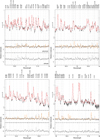 |
Fig. B.2. Same as Fig. B.1, but in 10.08−18 Å. |
| In the text | |
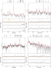 |
Fig. B.3. Same as Fig. B.1, but in 18−32 Å. |
| In the text | |
Current usage metrics show cumulative count of Article Views (full-text article views including HTML views, PDF and ePub downloads, according to the available data) and Abstracts Views on Vision4Press platform.
Data correspond to usage on the plateform after 2015. The current usage metrics is available 48-96 hours after online publication and is updated daily on week days.
Initial download of the metrics may take a while.