| Issue |
A&A
Volume 640, August 2020
|
|
|---|---|---|
| Article Number | A82 | |
| Number of page(s) | 22 | |
| Section | Interstellar and circumstellar matter | |
| DOI | https://doi.org/10.1051/0004-6361/201834377 | |
| Published online | 14 August 2020 | |
Constraining MHD disk winds with ALMA
Apparent rotation signatures and application to HH212
1
Leiden Observatory, Leiden University,
PO Box 9513,
2300
RA Leiden, The Netherlands
e-mail: This email address is being protected from spambots. You need JavaScript enabled to view it.
2
Observatoire de Paris, PSL University, Sorbonne Université, CNRS, LERMA,
75014
Paris,
France
3
Univ. Grenoble Alpes, CNRS, IPAG,
38000
Grenoble, France
4
Université Paris-Saclay, CNRS, Institut d’Astrophysique Spatiale,
91405 Orsay, France
5
Laboratoire de Physique de l’ENS, ENS, Université PSL, CNRS, Sorbonne Université, Université Paris-Diderot,
Paris, France
6
INAF, Osservatorio Astrofisico di Arceti, Largo E. Fermi 5,
50125
Firenze, Italy
7
IRAM, 300 rue de la piscine,
38406,
Saint Martin d’Hères, France
8
Laboratoire d’Astrophysique de Bordeaux, Université de Bordeaux, CNRS, B18N, Allée Geoffroy Saint-Hilaire,
33615
Pessac, France
Received:
4
October
2018
Accepted:
16
March
2020
Abstract
Context. Large millimeter interferometers (ALMA, NOEMA, SMA), with their high spectral resolution and sensitivity, are revealing a growing number of rotating outflows, which are suggested to trace magneto-centrifugal disk winds (MHD DWs). However, the angular momentum flux that they extract and its impact on disk accretion are not yet well quantified.
Aims. We aim to identify systematic bias in the process of retrieving the true launch zone, magnetic lever arm, and associated angular momentum flux of an MHD DW from apparent rotation signatures, as measured by observers from position-velocity (PV) diagrams at ALMA-like resolution.
Methods. We constructed synthetic PV cuts from self-similar MHD DW solutions over a broad range of parameters. We examine three methods for estimating the specific angular momentum jobs from PV cuts: the “double-peak separation” method (relevant for edge-on systems), and the “rotation curve” and “flow width” methods (applicable at any view angle). The launch radius and magnetic lever arm are then derived from jobs through the widely used theory of MHD flow invariants, and are compared to their true values on the outermost streamline. Predictions for the “double-peak separation” method are tested on published ALMA observations of the HH212 rotating SO wind at resolutions from ~250 au to ~18 au.
Results. The double-peak separation method and the flow width method provide only a lower limit to the true outer launch radius rout. This bias is mostly independent of angular resolution, but increases with the wind radial extension and radial emissivity gradient and can reach a factor of ten. In contrast, the rotation curve method leads to a good estimate of rout when the flow is well resolved, and an upper limit at low angular resolution. The magnetic lever arm is always underestimated due to invisible angular momentum stored as magnetic field torsion. ALMA data of HH212 confirm our predictions of the bias associated with the double-peak separation method, and the large rout ≃ 40 au and small magnetic lever arm first suggested by Tabone et al. (2017, A&A, 607, L6) from PV cut modeling. We also derive an analytical expression for the fraction of disk angular momentum extraction performed by a self-similar MHD disk wind of given radial extent, magnetic lever arm, and mass ejection-to-accretion ratio. The MHD DW candidate in HH212 extracts enough angular momentum to sustain steady accretion through the whole disk at the current observed rate.
Conclusions. The launch radius estimated from observed rotation signatures in an MHD DW can markedly differ from the true outermost launch radius rout. Similar results would apply in a wider range of flow geometries. While in principle it is possible to bracket rout by combining two observational methods with opposite bias, only comparison with synthetic predictions can properly take into account all observational effects, and also constrain the true magnetic lever arm. The present comparison with ALMA observations of HH212 represents the most stringent observational test of MHD DW models to date, and shows that MHD DWs are serious candidates for the angular momentum extraction process in protoplanetary disks.
Key words: stars: protostars / ISM: jets and outflows / ISM: individual objects: HH212 / magnetohydrodynamics (MHD) / accretion, accretion disks
© ESO 2020
1 Introduction
A major enigma in our understanding of the structure and evolution of protoplanetary disks (PPDs) is the exact mechanism by which angular momentum is extracted to allow disk accretion onto the central object at the observed rates, which are much faster than expected for microscopic collisional viscosity (e.g., Hartmann et al. 2016). The problem is particularly emphasized during the early protostellar phase (so-called Class 0) where the second hydrostatic Larson’s core must grow in less than 105 yr to stellar masses by accretion of disk material. One possible mechanism, first introduced by Blandford & Payne (1982) in the context of active galactic nuclei and shown to be particularly efficient, involves the vertical removal of angular momentum by the twisting of large-scale poloidal magnetic field lines; the angular momentum is then carried away in a magneto-centrifugal disk wind (MHDDW), becoming collimated into a jet on a large scale. The same process was first proposed by Pudritz & Norman (1983) to explain bipolar jets and outflows from young stars, and by Konigl (1989) to explain their correlation with accretion luminosity. The ability of a resistive Keplerian accretion flow to feed a steady, super-Alfvénic MHD DW was further demonstrated through semi-analytical works and numerical simulations (see e.g., Ferreira 1997; Pudritz et al. 2007, and references therein). An alternative well-studied mechanism able to transfer angular momentum and drive accretion through PPDs is the magneto-rotational instability (MRI Balbus & Hawley 1991). However, recent nonideal MHD calculations and simulations reveal that the MRI is quenched in the outer regions of PPDs around 1–20 au (the so-called “dead zone”), and MHD DWs are being revived as prime candidates to induce disk accretion through these outer regions (see e.g., Turner et al. 2014; Bai 2017; Béthune et al. 2017, and references therein). Therefore, robust observational diagnostics of the presence and radial extent of MHD DWs in young stars is crucially needed to fully understand the physics of PPDs, and of planet migration inside them (see e.g., Ogihara et al. 2018).
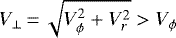
In this context, the outermost launching radius of the MHD DW (denoted as rout in the following) is a particularly important parameter to determine. A key observational diagnostic for constraining the range of launch radii is the specific angular momentum carried by the wind (Bacciotti et al. 2002; Anderson et al. 2003; Ferreira et al. 2006). In particular, Anderson et al. (2003) showed that in a steady, axisymmetric, and dynamically cold (negligible enthalpy) MHD DW, the launch radius r0 of a given wind streamline is related to its kinematics through what we refer to hereafter as “Anderson’s relation”:
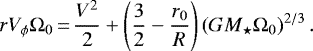 (1)
(1)
Here, r denotes the distance from the axis at the observed wind point, Vϕ the azimuthal velocity, V the total velocity modulus, R the distance to the central star, M⋆ the stellar mass, and 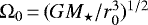 the Keplerian angular velocity at r0. The term in (r0∕R) accounts for gravitational potential at low altitudes, which are starting to be probed with ALMA. This relation further shows that a cold, steady axisymmetric MHD DW must everywhere rotate in the same sense as the disk (i.e., Vϕ Ω0 > 0). We note that an MHD DW could still be counter-rotating if it is not dynamically cold, that is, enthalpy-driven rather than magnetically driven1 (see also Sauty et al. 2012), non-steady (Fendt 2011), or non-axisymmetric (Staff et al. 2015). However, in none of these cases would it be possible to infer r0 from the above relation2.
The first tentative jet rotation signatures were uncovered in optical forbidden lines at the base of atomic T Tauri jets thanks to the unprecedented angular resolution of the HubbleSpace Telescope (HST) in the form of centroid velocity differences ≃ 10−20 km s−1 between opposite edges of the flow. In two cases (DG Tau, CW Tau), the inferred jet rotation sense agrees with the disk rotation sense, as required by Anderson’s formula for a cold, steady, axisymmetric MHD DW. The inferred values of launch radii r0 range from 0.2 to 3 au, and the estimated total angular momentum flux represents 60–100% of that required for accretion through the underlying disk, consistent with the MHD DW scenario (Bacciotti et al. 2002; Anderson et al. 2003; Coffey et al. 2007). In a more detailed modeling analysis, Pesenti et al. (2004) showed that the spatial pattern of velocity shifts along and across the DG Tau jet is in excellent agreement with synthetic predictions for an extended MHD DW launched out to 3 au. However, at flow radii smaller than the PSF diameter, velocity shifts are strongly reduced dueto beam convolution. As most atomic T Tauri jets are not well transversally resolved even with HST, this effect might explain why their rotation is still so difficult to detect at the limited spectral resolution (≃50 km s−1) of current optical and near-infrared 2D spectro-imagers. The reduced rotation shifts in narrow jets by smearing effects also makes them more susceptible to contamination by external asymmetries, possibly explaining the occurrence of “counter-rotating” cases (RW Aur, RY Tau, Th 28, Cabrit et al. 2006; Coffey et al. 2015; Louvet et al. 2016).
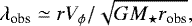
The unique combination of high spectral resolution (< 1 km s−1), sensitivity, and angular resolution provided by large millimeter interferometers such as PdBI/NOEMA, SMA, and ALMA is now allowing thedetection of much weaker rotation signatures than in the optical range, through velocity differences of only a fraction of a kilometer per second between opposite sides of the flow axis. Consistent rotation signatures in the same sense as the underlying disk have thus been uncovered in a growing number of molecular jets and/or outflows from protostars: CB 26 (Launhardt et al. 2009), Ori-S6 (Zapata et al. 2010), DG Tau B (Zapata et al. 2015; de Valon et al. 2020), TMC1A (Bjerkeli et al. 2016), Orion Source I (Hirota et al. 2017), HH212 (Tabone et al. 2017; Lee et al. 2017a, 2018a), HH211 (Lee et al. 2018b), HH30 (Louvet et al. 2018), and IRAS4C (Zhang et al. 2018). Standard application of Anderson’s formula to the observed rotation signatures yields “observed” DW launch radii robs ranging from 0.05 to25 au.
When discussing the implications of these results, for example to favor an X-wind (Shu et al. 2000) over an extended MHD DW, it is generally assumed that robs derived in this way is close to the outermost launch radius rout. However, it is important to realize that they are in general two different things.
A detailed fitting of ALMA data in HH212 by MHD DW models required much larger outer launch radii than inferred by Anderson’s formula, namely rout ≃ 40 au instead of robs ≃ 1 au for the SO-rich slow outflow, and rout ≃ 0.2−0.3 au instead of robs ≃ 0.05 au for the SiO-rich jet (Tabone et al. 2017). Hence, even at the high resolution achievable with ALMA, it appears that application of Anderson’s formula to the “observed” angular momentum can lead to significant underestimation of the true outermost launching radius of an MHD DW, at least in some cases.
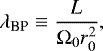
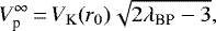
Another key parameter of an MHD DW that we wish to estimate from observations is the magnetic lever arm parameter λBP, which measures the total specific angular momentum extracted by the wind in units of the initial Keplerian value (Blandford & Payne 1982). An estimate of λBP is necessary to assess angular momentum extraction by the wind. Observational estimates of λBP are generally obtained through (see e.g., Anderson et al. 2003)
 (2)
(2)
where robs is the launch radius inferred using Anderson’ formula. However, the few detailed comparisons with MHD DW models favor λBP values that are two to three times larger than this (Pesenti et al. 2004; Tabone et al. 2017).
Understanding and quantifying these observational biases in rout and λBP is crucial if we want to be able to infer robust constraints on the role of MHD DWs in sustaining accretion across PPDs. This question was first addressed by some of us in the specific case of HST optical observations of the DG Tau atomic jet (Pesenti et al. 2004). The goal of the present paper is to readdress this issue in the new context of ALMA-like spectral resolution for wind parameters relevant to current molecular disk wind candidates. We therefore compute synthetic predictions for self-similar MHD DW models at resolutions typical of current millimeter interferometers, and apply the same methods as observers to estimate the wind launch radius and magnetic lever arm parameter, which are then compared with the true rout and λBP in the model. Quasi-edge-on DWs are studied in particular detail, as their rotation shifts are maximized by projection effects, and have the interesting property of being independent of angular resolution.
Our main predictions in the quasi-edge-on case are checked against published ALMA data of HH212 ranging in resolution from 250 to 18 au, which represent the most stringent test of MHD DWs to date. We also derive an analytical expression for the fraction of disk angular momentum flux extracted by any self-similar MHD DW, and apply it to HH212 for illustration.
The paper is laid out as follows: in Sect. 2, we present self-similar MHD DW solutions used for building our synthetic predictions. In Sect. 3, we describe the effect of model parameters on rotation signatures, and three methods used by observers to estimate the flow specific angular momentum from them. We then examine in representative cases how the launch radius and magnetic lever arm parameter deduced with Anderson’s relations differ from the true rout and λBP. In Sect. 4, we compare our predictions for the edge-on case with ALMA observations of HH212, and we examine angular momentum extraction by the proposed MHD disk wind model. In Sect. 5, we summarize our results and their implications for ALMA-like observations of molecular MHD DW candidates in protostars.
2 Magneto-hydrodynamical disk-wind solutions
Four semi-analytical solutions of magneto-centrifugal MHD DWs, of which three are new, were computed in order to examine their predicted rotation signatures (see Table 1). In this section, we briefly describe the underlying approach used, and the collimation and kinematic properties of the four chosen solutions. The MHD DW models belong to the class of exact self-similar, axisymmetric, steady-state magnetic accretion–ejection solutions developed and described by Ferreira (1997), Casse & Ferreira (2000a,b). We refer the reader to these latter publications for more details. The distributions of density, thermal pressure, velocity, magnetic field, and electric current are obtained by solving for the exact steady-state MHD fluid equations, starting from the Keplerian resistive accretion disk (with α-type prescriptions for the turbulent viscosity and resistivity) and passing smoothly into the ideal-MHD disk wind regime. At the same time, the self-similar geometry3 allows to solve exactly for the global 2D cross-field balance and wind collimation on scales much larger than the launching point, as required for comparing with existing observations. Such solutions have been shown to provide an excellent match to rotation signatures observed in the DG Tau atomic jet (Pesenti et al. 2004) and in the HH212 molecular jet (Tabone et al. 2017), as well as to the ubiquitous broad H2O component discovered by Herschel/HIFI towards protostars (Yvart et al. 2016). Hence we use the same class of models here to estimate observational biases on MHD DW rotation signatures observed with ALMA.
Wind parameters of MHD solutions computed in this work.
2.1 Relevant disk wind parameters for rotation signatures
Two emerging global wind properties are most relevant to determine the apparent rotational signatures, and will be used to label our MHD DW solutions thereafter: The first key parameter, controlling the wind speed and angular momentum, is the “magnetic lever arm parameter” λBP defined by Blandford & Payne (1982) as the ratio of extracted to initial specific angular momentum,
 (3)
(3)
where L is the total specific angular momentum carried away by the MHD DW streamline (in the form of both matter rotation and magnetic torsion), and Ω0 is the Keplerian angular rotation speed at the launch point r0. A larger(smaller) value of λBP thus corresponds to a more(less) efficient extraction of angular momentum by the wind, and to a more(less) efficient magneto-centrifugal acceleration (see following section).
It may be shown that 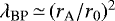 , where rA is the cylindrical radius at the Alfvén surface (where the gas poloidal velocity is equal to the poloidal Alvénic velocity
 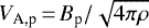 with Bp the poloidal field intensity and ρ the volume density). The Alfvén surface is illustrated in Fig. 1 for our reference self-similar solution.
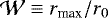
The second emerging property, affecting both the wind geometry and rotation speed, is the wind widening factor  which we define as
 (4)
(4)
where rmax is the maximum radius reached by the streamline launched from radius r0 in the disk before it starts to (slowly) recollimate towards the axis. The value of  is found by solving self-consistently for the transverse force balance between wind magnetic surfaces (see discussion in Ferreira 1997). This parameter is illustrated in Fig. 1 for our reference solution.
For easy reference, our four computed solutions are denoted in the following as LxWy with x = λBP and y =  , and are summarized in Table 1.
- 1.
L13W36, with λBP = 13.7 and
 , is the solution showing the best fit to tentative rotation signatures across the base of the DG Tau atomic jet (Pesenti et al. 2004); it was used by Panoglou et al. (2012) to demonstrate the molecule survival in a dusty disk wind, and by Yvart et al. (2016) to fit H2O line profiles observed by Herschel towards embedded protostars.
 - 2.
L13W130 with λBP = 12.9 and
 is a new solution with a much larger widening.
 - 3.
L5W30 is a new, slower solution with λBP = 5.5 and a widening factor
 comparable to L13W36.
 - 4.
L5W17 is another new, slow solution with λBP = 5.5 and an even smaller widening
 . This solution is our reference model in the following sections, and its geometry is illustrated in Fig. 1.
The input physical parameters of the disk and the heating function at the disk surface used to obtain our solutions are given in Appendix A, together with the calculated density and magnetic field distributions along the wind streamlines.
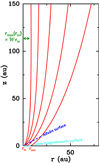 |
Fig. 1 Poloidal cut of a self-similar, axisymmetric MHD DW for our reference solution (L5W17). Selected flow surfaces are plotted in red. Four important model parameters affecting predictedrotational signatures are illustrated here: the inner and outer launching radii, rin and rout, of the wind-emitting region (taken as 0.5 au and 8 au in this graph); the magnetic lever arm parameter λBP (here = 5.5)
|


2.2 Collimation and kinematics of MHD DW solutions
Figure 2 compares the (self-similar) shape and velocity field of the wind streamlines for our four computed MHD DW solutions. Cylindrical coordinates are adopted, and hereafter we use r to denote the cylindrical radius, Vz the velocity component parallel to the jet axis, Vϕ the azimuthal (rotation) velocity, and Vr the radial (sideways expansion) velocity.
Figure 2a shows that the maximum radius is reached further out (i.e., at a larger value of z∕r0) when the widening factor  in increased. After the maximum widening, the streamline slowly bends toward the axis (recollimation zone), until refocussing becomes so strong that the steady-state solution terminates (at z∕r0 ≃ 103−105). This behavior is related to the radial distribution of physical quantities and is a consequence of the dominant hoop-stress in a jet launched from a large radial extent in the disk (see discussion in Ferreira 1997). A recollimation shock may be expected to form beyond this point. However, this region is not reached for the distances to the source and launch radii considered here.
Concerning kinematics, four stages along the propagation of the jet can be distinguished in Figs. 2b–d: below the Alfvén surface, the velocity field is dominated by Keplerian rotation. At the Alfvén surface, the vertical, radial, and toroidal velocities all become comparable (and close to the initial Keplerian velocity at the launch point). Beyond this point, the jet velocity becomes dominated by Vz while Vϕ and then Vr both decrease. Finally, in the recollimation zone where the streamline bends towards the axis, Vr becomes negative and Vϕ increases due to conservation of angular momentum, while Vz keeps its final value.
Figure 2b shows that the increase of Vz along a streamline depends mainly on the magnetic lever arm λBP with little influence of  . The asymptotic value
  is close to the maximum poloidal velocity predicted if all magnetic energy is transferred to the matter (Blandford & Payne 1982):
 (5)
(5)
where VK(r0) is the Keplerian velocity at r0, and the poloidal velocity is defined as  .
.
In contrast, the expansion and rotation velocities depend on both λBP and  , but in different ways. Here, Vr increases with either of these parameters (faster and/or wider flow; cf. Fig. 2d), while Vϕ increases with λBP but decreases for wider solutions (Fig. 2c). This may be understood by noting that, in the “asymptotic regime” (z∕r0 →∞), where the total specific angular momentum L extracted by the wind magnetic torque has been entirely converted into matter rotation, we have
 (6)
(6)
where we use the definition of λBP in Eq. (3). Combining this latter expression with the definition of  in Eq. (4) we find that the minimum Vϕ on a given streamline will scale as
 (7)
(7)
Hence, the minimum rotation velocity reached by a streamline is smaller for wider solutions of the same λBP.
The different dependencies of Vz, Vr, and Vϕ on λBP and  open the possibility to constrain these two parameters from the observed wind spatio-kinematics.
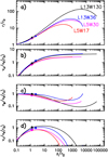 |
Fig. 2 Shape and kinematics of the streamlines as a function of vertical distance z above the disk midplane for the four computed MHD DW solutions in Table 1. a: cylindrical radius r, b: velocity along the jet axis Vz, c: azimuthal rotation velocity Vϕ, d: radial expansion velocity Vr. Filled dots indicate the Alfvén surface. Distances are scaled by the launch radius r0, and velocities by the Keplerian speed at r0, VK (r0). Models are denoted as LxWy with x = λBP the magnetic lever arm parameter and y = |

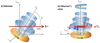 |
Fig. 3 a: definition of inclination angle i for our synthetic predictions in Sect. 3. b: sketch illustrating the construction of the transverse PV cut at projected altitude zcut with a Gaussian beam θb. Wind rotation induces different line-of-sight velocities at symmetric offsets + r and − r on either side of the jet axis, producing a detectable “tilt” in the PV cut (see Fig. 4). This projected velocity shift is used to estimate the rotation speed and specific angular momentum of the flow (see Sect. 3.2). Adapted from Ferreira (2001). |
3 Observed rotation signatures, launch radius, and magnetic lever arm
In an axisymmetric wind, rotation introduces a systematic Doppler shift between spectra from symmetric positions + r and − r on either side of the jet axis; this velocity shift is measured by observers using transverse position–velocity (PV) diagrams built perpendicular to the jet axis, as illustrated in Fig 3.
In Sect. 3.1, we describe the range of free parameters used to compute synthetic transverse PV diagrams for our MHD DW solutions, and our choice of reference case. We then describe in Sect. 3.2 the appearance of PV cuts for radially extended disk winds, and we introduce three methods used by observers to estimate the “observed” specific angular momentum from the PV cuts. Finally, in Sects. 3.3–3.5, we investigate for each method how the launch radius and magnetic lever arm parameter inferred using Anderson’s relations differ from the true rout and λBP of the MHD DW model. Setting robust constraints on these two fundamental parameters is indeed crucial to assess the role of disk winds in disk accretion.
3.1 Free model parameters
As shown in Fig. 2, an MHD DW solution provides us with the self-similar shape of the streamline scaled by the anchor radius r0 of the magnetic surface in the disk, and self-similar velocities scaled by the Keplerian velocity at r0,  . In order to produce synthetic emission predictions comparable to observations, we then need to specify three-dimensional parameters to construct a wind model in physical units (see Fig. 1):
Mass of the central object M⋆: to scale the Keplerian velocity. This parameter has a straightforward influence on line profiles and PV diagrams as it simply stretches the velocity axis by a factor
 . Here we set M⋆ = 0.1 M⊙ as a fiducial Class 0 protostellar mass for consistency with Yvart et al. (2016).
Launch radius rin of the innermost emitting wind streamline: the value of rin depends on the abundance distribution of the observed molecule, which in turn depends on the (poorly known) wind density, irradiation, and temperature. In order to limit the explored parameter space, we keep rin constant in this section. Because the survival of molecules in MHD DWs has been theoretically demonstrated so far only on dusty streamlines (Panoglou et al. 2012; Yvart et al. 2016), we set rin in our models to a fiducial value of 0.25 au, the typical dust sublimation radius in solar-mass protostars. The resulting maximum poloidal velocity is 50–90 km s−1 for λBP = 5.5–13 and M⋆ = 0.1 M⊙. For a given radial extent (rout/rin), a change in rin would simply stretch the velocity axis by a factor
 without changing the PV shape.
Launch radius rout of the outermost emitting wind streamline: this radius, which is one of the key quantities that we wish to determine from observations, is kept as a free parameter. We explored a range of rout = 0.5−32 au corresponding to radial extensions (rout/rin) of 2–130. As a reference case, we arbitrarily choose an intermediate value of rout = 8 au, corresponding to rout/rin = 32.
Once the physical model is constructed (see Fig. 1), we also need to specify four “observational” parameters that affect the synthetic predicted PV diagrams:
Inclination angle i of the jet axis with respect to the line of sight (illustrated in Fig. 3a): we restrict ourselves to inclinations from i = 40° to 90°, which are the most favorable to detect rotation signatures and cover 80% of random orientations. We choose 87° (the inclination of HH212) as our reference model. We show only the red lobe. Position–velocity diagrams for the blue lobe can be easily recovered by the operation Vproj →−Vproj and r →−r.
-
Power-law index α of the line emissivity decline with radius: in principle, knowledge of the emissivity function requires full thermo-chemical and nonlocal thermodynamic equilibrium (NLTE) line excitation calculations, as done by Yvart et al. (2016) for H2O line predictions. In this work, since we aim to present general synthetic observations for a much broader range of MHD DW solutions, a parametrized emissivity function is adopted with a simple power-law radial variation4 :
 (8)
(8)We choose α = −2 as a reference value (based on our modeling of ALMA observations of HH212 in Tabone et al. 2017, and Sect. 4). We also explored α = 0, −1, −3 in our reference model.
Spectral and spatial resolutions: A fiducial 0.44 km s−1 spectral sampling is adopted, typical of what is routinely achieved with interferometric observations of faint lines. Synthetic channel maps are then convolved by a Gaussian spatial beam with a FWHM θb. We choose θb = 225 au as reference, corresponding to a 0.5′′ beam for a source in the Orion molecular cloud (at ≃450 pc). We also explored θb = 45−380 au.
Position zcut where the transverse PV diagram is built: In the context of rotating disk winds from young protostars, contamination by the rotating infalling envelope close to the source (not modeled here) has to be minimized. At the same time, observations must be made sufficiently close to the source to probe a suspected pristine stationary MHD DW minimally affected by shocks or variability (Tabone et al. 2018). A typical distance corresponding to one beam thus appears as a natural choice for zcut. Considering the adopted fiducial beam, we set zcut = θb = 225 au for the reference case. We also explore the effect of a smaller zcut = 70 au in the reference case at i = 87°.
In summary, as a reference model, we choose the L5W17 MHD DW solution (λBP = 5.5,  = 17) with M⋆ = 0.1 M⊙, rin = 0.25 au, rout = 8 au, i = 87°, α = −2, and θb = 225 au, and perform a PV cut across the redshifted lobe at zcut = 225 au. At this distance from the source, z∕rout = 28 and the outermost radius of thejet has thus reached rj ≃ 10 rout ≃ 80 au (see Fig. 2a). In the following, we vary each of the above free parameters except for M⋆ and rin (which only set the velocity scale), to see how they impact apparent rotation signatures, and the launch radius and magnetic lever arm inferred from them using Anderson’s relation.
3.2 Methods for measuring rotation from transverse PV cuts
Let us first consider the simple case where only a narrow rotating ring of wind material emits in the selected line tracer. The transverse PV cut then resembles a tilted ellipse, whose major and minor axes and tilt angle are given in Appendix B.1 as a function of the flow velocity field.
Let us also assume that the ring is better resolved spectrally than spatially, as is usually the case in ALMA-like observations. The PV ellipse then presents two emission peaks symmetrically positioned at (see Appendix B.2)
 (9)
(9)
and
 (10)
(10)
where
 (11)
(11)
is the transverse velocity modulus (in the plane perpendicular to the jet axis), rj the flow radius, and Vz, Vϕ, Vr are the vertical, azimuthal, and radial expansion speeds, all measured at z = zcut on the outermost emitting streamline launched from rout.
The spatial and velocity separations between the two PV peaks, Δrth and ΔVth, are then given by:
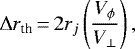 (12)
(12)
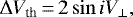 (13)
(13)
and the true specific angular momentum on the outer streamline, jout, is given by
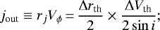 (14)
(14)
we note that V⊥ cancels out in the product of Δrth and ΔVth.
However, a narrow range of streamlines is not the most probable case if the MHD DW dominates the extraction of angular momentum from a sizable portion of the disk, and the chosen tracer is not too chemically selective (e.g., CO, SO).
When the wind streamlines span a broad range of radii and Vz, we find that PV cuts are no longer elliptical and that two broad configurations exist, with a transition around a critical inclination angle icrit ≃ arctan(∣ Vz ∣ ∕V⊥) (≃ 84° for our models, see Table 1). At large inclinations, i > icrit, which we denote “edge-on” in the following for brevity, PV cuts remain double-peaked regardless of model parameters, with peaks of opposite velocity sign. This phenomenon is illustrated in Fig. 4a for our reference MHD DW model at i = 87°.
In contrast, at moderate inclinations i < icrit, PV cuts become more complex, with curved emission ridges that stretch over a wide velocity interval. One or two main peaks may result; these rapidly shift or merge along the ridges with small changes in the parameters (spatial beam, emissivity gradient α, wind radial extension, etc.). An example is shown in Fig. 4b for our reference model at i = 70° with α = 0: the PV cut is double-peaked for θb = 45 au but becomes single-peaked for θb = 225 au. In this configuration, the PV double-peaks (of the same velocity sign when present) cannot be used as reliable rotation estimators.
In the following, we therefore consider three methods used by observers to estimate the flow specific angular momentum from PV cuts at ALMA-like resolution. These are briefly described in turn below. The resulting biases in launch radius and magnetic lever arm are discussed in Sects. 3.3–3.5.
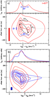 |
Fig. 4 a: on-axis spectrum and transverse PV diagram for the reference model viewed at i = 87°, illustratingthe “edge-on” case. The two red dots indicate the intensity peaks in the PV, which have opposite velocity signs in this configuration; their connecting line defines the spatial and velocity separations Δr and ΔV used to estimate the observed specific angular momentum jobs in Eq. (15). We also plot in black the ellipse and peak positions contributed by the outermost streamline alone, which predict a similar velocity shift ΔVth (see Eq. (13)) but a much larger spatial shift Δrth (see Eq. (12)). Other model parameters are: zcut = 225 au, M* = 0.1 M⊙, rin = 0.25 au, rout = 8 au, α = − 2, and θb = 225 au. Filled rectangles show the spectral and angular resolutions. b: same as (a) but at lower inclination i = 70° (note the change in velocity scale) for α = 0 and θb = 225 au (red) and 45 au (blue). Double-peaks in the PV diagram now have the same velocity sign, and can vanish at moderate angular resolution. |
3.2.1 Double-peak separation method
For a double-peaked transverse PV, it is easiest, and customary in observational studies in the literature, to estimate the specific angular momentum carried by the flow by analogy with the single annulus case (Eq. (14)) as (e.g., Zapata et al. 2015; Chen et al. 2016; Lee et al. 2018a; Zhang et al. 2018),
 (15)
(15)
where ΔV is the observed velocity shift between the two intensity peaks in the PV cut, and Δr is their spatial centroid separation perpendicular to the jet axis (see blue arrows in Fig. 4a).
In Sect. 3.3, we extensively investigate the double-peaked method for edge-on inclinations (i ≥ icrit), where the peaks have opposite velocity signs. We show that the result is remarkably independent of beam size, and leads to systematic underestimation of jout, rout, and λBP (Sects. 3.3.1–3.3.3).
In contrast, at lower inclinations where PV double peaks have the same velocity sign (i < icrit), this method cannot yield robust results – and is not recommended. The existence and positions of double peaks are too sensitive to the exact combination of parameters (see discussion of Fig. 4b above), and would also be very sensitive to noise fluctuations along the underlying ridges. We therefore only consider the following two methods in that case.
3.2.2 Rotation curve method
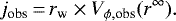
Following optical jet rotation studies with HST (Bacciotti et al. 2002; Coffey et al. 2007), a more generic method applicable to all inclinations and PV morphologies consists in deriving an “observed” rotation curve Vϕ,obs(r) from velocity shifts between symmetric spectra at ± r from the jet axis, through
![Mathematical equation: \begin{equation*}V_{\phi,\rm obs}(r)\,{=}\,\left[ V(r)-V(-r) \right] / 2\sin{i}, \end{equation*}](/articles/aa/full_html/2020/08/aa34377-18/aa34377-18-eq37.png) (16)
(16)
from which the local specific angular momentum on each flow surface of radius r may be estimated as (Anderson et al. 2003)
 (17)
(17)
This more elaborate method has only recently started to be applied to ALMA data (e.g., Bjerkeli et al. 2016). We illustrate the typical observational bias associated with this method in Sect. 3.4, and show that it leads to overestimation of rout in our models, except when the flow is adequately transversally resolved.
3.2.3 Flow width method
Another generic but more simple method, which is mainly used when the flow is not well resolved transversally, is to take (e.g., Lee et al. 2008)
 (18)
(18)
where Vϕ,obs(r∞) is the asymptotic value of the rotation curve at large radii (assumed to trace the true rotation speed on the outer streamline) and rw is the deconvolved flow radius estimated from emission maps (assumed to trace the true outer flow radius rj). In Sect. 3.5, we show that in our models, this method systematically underestimates rout and λBP (by a similar amount as the double-peaked method in edge-on flows).
3.3 Double-peak separation: biases in edge-on flows
As explained in the previous section, we restrict our investigation of this method to quasi edge-on inclinations where the PV cut has double peaks of opposite sign. We note that this edge-on configuration maximizes the chances of detecting rotation shifts (∝ sin i) and minimizes contaminating shifts caused by slight asymmetries in poloidal velocity (∝ ΔVp cosi).
We study this method in particular detail as it was used recently to measure rotation speeds in the edge-on SO outflow in HH212 (Lee et al. 2018a). This prototypical object was studied with ALMA over a remarkably wide range of angular resolutions (factor 15), and allows us to carry out several stringent tests of our predictions (see Sect. 4).
3.3.1 Bias in angular momentum
The outermost DW launch radius rout is the most critical parameter. Observers seek to estimate this latter in order to discriminate among disk accretion paradigms (see Sect. 1). We therefore compare the apparent specific angular momentum jobs, measured from the double-peak spatial and velocity separations Δr and ΔV (using Eq. (15)), with the true specific angular momentum jout along the outermost emitting DW streamline.
As a first example, we consider our reference model shown in Fig. 4a. The black ellipse and black dots show the predicted ellipse and emission peaks for a single ring on the outermost streamline. It may be seen that the observed velocity separation of PV peaks, ΔV, agrees with the predicted velocity separation ΔVth. In contrast, the spatial separation Δr is smaller than the predicted spatial separation Δrth by roughly a factor three. As a result, the value of jobs inferred from the double peak separation with Eq. (15) underestimates the true jout (see Eq. (14)) also by a factor three, which is quite significant.
To show that this bias is generic to the method, and how it depends on each free parameter, we compare in Fig. 5 the measured Δr, ΔV, jobs on PV cuts to the true values of Δrth, ΔVth, jout for a series of edge-on PV models that differ from the reference case by only one free parameter at a time. In addition, the detailed effect of parameter changes on the shape of on-axis spectra and PV diagrams is illustrated in Fig. 6 for selected pairs of models.
Based on Fig. 5 we find that jobs always underestimates jout, and that this systematic bias is essentially due to the peak spatial separation Δr being always much smaller than the predicted value Δrth for the outermost streamline. In contrast, the velocity separation ΔV always remains close to the predicted ΔVth (except when i approaches icrit, where ΔV drops).
A striking result is that this bias does not improve at higher spatial resolution (Fig. 5d). It does not vary much either with position of the PV cut (Fig. 5d), or magnetic lever arm and widening of the MHD solution (Fig. 5a). In contrast, increasingly severe underestimation occurs with increasing radial extension rout∕rin of the MHD DW (Fig. 5b), and with the slope of the radial emissivity gradient, controlled by the power-law index α (Fig. 5c).
From this behavior, we conclude that the underestimation of Δr is a contrast effect attributable to the contribution of bright nested streamlines interior to rout, projected at low-velocity by the quasi edge-on inclination. As an example, the two spectra in Fig. 6b show that, at the velocities of the PV peaks, inner streamlines launched within r0 ≤ 1 au (blue curve) contribute about 30% of the total line intensity integrated up to rout = 8 au (red curve). This contribution of inner streamlines drags the spatial centroids of the PV peaks closer to the axis than if emission came only from a narrow ring on the outermost streamline. The peak spatial separation Δr is thus reduced compared to the theoretical value Δrth. When the radial extension of the MHD DW grows, or when the radial gradient of emissivity steepens, the relative flux contribution of inner versus outer streamlines automatically increases and the reduction in Δr is more severe, reaching up to a factor of between three and ten in Figs. 5b and c. An even larger bias would be created if both effects (a large radial extension ≃100 and a steep emissivity gradient α = −3) conspired together.
3.3.2 Bias in the outer launch radius, rout
Since errors in jobs in the edge-on configuration do not depend significantly on the specific MHD solution, inclination, beam size, or the position of the PV cut (see Sect. 3.3.1), we focus in the following on our reference edge-on model and vary only the wind radial extension (rout∕rin) from 2 to 130 (with α fixed at −2) or the emissivity index α from 0 to −3 (with rout fixed at 8 au).
Figure 7a shows the absolute value of jobs for this restricted set of models as a function of the radial extension. Figure 7b shows the “observed” poloidal velocity Vp,obs, estimated by deprojecting the average line-of-sight velocity ⟨V ⟩ of the two PV peaks:
 (19)
(19)
We see that Vp,obs provides a good estimate of the true Vp(rout) up to (rout∕rin) ≃ 20, and progressively overestimates it for a more extended wind.
Figure 7c plots the values of launch radii robs obtained by solving Anderson’s relation in Eq. (1) with rVϕ = jobs, V ≃ Vp,obs (Vϕ is negligible here), and R ≫ r0 (largely fulfilled at zcut = 225 au).
As one might have expected, we find that robs takes a value intermediate between rin and rout. It therefore only gives a strict lower limit to the true outermost launching radius of the emitting disk wind. In addition, this bias becomes greater with increasing MHD DW radial extension. In our reference model, the error reaches a factor ten for rout = 32 au, which is a very significant effect.
Figure 7c also shows that for our reference emissivity index α = −2, robs grows roughly as the geometrical average of the innermost and outermost launch radii. One might then think of recovering the true rout value as
 (20)
(20)
However, the geometrical average only holds when α = −2. For a steeper emissivity gradient (α = −3), robs is closer to rin, while for a shallower gradient (α = −1, 0), robs is closer to rout (see green dots in Fig. 7c). Since Eq. (20) is quadratic in robs, an α value differing from −2 could introduce a large errorin rcorr (factor 4–9at rout = 8 au, cf. green dots Fig. 7c). Another problem is encountered when choosing the relevant value of rin to use in Eq. (20). Although we fixed this latter parameter for simplicity at the dust sublimation radius ≃ 0.25 au in this section, rin in actual disk winds will depend on the chosen chemical tracer and wind density: it could move well outside to ≥ 1 au in evolved disk winds where FUV photodissociation is important (Panoglou et al. 2012; Yvart et al. 2016) or well inside to rin ≃ 0.05–0.1 au if inner streamlines are dense enough for efficient dust-poor chemistry (Tabone et al. 2020), as recently suggested in the dense Class 0 flow of HH212 by model fits to PV cuts (Tabone et al. 2017). This introduces an additional uncertainty of a factor four either way in Eq. (20).
We conclude that when the MHD DW is radially extended and viewed close to edge-on (i.e., with PV double peaks of opposite signs), the launch radius robs inferred from the double-peak separation using Anderson’s relation only gives a lower limit to the true rout. This bias cannot be accurately corrected for without additional constraints on rin and the radial emissivity gradient (α).
 |
Fig. 5 Double-peak separation in edge-on PVs of radially extended DWs (connected dots) compared with the theoretical value for a single wind annulus on the outermost streamline (dotted curves). Left column: observed spatial separation Δr vs. theoretical Δrth (from Eq. (12)); middle column: deprojected velocity shift ΔV ∕sin i vs. theoretical value ΔVth∕sin i (from Eq. (13)). Right column: ratio of the apparent specific angular momentum jobs = (Δr∕2) × (ΔV∕2sin i) to the true value on the outermost streamline, jout = (Δrth ∕2) × (ΔVth∕2sin i). From top to bottom panels: the influence of varying (a) MHD solution (colour-coded) and inclination angle; (b) outermost launching radius rout of the emitting region of the MHD DW; (c) index α of the emissivity radial power law (see Eq. (8)); and (d) spatial beamFWHM θb and PV cut position zcut. All nonlabeled model parameters are fixed at their reference value: i = 87°, MHD solution = L5W17, rout = 8 au, α = − 2, θb = 225 au, zcut = 225 au, M⋆ = 0.1 M⊙, and rin = 0.25 au. Datapoints for this reference case are circled in orange in each panel. |
 |
Fig. 6 Comparisons of synthetic on-axis spectra and transverse PV cuts at zcut = 225 au for selected pairs of quasi edge-on models that differ by only one parameter at a time. In red, we show the reference model with i = 87°, rout = 8 au, α = − 2 (see Eq. (8)), θb = 225 au, λBP = 5.5, and |

3.3.3 Bias in magnetic lever arm
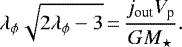
Figure 7d plots the “observed” wind magnetic lever arm parameter λobs inferred from the values of jobs and robs in Figs. 7a and c following Anderson’s method (see e.g., Anderson et al. 2003):
 (21)
(21)
For comparison, we also plot (dotted curve) λϕ (rout), the equivalent physical quantity on the outermost streamline that would be obtained in the case of no observational bias (i.e., for a single emitting ring):
 (22)
(22)
Figure 7d shows that λobs gives a strict lower limit to λϕ (rout); however, this observational bias is very mild (−20% for α = −2 and a factor two for α = −3) and is independent of the wind radial extension.
This fortunate result is not a coincidence: expressing rVϕ as  in Anderson’s relation of Eq. (1), we see that once gravitational potential has become negligible (R ≫ r0), the total velocity modulus must verify5
 (23)
(23)
Noting that our models have V ≃ Vp at large distance, we obtain the following useful relation, where launch radius cancels out (see Eq. (10) in Ferreira et al. 2006):
 (24)
(24)
For r0 = robs Anderson’s relation imposes the same relation between λobs, jobs, and Vp,obs. For moderate magnetic lever arms, λ ≲ 6, such as those considered here, the function on the left-hand side of Eq. (24) is very steep; hence even if jobs is smaller than jout by a large factor (Fig. 7a), the bias in the inferred λobs is much smaller (Fig. 7d).
We also observe a theoretical “MHD bias” in that λϕ (rout) is always smaller than the true λBP in the solution. As first pointed out by Ferreira et al. (2006), this bias arises because λϕ only measures the specific angular momentum in the form of matter rotation, whereas the total (conserved) specific angular momentum L carried by the MHD DW streamline (and measured by λBP) also includes a contribution of magnetic field torsion. The dotted curve in Fig. 7d (constructed at zcut = 225 au) shows that in our reference solution, λϕ(r0) reaches 90% of λBP when z∕r0 = 550, 70% when z∕r0 ≃ 20, and only 50% when z∕r0 ≃ 7.
In conclusion, we find that the magnetic lever arm parameter inferred with Anderson’s method only gives a lower limit to the true λBP. This is mainly caused by an MHD bias (hidden angular momentum in magnetic form), with only a minor observational bias for low λBP. Here, λBP can only be accurately estimated at high altitudes (zcut ≥ 20rout for our self-similar models), or by modeling the whole PV cut in detail with a self-consistent MHD DW solution (see e.g., Sect. 4 for the example of HH212).
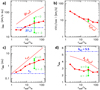 |
Fig. 7 Observational biases in the PV double-peak separation method for our reference edge-on case (i = 87°), as a functionof the DW radial extension (for α = −2, connected red dots) and emissivity index α (for rout/rin = 32, connected green dots): panels a and b show specific angular momentum and poloidal velocity estimated from the PV double-peak separation; c and d show launch radius and magnetic lever arm parameter inferred from the observed quantities in (a) and (b) using Anderson’s relations (Eqs. (1) and (2)). Values that would be obtained for a single ring on the outermost wind streamline are shown in dotted red curves. The true magnetic lever arm parameter λBP of the MHD solution and relevant values at rin are indicated for reference in dot-dashed blue. |
3.4 Rotation curve method: biases in launch radius and magnetic lever arm
For consistency, we consider the same reference MHD DW parameters and zcut = 225 au as in the previous section. We find that at moderate inclinations, i < icrit, the observed rotation curves from velocity shifts (Eq. (16)) depend strongly on whether the wind is transversally resolved or unresolved. We present in Fig. 8a the curves for i = 40° to 80° with θb = 45 au < rj illustrating the well-resolved regime, and in Fig. 8b the curves with θb = 225 au > rj illustrating the unresolved regime. Results for more edge-on inclinations, which are independent of beam size, are discussed at the end of this section.
Figure 8a shows that in the well-resolved flow regime, Vϕ,obs(r) follows the underlying true rotation curve Vϕ(r) within a factor two, until r ≤ θb∕2, where it falls sharply below the curve due to beam smearing. In contrast, Fig. 8b shows that in the unresolved regime, Vϕ,obs(r) does not follow the Keplerian decline but instead increases slowly with radius. At large radii, where emission has dropped to 10% of the PV peak, Vϕ,obs(r) reaches about 60–80% of the true rotation speed on the outermost streamline.
We note that rotation curves in Fig. 8 exhibit little change with inclination, except when i = 80° where they flatten out to become almost independent of radius, as we approach icrit (≃ 84° for the L5W17 reference solution). Similar results were found for rout = 8 au and 32 au. In the following, we therefore take i = 40° and rout = 8 au (red curves in Fig. 8) as our representative model for moderate inclinations. In Fig. 9a, we plot for this representative model the DW launch radii robs(r) inferred by applying Anderson’s formula to the observed local specific angular momentum at each r:
 (25)
(25)
using the corresponding observed local poloidal velocity,
![Mathematical equation: \begin{equation*} V_{\textrm{p, obs}}(r)\,{=}\,\left[ V(r)+V(-r) \right] / 2\cos{i}.\end{equation*}](/articles/aa/full_html/2020/08/aa34377-18/aa34377-18-eq48.png) (26)
(26)
Similarly, in Fig. 9b, we plot as a function of r the magnetic lever arm parameters λobs(r) inferred from robs(r) and jobs(r) using Eq. (21).
In the spatially resolved regime (green curves), the method performs very well, with little observational bias. In particular, the results at 10% intensity level give relatively accurate values of rout and of λϕ (rout) (defined in Eq. (22)).
In the unresolved regime (red curves), robs(r) and λobs(r) suffer complex observational biases: They take artificially small values at radii r ≤ rj (where rotation speeds are strongly underestimated by beam smearing) and overshoot the true rout and λϕ (rout) at large radii. This overshoot is caused by the beam smearing artificially enlarging r well beyond the true rj, so that jobs(r) at 10% intensity level exceeds jout. This bias will of course become greater with increasing (θb∕rj), and providesupper limits to the true rout and λϕ (rout).
Finally,we discuss the rotation curve method in the quasi edge-on case: As shown by outer contours of PV cuts in Fig. 6, velocity shifts between ± r in that case are approximately constant with radius and close to ΔV, the velocity separation between the PV double peaks. The latter was found to be close to ΔVth (see Eq. (13) and Fig. 5). It follows that the (constant) value of Vϕ,obs(r) will be close to  , i.e., slightly larger than Vϕ on the outer streamline. The inferred jobs at 10% intensity radius (where r ≥ rj) will thus again overestimatethe true jout (by an amount that depends on beam smearing) and provides upper limits to rout and λϕ (rout).
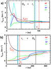 |
Fig. 8 “Observed” rotation curve Vϕ,obs(r) obtained from the difference of peak velocity between ± r from the jet axis (Eq. (16)) for our reference model viewed at i = 40°, 60°, 70°, and 80° (color-coded curves). (a): Spatially resolved regime (θb = 45 au), (b): spatially unresolved regime (θb = 225 au; we note the change of scales on both axes). In both panels, a vertical black line indicates the beam FWHM, and colored vertical dashed lines indicate the flow radius rj at zcut = 225 au. The true wind rotation curve Vϕ(r) at z = zcut∕sin i) is shown by dotted curves, with a constant value beyond rj. The cross on the red curve illustrates where the local intensity drops below 10% of the PV peak. |
3.5 “Flow width” method: biases in launch radius and magnetic lever arm
Here, jobs is obtained from the asymptotic rotation speed at large radii and the deconvolved flow radius as
 (27)
(27)
To estimate rw, observers typically measure the FWHM of the beam-convolved velocity-integrated map at zcut and correct in quadrature for the Gaussian beam broadening to yield an intrinsic wind FWHM, which is then assumed equal to the wind diameter so that:
 (28)
(28)
We performed this measurement on the synthetic integrated emission maps for our reference model at i = 40°. With θb = 225 au, we find rw = 27 au, a factor four smaller thanthe true outer flow radius rj at that position. With a smaller θb, for example θb = 45 au, which fully resolves the flow transversally, rw is almost unchanged at 20 au. Therefore, rw ≪ rj is not a beam smearing effect; it occurs because the FWHM in emission maps is dominated by the central spine of inner bright streamlines, and does not encompass the fainter pedestal tracing the outermost streamlines. The wind therefore appears much narrower than it really is (“optical illusion” effect). It is significant that the deconvolved flow diameter 2rw is of the same order as the double-peak spatial separation Δr for the same model viewed at i = 87° (see Fig. 5), and that both are independent of beam size. Indeed, their strong reduction compared to the true flow width has the same root cause, namely the brightness contrast between inner and outer streamlines.
Figure 8 shows that the asymptotic rotation velocity at 10% intensity level, Vϕ,obs(r∞) ≃ 0.8−1 km s−1, is also not strongly affected by beam smearing; it is also relatively unaffected by inclination, and is close to the true rotation speed on the outer streamline. Using Eq. (27), we obtain with the flow width method jobs ≃ 20–22 au km s−1 for θb = 45–225 au. Combining with the observed Vp,obs ≃ 7–8 km s−1 at 10% intensity, and applying Anderson’s relations, we infer robs ≃ 1.5 au and λobs ≃ 2. These values are slightly smaller but very close to what we obtained with the double-peaked method in the same model viewed edge-on (see Fig. 7 with rout/rin = 32). This is not surprising, since we see that rw is close to Δr∕2 while Vϕ,obs(r∞) is close to Vϕ, which is itself only slightly smaller than  (see Fig. 5 and associated discussion in Sect. 3.3.1).
We conclude that the “flow width” method will lead to underestimate jout by a similar amount to the double-peak separation method in the same flow viewed edge-on, and will yield strict lower limits to the true rout and λBP.
 |
Fig. 9 Examples of bias when using the rotation curve method for a representative model at i = 40° (in red in Fig. 8): “Observed” launch radii robs(r) (a) and magnetic lever arms λobs(r) (b) inferred at each r by application of Anderson’s formula to jobs(r) and Vp,obs(r) (Eqs. (25) and (26)). Green curves illustrate the spatially resolved regime (θb = 45 au) and red curves the unresolved regime (θb = 225 au). These curves stop at 1% of the PV peak intensity, with a plus symbol marking 10%. The black vertical line shows the flow radius rj. For comparison, dotted blue curves plot the true launch radii r0(r) (a) and λϕ(r) (b) of each DW streamline tangent to r; horizontal dashed blue lines mark the true outermost launch radius rout = 8 au (a) and true λBP = 5.5 (b) in the model. Other model parameters are: MHD solution L5W17, α = −2, M⋆ = 0.1 M⊙, and rin = 0.25 au. |
4 Application to the edge-on rotating flow in HH212
The edge-on flow HH212 (viewed at i = 87°) exhibits a slow and wide rotating SO outflow first identified by Tabone et al. (2017) as a possible MHD disk wind candidate. In this section, we use three sets of ALMA observations of HH212 spanning a factor 15 in angular resolution to verify our main results on the double-peak separation in edge-on PV cuts (Sect. 3.3) and to test the DW model of Tabone et al. (2017) down to ≃ 18 au resolution (Lee et al. 2018a). We also derive an analytical formula for the fraction of disk angular momentum extracted by a self-similar MHD DW, and apply it to HH212.
For consistency with our previous modeling work of HH212 in Tabone et al. (2017), we adopt a systemic velocity of Vsys = 1.7 km s−1 (Lee et al. 2014)and a distance d = 450 pc. Recent VLBI parallax measurements towards stellar members of the Orion B complex yield mean distances of 388 ± 10 pc for NGC 2068 and 423 ± 15 pc for NGC 2024 (Kounkel et al. 2017), suggesting a possibly closer distance to HH212 of ≃ 400 pc, located in projection between these latter two regions. However, the exact distance to HH212 remains uncertain; adopting 400 pc instead of 450 pc would decrease linear dimensions and mass-outflow rates by 10%, and the mass-accretion rate by 20%, without altering our conclusions.
4.1 Effect of angular resolution on apparent rotation signatures in HH212
Here, we first use HH212 to verify our most counter-intuitive theoretical prediction for a quasi edge-on MHD DW, namely that the spatial shift Δr between the redshifted and blueshifted PV emission peaks does not depend on beam size (see Sect. 3.3.1).
Figure 10 shows SO maps of blueshifted and redshifted emission of the base of the HH212 flow obtained at 0.55″ ≃ 250 au resolution in ALMA Cycle 0 by Podio et al. (2015). The maps are integrated over the intermediate velocity range 1.5 km s−1 < ∣VLSR − Vsys∣ < 2.8 km s−1, where Tabone et al. (2017) found a clear transverse spatial shift between the blueshifted and redshifted emissions at higher resolution of 0.15″ ≃ 65 au (see their Fig. 2b). Although no obvious shift between blue and red contours is apparent at first sight in Fig. 10, the signal-to-noise ratio (S/N) of these data is high enough for spatial shifts much smaller than the beam to still be detected by comparing centroid positions (the so-called “spectro-astrometry” technique). At each distance z along the jet axis, a transverse intensity cut is constructed across the blue and the red channel maps and the spatial centroid measured in each cut. These centroids are plotted in Fig. 10 as blue and red dots, respectively. A small but significant and consistent transverse position shift between redshifted and blueshifted emission centroids is clearly detected; it persists out to z±0.7′′. The shift amplitude at z ≃ 70 au is Δr ≃ 0.06″ ± 0.02″ (27 au), in the sense of disk rotation. The same shift is measured with this method in the higher resolution 0.′′ 15 data of Tabone et al. (2017). Since the channel maps are separated by ΔV = 4 km s−1, the apparent specific angular momentum in both data sets is jobs = (Δr∕2)(ΔV∕2) ≃ 27 au km s−1.
The apparent specific angular momentum in the SO wind of HH212 was measured at yet higher angular resolution (0.′′ 04) by Lee et al. (2018a). Their value of ≃ 30 ± 15 au km s−1 remains remarkably similar to our results at 0.′′55 and 0.′′ 15. We therefore verified, from more than a decade in beam sizes, that the apparent specific angular momentum measured from the separation between blue and red PV peaks in a quasi edge-on flow does not depend on angular resolution, as predicted for an MHD DW (see Fig. 5d).
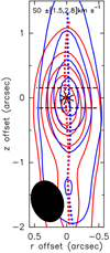 |
Fig. 10 Rotation signatures retrieved at 225 au resolution by spectro-astrometry towards the low-velocity HH212 outflow. Blue (resp. red) contours show SO(98−87) blueshifted (resp. redshifted) emission over intermediate velocities (1.5 km s−1 < ∣ VLSR − Vsys∣ < 2.8 km s−1) mapped with ALMA Cycle 0 (from Podio et al. 2015). The blue (resp. red) dots mark the centroid positions of transverse intensity cuts at each altitude across the blue (resp. red) contour maps. The black asterisk indicates the continuum peak. The jet was rotated to point upwards for clarity. Horizontal black dashed lines depict the position of PV cuts at z ± 70 au shown in Fig. 11. The clean beam FWHM of 0.65″ × 0.47″ is shown as afilled black ellipse. First contours are 0.1 mJy beam−1 km s−1 and steps are 0.15 mJy beam−1 km s−1. |
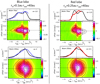 |
Fig. 11 Comparison between observed and modeled SO on-axis spectra and transverse position-velocity cuts taken at ± 0.′′15 (70 au) across the blueshifted (left panels) and redshifted (right panels) lobes of the HH212 jet. Top row: ALMA Cycle 4 data (70 au beam) from Tabone et al. (2017). Bottom row: ALMA Cycle 0 data (250 au beam) from Podio et al. (2015). In all panels, observed spectra are plotted as histograms, and observed PV diagrams are shown as color maps with white contours. Synthetic predictions for the MHD DW model of Tabone et al. (2017), convolved by the appropriate beam size, are overplotted in black. The model uses the MHD DW solution L5W30, M⋆ = 0.2 M⊙, i = 87°, with the range of launch radii (rin, rout) indicated on top. The best-fitting emissivity variation index (α) is marked ineach panel. |
4.2 Best-fitting rout and MHD DW model versus angular resolution
Using the apparent specific angular momentum ≃30 au km s−1 determined above, a mean deprojected poloidal speed of Vp,obs ≃ 1 km s−1 ∕ cosi ≃ 20 km s−1, and M⋆ = 0.2 M⊙, Anderson’s relation yields an estimated robs ≃ 1 au.
We show below that the true outer launch radius rout of the HH212 SO wind is actually much larger than this, and is close to the disk outer radius of 40 au in HH212, confirming our predicted bias that robs ≪ rout with the double-peak separation method (see Sect. 3.3.2). We also show that the MHD DW model with rout = 40 au initially proposed by Tabone et al. (2017) remains consistent with PV cuts obtained at both four times lower and higher resolution.
In Fig. 11, we compare on-axis spectra and transverse PV diagrams of SO at the same zcut = ±70 au for a resolution of ≃ 70 au (Tabone et al. 2017) and a four times larger beam ≃250 au (Podio et al. 2015); we note that we were not able to perform the same comparison in the SO2 line, where the S/N in Cycle 0 was too low). The MHD DW model proposed by Tabone et al. (2017), convolved by the appropriate clean beam in each case, is superimposed in back contours. This latter model was obtained with the MHD DW solution L5W30, rout = 40 au, M⋆ = 0.2 M⊙, i = 87°, and rin = 0.1 au (blue lobe) or 0.25 au (red lobe).
Figure 11 shows that the same model can also reproduce the SO PV cut at a four times lower angular resolution reasonably well, with just a slight change in radial emissivity gradient6 (α = −2 (blue lobe) or −2.5 (red lobe), instead of −1.8).
In particular, the MHD DW model naturally explains (i) the smaller peak velocity separation at lower angular resolution (cf. the drop of ΔV with beam size at zcut = 70 au visible in the green curves of Fig. 5d); and (ii) the more symmetric profile wings at lower resolution (in the model, this is caused by the larger beam encompassing emission from closer to the disk surface and from the opposite lobe). In conclusion, observationsat 70 and 250 au resolution appear consistent with the same MHD DW model, and in particular the same large rout value.
However, the agreement is not perfect when taking into account the finer details. Towards the red lobe, both datasets in Fig. 11 have their peak emission at redshifted velocities, while the models present a bluer peak. This is due to a global asymmetry in the HH212 SO outflow, in the sense that redshifted emission is systematically stronger than blueshifted emission in both lobes (see e.g., PV cut along the flow in Fig. 5 of Lee et al. 2018a). Such behavior cannot be reproduced by an axisymmetric model like ours, where the brighter peak will necessarily switch sign between the two lobes; it could be explained by an ad-hoc nonaxisymmetric emissivity distribution. When comparing with the 250 au resolution data, we also note that the MHD DW model tends to predict peak velocities that are slightly too large further than 0.2″ from the axis. This outer region might be associated with the limits of the self-similar model assumption due to boundary effects, as discussed in Tabone et al. (2017). Alternatively, recent observations of complex organic molecules indicate temperatures ≃ 150 K near the disk outer edge (Lee et al. 2017b; Bianchi et al. 2017; Codella et al. 2018), suggesting a sound speed in the disk atmosphere reaching 30% of the Keplerian speed at 40 au; therefore, “hot” magneto-thermal DW solutions with a higher mass-loading and smaller magnetic lever arm and rotation speeds (Casse & Ferreira 2000b; Bai & Stone 2013; Béthune et al. 2017) might be more appropriate in these outermost wind regions. Modeling such complex effects lies beyond the scope of the present paper and will be the subject of future work.
In Fig. 12, we turn to smaller scales and compare the MHD DW model of Tabone et al. (2017) with transverse PV cuts obtained by Lee et al. (2018a) in the same SO line7 through the disk atmosphere at z ≤ 45 au, with an unprecedented resolution of0.′′04 = 18 au. A particularly noteworthy aspect is the global velocity shift observed between the two faces of the disk: Indeed, the Keplerian-like patterns fitted by Lee et al. (2018a) at z ≃ ±20 au (pink curves in Fig. 12) are not centered on the systemic velocity but are shifted globally by ≃ −0.3 km s−1 to the blue inthe north (blue) lobe, and by + 0.3 km s−1 to the red in the south (red) lobe. This velocity shift implies that rotating disk layers probed by SO are not static but outflowing all the way out to rout ≃ 0.1″ ≃ 45 au, with a mean deprojected vertical velocity on each side Vz ≃ 0.3∕cos(87°) ≃ 6 km s−1. This observation directly confirms, independently of any model, that the launch radius inferred with Anderson’s relation from the PV double-peak separation (robs ≃ 1 au, see above) severely underestimates the true disk wind radial extent.
Figure 12 further shows that the MHD DW model proposed by Tabone et al. (2017) naturally reproduces not only theglobal velocity shift between the two faces of the disk, but also the overall envelope of the emission in the PV cuts at 18 au resolution. The predicted regions of brightest emission (top two contour levels) also generally overlap quite well with the observed ones, although the agreement is again not perfect. The model sometimes extends to slightly higher blue velocities on axis than detected. The exact positions of emission peaks can also differ. However, observed maximum velocities and peak positions are also subject to certain uncertainty due to the moderate signal-to-noise ratio and incomplete u − v coverage at such high angular resolution. Moreover, our MHD DW model is probably too idealized (self-similar,steady, axisymmetric). Given these caveats, and the fact that the model was initially fitted on data at fourtimes lower angular resolution (70 au), we consider the agreement to remain quite promising at this stage.
Nevertheless, our proposed interpretation in terms of MHD DW is not unique. Lee et al. (2018a) proposed an alternative model in terms of a thin, swept-up shell driven by an unseen fast, wide-angle X-wind (see Lee et al. 2001, and green ellipses in Fig. 12). Although this shell has a different velocity field (purely radial motion proportional to distance) from our MHD DW, the large projection effect on Vz at i = 87° makes it difficult to distinguish between them (cf. Fig. 11 in Lee et al. 2018a). A hybrid scenario where an extended disk wind is shocked by inner-jet bow shocks is also conceivable (cf. Tabone et al. 2018). Indeed, wide bow-shock wings are seen in HH212 in SiO at least down to z ≃ 0.′′ 5 ≃ 200 au (Podio et al. 2015; Lee et al. 2017a). Studies of less inclined MHD DW candidates will be crucial to constrain the Vz component and discriminate between these options.
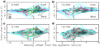 |
Fig. 12 Position–velocity cuts at 0.04′′ ≃ 18 au resolution across the upper disk atmospheres in HH212: black contours and grayscale show SO ALMA observations from Lee et al. (2018a). Cyan contours show synthetic predictions for the MHD DW model of Tabone et al. (2017). zcut is labeled in arcsec in the upper-left corner (>0 in the blue lobe, <0 in the red lobe). Magenta curves in panels a and b plot Keplerian curves fitted by Lee et al. to their data at z ≃ ± 20 au; the blue andred velocity shift of these curves from the systemic velocity suggests an outflow from the disk atmosphere out to rout ≃ 0.1′′≃ 45 au, well reproduced by the MHD DW model; green ellipses in panels a and c show the expanding shell model fitted by Lee et al. in theblue lobe. |
4.3 Role of the HH212 MHD DW candidate in disk accretion
The disk wind streamlines used for our model PV cuts were obtained as part of a global MHD accretion–ejection solution where the wind vertically extracts most of the angular momentum flux required for steady disk accretion (see Appendix A). However, similar emergent disk wind properties could be obtained with a dominant viscous torque in the disk, if the turbulent resistivity is highly nonisotropic (Casse & Ferreira 2000a) or if the disk magnetization is low (Jacquemin-Ide et al. 2019). Spiral waves could also provide extra angular momentum transfer if the disk is perturbed by infalling material or gravitationally unstable. Therefore, observing disk wind kinematics consistent with our MHD DW solutions does not necessarily imply that the wind performs 100% of the disk angular momentum extraction in that system.
This hypothesis must be tested a posteriori by computing the ratio fJ of angular momentum flux carried off in the disk wind to that required for steady disk accretion. Below, we derive an analytical expression for fJ (see Eq. (37)) valid for any radially extended, self-similar, steady-state disk wind, as a function of the wind parameters and mass ejection-to-accretion ratio fM. This expression differs from the well-known rule of thumb fJ ≃ λBPfM, valid only under specific conditions. We then apply our analytical formula to the case of HH212.
In a steady state, the rate at which angular momentum must be extracted from the disk to sustain accretion between rin and rout is given by
 (29)
(29)
where Ṁin is the disk accretion rate at rin, Ṁout is the disk accretion rate at rout, and ṀDW = Ṁout – Ṁin is the mass-flux ejected by the disk-wind (on both sides) between rin and rout.
The rate  at which angular momentum is extracted by the MHD disk wind between rin and rout depends on how the wind mass outflow rate is distributed radially across this region. In a self-similar system, this distribution is ruled by the “ejection efficiency” parameter ξ defined by Ferreira & Pelletier (1995) as
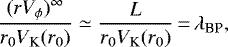
 (30)
(30)
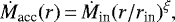
which depends on the radial distribution of magnetic field in the disk (see Appendix A). The wind outflow rate from an elementary disk annulus at radius r is then given by mass conservation as
 (31)
(31)
and the angular momentum flux extracted from the same annulus is (by definition of λBP)
![Mathematical equation: \begin{eqnarray*} \frac{\textrm{d} \dot{J}_{\textrm{DW}}(r)}{\textrm{d}r} &=& \left[\lambda_{\textrm{BP}} r V_{\textrm{K}}(r) \right] \frac{\textrm{d} \dot{M}_{\textrm{DW}}(r)}{\textrm{d}r} \\ &=& \xi \lambda_{\textrm{BP}} \dot{M}_{\textrm{in}} \sqrt{G M_{\star} / r_{\textrm{in}}} (r/r_{\textrm{in}})^{\xi -1/2}. \end{eqnarray*}](/articles/aa/full_html/2020/08/aa34377-18/aa34377-18-eq57.png)
Integration between rin and rout then gives
![Mathematical equation: \begin{equation*} \dot{J}_{\textrm{DW}}\,{=}\,\frac{\xi \lambda_{\textrm{BP}}}{\xi+1/2} \left[\dot{M}_{\textrm{out}} \sqrt{G M_{\star} r_{\textrm{out}}} - \dot{M}_{\textrm{in}} \sqrt{G M_{\star} r_{\textrm{in}}}\right]. \end{equation*}](/articles/aa/full_html/2020/08/aa34377-18/aa34377-18-eq58.png) (34)
(34)
Comparing with Eq. (29), we see that the fraction fJ of disk angular momentum extraction performed vertically by the MHD DW (as opposed to radially by turbulent or wave torques) is simply given by
 (35)
(35)
The value of ξ in a real disk is not directly measurable. However, in a steady state, it may be related to the observable mass ejection-to-accretion ratio fM through:
![Mathematical equation: \begin{equation*}f_{\textrm{M}} \equiv \frac{\dot{M}_{\textrm{DW}}}{\dot{M}_{\textrm{in}}}\,{=}\,\left[ \left(\frac{\dot{M}_{\textrm{out}}}{\dot{M}_{\textrm{in}}} \right) - 1\right]\,{=}\,\left[ \left(\frac{r_{\textrm{out}}}{r_{\textrm{in}}}\right)^{\xi} - 1\right], \end{equation*}](/articles/aa/full_html/2020/08/aa34377-18/aa34377-18-eq60.png) (36)
(36)
where we have used mass conservation (ṀDW = Ṁout – Ṁin) and the definition of ξ (Eq. (30)). We note that fM could be much larger than unity ifξ large and/or rout/rin ≫ 1.
Using the above formula to eliminate ξ from Eq. (35), we obtain the exact expression of fJ solely as a function of observable disk wind properties:
![Mathematical equation: \begin{equation*}f_J\,{=}\,\lambda_{\textrm{BP}} \times \left[ {1+ \frac{ \ln (r_{\textrm{out}}/r_{\textrm{in}}) }{2 \ln (1+f_{\textrm{M}})} } \right]^{-1}. \end{equation*}](/articles/aa/full_html/2020/08/aa34377-18/aa34377-18-eq61.png) (37)
(37)
An approximate expression for fJ may be obtained in the limits of small mass-fluxes fM ≪ 1 and large magnetic lever arms λBP ≫ 1. Equation (36) may then be approximated as
 (38)
(38)
while Eq. (35) may be rewritten as
 (39)
(39)
Combining Eqs. (39) and (38) yields
![Mathematical equation: \begin{equation*}f_J\,{\simeq}\,2 \xi \lambda_{\textrm{BP}}\,{\simeq}\,\left[\frac{2} { \ln (r_{\textrm{out}}/r_{\textrm{in}}) }\right] \lambda_{\textrm{BP}} f_{\textrm{M}}. \end{equation*}](/articles/aa/full_html/2020/08/aa34377-18/aa34377-18-eq64.png) (40)
(40)
If the wind torque dominates the disk angular momentum extraction (i.e., fJ ≃ 1) we then recover the well-known and widely used rule of thumb fM ≃ 1∕λBP (Pelletier & Pudritz 1992; Bacciotti et al. 2002; Pudritz et al. 2007). We stress, however, that Eq. (40) has an extra numerical factor in front, that depends on the wind radial extent and will generally differ from 1.
Unfortunately, the approximation in Eq. (40) is no longer valid for the small magnetic lever arms λBP ≤ 5 and large fM ≃ 1 favored by ALMA-like observations, and by nonideal MHD simulations of PPDs (Béthune et al. 2017; Bai 2017). Therefore, the Eq. (37) should preferably be used to accurately evaluate fJ in disk wind candidates.
We now proceed to obtain an observational estimate of fM in HH212. Considering first ṀDW, Lee et al. (2018a) estimated the mass in the rotating SO-rich disk outflow within z ≤0.′′2 ≃ 90 au from the source at (0.4−4) × 10−4M⊙, where the range of a factor ten reflects the current uncertainty in SO abundance in this flow (Podio et al. 2015). Scaling to our adopted distance of 450 pc, and taking the mean vertical velocity Vz ≃ 10 km s−1 of the best fit MHD DW model, the wind-crossing time through this region is ≃ 50 yr, and the corresponding ejected-mass flux is ṀDW ≃ 1−10 × 10−6M⊙ yr−1. We now estimate the accretion rate onto the HH212 source: since it is a young Class 0 protostar, we expect it to lie along the “birthline” where stellar radius grows over time (Stahler 1988). For a stellar mass M⋆ ≃ 0.25 M⊙ (Lee et al. 2017b), the observed bolometric luminosity of 11 L⊙ (Zinnecker et al. 1992, scaled to our adopted distance of 450 pc) is reached for an accretion rate onto the star of Ṁ⋆ ≃ 2 × 10⁻⁶ M⊙ yr−1 (see Fig. 9 in Stahler 1988). The high-velocity axial SiO/CO jet ejected from within ≃ 0.1 au of the source (Lee et al. 2017a; Tabone et al. 2017) removes an additional Ṁjet ≃ 10−6 M⊙ yr−1 from the incoming accretion flow (Lee et al. 2015). Therefore, in steady state the disk accretion rate at rin = 0.1 au is Ṁin = Ṁ⋆ + Ṁjet ≃ 3 × 10⁻⁶M⊙ yr−1.
From the above observational estimates of ṀDW and Ṁin we infer an ejection-to-accretion ratio of fM,obs = ṀDW/ Ṁin = 0.33–3.3. Inserting these values into Eq. (37) and taking rin = 0.1 au, rout = 40 au, and λBP = 5.5 from PV cut modeling (see Figs. 11, 12 and Tabone et al. 2017), we obtain fJ,obs = 0.5–1.8. We note that despite the large uncertainty on the SO abundance, we find fJ,obs ≥ 0.5. In other words,the angular momentum flux extracted by the proposed MHD DW candidate in HH212 agrees within a factor two with that required to sustain accretion through the whole disk at the current observed rate.
5 Conclusions
We studied observational biases in the rotation signatures of radially extended MHD disk winds when observed at the typical resolution oflarge millimeter interferometers such as ALMA. We then tested our predictions for the edge-on case against published ALMA observations of HH212 covering a factor 15 in angular resolution. Our main results can be summarized as follows.
The launch radius robs inferred using Anderson’s formula from rotation signatures in transverse PV cuts generally differs markedly from the true outermost launch radius of the MHD DW, rout. The sign of this bias depends on the method used to estimate the flow specific angular momentum from PV cuts, opening the possibility to bracket the true value of rout. In the double-peak separation method applied to edge-on PV cuts (Sect. 3.2.1), robs always underestimates the true rout. This bias does not become smaller at higher angular resolution, and becomes greater with the wind radial extension and emissivity gradient, reaching a factor of between three and ten for typical parameters. At lower inclinations where the two PV peaks have the same velocity sign, this method becomes unreliable and should be avoided. The apparent flow width method (see Sect. 3.2.3) suffers a similar bias to the double-peak separation in edge-on PV cuts, and also provides a strict lower limit to the true rout, available at all flow inclinations. The rotation curve method (see Sect. 3.2.2) only yields a good estimate of rout when the flow is well resolved transversally. Otherwise, it provides an upper limit to rout by an increasing amount for stronger beam smearing.
The magnetic lever arm inferred from apparent rotation signatures using Anderson’s formula is not as strongly impacted by observational biases (which tend to cancel out in the calculation). However, due to unobservable angular momentum in the form of magnetic field torsion, it only gives a strict lower limit to the true Blandford & Payne magnetic lever arm parameter λBP (as already pointed out in the context of T Tauri jets by Pesenti et al. 2004; Ferreira et al. 2006). In our model, this “MHD bias” becomes significant for zcut/rout < 20, where zcut is the altitude of the PV cut. The true λBP can then only be constrained through detailed modeling of PV cuts.
While our analysis is limited to self-similar models, we expect similar biases to occur in more general geometries (see e.g., Pudritz et al. 2007, or a conical wind) whenever the same underlying causes are present (i.e., strong contrast effects between inner and outer streamlines and beam smearing). However, the biases might change if the internal velocity gradients are strongly non-Keplerian. We defer the study of these more general cases to future work.
Our main results for the double-peaked PV method were tested against ALMA observations of the edge-on flow in HH212 at angular resolutions from 250 to 18 au, which provide the most stringent observational test of MHD DW models to date. We verified thatthe PV double-peak separation indeed does not depend on beam size, and find that the launch radius robs ≃ 1 au inferred from it using Anderson’s relation strongly underestimates the true outermost launch radius of the flow, directly resolved at rout ≃ 40 au in the 18 au ALMA data. We also showed that the MHD DW model for HH212 proposed by Tabone et al. (2017) still reproduces the main features of transverse PV cuts at four times lower and higher resolution quite well (given its idealized self-similar geometry). However, the poloidal velocity is not well constrained in such an edge-on view, and alternative interpretations in terms of wind-driven or bowshock-driven shells are also possible (Lee et al. 2018a; Tabone et al. 2018).
The fraction of disk angular momentum flux extracted by a steady self-similar MHD DW is derived as a function of rin, rout, λBP, and the observed mass ejection-to-accretion ratio fM (see Eq. (37)). Application to HH212 supports the proposed paradigm where MHD DWs drive accretion across protoplanetary disks.
Observing rotating winds with less edge-on inclinations (where the distribution of Vz can be better constrained) will be crucial to help discriminate between MHD DWs and alternative explanations (e.g., wide-angle wind cavities) and definitively elucidate the mechanism driving disk accretion in protostars. Searches for pristine MHD DW signatures should focus on regions very close to the source with the highest possible angular resolution in order to avoid large-scale bowshocks driven by the axial jet and interactions with the infalling envelope.
Acknowledgements
We are grateful to C. Dougados for useful suggestions, and to an anonymous referee for constructive comments that helped to improve the manuscript presentation and content. This paper makes use of the ALMA 2012.1.00997.S and 2016.1.01475.S data (PI: C. Codella). ALMA is a partnership of ESO (representing its member states), NSF (USA), and NINS (Japan), together with NRC (Canada) and NSC and ASIAA (Taiwan), in cooperation with the Republic of Chile. The Joint ALMA Observatory is operated by ESO, AUI/NRAO, and NAOJ. This work was supported by the Programme National Physique et Chimie du Milieu Interstellaire (PCMI) of CNRS/INSU with INC/INP and co-funded by CNES, and by the Conseil Scientifique of Observatoire de Paris. B.T. acknowledges funding from the research programme Dutch Astrochemistry Network II with project number 614.001.751, which is financed by the Dutch Research Council (NWO). E.B. and C.C. acknowledge funding from the European Research Council (ERC) under the European Union’s Horizon 2020 research and innovation programme, for the Project “The Dawn of Organic Chemistry” (DOC), grant agreement No 741002. This research has made use of NASA’s Astrophysics Data System.
Appendix A Parameters and properties of MHD DW solutions
The self-similar, stationary, and axisymmetric MHD disk-wind solutions computed for this work treat the disk accretion and ejection processes in an exact and consistent manner, using the formalism and method described in Ferreira (1997); Casse & Ferreira (2000a). The vertical, radial, and rotational balance equations of the resistive, viscous, and magnetized accreting disk are integrated through a set of coupled ODEs and determine the emerging jet parameters and the large-scale collimation. Consequently, in order to compute an MHD disk wind solution, several free input disk parameters have to be set that describe the disk thermal scale height, viscosity, resistivity, and magnetic field structure. For information and reference purposes, the disk parameter values used to obtain the four solutions used in this work are listed in Table A.1, and the definition of each parameter is given at the end of this section. Following Casse & Ferreira (2000b), a (self-similar) heating function in the disk atmosphere is implemented to mimic coronal heating along magnetic surfaces, which allows us to enhance the wind mass-loading compared to isothermal or adiabatic solutions. The heating function adopted for each of the four MHD DW solutions is plotted in Fig. A.1. The variations of density and magnetic field along magnetic surfaces in our four solutions are presented in Fig. A.2.
Disk parameters and emerging wind properties of the calculated self-similar MHD solutions.
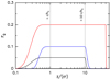 |
Fig. A.1 Vertical profile of the normalized entropy generation function FQ(z∕ɛr) in the four computed MHD disk wind solutions. In blue L13W36, in black L13W120, in red the (identical) function for L5W17 and L5W30. FQ is related to the entropy source function along the magnetic flow surface through |

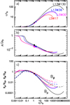 |
Fig. A.2 Variation of a: radius, b: density ρ, and c: poloidal and toroidal magnetic field (in solid and dashed curves respectively) along a magnetic wind surface as a function of z∕r0, for the four computed MHD DW solutions. The Alfvén point for each solution is plotted as a filled dot. Quantities are normalized by the mid-plane value of radius, density, and vertical magnetic field Bz,0 at r0. The latter are related to the dimensional parameters of the system through
|

Here, we consider solutions where the MHD DW extracts most of the angular momentum required for disk accretion, with negligible contribution from the viscous torque. However, Casse & Ferreira (2000a) showed that it is possible to obtain identical emerging jetconfigurations with a smaller ratio of wind to turbulent torques. Hence, the emerging wind properties in our solutions are actually relevant for a much broader range of situations.
The nondimensional parameters describing the self-similar disk structure are defined as follows and are listed in Table A.1 (see Casse & Ferreira 2000a, for further details):
The ejection efficiency
 is related to the radial scaling of the mid-plane magnetic field
  through αB = −5∕4 + ξ∕2.
The disk thermal aspect ratio ɛ ≡ h(r0)∕r0 ≡ cS∕VK(r0) where h(r0) is the disk vertical pressure scale height, VK the Keplerian rotation speed, and cS the sound speed at radius r0 in the disk midplane.
The Shakura-Sunyaev viscosity parameter in the disk midplane,
 with νv the (anomalous) effective viscosity.
The poloidal magnetic diffusivity parameter at the disk mid-plane,
 with νm the (anomalous) poloidal magnetic diffusivity and VA the Alfven speed.
The magnetic diffusivity anisotropy
 where
where  is the toroidal magnetic diffusivity.
The disk mid-plane magnetization
 =
=  where P is the thermal pressure and Bz the magnetic field in the disk mid-plane (2∕μ is the usual plasma parameter β).
The inclination of the magnetic field at the disk surface
 , where
  is the magnetic Reynolds number in the mid-plane and
  and
and  are the radial and vertical magnetic fields at the disk surface.
The magnetic shear
 where
where  is the toroidal magnetic field at the disk surface.
For computational reasons, ξ, ɛ, αv, αm and χm are taken as free input parameters, while μ and p are numerically adjusted in order to cross the slow and Alfvén critical points, respectively. The value of q is inferred from the other disk parameters and is only given in Table A.1 for the sake of completeness. To limit the number of free parameters, we assumed that the viscosity νv and resistivity νm are equal (i.e., a magnetic Prandl number ≃1), since they are both “anomalous” transport coefficients arising presumably from the same turbulence. This assumption corresponds to  . It does not affect our solutions, where the turbulent viscous torque (included in our equations) is much smaller than the dominant disk wind torque.
Appendix B Transverse PV diagram for a rotating and expanding wind annulus
Here, we show that the transverse PV diagram produced by a single axisymmetric wind annulus observed at inclination i to the line of sight is an ellipse. We describe extremal points of interest on the ellipse, and relate the parameters of the ellipse (semi-major and semi-minor axes, PA, central velocity) to the physical parameters of the annulus (radius, Vr, Vϕ, Vz). In Appendix B.2 we then investigate the effect of spatial and velocity smearing on the location of intensity peaks in the PV diagram.
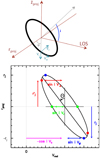 |
Fig. B.1 Top: schematic view of a thin wind annulus of radius rj, expansion velocity Vr, azimuthal velocity Vϕ, and vertical velocity Vz along the jet axis, inclined by an angle i from the line of sight. A point on this annulus is located by the azimuthal angle ϕ. Bottom: the transverse PV diagram for the wind annulus is an ellipse (in black) centered on rproj = 0 and Vrad = − cosiVz, of minor andmajor axes and tilt angle Θ given by Eqs. B.8 and B.9. Three pairs of points of interest are indicated: the on-axis points (in green) giving the projected Vr ; the points of maximum radii (in blue) giving the projected Vϕ; and the points of maximum radial velocity (in red) with |

B.1 Ellipse shape and tilt for a single wind annulus
We consider a thin axisymmetric annulus of radius rj with a vertical outflow velocity Vz, rotation velocity Vϕ, and radial expansion velocity Vr, observed at an inclination angle i with respect to the line ofsight (i = 0 corresponds to a face-on ring). We show in Fig. B.1(top) a schematic view of the annulus and the adopted coordinate system. The projected position rproj(ϕ) and projected radial velocity Vrad(ϕ) of an elementary segment located at azimuthal angle ϕ are given by
![Mathematical equation: \begin{eqnarray*} r_{\textrm{proj}}(\phi) &=& \cos{\phi} ~ r_j, \\[2pt] V_{\textrm{rad}}(\phi) &=& -\left(\cos{i}~V_z +\sin{i}\sin{\phi}~V_r +\sin{i}\cos{\phi}V_{\phi}\right), \end{eqnarray*}](/articles/aa/full_html/2020/08/aa34377-18/aa34377-18-eq80.png)
where we adopt the usual astrophysical convention of negative radial velocity for approaching material. Denoting the magnitude of the transverse velocity (in the plane perpendicular to the flow axis) as
 (B.3)
(B.3)
and making the change of variable V = (Vrad + cosi Vz)∕sin i, we obtain a quadratic equation in V and rproj
 (B.4)
(B.4)
This equation defines an ellipse in the PV diagram, centered on rproj = 0 and Vrad = −cosiVz. This ellipse is shown in Fig. B.1 (bottom) for our reference case where Vz < 0 (redshifted lobe of the jet). Three pairs of point on this ellipse are of particular interest.
-
First, towards the projected jet axis at rproj = 0 (i.e. for ϕ = ± π∕2), the line-of-sight component of the rotation velocity cancels out and Vrad = −Vz cosi ± Vr sin i (green dots in Fig. B.1).
-
Second, towards the maximum projected radius rproj = rj where the line of sight is tangent to the annulus (i.e., for ϕ = 0 or ϕ = π) the line-of-sight component of the expansion velocity Vr vanishes and Vrad = −Vz cosi ± Vϕ sin i (blue dots in Fig. B.1).
-
Third, and most importantly, the points where the ellipse reaches its minimum and maximum projected velocities (red dots in Fig. B.1) are located at rproj = ±(Vϕ∕V⊥)rj and Vrad = −Vz cosi ± V⊥sin i.
In the following, we assume for simplicity an edge-on flow with sin i = 1. Denoting as  ,
,  , and
, and  , the (dimensionless) numerical values of jet radius and velocities in the chosen units of the graph axes (e.g., au and km s−1), and diagonalizing Eq. (B.4), we obtain that the PV ellipse has a semi-major axis a and semi-minor axis b (in dimensionless graph units) given by:

The tilt angle Θ of the ellipse in the PV diagram, measured from the increasing rproj axis towards the decreasing radial velocity axis (see Fig. B.1), is such that
 (B.9)
(B.9)
The general expressions for random inclinations can be recovered by multiplying  ,
,  , and
, and  by sin i in these expressions. The reverse relations allowing to calculate rj, Vr, and Vϕ from the ellipse parameters a, b, and Θ may be found in Appendix B of Louvet et al. (2018), where Θ is denoted as PA.
B.2 Impact of spatial and velocity smearing on emission peak positions
We now examine the influence of spatial and velocity smearing on the separation of emission peaks in the elliptical PV of a single annulus, assuming an optically thin line. We simply add up the emission contributions of each elementary arc dϕ to the corresponding velocity/position bins in the PV diagram. The PV is then smoothed by a Gaussian beam of FWHM = θb and by a velocity broadening of FWHM = δV. We find that the synthetic PV diagrams always present two symmetric peaks, whose positions (V1, r1) and (V2, r2) depend on the ratios θb∕rj and δV∕V⊥. Four cases are identified, which are displayed in Fig. B.2:
-
(a) δV∕V⊥≪ θb∕rj (Fig. B.2a): when the jet is better resolved spectrally than spatially (as usually the case for millimeter interferometric observations) the intensity peaks are located at the points of extremum velocities along the ellipse (red dots in Fig. B.2):

In that case, the spatial shift between emission peaks, Δr ≡ r1 − r2 = 2rj(Vϕ∕V⊥) is smaller than the true ring diameter 2rj, while the velocity shift between emission peaks ΔV = 2sin iV⊥ is larger than 2Vϕ sin i. Yet, the (inclination-corrected) specific angular momentum that one would estimate from the spatial and velocity separations of PV peaks,
 (B.12)
is still equal to the true specific angular momentum of the elementary rotating annulus, jout = rjVϕ, since the terms in V⊥ cancel out in the product.
-
(b) θb∕rj ≪ δV∕V⊥ (Fig. B.2b): Conversely, when the jet is better resolved spatially than spectrally (as e.g. in optical/near-IR observations of the DG Tau jet), the peaks are located at the points of extremum radii on the ellipse (blue dots in Fig. B.2) at

In that (simpler) case, the spatial shift between peaks Δr gives directly the true diameter of the annulus, the velocity shift ΔV gives directly the true projected rotation velocity 2sin iVϕ. Like in case a), the apparent (inclination corrected) specific angular momentum jobs is equal to the true value in the ring.
-
(c) θb∕rj ~ δV∕V⊥≪ 1 (Fig. B.2c): when the jet is similarly well resolved spatially and spectrally, the two emission peaks lie on the ellipse somewhere between the extremal velocity and radial points (i.e. between the red and blue dots). In this case as well, jobs will be close to the true jout.
-
(d) θb∕rj ~ δV∕V⊥~ 1 (Fig. B.2d): when the jet is under-resolved both spatially and spectrally, the two emission peaks migrate inwards, roughly along the ellipse PA angle. In this last case, the apparent specific angular momentum jobs will underestimate the true value in the ring.
In summary, as long as the emitting ring is narrow and well resolved in at least one dimension (spatial or spectral), and S/N is high enough to measure the centroid shift below the beam scale in the other dimension (using e.g., spectro-astrometric techniques or cross-correlation), jobs estimated from PV peak separations using Eq. (B.12) gives a good estimate of the true specific angular momentum in the ring, jout.
However, this conclusion is only valid for a narrow emitting ring. For a radially extended disk wind, where we observe the summed contribution of a broad range of nested rings, the situation is more complex. When the flow is close to edge-on, we find that jobs estimated from PV double-peak separations always significantly underestimates jout even at high spectral and angular resolutions (see Sect. 3.3.1). Below some critical inclination angle icrit ≃ arctan∣V⊥∣∕Vϕ the PV is no longer systematically double peaked and other methods must be used to estimate the flow specific angular momentum (see Sect. 3.2).
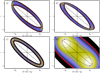 |
Fig. B.2 Effect of spatial beam (θb) and spectral broadening (δV) on peak separation in synthetic transverse PV diagrams for an expanding and rotating annulus of radius rj and Vϕ = 3 × Vr. Panel a: significant beam smearing θb = 0.2 × rj but negligible line broadening δV ≪ Vr: peaks on velocity extrema (red dots); this is the case expected for ALMA observations of cool molecular disk winds. Panel b: significant line broadening δV = 0.2× Vϕ but negligible beam convolution θb ≪ rj: peaks on spatial extrema (blue dots). Panel c: high spatial and velocity resolution (θb = 0.1× rj, δV = 0.1× Vϕ): peaks between red and blue dots, close to the ellipse major axis; panel d: low spatial and spectral resolution θb ∕rj = δV∕Vϕ = 1: peaks move closer in, along the ellipse PA. |
References
- Anderson, J. M., Li, Z.-Y., Krasnopolsky, R., & Blandford, R. D. 2003, ApJ, 590, L107 [NASA ADS] [CrossRef] [Google Scholar]
- Bacciotti, F., Ray, T. P., Mundt, R., Eislöffel, J., & Solf, J. 2002, ApJ, 576, 222 [NASA ADS] [CrossRef] [Google Scholar]
- Bai, X.-N. 2017, ApJ, 845, 75 [NASA ADS] [CrossRef] [Google Scholar]
- Bai, X.-N., & Stone, J. M. 2013, ApJ, 769, 76 [NASA ADS] [CrossRef] [Google Scholar]
- Balbus, S. A., & Hawley, J. F. 1991, ApJ, 376, 214 [NASA ADS] [CrossRef] [Google Scholar]
- Béthune, W., Lesur, G., & Ferreira, J. 2017, A&A, 600, A75 [NASA ADS] [CrossRef] [EDP Sciences] [Google Scholar]
- Bianchi, E., Codella, C., Ceccarelli, C., et al. 2017, A&A, 606, L7 [NASA ADS] [CrossRef] [EDP Sciences] [Google Scholar]
- Bjerkeli, P., van der Wiel, M. H. D., Harsono, D., Ramsey, J. P., & Jørgensen, J. K. 2016, Nature, 540, 406 [NASA ADS] [CrossRef] [Google Scholar]
- Blandford, R. D., & Payne, D. G. 1982, MNRAS, 199, 883 [NASA ADS] [CrossRef] [Google Scholar]
- Cabrit, S., Pety, J., Pesenti, N., & Dougados, C. 2006, A&A, 452, 897 [NASA ADS] [CrossRef] [EDP Sciences] [Google Scholar]
- Casse, F., & Ferreira, J. 2000a, A&A, 353, 1115 [NASA ADS] [Google Scholar]
- Casse, F., & Ferreira, J. 2000b, A&A, 361, 1178 [NASA ADS] [Google Scholar]
- Chen, X., Arce, H. G., Zhang, Q., Launhardt, R., & Henning, T. 2016, ApJ, 824, 72 [NASA ADS] [CrossRef] [Google Scholar]
- Codella, C., Bianchi, E., Tabone, B., et al. 2018, A&A, 617, A10 [NASA ADS] [CrossRef] [EDP Sciences] [Google Scholar]
- Coffey, D., Bacciotti, F., Ray, T. P., Eislöffel, J., & Woitas, J. 2007, ApJ, 663, 350 [NASA ADS] [CrossRef] [Google Scholar]
- Coffey, D., Dougados, C., Cabrit, S., Pety, J., & Bacciotti, F. 2015, ApJ, 804, 2 [NASA ADS] [CrossRef] [Google Scholar]
- Combet, C., & Ferreira, J. 2008, A&A, 479, 481 [NASA ADS] [CrossRef] [EDP Sciences] [Google Scholar]
- de Valon, A., Dougados, C., Cabrit, S., et al. 2020, A&A, 634, L12 [NASA ADS] [CrossRef] [EDP Sciences] [Google Scholar]
- Fendt, C. 2011, ApJ, 737, 43 [NASA ADS] [CrossRef] [Google Scholar]
- Ferreira, J. 1997, A&A, 319, 340 [Google Scholar]
- Ferreira, J. 2001, Dossier Pour La Science, 30, 80 [Google Scholar]
- Ferreira, J., & Pelletier, G. 1995, A&A, 295, 807 [NASA ADS] [Google Scholar]
- Ferreira, J., Dougados, C., & Cabrit, S. 2006, A&A, 453, 785 [NASA ADS] [CrossRef] [EDP Sciences] [Google Scholar]
- Hartmann, L., Herczeg, G., & Calvet, N. 2016, ARA&A, 54, 135 [NASA ADS] [CrossRef] [Google Scholar]
- Hirota, T., Machida, M. N., Matsushita, Y., et al. 2017, Nat. Astron., 1, 0146 [Google Scholar]
- Jacquemin-Ide, J., Ferreira, J., & Lesur, G. 2019, MNRAS, 490, 3112 [CrossRef] [Google Scholar]
- Konigl, A. 1989, ApJ, 342, 208 [NASA ADS] [CrossRef] [Google Scholar]
- Kounkel, M., Hartmann, L., Loinard, L., et al. 2017, ApJ, 834, 142 [NASA ADS] [CrossRef] [Google Scholar]
- Launhardt, R., Pavlyuchenkov, Y., Gueth, F., et al. 2009, A&A, 494, 147 [NASA ADS] [CrossRef] [EDP Sciences] [Google Scholar]
- Lee, C.-F., Stone, J. M., Ostriker, E. C., & Mundy, L. G. 2001, ApJ, 557, 429 [NASA ADS] [CrossRef] [Google Scholar]
- Lee, C.-F., Ho, P. T. P., Bourke, T. L., et al. 2008, ApJ, 685, 1026 [NASA ADS] [CrossRef] [Google Scholar]
- Lee, C.-F., Hirano, N., Zhang, Q., et al. 2014, ApJ, 786, 114 [NASA ADS] [CrossRef] [Google Scholar]
- Lee, C.-F., Hirano, N., Zhang, Q., et al. 2015, ApJ, 805, 186 [NASA ADS] [CrossRef] [Google Scholar]
- Lee, C.-F., Ho, P. T. P., Li, Z.-Y., et al. 2017a, Nat. Astron., 1, 0152 [NASA ADS] [CrossRef] [Google Scholar]
- Lee, C.-F., Li, Z.-Y., Ho, P. T. P., et al. 2017b, ApJ, 843, 27 [NASA ADS] [CrossRef] [Google Scholar]
- Lee, C.-F., Li, Z.-Y., Codella, C., et al. 2018a, ApJ, 856, 14 [NASA ADS] [CrossRef] [Google Scholar]
- Lee, C.-F., Li, Z.-Y., Hirano, N., et al. 2018b, ApJ, 863, 94 [NASA ADS] [CrossRef] [Google Scholar]
- Louvet, F., Dougados, C., Cabrit, S., et al. 2016, A&A, 596, A88 [NASA ADS] [CrossRef] [EDP Sciences] [Google Scholar]
- Louvet, F., Dougados, C., Cabrit, S., et al. 2018, A&A, 618, A120 [NASA ADS] [CrossRef] [EDP Sciences] [Google Scholar]
- Ogihara, M., Kokubo, E., Suzuki, T. K., & Morbidelli, A. 2018, A&A, 615, A63 [NASA ADS] [CrossRef] [EDP Sciences] [Google Scholar]
- Panoglou, D., Cabrit, S., Pineau Des Forêts, G., et al. 2012, A&A, 538, A2 [NASA ADS] [CrossRef] [EDP Sciences] [Google Scholar]
- Pelletier, G., & Pudritz, R. E. 1992, ApJ, 394, 117 [NASA ADS] [CrossRef] [Google Scholar]
- Pesenti, N., Dougados, C., Cabrit, S., et al. 2004, A&A, 416, L9 [NASA ADS] [CrossRef] [EDP Sciences] [Google Scholar]
- Podio, L., Codella, C., Gueth, F., et al. 2015, A&A, 581, A85 [NASA ADS] [CrossRef] [EDP Sciences] [Google Scholar]
- Pudritz, R. E., & Norman, C. A. 1983, ApJ, 274, 677 [NASA ADS] [CrossRef] [Google Scholar]
- Pudritz, R. E., Ouyed, R., Fendt, C., & Brandenburg, A. 2007, in Protostars and Planets V, eds. B. Reipurth, D. Jewitt, & K. Keil (Tucson: University of Arizona Press), 277 [Google Scholar]
- Sauty, C., Cayatte, V., Lima, J. J. G., Matsakos, T., & Tsinganos, K. 2012, ApJ, 759, L1 [NASA ADS] [CrossRef] [Google Scholar]
- Shu, F. H., Najita, J. R., Shang, H., & Li, Z. Y. 2000, in Protostars and Planets IV, eds. V. Mannings, A. P. Boss, & S. S. Russell (Tucson: University of Arizona Press), 789 [Google Scholar]
- Staff, J. E., Koning, N., Ouyed, R., Thompson, A., & Pudritz, R. E. 2015, MNRAS, 446, 3975 [NASA ADS] [CrossRef] [Google Scholar]
- Stahler, S. W. 1988, ApJ, 332, 804 [NASA ADS] [CrossRef] [Google Scholar]
- Tabone, B., Cabrit, S., Bianchi, E., et al. 2017, A&A, 607, L6 [NASA ADS] [CrossRef] [EDP Sciences] [Google Scholar]
- Tabone, B., Raga, A., Cabrit, S., & Pineau des Forêts, G. 2018, A&A, 614, A119 [NASA ADS] [CrossRef] [EDP Sciences] [Google Scholar]
- Tabone, B., Godard, B., Pineau des Forêts, G., Cabrit, S., & van Dishoeck, E. F. 2020, A&A, 636, A60 [CrossRef] [EDP Sciences] [Google Scholar]
- Turner, N. J., Fromang, S., Gammie, C., et al. 2014, in Protostars and Planets VI, eds. H. Beuther, R. S. Klessen, C. P. Dullemond, & T. Henning (Tucson: University of Arizona Press), 411 [Google Scholar]
- Yvart, W., Cabrit, S., Pineau des Forêts, G., & Ferreira, J. 2016, A&A, 585, A74 [NASA ADS] [CrossRef] [EDP Sciences] [Google Scholar]
- Zapata, L. A., Schmid-Burgk, J., Muders, D., et al. 2010, A&A, 510, A2 [NASA ADS] [CrossRef] [EDP Sciences] [Google Scholar]
- Zapata, L. A., Lizano, S., Rodríguez, L. F., et al. 2015, ApJ, 798, 131 [NASA ADS] [CrossRef] [Google Scholar]
- Zhang, Y., Higuchi, A. E., Sakai, N., et al. 2018, ApJ, 864, 76 [NASA ADS] [CrossRef] [Google Scholar]
- Zinnecker, H., Bastien, P., Arcoragi, J.-P., & Yorke, H. W. 1992, A&A, 265, 726 [NASA ADS] [Google Scholar]
An extra term (h − h0) must then be added to the right-hand side of Eq. (1), where h and h0 are the specific enthalpy at the observation point and at the flow base, respectively. Counter-rotation (VϕΩ0 < 0) results if  , meaning that the enthalpy gradient dominates the flow kinematics.
In an enthalpy-driven MHD DW, the extra term (h0 − h) would be too poorly known; in a nonsteady or nonaxisymmetric MHD DW, the MHD invariants used to derive Eq. (1) would no longer hold.
Which assumes that the variation of a given quantity with polar angle θ is the same for all streamlines, while the variation with radius is a power law.
The variation of ɛ with z has little influence on transverse PV cuts as long as this variation is smooth over the scales probed by the beam. Here we take a dependence of the form e−z∕H with H = 600 au for illustrative purposes.
This expression is similar to Eq. (5) except that it involves the total velocity modulus instead of the asymptotic poloidal velocity
 , and the local λϕ
instead of λBP.
, and the local λϕ
instead of λBP.
That could be easily produced e.g. by a slightly steeper abundance or excitation gradient on larger scales.
The bright SO2 line at 334.67335 GHz observed by Tabone et al. (2017) was not covered by the spectral setup of Lee et al. (2018a), who instead stacked 12 weak SO2 lines; since stacking adds some uncertainty due to the limited spectral resolution, we focus here on the SO line common to the two studies.
All Tables
Disk parameters and emerging wind properties of the calculated self-similar MHD solutions.
All Figures
|
Fig. 1 Poloidal cut of a self-similar, axisymmetric MHD DW for our reference solution (L5W17). Selected flow surfaces are plotted in red. Four important model parameters affecting predictedrotational signatures are illustrated here: the inner and outer launching radii, rin and rout, of the wind-emitting region (taken as 0.5 au and 8 au in this graph); the magnetic lever arm parameter λBP (here = 5.5)
|
| In the text | |
|
Fig. 2 Shape and kinematics of the streamlines as a function of vertical distance z above the disk midplane for the four computed MHD DW solutions in Table 1. a: cylindrical radius r, b: velocity along the jet axis Vz, c: azimuthal rotation velocity Vϕ, d: radial expansion velocity Vr. Filled dots indicate the Alfvén surface. Distances are scaled by the launch radius r0, and velocities by the Keplerian speed at r0, VK (r0). Models are denoted as LxWy with x = λBP the magnetic lever arm parameter and y = |
| In the text | |
|
Fig. 3 a: definition of inclination angle i for our synthetic predictions in Sect. 3. b: sketch illustrating the construction of the transverse PV cut at projected altitude zcut with a Gaussian beam θb. Wind rotation induces different line-of-sight velocities at symmetric offsets + r and − r on either side of the jet axis, producing a detectable “tilt” in the PV cut (see Fig. 4). This projected velocity shift is used to estimate the rotation speed and specific angular momentum of the flow (see Sect. 3.2). Adapted from Ferreira (2001). |
| In the text | |
|
Fig. 4 a: on-axis spectrum and transverse PV diagram for the reference model viewed at i = 87°, illustratingthe “edge-on” case. The two red dots indicate the intensity peaks in the PV, which have opposite velocity signs in this configuration; their connecting line defines the spatial and velocity separations Δr and ΔV used to estimate the observed specific angular momentum jobs in Eq. (15). We also plot in black the ellipse and peak positions contributed by the outermost streamline alone, which predict a similar velocity shift ΔVth (see Eq. (13)) but a much larger spatial shift Δrth (see Eq. (12)). Other model parameters are: zcut = 225 au, M* = 0.1 M⊙, rin = 0.25 au, rout = 8 au, α = − 2, and θb = 225 au. Filled rectangles show the spectral and angular resolutions. b: same as (a) but at lower inclination i = 70° (note the change in velocity scale) for α = 0 and θb = 225 au (red) and 45 au (blue). Double-peaks in the PV diagram now have the same velocity sign, and can vanish at moderate angular resolution. |
| In the text | |
|
Fig. 5 Double-peak separation in edge-on PVs of radially extended DWs (connected dots) compared with the theoretical value for a single wind annulus on the outermost streamline (dotted curves). Left column: observed spatial separation Δr vs. theoretical Δrth (from Eq. (12)); middle column: deprojected velocity shift ΔV ∕sin i vs. theoretical value ΔVth∕sin i (from Eq. (13)). Right column: ratio of the apparent specific angular momentum jobs = (Δr∕2) × (ΔV∕2sin i) to the true value on the outermost streamline, jout = (Δrth ∕2) × (ΔVth∕2sin i). From top to bottom panels: the influence of varying (a) MHD solution (colour-coded) and inclination angle; (b) outermost launching radius rout of the emitting region of the MHD DW; (c) index α of the emissivity radial power law (see Eq. (8)); and (d) spatial beamFWHM θb and PV cut position zcut. All nonlabeled model parameters are fixed at their reference value: i = 87°, MHD solution = L5W17, rout = 8 au, α = − 2, θb = 225 au, zcut = 225 au, M⋆ = 0.1 M⊙, and rin = 0.25 au. Datapoints for this reference case are circled in orange in each panel. |
| In the text | |
|
Fig. 6 Comparisons of synthetic on-axis spectra and transverse PV cuts at zcut = 225 au for selected pairs of quasi edge-on models that differ by only one parameter at a time. In red, we show the reference model with i = 87°, rout = 8 au, α = − 2 (see Eq. (8)), θb = 225 au, λBP = 5.5, and |
| In the text | |
|
Fig. 7 Observational biases in the PV double-peak separation method for our reference edge-on case (i = 87°), as a functionof the DW radial extension (for α = −2, connected red dots) and emissivity index α (for rout/rin = 32, connected green dots): panels a and b show specific angular momentum and poloidal velocity estimated from the PV double-peak separation; c and d show launch radius and magnetic lever arm parameter inferred from the observed quantities in (a) and (b) using Anderson’s relations (Eqs. (1) and (2)). Values that would be obtained for a single ring on the outermost wind streamline are shown in dotted red curves. The true magnetic lever arm parameter λBP of the MHD solution and relevant values at rin are indicated for reference in dot-dashed blue. |
| In the text | |
|
Fig. 8 “Observed” rotation curve Vϕ,obs(r) obtained from the difference of peak velocity between ± r from the jet axis (Eq. (16)) for our reference model viewed at i = 40°, 60°, 70°, and 80° (color-coded curves). (a): Spatially resolved regime (θb = 45 au), (b): spatially unresolved regime (θb = 225 au; we note the change of scales on both axes). In both panels, a vertical black line indicates the beam FWHM, and colored vertical dashed lines indicate the flow radius rj at zcut = 225 au. The true wind rotation curve Vϕ(r) at z = zcut∕sin i) is shown by dotted curves, with a constant value beyond rj. The cross on the red curve illustrates where the local intensity drops below 10% of the PV peak. |
| In the text | |
|
Fig. 9 Examples of bias when using the rotation curve method for a representative model at i = 40° (in red in Fig. 8): “Observed” launch radii robs(r) (a) and magnetic lever arms λobs(r) (b) inferred at each r by application of Anderson’s formula to jobs(r) and Vp,obs(r) (Eqs. (25) and (26)). Green curves illustrate the spatially resolved regime (θb = 45 au) and red curves the unresolved regime (θb = 225 au). These curves stop at 1% of the PV peak intensity, with a plus symbol marking 10%. The black vertical line shows the flow radius rj. For comparison, dotted blue curves plot the true launch radii r0(r) (a) and λϕ(r) (b) of each DW streamline tangent to r; horizontal dashed blue lines mark the true outermost launch radius rout = 8 au (a) and true λBP = 5.5 (b) in the model. Other model parameters are: MHD solution L5W17, α = −2, M⋆ = 0.1 M⊙, and rin = 0.25 au. |
| In the text | |
|
Fig. 10 Rotation signatures retrieved at 225 au resolution by spectro-astrometry towards the low-velocity HH212 outflow. Blue (resp. red) contours show SO(98−87) blueshifted (resp. redshifted) emission over intermediate velocities (1.5 km s−1 < ∣ VLSR − Vsys∣ < 2.8 km s−1) mapped with ALMA Cycle 0 (from Podio et al. 2015). The blue (resp. red) dots mark the centroid positions of transverse intensity cuts at each altitude across the blue (resp. red) contour maps. The black asterisk indicates the continuum peak. The jet was rotated to point upwards for clarity. Horizontal black dashed lines depict the position of PV cuts at z ± 70 au shown in Fig. 11. The clean beam FWHM of 0.65″ × 0.47″ is shown as afilled black ellipse. First contours are 0.1 mJy beam−1 km s−1 and steps are 0.15 mJy beam−1 km s−1. |
| In the text | |
|
Fig. 11 Comparison between observed and modeled SO on-axis spectra and transverse position-velocity cuts taken at ± 0.′′15 (70 au) across the blueshifted (left panels) and redshifted (right panels) lobes of the HH212 jet. Top row: ALMA Cycle 4 data (70 au beam) from Tabone et al. (2017). Bottom row: ALMA Cycle 0 data (250 au beam) from Podio et al. (2015). In all panels, observed spectra are plotted as histograms, and observed PV diagrams are shown as color maps with white contours. Synthetic predictions for the MHD DW model of Tabone et al. (2017), convolved by the appropriate beam size, are overplotted in black. The model uses the MHD DW solution L5W30, M⋆ = 0.2 M⊙, i = 87°, with the range of launch radii (rin, rout) indicated on top. The best-fitting emissivity variation index (α) is marked ineach panel. |
| In the text | |
|
Fig. 12 Position–velocity cuts at 0.04′′ ≃ 18 au resolution across the upper disk atmospheres in HH212: black contours and grayscale show SO ALMA observations from Lee et al. (2018a). Cyan contours show synthetic predictions for the MHD DW model of Tabone et al. (2017). zcut is labeled in arcsec in the upper-left corner (>0 in the blue lobe, <0 in the red lobe). Magenta curves in panels a and b plot Keplerian curves fitted by Lee et al. to their data at z ≃ ± 20 au; the blue andred velocity shift of these curves from the systemic velocity suggests an outflow from the disk atmosphere out to rout ≃ 0.1′′≃ 45 au, well reproduced by the MHD DW model; green ellipses in panels a and c show the expanding shell model fitted by Lee et al. in theblue lobe. |
| In the text | |
|
Fig. A.1 Vertical profile of the normalized entropy generation function FQ(z∕ɛr) in the four computed MHD disk wind solutions. In blue L13W36, in black L13W120, in red the (identical) function for L5W17 and L5W30. FQ is related to the entropy source function along the magnetic flow surface through |
| In the text | |
|
Fig. A.2 Variation of a: radius, b: density ρ, and c: poloidal and toroidal magnetic field (in solid and dashed curves respectively) along a magnetic wind surface as a function of z∕r0, for the four computed MHD DW solutions. The Alfvén point for each solution is plotted as a filled dot. Quantities are normalized by the mid-plane value of radius, density, and vertical magnetic field Bz,0 at r0. The latter are related to the dimensional parameters of the system through
|
| In the text | |
|
Fig. B.1 Top: schematic view of a thin wind annulus of radius rj, expansion velocity Vr, azimuthal velocity Vϕ, and vertical velocity Vz along the jet axis, inclined by an angle i from the line of sight. A point on this annulus is located by the azimuthal angle ϕ. Bottom: the transverse PV diagram for the wind annulus is an ellipse (in black) centered on rproj = 0 and Vrad = − cosiVz, of minor andmajor axes and tilt angle Θ given by Eqs. B.8 and B.9. Three pairs of points of interest are indicated: the on-axis points (in green) giving the projected Vr ; the points of maximum radii (in blue) giving the projected Vϕ; and the points of maximum radial velocity (in red) with |
| In the text | |
|
Fig. B.2 Effect of spatial beam (θb) and spectral broadening (δV) on peak separation in synthetic transverse PV diagrams for an expanding and rotating annulus of radius rj and Vϕ = 3 × Vr. Panel a: significant beam smearing θb = 0.2 × rj but negligible line broadening δV ≪ Vr: peaks on velocity extrema (red dots); this is the case expected for ALMA observations of cool molecular disk winds. Panel b: significant line broadening δV = 0.2× Vϕ but negligible beam convolution θb ≪ rj: peaks on spatial extrema (blue dots). Panel c: high spatial and velocity resolution (θb = 0.1× rj, δV = 0.1× Vϕ): peaks between red and blue dots, close to the ellipse major axis; panel d: low spatial and spectral resolution θb ∕rj = δV∕Vϕ = 1: peaks move closer in, along the ellipse PA. |
| In the text | |
Current usage metrics show cumulative count of Article Views (full-text article views including HTML views, PDF and ePub downloads, according to the available data) and Abstracts Views on Vision4Press platform.
Data correspond to usage on the plateform after 2015. The current usage metrics is available 48-96 hours after online publication and is updated daily on week days.
Initial download of the metrics may take a while.