| Issue |
A&A
Volume 686, June 2024
|
|
|---|---|---|
| Article Number | A201 | |
| Number of page(s) | 11 | |
| Section | Interstellar and circumstellar matter | |
| DOI | https://doi.org/10.1051/0004-6361/202348676 | |
| Published online | 12 June 2024 | |
ALMA view of the L1448-mm protostellar system on disk scales: CH3OH and H13CN as new disk wind tracers
1
Leiden Observatory, Leiden University,
PO Box 9513,
2300 RA
Leiden,
The Netherlands
e-mail: This email address is being protected from spambots. You need JavaScript enabled to view it.
2
Université Paris-Saclay, CNRS, Institut d’Astrophysique Spatiale,
91405
Orsay,
France
3
Observatoire de Paris, PSL University, Sorbonne Université,
CNRS UMR 8112, LERMA, 61 Avenue de l’Observatoire,
75014
Paris,
France
4
Univ. Grenoble Alpes, CNRS, IPAG,
38000
Grenoble,
France
5
Max Planck Institut für Extraterrestrische Physik (MPE),
Giessenbachstrasse 1,
85748
Garching,
Germany
6
INAF, Osservatorio Astrofisico di Arcetri,
Largo E. Fermi 5,
50125
Firenze,
Italy
7
European Southern Observatory,
Karl-Schwarzschild-Strasse 2,
85748
Garching,
Germany
Received:
20
November
2023
Accepted:
19
February
2024
Abstract
Protostellar disks are known to accrete; however, the exact mechanism that extracts the angular momentum and drives accretion in the low-ionization “dead” region of the disk is under debate. In recent years, magnetohydrodynamic (MHD) disk winds have become a popular solution. Even so, observations of these winds require both high spatial resolution (~10 s au) and high sensitivity, which has resulted in only a handful of MHD disk wind candidates to date. In this work we present high angular resolution (~30 au) ALMA observations of the emblematic L1448-mm protostellar system and find suggestive evidence for an MHD disk wind. The disk seen in dust continuum (~0.9 mm) has a radius of ~23 au. Rotating infall signatures in H13CO+ indicate a central mass of 0.4 ± 0.1 M⊙ and a centrifugal radius similar to the dust disk radius. Above the disk, we identify rotation signatures in the outflow traced by H13CN, CH3OH, and SO lines and find a kinematical structure consistent with theoretical predictions for MHD disk winds. This is the first detection of an MHD disk wind candidate in H13CN and CH3OH. The wind launching region estimated from cold MHD wind theory extends out to the disk edge. The magnetic lever arm parameter would be λϕ ≃ 1.7, in line with recent non-ideal MHD disk models. The estimated mass-loss rate is approximately four times the protostellar accretion rate (Ṁacc ≃ 2 × 10⁻⁶M⊙ yr−1) and suggests that the rotating wind could carry enough angular momentum to drive disk accretion.
Key words: techniques: interferometric / stars: protostars / stars: winds, outflows / ISM: molecules
© The Authors 2024
 Open Access article, published by EDP Sciences, under the terms of the Creative Commons Attribution License (https://creativecommons.org/licenses/by/4.0), which permits unrestricted use, distribution, and reproduction in any medium, provided the original work is properly cited.
This article is published in open access under the Subscribe to Open model. This email address is being protected from spambots. You need JavaScript enabled to view it. to support open access publication.
1 Introduction
Star formation starts with a cloud of gas and dust that collapses as it rotates. Because of conservation of angular momentum, the envelope flattens and a disk forms. If angular momentum is not transported away, the disk cannot accrete and the star cannot grow (Hartmann et al. 2016). Therefore, angular momentum needs to be extracted from the disk either by turbulent stresses (Shakura & Sunyaev 1973; Lynden-Bell & Pringle 1974; Balbus & Hawley 1998) or by magnetized disk winds (Blandford & Payne 1982; Ferreira 1997). Magnetohydrodynamic (MHD) disk winds are expected to be a natural result of the vertical magnetic field in the disk inherited from the collapse (Ferreira 1997; Tomida et al. 2010; Bai & Stone 2013). These winds have become particularly popular in recent years as a viable solution to the angular momentum problem in disk regions ≃1–50 au, where ionization is too low to sustain MHD turbulence (see PPVII reviews by Pascucci et al. 2023; Manara et al. 2023; Lesur et al. 2023), and to explain disk demographics (Tabone et al. 2022).
However, only a handful of spatially resolved observations of such disk wind candidates are available (Launhardt et al. 2009; Bjerkeli et al. 2016; Hirota et al. 2017; Tabone et al. 2017; Lee et al. 2018; de Valon et al. 2020, 2022). The high sensitivity, and the high angular and spectral resolution of the Atacama Large Millimeter/submillimeter Array (ALMA) are particularly needed to resolve the rotating signatures of disk winds and provide clues on their launch point (Tabone et al. 2020). Therefore, it is still an open question as to whether MHD disk winds are ubiquitous. It is not yet clear whether the low-velocity, wide-angle molecular outflow often surrounding the base of the high-velocity jet is simply a result of envelope entrainment by the central jet or if it mainly originates as an MHD wind launched from an extended region of the disk (see de Valon et al. 2022; Pascucci et al. 2023 for in-depth discussions).
In this paper we present high angular resolution (~0.l″ = 30 au) and high-sensitivity ALMA observations to characterize the disk of the emblematic L1448-mm protostellar system, analyze the base of its outflow, and present the first evidence for its MHD disk wind. L1448-mm (also known as L1448-C and Per-emb 26) is a well-known Class 0 source located in the Perseus star-forming region (d ≃ ~300 pc; Ortiz-León et al. 2018), first betrayed by its spectacular outflow and jet (Bachiller et al. 1990, 1991), and with a luminosity of ~9 L⊙ (André et al. 2010; van't Hoff et al. 2022). Over the past 35 yr its dust continuum has been extensively studied at millimeter and centimeter wavelengths, notably by the CALYPSO program at modest angular resolution (~0.3–1″; Anderl et al. 2016; Maury et al. 2019) and the VANDAM program at high angular resolution (~0.07–0.2″; Tobin et al. 2016). The dust disk size inferred from uv visibility fit is ~0.16″ (Maury et al. 2019). Complex organic molecules (COMs) are detected by CALYPSO over a larger region ~0.5″ = 150 au, roughly consistent with a hot corino (Belloche et al. 2020). The angular momentum profile of the surrounding envelope shows a factor of 10 decrease from 4000 to 1000 au suggestive of magnetic braking (Gaudel et al. 2020), making it a good candidate to search for an MHD disk wind. Its jet and outflow have also been studied intensively in SiO, CO, and SO (Bachiller et al. 1995; Hirano et al. 2010; Podio et al. 2021; Tychoniec et al. 2021; Toledano-Juárez et al. 2023). However, these previous molecular line observations only had a modest angular resolution (~0.3″–1″). Therefore, the new ALMA observations presented here are the first able to resolve the base of the outflow in this object and to constrain its potential MHD disk wind.
Targeted spectral lines and observational parameters.
2 Observations
L1448-mm was observed in Band 7 with the ALMA 12 m array during Cycle 8 combining a compact (C-3) and extended configuration (C-6; PI: B. Tabone; project ID: 2021.1.01578.S). The key targeted species were SO, SiO, H13CN, H13CO+, and CH3OH (see summary in Table 1). The data were pipeline calibrated using CASA versions 6.2.1.7 and 6.4.1.12 (McMullin et al. 2007), and include nine spectral windows with frequencies ranging from ~333.786 to ~347.557 GHz. Next we concatenated the measurement sets from the two C-3 and C-6 configurations. We then used CASA version 6.4.1.12 to perform continuum subtraction and imaging. The continuum visibilities were computed using carefully selected line-free channels in all spectral windows, and used to perform continuum subtraction in the spectral line uv data. Next we used the tclean task for imaging. Given that the data are spatially resolved, we set the deconvolver parameter to multiscale. For continuum and less extended species, such as CH3OH and H13CN, we used a circular mask with a radius of 2″ centered on the continuum peak (α2000 = 03h25m38.879s, δ2000 =+30º44′05.210″), encompassing all of the emission. For lines showing emission on larger scales, namely H13CO+, SiO, and SO, we manually masked the regions of interest. For all species except H13CO+ the briggs weighting was set to 0.5 to maximize angular resolution, yielding a clean beam of ~0.12″ × 0.09″ at a position angle (PA) of ~2º–3º, corresponding to a linear resolution of ~30 au at the distance of Perseus. Because the H13CO+ line is relatively weak, we used a briggs weighting of 2.0 to increase its signal-to-noise ratio. The resulting clean beam full width at half maximum (FWHM) is ~0.18″ × 0.13″ at a PA of ∽−4º, corresponding to ~45 au in Perseus. The maximum recoverable scale for the observations is ~6″ (i.e., ~1800 au).
The observational properties for the final cube of each molecule are summarized in Table 1. The rms varies from ~1.5 mJy beam−1 to ~2 mJy beam−1 in channel widths of 0.2 or 0.4 km s−1 (see Table 1). In the following analysis we adopt a systemic velocity of Vlsr = 5.3 km s−1, inferred from the emission lines of CH3OH.
3 Anatomy of the L1448-mm system
Figure 1a presents an overview of the L1448-mm system, dominated at large scale by a spectacular jet seen in SiO emission. Our high angular resolution observations allow us to peer into the structure of the system on disk scales for the first time, as shown in Figs. 1b and c. The innermost SiO knots at ± 0.15″ from the source define a current jet PA = −18º, which we adopt in this work.
3.1 Dust disk size and mass
The continuum intensity contours show an extended plateau, tracing the envelope, and a sudden increase of about two orders of magnitude in the inner ~0.2″, best seen in an intensity cut across the continuum in Fig. 2a, which is attributed to a disk. Assuming a Gaussian model for the disk, we fitted for the disk size and its flux in the uv visibility plane. We find a disk FWHM of 0.15″ ± 0.01″ × 0.12″ ± 0.01″, in line with previous disk size estimates (Maury et al. 2019; Toledano-Juárez et al. 2023). The integrated flux from the fit is ~266 ± 18 mJy with the disk PA of ~65º ± 3º. The disk PA found using this method agrees with being roughly perpendicular to the jet. We also found that fitting 1D Gaussians to intensity cuts across the continuum in perpendicular and parallel directions to the jet axis, and deconvolving the fitted FWHMs from the beam (see Appendix D of Podio et al. 2021), provides disk FWHMs that are fully consistent with the measured disk size from the uv visibility fit. Using our estimated disk major and minor axes (~45 ± 3 × 36 ± 3 au), a lower limit on inclination angle from the line of sight of i ~ 30º–35º is found assuming a geometrically thin disk. This is significantly smaller than the previously adopted inclination of 70º (Girart & Acord 2001; Gaudel et al. 2020), but is in agreement with more recent high-resolution proper motions of SiO jet knots by Yoshida et al. (2021); they find i ~ 30º for the innermost brightest knots RI-a and RI-b (see their Fig. 6) and i ~ 44° on average in the red lobe (with a much higher signal-to-noise ratio than the blue lobe). Therefore, we adopt i = 30–44° in the following.
The maximum brightness temperature of the continuum is high, ≃ 110 K, and exceeds the sublimation temperatures of methanol ices (~70–100 K; Ferrero et al. 2020; Ceccarelli et al. 2022; Minissale et al. 2022). However, peak intensity maps of the CH3OH (22,1,0–31,2,0) line shows a hole centered on the continuum peak on disk scales (see Figs. 1b,c). In particular, the intensity cuts of methanol in Fig. 2b show that before continuum subtraction the line intensity is centrally peaked, while after continuum subtraction the line intensity drops to near zero in the center. Given that the peak brightness temperature of the dust emission (~100 K; Fig. 2) is consistent with typical dust temperatures in the inner ≲30 au of protostellar systems from radiative transfer models (e.g., Nazari et al. 2022), it is reasonable to assume that the dust is optically thick on source in the disk, as also suggested by the spectral index of 1.8 observed for the compact disk component between 0.88 mm (integrated flux of ~266 mJy, see above) and 1.3 mm (130 ± 5 mJy), and consistent with the slope of 2 ± 0.2 previously reported between 1.3 and 2.7 mm at lower angular resolution (Maury et al. 2019; Toledano-Juárez et al. 2023).
Therefore, the hole is likely due to dust optical depth effects. However, it cannot be dust attenuation in the envelope as in that case the hole would be on larger scales (≥0.3″, see Fig. 1c). Given that the hole and the dust disk have similar sizes, the effect arises because of dust extinction within the disk (De Simone et al. 2020; van Gelder et al. 2022) and/or continuum over-subtraction (Boehler et al. 2017; Weaver et al. 2018; Rosotti et al. 2021). However, it cannot be due only to dust extinction in the disk because, for the moderate disk inclination of L1448-mm (30°–50°), some methanol emission on top of the disk (i.e., between the disk and the observer) should still be present.
Therefore, continuum over-subtraction is likely causing this hole in methanol emission. This effect naturally arises when the continuum is optically thick and the gas located on top of the dust has an excitation temperature similar to that of the dust, Tex ≃ Td. Denoting the line opacity as τν, the emerging intensity is given by
 (1)
(1)
where the first term accounts for the underlying disk dust emission attenuated by the gas on top of it and the second term accounts for the intrinsic gas line emission. Subtracting the continuum, which is  , we obtain
![Mathematical equation: ${I_v} - I_v^{{\rm{cont }}} = \left[ {{B_v}\left( {{T_{{\rm{ex}}}}} \right) - {B_v}\left( {{T_{\rm{d}}}} \right)} \right]\left( {1 - {e^{ - {\tau _v}}}} \right),$](/articles/aa/full_html/2024/06/aa48676-23/aa48676-23-eq3.png) (2)
(2)
which vanishes when Tex ≃ Td, regardless of the line opacity τν. The amount of gas can be arbitrarily large; its emission will always cancel out after continuum subtraction, leaving a hole with no detectable line signal there. A more intuitive way to understand this effect is to note that the gas absorbs as many photons as it emits. Therefore, no spectral line can appear on top of the continuum.
This is further supported by the radiative transfer models of Nazari et al. (2022) which showed that a considerable decrease in methanol emission is only possible if a disk with optically thick dust is present and through the continuum over-subtraction effect. Therefore, we conclude that gas-phase methanol is likely present in the disk inside the hole, but that it cannot be observed at millimeter wavelengths. We note however that extinction can still play a role on larger scales, and that the dust in the envelope could be decreasing the emission from the redshifted outflow lobe because it is fainter than the blueshifted lobe which is piercing through the envelope and coming toward us. Similar effects are likely responsible for the similar emission morphology of H13CN.
The disk mass is quite uncertain, but is probably below 0.1 M⊙ and possibly as small as 0.01 M⊙. The 9mm fluxes, corrected for free-free contribution, lie below the extrapolated 1.3 mm flux assuming a slope of 2; therefore, the 9 mm emission seems partly optically thin, and can be used to estimate the disk mass, Md, with the well-known formula (Hildebrand 1983; Tychoniec et al. 2018)
 (3)
(3)
where D is the source distance, Fv the integrated continuum flux, Td the average dust disk temperature, and κv the dust opacity (including gas) at the considered frequency. Tychoniec et al. (2018) obtained a disk mass of 0.27 M⊙, using a typical disk dust temperature of 30 K and the dust opacity law (extrapolated from 1.3 to 9 mm with κv ∝ v) of Ossenkopf & Henning (1994) for grains with thin ice mantles coagulated at densities 106 cm−3. The higher dust disk temperature of 100 K revealed by our observations reduces the mass to 0.08 M⊙. Moreover, in such a warm and compact disk, it seems more appropriate to consider dust aggregates without ice mantles, and coagulation at higher gas densities ≥108 cm−3. Using the corresponding model in Ossenkopf & Henning (1994) increases κv by a factor 6.5, decreasing the disk mass further to 0.01 M⊙.
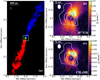 |
Fig. 1 Overview of the Ll448-mm system, as seen by ALMA. Panel a: overview of the region. The red and blue lobes of the jet are indicated by the SiO (8–7) peak intensity map. Green corresponds to the ~0.9 mm continuum. The beams of SiO (empty) and continuum (filled) are shown on the top left. Panel b: zoomed-in image of the H13CN (4–3) peak intensity map with continuum contours in white at [10, 30, 100]σcont with σcont = 0.25 mJy beam−1. Panel c: same as b, but for CH3OH (22,1,0—31,2,0). In panels b and c the peak of the continuum is indicated by a cross and the integrated intensity maps of the high-velocity bullets of SiO (65–75 km s−1) are shown in red and blue contours (at [10, 15, 20]σSiO,mom0 with σSiO,mom0 = 6 mJy beam−1 km s−1). |
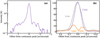 |
Fig. 2 Intensity cuts perpendicular to the jet axis, (a) Continuum intensity profile on larger scale, showing the bright central disk on top of an extended envelope pedestal, (b) Intensity profiles on disk scales of continuum (purple), CH3OH before continuum subtraction (gray), and CH3OH after continuum subtraction (orange), showing the artificial formation of a central hole surrounded by a faint ring. |
3.2 Infall, stellar mass, centrifugal radius, and accretion rate
The larger scale envelope is traced by H13CO+ for this source (van’t Hoff et al. 2022). Figure B.l presents the channel maps of H13CO+. Already in Fig. B.l some signs of rotation in the envelope are present, as well as infall (superposed blue and red emission at the same position). To investigate this further, Fig. presents its position-velocity (P–V) diagram over a cut perpendicular to the jet axis through the continuum peak. Figure 3 shows that the kinematics of H13CO+ along the disk major axis on scales 0.1–0.8″ = 30–240 au is well reproduced by a ballistic model of a rotating and infalling flattened envelope (see Sakai et al. 2014; Lee et al. 2017 for model details) with a central mass of ~0.4 ± 0.1 M⊙ (constrained by the infall pattern of blue plus red superposition at low V and large radii) and a constant deprojected specific angular momentum of lenv ≃ 130 ± 20 au km s−1 (constrained by the pure rotating pattern at radial velocities V > 2 km s−1), considering inclination angles ~30º–44º (see Sect. 3.1). In the rest of this work we consider two protostellar masses (M⋆) of 0.3 M⊙ and 0.5 M⊙ to cover the measured range of masses including the uncertainty1. Gaudel et al. (2020) found a similar value on the same scales, lenv ≃ 120 ± 20 au km s−1, despite their use of a much higher inclination of i = 70°. We checked that their measured V(R) agree very well with the brightest branches of our P–V cut in H13CO+. The fainter branches of opposite velocity sign (which signify infall) could not be retrieved with their method2. The neglect of infall motions thus increases the contribution of rotation to the V(R) curve, leading to a larger projected angular momentum lenv sin i. The use of i = 70° by Gaudel et al. (2020) to deproject, instead of i = 30°–44° here, has the opposite effect, leading to a deprojected lenv similar to ours.
The corresponding centrifugal barrier radius, , agrees with the dust disk radius (~23au; see Sect. 3.1), as also found for L1527 and HH212 (Sakai et al. 2014; Lee et al. 2017). The protostellar mass can be used to estimate the accretion rate onto the star, Ṁacc, assuming that the bolometric luminosity is dominated by the accretion luminosity, Lacc ≃ GṀ⋆Ṁacc/R⋆ (Hartmann et al. 1998). For Lacc = 9 L⊙, M⋆ = 0.3–0.5 M⊙, and taking the appropriate stellar radius for an accreting protostar of this mass, R⋆ = 3 R⊙ (Stahler 1988), we find Ṁacc ≃ (2–3) × 10−6 M⊙yr−1. This amounts to ten times the mass-flux of the high-velocity jet in Ll448-mm, inferred from [OI]63 µm maps (Nisini et al. 2015), a result fully consistent with the typical ejection-to-accretion ratio ≃10% observed in protostellar jets (see, e.g., Lee 2020).
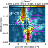 |
Fig. 3 P–V diagram of H13CO+ (4–3) perpendicular to the jet axis, averaged over a slit width of ~1 beam. The black contours show the [5, 8, 12]σ levels, where σ is given in Table 1. The magenta curves indicate an infalling rotating envelope model with lenv of 130 au km s−1, M⋆ = 0.4 M⊙, inclination angle of ί = 30° to the line of sight, and centrifugal barrier rc = 24 au. |
3.3 Rotating small-scale outflow
Moment 1 maps and transverse P–V diagrams of the selected small-scale outflow tracers (CH3OH, H13CN, and SO) are presented in Figs. 4 and 5, while their channel maps are presented in Fig. B.2. Of the three tracers, methanol exhibits the most compact emission. This is likely due to methanol mainly forming in prestellar ices and later sublimating close to the protostar at temperatures of ≳100 K (Minissale et al. 2022), while SO and HCN can efficiently form in the gas phase in disk winds (Panoglou et al. 2012; Gressel et al. 2020).
The transverse centroid gradient in the methanol Moment 1 map and the tilt in its transverse P–V cuts both show clear signatures of rotation in the same direction as the envelope. However, the emission is elongated along the jet axis, which is inconsistent with disk emission. Moreover, the Moment 1 map reveals a global velocity shift of ±0.5 km s−1 between the red (SE) and blue (NW) lobes, consistent with a slow outflowing motion. These results demonstrate that methanol emission in L1448-mm traces the base of the outflow and not the inner envelope or the rotating disk. This supports the proposal of Codella et al. (2018), who suggested that complex organics in HH 212 could be a part of the outflow, and revises the classical picture of hot corinos that trace the infalling envelope material (Ceccarelli 2004).
Belloche et al. (2020) argued that the emission size of complex organic molecules in L1448-mm can be marginally explained by a hot corino scenario (i.e., thermal desorption close to the protostar). This would agree with the prediction of 2D radiative transfer models of Nazari et al. (2022) for disk plus envelope structures including outflow cavities. They showed methanol emission along and outside the outflow cavity walls due to thermal desorption, with a similar size and flux to those observed here. However, whether the methanol emission inside of the outflow itself is due to thermal desorption or mechanical ice sputtering due to ion-neutral drift is unclear.
The H13CN emission also traces the base of the outflow, but extends farther away from the disk, up to a projected distance of ɀproj ~ 150 au. Its Moment 1 map, and the tilt at low velocity in transverse P–V cuts, again reveal clear rotation signatures consistent with the rotation direction of the envelope. In contrast with methanol, however, the P–V cuts in H13CN at small vertical distances ɀproj ≃ 30–60 au also trace faster gas closer to the jet axis, suggestive of an “onion-like” nested velocity structure inside the low-velocity rotating flow. At larger distance (ɀproj = 120 au), this faster component disappears and the P–V cut exhibits an empty ring-like morphology, pointing toward a thinner shell of outflowing gas, where the rotation signature (tilt) clearly persists. Such a ring-like structure has been observed previously in other disk wind candidates, such as HH30 and Orion Source I (Louvet et al. 2018; Hirota et al. 2017; López-Vázquez et al. 2020).
SO has previously been identified in HH 212 as a promising tracer of disk winds (Tabone et al. 2017). Here a comparison of the P–V cuts in Fig. 5 confirms that SO is tracing the same rotating small-scale outflow as H13CN. However, the emission appears less extended in the transverse direction and more complex compared with H13CN (e.g., the presence of both blue- and redshifted emission in the NW P–V cuts at ɀproj = 30–90 au).
This is likely due to a combination of chemical and optical depth effects, and to a larger contribution from jet bowshocks in SO. In the following we therefore focus on CH3OH and H13CN.
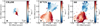 |
Fig. 4 Moment 1 (intensity-weighted velocity) maps of CH3OH (22,1,0−31,2,0), H13CN (4−3), and SO (89−78) demonstrating rotation in their low-velocity outflow component. The velocity ranges used to compute the maps are ±4, ±5, and ±8 km s−1 for CH3OH, H13CN, and SO, respectively, and a cut at ~3σ is made. The black cross in all panels indicates the continuum peak. |
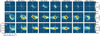 |
Fig. 5 Transverse P–V diagrams of CH3OH (22,1,0−31,2,0), H13CN (4−3), and SO (89−78) perpendicular to the jet axis, at projected offsets ɀproj ~ 30, 60, 90, and 120 au from the continuum peak, and averaged over a slit width of ~1 beam. Cuts through the red (resp. blue) lobe are labeled SE for southeast (resp. NW for northwest). The black solid curves show predictions for a thin shell model of rotating conical flow with a base radius of ~19 au, obtained by fitting the SE P–V cuts of CH3OH and H13CN (see green curves in Fig. A.2). The same model is overlaid in dashed lines on SE P–V cuts of SO for comparison. |
4 Evidence for an MHD disk wind
4.1 Wind morphology and kinematics
The rotation signatures in the outflow of L1448-mm, its small float radius, and its nested velocity structure (see Sect. 3.3) are strongly suggestive of an MHD disk wind. The shape of the P–V diagrams is well in line with the synthetic predictions of extended MHD disk winds, with faster gas launched closer to the protostar (Tabone et al. 2020). In order to more quantitatively test this claim, we analyzed the P–V diagrams of H13CN and CH3OH focusing on the redshifted lobe. The P–V cuts there are more dominated by the low-velocity rotating component than in the blueshifted lobe, and show a clearer ring pattern at ɀproj = 120 au, allowing for a more robust fitting of the outermost emitting layer.
We use a method independent from simulations of MHD disk winds to retrieve the spatio-kinematical structure of the outer outflow from the observed P–V diagrams. Our model assumes a thin axisymmetric rotating shell of gas to retrieve the flow shape r(ɀ), υϕ (rotational velocity), and υɀ (velocity along the axis). The transverse velocity υr can also be inferred assuming flow along the cone. The details of our method are explained in Appendix A (see also Louvet et al. 2018; Tabone et al. 2020; de Valon et al. 2022).
The black curves in Fig. 5 show the location of emission expected from the thin shell model at different projected distances from the protostar (ɀproj). We find that the morphology of the brightest features in the observed P–V diagrams closely match the thin shell model. Overall, the shape of the outflow is well fitted by a conical flow with a half-opening angle of i ≃ 13°, with its base at ~ 19 au from the central protostar. The observed P–V diagram of H13CN is notably well described at ɀproj = 120 au by a cone-like structure for which the base is traced by CH3OH emission. At ɀproj ≲ 60 au, the H13CN P–V cuts show additional emission closer to the jet axis and at higher velocity that is not reproduced by the model. At these locations, our thin shell model provides only the shape and kinematics of the outermost wind streamline emitting in this tracer.
We find that the retrieved axial velocity of the flow increases with distance, from υɀ ≃ 1 km s−1 at its base (traced by both methanol and H13CN) to about 4 km s−1 at a deprojected distance of ɀ ≃ 260 au (traced only by H13CN; Fig. A.2). The rotation velocity is found to be constant and about υϕ ≃ 4 ± 2 km s−1. Given the large uncertainties on υϕ, we infer a tentative increase in the specific angular momentum with distance.
4.2 Wind launching point and magnetic lever arm parameter
The retrieved kinematics of the wind allows us to infer the launching point of the wind r0 using the Anderson relation (Eq. (4) in Anderson et al. 2003), given by
 (4)
(4)
This relation is valid at any point in a cold, steady, axisymmetric MHD disk wind where gravitational potential can be neglected, and directly follows from the conservation of energy and angular momentum (Anderson et al. 2003). In Eq. (4), r is the radial distance from the jet axis, υϕ the rotational velocity, υpol the poloidal velocity, and Ω0 is the orbital frequency at the launching radius  .
.
Our results are summarized in Fig. 6 where we plot our CH3OH and H13CN measurements at various ɀproj (from Fig. A.2) on top of the predicted relation between rυϕ and  from Eq. (4), for various values of r0 (solid curves). We considered a stellar mass, M★, in the range 0.3–0.5 M⊙, as inferred from envelope infall kinematics (Sect. 3.2). Figure 6 assumes a protostellar mass of 0.5 M⊙ and Fig. B.3 shows the same diagram assuming a smaller M★ = 0.3 M⊙. The conclusions are unchanged. Even if the disk mass was as high as 0.1 M⊙ (the upper limit estimated in Sect. 3.1), and the protostellar mass as low as 0.2 M⊙, the inferred launch radii would only increase by ~1–2 au.
Based on Figs. 6 and B.3 we find that the launching radii inferred at the various distances zproj roughly agree with each other at  au. Here 10 au is approximately the average of the two medians of r0 for M★ of 0.3 M⊙ and 0.5 M⊙. The uncertainties on this value are based on the range that is seen in the data points (including their error bars) and up to the radii below the disk radius of 23 au. We note that the inferred launching radius corresponds to the outermost emitting streamline of the wind since we retrieved the wind kinematics from the outer boundary of the outflow in P–V cuts. This is consistent with the determined dust disk radius of ~23 au (Sect. 3.1) and the extrapolated float radius of the cone-like shape of the outflow from our best-fit model to P–V diagrams of Fig. 5 (~19 au; see Appendix A). It excludes an X-wind origin, with launching radius ≲0.1 au. Including the gravitational potential term (Φ𝑔 in Eq. (3) of Anderson et al. 2003) would only affect the launching radius by ~1–5 au, which is within the uncertainties of our r0 estimates. We also find a tentative increase in the wind launching radius from r0 ≃ 10 au to r0 ≃ 20 au moving farther away from the disk. One possibility is that the wind at large distances is slightly perturbed and compressed by jet bow-shocks (Tabone et al. 2018), highlighting outer streamlines that remained unseen at the base of the outflow due to insufficient excitation or chemical abundance of HCN. A perturbation by the jet would also explain why the outflow is resolved as a relatively thin shell at large distances from the disk (ɀp ≳ 90), while it would be constantly refilled by the disk wind at low altitudes (Tabone et al. 2018).
A lower limit to the magnetic lever arm parameter can also be inferred as  (Ferreira et al. 2006). Combining this expression with Eq. (4) yields
  , and hence
 (5)
(5)
This predicted inverse relation between rυϕ and υtot is plotted as dashed curves in Figs. 6 and B.3 for various values of λϕ. A comparison with the observed data points in L1448-mm indicates relatively low values of λϕ ≃ 1.7–2.3, similar to those found for other rotating MHD disk wind candidates, such as HH212 (≲5; Tabone et al. 2017), HH30 (≃1.6; Louvet et al. 2018), and DG Tau B (≃1.6; de Valon et al. 2022). We note that λϕ is different from λBP (Blandford & Payne 1982; Tabone et al. 2020). The latter measures the total specific angular momentum carried away by the wind which includes the magnetic torsion, while the former only measures the specific angular momentum for the matter rotation and cannot be higher than λBP (Ferreira et al. 2006). We take λϕ ≃ 1 .7, consistent with the non-perturbed, inner data points in Figs. 6 and B.3, and thus a lower limit on λBP of 1.7. This low value of λBP is typically predicted for non-ideal MHD disk wind models with a relatively weak magnetization of β ≃ 103–104 in the disk midplane, where β is the thermal-to-magnetic pressure ratio (Lesur 2021). The corresponding disk surface density at 10 au is Σ ≃ 100–600 g cm−2, where we used Eq. (17) of Lesur (2021) with M★ = 0.4 ± 0.1 M⊙ and a wind-driven disk accretion rate Ṁacc ≃ (2–3) × 10−6 M⊙ yr−1 (see Sect. 3.2). Combined with the measured disk radius of 23 au, it translates into a disk mass  , fully consistent with our independent estimate from dust continuum (see Sect. 3.1).
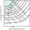 |
Fig. 6 Diagnostic diagram of MHD disk-wind launch point and magnetic lever arm, updated from Ferreira et al. (2006) showing specific angular momentum as a function of the total gas velocity. The data points at different altitudes from Fig. A.2 are shown in blue (H13CN) and pink (CH3OH), where a protostellar mass of 0.5 M⊙ was adopted. The black grid in the background shows the relation between these two quantities predicted when gravitational potential is negligible, for different values of the wind launching radius r0 (solid curves, Eq. (4)) and magnetic lever arm parameter λϕ (dashed curves, Eq. (5)). In contrast to the first version of this diagram, introduced in Ferreira et al. (2006), the x-axis here plots the total gas velocity instead of υpol, since the measured υϕ is of the same order as υpol. The region with r0 above the dust disk radius of 23 au is hatched in green. |
4.3 Wind mass-flux
Here we compare the wind ejection rate with the disk accretion rate to answer whether the wind can effectively drive accretion. The wind mass-loss rate was calculated by
 (6)
(6)
where mp is the proton mass, υɀ is taken as 2.5 km s−1 at a ɀproj of 60 au (see Fig. A.2), and the factor 1.4 is added to take into account the helium mass. The column density of HCN, NHCN, was calculated from that of H13CN using the CASSIS spectral analysis tool (Vastel et al. 2015) by assuming a 12C/13C ratio of 70 (Milam et al. 2005). The H13CN spectrum was extracted in a rectangular aperture perpendicular to the jet axis with a length dr = 2″ that encompasses all of the emission in the lateral direction to the jet axis, and a width of approximately one beam (0.1″). It was centered at 60 au from the continuum peak in the SE side. We note that because the H13CN line profile is asymmetric, we fitted two Gaussian profiles to find the column density using CASSIS. In this process, an excitation temperature of 100 K (Belloche et al. 2020) was assumed, leading to an aperture-averaged column density of  cm−2, and aperture-averaged line optical depth in each component ≲0.1. At ɀproj = 60 au, the flow width of ~0.4″ fills 1/5 of the aperture length (2″), and hence the true line optical depth is ≲0.5, and the optically thin assumption remains valid. The abundance of HCN with respect to the total hydrogen number density nH, XHCN, is assumed as 10−7 based on the measured column density ratios of HCN/CO in outflows from observations of Tafalla et al. (2010) and an assumed abundance of 10−4 for CO (e.g., Pineda et al. 2008). We note that XHCN is relatively uncertain in MHD wind models and could have variations of approximately one order of magnitude (e.g., Gressel et al. 2020), but 10−7 seems to be a good nominal value in observed proto-stellar outflows with smaller variations from source to source (a factor of ~3; Tafalla et al. 2010). From our H13CN observations, we estimate a mass-loss rate in the redshifted wind of ṀDW ~ 4 × 10⁻⁶ M⊙ yr−1. Doubling to account for the blue lobe, the total mass-flux (ṀDW,total) is ~2.5–4 times larger than the accretion rate found in Sect. 3.2.
The question arises of whether this wind could actually drive disk accretion at the estimated rate of Ṁacc ≃ (2–3) × 10−6 M⊙ yr−1. Assuming that all the angular momentum required to drive disk accretion is removed by the wind, Tabone et al. (2020) showed that the ratio of wind mass loss rate to disk accretion rate has to be (also see Pascucci et al. 2023)
 (7)
(7)
where rin and rout are the inner and outer launch radii of the wind. In Eq. (7) the lower the λBP, the larger the fM, which means more mass is required to be launched in the wind to drive disk accretion. Similarly, for a larger wind launching region, more angular momentum needs to be extracted to advect gas from rout to rin, increasing the mass-loss rate. The onion-like velocity structure seen in H13CN suggests that the wind launch radius extends down to a much smaller radius than 10–20 au. The inner launch radius of the flow traced by H13CN can be roughly estimated from the maximum projected velocity ~12 km s−1. Assuming that the inner streamline has λϕ ≃ 1 .7, consistent with our non-perturbed inner data points in Figs. 6 and B.3, and that the rotation velocity is similar to the axial velocity, as found for the outer streamline, we find from the Anderson relation that rin ≃ 1 au. Using the derived values rin = 1 au, rout = 10 au and a lower limit on λBP of 1.7 similar to λϕ, we find ƒM ~ 4, in agreement with the observationally derived mass-flux. We conclude that the total angular momentum carried away by the wind could be sufficient to drive disk accretion in the bulk of the disk.
5 Concluding remarks
In this paper we presented high angular resolution (≲0.1″ ; ~30 au) and high-sensitivity ALMA observations of the L1448 protostellar system. Various components of the system (i.e., disk, inner envelope, and rotating outflow) are resolved for the first time. We attribute the rotating emission from CH3OH and H13CN at the base of the outflow to an MHD disk wind and suggest these two molecules as new tracers of an MHD disk wind for future observations. These two molecules are complementary to the previously identified disk wind tracers such as SO because they are less contaminated by jet bowshocks and SO is more affected by chemistry and optical depth. Moreover, it is debated whether methanol, or more generally COMs, trace the inner warm envelope as sublimated from the ices or if their emission structure is affected by shocks, disk winds, and the presence of a disk. Here we find that methanol traces a rotating MHD disk wind candidate. Overall, our analysis opens new avenues to study the chemistry of disk-winds. Notably, understanding the formation, survival, and excitation of molecules such as SO, HCN, or methanol in those winds will be crucial to constrain the physics of disk-winds and access the composition of disks at the launching points of these winds.
We estimated the outer wind launch radius to be about ~ 10–20 au. The onion-like structure of the flow indicates that the launching zone of the wind is extended down to ~1 au. The magnetic lever arm parameter is relatively low ~1.7, in line with MHD disk wind models from weakly magnetized disks (β ≃ 103–104). The mass-flux appears sufficient to drive disk accretion at the current rate. Detailed comparisons with MHD disk wind model predictions, and with alternative envelope entrainment models (e.g., Rabenanahary et al. 2022) are now required to obtain more robust constraints and definitely test the MHD interpretation.
Acknowledgements
We thank the referee for their constructive comments. We thank N.T. Kurtovic for the helpful discussions. Astrochemistry in Leiden is supported by EU A-ERC grant 101019751 MOLDISK, NOVA, and by the NWO grant 618.000.001. Support by the Danish National Research Foundation through the Center of Excellence “InterCat” (Grant agreement no.: DNRF150) is also acknowledged. B.T. and S.C. acknowledge support from the Programme National “Physique et Chimie du Milieu Interstellaire” (PCMI) of CNRS/INSU with INC/INP and co-funded by CNES. L.P. and C.C. acknowledge the project PRIN MUR 2022 FOSSILS (Chemical origins: linking the fossil composition of the Solar System with the chemistry of protoplanetary disks, Prot. 2022JC2Y93) and the INAF Mini-Grant 2022 “Chemical Origins” (PI: L. Podio). Ł.T. acknowledges support from the ESO Fellowship Program. This paper makes use of the following ALMA data: ADS/JAO.ALMA#2021.1.01578.S. ALMA is a partnership of ESO (representing its member states), NSF (USA) and NINS (Japan), together with NRC (Canada), MOST and ASIAA (Taiwan), and KASI (Republic of Korea), in cooperation with the Republic of Chile. The Joint ALMA Observatory is operated by ESO, AUI/NRAO and NAOJ. The National Radio Astronomy Observatory is a facility of the National Science Foundation operated under cooperative agreement by Associated Universities, Inc.
Appendix A A simple model for the outflow shape and kinematics
Here we explain a method to retrieve the velocities υϕ, υr, υɀ, and the shape of the outermost emitting layer of the outflow. This emitting layer may not correspond to a single streamline, due to chemical and excitation gradients. This method is applied to the redshifted lobe in Sect. 4. We show a sketch of the outflow geometry and define quantities used in the following in Fig. A.1. We assume that the outflow is axisymmetric. The outermost layer of the outflow can be divided into rings at different heights ɀ from the protostar (see light green ring in Fig. A.1). The velocity of this ring in the cylindrical coordinate system defined by the outflow axis is described by the rotation velocity υϕ, the radial velocity υr, and the axial velocity υɀ. We define the inclination angle i as the angle between the blue lobe and the line of sight with i = 0 for face-on and i = π/2 for edge-on configuration. In this convention, υɀ is positive in the blueshifted lobe and negative in the redshifted lobe, and the blueshifted lobe is mostly projected in the ɀproj > 0 region of the sky. Based on the geometry presented in Fig. A.1 a gas parcel located at a position (r, ɀ, ϕ) along the ring is projected on the plane of the sky at
 (A.1)
(A.1)
 (A.2)
(A.2)
and has a projection velocity (also often called radial velocity)
 (A.3)
(A.3)
where subscript proj indicates projected, and where positive velocities stand for redshifted material.
Our aim is to retrieve the outer radius of the flow r and the three velocity components as a function of ɀ from the transverse P–V diagrams. The challenge comes from the fact that even at high angular resolution, a transverse P–V diagram contains the emission from a collection of gas parcels located at different positions (r, ɀ, ϕ). However, at given ɀproj the maximum projected radii beyond which no emission is detected in the P–V diagram, denoted as rproj,1 (> 0) and rproj,2 (< 0), correspond to gas parcels located at ϕ = −90° and +90°, respectively, r = rproj,1 ≃ −rproj,2 and ɀ = ɀproj/ sin i (see the two orange crosses in Fig. A.1). The shape of the outer layer of the outflow r(ɀ) can therefore be directly inferred from the measurement of rproj,1 and rproj,2 at different distances ɀproj as
 (A.4)
(A.4)
Regarding the kinematics of the outflow, we note that the gas parcels emitting at rproj,1 and rproj,2 have projected velocities of υproj,1 = − υɀcos i − υϕ sin i and υproj,2 = − υɀcos i + υϕ sin i. Therefore, the velocities found in the transverse P–V diagram at rproj,1 and rproj,2 give the rotation and axial velocity at a distance ɀ = ɀproj/ sin i of
 (A.5)
(A.5)
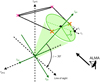 |
Fig. A.1 Sketch of the outflow orientation relative to the plane of the sky. The black dashed lines (sky plane) are perpendicular to each other. The green solid lines (jet plane) are also perpendicular to each other. The orange crosses on the ring around the outflow walls correspond to the pink crosses on the solid circle, which is the projection of the green ring onto the sky plane. Orange crosses are located at ϕ = ±90°. |
P–V measurements
We report in Table A.1 the values of rproj,1/2 and υproj,1/2 measured for H13CN and CH3OH at various ɀproj. The shape of the outflow, υϕ, and υɀ were then calculated from Eqs. (A.4) and (A.5). Finally, we find υr by assuming that the poloidal velocity is tangential to the flow shape. Figure A.2 presents the measured values of υɀ, υϕ, and rυϕ as a function of ɀ.
In order to check the method, we computed the location of the emission in each P–V diagram (see black lines in Fig. 5), accounting for the contribution of all the gas parcels and not only those at ϕ = ±90°. In order to do so, one needs to prescribe r, υϕ, υɀ, and υr as function of ɀ. These relations are obtained by fitting the shape of the outflow by a cone and the υɀ by a linear function of ɀ. We assume υϕ to be constant and equal to +3.5 km s−1. During this process, we played with the various parameters to find the best-fitting ring-like structure for the P–V diagrams. The best fit to the P–V diagrams in Fig. 5 results in a relation between r and ɀ, and υɀ and ɀ of (ɀ/1 au) = ±4.3(r/1 au) + 80 and (υɀ/1 km s−1) = 0.018(z/1 au) − 0.1, respectively (green curves in Fig. A.2).
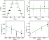 |
Fig. A.2 Retrieved shape and kinematics of the wind outermost emitting layer in the red lobe. Radius r (top left), velocities υϕ (top right) and υɀ (bottom right), and specific angular momentum r × υϕ (bottom left) are shown as a function of deprojected altitude ɀ. The data points with error bars represent values for CH3OH (pink) and H13CN (black), derived from the P–V measurements in Table A.1 and deprojected by an inclination i = 30°. The values of r × υϕ are computed using the average flow radius between the two edges. The green lines show our simple conical model that best fit the P–V diagrams in Fig. 5, assuming a flow along the cone walls. |
Appendix B Additional plots
Figure B.1 presents the channel maps of H13CO+ in the L1448-mm system. Figure B.2 presents the channel maps of CH3OH (22,1,0 − 31,2,0), H13CN (4-3), and SO (89 − 78) to demonstrate the rotation in their outflow emission. Figure B.3 is the same as Fig. 6, but for a protostar with a mass of 0.3 M⊙.
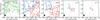 |
Fig. B.1 Channel maps of H13CO+ 4-3. To create this image the cube was re-binned in the spectral axis by a factor of two to increase the S/N. The contours are at levels [6, 9, 14]σ, where σ of this re-binned cube is equal to 1.8 mJy beam−1. The red and blue contours correspond to positive and negative velocities respectively, expressed in km s−1 with respect to the adopted systemic velocity Vsys (= 5.3 km s−1 in the LSR frame). The peak of the continuum is indicated by a cross and the jet axis by a dotted line. |
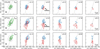 |
Fig. B.2 Channel maps of CH3OH (22,1,0 − 31,2,0), H13CN (4-3), and SO (89 − 78) in the inner ~l.5″ region. The continuum contours are shown in gray and they are set at [10, 30, 100]σcont with σcont = 0.25 mJy beam−1. The peak of the continuum is indicated by a cross. The red and blue contours correspond to positive and negative velocities respectively, expressed in km s−1 with respect to the adopted systemic velocity Vsys (= 5.3 km s−1 in the LSR frame). The contour levels are set at [7, 13, 20]σ for CH3OH and H13CN, and [6, 10, 15]σ for SO with σ given in Table 1. The molecules shown here show rotation signatures at |V| < 3 km s−1 in the inner regions or in the outflow emission. |
References
- Anderl, S., Maret, S., Cabrit, S., et al. 2016, A&A, 591, A3 [NASA ADS] [CrossRef] [EDP Sciences] [Google Scholar]
- Anderson, J. M., Li, Z.-Y., Krasnopolsky, R., & Blandford, R. D. 2003, ApJ, 590, L107 [Google Scholar]
- André, P., Men’shchikov, A., Bontemps, S., et al. 2010, A&A, 518, L102 [NASA ADS] [CrossRef] [EDP Sciences] [Google Scholar]
- Bachiller, R., Cernicharo, J., Martin-Pintado, J., Tafalla, M., &Lazareff, B. 1990, A&A, 231, 174 [NASA ADS] [Google Scholar]
- Bachiller, R., Martin-Pintado, J., & Fuente, A. 1991, A&A, 243, L21 [NASA ADS] [Google Scholar]
- Bachiller, R., Guilloteau, S., Dutrey, A., Planesas, P., & Martin-Pintado, J. 1995, A&A, 299, 857 [NASA ADS] [Google Scholar]
- Bai, X.-N., & Stone, J. M. 2013, ApJ, 769, 76 [Google Scholar]
- Balbus, S. A., & Hawley, J. F. 1998, Rev. Mod. Phys., 70, 1 [Google Scholar]
- Belloche, A., Maury, A. J., Maret, S., et al. 2020, A&A, 635, A198 [NASA ADS] [CrossRef] [EDP Sciences] [Google Scholar]
- Bjerkeli, P., van der Wiel, M. H. D., Harsono, D., Ramsey, J. P., & Jørgensen, J. K. 2016, Nature, 540, 406 [Google Scholar]
- Blandford, R. D., & Payne, D. G. 1982, MNRAS, 199, 883 [CrossRef] [Google Scholar]
- Boehler, Y., Weaver, E., Isella, A., et al. 2017, ApJ, 840, 60 [Google Scholar]
- Ceccarelli, C. 2004, ASP Conf. Ser., 323, 195 [Google Scholar]
- Ceccarelli, C., Codella, C., Balucani, N., et al. 2022, arXiv e-prints [arXiv:2206.13270] [Google Scholar]
- Codella, C., Bianchi, E., Tabone, B., et al. 2018, A&A, 617, A10 [NASA ADS] [CrossRef] [EDP Sciences] [Google Scholar]
- De Simone, M., Ceccarelli, C., Codella, C., et al. 2020, ApJ, 896, L3 [NASA ADS] [CrossRef] [Google Scholar]
- de Valon, A., Dougados, C., Cabrit, S., et al. 2020, A&A, 634, L12 [NASA ADS] [CrossRef] [EDP Sciences] [Google Scholar]
- de Valon, A., Dougados, C., Cabrit, S., et al. 2022, A&A, 668, A78 [NASA ADS] [CrossRef] [EDP Sciences] [Google Scholar]
- Ferreira, J. 1997, A&A, 319, 340 [Google Scholar]
- Ferreira, J., Dougados, C., & Cabrit, S. 2006, A&A, 453, 785 [NASA ADS] [CrossRef] [EDP Sciences] [Google Scholar]
- Ferrero, S., Zamirri, L., Ceccarelli, C., et al. 2020, ApJ, 904, 11 [NASA ADS] [CrossRef] [Google Scholar]
- Gaudel, M., Maury, A. J., Belloche, A., et al. 2020, A&A, 637, A92 [NASA ADS] [CrossRef] [EDP Sciences] [Google Scholar]
- Girart, J. M., & Acord, J. M. P. 2001, ApJ, 552, L63 [CrossRef] [Google Scholar]
- Gressel, O., Ramsey, J. P., Brinch, C., et al. 2020, ApJ, 896, 126 [Google Scholar]
- Hartmann, L., Calvet, N., Gullbring, E., & D’Alessio, P. 1998, ApJ, 495, 385 [Google Scholar]
- Hartmann, L., Herczeg, G., & Calvet, N. 2016, ARA&A, 54, 135 [Google Scholar]
- Hildebrand, R. H. 1983, QJRAS, 24, 267 [NASA ADS] [Google Scholar]
- Hirano, N., Ho, P. P. T., Liu, S.-Y., et al. 2010, ApJ, 717, 58 [NASA ADS] [CrossRef] [Google Scholar]
- Hirota, T., Machida, M. N., Matsushita, Y., et al. 2017, Nat. Astron., 1, 0146 [Google Scholar]
- Launhardt, R., Pavlyuchenkov, Y., Gueth, F., et al. 2009, A&A, 494, 147 [NASA ADS] [CrossRef] [EDP Sciences] [Google Scholar]
- Lee, C.-F. 2020, A&A Rev., 28, 1 [NASA ADS] [CrossRef] [Google Scholar]
- Lee, C.-F., Li, Z.-Y., Ho, P. T. P., et al. 2017, ApJ, 843, 27 [NASA ADS] [CrossRef] [Google Scholar]
- Lee, C.-F., Li, Z.-Y., Codella, C., et al. 2018, ApJ, 856, 14 [CrossRef] [Google Scholar]
- Lesur, G. R. J. 2021, A&A, 650, A35 [NASA ADS] [CrossRef] [EDP Sciences] [Google Scholar]
- Lesur, G., Flock, M., Ercolano, B., et al. 2023, ASP Conf. Ser., 534, 465 [NASA ADS] [Google Scholar]
- López-Vázquez, J. A., Zapata, L. A., Lizano, S., & Cantó, J. 2020, ApJ, 904, 158 [CrossRef] [Google Scholar]
- Louvet, F., Dougados, C., Cabrit, S., et al. 2018, A&A, 618, A120 [NASA ADS] [CrossRef] [EDP Sciences] [Google Scholar]
- Lynden-Bell, D., & Pringle, J. E. 1974, MNRAS, 168, 603 [Google Scholar]
- Manara, C. F., Ansdell, M., Rosotti, G. P., et al. 2023, ASP Conf. Ser., 534, 539 [NASA ADS] [Google Scholar]
- Maury, A. J., André, P., Testi, L., et al. 2019, A&A, 621, A76 [NASA ADS] [CrossRef] [EDP Sciences] [Google Scholar]
- McMullin, J. P., Waters, B., Schiebel, D., Young, W., & Golap, K. 2007, ASP Conf. Ser., 376, 127 [Google Scholar]
- Milam, S. N., Savage, C., Brewster, M. A., Ziurys, L. M., & Wyckoff, S. 2005, ApJ, 634, 1126 [Google Scholar]
- Minissale, M., Aikawa, Y., Bergin, E., et al. 2022, ACS Earth Space Chem., 6, 597 [NASA ADS] [CrossRef] [Google Scholar]
- Müller, H. S. P., Thorwirth, S., Roth, D. A., & Winnewisser, G. 2001, A&A, 370, L49 [Google Scholar]
- Müller, H. S. P., Schlöder, F., Stutzki, J., & Winnewisser, G. 2005, J. Mol. Struc., 742, 215 [Google Scholar]
- Nazari, P., Tabone, B., Rosotti, G. P., et al. 2022, A&A, 663, A58 [NASA ADS] [CrossRef] [EDP Sciences] [Google Scholar]
- Nisini, B., Santangelo, G., Giannini, T., et al. 2015, ApJ, 801, 121 [NASA ADS] [CrossRef] [Google Scholar]
- Ortiz-León, G. N., Loinard, L., Dzib, S. A., et al. 2018, ApJ, 865, 73 [Google Scholar]
- Ossenkopf, V., & Henning, T. 1994, A&A, 291, 943 [NASA ADS] [Google Scholar]
- Panoglou, D., Cabrit, S., Pineau Des Forêts, G., et al. 2012, A&A, 538, A2 [CrossRef] [EDP Sciences] [Google Scholar]
- Pascucci, I., Cabrit, S., Edwards, S., et al. 2023, ASP Conf. Ser., 534, 567 [NASA ADS] [Google Scholar]
- Pineda, J. E., Caselli, P., & Goodman, A. A. 2008, ApJ, 679, 481 [Google Scholar]
- Podio, L., Tabone, B., Codella, C., et al. 2021, A&A, 648, A45 [NASA ADS] [CrossRef] [EDP Sciences] [Google Scholar]
- Rabenanahary, M., Cabrit, S., Meliani, Z., & Pineau des Forêts, G. 2022, A&A, 664, A118 [NASA ADS] [CrossRef] [EDP Sciences] [Google Scholar]
- Rosotti, G. P., Ilee, J. D., Facchini, S., et al. 2021, MNRAS, 501, 3427 [Google Scholar]
- Sakai, N., Sakai, T., Hirota, T., et al. 2014, Nature, 507, 78 [Google Scholar]
- Shakura, N. I., & Sunyaev, R. A. 1973, A&A, 24, 337 [NASA ADS] [Google Scholar]
- Stahler, S. W. 1988, ApJ, 332, 804 [NASA ADS] [CrossRef] [Google Scholar]
- Tabone, B., Cabrit, S., Bianchi, E., et al. 2017, A&A, 607, L6 [NASA ADS] [CrossRef] [EDP Sciences] [Google Scholar]
- Tabone, B., Raga, A., Cabrit, S., & Pineau des Forêts, G. 2018, A&A, 614, A119 [CrossRef] [EDP Sciences] [Google Scholar]
- Tabone, B., Cabrit, S., Pineau des Forêts, G., et al. 2020, A&A, 640, A82 [CrossRef] [EDP Sciences] [Google Scholar]
- Tabone, B., Rosotti, G. P., Lodato, G., et al. 2022, MNRAS, 512, L74 [NASA ADS] [CrossRef] [Google Scholar]
- Tafalla, M., Santiago-García, J., Hacar, A., & Bachiller, R. 2010, A&A, 522, A91 [CrossRef] [EDP Sciences] [Google Scholar]
- Tobin, J. J., Looney, L. W., Li, Z.-Y., et al. 2016, ApJ, 818, 73 [CrossRef] [Google Scholar]
- Toledano-Juárez, I., de la Fuente, E., Trinidad, M. A., Tafoya, D., & Nigoche-Netro, A. 2023, MNRAS, 522, 1591 [CrossRef] [Google Scholar]
- Tomida, K., Tomisaka, K., Matsumoto, T., et al. 2010, ApJ, 714, L58 [NASA ADS] [CrossRef] [Google Scholar]
- Tychoniec, L., Tobin, J. J., Karska, A., et al. 2018, ApJS, 238, 19 [NASA ADS] [CrossRef] [Google Scholar]
- Tychoniec, L., van Dishoeck, E. F., van’t Hoff, M. L. R., et al. 2021, A&A, 655, A65 [NASA ADS] [CrossRef] [EDP Sciences] [Google Scholar]
- van Gelder, M. L., Nazari, P., Tabone, B., et al. 2022, A&A, 662, A67 [NASA ADS] [CrossRef] [EDP Sciences] [Google Scholar]
- van’t Hoff, M. L. R., Harsono, D., van Gelder, M. L., et al. 2022, ApJ, 924, 5 [CrossRef] [Google Scholar]
- Vastel, C., Bottinelli, S., Caux, E., Glorian, J. M., & Boiziot, M. 2015, in SF2A-2015: Proceedings of the Annual meeting of the French Society of Astronomy and Astrophysics, 313 [Google Scholar]
- Weaver, E., Isella, A., & Boehler, Y. 2018, ApJ, 853, 113 [Google Scholar]
- Yoshida, T., Hsieh, T.-H., Hirano, N., & Aso, Y. 2021, ApJ, 906, 112 [CrossRef] [Google Scholar]
The effect of a disk mass of 0.1 M⊙ is discussed in Sect. 4.2.
They fitted a single position centroid in each velocity channel (at radii <1″), or a single velocity centroid (Moment 1) at each position (at radii 1–3.5″).
All Tables
All Figures
|
Fig. 1 Overview of the Ll448-mm system, as seen by ALMA. Panel a: overview of the region. The red and blue lobes of the jet are indicated by the SiO (8–7) peak intensity map. Green corresponds to the ~0.9 mm continuum. The beams of SiO (empty) and continuum (filled) are shown on the top left. Panel b: zoomed-in image of the H13CN (4–3) peak intensity map with continuum contours in white at [10, 30, 100]σcont with σcont = 0.25 mJy beam−1. Panel c: same as b, but for CH3OH (22,1,0—31,2,0). In panels b and c the peak of the continuum is indicated by a cross and the integrated intensity maps of the high-velocity bullets of SiO (65–75 km s−1) are shown in red and blue contours (at [10, 15, 20]σSiO,mom0 with σSiO,mom0 = 6 mJy beam−1 km s−1). |
| In the text | |
|
Fig. 2 Intensity cuts perpendicular to the jet axis, (a) Continuum intensity profile on larger scale, showing the bright central disk on top of an extended envelope pedestal, (b) Intensity profiles on disk scales of continuum (purple), CH3OH before continuum subtraction (gray), and CH3OH after continuum subtraction (orange), showing the artificial formation of a central hole surrounded by a faint ring. |
| In the text | |
|
Fig. 3 P–V diagram of H13CO+ (4–3) perpendicular to the jet axis, averaged over a slit width of ~1 beam. The black contours show the [5, 8, 12]σ levels, where σ is given in Table 1. The magenta curves indicate an infalling rotating envelope model with lenv of 130 au km s−1, M⋆ = 0.4 M⊙, inclination angle of ί = 30° to the line of sight, and centrifugal barrier rc = 24 au. |
| In the text | |
|
Fig. 4 Moment 1 (intensity-weighted velocity) maps of CH3OH (22,1,0−31,2,0), H13CN (4−3), and SO (89−78) demonstrating rotation in their low-velocity outflow component. The velocity ranges used to compute the maps are ±4, ±5, and ±8 km s−1 for CH3OH, H13CN, and SO, respectively, and a cut at ~3σ is made. The black cross in all panels indicates the continuum peak. |
| In the text | |
|
Fig. 5 Transverse P–V diagrams of CH3OH (22,1,0−31,2,0), H13CN (4−3), and SO (89−78) perpendicular to the jet axis, at projected offsets ɀproj ~ 30, 60, 90, and 120 au from the continuum peak, and averaged over a slit width of ~1 beam. Cuts through the red (resp. blue) lobe are labeled SE for southeast (resp. NW for northwest). The black solid curves show predictions for a thin shell model of rotating conical flow with a base radius of ~19 au, obtained by fitting the SE P–V cuts of CH3OH and H13CN (see green curves in Fig. A.2). The same model is overlaid in dashed lines on SE P–V cuts of SO for comparison. |
| In the text | |
|
Fig. 6 Diagnostic diagram of MHD disk-wind launch point and magnetic lever arm, updated from Ferreira et al. (2006) showing specific angular momentum as a function of the total gas velocity. The data points at different altitudes from Fig. A.2 are shown in blue (H13CN) and pink (CH3OH), where a protostellar mass of 0.5 M⊙ was adopted. The black grid in the background shows the relation between these two quantities predicted when gravitational potential is negligible, for different values of the wind launching radius r0 (solid curves, Eq. (4)) and magnetic lever arm parameter λϕ (dashed curves, Eq. (5)). In contrast to the first version of this diagram, introduced in Ferreira et al. (2006), the x-axis here plots the total gas velocity instead of υpol, since the measured υϕ is of the same order as υpol. The region with r0 above the dust disk radius of 23 au is hatched in green. |
| In the text | |
|
Fig. A.1 Sketch of the outflow orientation relative to the plane of the sky. The black dashed lines (sky plane) are perpendicular to each other. The green solid lines (jet plane) are also perpendicular to each other. The orange crosses on the ring around the outflow walls correspond to the pink crosses on the solid circle, which is the projection of the green ring onto the sky plane. Orange crosses are located at ϕ = ±90°. |
| In the text | |
|
Fig. A.2 Retrieved shape and kinematics of the wind outermost emitting layer in the red lobe. Radius r (top left), velocities υϕ (top right) and υɀ (bottom right), and specific angular momentum r × υϕ (bottom left) are shown as a function of deprojected altitude ɀ. The data points with error bars represent values for CH3OH (pink) and H13CN (black), derived from the P–V measurements in Table A.1 and deprojected by an inclination i = 30°. The values of r × υϕ are computed using the average flow radius between the two edges. The green lines show our simple conical model that best fit the P–V diagrams in Fig. 5, assuming a flow along the cone walls. |
| In the text | |
|
Fig. B.1 Channel maps of H13CO+ 4-3. To create this image the cube was re-binned in the spectral axis by a factor of two to increase the S/N. The contours are at levels [6, 9, 14]σ, where σ of this re-binned cube is equal to 1.8 mJy beam−1. The red and blue contours correspond to positive and negative velocities respectively, expressed in km s−1 with respect to the adopted systemic velocity Vsys (= 5.3 km s−1 in the LSR frame). The peak of the continuum is indicated by a cross and the jet axis by a dotted line. |
| In the text | |
|
Fig. B.2 Channel maps of CH3OH (22,1,0 − 31,2,0), H13CN (4-3), and SO (89 − 78) in the inner ~l.5″ region. The continuum contours are shown in gray and they are set at [10, 30, 100]σcont with σcont = 0.25 mJy beam−1. The peak of the continuum is indicated by a cross. The red and blue contours correspond to positive and negative velocities respectively, expressed in km s−1 with respect to the adopted systemic velocity Vsys (= 5.3 km s−1 in the LSR frame). The contour levels are set at [7, 13, 20]σ for CH3OH and H13CN, and [6, 10, 15]σ for SO with σ given in Table 1. The molecules shown here show rotation signatures at |V| < 3 km s−1 in the inner regions or in the outflow emission. |
| In the text | |
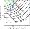 |
Fig. B.3 Same as Fig. 6, but assuming a protostellar mass of 0.3 M⊙. |
| In the text | |
Current usage metrics show cumulative count of Article Views (full-text article views including HTML views, PDF and ePub downloads, according to the available data) and Abstracts Views on Vision4Press platform.
Data correspond to usage on the plateform after 2015. The current usage metrics is available 48-96 hours after online publication and is updated daily on week days.
Initial download of the metrics may take a while.