| Issue |
A&A
Volume 639, July 2020
|
|
|---|---|---|
| Article Number | A87 | |
| Number of page(s) | 25 | |
| Section | Interstellar and circumstellar matter | |
| DOI | https://doi.org/10.1051/0004-6361/202037758 | |
| Published online | 13 July 2020 | |
Complex organic molecules in low-mass protostars on Solar System scales
I. Oxygen-bearing species★
1
Leiden Observatory, Leiden University,
PO Box 9513,
2300 RA
Leiden, The Netherlands
e-mail: This email address is being protected from spambots. You need JavaScript enabled to view it.
2
Max Planck Institut für Extraterrestrische Physik (MPE),
Giessenbachstrasse 1,
85748
Garching, Germany
3
Max Planck Institute for Astronomy,
Königstuhl 17,
69117
Heidelberg, Germany
4
Institute for Astronomy, University of Hawaii at Manoa,
2680 Woodlawn Drive,
Honolulu,
HI
96822, USA
5
Dublin Institute for Advanced Studies, School of Cosmic Physics, Astronomy and Astrophysics Section,
31 Fitzwilliam Place,
D04C932
Dublin 2, Ireland
6
UK Astronomy Technology Centre, Royal Observatory Edinburgh,
Blackford Hill,
Edinburgh
EH9 3HJ, UK
7
Laboratory for Astrophysics, Leiden Observatory, Leiden University,
PO Box 9531,
2300 RA
Leiden, The Netherlands
8
I. Physikalisches Institut, Universität zu Köln,
Zülpicher Str. 77,
50937
Köln, Germany
9
INAF, Osservatorio Astrofisico di Arcetri,
Largo E. Fermi 5,
50125
Firenze, Italy
Received:
17
February
2020
Accepted:
11
May
2020
Abstract
Context. Complex organic molecules (COMs) are thought to form on icy dust grains in the earliest phase of star formation. The evolution of these COMs from the youngest Class 0/I protostellar phases toward the more evolved Class II phase is still not fully understood. Since planet formation seems to start early, and mature disks are too cold for characteristic COM emission lines, studying the inventory of COMs on Solar- System scales in the Class 0/I stage is relevant.
Aims. Our aim is to determine the abundance ratios of oxygen-bearing COMs in Class 0 protostellar systems on scales of ~100 AU radius. We aim to compare these abundances with one another, and to the abundances of other low-mass protostars such as IRAS 16293-2422B and HH 212. Additionally, using both cold and hot COM lines, the gas-phase abundances can be tracked from a cold to a hot component, and ultimately be compared with those in ices to be measured with the James Webb Space Telescope (JWST). The abundance of deuterated methanol allows us to probe the ambient temperature during the formation of this species.
Methods. ALMA Band 3 (3 mm) and Band 6 (1 mm) observations are obtained for seven Class 0 protostars in the Perseus and Serpens star-forming regions. By modeling the inner protostellar region using local thermodynamic equilibrium models, the excitation temperature and column densities are determined for several O-bearing COMs including methanol (CH3OH), acetaldehyde (CH3CHO), methyl formate (CH3OCHO), and dimethyl ether (CH3OCH3). Abundance ratios are taken with respect to CH3OH.
Results. Three out of the seven of the observed sources, B1-c, B1-bS (both Perseus), and Serpens S68N (Serpens), show COM emission. No clear correlation seems to exist between the occurrence of COMs and source luminosity. The abundances of several COMs such as CH3OCHO, CH3OCH3, acetone (CH3COCH3), and ethylene glycol ((CH2OH)2) are remarkably similar for the three COM-rich sources; this similarity also extends to IRAS 16293-2422B and HH 212, even though collectively these sources originate from four different star-forming regions (i.e., Perseus, Serpens, Ophiuchus, and Orion). For other COMs like CH3CHO, ethanol (CH3CH2OH), and glycolaldehyde (CH2OHCHO), the abundances differ by up to an order of magnitude, indicating that local source conditions become important. B1-c hosts a cold (Tex ≈ 60 K), more extended component of COM emission with a column density of typically a few percent of the warm/hot (Tex ~ 200 K) central component. A D/H ratio of 1–3% is derived for B1-c, S68N, and B1-bS based on the CH2DOH/CH3OH ratio (taking into account statistical weighting) suggesting a temperature of ~15 K during the formation of methanol. This ratio is consistent with other low-mass protostars, but is lower than for high-mass star-forming regions.
Conclusions. The abundance ratios of most O-bearing COMs are roughly fixed between different star-forming regions, and are presumably set at an earlier cold prestellar phase. For several COMs, local source properties become important. Future mid-infrared facilities such as JWST/MIRI will be essential for the direct observation of COM ices. Combining this with a larger sample of COM-rich sources with ALMA will allow ice and gas-phase abundances to be directly linked in order to constrain the routes that produce and maintain chemical complexity during the star formation process.
Key words: astrochemistry / stars: formation / stars: protostars / stars: low-mass / ISM: abundances / techniques: interferometric
Tables E.1–E.3 are only available at the CDS via anonymous ftp to cdsarc.u-strasbg.fr (130.79.128.5) or via http://cdsarc.u-strasbg.fr/viz-bin/cat/J/A+A/639/A87
© ESO 2020
1 Introduction
Complex organic molecules (COMs) are molecules with six or more atoms of which at least one atom is carbon (see review by Herbst & van Dishoeck 2009). They have been observed toward high-mass and low-mass star-forming regions, both in young protostars (e.g., Caselli & Ceccarelli 2012; Jørgensen et al. 2016; McGuire 2018; Bøgelund et al. 2019) and in protostellar outflows (e.g., Arce et al. 2008; Öberg et al. 2010). As a protostellar system develops from the embedded Class 0/I phase toward the more evolved Class II phase, the COMs may eventually either be destroyed or become incorporated in the ice mantles of dust grains or planetesimals in disks (Visser et al. 2009, 2011; Drozdovskaya et al. 2016). Because planet formation can begin as soon as the embedded Class 0/I phase (e.g., Harsono et al. 2018; Manara et al. 2018), studying the inventory and abundances of COMs on Solar System scales in the earliest stages of star formation is essential to probing the initial conditions of planet formation. With the launch of the James Webb Space Telescope (JWST) in the near future, it will be possible to directly link the ice abundances of COMs to their gaseous counterpart.
In cold prestellar envelopes, the formation of COMs happens on the ice mantles of dust grains through hydrogenation of smaller molecules such as CO (Charnley et al. 1992; Watanabe & Kouchi 2002; Fuchs et al. 2009). This leads to the formation of methanol (CH3OH), but these COMs may even get as complex as, for example, glycolaldehyde (CH2OHCHO), ethylene glycol ((CH2OH)2), and glycerol (HOCH2CH(OH)CH2OH; Öberg et al. 2009; Chuang et al. 2016, 2017; Fedoseev et al. 2017). When the dust grains move inwards toward protostars, the ultraviolet (UV) radiation field increases (e.g., Visser et al. 2009; Drozdovskaya et al. 2016), leading to the dissociation of some COMs into smaller radicals (Gerakines et al. 1996; Öberg 2016). These radicals react with other COMs in the ice mantles to form larger species (Garrod & Herbst 2006; Garrod et al. 2008; Öberg et al. 2009), and at higher temperatures perhaps through thermal induced chemistry (Theulé et al. 2013). When the temperature of the dust grains reaches T ≈ 100−300 K, all COMs desorb from the grains into the gas phase where they can be transformed by high temperature gas-phase chemistry and UV radiation (e.g., Charnley et al. 1992; Balucani et al. 2015; Skouteris et al. 2018). A fraction of the COMs may be incorporated into larger bodies in the cold midplane of an accretion disk.
Another reason for studying COMs in the earliest (Class 0) phase of star formation is that gaseous COM lines are hard to detect in the Class I phase (e.g., Artur de la Villarmois et al. 2019). An exception is when a (more evolved) source undergoes an accretion burst; the sudden increase in luminosity can release frozen COMs from the grains (van ’t Hoff et al. 2018; Lee et al. 2019b). In the ice phase, they are difficult to observe, with only well constrained abundances for CH3 OH and some limits or tentative detections for formic acid (HCOOH), acetaldehyde (CH3 CHO), and ethanol (CH3 CH2OH; Boogert et al. 2015; Terwisscha van Scheltinga et al. 2018).
Most studies of gaseous COMs have been carried out on high-mass hot cores in massive star-forming regions such as Sagittarius B2 and Orion KL, where COMs are typically present in high abundances (e.g., Belloche et al. 2013; Neill et al. 2014; Crockett et al. 2014; Pagani et al. 2017). In low-mass young stellar objects, single-dish observations with beams of a few thousand astronomical units show that the abundances of oxygen-bearing COMs with respect to CH3 OH seem to be narrowly distributed (Bottinelli et al. 2004; Jørgensen et al. 2005; Bergner et al. 2017).
With the Atacama Large Millimeter/submillimeter Array (ALMA), it is now possible to spatially resolve individual protostellar systems on scales of ~50 AU. Additionally, the spectral coverage and sensitivity of ALMA allow a large variety of COMs and corresponding isotopologs to be observed in optically thin lines, resulting in more accurate abundance determinations. Gaseous COMs have been studied mostly in the Class 0 IRAS 16293-2422 binary system (hereafter IRAS 16293) as part of the ALMA PILS survey (Jørgensen et al. 2016). This has led to many detections of new species in the interstellar medium (ISM) such as HONO (Coutens et al. 2019), CH3 Cl (Fayolle et al. 2017), and CHD2OCHO (Manigand et al. 2019). Furthermore, IRAS 16293 has been studied extensively for both oxygen and nitrogen-bearing COMs (Jørgensen et al. 2018; Calcutt et al. 2018; Ligterink et al. 2018a,b; Manigand et al. 2020). Other low-mass sources studied interferometrically on ~ 50−150 AU scales include HH 212 (Lee et al. 2019a), NGC 1333-IRAS 2A and IRAS 4A (hereafter IRAS 2A and IRAS 4A; Maury et al. 2014; Taquet et al. 2015, 2019), L483 (Jacobsen et al. 2019), three sources in the Serpens Main star-forming region (Bergner et al. 2019), and a larger sample in the CALYPSO survey (Belloche et al. 2020).
Single-dish observations show hints of a cold, more extended component of COM emission in Class 0 protostars where the excitation temperaturemay drop below 20–60 K. This component is present in addition to the “typical” warm/hot, more compact COM emission with T ≳ 100−300 K (Bisschop et al. 2007; Isokoski et al. 2013; Marcelino et al. 2018). Currently, the chemical relationship between the cold COMs on large scales and warm/hot COMs on small scales is still unknown. The evolution of COMs from a cold extended component to a hot central component can be traced by observing COMs in multiple frequency bands.
The Perseus and Serpens star-forming regions are known to host many embedded protostars (e.g., Enoch et al. 2009; Tobin et al. 2016; Karska et al. 2018). In this paper, four protostellar regions with strong ice features in infrared observations (Boogert et al. 2008) are targeted with ALMA in Band 3 and Band 6. These targets are also part of the JWST/MIRI guaranteed time observations (GTO) program (project ID 1290). The JWST/MIRI will, for instance, observe the 7.2 and 7.4 μm features for which CH3 CH2OH and CH3CHO, respectively,are strong candidates based on laboratory spectroscopy (e.g., Schutte et al. 1999; Terwisscha van Scheltinga et al. 2018). Ultimately, this will allow gaseous and icy COMs to be directly compared. Some additional nearby sources falling within the ALMA field of view are also included here, leading to a total of seven sources: B1-b, B1-bS, B1-bN, and B1-c in the Perseus Barnard 1 cloud, and Serpens S68N (hereafter S68N), Ser-emb 8 (N), and Serpens SMM3 (hereafter SMM3) in the Serpens Main region.
B1-b (sometimes also referred to as B1-bW) is a bright infrared source with strong ice features in CH3 OH and (potentially)CH3CHO (Öberg et al. 2011). B1-bN is a suggested first hydrostatic core candidate (e.g., Pezzuto et al. 2012; Hirano & Liu 2014; Gerin et al. 2017), and B1-bS is proposed as a hot corino (Marcelino et al. 2018). B1-c is a young Class 0 object showing both strong CH3 OH ice and gas COM features in the hot corino (Boogert et al. 2008; Bergner et al. 2017), and a high velocity outflow (Jørgensen et al. 2006; Hatchell et al. 2007). Moreover, all Barnard 1 objects were extensively studied in the VLA Nascent Disk and Multiplicity (VANDAM) survey (Tobin et al. 2016; Tychoniec et al. 2018b), showing compact disk-like structures at scales of several tens of astronomical units. In Serpens, S68N and SMM3 are both Class 0 sources studied in detail by Kristensen et al. (2010). Hull et al. (2017) and Tychoniec et al. (2018a, 2019) observed several protostars in Serpens with ALMA, focusing on outflows. Interestingly, whereas Ser-emb 8 (N) hosts a high-velocity outflow, S68N only has a low-velocity outflow. The characteristics of our targets are shown in Table 1. We focus here on the O-bearing COMs in the data; the N-bearing species will be part of a future paper.
Protostars discussed in this paper as well as their main astronomical properties.
2 Observations
ALMA Cycle 5 observations (project 2017.1.01174.S; PI: E.F. van Dishoeck) were taken in Band 3 (3 mm) and Band 6 (1 mm). The key targeted COMs were CH3OH, HCOOH, CH3CHO, CH3OCHO, CH3CH2OH, and NH2CHO. We list the main technical properties of our ALMA images in Table E.1. For B1-bN and SMM3, we lack Band 6 observations in our program. All data were taken using the 12 m array, with a synthesized beam of ~ 1.5–2.5″ (~ 500–1000 AU at the distances of our sources; C43-2 & C43-3 configuration) and ~ 0.45″ (~ 100–200 AU; C43-4 configuration) for Band 3 and Band 6, respectively. The largest recoverable scales (LAS) were ~ 20″ (~ 6000–9000 AU) and ~ 6″ (~ 2000–3000 AU) for Band 3 and Band 6, respectively. The spectral resolution was ~ 0.2 km s−1 for most spectral windows, with a few windows in Band 3 having ~ 0.3–0.4 km s−1. At this resolution, all lines are spectrally resolved. The line sensitivity is ~ 0.1 K. The absolute uncertainty on the flux calibration is ≤15% for all observations. For SMM3, we use archival Band 6 data (project 2017.1.01350.S; PI: Ł. Tychoniec) at similar spatial resolution (~ 0.3") but lower spectral resolution (0.7 km s−1).
The images were primary beam corrected, with factors of ~ 1 for sources in the center of the images (i.e., B1-b, B1-c, S68N, SMM3), and ~ 3 and ~ 4 for B1-bS and Ser-emb 8 (N) in Band 6, respectively. In Band 3 the primary beam correction for B1-bS, B1-bN, and Ser-emb 8 (N) was ~ 1.2, ~ 2, and ~ 1.3, respectively.
Continuum images were made using line-free channels in all spectral windows. For the line-dense sources (e.g., B1-c) the line-free channels were carefully selected to exclude any line emission from the continuum images. Using the continuum solutions, all line data were continuum subtracted. From the pipeline product data, it was clear that all COM emission (except CH3OH) was unresolved and centrally peaked on all sources. Therefore, line images were made using a mask size of a few times the size of the synthesized beam with the CASA 5.1.1 tclean task using a Briggs weighting of 0.5. Figure 1 shows the continuum overlayed on the spatial distribution of CH3OH 21,1–10,1 and CH3OCHO 217,14–207,13 emission in Band 6 from B1-c, S68N, and B1-bS. Figure 2 shows the emission of CH3OCH3 70,7–61,6 in Band 3. Spectra were extracted from the central beam of the sources.
3 Spectral modeling and results
In the Band 3 and Band 6 spectra of B1-b, B1-bN, Ser-emb 8 (N), and SMM3, COM emission features are absent at our detection sensitivity (see Table E.1), except for spatially extended CH3OH emission in Ser-emb 8 (N) which is related to the outflow (Tychoniec et al. 2018a, 2019). These sources are therefore excluded from furtheranalysis and labeled as COM-poor sources. The other sources, B1-c, S68N, and B1-bS, are labeled as COM-rich sources, andanalyzed further below.
3.1 Methodology
The spectral analysis tool CASSIS1 was used todetermine column densities and excitation temperatures of detected species. The line lists of each molecule were taken from the CDMS (Müller et al. 2001, 2005; Endres et al. 2016)2 and JPL (Pickett et al. 1998)3 catalogs. The laboratory spectroscopy of molecules discussed in this paper is introduced in Appendix A and a full list of lines can be found in Tables E.2 and E.3 for Band 3 and Band 6, respectively. On average, the transition upper energies of the spectral lines are lower in Band 3 compared to Band 6. The Band 3 and Band 6 data are modeled separately. For a fixed Vlsr, a grid of column densities, excitation temperatures, and full width half maximum (FWHM) of the line was set with steps of 0.05 on a logarithmic scale, and 10 K and 0.1 km s−1 on a linear scale, respectively. The total parameter space probed is 1013 –1017 cm−2, 50–550 K, and 0.5–9.0 km s−1, respectively;for CH2DOH the explored parameter space of the column density is 1014 –5 × 1017 cm−2. For species with a small number of transitions in Band 6, the excitation temperature was fixed to Tex = 200 K, and only the column density and FWHM were varied. For most species in Band 3, we had to assume that Tex is equal to theBand 6 temperature because the signal-to-noise ratio (S/N) is too low to detect multiple spectral lines. Since the FWHM of the lines in B1-bS was close to the spectral resolution limit, we fixed the FWHM to 1 km s−1.
A source size of 0.45″ (equal to the Band 6 beam) is used for all sources. Given the equation for beam dilution:
 (1)
(1)
with θs being the (assumed) angular source size of 0.45″ and θb the beam size, the beam dilution factor is ~20 and 2 for Band 3 and Band 6, respectively. In reality, the size of the emitting region is smaller than the assumed 0.45″ and any derived column densities are therefore lower limits. The effect of a smaller source size is discussed in Sect. 4.2
Each species is modeled separately, and optically thick lines and blended lines are excluded from the fitting procedure. Assuming that the populations of all levels can be described by a single excitation temperature Tex, the χ2 is computed for each grid point, after which the best fitting model is determined by the minimum reduced χ2. This method is often called “local thermodynamic equilibrium (LTE)” since in the high-density limit of molecular excitation the excitation temperature approaches the kinetic temperature Tkin. Strictly speaking, thermodynamic equilibrium implies that not only the excitation but also the motions, ionization balance, and radiation field are in equilibrium at the same temperature. The word “local” refers to a specific region in an atmosphere with varying temperature and density, the origin of which lies in stellar astrophysics. However, in radio astronomy of the interstellar medium, the term LTE often simply implies a single excitation temperature to characterize the level populations of a molecule, which is ourintended meaning here.
The 2σ uncertainty on the column density, excitation temperature, and FWHM is computed from the grid. The main contributors to the uncertainty are the assumption of LTE, the flux calibration error of ALMA, and the assumption of Gaussian line profiles. For sources witha high line density, such as B1-c, many lines had to be excluded from the fit due to line blending, thereby increasing the uncertainty on the column densities and excitation temperatures.
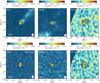 |
Fig. 1 ALMA Band 6 moment-zero images of the COM-rich sources analyzed in this study: B1-c (left), S68N (middle), and B1-bS (right). In color the spatial distribution of CH3 OH 21,1 –10,1 (top row, Eup = 28 K) and CH3 OCHO 217,14 –207,13 emission (bottom row, Eup = 170 K) is shown, with the color scale shown on top of each image. The images are integrated over [− 10,10] km s−1 with respect to the Vlsr. In the color bar, the 3σline level is indicated with the black bar, with σline = 4.0, 4.9, and 4.4 mJy beam−1 km s−1 for B1-c, S68N, and B1-bS, respectively. The continuum is shown with the black contours with increasing [3,5,8,12,18,21,30] σcont, where σcont is 1.5, 0.8, and 1.0 mJy beam−1 km s−1 for B1-c, S68N,and B1-bS, respectively. The size of the beam is shown in the lower right of each image, and in the lower left a scale bar is displayed. The image of B1-bS has a lower S/N since the source is located on the edge of the primary beam. |
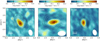 |
Fig. 2 Same as Fig. 1, but now for CH3OCH3 70,7 –61,6 (Eup = 25 K) in Band 3. Here, σline = 6.3, 5.5, and 5.2 mJy beam−1 km s−1 for B1-c, S68N, and B1-bS, respectively. The continuum contours are [3,5,8,12,18,21,30] σcont, where σcont is 0.46, 0.54, and 0.71 mJy beam−1 km s−1 for B1-c, S68N, and B1-bS, respectively. |
3.2 Column densities and excitation temperatures
The column densities and excitation temperatures of all COM-rich sources are presented in Appendix B. We considera derived column density an upper limit if the error is more than 80% of the corresponding best fitting value. The number of lines used for fitting each species is listed in Table B.2. Upper limits (3σ) to the column density are provided if no unblended lines are detected. For B1-c in Band 6, unambiguous detections (i.e., > 5 unblended lines identified) are made for 13CH3OH, CH OH, CH2DOH, CH3CHO, CH3OCHO, CH3OCH3, CH3COCH3, and aGg’(CH2OH)2. For S68N and B1-bS, line blending and sensitivity hampered unambiguous detections for several of these COMs, but tentative detections can still be made for most species. H2CCO and t-HCOOH show less than three detected transitions, and their identifications are therefore considered tentative. gGg’(CH2OH)2 and CH2OHCHO are only detected toward B1-c in Band 6; for all other sources (and B1-c Band 3) we put upper limits on the column density for an excitation temperature of 200 K. Due to the absence of any optically thin CH3OH lines in our data, the column density of CH3OH is determined by scaling it from 13CH3OH for Band 3 and CH
 OH for Band 6 (using 12C/13C ~ 70 and 16O/18O ~ 560 for the local ISM; Milam et al. 2005; Wilson & Rood 1994). In Fig. 3, part of the Band 6 spectrum of B1-c is shown with the best fitting model overlayed. The full Band 6 spectra with best-fit model of all sources can be found in Appendix C. The full Band 3 spectrum of B1-c is presented in Appendix D.
B1-c is the most COM-rich source of our sample. The measured column densities in Band 6 vary between 1.9 × 1018 cm−2 for CH3OH and 7.0 × 1014 cm−2 for t-HCOOH in a ~150 AU diameter region. Our derived column density for CH2OHCHO is 2.0 × 1015 cm−2. Most COMs show column densities on the order of ~ 1015−16 cm−2 in both Band 3 and Band 6.
The column densities toward S68N are a factor ~1.5−2 lower than toward B1-c. Similarly, the highest column density is derived for CH3OH (1.4 × 1018 cm−2), the lowest for t-HCOOH (9.1 × 1014 cm−2) in Band 6, and ~ 1015−16 cm−2 for most COMs.
B1-bS has the lowest column densities measured in this sample, up to an order of magnitude lower than toward B1-c with values of the order of ~ 1014−17 cm−2. This source was located at the edge of our ALMA field of view, resulting in a lower sensitivity and an increased level of noise. Our derived column densities (for a source size of 0.45″) are up to a factor of a few lower than those derived by Marcelino et al. (2018) for a 0.35″ source size, which is roughly the difference in beam dilution.
For molecules with multiple lines for which a Tex is derived, the average excitation temperature in Band 3 is ~ 30 K lower than in Band 6. The average FWHM for B1-c and S68N in Band 6 is 3.3 ± 0.2 and 5.0 ± 0.2 km s−1, respectively(the FWHM for B1-bS was fixed to 1 km s−1). In Band 3 this is 3.1 ± 0.2 and 4.5 ± 0.5, respectively.The average FWHM in Band 3 is therefore slightly lower than in Band 6 for B1-c and S68N, but within the uncertainties. This matches the expectation that the Band 3 observations trace the colder more extended regions and that Band 6 is more sensitive to warmer compact regions because the transition upper energies in Band 3 are on average lower than in Band 6 (see Tables E.2 and E.3) and because the beam size and LAS are larger. For all species for which Tex was fixed inBand 3, no significant changes in the column densities or abundances arise from decreasing excitation temperature by 30 K. In Table B.3, the results of a fit with Tex = 100 K to the Band 3 data are presented. The derived column densities are typically about a factor two lower than derived with Tex as a free parameter or fixed to 200 K.
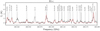 |
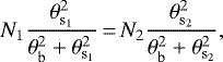
Fig. 3 Part of the Band 6 spectrum of B1-c shown in black with the best-fitting model overplotted in red. The window is centered around a few CH3CHO, CH3 OCHO, and CH3CH2OH lines. The focus here is on the O-bearing COMs; for this reason several transitions clearly visible in the data (i.e., CH3 CH2CN) do not showup in the fitting model. Lines in italics were excluded during the fitting. |
Column densities of CH3OH and abundance fractions (%) with respect to CH3OH for all COM rich sources.
3.3 Relative abundances
Clear isotopolog detections are only made for methanol. The 13CH3OH/CH OH abundance ratio is less than 6 for all targets, which is lower than the elemental value of approximately 8. This hints at the possibility that even 13CH3OH is optically thick for these sources. The CH2DOH/CH3OH ratio is on the order of ~1−10%. Hints for features of isotopologs are seen for partially deuterated ethanol (CH2DCH2OH) and methyl formate (CH3O13CHO), but these lines are too weak to allow unambiguous confirmation or to derive physical properties.
In order to compare our derived column densities, we determine the abundance ratios of each species with respect to CH3OH. Because CO, which is the usual tracer of H2, comes from more extended regions, CH3OH is chosen as the reference species. In Table 2, the derived abundances are presented for the three COM-rich sources. The abundances vary between B1-c and S68N within a factor of two to three. This may simply be an effect of the source properties; the lines in S68N are, for example, a factor ~ 1.5 broader (~ 5.0 and ~ 3.3 km s−1 in Band 6, respectively) resulting in more blended lines. In S68N, our abundances of CH3OCHO, CH3OCH3, and H2CCO are an order of magnitude lower than those derived by Bergner et al. (2019). The discrepancies are potentially due to different approaches to optical depth correction. Our observations of B1-bS have a low S/N. Nevertheless our derived abundance ratios coincide within a factor of a few with the hot (200 K) component modeled by Marcelino et al. (2018).
The abundances in Band 3 for B1-c deviate within a factor of approximately two from the abundances derived in Band 6. Only CH3CHO and t-HCOOH are more abundant based on the Band 3 data. In S68N, CH3OCHO is less abundant in Band 3 whereas CH3OCH3 is more abundant. In B1-bS, both CH3OCHO and CH3OCH3 are significantly more abundant in Band 3, possibly because the column density of CH3OH is underestimated.
4 Discussion
4.1 Occurrence of COMs in young protostars
The emission of COMs is assumed to originate from inside the Tdust ~ 100−300 K radius. Using the relation of Bisschop et al. (2007) for the 100 K radius in hot cores:
 (2)
(2)
with L the source luminosity, implies an RT = 100 K of 37.4, 35.8, and 11.6 AU for B1-c, S68N, and B1-bS, respectively. Our Band 6 beam size of ~ 0.45″ (corresponding to a radius of ~72 and ~98 AU for Perseus and Serpens, respectively) is larger than this radius and thus agrees with all COM emission being unresolved, except for any CH3OH emission related to an outflow.
Previous studies have found that a higher luminosity implies more emission of COMs (e.g., Jørgensen et al. 2002; Young & Evans 2005; Visser et al. 2009). Following Eq. (2) we would indeed expect the occurrence of COM emission to be correlated to the source luminosity. Here, three of the seven sources studied show emission of COMs. However, our most luminous source, SMM3, does not exhibit any COM emission. On the other end, the two sources with the lowest luminosity, B1-bN and B1-b, do not show any COM emission either. Interestingly, B1-bS also has a rather low luminosity but does exhibit COM emission. This suggests that, for the targets that we observed, no clear correlation exists between the occurrence of gaseous COMs and source luminosity.
Not finding such a correlation is surprising. However, the relation for RT = 100 K in Eq. (2) assumes a spherically symmetric infalling envelope (Bisschop et al. 2007). In reality, our Class 0 sources may be surrounded by an accretion disk (e.g., Tobin et al. 2012; Murillo et al. 2013). The presence of a disk or disk-like structure may shift the RT = 100 K inwards as the temperature in the midplane of a disk-like structure is lower than in the surface layers (e.g., Jørgensen et al. 2005; Visser et al. 2009). However, even for a fixed RT = 100 K, the amount of material with Tdust > 100 K (e.g., high enough to release the COMs from the dust grains) can vary between different sources due to, for example, differences in the disk mass and radius (Persson et al. 2016).
The absence of COM emission can also originate from other source properties. B1-bN has been suggested as a first hydrostatic core candidate (e.g., Pezzuto et al. 2012; Hirano & Liu 2014; Gerin et al. 2017); the temperature in the inner regions may not have reached the threshold for ice COM sublimation. B1-b has a high bolometric temperature, and could therefore be more evolved than the other sources. Here, only a weak continuum is detected, indicating that B1-b may have a cleared inner region; all gaseous COMs have either already been destroyed or are incorporated as ices in the cold outer part. The strong ice absorption observed toward this source might originate in a region that is more extended than the inner B1-b envelope (Öberg et al. 2011). SMM3 shows strong continuum, which may imply that increased dust opacity hides any COM emission.
Despite the absence of a clear correlation between the occurrence of COM emission and source luminosity, an increase in luminosity should result in higher temperatures and an increased UV radiation field (Visser et al. 2009; Drozdovskaya et al. 2016). The abundance of COMs with respect to CH3OH may therefore be related to the source luminosity. However, Taquet et al. (2015) and Belloche et al. (2020) have shown that for most COM abundances, no clear correlation exists with luminosity, similar to what is found here; see Fig. 4. Our range of source luminosities is significantly smaller (up to ~ 20 L⊙ compared to 106 L⊙; Taquet et al. 2015), and a similar scatter of abundances can be seen for their lower luminosities.
 |
Fig. 4 Abundance of CH2DOH (top left), CH3CH2OH (top right), CH3OCHO (bottom left), and CH3OCH3 (bottom right) with respect to CH3OH as a function of bolometric source luminosity. Both the abundances in Band 3 (blue) and Band 6 (red) are plotted; the Band 3 data points are slightly shifted in luminosity for clarity. Arrows denote upper limits. In gray, the abundances of IRAS 2A and IRAS 4A (Taquet et al. 2015, 2019), HH 212 (Lee et al. 2019a), IRAS 16293A (Manigand et al. 2020), and IRAS 16293B (Jørgensen et al. 2018) are presented. |
4.2 Dependence on source size
In modeling the COM emission, a source size equal to the beam size (0.45″) was assumed for all sources. However, since the emission is spatially unresolved, the source size in reality will be smaller. A smaller emitting region will increase the derived column densities, and may result in spectral lines actually being optically thick. We can test this scenario by assuming the 100 K diameter as a source size. This gives an emitting region of 0.23″, 0.16″, and 0.07″ for B1-c, S68N, and B1-bS, respectively. Assuming the lines remain optically thin, the column densities derived for a 0.45″ source size can be scaled to a smaller size by computing the difference in beam dilution (see Eq. (1)):
 (3)
(3)
where N1,2 are the column densities for respective source sizes  , and θb is the beam size.
For B1-c and S68N, the resulting column densities still give optically thin (τ < 0.1) lines for all species except CH3OH. However, the lines of CH3OH are already optically thick for a 0.45″ source size and the column density is derived from the 13C and 18O isotopologs, whose lines remain optically thin. This means that the abundances derived above in Table 2 for these two sources remain the same. However, for B1-bS, most lines become optically thick (i.e., τ > 0.1), indicating that the abundances derived in Table 2 for B1-bS should be used with care.
4.3 Fromcold (Band 3) to hot (Band 6) COMs
The temperature in the envelopes of Class 0 sources is expected to have an “onion” layered shell structure, with increasing temperature when moving closer to the star (e.g., Jørgensen et al. 2002). In warmer layers, the COMs could be further processed to form more complex molecules (on the dust grains) and, more importantly, will all be released from the dust grains when the temperature reaches Tdust ≈ 100−300 K. With our multi-band observations, we can check for hints of this onion-layered temperature structure by comparing the excitation temperature of COMs in Band 3, which is more sensitive to extended emission, to the COMs in Band 6, which is more sensitive to compact emission. Indeed, the average excitation temperature for the few species for which an excitation temperature could be derived in Band 3 (i.e., CH3CH2OH, CH3OCHO, and CH3OCH3) is about 30 K lower than in Band 6. However, as mentioned in Sect. 3.2, no significant changes in the column densities and abundances arise if the Band 3 excitation temperature of all species for which Tex was fixed is decreased by 30 K. The outcome of the Band 6 model does not change when all lines with a low Eup < 100 K are excluded.
Jørgensen et al. (2018) modeled the abundances of O-bearing COMs in IRAS 16293B and found that they can be divided in two classes with temperatures of ~ 125 K (warm) and ~ 300 K (hot). Most COMs in our sample have excitation temperatures of ~ 200 K, which falls in the middle between these two classes. Only CH3OCH3 consistently shows Tex ~ 100 K, both in the Band 3 and Band 6 observations for all sources. This agrees with Jørgensen et al. (2018), who classified CH3OCH3 as a warm species. However, some ambiguity remains, since CH3OCH3 is also observed to have hot components in, for instance, higher mass cores (Belloche et al. 2013; Isokoski et al. 2013).
The emission of COMs can be a superposition of a warm/hot inner component, and a second colder and more extended component. Earlier observational studies have shown that indeed a cold (T < 100 K, i.e., below the desorption temperature), more extended component may be present (e.g., Bisschop et al. 2007; Isokoski et al. 2013; Fayolle et al. 2015; Marcelino et al. 2018). Using our data, a possible cold component can be probed by fitting a multi-component model to the Band 3 data. This is only done for B1-c and S68N since the S/N of B1-bS in Band 3 is insufficient to carry out such an analysis. H2 CCO, CH3COCH3, (CH2OH)2, and CH2OHCHO are excluded from this analysis due to the lack of clear detections in our Band 3 data.
For the warm/hot component, the best-fit model of Band 6 is adopted. This component is kept fixed. As a second component, a colder model is introduced. Here, an excitation temperature of 60 K was assumed and only the column density was fitted for. The FWHM was initially set as a free parameter, but fixed to that of the warm/hot component in the cases where fit results were unconstrained. A source size of 2.0″ (equal to Band 3 beam) is assumed for the cold component, compared with the source size of the warm component of 0.45″.
The results are presented in Table 3. Figure 5 shows part of the Band 3 spectrum of B1-c centered around several CH3OCHO lines. The abundances of Table 3 are presented in a bar plot in Fig. 6. In B1-c, a cold (Tex = 60 K) and more extended component is detected for most species. The column density of this cold component is typically a few percent but can rise up to 10% of the warm/hot inner component. The abundances of more complex species in the cold component are higher than those in the warm/hot component, which contradicts the idea that COMs are more effectively processed and released from icy grains in warmer layers. However, we highlight the fact that the column density of 13CH3OH, and therefore CH3OH, is likely underestimated.
Only for CH3CH2OH and CH3OCHO could a FWHM of 3.3 ± 0.8 be derived for the cold component which agrees with the average FWHM of the warm/hot component of 3.3 ± 0.2. The line width of the cold component can be expected to be smaller since the emitting material is located further out in the envelope. However, Murillo et al. (2018) find that lower resolution data can also result in a larger line width, especially if the molecule is associated with the outflow or its cavity.
The presence of a cold component of COM emission indicates that some gas-phase formation routes are already efficient in the cold envelope as most COMs formed through grain-surface chemistry are still frozen out at these temperatures. Alternatively, this could indicate that other mechanisms are capable of transferring the COMs from the solid state to the gas phase. Possible mechanisms include photodesorption (Fayolle et al. 2011; Muñoz Caro et al. 2016), desorption of fragments following photo-dissociation (Bertin et al. 2016), low-temperature co-desorption (Fayolle et al. 2013; Ligterink et al. 2018c), or reactive desorption via a thermal hot-spot (Minissale et al. 2016; Chuang et al. 2018). Only for CH3OCH3 and the deuterated and 18O isotopologs of CH3OH does an extended component seem to be absent.
Formic acid is very abundant in the cold, extended component. This disagrees with the hot identification in IRAS 16293B (Jørgensen et al. 2018), but is more consistent with the cold identification in high-mass star-forming regions (Bisschop et al. 2007; Belloche et al. 2013) and that HCOOH is likely an abundant ice species (Öberg et al. 2011; Boogert et al. 2015). However, in both Band 3 and Band 6, only one to three lines could be fitted, and therefore the identification of t-HCOOH should be considered rather tentative.
In S68N, a cold component is less evident. Only for CH3OCHO is a cold column density derived; for all other species only upper limits are found. These results suggest that a possible cold component would have a column density of ≲1% of the warmcomponent.
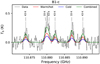 |
Fig. 5 Part of the Band 3 spectrum of the warm/hot (Tex ~ 100−300 K) compact (red), cold (Tex = 60 K) extended (blue), and combined (green) model overlayed on the data (black). The spectral features are from CH3 OCHO, with the upper energy indicated on top. |
Column densities resulting from the multi-component analysis.
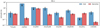 |
Fig. 6 Abundance of several species with respect to CH3OH for our multi-component analysis. The warm (Tex ~ 200 K) component is fixed to the Band 6 model with a 0.45″ source size, whereas the cold (Tex = 60 K) component is fitted with a more extended 2.0″ source size. The 2σ (95%) errors are shown in black, with arrows denoting upper limits. The CH3 OH column density is determined by scaling from 13CH3OH using 12C∕13C = 70 and 16O∕18O = 560, respectively.The higher abundances in the cold component are likely due to an underestimate of the column density of 13CH3OH. |
4.4 Comparison to other sources
Our Band 6 abundances are compared to the ALMA Band 7 abundances of IRAS 16293B (Jørgensen et al. 2018)and HH 212 (Lee et al. 2019a); see Fig. 7. The abundances of several COMs (i.e., CH2DOH, CH3OCHO, CH3OCH3, and CH3COCH3) from this work are very similar to IRAS 16293B and HH 212; the distribution of abundances seems to span only a factor of a few. The abundances are also within a factor three of IRAS 2A and IRAS 4A (Taquet et al. 2015). This similarity in abundances is rather interesting given that the source properties (e.g., Lbol, Tbol, etc.) are different for all sources. For example, IRAS 2A has a luminosity of 36 L⊙, whereas the luminosity of B1-bS is two orders of magnitude lower (0.57 L⊙). A similarly large range is seen for the bolometric temperature and envelope mass. Moreover, these sources originate from four different star-forming regions: Perseus (B1-bS, B1-c, IRAS 2A, IRAS 4A), Serpens (S68N), Ophiuchus (IRAS 16293B), and Orion (HH 212). It appears that, despite the differences in source properties and local environment, the internal distribution of these COM abundances is roughly similar. This indicates that their formation schemes must follow a similar recipe, for instance following the atom addition and abstraction reaction networks proposed to govern the surface chemistry in cold interstellar clouds (e.g., Chuang et al. 2016). This implies that solid-state processes are already enriching the complex organic inventory of the interstellar medium in the prestellar phase.
Interestingly, our sources are under-abundant up to more than one order of magnitude in CH3CH2OH, CH3CHO, and CH2OHCHO compared with IRAS 16293B, HH 212, IRAS 2A, and IRAS 4A. Our abundances of these COMs fall within a factor of a few with IRAS 16293A (Manigand et al. 2020). This suggests that for some COMs, local source conditions do become important for the formation or the destruction. The column density ratio of CH3OCHO to CH2OHCHO of B1-c is consistent with the lower part of the bimodal distribution found by El-Abd et al. (2019). For H2CCO and t-HCOOH, our sources also have lower abundances. The abundance of t-HCOOH in the cold component of the multi-component analysis (see Sect. 4.3) is consistent with IRAS 16293B and HH 212. However, the detections of these species are rather tentative since only less than three clear unblended lines (not taking into account (hyper)fine structured lines) are detected.
In more massive star-forming regions, a larger scatter in COM abundances seems to be present. AFGL 4176 has abundances very similar to ours for most COMs (Bøgelund et al. 2019), whereas those in Orion KL show deviations: the abundance of CH3CH2OH is similar (Tercero et al. 2018), but CH3OCHO, CH3OCH3 have lower abundances in our sources, and CH3COCH3 higher abundances (see Table 6 in Bøgelund et al. 2019). Even larger deviations are found toward Sagittarius B2, where the abundances of all COMs are higher by up to an order of magnitude (Belloche et al. 2016).
The abundances derived here are higher than those in chemical models of a collapsing cloud for most COMs (e.g., Garrod 2013). Especially for CH3COCH3 and (CH2OH)2, these models underestimate the abundances by up to an order of magnitude. This may be a direct result of a still not fully characterized solid-state and gas-phase chemistry and underlying gas–grain interactions (see discussion by Bøgelund et al. 2019).
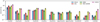 |
Fig. 7 Bar plot comparing our derived Band 6 abundances to those of other sources. The IRAS 16293B abundances for all species except (CH2OH)2, CH2 OHCHO, and CH3COCH3 are from Jørgensen et al. (2018); the (CH2OH)2 and CH2OHCHO abundances are from Jørgensen et al. (2016), and the CH3COCH3 abundances from Lykke et al. (2017). The HH 212 abundances are from Lee et al. (2019a). The 2σ (95%) errors are shown in black, with arrows denoting upper limits. We note that the abundances of our targets are remarkably similar and show comparable values to those derived for IRAS 16293B and HH 212. |
4.5 Comparison with ices
No clear COM ice features have yet been observed toward any of our COM-rich sources. However, hints for CH3CHO, CH3CH2OH, and t-HCOOH ice have been detected toward B1-b (from the same cloud as B1-c) with an abundance of ~ 10% with respect to CH3OH (Öberg et al. 2011; Boogert et al. 2015). These are higher than those derived for the gaseous warm/hot component in this work (~ 0.1−1%). A possible explanation for this is that, besides typical grain-surface chemistry, additional gas-phase chemistry following thermal desorption in the warm inner envelope can contribute to further processing the COMs into more complex species.
To better compare the abundances of COMs in the ice and gas phase, it is essential to directly observe the ices. However, the above mentioned detections are still very uncertain, with only CH3OH being securely identified in interstellar ices. Measuring the column densities of interstellar COM ices remains difficult because current infrared telescopes lack the sensitivity or wavelength coverage, and because the spectral features originating from ices are broad and depend on the ice composition. Moreover, the number of COMs for which extensive high-resolution infrared laboratory spectra have become available is limited (Hudson et al. 2018; Terwisscha van Scheltinga et al. 2018). Future mid-infrared facilities such as JWST/MIRI will allow COMs to be directly observed in the ice, which will be essential for studying their formation and evolution from the cold envelope toward the warm inner regions.
4.6 Temperature dependence of deuterated methanol
The deuteration fraction of methanol is an indication of the temperature during the solid-state formation of this species. At low temperatures, deuterium is more efficient than regular hydrogen in the hydrogenation process on interstellar dust grains (e.g., Nagaoka et al. 2005). This leads to a higher deuteration fraction than the elemental ratio (D ∕H ~ 10−5; Caselli & Ceccarelli 2012). Bøgelund et al. (2018) investigated the effect of temperature during the formation of methanol with the astrochemical GRAINOBLE model (Taquet et al. 2012). In order to compare our methanol D/H ratios to their model results, our gas-phase CH2DOH abundances have to be corrected for statistical weights; a D atom has a three-times-higher probability of sticking into the CH3 group than into the OH group. In Band 3, this gives a D/H ratio of 1.9 ± 0.7, < 4.3, and < 3.3% for B1-c, S68N, and B1-bS respectively. In Band 6, this is 2.7 ± 0.9, 1.4 ± 0.6, and < 1.6%. These deuteration fractions correspond to a temperature during the formation of methanol of ~ 15 K, where a density of nH = 105−6 cm−3 was assumed (cf. Fig. 8 of Bøgelund et al. 2018).
Our derived methanol D/H fractions agree well with other well-studied low-mass protostars such as IRAS 16293B (~ 2%; Jørgensen et al. 2018), IRAS 2A and IRAS 4A (~2 and ~1%, respectively; Taquet et al. 2019), and HH 212 (~1% after taking into account statistical weights; Bianchi et al. 2017; Taquet et al. 2019). Our fractions are up to an order of magnitude higher than for high-mass star-forming regions such as NGC 6334I (~ 0.1% on average; Bøgelund et al. 2018), and Sagittarius B2 (0.04% after statistical correction; Belloche et al. 2016). The lower D/H ratios in more massive star-forming regions hint at a higher temperature (i.e., >20 K) already during the earliest phase of high-mass star formation.
5 Summary
In this paper, the content of oxygen bearing COMs is studied in seven young protostellar systems. High-resolution ALMA observationsin both Band 3 and Band 6 were used to determine the column densities and excitation temperatures. The main conclusions are as follows:
-
Three out of the seven sources exhibit warm COM emission features with typical Tex ~ 200 K. There seems to be no correlation between the bolometric luminosity (and temperature) and occurrence of COMs of these Class 0 sources. Other effects, such as disk formation and clearing of an inner region, may play a role as well.
-
A multi-component model was introduced to check whether a cold (Tex = 60 K), more extended component of COM emission is present. Only B1-c shows clear signs of such a cold component, with typicallya few percent of the column density of the warm component. This indicates that in the cold envelope already gas-phase formation may take place and that this could be a direct consequence of the grain-gas transitions of COMs or (radical) COM fragments. t-HCOOH is significantly more abundant in the cold component, hinting at the cold origin of this species.
-
The abundance of several COMs (i.e., CH2DOH, CH3OCHO, CH3OCH3, CH3COCH3, and (CH2OH)2) are remarkably similar in comparison to other young Class 0 protostars in different star-forming regions such as IRAS 16293-2422B and HH 212. This similarity suggests that the distribution of these COM abundances is roughly fixed at an early, cold, i.e., prestellar, stage. However, the abundances of some COMs (i.e., CH3CH2OH, CH3CHO, and CH2OHCHO) in our sources differ significantly from those found for IRAS 16293B and HH 212, possibly because local source conditions become important and affect formation and destruction pathways in different ways. Astrochemical modeling will be needed to further investigate these findings.
-
The D/H ratio of deuterated CH3OH is around a few percent for all COM-rich sources, suggesting a dust temperature of ~15 K during its solid-state formation. The derived formation temperature is similar to that found for other low-mass protostars, but is lower than that found in high-mass star-forming regions (>20 K).
Our sample of COM-rich protostars studied on Solar System scales remains small. How much of the prestellar cloud material is reprocessed during evolution toward protostellar systems and more evolved sources remains unknown. The abundance of most COMs in the ice phase is still highly uncertain. Future mid-infrared facilities, most notably the JWST, will provide vital information on COM ices. A larger sample of COM-rich sources with ALMA, both in the Class 0 phase and in the more evolved Class I phase where most COM emission has already disappeared, would provide better constraints on the chemical complexity during these earliest phases of star formation. The present work already shows that such studies will be valuable, given the rich distribution in COMs discussed here.
Acknowledgements
We would like to thank the anonymous referee for his/ her constructive comments on the manuscript. This paper makes use of the following ALMA data: ADS/JAO.ALMA#2017.1.01174.S and ADS/JAO. ALMA#2017.1.01350.S. ALMA is a partnership of ESO (representing its member states), NSF (USA) and NINS (Japan), together with NRC (Canada), MOST and ASIAA (Taiwan), and KASI (Republic of Korea), in cooperation with the Republic of Chile. The Joint ALMA Observatory is operated by ESO, AUI/NRAO and NAOJ. Astrochemistry in Leiden is supported by the Netherlands Research School for Astronomy (NOVA). B.T. acknowledges support from the Dutch Astrochemistry Network II with project number 614.001.751, financed by the Netherlands Organisation for Scientific Research (NWO). H.B. acknowledges support from the European Research Council under the Horizon 2020 Framework Program via the ERC Consolidator Grant CSF-648505. H.B. also acknowledges support from the Deutsche Forschungsgemeinschaft (DFG) via Sonderforschungsbereich (SFB) 881 “The Milky Way System” (sub-projectB1).
Appendix A Laboratory spectroscopic data
All laboratory spectroscopic data were acquired using the CDMS (Müller et al. 2001, 2005; Endres et al. 2016) and JPL (Pickett et al. 1998)catalogs. In some of the entries, vibrational or torsional states are not taken into account in the calculation of the partition function. At low temperatures, the contribution of these states are negligible. However, at higher temperatures (i.e., T >100 K), a so-called vibrational correction factor must be applied if the torsional and vibrational states are not accounted for in the partition functions. Below, we detail the laboratory spectroscopy of each individual species discussed in this paper and indicate if a vibrational correction factor was applied.
The data of CH3OH are taken from the CDMS database and are based on the work of Xu et al. (2008). The ground state and first three torsional states are taken into account in the partition function. The entry of the 13C isotopolog takes the first two torsional states into account (Xu & Lovas 1997). These latter authors assumed that the dipole moment is the same as the main isotopolog and calculated the partition function taking only the permanent dipole moment into account. The CH OH entry is based mostly on the data of Fisher et al. (2007). The spectroscopic data of CH2DOH are taken from the JPL catalog, where the entry is based on the work of Pearson et al. (2012). The vibrational correction factor at 200 K is calculated to be 1.181 by summing up over torsional substates extrapolated from Lauvergnat et al. (2009).
CH3CH2OH exists as two conformers: trans and gauche, which originates from the torsion in the OH group. The spectroscopic data are taken from the CDMS catalog, where the entry is based on Pearson et al. (2008) and updated by Müller et al. (2016), who noticed that the old catalog entry did not predict the line intensities correctly around 3 mm in Sagittarius B2. This applies also to other frequency regions, but not to all transitions. Both conformers are included in the entry.
The data of CH3CHO are taken from the JPL catalog. It is based on laboratory spectroscopy of Kleiner et al. (1996) and includes the first and second torsional state in its partition function.
The spectroscopic data of CH3OCHO are taken from the JPL database. The entry is based on the work of Ilyushin et al. (2009) and Brown et al. (1975). The partition function includes states up to the first torsional state.
CH3OCH3 data are taken from the CDMS entry, which includes mostly the work of Endres et al. (2009). The partition function includes the ground vibrational state and excited states up to 500 cm−1. However, for the excitation temperatures derived in this work (~100 K), the contribution of higher order vibrational states to the partition function is negligible.
The CH3COCH3 data are taken form the JPL catalog. The rotational transitions were calculated by Groner et al. (2002) and include only the ground state. Here, we use an updated version of the entry. It is based on the study of Ordu et al. (2019) with the majority of the lines from Groner et al. (2002).
The (CH2OH)2 structure consists of three coupled rotors, which give rise to ten different stable configurations (Christen et al. 2001). Here, only the two lowest energy conformers of (CH2OH)2 are studied. The aGg’ state is the lowest energy state whereas the gGg’ state lies about 290 K above that (Müller & Christen 2004). The spectroscopic data are taken from the CDMS entries, which are based on the work of Christen et al. (1995) and Christen & Müller (2003) for the aGg’ conformer and Christen et al. (2001) and Müller & Christen (2004) for the gGg’ conformer. For gGg’(CH2OH)2, the partition function and line intensities were calculated assuming as if it is the lowest energy state conformer. For these calculations, only the ground state is considered, and therefore we approximate the effect of vibrational states using a vibrational correction factor of 2.143 for both conformers at 200 K.
The CH2OHCHO data are taken from the CDMS catalog. The entry is based on the work of Butler et al. (2001) and only includes data on the ground vibrational state. A vibrational correction factor of 1.5901 is calculated at 200 K in the harmonic approximation.
The spectroscopic data of H2CCO are acquiredfrom the CDMS catalog. The entry is calculated mostly by Johnson & Strandberg (1952), Fabricant et al. (1977), and Brown et al. (1990). The contribution of vibrational states is assumed to be negligible.
Formic acid, HCOOH, exists both in a trans and cis state, where the lowest energy state of c-HCOOH is about 2000 K higher than for t-HCOOH. In this study we only detect t-HCOOH, for which we use the entry of the JPL catalog. This is based on the work of Bellet et al. (1971). The vibrational correction is < 1.1 at 200 K and is therefore neglected.
Appendix B CASSIS modeling results
Computed Band 3 and Band 6 column densities and excitation temperatures of our sources.
Number of transitions and lines fitted for all sources.
Computed column densities and abundance ratios in Band 3, assuming Tex = 100 K.
Appendix C Full ALMA Band 6 spectra
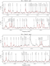 |
Fig. C.1 FullBand 6 spectrum of B1-c (black) with best fitting CASSIS model overplotted (red). We indicate the positions of species, where lines in italic are excluded in the fitting. Lines annotated with an “X” are unidentified. |
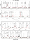 |
Fig. C.1 continued. |
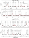 |
Fig. C.2 continued. |
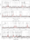 |
Fig. C.3 continued. |
Appendix D B1-c Band 3 spectrum
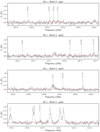 |
Fig. D.1 Full Band 3 spectrum of B1-c (black) with best fitting CASSIS model overplotted (red). We indicate the positions of species, where lines in italic are excluded in the fitting. |
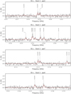 |
Fig. D.1 continued. |
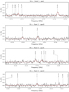 |
Fig. D.1 continued. |
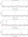 |
Fig. D.1 continued. |
References
- Arce, H. G., Santiago-García, J., Jørgensen, J. K., Tafalla, M., & Bachiller, R. 2008, ApJ, 681, L21 [NASA ADS] [CrossRef] [Google Scholar]
- Artur de la Villarmois, E., Jørgensen, J. K., Kristensen, L. E., et al. 2019, A&A, 626, A71 [NASA ADS] [CrossRef] [EDP Sciences] [Google Scholar]
- Balucani, N., Ceccarelli, C., & Taquet, V. 2015, MNRAS, 449, L16 [Google Scholar]
- Bellet, J., Samson, C., Steenbeckliers, G., & Wertheimer, R. 1971, J. Mol. Struct., 9, 49 [NASA ADS] [CrossRef] [Google Scholar]
- Belloche, A., Müller, H. S. P., Menten, K. M., Schilke, P., & Comito, C. 2013, A&A, 559, A47 [NASA ADS] [CrossRef] [EDP Sciences] [Google Scholar]
- Belloche, A., Müller, H. S. P., Garrod, R. T., & Menten, K. M. 2016, A&A, 587, A91 [NASA ADS] [CrossRef] [EDP Sciences] [Google Scholar]
- Belloche, A., Maury, A. J., Maret, S., et al. 2020, A&A, 635, A198 [CrossRef] [EDP Sciences] [Google Scholar]
- Bergner, J. B., Öberg, K. I., Garrod, R. T., & Graninger, D. M. 2017, ApJ, 841, 120 [NASA ADS] [CrossRef] [Google Scholar]
- Bergner, J. B., Martín-Doménech, R., Öberg, K. I., et al. 2019, ACS Earth Space Chem., 3, 1564 [CrossRef] [Google Scholar]
- Bertin, M., Romanzin, C., Doronin, M., et al. 2016, ApJ, 817, L12 [NASA ADS] [CrossRef] [Google Scholar]
- Bianchi, E., Codella, C., Ceccarelli, C., et al. 2017, A&A, 606, L7 [NASA ADS] [CrossRef] [EDP Sciences] [Google Scholar]
- Bisschop, S. E., Jørgensen, J. K., van Dishoeck, E. F., & de Wachter, E. B. M. 2007, A&A, 465, 913 [NASA ADS] [CrossRef] [EDP Sciences] [Google Scholar]
- Bøgelund, E. G., McGuire, B. A., Ligterink, N. F. W., et al. 2018, A&A, 615, A88 [NASA ADS] [CrossRef] [EDP Sciences] [Google Scholar]
- Bøgelund, E. G., Barr, A. G., Taquet, V., et al. 2019, A&A, 628, A2 [NASA ADS] [CrossRef] [EDP Sciences] [Google Scholar]
- Boogert, A. C. A., Pontoppidan, K. M., Knez, C., et al. 2008, ApJ, 678, 985 [NASA ADS] [CrossRef] [Google Scholar]
- Boogert, A. C. A., Gerakines, P. A., & Whittet, D. C. B. 2015, ARA&A, 53, 541 [Google Scholar]
- Bottinelli, S., Ceccarelli, C., Lefloch, B., et al. 2004, ApJ, 615, 354 [NASA ADS] [CrossRef] [Google Scholar]
- Brown, R. D., Crofts, J. G., Gardner, F. F., et al. 1975, ApJ, 197, L29 [NASA ADS] [CrossRef] [Google Scholar]
- Brown, R. D., Godfrey, P. D., McNaughton, D., Pierlot, A. P., & Taylor, W. H. 1990, J. Mol. Struct., 140, 340 [Google Scholar]
- Butler, R. A. H., De Lucia, F. C., Petkie, D. T., et al. 2001, ApJS, 134, 319 [NASA ADS] [CrossRef] [Google Scholar]
- Calcutt, H., Jørgensen, J. K., Müller, H. S. P., et al. 2018, A&A, 616, A90 [NASA ADS] [CrossRef] [EDP Sciences] [Google Scholar]
- Caselli, P., & Ceccarelli, C. 2012, A&ARv, 20, 56 [NASA ADS] [CrossRef] [MathSciNet] [Google Scholar]
- Charnley, S. B., Tielens, A. G. G. M., & Millar, T. J. 1992, ApJ, 399, L71 [NASA ADS] [CrossRef] [Google Scholar]
- Christen, D., & Müller, H. S. P. 2003, Phys. Chem. Chem. Phys., 5, 3600 [CrossRef] [Google Scholar]
- Christen, D., Coudert, L. H., Suenram, R. D., & Lovas, F. J. 1995, J. Mol. Spectr., 172, 57 [NASA ADS] [CrossRef] [Google Scholar]
- Christen, D., Coudert, L. H., Larsson, J. A., & Cremer, D. 2001, J. Mol. Spectr., 205, 185 [NASA ADS] [CrossRef] [Google Scholar]
- Chuang, K. J., Fedoseev, G., Ioppolo, S., van Dishoeck, E. F., & Linnartz, H. 2016, MNRAS, 455, 1702 [Google Scholar]
- Chuang, K. J., Fedoseev, G., Qasim, D., et al. 2017, MNRAS, 467, 2552 [NASA ADS] [Google Scholar]
- Chuang, K. J., Fedoseev, G., Qasim, D., et al. 2018, ApJ, 853, 102 [NASA ADS] [CrossRef] [Google Scholar]
- Coutens, A., Ligterink, N. F. W., Loison, J. C., et al. 2019, A&A, 623, L13 [NASA ADS] [CrossRef] [EDP Sciences] [Google Scholar]
- Crockett, N. R., Bergin, E. A., Neill, J. L., et al. 2014, ApJ, 787, 112 [NASA ADS] [CrossRef] [Google Scholar]
- Drozdovskaya, M. N., Walsh, C., van Dishoeck, E. F., et al. 2016, MNRAS, 462, 977 [NASA ADS] [CrossRef] [Google Scholar]
- El-Abd, S. J., Brogan, C. L., Hunter, T. R., et al. 2019, ApJ, 883, 129 [CrossRef] [Google Scholar]
- Endres, C. P., Drouin, B. J., Pearson, J. C., et al. 2009, A&A, 504, 635 [NASA ADS] [CrossRef] [EDP Sciences] [Google Scholar]
- Endres, C. P., Schlemmer, S., Schilke, P., Stutzki, J., & Müller, H. S. P. 2016, J. Mol. Spectr., 327, 95 [NASA ADS] [CrossRef] [Google Scholar]
- Enoch, M. L., Evans, Neal J., I., Sargent, A. I., & Glenn, J. 2009, ApJ, 692, 973 [NASA ADS] [CrossRef] [Google Scholar]
- Enoch, M. L., Corder, S., Duchêne, G., et al. 2011, ApJS, 195, 21 [NASA ADS] [CrossRef] [Google Scholar]
- Fabricant, B., Krieger, D., & Muenter, J. S. 1977, J. Chem. Phys., 67, 1576 [NASA ADS] [CrossRef] [Google Scholar]
- Fayolle, E. C., Bertin, M., Romanzin, C., et al. 2011, ApJ, 739, L36 [NASA ADS] [CrossRef] [Google Scholar]
- Fayolle, E. C., Bertin, M., Romanzin, C., et al. 2013, A&A, 556, A122 [NASA ADS] [CrossRef] [EDP Sciences] [Google Scholar]
- Fayolle, E. C., Öberg, K. I., Garrod, R. T., van Dishoeck, E. F., & Bisschop, S. E. 2015, A&A, 576, A45 [NASA ADS] [CrossRef] [EDP Sciences] [Google Scholar]
- Fayolle, E. C., Öberg, K. I., Jørgensen, J. K., et al. 2017, Nat. Astron., 1, 703 [NASA ADS] [CrossRef] [Google Scholar]
- Fedoseev, G., Chuang, K. J., Ioppolo, S., et al. 2017, ApJ, 842, 52 [NASA ADS] [CrossRef] [Google Scholar]
- Fisher, J., Paciga, G., Xu, L.-H., et al. 2007, J. Mol. Spectr., 245, 7 [NASA ADS] [CrossRef] [Google Scholar]
- Fuchs, G. W., Cuppen, H. M., Ioppolo, S., et al. 2009, A&A, 505, 629 [NASA ADS] [CrossRef] [EDP Sciences] [Google Scholar]
- Garrod, R. T. 2013, ApJ, 765, 60 [Google Scholar]
- Garrod, R. T., & Herbst, E. 2006, A&A, 457, 927 [NASA ADS] [CrossRef] [EDP Sciences] [Google Scholar]
- Garrod, R. T., Widicus Weaver, S. L., & Herbst, E. 2008, ApJ, 682, 283 [NASA ADS] [CrossRef] [Google Scholar]
- Gerakines, P. A., Schutte, W. A., & Ehrenfreund, P. 1996, A&A, 312, 289 [NASA ADS] [Google Scholar]
- Gerin, M., Pety, J., Commerçon, B., et al. 2017, A&A, 606, A35 [NASA ADS] [CrossRef] [EDP Sciences] [Google Scholar]
- Groner, P., Albert, S., Herbst, E., et al. 2002, ApJS, 142, 145 [NASA ADS] [CrossRef] [Google Scholar]
- Harsono, D., Bjerkeli, P., van der Wiel, M. H. D., et al. 2018, Nat. Astron., 2, 646 [NASA ADS] [CrossRef] [Google Scholar]
- Hatchell, J., Fuller, G. A., & Richer, J. S. 2007, A&A, 472, 187 [NASA ADS] [CrossRef] [EDP Sciences] [Google Scholar]
- Herbst, E., & van Dishoeck, E. F. 2009, ARA&A, 47, 427 [NASA ADS] [CrossRef] [Google Scholar]
- Hirano, N., & Liu, F.-c. 2014, ApJ, 789, 50 [NASA ADS] [CrossRef] [Google Scholar]
- Hudson, R. L., Gerakines, P. A., & Ferrante, R. F. 2018, Spectr. Acta Part A Mol. Spectr., 193, 33 [CrossRef] [Google Scholar]
- Hull, C. L. H., Girart, J. M., Tychoniec, Ł., et al. 2017, ApJ, 847, 92 [NASA ADS] [CrossRef] [Google Scholar]
- Ilyushin, V., Kryvda, A., & Alekseev, E. 2009, J. Mol. Spectr., 255, 32 [NASA ADS] [CrossRef] [Google Scholar]
- Isokoski, K., Bottinelli, S., & van Dishoeck, E. F. 2013, A&A, 554, A100 [NASA ADS] [CrossRef] [EDP Sciences] [Google Scholar]
- Jacobsen, S. K., Jørgensen, J. K., Di Francesco, J., et al. 2019, A&A, 629, A29 [NASA ADS] [CrossRef] [EDP Sciences] [Google Scholar]
- Johnson, H. R., & Strandberg, M. W. P. 1952, J. Chem. Phys., 20, 687 [NASA ADS] [CrossRef] [Google Scholar]
- Jørgensen, J. K., Schöier, F. L., & van Dishoeck, E. F. 2002, A&A, 389, 908 [NASA ADS] [CrossRef] [EDP Sciences] [Google Scholar]
- Jørgensen, J. K., Bourke, T. L., Myers, P. C., et al. 2005, ApJ, 632, 973 [NASA ADS] [CrossRef] [Google Scholar]
- Jørgensen, J. K., Harvey, P. M., Evans, Neal J., I., et al. 2006, ApJ, 645, 1246 [NASA ADS] [CrossRef] [Google Scholar]
- Jørgensen, J. K., van der Wiel, M. H. D., Coutens, A., et al. 2016, A&A, 595, A117 [NASA ADS] [CrossRef] [EDP Sciences] [Google Scholar]
- Jørgensen, J. K., Müller, H. S. P., Calcutt, H., et al. 2018, A&A, 620, A170 [NASA ADS] [CrossRef] [EDP Sciences] [Google Scholar]
- Karska, A., Kaufman, M. J., Kristensen, L. E., et al. 2018, ApJS, 235, 30 [NASA ADS] [CrossRef] [Google Scholar]
- Kleiner, I., Lovas, F. J., & Godefroid, M. 1996, J. Phys. Chem. Ref. Data, 25, 1113 [CrossRef] [Google Scholar]
- Kristensen, L. E., van Dishoeck, E. F., van Kempen, T. A., et al. 2010, A&A, 516, A57 [NASA ADS] [CrossRef] [EDP Sciences] [Google Scholar]
- Lauvergnat, D., Coudert, L. H., Klee, S., & Smirnov, M. 2009, J. Mol. Spectr., 256, 204 [NASA ADS] [CrossRef] [Google Scholar]
- Lee, C.-F., Codella, C., Li, Z.-Y., & Liu, S.-Y. 2019a, ApJ, 876, 63 [NASA ADS] [CrossRef] [Google Scholar]
- Lee, J.-E., Lee, S., Baek, G., et al. 2019b, Nat. Astron., 3, 314 [NASA ADS] [CrossRef] [Google Scholar]
- Ligterink, N. F. W., Calcutt, H., Coutens, A., et al. 2018a, A&A, 619, A28 [NASA ADS] [CrossRef] [EDP Sciences] [Google Scholar]
- Ligterink, N. F. W., Terwisscha van Scheltinga, J., Taquet, V., et al. 2018b, MNRAS, 480, 3628 [NASA ADS] [CrossRef] [Google Scholar]
- Ligterink, N. F. W., Walsh, C., Bhuin, R. G., et al. 2018c, A&A, 612, A88 [Google Scholar]
- Lykke, J. M., Coutens, A., Jørgensen, J. K., et al. 2017, A&A, 597, A53 [NASA ADS] [CrossRef] [EDP Sciences] [Google Scholar]
- Manara, C. F., Morbidelli, A., & Guillot, T. 2018, A&A, 618, L3 [NASA ADS] [CrossRef] [EDP Sciences] [Google Scholar]
- Manigand, S., Calcutt, H., Jørgensen, J. K., et al. 2019, A&A, 623, A69 [NASA ADS] [CrossRef] [EDP Sciences] [Google Scholar]
- Manigand, S., Jørgensen, J. K., Calcutt, H., et al. 2020, A&A, 635, A48 [NASA ADS] [CrossRef] [EDP Sciences] [Google Scholar]
- Marcelino, N., Gerin, M., Cernicharo, J., et al. 2018, A&A, 620, A80 [NASA ADS] [CrossRef] [EDP Sciences] [Google Scholar]
- Maury, A. J., Belloche, A., André, P., et al. 2014, A&A, 563, L2 [NASA ADS] [CrossRef] [EDP Sciences] [Google Scholar]
- McGuire, B. A. 2018, ApJS, 239, 17 [Google Scholar]
- Milam, S. N., Savage, C., Brewster, M. A., Ziurys, L. M., & Wyckoff, S. 2005, ApJ, 634, 1126 [NASA ADS] [CrossRef] [Google Scholar]
- Minissale, M., Dulieu, F., Cazaux, S., & Hocuk, S. 2016, A&A, 585, A24 [NASA ADS] [CrossRef] [EDP Sciences] [Google Scholar]
- Muñoz Caro, G. M., Chen, Y. J., Aparicio, S., et al. 2016, A&A, 589, A19 [NASA ADS] [CrossRef] [EDP Sciences] [Google Scholar]
- Müller, H. S. P., & Christen, D. 2004, J. Mol. Spectr., 228, 298 [NASA ADS] [CrossRef] [Google Scholar]
- Müller, H. S. P., Thorwirth, S., Roth, D. A., & Winnewisser, G. 2001, A&A, 370, L49 [NASA ADS] [CrossRef] [EDP Sciences] [Google Scholar]
- Müller, H. S. P., Schlöder, F., Stutzki, J., & Winnewisser, G. 2005, J. Mol. Struct., 742, 215 [NASA ADS] [CrossRef] [Google Scholar]
- Müller, H. S. P., Belloche, A., Xu, L.-H., et al. 2016, A&A, 587, A92 [NASA ADS] [CrossRef] [EDP Sciences] [Google Scholar]
- Murillo, N. M., Lai, S.-P., Bruderer, S., Harsono, D., & van Dishoeck, E. F. 2013, A&A, 560, A103 [NASA ADS] [CrossRef] [EDP Sciences] [Google Scholar]
- Murillo, N. M., van Dishoeck, E. F., van der Wiel, M. H. D., et al. 2018, A&A, 617, A120 [NASA ADS] [CrossRef] [EDP Sciences] [Google Scholar]
- Nagaoka, A., Watanabe, N., & Kouchi, A. 2005, ApJ, 624, L29 [NASA ADS] [CrossRef] [Google Scholar]
- Neill, J. L., Bergin, E. A., Lis, D. C., et al. 2014, ApJ, 789, 8 [NASA ADS] [CrossRef] [Google Scholar]
- Öberg, K. I. 2016, Chem. Rev., 116, 9631 [Google Scholar]
- Öberg, K. I., Garrod, R. T., van Dishoeck, E. F., & Linnartz, H. 2009, A&A, 504, 891 [NASA ADS] [CrossRef] [EDP Sciences] [Google Scholar]
- Öberg, K. I., Bottinelli, S., Jørgensen, J. K., & van Dishoeck, E. F. 2010, ApJ, 716, 825 [NASA ADS] [CrossRef] [Google Scholar]
- Öberg, K. I., Boogert, A. C. A., Pontoppidan, K. M., et al. 2011, ApJ, 740, 109 [NASA ADS] [CrossRef] [Google Scholar]
- Ordu, M. H., Zingsheim, O., Belloche, A., et al. 2019, A&A, 629, A72 [NASA ADS] [CrossRef] [EDP Sciences] [Google Scholar]
- Ortiz-León, G. N., Dzib, S. A., Kounkel, M. A., et al. 2017, ApJ, 834, 143 [NASA ADS] [CrossRef] [Google Scholar]
- Ortiz-León, G. N., Loinard, L., Dzib, S. A., et al. 2018, ApJ, 865, 73 [NASA ADS] [CrossRef] [Google Scholar]
- Pagani, L., Favre, C., Goldsmith, P. F., et al. 2017, A&A, 604, A32 [NASA ADS] [CrossRef] [EDP Sciences] [Google Scholar]
- Pearson, J. C., Brauer, C. S., & Drouin, B. J. 2008, J. Mol. Spectr., 251, 394 [NASA ADS] [CrossRef] [Google Scholar]
- Pearson, J. C., Yu, S., & Drouin, B. J. 2012, J. Mol. Spectr., 280, 119 [NASA ADS] [CrossRef] [Google Scholar]
- Persson, M. V., Harsono, D., Tobin, J. J., et al. 2016, A&A, 590, A33 [NASA ADS] [CrossRef] [EDP Sciences] [Google Scholar]
- Pezzuto, S., Elia, D., Schisano, E., et al. 2012, A&A, 547, A54 [NASA ADS] [CrossRef] [EDP Sciences] [Google Scholar]
- Pickett, H. M., Poynter, R. L., Cohen, E. A., et al. 1998, J. Quant. Spectr. Rad. Transf., 60, 883 [NASA ADS] [CrossRef] [Google Scholar]
- Schutte, W. A., Boogert, A. C. A., Tielens, A. G. G. M., et al. 1999, A&A, 343, 966 [NASA ADS] [Google Scholar]
- Skouteris, D., Balucani, N., Ceccarelli, C., et al. 2018, ApJ, 854, 135 [Google Scholar]
- Taquet, V., Ceccarelli, C., & Kahane, C. 2012, A&A, 538, A42 [NASA ADS] [CrossRef] [EDP Sciences] [Google Scholar]
- Taquet, V., López-Sepulcre, A., Ceccarelli, C., et al. 2015, ApJ, 804, 81 [NASA ADS] [CrossRef] [Google Scholar]
- Taquet, V., Bianchi, E., Codella, C., et al. 2019, A&A, 632, A19 [CrossRef] [EDP Sciences] [Google Scholar]
- Tercero, B., Cuadrado, S., López, A., et al. 2018, A&A, 620, L6 [NASA ADS] [CrossRef] [EDP Sciences] [Google Scholar]
- Terwisscha van Scheltinga, J., Ligterink, N. F. W., Boogert, A. C. A., van Dishoeck, E. F., & Linnartz, H. 2018, A&A, 611, A35 [NASA ADS] [CrossRef] [EDP Sciences] [Google Scholar]
- Theulé, P., Duvernay, F., Danger, G., et al. 2013, Adv. Space Res., 52, 1567 [NASA ADS] [CrossRef] [Google Scholar]
- Tobin, J. J., Hartmann, L., Chiang, H.-F., et al. 2012, Nature, 492, 83 [NASA ADS] [CrossRef] [PubMed] [Google Scholar]
- Tobin, J. J., Looney, L. W., Li, Z.-Y., et al. 2016, ApJ, 818, 73 [NASA ADS] [CrossRef] [Google Scholar]
- Tychoniec, Ł., Hull, C. L. H., Tobin, J. J., & van Dishoeck, E. F. 2018a, IAU Symp., 332, 249 [NASA ADS] [Google Scholar]
- Tychoniec, Ł., Tobin, J. J., Karska, A., et al. 2018b, ApJS, 238, 19 [NASA ADS] [CrossRef] [Google Scholar]
- Tychoniec, Ł., Hull, C. L. H., Kristensen, L. E., et al. 2019, A&A, 632, A101 [NASA ADS] [CrossRef] [EDP Sciences] [Google Scholar]
- van ’t Hoff, M. L. R., Tobin, J. J., Trapman, L., et al. 2018, ApJ, 864, L23 [NASA ADS] [CrossRef] [Google Scholar]
- Visser, R., van Dishoeck, E. F., Doty, S. D., & Dullemond, C. P. 2009, A&A, 495, 881 [NASA ADS] [CrossRef] [EDP Sciences] [Google Scholar]
- Visser, R., Doty, S. D., & van Dishoeck, E. F. 2011, A&A, 534, A132 [NASA ADS] [CrossRef] [EDP Sciences] [Google Scholar]
- Watanabe, N.,& Kouchi, A. 2002, ApJ, 571, L173 [NASA ADS] [CrossRef] [Google Scholar]
- Wilson, T. L.,& Rood, R. 1994, ARA&A, 32, 191 [NASA ADS] [CrossRef] [Google Scholar]
- Xu, L.-H., & Lovas, F. J. 1997, J. Phys. Chem. Ref. Data, 26, 17 [NASA ADS] [CrossRef] [Google Scholar]
- Xu, L.-H., Fisher, J., Lees, R. M., et al. 2008, J. Mol. Spectr., 251, 305 [NASA ADS] [CrossRef] [Google Scholar]
- Young, C. H., & Evans, Neal J., I. 2005, ApJ, 627, 293 [NASA ADS] [CrossRef] [Google Scholar]
All Tables
Protostars discussed in this paper as well as their main astronomical properties.
Column densities of CH3OH and abundance fractions (%) with respect to CH3OH for all COM rich sources.
Computed Band 3 and Band 6 column densities and excitation temperatures of our sources.
Computed column densities and abundance ratios in Band 3, assuming Tex = 100 K.
All Figures
|
Fig. 1 ALMA Band 6 moment-zero images of the COM-rich sources analyzed in this study: B1-c (left), S68N (middle), and B1-bS (right). In color the spatial distribution of CH3 OH 21,1 –10,1 (top row, Eup = 28 K) and CH3 OCHO 217,14 –207,13 emission (bottom row, Eup = 170 K) is shown, with the color scale shown on top of each image. The images are integrated over [− 10,10] km s−1 with respect to the Vlsr. In the color bar, the 3σline level is indicated with the black bar, with σline = 4.0, 4.9, and 4.4 mJy beam−1 km s−1 for B1-c, S68N, and B1-bS, respectively. The continuum is shown with the black contours with increasing [3,5,8,12,18,21,30] σcont, where σcont is 1.5, 0.8, and 1.0 mJy beam−1 km s−1 for B1-c, S68N,and B1-bS, respectively. The size of the beam is shown in the lower right of each image, and in the lower left a scale bar is displayed. The image of B1-bS has a lower S/N since the source is located on the edge of the primary beam. |
| In the text | |
|
Fig. 2 Same as Fig. 1, but now for CH3OCH3 70,7 –61,6 (Eup = 25 K) in Band 3. Here, σline = 6.3, 5.5, and 5.2 mJy beam−1 km s−1 for B1-c, S68N, and B1-bS, respectively. The continuum contours are [3,5,8,12,18,21,30] σcont, where σcont is 0.46, 0.54, and 0.71 mJy beam−1 km s−1 for B1-c, S68N, and B1-bS, respectively. |
| In the text | |
|
Fig. 3 Part of the Band 6 spectrum of B1-c shown in black with the best-fitting model overplotted in red. The window is centered around a few CH3CHO, CH3 OCHO, and CH3CH2OH lines. The focus here is on the O-bearing COMs; for this reason several transitions clearly visible in the data (i.e., CH3 CH2CN) do not showup in the fitting model. Lines in italics were excluded during the fitting. |
| In the text | |
|
Fig. 4 Abundance of CH2DOH (top left), CH3CH2OH (top right), CH3OCHO (bottom left), and CH3OCH3 (bottom right) with respect to CH3OH as a function of bolometric source luminosity. Both the abundances in Band 3 (blue) and Band 6 (red) are plotted; the Band 3 data points are slightly shifted in luminosity for clarity. Arrows denote upper limits. In gray, the abundances of IRAS 2A and IRAS 4A (Taquet et al. 2015, 2019), HH 212 (Lee et al. 2019a), IRAS 16293A (Manigand et al. 2020), and IRAS 16293B (Jørgensen et al. 2018) are presented. |
| In the text | |
|
Fig. 5 Part of the Band 3 spectrum of the warm/hot (Tex ~ 100−300 K) compact (red), cold (Tex = 60 K) extended (blue), and combined (green) model overlayed on the data (black). The spectral features are from CH3 OCHO, with the upper energy indicated on top. |
| In the text | |
|
Fig. 6 Abundance of several species with respect to CH3OH for our multi-component analysis. The warm (Tex ~ 200 K) component is fixed to the Band 6 model with a 0.45″ source size, whereas the cold (Tex = 60 K) component is fitted with a more extended 2.0″ source size. The 2σ (95%) errors are shown in black, with arrows denoting upper limits. The CH3 OH column density is determined by scaling from 13CH3OH using 12C∕13C = 70 and 16O∕18O = 560, respectively.The higher abundances in the cold component are likely due to an underestimate of the column density of 13CH3OH. |
| In the text | |
|
Fig. 7 Bar plot comparing our derived Band 6 abundances to those of other sources. The IRAS 16293B abundances for all species except (CH2OH)2, CH2 OHCHO, and CH3COCH3 are from Jørgensen et al. (2018); the (CH2OH)2 and CH2OHCHO abundances are from Jørgensen et al. (2016), and the CH3COCH3 abundances from Lykke et al. (2017). The HH 212 abundances are from Lee et al. (2019a). The 2σ (95%) errors are shown in black, with arrows denoting upper limits. We note that the abundances of our targets are remarkably similar and show comparable values to those derived for IRAS 16293B and HH 212. |
| In the text | |
|
Fig. C.1 FullBand 6 spectrum of B1-c (black) with best fitting CASSIS model overplotted (red). We indicate the positions of species, where lines in italic are excluded in the fitting. Lines annotated with an “X” are unidentified. |
| In the text | |
|
Fig. C.1 continued. |
| In the text | |
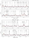 |
Fig. C.2 Same as Fig. C.1 but now for S68N. |
| In the text | |
|
Fig. C.2 continued. |
| In the text | |
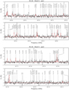 |
Fig. C.3 Same as Fig. C.1 but now for B1-bS. |
| In the text | |
|
Fig. C.3 continued. |
| In the text | |
|
Fig. D.1 Full Band 3 spectrum of B1-c (black) with best fitting CASSIS model overplotted (red). We indicate the positions of species, where lines in italic are excluded in the fitting. |
| In the text | |
|
Fig. D.1 continued. |
| In the text | |
|
Fig. D.1 continued. |
| In the text | |
|
Fig. D.1 continued. |
| In the text | |
Current usage metrics show cumulative count of Article Views (full-text article views including HTML views, PDF and ePub downloads, according to the available data) and Abstracts Views on Vision4Press platform.
Data correspond to usage on the plateform after 2015. The current usage metrics is available 48-96 hours after online publication and is updated daily on week days.
Initial download of the metrics may take a while.