| Issue |
A&A
Volume 639, July 2020
|
|
|---|---|---|
| Article Number | A19 | |
| Number of page(s) | 12 | |
| Section | The Sun and the Heliosphere | |
| DOI | https://doi.org/10.1051/0004-6361/201936762 | |
| Published online | 02 July 2020 | |
High-resolution spectroscopy of a surge in an emerging flux region⋆
1
Leibniz-Institut für Astrophysik Potsdam (AIP), An der Sternwarte 16, 14482 Potsdam, Germany
e-mail: This email address is being protected from spambots. You need JavaScript enabled to view it.
2
Universität Potsdam, Institut für Physik und Astronomie, Karl-Liebknecht-Straße 24 – 25, 14476 Potsdam, Germany
3
University of Delhi, Bhaskaracharya College of Applied Sciences, Sector 2, Phase 1, Dwarka, New Delhi 110075, India
4
Astronomical Institute of the Czech Academy of Sciences, Fričova 298, 25165 Ondřejov, Czech Republic
Received:
23
September
2019
Accepted:
7
May
2020
Abstract
Aims. The regular pattern of quiet-Sun magnetic fields was disturbed by newly emerging magnetic flux, which led a day later to two homologous surges after renewed flux emergence, affecting all atmospheric layers. Hence, simultaneous observations in different atmospheric heights are needed to understand the interaction of rising flux tubes with the surrounding plasma, in particular by exploiting the important diagnostic capabilities provided by the strong chromospheric Hα line regarding morphology and energetic processes in active regions.
Methods. A newly emerged active region NOAA 12722 was observed with the Vacuum Tower Telescope (VTT) at Observatorio del Teide, Tenerife, Spain, on 11 September 2018. High spectral resolution observations using the echelle spectrograph in the chromospheric Hαλ6562.8 Å line were obtained in the early growth phase. Noise-stripped Hα line profiles yield maps of line-core and bisector velocities, which were contrasted with velocities inferred from Cloud Model inversions. A high-resolution imaging system recorded simultaneously broad- and narrowband Hα context images. The Solar Dynamics Observatory provided additional continuum images, line-of-sight (LOS) magnetograms, and UV and extreme UV (EUV) images, which link the different solar atmospheric layers.
Results. The active region started as a bipolar region with continuous flux emergence when a new flux system emerged in the leading part during the VTT observations, resulting in two homologous surges. While flux cancellation at the base of the surges provided the energy for ejecting the cool plasma, strong proper motions of the leading pores changed the magnetic field topology making the region susceptible to surging. Despite the surge activity in the leading part, an arch filament system in the trailing part of the old flux remained stable. Thus, stable and violently expelled mass-loaded ascending magnetic structures can coexist in close proximity. Investigating the height dependence of LOS velocities revealed the existence of neighboring strong up- and downflows. However, downflows occur with a time lag. The opacity of the ejected cool plasma decreases with distance from the base of the surge, while the speed of the ejecta increases. The location at which the surge becomes invisible in Hα corresponds to the interface where the surge brightens in He IIλ304 Å. Broad-shouldered and dual-lobed Hα profiles suggests accelerated or decelerated and highly structured LOS plasma flows. Significantly broadened Hα profiles imply significant heating at the base of the surges, which is also supported by bright kernels in UV and EUV images uncovered by swaying motions of dark fibrils at the base of the surges.
Conclusions. The interaction of newly emerging flux with pre-existing flux concentrations of a young, diffuse active region provided suitable conditions for two homologous surges. High-resolution spectroscopy revealed broadened and dual-lobed Hα profiles tracing accelerated or decelerated flows of cool plasma along the multi-threaded structure of the surge.
Key words: Sun: activity / Sun: chromosphere / Sun: photosphere / line: profiles / methods: observational
Movies are available at https://www.aanda.org
© ESO 2020
1. Introduction
The chromosphere is a very dynamic layer of the solar atmosphere that displays various fine structures on different spatial and temporal scales (e.g., Beckers 1964; Bray & Loughhead 1974). A surge is a chromospheric eruptive feature visible in the blue and red wings of the Hα line where cool plasma is ejected. The first surge observations were reported in the early 1940s (e.g., Newton 1942; Ellison 1942). Since then, various properties of Hα surges have been at the focus of many studies. Apart from Hα, surges are visible in other chromospheric lines, for example in He II 304 Å (Georgakilas et al. 1999), Hβ (Zhang et al. 2000), Ca II H (Tziotziou et al. 2005), C IV, and several UV and extreme UV (EUV) lines (e.g., Liu & Kurokawa 2004; Kayshap et al. 2013).
Bruzek et al. (1974) explained surges as curved or straight spikes of material shooting out and reaching coronal heights at velocities of up to 200 km s−1 with a lifetime of 10–20 min. The surge material usually appears in absorption on the solar disk. Roy (1973a) suggested that surges share properties with prominences, where material is supported by the strong magnetic fields above active regions. Roy (1973b) noted that surges are expected in the proximity of spots or pores with small-scale flares or brightenings such as Ellerman bombs (Ellerman 1917). In addition, regions with evolving magnetic features, that is most notably emerging flux regions (EFRs), are more likely to have surges. Roy (1973a) found that the velocity curve for surges begins with material being accelerated to maximum velocity, and then decelerates under the influence of the magnetic field supporting the surge.
Magnetic reconnection was proposed by Yokoyama & Shibata (1995) as the origin of Hα surges. In their simulations, the whip-like motion of cool chromospheric plasma is produced because of reconnection in an EFR. When the cool plasma is carried to higher atmospheric layers by the expanding flux loops, reconnection in these loops produces a slingshot-like motion, which they associated with Hα surges. Small-scale magnetic features and their association with surges were the focus of the investigation by Brooks et al. (2007), who linked flux cancellation in an emerging flux region to surges. Slow reconnection related to flux cancellation was identified by Chae et al. (1999) as the cause of a surge, where the ejection of cool and hot plasma along different magnetic field lines leads to signatures in Hα and EUV lines, respectively. The base of surges and kernels of UV brightenings are often located near magnetic neutral lines, where opposite-polarity features collide (Yoshimura et al. 2003).
Spectral observations of surges were presented in many studies, for example Schmieder et al. (1983) selected the Hα and C IV lines for their observations. Hα showed lower acceleration, and a shock wave appeared in the upper part of the surge. Schmieder et al. (1994) addressed the question of what mechanism is responsible for driving the surge and maintaining the cool plasma ejection. By comparing two transient events in the same active region, they explored the ejection mechanism, and suggested that just a pressure-driven mechanism is insufficient to explain the properties of the ejected material. Madjarska et al. (2009) discussed trigger mechanisms of a surge using filtergrams taken at five positions along the Hα line. The observed surge seemed to be triggered by an Ellerman bomb. The authors emphasized the need for high spatial resolution and high spectral resolution to disentangle the various chromospheric phenomena.
Nóbrega-Siverio et al. (2016) presented numerical modeling of a surge and performed a 2.5D numerical experiment describing the emergence of magnetized plasma from lower atmospheric layers to the corona. They considered entropy sources, which allowed them to trace the evolutionary pattern of the plasma elements in the surge. They concluded that entropy sources are essential to understand thermal properties of surges. Combining radiation transfer (Bifrost, Gudiksen et al. 2011) and extensive Lagrange tracing, they identified four different populations in the surge. One population covers 34% of the surge’s cross section and reaches temperatures as high as 106 K, which however returns to typical surge temperatures of 104 K by radiative losses and thermal conduction. This suggests that heating and cooling processes are important aspects of the surging plasma. In Nóbrega-Siverio et al. (2017, 2018), they extended the numerical experiments to Si IV and O IV lines to understand the flow of material and energy in the transition region.
The strong absorption line Hα provides access to the thermal and dynamic properties of chromospheric features. For example, Verma et al. (2012) used high-resolution Hα spectra in combination with data of the Japanese Hinode space mission (Kosugi et al. 2007) to study the slow decay of two spots over five days, and Kuckein et al. (2016) studied a large quiet-Sun filament using similar Hα spectroscopic data. The potential of a dedicated data pipeline for the bulk-processing of Hα spectra is presented in Dineva et al. (2020), where noise-stripping based on principal component analysis (PCA) prepares Hα contrast profiles for cloud model (CM, Beckers 1964) inversions.
In the present work we follow the evolution of an EFR with strong absorption features in proximity to sites of continuous flux emergence. In Sect. 2, we present the observations and the various steps to process the data. In Sect. 3, we introduce slit-reconstructed intensity and velocity maps and describe the temporal and spatial variation in Hα line profiles that are associated with the two homologous surges. In addition, we discuss the magnetic field evolution and the response of the upper atmosphere. Our results are discussed in Sect. 4 and placed in the context of relevant literature related to surges and other ejecta. The high spectral and good spatial resolution of the Vacuum Tower Telescope (VTT, von der Lühe 1998) echelle spectrograph were the point of departure for this work and allowed us to investigate the complex evolution and dynamics of the strong absorption features for almost four hours, thus adding to the still sparse knowledge of the spectral characteristics of surges. Future work and prospects for high-cadence scans with the VTT echelle spectrograph are described in our concluding remarks in Sect. 5.
2. Observations and data reduction
The spectroscopic data covering active region NOAA 12722 were acquired at the VTT on 11 September 2018. In total 20 scans were taken in three spectral lines between 08:05 UT and 11:49 UT, describing the evolution of the active region. During this time period of about 3.5 hours, only two gaps of 20 and 17 min occurred between scans 9 & 10 and 15 & 16, respectively. Five sets of flat-field frames with 200 scan steps were recorded at solar disk center while changing the telescope pointing following a circular track. The average dark frame was computed from 200 individual frames.
The spectral lines Hαλ6562.8 Å, Cr Iλ5781 Å, and Hβλ4861 Å were simultaneously recorded with the VTT echelle spectrograph by utilizing the chromospheric grating with a blaze angle of 62°. Even though all three spectral lines were processed, the present study focuses solely on Hα spectroscopy. The slit width was 80 μm, resulting in an exposure time of 300 ms, which matches the full-well capacity of the detector. A broadband interference filter with a full width at half maximum (FWHM) of 8.7 Å and with a peak transmission of 62% was used to suppress overlapping spectral orders. The pco.4000 CCD camera has a quantum efficiency of about 30–40% in the spectral range of 4000–6500 Å. After 2 × 2-pixel binning and discarding the borders, the spectra have a size of 2000 × 660 pixels. The pixel size of the CCD detectors is 9 μm × 9 μm. The resulting pixel size on the solar surface is about 0.18″in the slit direction. The scan step size is 0.16″, and 630 scan steps are recorded, scanning a range of ±50″around the lock point of the Kiepenheuer Adaptive Optics System (KAOS, von der Lühe et al. 2003). This scan sequence takes about 9 min and results in slit-reconstructed maps with a size of 100″× 120″ for the physical parameters derived from the spectral profiles. The dispersion is about 4.2 mÅ pixel−1, and the spectral range covered by the detector is about 8.4 Å.
The spectral data went through the usual preprocessing steps, which includes dark subtraction, flat-fielding, removal of the spectrograph profiles. Noise is removed from the Hα spectra using PCA, and CM inversions are computed for all the 20 scans. The details of the pre-processing steps and CM inversions are presented in Dineva et al. (2020), who used iterative PCA for dimensionality reduction, resorting to only ten eigenfunctions, which represent the Hα spectral line. The resulting spectra are resampled to only 601 wavelength points, which cover a wavelength region of ±3 Å around the Hα line core. The coarser dispersion of 10 mÅ pixel−1 significantly reduced the computation time for CM inversions and PCA decomposition. The final results are noise-free spectra and maps of physical parameters computed using these profiles. An example comparing observed intensity and contrast profiles with the noise-free spectra is compiled in Fig. 7 of Dineva et al. (2020). The CM inversions delivered four physical parameters: optical thickness τ, Doppler width ΔλD, line-of-sight (LOS) velocity of the cloud material vD, and source function S.
As an alternative to observations with the echelle spectrograph, a system of two synchronized LaVision Imager M-lite 2M CMOS cameras were used to capture narrow- and broadband Hα filtergrams. The narrowband filtergrams were obtained with a Lyot filter (λ6562.8 Å and Δλ = 0.60 Å) manufactured by Bernhard Halle Nachf., Berlin-Steglitz (Künzel 1955), and the broadband filtergrams were captured with an interference filter (λ6567 Å and Δλ = 7.5 Å). The details about the setup and data processing are given in Denker et al. (2020). We note that these images were not simultaneously taken with spectral data, but earlier at 07:50 UT. Here, the restored narrow- and broadband filtergrams serve as high-resolution context images. Images were restored using Multi-Object Multi-Frame Blind Deconvolution (MOMFBD, van Noort et al. 2005).
The Solar Dynamics Observatory (SDO, Pesnell et al. 2012) provided full-disk context images and magnetograms used to discuss the temporal evolution and morphology of the active region. The continuum images and LOS magnetograms were obtained with the Helioseismic and Magnetic Imager (HMI, Scherrer et al. 2012), whereas the Atmospheric Imaging Assembly (AIA, Lemen et al. 2012) provided UV λ1600 Å and EUV He IIλ304 Å images. These two wavelengths cover different layers in solar atmosphere with about 430 km (Fossum & Carlsson 2005) and about 4000 km (Alissandrakis 2019) as formation heights, respectively. Data processing follows the steps outlined in Beauregard et al. (2012) and Verma (2018).
3. Results
Active region NOAA 12722 appeared on the solar surface at around 19:00 UT on 10 September 2018. By the time of the VTT observations on 11 September 2018, the region (see Fig. 1) was located at disk-center coordinates (440″ E, 210″ S), which correspond to a cosine of the heliocentric angle of μ ≈ 0.86. The full field of view (FOV) covered by the scans with the VTT echelle spectrograph was cropped to 100″ × 100″ as indicated by the black and white boxes in Fig. 1. A corresponding movie with the detailed view of the central 100″ × 100″ is available online. Since AIA and HMI data are recorded at different cadences from 12 s to 45 s, the time series were resampled to a one-minute cadence covering the period 07:30–12:00 UT. For this purpose, the time series were corrected for solar differential rotation before using linear interpolation to an equidistant grid in time on a pixel-by-pixel basis. The restricted FOV presented in the top panels of Fig. 2 is used in the following for the investigation of the surges.
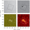 |
Fig. 1. Overview of active region NOAA 12722: HMI continuum image (top left), HMI magnetogram (top right), AIA UV λ1600 Å image (bottom left), and AIA EUV He IIλ304 Å image (bottom right) observed at 08:05 UT on 11 September 2018. The magnetogram was clipped between ±250 G. The black and white boxes represent the central 100″ × 100″ of the FOV scanned by the VTT echelle spectrograph (see online movie with a one-minute cadence for a detailed view). |
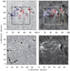 |
Fig. 2. Slit-reconstructed Hα continuum (top left) and line-core (top right) intensity images of active region NOAA 12722 observed at 08:05 UT on 11 September 2018. The blue and red contours refer to a co-temporal magnetogram at ±100, ±250, and ±500 G. The black and white squares give the location of restored Hα broadband (bottom left) and narrowband line-core (bottom right) filtergrams taken at 07:50 UT. The yellow rectangle (top right) gives the location of continuous surge activity. |
In the next sections we describe first the magnetic field evolution and response of the upper atmosphere based on the time series of SDO data, and then we study various line properties extracted from the noise-free Hα spectra. The morphology of absorption features was derived from slit-reconstructed red and blue wing maps and from the line-core maps. Time series of matching LOS velocity maps reveal the dynamics of the surge, while selected Hα line profiles allow us to describe their complex spatio-temporal properties.
3.1. Magnetic field evolution
The active region emerged with the trailing negative polarity being more prominent with two tiny pores and a very dispersed leading positive polarity, which deviates from the typical emergence pattern of active regions. Tiny pores of positive polarity appeared at around 05:00 UT on 11 September 2018. In addition, a new flux system with mixed polarity started to emerge in the leading part of the already existing region at around 06:00 UT. When the VTT observations started at 08:05 UT, the region consisted of multiple pores with continuous flux emergence in the leading region as shown in Fig. 1. In Fig. 2, the slit-reconstructed continuum and line-core maps from the first scan are displayed with contours of a magnetogram taken at the same time. The pores belong to the already existing system with flux emergence in the trailing part and are labeled P1, P2 and N1, N2 for positive and negative polarities, respectively. The pores associated with the new flux system are labeled by p1, p2, and n1, referring again to positive and negative polarities. Several other features with mixed polarities are not discretely tagged.
The restored high-resolution images from the CMOS cameras show diffraction-limited details of the photosphere and chromosphere (bottom panels of Fig. 2). Elongated granules between pores P1 and N2 indicate ongoing flux emergence (e.g., Verma et al. 2016). In addition, the Hα broadband image and the time series of HMI continuum images show both indications of thread-like dark intergranular lanes connecting opposite magnetic polarities (e.g., Strous et al. 1996), which are a signature of emerging Ω-loops capable of lifting cool plasma into higher atmospheric layers. As a result, a typical arch filament system (AFS, e.g., González Manrique et al. 2018) is evident in the Hα narrowband filtergram between these pores. In general, the pre-existing flux in the trailing bipolar region evolves gradually, leading to a simplification and stretching of the active region in the trailing part over time.
In contrast, the newly emerging flux system exhibits strong upwelling flux to the north between pores P2 and p1 in form of small-scale negative-polarity features resembling type III moving magnetic features (MMFs, Kubo et al. 2007), but in absence of a moat region around the pores. The observed enhanced Hα line-wing and line-core emission (i.e., bright Hα grains) may be signatures of reconnection events of undulating, serpentine field lines that rise up in the atmosphere as mass-loaded U-loops (Pariat et al. 2004). These bright Hα grains coincided with UV brightenings similar to UV bursts, which were associated by Ortiz et al. (2020) with Ellerman bombs and emerging flux. Strengthening of pores p1 and p2 balances the flux emergence. The significant growth and strong proper motion towards the west of pore p2 impacts the magnetic field topology of the active region and is, in addition to flux cancellation, an ingredient of surging. The base of the surge is associated with the negative-polarity feature n1 in the western part of the region but not exactly at the periphery (cf., Mulay et al. 2016). Continuous flux cancellation occurs during the 3 1/2-hour period covered by the SDO HMI/AIA movie. The cool plasma was ejected towards the south, but the exact orientation of the surges was difficult to determine because the region is not located at the solar disk center, and it appears as if the material is not ejected radially. Thus, the LOS velocities computed in later sections may underestimate the speed of the ejected plasma. The broad surge-like structure is shown by the yellow rectangle in the upper panel of Fig. 2.
3.2. Response of the upper atmosphere
In this section we discuss the response of the upper atmosphere of the surge activity using the online movie accompanying Fig. 1. The first indication of surge activity is already visible at the location of the canceling magnetic feature n1 in AIA UV and EUV images at around 08:37 UT. The UV images show a confined brightening of two small kernels, and the EUV intensity lags by about one minute and reaches its peak brightening at around 08:40 UT. The EUV brightenings are more structured and cover a larger area. These UV and EUV brightenings are indicative of localized heating in the lower atmosphere. In the EUV images a surge appears around this time, first as a dark structure; it then brightens, including a thin collimated bright structure, as the surge progresses. The surge continues beyond the southern edge of the FOV (at around 08:44 UT) in the online movie belonging to Fig. 1. In the UV images, this surge appears only as faint hazy bright structure in proximity to the negative-polarity feature n1.
Starting around 09:05 UT, UV and EUV brightenings appear in the neighborhood of the negative-polarity feature n1. They are not always visible in the EUV images, where they are often obscured by opaque dark filaments higher up. However, the swaying motion of the filaments uncover these brightenings from time to time, indicating that the heating observed in the UV and EUV images occurs below the filamentary structure. The second major surge starts at around 09:17 UT with a homologous appearance and propagation pattern as its precursor, however, affecting a much larger area with respect to brightenings and ejected material. Even the AFS in the trailing part of the active region is affected; that is, the loop system connecting opposite polarities is activated and significantly brightens. Again, opaque material jutting out to the south from the base of the surge becomes brighter and less opaque while being ejected, which is evident in the EUV images at around 09:36 UT. After this time some ejected material returns, and both bright loops and dark filaments exhibit complex and dynamic interactions until the end of the SDO HMI/AIA movie at 12:00 UT.
Reconnection at the cancellation site provides the energy for propelling the surging cool plasma. Proper motions and shear are important ingredients to store energy in non-potential magnetic field configurations. In addition, they can open or stretch the overarching magnetic field loops allowing the plasma to escape. The role of shear flows and other types of proper motions has recently attracted renewed interest in the context of surges (e.g., Yang et al. 2019). The background-subtracted activity maps (BaSAMs, Denker & Verma 2019) in Fig. 3 highlight locations in the active region with strong variations of the magnetic field and UV intensity. Continued flux emergence is clearly evident in the trailing bipolar part of the active region but also cancellation near the negative-polarity feature n1. Growth of both pores p1 and p2 leaves a strong signature in the magnetic BaSAM, which is enhanced by the strong proper motions of pore p2. The UV intensity variation caused by intermittent bightenings shows a strong disparity between the pre-existing flux system in the trailing part and the very dynamically evolving leading part of the active region. Several kernels of enhanced UV variation are visible near the negative-polarity feature n1 and in the “wake” of the fast moving pore p2.
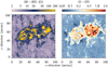 |
Fig. 3. Background-subtracted activity maps of the LOS magnetic field B (left) and the UV λ1600 nm intensity I (right). The maps were computed for the time period 07:30–12:00 UT and show the locations with strong variations of the magnetic field and UV intensity. The black plus sign (+) and cross (×) indicate the location of persistent blue- and redshifted regions as discussed in Sect. 3.5 and depicted in Fig. 5. The labels in the right panel are the same as in Fig. 2. |
3.3. Temporal evolution in Hα line-wing and line-core maps
Blue and red line-wing maps along with line-core maps were created (Fig. 4) to investigate the evolution of the active region in different atmospheric heights. The Hα line-wing maps were obtained at ±1.0 Å from the central line-core position. All three parameters are also compiled in an online movie where the ongoing dynamics in the region can be visualized.
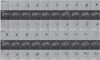 |
Fig. 4. Slit-reconstructed Hα line-core intensity maps (rows 2 and 5) for all 20 scans, along with the corresponding maps of the blue (rows 1 and 4) and red (rows 3 and 6) line-wing intensity at ±1.0 Å observed on 11 September 2018. The image contrast of the line-core, and blue and red line-wing intensity maps are in the ranges 0.15–0.80, 0.25–1.4, and 0.25–1.4 I/I0, respectively. All maps depict the region of interest of 100″ × 100″shown in the top panels of Fig. 2. Two locations along the surge are indicated in panel seven of row 2 as S1 and S2, which are discussed in Sect. 3.6 and depicted in Fig. 10. The accompanying online movie furnishes a detailed view of ongoing dynamics in the active region. |
In the first two scans, contrast features appear at small scales. The blueshifted absorption features are more concentrated in the newly emerging region. The location of these features coincides with the mixed-polarity region. By the third and fourth scan at 08:24 and 08:34 UT, respectively, these absorption features become more elongated in the blue wing, which leads up to the first smaller surge. However, small-scale counterparts in the red wing remain faint. Starting with the fifth scan at 08:43 UT, extended absorption features appear in the red wing between pore p1 and the negative-polarity feature n1. The second stronger surge at 09:05 UT leads to darker absorption features at the same location, which only fade after 09:52 UT. By this time the features in the red wing are elongated and located just next to the blue-wing features. The absorption features in the blue wing slowly disappear and by the end of a scan at 11:49 UT, only very faint signatures are left, whereas the red-wing features persist and trace out a bright oval structure in the line-core intensity maps. In general, absorption features in the red wing appear later than in the blue wing. This agrees with the findings of Yang et al. (2019) who observed that blueshifts occur first but that the phase of redshifts persists longer. We note that the scans take about 9 min, which has to be taken into account when comparing slit-reconstructed VTT data to more instantaneous SDO imaging and magnetogram data. However, certain locations in the slit-reconstructed data can be dated more precisely depending on the number of covered slit positions (i.e., 70 slit positions or about 11″ are covered in one minute). In this time interval about three matching He IIλ304 Å images are available. Considering these limitations, it can be concluded that the surges appear simultaneously in Hα and He IIλ304 Å.
The two homologous surges, appearing in the line-core maps at 08:34 UT and 09:05 UT, were observed in the newly emerging region with mixed polarities. The surging activity lasted longer (more than 90 min) compared to typical Hα surges, which are rather short-lived. The second stronger surge extended for about 28″and was about 12″wide. It is not a uniform absorption feature, but exhibits substructures with a width of 4–8″. The multi-threaded morphology of surges can be explained by simulations of chromospheric ejecta along twisted magnetic field lines by Iijima & Yokoyama (2017). In addition, the later stages of the active region evolution is dominated by downward drainage of plasma. Furthermore, small-scale brightenings are continuously present in line-core, blue-wing, and red-wing maps. They are related to bright Hα grains caused by strong-field magnetic concentrations (MCs, Rutten et al. 2013), which are associated with the upwelling magnetic flux between pores P2 and p1 (see Sect. 3.1). Only resolved spectra can reveal the differences between bright Hα grains and Ellerman bombs, where in the latter case the line-core intensity is not enhanced. Thus, misclassification may be an issue in studies resorting to Hα filtergrams. Considering the dynamic flux emergence, Ellerman bombs and bright Hα grains are likely associated with photospheric reconnection leading to surges. Surges and Ellerman bombs, and also bright Hα grains, can occur together but not exclusively (e.g., Watanabe et al. 2011). However, the nature of continuously evolving small-scale mixed polarities and their ambiguous relationship to brightenings at various atmospheric heights hamper a clear causation among various features, at least in crowded and complex magnetic environments.
3.4. Line-of-sight velocities
The detailed inspection of absorption features in the red and blue wings is based on LOS velocity maps for the line core for all 20 scans. The line-core velocities are estimated by first finding the minimum of the Hα line-core intensity and its position, followed by fitting a range of ±0.3 Å around this location with a parabola. Thus, the line-core velocity can be determined across almost the entire spectral range covered by the detector. In addition, similar maps of the bisector velocity corresponding to the FWHM of the Hα line profile provide information of plasma motions lower in the atmosphere. The FWHM and the corresponding velocity were determined individually for each profile between minimum and maximum intensity in the observed spectral range of ±3 Å. The maximum intensity is almost the same in all cases (Imax ≈ 0.85 I0) as a result of normalizing the spectra to the quiet-Sun continuum intensity.
According to Vernazza et al. (1973), the Hα line is formed at about 300–1600 km in the atmosphere. As is widely accepted, the line core originates higher in the chromosphere than the line wings (Cauzzi et al. 2009). Accurate calculations of the Hα formation height are provided by Leenaarts et al. (2006). In their detailed work regarding the formation of the Hα line, Leenaarts et al. (2012) found that the Hα line-core intensity is correlated with the average formation height; that is, the intensity decreases with increasing formation height. Nevertheless, pinpointing the exact formation height of Hα remains elusive. Maps of the FWHM and line-core velocity are compared in Fig. 5, where velocities are scaled between ±10 km s−1, and red- and blueshifts (down- and upflows) are displayed in white and black, respectively. Noise-free spectral profiles after PCA decomposition and without the contamination of line blends helped in creating these maps. The changes in these two parameters can also be visualized in the accompanying online movie.
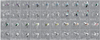 |
Fig. 5. Slit-reconstructed FWHM (rows 1 and 3) and line-core (rows 2 and 4) velocity maps. The maps are scaled between ±10 km s−1. Black and white corresponds to upflows and downflows, respectively. The colored plus signs (+) and crosses (×) are persistent blue- and redshifted regions recognized by using the average of 20 velocity maps with LOS velocities of ±3 km s−1. The corresponding Hα profiles are shown in Fig. 6. The intensity and contrast profiles along the green lines in panels 7 – 9 are displayed in Fig. 8. The accompanying online movie provides a visualization of the temporal changes of these two parameters. |
At first glance the velocity pattern at both heights appears to be similar. However, closer inspection reveals more details in the line-core maps. The most conspicuous changes of the LOS velocities are located in the leading part of the active region, where magnetic flux continuously emerges, as is evident in all 20 scans. Flux emergence is accompanied with small patches of downflows between the leading and trailing pores P2, p1, p2, and n1. By the second scan, additional small upflow patches materialize in proximity to these downflow patches, which are most prominent around the leading pores p1 and p2. The velocity pattern associated with the region of continuous flux emergence between the pore p1 and the negative-polarity feature n1 is discussed in more detail below.
Major differences start to show up in the third scan at 08:24 UT leading up to the first surge. A fan-shaped region with strong downflows in the center of the FOV and a small elongated upflow region become visible in the line-core velocity map in the middle of the new flux system, that is between pore p1 and the negative-polarity feature n1. However, in the FWHM velocity map, the upflow region is more prominent and extended, which indicates upward-moving plasma that has not yet reached the formation height of the line core. Ten minutes later, a small fan-like structure forms but with patches of down- and upflows. The upflow patches now become conspicuous. The velocity pattern is again changed by the fifth scan at 08:43 UT at the location of the first surge. The fan-like structure around the mixed polarity region is now replaced by a V-shaped feature, where the arms indicate locations of downflow with small adjacent upflow patches. The pattern of the FWHM velocity is similar to that of the line core, but downflows are much weaker.
Strong absorption features (Fig. 4) appear in the scans after 09:05 UT signalling the initiation of the second surge. In the velocity maps (Fig. 5), an upflow patch in the line-core velocity map is followed by a downflow patch and then by another upflow patch along the green line, which is plotted in three panels starting at 09:05 UT. This upflow patch is more prominent at the formation height corresponding to the FWHM. At 09:14 UT, the upflow patch is more extended and elongated in both the line-core and FWHM velocity maps. At this point, the surge reaches its maximum expansion. The pattern remains the same for the next scan with a strong upflow patch. For the next scans, patches with strong downflows appear. However, in the FWHM velocity map, the upflow patch persists and is accompanied by a downflow patch.
3.5. Evolution in the temporal and spatial domains
The average Hα profiles were plotted for all 20 scans in Fig. 6 to illustrate the variety of down- and upflows in the surging region. The black profile in the panels refers to the average quiet-Sun profile. Noise was significantly reduced in the Hα profiles using PCA decomposition, which also facilitated the removal of telluric and solar line blends. The locations of persistent down- and upflows were chosen from the average LOS velocity map and by applying a lower threshold of 3 km s−1 to the flow speed. Two small 10 × 10 pixel regions were selected in the mixed polarity region. In addition, these locations are associated with flux cancellation near the negative-polarity feature n1 and the strong proper motion of pore p2, as is evident from the BaSAMs (see Fig. 3). Downflows are initially located at pore p2, which is responsible for changing the magnetic field topology, whereas upflows coincide with the negative-polarity feature n1, which is directly associated with the surge activity. These 10 × 10 pixel regions are indicated in Figs. 3 and 5 by plus signs (+) and crosses (×) referring to locations of persistent down- and upflows, respectively.
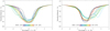 |
Fig. 6. Hα profiles after PCA decomposition for two regions with persistent upflows (left) and downflows (right) in excess of ±3 km s−1 (see online movie with an animated sequence of profiles). The locations are indicated in Fig. 4 by colored plus signs (+) and crosses (×). The color bar at the bottom uses the same color scheme to track the temporal evolution of the spectral line profiles. The black line corresponds to the quiet-Sun profile in both panels. |
Significant changes are seen in the profiles belonging to these two small regions. Blueshifted profiles (left panel in Fig. 6) are slightly displaced for the first two scans, but much less in comparison to shifts for later scans. The line core is deeper compared to an average quiet-Sun line profile. Starting with the third scan, the profiles become shallower and the line-core intensities reach almost I/I0 = 0.3 at the onset of the first surge. In the initial phase of the second surge from 09:05–09:23 UT, the blue-green profiles are shifted up to −1 Å implying Doppler velocities of about 45 km s−1. Double-lobed profiles and profiles with extended shoulders indicate more complex plasma motions either because of features with different Doppler velocities in the same resolution element or because of height-dependent flows. Typically, fast and slow flow components are present in double-lobed profiles. During the time period 09:52–10:10 UT (green) in the later stages of the second surge, the blueshifts reach up to −2Å with corresponding plasma velocities of about 90 km s−1. Thus, the second surge is most clearly visible for a period of about one hour after 09:05 UT. After this the blueshifted profiles slowly reach quiet-Sun line-core intensities but remain broadened, which indicates turbulent and/or heated plasma. The Hα line is an important diagnostic to probe the solar chromosphere (Carlsson et al. 2019). However, the low atomic weight of hydrogen leads to large thermal broadening. Hence, the changes in the Hα line widths are indicative of the temperature changes in the deep photosphere (Cauzzi et al. 2009), whereas changes in line-core intensity indicate variations of the formation height (Leenaarts et al. 2012) because of strong scattering and the sensitivity of irradiation from the surrounding environment.
Redshifted profiles follow the same trend as blueshifted profiles. However, they are always shallower and never reach the quiet-Sun line-core intensity. Furthermore, profiles in the later stages of evolution exhibit enhanced line wings. Line profiles are narrow in the first scan at 08:05 UT, but this changes rapidly in the next scans with the onset of the first surge, when the line profiles become broader and reveal a distinct shoulder in the red wing, which extends to +1 Å and beyond. The profiles during the intervening time interval from 08:43–09:05 UT (i.e., between the two surges) are very broad and shallow. The shoulder reaches almost 2 Å for the scans at 09:14 UT and 09:23 UT once the second surge starts. These profiles even show a clearly separated second lobe and appear at the same time in proximity to the surge. The initially redshifted profiles also return to quiet-Sun conditions towards the end of the observations. The changes in individual profiles can be visualized in the animated online version of Fig. 6.
To quantify the morphological diversity and the trend in the temporal evolution of spectral line profiles, a box and whisker plot (Fig. 7) is created of the FWHM velocities for the locations shown in Fig. 5. The FWHM is chosen to take into consideration the complete line (asymmetric) profile rather than just the line core, which may not be representative for strongly asymmetric profiles. In general, velocities for the satellite component of double-lobed profiles cannot be appropriately derived by bisector analysis. The 10 × 10 pixel regions are used to compute statistical properties such as the mean, standard deviation, median, maximum, and minimum velocity values, which are depicted as center and height of the box, white horizontal line, upper whisker, and lower whisker, respectively. In the early scans at 08:05–08:34 UT, velocities at locations of persistent up- and downflows are insignificant and show little variation. Starting at 08:43 UT, the speeds at both locations start to rise, reaching a maximum of up to ±20 km s−1. The up- and downflow velocities are synchronized and consistently increase until 10:01 UT.
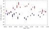 |
Fig. 7. Box and whisker plot of the FWHM velocities at the locations that are indicated in Fig. 5 by colored plus signs (+) and crosses (×). The box extends over one standard deviation above and below the mean velocity of a 10 × 10 pixel region. The upper and lower whisker refer to the maximum and minimum velocity in that region, respectively. Blue and red refer to the location of persistent up- and downflows, respectively. The white horizontal line inside the boxes corresponds to the median velocity. |
Three cross sections along the second surge reveal the spatial variation of the Hα intensity and contrast profiles at 09:05 UT, 09:14 UT, and 09:23 UT, respectively. The displayed contrast profiles refer to (I − I0)/I0, where I0 is the quiet-Sun intensity. The extracted profiles are collected in Fig. 8, which contains 256 profiles in each panel along the cross sections shown in Fig. 5. The profiles in Fig. 8 follow a color scheme from blue to red, which indicates their location along the cross section. The ends of the cross section are indicated by blue and red squares in Fig. 5. The intensity and contrast profiles vary significantly along the cross section. The three scans cover three different stages of the surge. The second surge appears at the bottom of the cross section at 09:05 UT and expands within 20 min to the south. The upper end of the cross section extends towards a quiet-Sun region, whereas the middle part passes through a redshifted region.
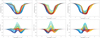 |
Fig. 8. Hα intensity (top) and contrast (bottom) along the green cross section in Fig. 5, which starts at the blue and ends at the red square (see online movie with an animated sequence of profiles). Blue and red also indicate the start and end of the color table for the profiles at 09:05 UT, 09:14 UT, and 09:23 UT (left to right). |
The intensity and contrast profiles are significantly broadened and blueshifted at 09:05 UT at the start of the cross section, as indicated by the dark blue to light blue profiles in the left panel of Fig. 8. Their line-core intensities are initially lower compared to a quiet-Sun profile, but the profiles become rapidly shallower, as is evident from the contrast profiles. These profiles belong to the tip of the surge. Hence, profiles corresponding to strong upflows are expected. Profiles from the central part of the cross section are still broad, but they gradually exhibit a second redshifted component. Towards the base of the surge the redshifts increase, signaling strong downflows, and the profiles show enhanced line-wing emissions. The orange and red profiles at the end of the cross section are slightly broadened and redshifted, but in general they resemble quiet-Sun profiles. The profiles closest to the end of the cross section are very good representations of the quiet-Sun. The discussed properties of intensity profiles are reflected in the contrast profiles, which clearly accentuate line depth and width, as well as line asymmetries and Doppler shifts.
For the scan at 09:14 UT, the lower tip of the surge still exhibits blueshifts, but with narrower line profiles. The slight line-wing enhancement is still present in the turquoise profiles. Further along the cross section, redshifted spectral lines are encountered, as indicated by the yellow-orange profiles. A blueshifted absorption region is located at the upper end of the cross section, which is also reflected in the red profiles with two components. The sequence of profiles changes more gradually along the cross section at 09:23 UT. The blue profiles are clearly blueshifted and become redshifted when progressing along the cross section. A line-wing enhancement is not evident for the third cross section. However, some of the blue profiles show a hint of a second component. For better visualization an animated version of Fig. 8 is available online.
Figure 9 summarizes and quantifies the variation of the FWHM velocities along the three cross sections in Fig. 5. The overall variation along the cross sections is similar but with a distinct shift for the third cross section. Strong upflows between −8 and −12 km s−1 are encountered to the south of the base of the second surge near the negative-polarity feature n1 while the cross section comes across downflows of up to 20 km s−1 near the rapidly evolving and migrating pore p2. The end of the cross section is located in a quiet-Sun region.
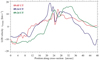 |
Fig. 9. FWHM velocities along the three cross sections in Fig. 5. The zero position corresponds to the blue square and the maximum position to the red square of the cross sections, shown as green lines in Fig. 5. |
3.6. Cloud model inversions
Properties of spectral absorption lines are often more conveniently determined using the contrast profiles. In Fig. 8, contrast profiles along the three cross sections are presented and CM inversions are performed for all 20 scans as mentioned in Sect. 2. The details of CM inversions based on PCA noise-stripped contrast profiles are explained in Dineva et al. (2020). To illustrate the quality of the CM inversions, two examples of PCA decomposed and CM Hα contrast profiles are shown in Fig. 10. The profiles are taken from the two positions in the cross section at 09:05 UT at the onset of the second surge and are labeled S1 and S2 in the line-core map of Fig. 4. Both profiles belong to dark absorption features. However, the optical thickness is higher for S1 with τ0 = 2.25 than for S2 with τ0 = 1.44. The cloud velocity is also higher for S1 with vD = −10.80 km s−1 than for S2 with vD = −8.01 km s−1. In addition, significant line broadening is evident for S1 with ΔλD = 0.89 Å compared to ΔλD = 0.57 Å for S2. Broadened line profiles, strong absorption, and strong upflows thus characterize the site where the surge originates.
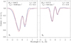 |
Fig. 10. PCA decomposed (solid blue) and CM (dashed red) Hα contrast profiles for two locations S1 (left) and S2 (right) within the surge (see Fig. 4). The CM parameters are given at the top of the panels. |
Two-dimensional maps of the Doppler velocity of the cloud material vD and the optical thickness τ0 are depicted in Fig. 11 for three scans at 09:05 UT, 09:14 UT, and 09:23 UT. We note the deteriorating seeing in the last scan resulting in a washed-out appearance. The three selected scans cover the second surge from onset to roughly its peak and complement the exploration of the three cross sections in Fig. 5. The cloud velocities are significantly higher than those shown in Fig. 9. The CM is based on the assumption that cool absorbing plasma is suspended at chromospheric heights by the magnetic field and that cloud material is irradiated by the photosphere from below and with contributions from the surroundings. The upflows are highly structured and are later accompanied by downflows in close proximity. These simultaneous blue- and redshifts were also noted by Tiwari et al. (2019), but in the IRIS UV spectra. According to these authors the side-by-side up- and downflow of plasma along the surge argues against twisting motions in the surge. The upflows are directed towards the south, but do not reach the southern edge of the FOV. The highest plasma speeds of more than 30 km s−1 are encountered at the leading edge of the surge and are highest at 09:23 UT.
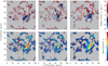 |
Fig. 11. Two-dimensional maps of the inversion results for the two CM parameters based on the noise-stripped contrast profiles for three scans at 09:05 UT, 09:14 UT, and 09:23 UT (left to right): doppler velocity of the cloud material vD (top) and optical thickness τ0 (bottom). The FOV is the same as in Figs. 4 and 5. We note that the velocity of the cloud material vD differs from those depicted in Fig. 5. Regions where the CM is unsuitable and inversions fail are reproduced in gray. |
The optical thickness τ0 is very high at the base of the surge. The high optical thickness in proximity to the base of the surge was also observed by Schmieder et al. (1994). CM inversions, however, fail directly at the base of the surge because of enhanced line-core intensity, which signals local heating of the plasma. This is also supported by the larger Doppler width ΔλD at these locations. The optical thickness decreases in the propagation direction of the surge. At some point the cool plasma becomes either so diluted that only the quiet-Sun photosphere is observed or the ejected plasma is heated to temperatures where Hα becomes ionized. This relatively sharp transition finds its counterpart in the SDO HMI/AIA online movie accompanying Fig. 1; that is, in the EUV λ304 Å time series, the initially opaque dense plasma brightens and can be traced to the edge of the FOV (see Sect. 3.2).
In addition to the surge, a stable arch filament with upflows is present in the left panels of Fig. 11 above the center of the FOV. This points to the complex magnetic structure of the active region. However, it also indicates the co-existence of the old and new flux systems, both of which experience continuous flux emergence. Only in the EUV λ304 Å time series do enhanced brightenings appear in the loop system associated with the arch filament (see Sect. 3.2).
4. Discussion
Surges occur at sites of flux cancellation (i.e., in mixed-polarity regions of an EFR) when trailing and leading parts of the active region separate (Wang & Zirin 1992). Surges are also associated with the cancellation of opposite-polarity MMFs around sunspots at the periphery of the superpenumbra (Wang et al. 1991). In both cases surges feed on the energy supplied by magnetic cancellation and are often accompanied by (sub-)flares, which are, however, absent in the present observations. In the present study flux emergence between the pores P2 and p1 continues throughout the observations, which is accompanied by strong proper motions of pore p2 affecting the magnetic field topology of the active region. Additionally, prolonged flux cancellation occurs near the negative-polarity feature n1, which defines the base of the surge.
Zirin & Werner (1967) reported homologous surges, that is, recurring surges with similar shape and evolution (see also Chen et al. 2008). In the present study two homologous surges were detected during the four-hour observing run, which can be clearly identified when using Hα observations in combination with SDO EUV images. Nelson et al. (2019) suggests that multiple ejections with similar characteristics hint at repetitive drivers, for example, reconnection in the lower atmosphere. However, in the present study, flux cancellation at the negative-polarity feature n1 is continuous rather than repetitive, relaxing the strict requirement of recurrent reconnection. The heating at the base of the surges is noted as continuous brightenings in Hα line-core maps, broad line profiles, and in time-sequence of UV and EUV images as localized brightenings. This is consistent with the established concept that heating in the lower atmosphere pushes plasma higher in the atmosphere during the surge (e.g., Schmieder et al. 1994). Two-dimensional magneto-hydrodynamics simulations by Yang et al. (2018) of a network jet triggered by magnetic reconnection in the transition region during flux emergence show that relatively cool jets are followed by hot fast jets, as observed for surges. The returning plasma of the observed surge does not carry sufficient momentum to disturb the surrounding chromosphere, as was observed by Zirin & Werner (1967), where the impact creates a travelling wave, which in turn caused other surges or flares. In contrast, a regular AFS co-exists undisturbed during the homologous surges. However, the broad Hα spectral profiles near the base of the surge suggest heated and turbulent plasma even in the deep photosphere.
In general, the observed FWHM velocities of about 20 km s−1 are well above the sound speed of about 10 km s−1, but remain at the lower end of values reported in literature: about 30 km s−1 by Chen et al. (2008), 40 km s−1 by Watanabe et al. (2011), 70 km s−1 by Yang et al. (2014), 100 km s−1 by Sánchez-Andrade Nuño et al. (2008), and 200 km s−1 by Bruzek et al. (1974). Even the CM velocities of more than 30 km s−1 remain at the lower end of the cited studies and stay well below the Alfvén speed of about 100 km s−1. Only some of the double-lobed Hα line profiles imply plasma motion reaching the Alfvén speed. In any case, some ambiguity remains depending on the methods that were used to determine the surge velocities: time-space slices, feature tracking, line-core fitting, bisector analysis, CM inversions, or modeling of dual- or multi-component spectral line profiles.
In addition, the complexity of spectral line profiles may not be appropriately captured by imaging spectrometers with lower spectral resolution; for example, only five spectral points were covered in Hα by Madjarska et al. (2009) and 23 in Watanabe et al. (2011). Even in recent studies of Hα surge observation this limitation remains; for example, Yang et al. (2019) used nine wavelength points, Nelson et al. (2019) used 35 wavelength points, and Ortiz et al. (2020) used 15 wavelengths points. Currently, spectroscopic Hα observations are only available from the ground. Thus, even in the presence of real-time adaptive optics correction and image restoration, variable seeing conditions will impact the analysis of spectral profiles. In spectral inversions, these impacts may even be larger than the intrinsic error of the inversion techniques. In the meantime, the Chinese Solar Hα Imaging Spectrometer (SHIS, Chen 2018) spacecraft recently received approval, and Hα spectral data free of seeing influence will be available in the future.
Surges are a common phenomenon in EFRs and sites of flux cancellation. However, investigations of the ejected surge plasma are not frequently carried out using high spectral resolution Hα spectroscopy. The present investigation combines moderate temporal (about 10-min cadence) with good spectral resolution (4.2 mÅ pixel−1 dispersion) and good spatial resolution (better than one second of arc), which allowed us to trace the detailed temporal evolution and spatial variation of a surge. The spatio-temporal properties of the Hα line profiles in Figs. 6 and 8 clearly demonstrate that the velocity distribution along the surge is highly structured and very variable in time. Higher spatial resolution can be achieved with imaging spectrometers such as CRISP (e.g., Scharmer et al. 2008; Watanabe et al. 2011), but with much lower spectral resolution. On the other hand, the Fast Imaging Solar Spectrograph (FISS, Chae et al. 2013) delivers resolved spectral observations in Hα and Ca IIλ8542 Å and provides higher spatial resolution but over a smaller FOV compared to the VTT echelle spectrograph.
5. Conclusions
The aim of the present study was to demonstrate the potential of high-resolution spectroscopy for the investigation of solar eruptive phenomena, specifically two homologous surges in the present case. Resolved line profiles are rare and spectral features are often obscured by resorting to filtergrams and narrowband images. Furthermore, noise in addition to solar and telluric blends affects the analysis of strong chromospheric absorption lines. Improvements in data processing (see Dineva et al. 2020) addressed these issues, and this is the first scientific investigation that benefits from these software tools implemented in the “sTools” IDL software library (Kuckein et al. 2017).
The high-resolution noise-stripped Hα observations in conjunction with SDO LOS magnetograms and UV and EUV images revealed various physical properties of the observed surges. The homologous surges appear in a region of new flux emergence. The interaction of new emerging flux with pre-existing magnetic flux concentrations provides suitable conditions, namely flux cancellation and strong proper motions required for the seen surge activity. The two events of enhanced surge activity are related to the locations of flux cancellation and strong proper motions, which in turn are the locations of persistent side-by-side down- and upflows. Furthermore, the surges associated with the new emerging magnetic flux co-exist with the stable AFS established within the preexisting active region magnetic flux. Broad and dual-lobed Hα profiles are prevalent along the surge, representing accelerated or decelerated flows of cool plasma with complex structure. Additionally, broad Hα profiles indicate enhanced heating at the base of the surge (i.e., strong gradients in temperature and density) where cool plasma in Hα absorption features is located above heated regions. This scenario is also supported by the presence of bright kernels in UV and EUV images. The opacity of the cool surge plasma is estimated using CM inversions. The opacity decreases from the base of the surge to the tip. The decrease in opacity coincides with the increase in the speed of the cloud material. The low excitation energy of 10.2 eV of the Hα transition implies its strong sensitivity to temperature. When cool gas of considerable opacity is propelled to higher atmospheric layers it will dilute and assume higher temperatures. Thus, ionization of neutral hydrogen becomes important. Surprisingly, the location where the surges fade from the Hα observations coincides with the interface where the surge brightens in He IIλ304 Å.
The Hα observations present only a small fraction of the overall data covering the two homologous surges, that is, a detailed analysis of Hα, Hβ, and Cr I spectra along with more advanced CM inversions (see Tsiropoula et al. 2012), and magnetic field information (see, e.g., Del Toro Iniesta & Ruiz Cobo 1996, for Stokes Inversions based on Response functions (SIR) of Stokes-I) will be presented in a forthcoming study. Such an investigation will focus on line formation and peculiar features in spectral lines associated with surging plasma. Multi-line spectroscopy with the VTT echelle spectrograph has the advantage of co-spatial and co-temporal observations, which is beneficial for numerical modelling. The synthesis of spectral lines can thus rely on a broad range of physical parameters describing the magnetic field and plasma flows in the photosphere and chromosphere. The first results presented in Sect. 3.6 illustrate the quality and potential of CM inversions, which facilitated investigating the connection between photosphere, chromosphere, transition region, and corona, and determining the response of the upper atmosphere to low chromospheric reconnection expected for surges (e.g., Guglielmino et al. 2010).
Optimizing setup and recording settings of the VTT echelle spectrograph enables even higher resolution spectroscopy of strong chromospheric absorption lines such as Hα and Hβ along with magnetically sensitive photospheric lines. In 2019, cadences below one minute were achieved for scans of 100″ × 180″. Routine observations with this setup will provide more datasets suitable for investigating energetic, eruptive, and explosive events in the Sun’s lower atmosphere. Concerning surges, higher temporal resolution is essential to track phase velocities of dark and bright features along the surge trajectory (e.g., Yang et al. 2014) or to investigate secondary effects such as filament and/or prominence oscillations initiated by surges (e.g., Chen et al. 2008). These data are also ideally suited for statistical studies and will become publicly available within the framework of the EU Horizon 2020 projects SOLARNET and ESCAPE.
Movies
Movie of Fig. 1 Access Supplementary Material
Movie of Fig. 4 Access Supplementary Material
Movie of Fig. 5 Access Supplementary Material
Movie of Fig. 6 Access Supplementary Material
Movie of Fig. 8 Access Supplementary Material
Acknowledgments
The Vacuum Tower Telescope is operated by the German consortium of the Leibniz-Institut für Sonnenphysik (KIS) in Freiburg, the Leibniz-Institut für Astrophysik Potsdam (AIP), and the Max-Planck-Institut für Sonnensystemforschung (MPS) in Göttingen. SDO HMI and AIA data are provided by the Joint Science Operations Center – Science Data Processing. This study was supported by grants DE 787/5-1 of the Deutsche Forschungsgemeinschaft (DFG) and 18-08097J of the Czech Science Foundation. In addition, the support by the European Commission’s Horizon 2020 Program under grant agreements 824064 (ESCAPE – European Science Cluster of Astronomy & Particle physics ESFRI research infrastructures) and 824135 (SOLARNET – Integrating High Resolution Solar Physics) is highly appreciated. ED is grateful for the generous financial support from German Academic Exchange Service (DAAD) in form of a doctoral scholarship. Many thanks to the referee for insightful comments and suggestions on structure and contents, which significantly improved quality and scope of the article.
References
- Alissandrakis, C. E. 2019, Sol. Phys., 294, 161 [Google Scholar]
- Beauregard, L., Verma, M., & Denker, C. 2012, Astron. Nachr., 333, 125 [NASA ADS] [CrossRef] [Google Scholar]
- Beckers, J. M. 1964, PhD thesis, University of Utrecht, The Netherlands [Google Scholar]
- Bray, R. J., & Loughhead, R. E. 1974, in The International Astrophysics Series, (London: Chapman and Hall) [Google Scholar]
- Brooks, D. H., Kurokawa, H., & Berger, T. E. 2007, ApJ, 656, 1197 [NASA ADS] [CrossRef] [Google Scholar]
- Bruzek, A. 1974, in Coronal Disturbances, ed. G. A. Newkirk, IAU Symp., 57, 323 [NASA ADS] [CrossRef] [Google Scholar]
- Carlsson, M., De Pontieu, B., & Hansteen, V. H. 2019, ARA&A, 57, 189 [NASA ADS] [CrossRef] [Google Scholar]
- Cauzzi, G., Reardon, K., Rutten, R. J., Tritschler, A., & Uitenbroek, H. 2009, A&A, 503, 577 [NASA ADS] [CrossRef] [EDP Sciences] [Google Scholar]
- Chae, J., Qiu, J., Wang, H., & Goode, P. R. 1999, ApJ, 513, L75 [NASA ADS] [CrossRef] [Google Scholar]
- Chae, J., Park, H., Ahn, K., et al. 2013, Sol. Phys., 288, 1 [Google Scholar]
- Chen, P. F. 2018, Sci. China Phys. Mech. Astron., 61, 109631 [NASA ADS] [CrossRef] [Google Scholar]
- Chen, P. F., Innes, D. E., & Solanki, S. K. 2008, A&A, 484, 487 [NASA ADS] [CrossRef] [EDP Sciences] [Google Scholar]
- Del Toro Iniesta, J. C., & Ruiz Cobo, B. 1996, Sol. Phys., 164, 169 [NASA ADS] [CrossRef] [Google Scholar]
- Denker, C., & Verma, M. 2019, Sol. Phys., 294, 71 [NASA ADS] [CrossRef] [Google Scholar]
- Denker, C., Verma, M., Kuckein, C., et al. 2020, Sol. Phys., submitted [Google Scholar]
- Dineva, E., Verma, M., González Manrique, S. J., Schwartz, P., & Denker, C. 2020, Astron. Nachr., 341, 64 [NASA ADS] [CrossRef] [Google Scholar]
- Ellerman, F. 1917, ApJ, 46, 298 [NASA ADS] [CrossRef] [Google Scholar]
- Ellison, M. A. 1942, MNRAS, 102, 11 [NASA ADS] [CrossRef] [Google Scholar]
- Fossum, A., & Carlsson, M. 2005, ApJ, 625, 556 [Google Scholar]
- Georgakilas, A. A., Koutchmy, S., & Alissandrakis, C. E. 1999, A&A, 341, 610 [Google Scholar]
- González Manrique, S. J., Kuckein, C., Collados, M., et al. 2018, A&A, 617, A55 [NASA ADS] [CrossRef] [EDP Sciences] [Google Scholar]
- Gudiksen, B. V., Carlsson, M., Hansteen, V. H., et al. 2011, A&A, 531, A154 [NASA ADS] [CrossRef] [EDP Sciences] [Google Scholar]
- Guglielmino, S. L., Bellot Rubio, L. R., Zuccarello, F., et al. 2010, ApJ, 724, 1083 [Google Scholar]
- Iijima, H., & Yokoyama, T. 2017, ApJ, 848, 38 [NASA ADS] [CrossRef] [Google Scholar]
- Kayshap, P., Srivastava, A. K., & Murawski, K. 2013, ApJ, 763, 24 [NASA ADS] [CrossRef] [Google Scholar]
- Kosugi, T., Matsuzaki, K., Sakao, T., et al. 2007, Sol. Phys., 243, 3 [NASA ADS] [CrossRef] [Google Scholar]
- Kubo, M., Shimizu, T., & Tsuneta, S. 2007, ApJ, 659, 812 [Google Scholar]
- Kuckein, C., Verma, M., & Denker, C. 2016, A&A, 589, A84 [NASA ADS] [CrossRef] [EDP Sciences] [Google Scholar]
- Kuckein, C., Denker, C., Verma, M., et al. 2017, in Fine Structure and Dynamics of the Solar Atmosphere, eds. S. Vargas Domínguez, A. G. Kosovichev, L. Harra, P. Antolin, et al., IAU Symp., 327, 20 [Google Scholar]
- Künzel, H. 1955, Astron. Nachr., 282, 252 [CrossRef] [Google Scholar]
- Leenaarts, J., Rutten, R. J., Sütterlin, P., Carlsson, M., & Uitenbroek, H. 2006, A&A, 449, 1209 [NASA ADS] [CrossRef] [EDP Sciences] [Google Scholar]
- Leenaarts, J., Carlsson, M., & Rouppe van der Voort, L. 2012, ApJ, 749, 136 [NASA ADS] [CrossRef] [EDP Sciences] [Google Scholar]
- Lemen, J. R., Title, A. M., Akin, D. J., et al. 2012, Sol. Phys., 275, 17 [NASA ADS] [CrossRef] [Google Scholar]
- Liu, Y., & Kurokawa, H. 2004, ApJ, 610, 1136 [NASA ADS] [CrossRef] [Google Scholar]
- Madjarska, M. S., Doyle, J. G., & de Pontieu, B. 2009, ApJ, 701, 253 [CrossRef] [Google Scholar]
- Mulay, S. M., Tripathi, D., Del Zanna, G., & Mason, H. 2016, A&A, 589, A79 [NASA ADS] [CrossRef] [EDP Sciences] [Google Scholar]
- Nelson, C. J., Freij, N., Bennett, S., Erdélyi, R., & Mathioudakis, M. 2019, ApJ, 883, 115 [NASA ADS] [CrossRef] [Google Scholar]
- Newton, H. W. 1942, MNRAS, 102, 2 [NASA ADS] [CrossRef] [Google Scholar]
- Nóbrega-Siverio, D., Moreno-Insertis, F., & Martínez-Sykora, J. 2016, ApJ, 822, 18 [NASA ADS] [CrossRef] [Google Scholar]
- Nóbrega-Siverio, D., Martínez-Sykora, J., Moreno-Insertis, F., & Rouppe van der Voort, L. 2017, ApJ, 850, 153 [NASA ADS] [CrossRef] [Google Scholar]
- Nóbrega-Siverio, D., Moreno-Insertis, F., & Martínez-Sykora, J. 2018, ApJ, 858, 8 [NASA ADS] [CrossRef] [Google Scholar]
- Ortiz, A., Hansteen, V. H., Nóbrega-Siverio, D., & Rouppe van der Voort, L. 2020, A&A, 633, A58 [CrossRef] [EDP Sciences] [Google Scholar]
- Pariat, E., Aulanier, G., Schmieder, B., et al. 2004, ApJ, 614, 1099 [Google Scholar]
- Pesnell, W. D., Thompson, B. J., & Chamberlin, P. C. 2012, Sol. Phys., 275, 3 [NASA ADS] [CrossRef] [Google Scholar]
- Roy, J. R. 1973a, Sol. Phys., 32, 139 [NASA ADS] [CrossRef] [Google Scholar]
- Roy, J. R. 1973b, Sol. Phys., 28, 95 [NASA ADS] [CrossRef] [Google Scholar]
- Rutten, R. J., Vissers, G. J. M., Rouppe van der Voort, L. H. M., Sütterlin, P., & Vitas, N. 2013, in Eclipse on the Coral Sea: Cycle 24 Ascending, eds. P. S. Cally, R. Erdélyi, & A. A. Norton, J. Phys. Conf. Ser., 440, 012007 [NASA ADS] [Google Scholar]
- Sánchez-Andrade Nuño, B., Bello González, N., Blanco Rodríguez, J., Kneer, F., & Puschmann, K. 2008, A&A, 486, 577 [NASA ADS] [CrossRef] [EDP Sciences] [Google Scholar]
- Scharmer, G. B., Narayan, G., Hillberg, T., et al. 2008, ApJ, 689, L69 [NASA ADS] [CrossRef] [Google Scholar]
- Scherrer, P. H., Schou, J., Bush, R. I., et al. 2012, Sol. Phys., 275, 207 [Google Scholar]
- Schmieder, B., Mein, P., Vial, J.-C., & Tandberg-Hanssen, E. 1983, A&A, 127, 337 [Google Scholar]
- Schmieder, B., Golub, L., & Antiochos, S. K. 1994, ApJ, 425, 326 [NASA ADS] [CrossRef] [Google Scholar]
- Strous, L. H., Scharmer, G., Tarbell, T. D., Title, A. M., & Zwaan, C. 1996, A&A, 306, 947 [NASA ADS] [Google Scholar]
- Tiwari, S. K., Panesar, N. K., Moore, R. L., et al. 2019, ApJ, 887, 56 [CrossRef] [Google Scholar]
- Tsiropoula, G., Tziotziou, K., Kontogiannis, I., et al. 2012, SSR, 169, 181 [NASA ADS] [Google Scholar]
- Tziotziou, K., Tsiropoula, G., & Sütterlin, P. 2005, A&A, 444, 265 [NASA ADS] [CrossRef] [EDP Sciences] [Google Scholar]
- van Noort, M., Rouppe van der Voort, L., & Löfdahl, M. G. 2005, Sol. Phys., 228, 191 [NASA ADS] [CrossRef] [Google Scholar]
- Verma, M. 2018, A&A, 612, A101 [NASA ADS] [CrossRef] [EDP Sciences] [Google Scholar]
- Verma, M., Balthasar, H., Deng, N., et al. 2012, A&A, 538, A109 [NASA ADS] [CrossRef] [EDP Sciences] [Google Scholar]
- Verma, M., Denker, C., Balthasar, H., et al. 2016, A&A, 596, A3 [NASA ADS] [CrossRef] [EDP Sciences] [Google Scholar]
- Vernazza, J. E., Avrett, E. H., & Loeser, R. 1973, ApJ, 184, 605 [NASA ADS] [CrossRef] [Google Scholar]
- von der Lühe, O. 1998, New Astron. Rev., 42, 493 [NASA ADS] [CrossRef] [Google Scholar]
- von der Lühe, O., Soltau, D., Berkefeld, T., & Schelenz, T. 2003, in Innovative Telescopes and Instrumentation for Solar Astrophysics, eds. S. L. Keil, & S. V. Avakyan, Proc. SPIE, 4853, 187 [NASA ADS] [CrossRef] [Google Scholar]
- Wang, H., & Zirin, H. 1992, Sol. Phys., 140, 41 [NASA ADS] [CrossRef] [Google Scholar]
- Wang, H., Zirin, H., & Ai, G. 1991, Sol. Phys., 131, 53 [NASA ADS] [CrossRef] [Google Scholar]
- Watanabe, H., Vissers, G., Kitai, R., Rouppe van der Voort, L., & Rutten, R. J. 2011, ApJ, 736, 71 [NASA ADS] [CrossRef] [Google Scholar]
- Yang, H., Chae, J., Lim, E., et al. 2014, ApJ, 790, L4 [NASA ADS] [CrossRef] [Google Scholar]
- Yang, L., Peter, H., He, J., et al. 2018, ApJ, 852, 16 [Google Scholar]
- Yang, H., Lim, E.-K., Iijima, H., et al. 2019, ApJ, 882, 175 [CrossRef] [Google Scholar]
- Yokoyama, T., & Shibata, K. 1995, Nature, 375, 42 [NASA ADS] [CrossRef] [Google Scholar]
- Yoshimura, K., Kurokawa, H., Shimojo, M., & Shine, R. 2003, PASJ, 55, 313 [NASA ADS] [CrossRef] [EDP Sciences] [Google Scholar]
- Zhang, J., Wang, J., & Liu, Y. 2000, A&A, 361, 759 [NASA ADS] [Google Scholar]
- Zirin, H., & Werner, S. 1967, Sol. Phys., 1, 66 [NASA ADS] [CrossRef] [Google Scholar]
All Figures
|
Fig. 1. Overview of active region NOAA 12722: HMI continuum image (top left), HMI magnetogram (top right), AIA UV λ1600 Å image (bottom left), and AIA EUV He IIλ304 Å image (bottom right) observed at 08:05 UT on 11 September 2018. The magnetogram was clipped between ±250 G. The black and white boxes represent the central 100″ × 100″ of the FOV scanned by the VTT echelle spectrograph (see online movie with a one-minute cadence for a detailed view). |
| In the text | |
|
Fig. 2. Slit-reconstructed Hα continuum (top left) and line-core (top right) intensity images of active region NOAA 12722 observed at 08:05 UT on 11 September 2018. The blue and red contours refer to a co-temporal magnetogram at ±100, ±250, and ±500 G. The black and white squares give the location of restored Hα broadband (bottom left) and narrowband line-core (bottom right) filtergrams taken at 07:50 UT. The yellow rectangle (top right) gives the location of continuous surge activity. |
| In the text | |
|
Fig. 3. Background-subtracted activity maps of the LOS magnetic field B (left) and the UV λ1600 nm intensity I (right). The maps were computed for the time period 07:30–12:00 UT and show the locations with strong variations of the magnetic field and UV intensity. The black plus sign (+) and cross (×) indicate the location of persistent blue- and redshifted regions as discussed in Sect. 3.5 and depicted in Fig. 5. The labels in the right panel are the same as in Fig. 2. |
| In the text | |
|
Fig. 4. Slit-reconstructed Hα line-core intensity maps (rows 2 and 5) for all 20 scans, along with the corresponding maps of the blue (rows 1 and 4) and red (rows 3 and 6) line-wing intensity at ±1.0 Å observed on 11 September 2018. The image contrast of the line-core, and blue and red line-wing intensity maps are in the ranges 0.15–0.80, 0.25–1.4, and 0.25–1.4 I/I0, respectively. All maps depict the region of interest of 100″ × 100″shown in the top panels of Fig. 2. Two locations along the surge are indicated in panel seven of row 2 as S1 and S2, which are discussed in Sect. 3.6 and depicted in Fig. 10. The accompanying online movie furnishes a detailed view of ongoing dynamics in the active region. |
| In the text | |
|
Fig. 5. Slit-reconstructed FWHM (rows 1 and 3) and line-core (rows 2 and 4) velocity maps. The maps are scaled between ±10 km s−1. Black and white corresponds to upflows and downflows, respectively. The colored plus signs (+) and crosses (×) are persistent blue- and redshifted regions recognized by using the average of 20 velocity maps with LOS velocities of ±3 km s−1. The corresponding Hα profiles are shown in Fig. 6. The intensity and contrast profiles along the green lines in panels 7 – 9 are displayed in Fig. 8. The accompanying online movie provides a visualization of the temporal changes of these two parameters. |
| In the text | |
|
Fig. 6. Hα profiles after PCA decomposition for two regions with persistent upflows (left) and downflows (right) in excess of ±3 km s−1 (see online movie with an animated sequence of profiles). The locations are indicated in Fig. 4 by colored plus signs (+) and crosses (×). The color bar at the bottom uses the same color scheme to track the temporal evolution of the spectral line profiles. The black line corresponds to the quiet-Sun profile in both panels. |
| In the text | |
|
Fig. 7. Box and whisker plot of the FWHM velocities at the locations that are indicated in Fig. 5 by colored plus signs (+) and crosses (×). The box extends over one standard deviation above and below the mean velocity of a 10 × 10 pixel region. The upper and lower whisker refer to the maximum and minimum velocity in that region, respectively. Blue and red refer to the location of persistent up- and downflows, respectively. The white horizontal line inside the boxes corresponds to the median velocity. |
| In the text | |
|
Fig. 8. Hα intensity (top) and contrast (bottom) along the green cross section in Fig. 5, which starts at the blue and ends at the red square (see online movie with an animated sequence of profiles). Blue and red also indicate the start and end of the color table for the profiles at 09:05 UT, 09:14 UT, and 09:23 UT (left to right). |
| In the text | |
|
Fig. 9. FWHM velocities along the three cross sections in Fig. 5. The zero position corresponds to the blue square and the maximum position to the red square of the cross sections, shown as green lines in Fig. 5. |
| In the text | |
|
Fig. 10. PCA decomposed (solid blue) and CM (dashed red) Hα contrast profiles for two locations S1 (left) and S2 (right) within the surge (see Fig. 4). The CM parameters are given at the top of the panels. |
| In the text | |
|
Fig. 11. Two-dimensional maps of the inversion results for the two CM parameters based on the noise-stripped contrast profiles for three scans at 09:05 UT, 09:14 UT, and 09:23 UT (left to right): doppler velocity of the cloud material vD (top) and optical thickness τ0 (bottom). The FOV is the same as in Figs. 4 and 5. We note that the velocity of the cloud material vD differs from those depicted in Fig. 5. Regions where the CM is unsuitable and inversions fail are reproduced in gray. |
| In the text | |
Current usage metrics show cumulative count of Article Views (full-text article views including HTML views, PDF and ePub downloads, according to the available data) and Abstracts Views on Vision4Press platform.
Data correspond to usage on the plateform after 2015. The current usage metrics is available 48-96 hours after online publication and is updated daily on week days.
Initial download of the metrics may take a while.