| Issue |
A&A
Volume 638, June 2020
|
|
|---|---|---|
| Article Number | A59 | |
| Number of page(s) | 11 | |
| Section | Stellar structure and evolution | |
| DOI | https://doi.org/10.1051/0004-6361/201937262 | |
| Published online | 11 June 2020 | |
Unveiling the power spectra of δ Scuti stars with TESS⋆
The temperature, gravity, and frequency scaling relation
1
Dpto. de Astrofísica, Centro de Astrobiología (CSIC-INTA), ESAC, Camino Bajo del Castillo s/n, 28692 Madrid, Spain
e-mail: This email address is being protected from spambots. You need JavaScript enabled to view it.
2
Electrical Engineering, Electronics, Automation and Applied Physics Department, E.T.S.I.D.I, Polytechnic University of Madrid (UPM), Madrid 28012, Spain
3
School of Physics and Astronomy, University of Birmingham, B15 2TT Birmingham, UK
4
Spanish Virtual Observatory, Spain
5
Instituto de Astrofísica de Andalucía (CSIC), Glorieta de la Astronomía s/n, 18008 Granada, Spain
6
Dept. Theoretical Physics and Cosmology, University of Granada (UGR), 18071 Granada, Spain
Received:
5
December
2019
Accepted:
14
April
2020
Abstract
Thanks to high-precision photometric data legacy from space telescopes like CoRoT and Kepler, the scientific community could detect and characterize the power spectra of hundreds of thousands of stars. Using the scaling relations, it is possible to estimate masses and radii for solar-type pulsators. However, these stars are not the only kind of stellar objects that follow these rules: δ Scuti stars seem to be characterized with seismic indexes such as the large separation (Δν). Thanks to long-duration high-cadence TESS light curves, we analysed more than two thousand of this kind of classical pulsators. In that way, we propose the frequency at maximum power (νmax) as a proper seismic index since it is directly related with the intrinsic temperature, mass and radius of the star. This parameter seems not to be affected by rotation, inclination, extinction or resonances, with the exception of the evolution of the stellar parameters. Furthermore, we can constrain rotation and inclination using the departure of temperature produced by the gravity-darkening effect. This is especially feasible for fast rotators as most of δ Scuti stars seem to be.
Key words: asteroseismology / stars: oscillations / stars: variables: δ Scuti
Tables A.1 and A.2 are only available at the CDS via anonymous ftp to cdsarc.u-strasbg.fr (130.79.128.5) or via http://cdsarc.u-strasbg.fr/viz-bin/cat/J/A+A/638/A59
© ESO 2020
1. Introduction
Asteroseismology has proven to be a very fruitful technique to characterize stars and improve stellar evolution theory (see Aerts et al. 2010; Chaplin & Miglio 2013; Catelan & Smith 2015; Aerts 2019, for detailed reviews). Stellar pulsations are sensitive to the internal structure of stars and their physics. There are different types of pulsators (e.g. solar-like, δ Scuti stars) defined according to their excitation mechanism (see Fig. 1 in Jeffery 2008). Seismic indexes describe the properties of the power-spectral structure as a whole, the so-called power spectrum envelope (envelope hereafter). Scaling relations can relate their structural parameters to seismic indexes such as happens with solar-like pulsators (e.g. Kjeldsen & Bedding 1995). Using the large amount of stellar data from space missions like CoRoT (Baglin et al. 2006) or Kepler (Borucki et al. 2010), the scientific community has also been looking for scaling relations for δ Scuti stars (e.g. Suárez et al. 2014; García Hernández et al. 2015; Michel et al. 2017; Moya et al. 2017; Barceló Forteza et al. 2018; Bowman & Kurtz 2018). In a contribution to extend ensemble asteroseismology, Barceló Forteza et al. (2018, -BF18 hereafter-) describe the envelope of δ Scuti stars with several metrics such as the number of modes (Nenv), the frequency at maximum power,
 (1)
(1)
where νi and Ai are the frequency and the amplitude of each mode of the envelope, respectively; and its asymmetry
 (2)
(2)
where νh/l are the highest and lowest frequency of the envelope, respectively.
δ Scuti stars are A-F intermediate mass stars (1.5–2.5 M⊙; Breger et al. 2000a) with frequencies between 60 and 930 μHz, and temperatures from 6000 to 9000 K (Uytterhoeven et al. 2011). Their main excitation mechanism is the κ-mechanism (Chevalier 1971). Dziembowski et al. (1997) predicted that the excited modes have higher frequencies at higher temperatures (Teff ∝ νi, see Fig. 2 in that paper). Taking into account solar composition, but excluding rotation and core overshoot, Balona & Dziembowski (2011) also predicted this behaviour for the frequency of the mode with the highest amplitude,
 (3)
(3)
However, the observations show a wide variation (see Fig. 2 in that paper). These differences may be produced by other mechanisms playing a significant role, especially for hybrid pulsators (Antoci et al. 2014; Xiong et al. 2016). On the other hand, there are other physical processes that can modify the observed temperature such as the gravity-darkening effect (von Zeipel 1924). A high rotation rate modifies the shape of the star from a sphere to an ellipsoid. Therefore, the temperature at the poles is higher than the temperature at the equator. The departure of temperature is defined by BF18 as
 (4)
(4)
where i is the inclination from the line of sight, β depends on the importance of convection (Claret 1998); and ϵ is the ratio between the centrifugal and gravity forces
 (5)
(5)
where M is the mass;  and R are the mean effective temperature and the mean radius, that is, the temperature and radius of a spherically symmetric star with the same mass as the rotating star. The value of the departure of temperature is positive (negative) for inclinations lower (higher) than mid-latitudes (i ∼ 55°) and its modulus increases as the rotation rate increases up to the break-up frequency (Ω ∼ ΩC). Then, the departure can be up to
  for pole-on and down to
  for edge-on pure δ Scuti stars. At mid-latitudes the non-spherical contributions of all structural parameters are the same as a spherically symmetric star (Pérez Hernández et al. 1999). Balona & Dziembowski (2011) studied the excitation mechanism without taking into account Ω and i. Therefore, we assume that Eq. (3) may be rewritten as
 (6)
(6)
Moreover, the mode with the highest amplitude can change with time due to any amplitude modulation mechanism (e.g. Barceló Forteza et al. 2015; Bowman et al. 2016, see also Sect. 4.2). Taking into account pure δ Scuti stars only, BF18 use νmax instead of ν0 as a seismic index,
 (7)
(7)
find a higher correlation for this scaling relation (see Sect. 4) and suggest that the gravity-darkening effect may be the cause of the observed dispersion.
Christensen-Dalsgaard et al. (2000) predicted that the age also modifies the excited frequencies due to the increase of the stellar radius. Taking into account hybrid δ Scuti stars and no gravity-darkening effect, Bowman & Kurtz (2018) suggested that the Teff − ν0 scaling relation should be differentiated for different evolutionary stages.
Here we show how both the gravity-darkening effect and evolutionary stage may be the causes of the observed dispersion and how we can use the νmax as a seismic index. In Sect. 2, we explain which data are used and how they are analysed. We present our results for the  scaling relation in Sect. 3, including how it changes taking into account different values of surface gravity. In Sect. 4, we discuss why the evolutionary stage may modify the scaling relation and also the gravity-darkening effect. In Sect. 5, we show the advantages of using the scaling relation to obtain
  . Finally, we present our conclusions in Sect. 6.
2. Data and analysis
Our statistial study needs a large sample of δ Scuti stars. For that reason, we analysed a total of 2372 A and F stars with peaks within the typical frequency regime of this type of stars. This total included those studied in BF18. We obtained data from CoRoT Sismo-channel on 8 stars (Charpinet et al. 2006); from Kepler long (LC) and short cadence (SC) light curves we obtained data on 1124 and 572 stars, respectively (Brown et al. 2011); and using the Transiting Exoplanet Survey Satellite (TESS) for sectors 1 to 11, we obtained data on 668 stars (Stassun et al. 2019). We used Kepler and TESS original data from MAST1. Each sector lasts ∼27 days and the number of sectors depend on the position of the star in the sky. Therefore, the maximum duration of the light curve is ∼300 days. The cadence of the studied TESS light curves is ∼2 min and, therefore, the Nyquist frequency is 4167 μHz far enough from the typical frequency regime for δ Scuti stars (Aerts et al. 2010). In addition, we cross-matched our list with that obtained by Working Group 4 of the TESS Asteroseismic Operations Center, which excludes well-known or suspected Ap or roAp stars (see Antoci et al. 2019, to compare stars from the first two sectors of TESS). This may include pre-main-sequence stars, high-amplitude δ Scuti stars, and slow and fast rotators.
Using the δ Scuti Basics Finder pipeline (δSBF hereafter, Barceló Forteza et al. 2017, and references therein), we characterized the power-spectral structure of this kind of stars. Thanks to this method (Barceló Forteza et al. 2015), we interpolated the light curve of each star using the information of the subtracted peaks; this minimized the effect of gaps and considerably improved the background noise, thereby avoiding spurious effects (García et al. 2014). Finally, this pipeline produced more accurate and precise results in terms of the parameters of the modes. Its reasonably fast computing speed makes this pipeline appropriate for the study of large samples. We also include a superNyquist analysis (Murphy et al. 2013) up to 1132 μHz only for those light curves with lower Nyquist frequency. This is of importance for those stars observed only with Kepler LC in order to properly correct their frequencies and amplitudes. We used the same threshold as in BF18 to study the peaks of the envelope, avoiding hundreds of low amplitude peaks that may be part of the grass (e.g. Poretti et al. 2009; Barceló Forteza et al. 2017; de Franciscis et al. 2019).
Finally, to test the background improvement of this pipeline for all TESS light curves, we used the same method as García et al. (2014) for the Kepler data. In addition, we took into account the duty cycle of the observations. The factor of improvement for light curves with duty cycles of 60% is up to 3. This factor increases up to 14 for duty cycles around 90%. Moreover, νmax can be measured with high accuracy (an error up to 5%) with only 2-day light curves within this range of duty cycles (Moya et al. 2018). Therefore, TESS observations are long enough to obtain an accurate value of this seismic index.
3. Results
After the analysis, we classified the studied stars into δ Scuti, γ Doradus, and hybrid stars, as explained in Uytterhoeven et al. (2011). We find that 1442 of the 2372 stars (∼61%) are δ Scuti stars, 410 stars (∼17%) are δ Sct/γ Dor hybrids, 239 stars (∼10%) are γ Dor/δ Sct hybrids, and 281 stars (∼12%) are γ Doradus stars or other kinds of pulsators. We only include those stars without significant pulsation in the γ Doradus regime since hybrid stars can have a higher convective efficiency (Uytterhoeven et al. 2011). This is of importance to accomplish all of our assumptions, and only take into account the excitation mechanism of pure δ Scuti stars oscillations.
Regarding the typical number of peaks in the envelopes, we find between 5 to 37 modes and a mean value of 21 modes (see Fig. 1). Using acoustic ray dynamics, Lignières & Georgeot (2009) estimate the number of island modes and chaotic modes of the power spectra of δ Scuti stars versus the rotation rate. Although its result its only qualitative, we noted that the estimated number of 2-period island modes for a fast-rotating δ Scuti star is of the same order of magnitude (34 ± 2 modes).
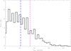 |
Fig. 1. Distribution of stars according to the number of peaks in their envelope. The dashed blue line indicates the mean number of peaks of the envelope and the purple dashed-dotted line indicates the value estimated by Lignières & Georgeot (2009). |
The observed asymmetry of the envelopes (see Fig. 2) is in agreement with the results in BF18. Around 62% of the envelopes have significantly higher asymmetry than the Sun (> 3σ), ∼45% towards lower frequency modes and ∼17% towards higher frequency modes. The higher number of cases towards lower frequencies may be indicative of the excitation mechanism for this kind of star.
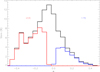 |
Fig. 2. Distribution of stars according to their asymmetry (black histogram). Blue (red) histogram denotes the proportion of stars whose νmax deviation from the mean frequency of the envelope towards lower (higher) frequencies is significantly higher than the solar case (see text). |
3.1. The  scaling relation
In order to calculate the parameters of this scaling relation we used several techniques. Following the steps in BF18 but including all the stars of the current sample, we made a linear fit between the measured temperatures Teff and νmax (LFIT, see Table 1 and Fig. 3). To test the probability that the relation between these two parameters is not random, we used the Pearson correlation (r) and the probability of being uncorrelated (Pu; i.e. Taylor 1997). This last parameter represents the probability that N measurements of a priori two uncorrelated variables give a specific Pearson correlation or higher (|r|≥r0). For example, in the present case, the probability of being uncorrelated with a Pearson correlation coefficient of R ∼ 0.55 is around
 (8)
(8)
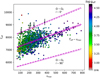 |
Fig. 3. Relation between νmax and |

Parameters of the  relation for each method.
where Γ(x) is the gamma function, and N is the number of δ Scuti stars of the sample. Therefore, we find a statistically significant correlation (Pu ≤ 1%). In addition, comparing our results with those of BF18, we noted that the higher number of stars of this kind we add, the lower the probability that these two parameters are uncorrelated although they have similar dispersion values (σ; see Table 1). As BF18 suggest in their study, this dispersion may be produced by the gravity-darkening effect since 99.3% of the sample lie inside the expected temperature regime.
For the second technique (MFIT), we calculated the mean effective temperature for each 10 μHz bin of the νmax. In that way, the different contributions of the departure of temperature ( ) produced by gravity-darkening are cancelled (see Sect. 1). This is only possible if there are a significant number of stars with a representative amount of different orientations. Then, we only took into account those bins with a population higher than 1% of the total number of stars (see Fig. 4). Once we had those values, we made the fit finding a linear relation with a Pearson coefficient of 0.972. The difference between the parameters obtained from the previous technique can be explained with the shorter range we are forced to take.
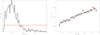 |
Fig. 4. Left panel: population of stars for each 10 μHz bin of νmax. The red solid line indicates the threshold we used to calculate the MFIT (see text). Right panel: scaling relation found using MFIT. |
The third method (KFIT) requires a knowledge of the structural parameters of the δ Scuti stars. We selected eight CoRoT δ Scuti stars from Sismo-channel whose temperature (Teff), rotation rate (Ω/ΩC), and inclination (i) had been obtained in other studies (see Table 2 in BF18). Using Eq. (4), we calculated their departure of temperature  and, finally, their mean effective temperature
  . Then, we made the
  linear fit. We find a similar relation to BF18 but with higher correlation. We note that the relative differences of mean temperature between all these methods are lower than 5% (see Sect. 4 for further discussion).
3.2. Mean effective gravity
To study the effect of the evolutionary stage on the frequency distribution, Bowman & Kurtz (2018) analysed the power spectra of a large sample of δ Scuti stars, including hybrids. They separated their sample taking into account the measured effective gravity, geff, considering three different groups: ZAMS (log geff ≳ 4.), MAMS (3.5 ≲ log geff ≲ 4.0), and TAMS (log geff ≲ 3.5), for zero-, mid-, and terminal-age main sequence stars, respectively. They conclude that each evolutionary stage should be treated separately.
Here, we perform the same excercise but taking into account the gravity-darkening effect. To calculate the mean effective gravity ( ), intrinsic to the star, we use von Zeipel’s law (von Zeipel 1924)
 (9)
(9)
where β ∼ 1 for stars with a fully radiative envelope (Claret 1998); and we obtain  with the LFIT scaling relation. Since we can recover
  for 1390 of our δ Scuti stars sample (see Fig. 5), it is possible to observe whether the evolutionary stage affects the
  relation. In order to study the dependence of the parameters of the scaling relation with
  , we divided our sample into several groups of
  bins.
bins.
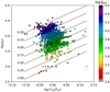 |
Fig. 5. Measured surface gravity vs. the ratio between measured and mean effective temperature. Different colours for each star indicate their mean surface gravity |


First of all, we observed that there is a top limit for νmax related to the mean surface gravity (νd). To exclude spurious candidates, we defined this parameter as the top frequency that contains the 99% of δ Scuti stars of its group (see left panels in Fig. 6). We find its dependence with the mean surface gravity with a linear fit,
 (10)
(10)
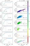 |
Fig. 6. From bottom to top, left panels: cumulative histogram of the population of stars per νmax and higher |


where the frequency is in μHz and the mean surface gravity in centimetre-gram-second.
Secondly, we made a  linear fit for each mean surface gravity group (see Fig. 6). We have not taken into account those groups with a low population or those stars with νmax > νd. Thus we only take into account those frequency bins with enough stars to cancel the contribution of the gravity-darkening effect (see Sect. 1). Once we had the scaling relation for each
  group (see Table 2), we observed that they change with the mean surface gravity. Then, we calculated the dependence of the slope and the y-intercept with this parameter,
 (11)
(11)
Parameters of the  relation for each
  group.
Once we obtained all parameters (ai), we used the improved  relation in Eq. (9) to recalculate the mean surface gravity, improving the selection of the respective group for each star. We repeated this process, iterating until the variation of the parameters was negligible (δai/ai < 10−4%). After a few iterations, we obtained the parameters of the improved
  scaling relation (see Table 3) with a probability of being uncorrelated of 8 × 10−212%.
Parameters of the improved  (
( relation.
Finally, we find a scaling relation between the frequency at maximum power and two intrinsic parameters of δ Scuti star structure. To calculate both  and
and  for an individual star, we iterate Eqs. (11) and (9) until these parameters converge to stable values. To test this method, we simulated ∼109 stars with known
  ,
,  , Ω/ΩC, and i. We added gaussian noise to their derived Teff, geff and νmax of the same order of magnitude as expected from the CoRoT, Kepler, and TESS catalogues. As we noted in Fig. 7, our method allows us to recover the exact value of the mean effective temperature with a precision error up to 4%. We also find a similar accuracy for the mean effective gravity with a deviation up to 2% and an error up to 8%.
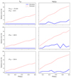 |
Fig. 7. Precision and accuracy of our methodology. The relative errors of the mean effective temperature (left) and mean effective surface gravity (right panels) have been calculated for typical photometric temperature errors (from top to bottom) and for different error values of surface gravity. |
4. Discussion
We noted that for equal  , the lowest
  δ Scuti stars excite the lowest frequencies (see bottom right panel of Fig. 6). Then, older stars should have lower frequency ranges as was predicted by Christensen-Dalsgaard et al. (2000). The highest frequency limit, ∼800 μHz, was already pointed out by Bowman & Kurtz (2018) although they only take into account the maximum amplitude peak, ν0, instead of νmax. To choose a proper parameter to calculate the mean effective temperature is of importance to constrain the rotation and inclination for each star (see Sect. 4.1). However, BF18 proved that there are no significant differences between the use of both parameters to calculate the scaling relation but ν0 produces a slightly higher dispersion and lower correlation due to the asymmetry of the envelope (see Sect. 4.2 for further discussion). We repeated the same test with our improved scaling relation (Eq. (11)) and found similar parameters within 1σ error (see Table 3). Therefore, combination frequencies should not significantly affect our results. In addition, there are several studies, both theoretical (e.g. Moskalik 1985; Nowakowski 2005) and observational (e.g. Breger & Montgomery 2014; Barceló Forteza et al. 2015; Saio et al. 2018) suggesting that peaks nearly or equal to combination of other frequencies may be resonantly-excited modes. Therefore, these modes should be taken into account to calculate νmax.
Another phenomenon we observe is a higher dispersion of temperatures for lower  groups (σ, see Table 1 and Fig. 6). The gravity-darkening effect depends on the ratio between centrifugal and gravity forces, ϵ2 (see Eq. (4)). Rewriting Eq. (5) as
 (12)
(12)
we noted that a higher rotation is required for more dense stars to have the same ϵ2, that is, the same departure of temperature. Combining the gravity-darkening effect and stellar evolution theory, we may explain the behaviour of temperature dispersion since radius increases with age (Christensen-Dalsgaard et al. 2000). Assuming that the observed dispersion (σ) is produced by the gravity-darkening effect, we can define the threshold rotation rate (ΩT) as the minimum rotation needed to observe a departure of temperature equal to σ. We can calculate the minimum rotation rate of a particular departure of temperature assuming a pole-on or equator-on star since intermediate values of inclination require higher values of rotation (see Sect. 1 and BF18). We use a numerical technique to calculate this parameter (see Sect. 4.1 for further details). Our results suggest that ΩT/ΩC decrease with the mean surface gravity (see Fig. 8) with the form
 (13)
(13)
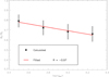 |
Fig. 8. Threshold rotation rate per mean surface gravity for δ Scuti stars. Black asterisks are the calculated values for each group (see text). The red line is a linear fit. |
and, therefore, increase with age. This effect does not mean that rotation should increase with age (contrary to gyrochronology predictions; e.g. Soderblom 2010), but it might decrease less than density. In any case, all the values of ΩT/ΩC are in agreement with the large number of fast rotators for A-type stars found by Royer et al. (2007): Ω ≳ 0.5ΩC.
4.1. i – Ω maps
Barceló Forteza et al. (2018) calculated the minimum rotation rate (Ωmin) for ∼700 pure δ Scuti stars. This parameter can be obtained using Eq. (4) and assuming the star is pole-on or equator-on. Furthermore, the limits of the inclination from the line of sight (i) can also been obtained assuming Ω ∼ ΩC. However, the observed departure of temperature should be higher than the relative error of the measurement
 (14)
(14)
to avoid the i − Ω degeneracy zone (see Figs. 5 and 6 in BF18). This zone does not allow us to use this technique to differentiate between a moderate or slow rotator with any inclination from a extreme rotator with an inclination close to the mid-latitude (i ∼ 55°). In that case a more detailed study is needed (e.g. Poretti et al. 2009; García Hernández et al. 2013; Escorza et al. 2016; Barceló Forteza et al. 2017).
We used a different technique to obtain a map with all possible combinations of i − Ω. This method simulates around one million stars with different i − Ω values and only selects those that fulfil the observed departure of temperature  (see Fig. 9).
 |
Fig. 9. Inclination – rotation (i − Ω) map of the Keplerδ Scuti star KIC 11823661. Red points are the models with the exact value of observed departure of temperature. Black points represent those models that take into account the error bars. |
To calculate the correct  , we take into account the improved scaling relation (Eq. (11)). However, this it is not always possible since we may not know the measured geff. In that case we use the LFIT scaling relation. The limits of rotation and inclination for the stars of our sample (see Table A.1), including i − Ω maps, are only available at the CDS.
We find only five δ Scuti stars are out of the expected temperature range for fast rotators: δTeff, obs ≲ −21.5% or δTeff, obs ≳ 14.5%. The surface gravity of the other 4 outsiders is unknown. These stars may be (pre-)extremely low mass stars since they have similar frequency ranges and similar or higher surface gravity (Sánchez Arias et al. 2018).
4.2. Mode variations with time
There are several reasons to use νmax instead of ν0 apart from its lower correlation. First of all, the visibility of the highest amplitude mode depends on the point of view of the observer (see Lignières & Georgeot 2009). Second, the highest amplitude mode is not fixed, meaning the amplitudes can change with time and other modes can become the highest amplitude mode (i.e. Handler et al. 1998; Breger 2000b; Barceló Forteza et al. 2015). This is not the case for νmax, which remains approximately constant during the cyclic changes (see Fig. 10). To study the variability of ν0 and νmax with time for stars with detected cyclic variations, we used the δSBF pipeline for each 20-d segment and we compared the results with those of the entire light curve. To find a sample of stars with cyclic variations, we studied the power spectrum of the entire light curve for all pure δ Scuti stars of our sample. There, the variations in the parameters of a mode are observed as split peaks of this mode (e.g. Moskalik 1985; Shibahashi & Kurtz 2012, see also Fig. 11), that is, as a multiplet. The frequency shift between peaks, the ratio of amplitudes, and the symmetry of the multiplet may indicate the nature of the variation. On one hand, a symmetric multiplet could indicate a superNyquist frequency mode (Murphy et al. 2013) or a binarity nature of the system (e.g. Shibahashi & Kurtz 2012; Murphy et al. 2014). On the other hand, an asymmetric multiplet could indicate a cyclic variation such as resonant mode coupling (RMC; Moskalik 1985; Barceló Forteza et al. 2015) or, in extreme cases, may suggest a definitive change in the stellar structure (Bowman & Kurtz 2014). Figure 10 shows the variation of ν0 and νmax for five pure δ Scuti stars with detected variations in some of their peaks in agreement with RMC. The sharp changes of ν0 with time can be compared with νmax 20-d measurements. In fact, the ν0 mean of the 20-d light curves is not in agreement with the value obtained with the entire light curve in all tested cases. This is not the case for νmax since both values are equal within errors. Resonances seem not to modify νmax at least in the long term.
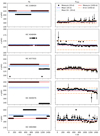 |
Fig. 10. Frequency of the highest amplitude peak (ν0, left panels) and frequency at maximum power (νmax, right panels) with time for five pure δ Scuti stars with detected resonant mode coupling (one per row; see text). Black circles represent the measurements of each parameter for 20-day segments of the entire light curve. The blue dashed line is the mean value of all 20-d measurements and cyan dotted lines are their error. The red line is the measurement of each parameter for a 1450-day light curve and the orange dashed-dotted lines are their error. The error bars for 20-d measurements of ν0 are smaller than the symbol. For clarity reasons, we only plotted the error bars for 20-d measurements of νmax for those outside of the 1450-d measure error. |
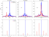 |
Fig. 11. Multiplets with one (left), symmetric (middle), and asymmetric (right panels) sidelobes. Top panels: detail of the original ten-point oversampled power spectrum (blue) and also after extracting the central peak (red). Bottom panels: detected peaks using δSBF taking into account the frequency shift between split peaks and their amplitude ratios. Blue points to the central peak and red points to split peaks. |
In this study, we also find that only 27% of pure δ Scuti stars have constant amplitude peaks (see Fig. 12). We recover the same proportion of stars with constant modes obtained by Bowman et al. (2016) if we take into account hybrid stars (38%). We observe that the other 73% of pure δ Scuti stars have modes with detected amplitude and/or phase variations. Looking at these phenomena for each  group, we observe significant differences. The lower the surface gravity, the larger the fraction of δ Scuti stars with detected variable modes (from 52% to 76%), especially for those with asymmetric multiplets (from 16% to 35%), including those candidates to have RMC (from 5% to 20%). Moreover, these candidates with extrinsic causes of variation (superNyquist frequencies or binarity) are approximately constant with surface gravity (∼16%). Finally, the proportion of stars observed with multiplets of only one detected sidelobe is approximately constant too (∼27%). We also added this analysis star by star in Table A.1.
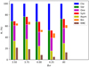 |
Fig. 12. Proportion of pure δ Scuti stars with constant (Cte) or variable (Var) modes for all the sample and for different evolutionary stages. This last kind can be differentiated by the shape of the multiplet: one sidelobe (One), symmetric (Sym) or asymmetric (Asym) sidelobes. (Bin) indicates the proportion of binary stars detected with this method (see text). RMC indicates the proportion of this kind of star that show multiplets affected by resonant mode coupling (see text). |
Our results suggest that the evolutionary stage seems to favour resonances towards older ages. This is in agreement with the increase of the g-mode frequencies with age (Christensen-Dalsgaard et al. 2000) and its interaction with p-modes. In addition, the transition stages may be observed as permanent changes in the power spectra of the stars due to their restructuring.
5. Advantages of 
Once we have the parameters of the scaling relation, we can use Eq. (11) to obtain the mean effective temperature of other pure δ Scuti stars. We analysed the power spectra of 239 δ Scuti candidates observed by CoRoT Exo-channel (Debosscher et al. 2009), calculating the  for 174 of them (see Table A.2 only at the CDS). The Teff of these stars were estimated by fitting their spectral energy distribution to a grid of theoretical models (Kurucz, Castelli et al. 1997) using the Virtual Observatory tool (VOSA, Bayo et al. 2008). Extinction was left as a free parameter in the spectral energy distribution fitting process, ranging from zero to the value obtained from the NASA/IPAC Galactic Dust Reddening and Extinction service2 using (Schlafly & Finkbeiner 2011)
Figure 13 compares the effective temperatures obtained with VOSA (red bars) with those available in the COROTSKY Database (blue bars; Charpinet et al. 2006). We can see how the assumption of no extinction for the majority of the objects in COROTSKY leads to an underestimation of the temperatures. This effect may cause a misclassification since cool δ Scuti stars are discarded and other kinds of hot pulsators are included.
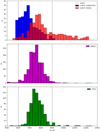 |
Fig. 13. Top panel: histogram of temperatures for 239 δ Scuti star candidates observed by CoRoT. Blue bars point to values from COROTSKY database (Charpinet et al. 2006) and red bars point to the values obtained with VOSA (see text). Dotted lines represent the temperature limits for δ Scuti stars (Uytterhoeven et al. 2011). Middle and bottom panels: same as top panel for stars of our main sample observed by Kepler and TESS, respectively. |
Moreover, different models based on different physical properties, may produce results with discrepancies up to the same order of magnitude (Sarro et al. 2013). For example, rotation can modify the observed colours (Collins & Smith 1985) with the consequent impact on temperature. In contrast,  seem not to depend on these parameters. Therefore, we can conclude that the scaling relation based on νmax allows us to characterize δ Scuti stars independently of rotation and also independently of extrinsic parameters of the star such as extinction.
6. Conclusions
The relation between the power-spectral structure and the structural parameters for δ Scuti stars has been a long-standing debate, especially since the beginning of large surveys using space telescopes (e.g. Balona & Dziembowski 2011; Moya et al. 2017). In this work, we have studied the oscillation spectra of 2372 A-F pulsating stars observed by CoRoT, Kepler, and TESS. Of these, 1442 were pure δ Scuti stars. Once their power spectra had been characterized, we obtained the empirical scaling relation between the frequency at maximum power, the mean effective temperature, and the mean surface gravity (Eq. (11)). This is in agreement with the predicted frequency distribution for the κ-mechanism (Dziembowski 1977) since we detected higher frequency modes for higher temperature δ Scuti stars. In fact, our relation is similar to that found by Barceló Forteza et al. (2018). We also observed that old stars with low surface gravity present lower frequency ranges (see Eq. (10) and Fig. 6), the opposite to young δ Scuti stars. This is also in agreement with predictions (Christensen-Dalsgaard et al. 2000). Therefore, the evolutionary stage affects the  relation and it must be taken into account to find the intrinsic parameters of this kind of star (
 ).
).
Photometric and spectroscopic techniques to measure the temperature (Teff) and the surface gravity (geff) may be significantly affected by the gravity-darkening effect (von Zeipel 1924). We have developed a methodology to correct such an effect by iterating Eqs. (9) and (11) until convergence. Gravity darkening may also explain the observed dispersion of the scaling relation (σ) and its decrease with  (see Table 2). Our results suggest that ageing stars may decrease their rotation more slowly than their density, making them closer to their break-up frequency. Thanks to the departure of temperature of each individual star (Eq. (4)), we have delimited rotation and inclination from the line of sight, especially for fast rotators. Thus, it is possible to correct the position of the star in the HR Diagram and then improve the age determination using isochrone fitting (e.g. Michel et al. 1999; Fox Machado et al. 2006). In addition, since δ Scuti stars are used as standard candles (e.g. McNamara 2011; Ziaali et al. 2019), it would be feasible to improve the distance determination to globular clusters and other galaxies. Moreover, exoplanetary research may benefit from our method since the calculation of the habitable zone depends on stellar parameters such as
  (Kopparapu et al. 2014).
In conclusion, we suggest the use of frequency at maximum power (νmax; see Eq. (1)) as a seismic index since it is a proper indicator of the mean temperature and surface gravity of the star. It is independent of rotation and extrinsic parameters such as inclination or extinction. Furthermore, νmax is not as affected by resonances as the highest amplitude mode (ν0). This property is especially useful for older stars since age benefits the interaction between modes (see Fig. 12). Finally, νmax variation may indicate the restructuring of the stars and their power spectra between different transition stages.
Mikulski Archive for Space Telescopes:
Acknowledgments
Comments from J. A. Caballero are gratefully acknowledged. The authors wish to thank the referee for useful suggestions that improved the paper. We also thank the CoRoT, Kepler, and TESS teams whose efforts made these results possible. The CoRoT space mission was developed and operated by CNES, with contributions from Austria, Belgium, Brazil, ESA (RSSD and Science Program), Germany and Spain. Funding for Kepler’s Discovery mission is provided by NASA’s Science Mission Directorate. Funding for the TESS mission is provided by the NASA Explorer Program. The authors acknowledge the effort made by TASOC WG4 that helped us in our target selection. This publication makes use of VOSA, developed under the Spanish Virtual Observatory project supported by the Spanish MICIU through Grant AyA2017-84089. VOSA has been partially updated by using funding from the European Union’s Horizon 2020 Research and Innovation Programme, under Grant Agreement No. 776403 (EXOPLANETS-A). SBF and DB received financial support from the Spanish State Research Agency (AEI) Projects No. ESP2017-87676-C5-1-R and No. MDM-2017-0737 Unidad de Excelencia “María de Maeztu”- Centro de Astrobiología (INTA-CSIC). AM acknowledges funding from the European Union’s Horizon 2020 research and innovation program under the Marie Sklodowska-Curie Grant agreement No. 749962 (project THOT). SMR acknowledges financial support from the State Agency for Research of the Spanish MICIU through the “Center of Excellence Severo Ochoa” award to the Instituto de Astrofísica de Andalucía (SEV-2017-0709). JCS and AGH acknowledge funding support from Spanish public funds (including FEDER fonds) for research under project ESP2017-87676-C5-2-R and ESP2017-87676-C5-5-R. JCS also acknowledges support from project RYC-2012-09913 under the “Ramón y Cajal” program of the Spanish Ministry of Science and Education. AGH acknowledges support from “Universidad de Granada” under project E-FQM-041-UGR18 from “Programa Operativo FEDER 2014-2020” programme by "Junta de Andalucía" regional Government.
References
- Aerts, C. 2019, ArXiv e-prints [arXiv:1912.12300] [Google Scholar]
- Aerts, C., Christensen-Dalsgaard, J., & Kurtz, D. W. 2010, Asteroseismology (Springer Science+Business Media B.V.) [Google Scholar]
- Antoci, V., Cunha, M., Houdek, G., et al. 2014, ApJ, 796, 118 [NASA ADS] [CrossRef] [Google Scholar]
- Antoci, V., Cunha, M. S., Bowman, D. M., et al. 2019, MNRAS, 490, 4040 [NASA ADS] [CrossRef] [Google Scholar]
- Baglin, A., Auvergne, M., Barge, P., et al. 2006, ESA SP, 1306, 33 [Google Scholar]
- Balona, L. A., & Dziembowski, W. A. 2011, MNRAS, 417, 591 [NASA ADS] [CrossRef] [Google Scholar]
- Barceló Forteza, S., Michel, E., Roca Cortés, T., & García, R. A. 2015, A&A, 579, A133 [NASA ADS] [CrossRef] [EDP Sciences] [Google Scholar]
- Barceló Forteza, S., Roca Cortés, T., García Hernández, A., & García, R. A. 2017, A&A, 601, A57 [NASA ADS] [CrossRef] [EDP Sciences] [Google Scholar]
- Barceló Forteza, S., Roca Cortés, T., & García, R. A. 2018, A&A, 614, A46 [NASA ADS] [CrossRef] [EDP Sciences] [Google Scholar]
- Bayo, A., Rodrigo, C., Barrado Y Navascués, D., et al. 2008, A&A, 492, 277 [NASA ADS] [CrossRef] [EDP Sciences] [Google Scholar]
- Borucki, W. J., Koch, D., Basri, G., et al. 2010, Science, 327, 977 [NASA ADS] [CrossRef] [PubMed] [Google Scholar]
- Bowman, D. M., & Kurtz, D. W. 2014, MNRAS, 444, 1909 [NASA ADS] [CrossRef] [Google Scholar]
- Bowman, D. M., & Kurtz, D. W. 2018, MNRAS, 476, 3169 [NASA ADS] [CrossRef] [Google Scholar]
- Bowman, D. M., Kurtz, D. W., Breger, M., Murphy, S. J., & Holdsworth, D. L. 2016, MNRAS, 460, 1970 [NASA ADS] [CrossRef] [Google Scholar]
- Breger, M. 2000a, ASP Conf. Ser., 210, 3 [NASA ADS] [Google Scholar]
- Breger, M. 2000b, MNRAS, 313, 129 [CrossRef] [Google Scholar]
- Breger, M., & Montgomery, M. H. 2014, ApJ, 783, 89 [NASA ADS] [CrossRef] [Google Scholar]
- Brown, T. M., Latham, D. W., Everett, M. E., & Esquerdo, G. A. 2011, AJ, 142, 112 [NASA ADS] [CrossRef] [Google Scholar]
- Castelli, F., Gratton, R. G., & Kurucz, R. L. 1997, A&A, 318, 841 [NASA ADS] [Google Scholar]
- Catelan, M., & Smith, H. A. 2015, Pulsating Stars (Wiley-VCH) [CrossRef] [Google Scholar]
- Chaplin, W. J., & Miglio, A. 2013, ARA&A, 51, 353 [NASA ADS] [CrossRef] [Google Scholar]
- Charpinet, S., Cuvilo, J., Platzer, J., et al. 2006, ESA SP, 1306, 353 [NASA ADS] [Google Scholar]
- Chevalier, C. 1971, A&A, 14, 24 [NASA ADS] [Google Scholar]
- Christensen-Dalsgaard, J. 2000, ASP Conf. Ser., 210, 187 [NASA ADS] [Google Scholar]
- Claret, A. 1998, A&AS, 131, 395 [NASA ADS] [CrossRef] [EDP Sciences] [Google Scholar]
- Collins, G. W. I., & Smith, R. C. 1985, MNRAS, 213, 519 [NASA ADS] [CrossRef] [Google Scholar]
- Debosscher, J., Sarro, L. M., López, M., et al. 2009, A&A, 506, 519 [NASA ADS] [CrossRef] [EDP Sciences] [Google Scholar]
- de Franciscis, S., Pascual-Granado, J., Suárez, J. C., et al. 2019, MNRAS, 487, 4457 [Google Scholar]
- Dziembowski, W. 1977, Acta Astron., 27, 203 [NASA ADS] [Google Scholar]
- Dziembowski, W. 1997, IAU Symp., 181, 317 [NASA ADS] [Google Scholar]
- Escorza, A., Zwintz, K., Tkachenko, A., et al. 2016, A&A, 588, A71 [NASA ADS] [CrossRef] [EDP Sciences] [Google Scholar]
- Fox Machado, L., Pérez Hernández, F., Suárez, J. C., Michel, E., & Lebreton, Y. 2006, A&A, 446, 611 [NASA ADS] [CrossRef] [EDP Sciences] [Google Scholar]
- García, R. A., Mathur, S., Pires, S., et al. 2014, A&A, 568, A10 [NASA ADS] [CrossRef] [EDP Sciences] [Google Scholar]
- García Hernández, A., Moya, A., Michel, E., et al. 2013, A&A, 559, A63 [NASA ADS] [CrossRef] [EDP Sciences] [Google Scholar]
- García Hernández, A., Martín-Ruiz, S., Monteiro, M. J. P. F. G., et al. 2015, ApJ, 811, L29 [NASA ADS] [CrossRef] [Google Scholar]
- Handler, G., Pamyatnykh, A. A., Zima, W., et al. 1998, MNRAS, 295, 377 [NASA ADS] [CrossRef] [Google Scholar]
- Jeffery, C. S. 2008, Commun. Asteroseismol., 157, 240 [NASA ADS] [Google Scholar]
- Kjeldsen, H., & Bedding, T. R. 1995, A&A, 293, 87 [NASA ADS] [Google Scholar]
- Kopparapu, R. K., Ramirez, R. M., SchottelKotte, J., et al. 2014, ApJ, 787, L29 [NASA ADS] [CrossRef] [Google Scholar]
- Lignières, F., & Georgeot, B. 2009, A&A, 500, 1173 [NASA ADS] [CrossRef] [EDP Sciences] [Google Scholar]
- McNamara, D. H. 2011, AJ, 142, 110 [NASA ADS] [CrossRef] [Google Scholar]
- Michel, E., Dupret, M. A., Reese, D., et al. 2017, Eur. Phys. J. Web Conf., 160, 03001 [Google Scholar]
- Michel, E., Hernández, M. M., Houdek, G., et al. 1999, A&A, 342, 153 [NASA ADS] [Google Scholar]
- Moskalik, P. 1985, Acta Astron., 35, 229 [NASA ADS] [Google Scholar]
- Moya, A., Suárez, J. C., García Hernández, A., & Mendoza, M. A. 2017, MNRAS, 471, 2491 [NASA ADS] [CrossRef] [Google Scholar]
- Moya, A., Barceló Forteza, S., Bonfanti, A., et al. 2018, A&A, 620, A203 [NASA ADS] [CrossRef] [EDP Sciences] [Google Scholar]
- Murphy, S. J., Shibahashi, H., & Kurtz, D. W. 2013, MNRAS, 430, 2986 [NASA ADS] [CrossRef] [Google Scholar]
- Murphy, S. J., Bedding, T. R., Shibahashi, H., Kurtz, D. W., & Kjeldsen, H. 2014, MNRAS, 441, 2515 [Google Scholar]
- Nowakowski, R. M. 2005, Acta Astron., 55, 1 [NASA ADS] [Google Scholar]
- Pérez Hernández, F., Claret, A., Hernández, M. M., & Michel, E. 1999, A&A, 346, 586 [NASA ADS] [Google Scholar]
- Poretti, E., Michel, E., Garrido, R., et al. 2009, A&A, 506, 85 [NASA ADS] [CrossRef] [EDP Sciences] [Google Scholar]
- Royer, F., Zorec, J., & Gómez, A. E. 2007, A&A, 463, 671 [NASA ADS] [CrossRef] [EDP Sciences] [Google Scholar]
- Saio, H., Bedding, T. R., Kurtz, D. W., et al. 2018, MNRAS, 477, 2183 [Google Scholar]
- Sánchez Arias, J. P., Romero, A. D., Córsico, A. H., et al. 2018, A&A, 616, A80 [NASA ADS] [CrossRef] [EDP Sciences] [Google Scholar]
- Sarro, L. M., Debosscher, J., Neiner, C., et al. 2013, A&A, 550, A120 [NASA ADS] [CrossRef] [EDP Sciences] [Google Scholar]
- Schlafly, E. F., & Finkbeiner, D. P. 2011, ApJ, 737, 103 [NASA ADS] [CrossRef] [Google Scholar]
- Shibahashi, H., & Kurtz, D. W. 2012, MNRAS, 422, 738 [NASA ADS] [CrossRef] [Google Scholar]
- Soderblom, D. R. 2010, ARA&A, 48, 581 [NASA ADS] [CrossRef] [Google Scholar]
- Stassun, K. G., Oelkers, R. J., Paegert, M., et al. 2019, AJ, 158, 138 [Google Scholar]
- Suárez, J. C., García Hernández, A., Moya, A., et al. 2014, A&A, 563, A7 [NASA ADS] [CrossRef] [EDP Sciences] [Google Scholar]
- Taylor, J. 1997, Introduction to Error Analysis, the Study of Uncertainties in Physical Measurements, 2nd Edition. (University Science Books) [Google Scholar]
- Uytterhoeven, K., Moya, A., Grigahcène, A., et al. 2011, A&A, 534, A125 [NASA ADS] [CrossRef] [EDP Sciences] [Google Scholar]
- von Zeipel, H. 1924, MNRAS, 84, 684 [NASA ADS] [CrossRef] [Google Scholar]
- Xiong, D. R., Deng, L., Zhang, C., & Wang, K. 2016, MNRAS, 457, 3163 [NASA ADS] [CrossRef] [Google Scholar]
- Ziaali, E., Bedding, T. R., Murphy, S. J., Van Reeth, T., & Hey, D. R. 2019, MNRAS, 486, 4348 [NASA ADS] [CrossRef] [Google Scholar]
All Tables
All Figures
|
Fig. 1. Distribution of stars according to the number of peaks in their envelope. The dashed blue line indicates the mean number of peaks of the envelope and the purple dashed-dotted line indicates the value estimated by Lignières & Georgeot (2009). |
| In the text | |
|
Fig. 2. Distribution of stars according to their asymmetry (black histogram). Blue (red) histogram denotes the proportion of stars whose νmax deviation from the mean frequency of the envelope towards lower (higher) frequencies is significantly higher than the solar case (see text). |
| In the text | |
|
Fig. 3. Relation between νmax and |
| In the text | |
|
Fig. 4. Left panel: population of stars for each 10 μHz bin of νmax. The red solid line indicates the threshold we used to calculate the MFIT (see text). Right panel: scaling relation found using MFIT. |
| In the text | |
|
Fig. 5. Measured surface gravity vs. the ratio between measured and mean effective temperature. Different colours for each star indicate their mean surface gravity |
| In the text | |
|
Fig. 6. From bottom to top, left panels: cumulative histogram of the population of stars per νmax and higher |
| In the text | |
|
Fig. 7. Precision and accuracy of our methodology. The relative errors of the mean effective temperature (left) and mean effective surface gravity (right panels) have been calculated for typical photometric temperature errors (from top to bottom) and for different error values of surface gravity. |
| In the text | |
|
Fig. 8. Threshold rotation rate per mean surface gravity for δ Scuti stars. Black asterisks are the calculated values for each group (see text). The red line is a linear fit. |
| In the text | |
|
Fig. 9. Inclination – rotation (i − Ω) map of the Keplerδ Scuti star KIC 11823661. Red points are the models with the exact value of observed departure of temperature. Black points represent those models that take into account the error bars. |
| In the text | |
|
Fig. 10. Frequency of the highest amplitude peak (ν0, left panels) and frequency at maximum power (νmax, right panels) with time for five pure δ Scuti stars with detected resonant mode coupling (one per row; see text). Black circles represent the measurements of each parameter for 20-day segments of the entire light curve. The blue dashed line is the mean value of all 20-d measurements and cyan dotted lines are their error. The red line is the measurement of each parameter for a 1450-day light curve and the orange dashed-dotted lines are their error. The error bars for 20-d measurements of ν0 are smaller than the symbol. For clarity reasons, we only plotted the error bars for 20-d measurements of νmax for those outside of the 1450-d measure error. |
| In the text | |
|
Fig. 11. Multiplets with one (left), symmetric (middle), and asymmetric (right panels) sidelobes. Top panels: detail of the original ten-point oversampled power spectrum (blue) and also after extracting the central peak (red). Bottom panels: detected peaks using δSBF taking into account the frequency shift between split peaks and their amplitude ratios. Blue points to the central peak and red points to split peaks. |
| In the text | |
|
Fig. 12. Proportion of pure δ Scuti stars with constant (Cte) or variable (Var) modes for all the sample and for different evolutionary stages. This last kind can be differentiated by the shape of the multiplet: one sidelobe (One), symmetric (Sym) or asymmetric (Asym) sidelobes. (Bin) indicates the proportion of binary stars detected with this method (see text). RMC indicates the proportion of this kind of star that show multiplets affected by resonant mode coupling (see text). |
| In the text | |
|
Fig. 13. Top panel: histogram of temperatures for 239 δ Scuti star candidates observed by CoRoT. Blue bars point to values from COROTSKY database (Charpinet et al. 2006) and red bars point to the values obtained with VOSA (see text). Dotted lines represent the temperature limits for δ Scuti stars (Uytterhoeven et al. 2011). Middle and bottom panels: same as top panel for stars of our main sample observed by Kepler and TESS, respectively. |
| In the text | |
Current usage metrics show cumulative count of Article Views (full-text article views including HTML views, PDF and ePub downloads, according to the available data) and Abstracts Views on Vision4Press platform.
Data correspond to usage on the plateform after 2015. The current usage metrics is available 48-96 hours after online publication and is updated daily on week days.
Initial download of the metrics may take a while.