| Issue |
A&A
Volume 637, May 2020
|
|
|---|---|---|
| Article Number | A91 | |
| Number of page(s) | 36 | |
| Section | Astrophysical processes | |
| DOI | https://doi.org/10.1051/0004-6361/202037492 | |
| Published online | 27 May 2020 | |
Wind morphology around cool evolved stars in binaries
The case of slowly accelerating oxygen-rich outflows⋆
1
Center for mathematical Plasma Astrophysics, Department of Mathematics, KU Leuven, Celestijnenlaan 200B, 3001 Leuven, Belgium
e-mail: This email address is being protected from spambots. You need JavaScript enabled to view it.
2
Institute of Astronomy, KU Leuven, Celestijnenlaan 200D B2401, 3001 Leuven, Belgium
Received:
13
January
2020
Accepted:
30
March
2020
Abstract
Context. The late evolutionary phase of low- and intermediate-mass stars is strongly constrained by their mass-loss rate, which is orders of magnitude higher than during the main sequence. The wind surrounding these cool expanded stars frequently shows nonspherical symmetry, which is thought to be due to an unseen companion orbiting the donor star. The imprints left in the outflow carry information about the companion and also the launching mechanism of these dust-driven winds.
Aims. We study the morphology of the circumbinary envelope and identify the conditions of formation of a wind-captured disk around the companion. Long-term orbital changes induced by mass loss and mass transfer to the secondary are also investigated. We pay particular attention to oxygen-rich, that is slowly accelerating, outflows in order to look for systematic differences between the dynamics of the wind around carbon and oxygen-rich asymptotic giant branch (AGB) stars.
Methods. We present a model based on a parametrized wind acceleration and a reduced number of dimensionless parameters to connect the wind morphology to the properties of the underlying binary system. Thanks to the high performance code MPI-AMRVAC, we ran an extensive set of 72 three-dimensional hydrodynamics simulations of a progressively accelerating wind propagating in the Roche potential of a mass-losing evolved star in orbit with a main sequence companion. The highly adaptive mesh refinement that we used, enabled us to resolve the flow structure both in the immediate vicinity of the secondary, where bow shocks, outflows, and wind-captured disks form, and up to 40 orbital separations, where spiral arms, arcs, and equatorial density enhancements develop.
Results. When the companion is deeply engulfed in the wind, the lower terminal wind speeds and more progressive wind acceleration around oxygen-rich AGB stars make them more prone than carbon-rich AGB stars to display more disturbed outflows, a disk-like structure around the companion, and a wind concentrated in the orbital plane. In these configurations, a large fraction of the wind is captured by the companion, which leads to a significant shrinking of the orbit over the mass-loss timescale, if the donor star is at least a few times more massive than its companion. In the other cases, an increase of the orbital separation is to be expected, though at a rate lower than the mass-loss rate of the donor star. Provided the companion has a mass of at least a tenth of the mass of the donor star, it can compress the wind in the orbital plane up to large distances.
Conclusions. The grid of models that we computed covers a wide scope of configurations: We vary the terminal wind speed relative to the orbital speed, the extension of the dust condensation region around the cool evolved star relative to the orbital separation, and the mass ratio, and we consider a carbon-rich and an oxygen-rich donor star. It provides a convenient frame of reference to interpret high-resolution maps of the outflows surrounding cool evolved stars.
Key words: accretion, accretion disks / stars: evolution / stars: winds, outflows / stars: AGB and post-AGB / methods: numerical / binaries: general
Movie associated to Fig. 7 is available at https://www.aanda.org
© ESO 2020
1. Introduction
As low- and intermediate-mass stars, which have initial masses ranging from 0.8 to 8 M⊙, evolve beyond the main sequence, they are bound to expand and cool down. Along the red giant branch (RGB), the effective gravity in the outermost layers drops and the mass-loss rate increases (Groenewegen 2012). During the subsequent asymptotic giant branch (AGB) phase, the mass-loss rate peaks at 10−7–10−5 M⊙ yr−1, with terminal wind speeds of 5–20 km s−1 (Knapp et al. 1998; Habing & Olofsson 2003; Herwig 2005; Ramstedt et al. 2009). By the time they eventually become white dwarfs, AGB stars have lost 35–85% of their mass (Marshall et al. 2004). The stars with an initial mass above ∼8 M⊙ undergo a phase where they manifest as red supergiants (RSG, Levesque 2010).
Through their winds, cool evolved stars represent a major source of dust and molecular enrichment for the interstellar medium (Groenewegen et al. 2002). Although the wind launching mechanism remains largely unknown for RSGs, a dust-driven model has been proved to be successful for AGB stars (see Höfner & Olofsson 2018, for a recent and comprehensive review). The κ-mechanism excites radial pulsations, which shoot out material and provoke the formation of internal shocks within a couple of stellar radii. The temperature of compressed gas decreases downstream of the shocks until it reaches temperatures of 1500 to 1800 K, which are low enough to trigger the condensation of gaseous species into dust grains, which absorb the stellar radiation, accelerate, and drag the ambient gas (Liljegren et al. 2016; Freytag et al. 2017). During their post-main sequence evolution, low- and intermediate-mass stars experience several dredge-up events, which bring freshly formed carbon to the outer envelope and can turn originally oxygen-rich (O-rich) stars into carbon-rich (C-rich) stars (Straniero et al. 1997; Herwig & Austin 2004) with dramatic consequences on the dust chemical content. Since the latter sets the dust opacity, the wind acceleration profile strongly differs around O-rich and C-rich AGB stars: The low opacity of dust grains that formed from O-rich gaseous environments leads to a much more progressive wind acceleration around O-rich AGB stars, where the wind reaches its terminal speed several tens of stellar radii away from the donor star (Decin et al. 2010a, 2018). A full understanding of dust-driven winds emitted by cool evolved stars requires a radiative hydro-chemical model of dust grain growth in an environment generally out of thermodynamic equilibrium (Boulangier et al. 2019a).
High spatial and spectral resolution instruments have shed unprecedented light on the complexity of the astrochemistry at work in these cool winds. While the Hubble Space Telescope ushered in a new era of high-resolution imaging in the optical wavelength range, the infrared space telescope Spitzer revealed how diverse the wind properties can be around cool evolved stars in the Galaxy and also in the nearby Small and Large Magellanic Clouds (Dell’Agli et al. 2015; Yang et al. 2018). The Hubble Space Telescope captures the light scattered by the dust present in large quantities in the inner regions of the wind, but molecular line emission also contains invaluable information. The powerful spectrometers aboard Herschel and the (sub)millimeter interferometer ALMA granted us access to a plethora of rotational and vibrational lines originating up to several thousands of astronomical units (au) away from the cool evolved star. Thanks to multichannel molecular emission maps, the kinematic structure of the circumstellar flow can be characterized, thus opening the door to a full 3D reconstruction of the wind (Decin et al. 2018).
Significant nonspherical features in the wind of cool evolved stars have been identified thanks to these instruments; this has also been the case in the shape of planetary nebulae, which are thought to be the descendants of RGB and AGB stars (Shklovsky 1956). Recurrent axisymmetric patterns appear around cool evolved stars, such as compressed structures (disks or tori, Bujarrabal et al. 2016; Kamath et al. 2016), polar cavities, and spirals (Homan et al. 2018), in addition to arcs (Decin et al., in prep.). Although alternative explanations have been proposed (Nordhaus & Blackman 2006; Chita et al. 2008), the community has been progressively more inclined to attribute these features to the presence of an unseen companion. The reason for this shift in opinion stems from observations as well as new population synthesis results (Moe & Di Stefano 2017). In a few systems where nonspherical imprints are observed in the circumstellar environments, robust hints in favor of the presence of a companion have emerged. In these systems, it is still questioned, however, whether the companion is close enough to be responsible for producing these nonspherical features or if there is a third undetected object on a close orbit with the donor star. Around RGB stars with periodically modulated luminosities, simultaneous monitoring of the Doppler shift and of the light curve proved that these variations were due to the ellipsoidal deformation of the star due to the presence of a companion on a close orbit (sequence E long period variables, Nicholls et al. 2010). Furthermore, the complex morphology of the AGB wind in the Mira A B system has been shown to be partly due to a companion on approximately a 500-year orbit (Ramstedt et al. 2014).
The impact of binarity on stellar evolution cannot be overstated. Interactions in a close binary system modify the chemical stratification within the star and alter the evolution of its spin via mass and angular momentum exchanges with the orbiting companion (De Marco & Izzard 2017). It has been shown to be a key-ingredient in understanding Barium stars (Bidelman & Keenan 1951), SNe Ia as descendants of symbiotic binaries (Claeys et al. 2014), carbon and s-process enhanced metal-poor stars (Abate et al. 2013), and blue stragglers in old open clusters (Jofré et al. 2016). Classic Roche lobe overflow (RLOF) and wind accretion have been shown to be the two limit mass transfer mechanisms of generally more complex configurations. Numerical hydrodynamics simulations enabled hybrid regimes such as wind-RLOF to be identified (Mohamed & Podsiadlowski 2007), which turned out to be decisive in reconciling models and observations. They revealed enhanced mass transfer rates between the donor star, also called the primary, and the accretor, also called the secondary (Abate et al. 2013), and they confirmed the formation of wind-captured disks around the secondary (Huarte-Espinosa et al. 2013; de Val-Borro et al. 2017).
Grid-based and smooth particle hydrodynamics numerical simulations also reproduced large scale features left by the secondary in the wind of the donor star, such as arcs, spirals, and circumbinary disks, and they have evaluated the impact of the inclination of the orbit with the line-of-sight (Mastrodemos & Morris 1999; Liu et al. 2017; Chen et al. 2018; Saladino et al. 2019; Kim et al. 2019). However, the slow acceleration of O-rich outflows proved to be a challenging ingredient to account for, along with controlling the amount of kinetic energy per unit mass provided to the flow by the radiative pressure on dust grains. Resolving both the wind launching scale and the whole circumbinary outflow requires highly adaptive grids whose geometry matches the one of the outflow. As noted by Chen et al. (2017), spherical grids represent good candidates to move forward. This is why in this work, we developed a numerical framework based on a radially stretched spherical mesh centered on the donor star. It greatly facilitates the treatment of the wind launching, guarantees the conservation of angular momentum, and limits numerical artifacts introduced by the discretization of the equations (e.g., numerical diffusivity). It also enabled us to capture both the initial deviation of the wind by the secondary and the shaping of the circumbinary envelope up to several tens of orbital separations at a computational cost so low that we could cover a wide range of realistic sets of parameters. With the dimensionless parametrization we introduce, we can parametrically explore how the properties of the dust-driven acceleration and of the accreting companion determines the morphology of the outflow.
In Sect. 2, we present a model based on an empirical wind acceleration so as to reproduce a predefined velocity profile. We also identify the dimensionless parameters which determine the shape of the hydrodynamics solutions we solve in our numerical setup. In Sect. 3, we report on the main results of our comprehensive exploration of 70 configurations, which are representative of C-rich and O-rich AGB stars with an orbiting companion. It provides a grid of models spanning all of the possible configurations whose main properties are summarized and discussed in Sect. 4.
2. Model
2.1. Parametrized β-wind
In this section, we describe how the wind is accelerated from the donor star. The wind launching does not depend on time, and stellar pulsations are not included in the present model (see Chen et al. 2017, for a model with periodic modulations of the mass-loss rate through the radial outflow velocity). We used the classic β-wind velocity profile as a parametrization to compute the corresponding radiative acceleration term for an isolated star. This method guarantees that we control both the terminal speed and how quickly the wind reaches it, contrary to previously used approaches which parametrize the acceleration term directly: Alternatives include winds undergoing reverted gravity (Kim et al. 2019) or the free-wind model where radiation counterbalances the gravity exactly, leading to a constant wind speed (Liu et al. 2017) or a thermally-driven wind when thermal pressure is included (Saladino et al. 2019). An enforced β velocity profile alleviates the full radiative-hydrochemical computation required to determine the acceleration profile, allowing us to explore the impact of a wide range of realistic acceleration profiles at an affordable computational cost.
2.1.1. Pressureless test case
We first validated our approach in the simplest context: a pressureless purely radial wind in spherical geometry undergoing gravity and an outward radiative force whose large amplitude justified us neglecting the pressure force which drives thermal winds (Lamers & Cassinelli 1999). These radiatively-driven winds can be fit by a velocity profile called the β-law:
 (1)
(1)
where R0 is the distance to the stellar center where acceleration is triggered, v∞ is the terminal wind speed, and β is a positive exponent whose value determines how quickly the wind reaches its terminal speed, with a more progressive acceleration for a larger value of β. Around AGB stars, wind launching is believed to be made possible thanks to pulsations which lift material up to a distance, the dust condensation region, where the temperature is low enough and the density is high enough, due to shocks, for dust to form. Dust is a key-ingredient in the launching of these dust-driven winds. Indeed, thanks to the opacity of dust-grains in the optical and infra-red, the dust is provided with momentum by the stellar continuum thanks to radiative pressure. Once accelerating dust-grains redistribute their momentum to the ambient gas through Coulomb drag, a wind is launched (Höfner & Olofsson 2018). Due to the requirement for dust to be formed for this process to take place, the wind does not directly take off from the stellar photosphere, but rather at a radius called the dust condensation radius, Rd. Realistic dust opacity profiles lead to velocity profiles that are in excellent agreement with the β-law. Furthermore, the β-law matches the observations for C-rich and O-rich AGB stars (Decin et al. 2010b, 2015, 2018). Around other types of cool evolved stars, such as RSGs, the wind launching mechanism remains largely unknown, although the observed velocity profiles still reasonably match the aforementioned β-law (Decin et al. 2006).
For cool evolved stars, the terminal wind speed ranges between 5 and 20 km s−1 (Ramstedt et al. 2009). C-rich AGB stars lead to dust grains of high opacity, which strongly accelerate by the stellar radiative field. The terminal speed is reached within a few stellar radii, which yields a β exponent as low as 0.1 (Decin et al. 2015). Due to the low opacity of the dust grains that formed in their midst, winds surrounding O-rich AGB stars accelerate in a much more progressive way. Although observations can be fit with a high β exponent (∼5, Khouri et al. 2014), we currently lack theoretical justifications to reproduce velocity profiles analogous to β-laws with β = 5. If the wind is still radiation-driven, it would require a dramatic increase in the opacity of the dust-gas mixture that is far from the stellar photosphere.
The implementation of this configuration in a uni-dimensional numerical setup leads to the stable profile represented in Fig. 1 (blue solid line). The initial condition is a flat density profile with a zero-speed and the analytic solution is set at the inner boundary condition located at 1.01 R0. The acceleration source term is given by vβdvβ. This preliminary benchmark confirms the validity of the solving schemes used later on in the full 3D setup described in Sect. 2.3.
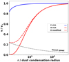 |
Fig. 1. Velocity profiles for a C-rich AGB star (solid blue line, β = 0.1) and for an O-rich AGB star (solid red line, β = 5), from 1.2 to 500 dust condensation radii. The red dashed line represents the modified β-law such that the wind is launched at a velocity slightly above the sound speed at the inner edge of the simulation space (β′ ∼ 6.7). The sound speed profile is the dotted black line and we assumed a fiducial terminal wind speed that is four times higher than the sound speed at the dust condensation radius. |
2.1.2. Modified β-wind
A specific difficulty for numerical simulations of winds around O-rich AGB stars arises from the low wind speed up to large distances. For C-rich AGB stars, the sonic point at the radius Rs is very close to the dust condensation radius, which ensures that the wind can be safely injected from r = Rd at the sound speed or slightly above, as it has been done in previous simulations (Kim et al. 2019). It prevents spurious reflections of acoustic waves at the injection border of the simulation box. For O-rich AGB stars though, such a procedure requires more caution since the wind might remain subsonic up to several stellar radii.
In case the β-law in Eq. (1) gives a subsonic wind speed at the inner edge of the simulation space, set at 1.2Rd, we needed to modify the β velocity profile such that the wind starts a few 0.01% above the local sound speed cs, s:
 (2)
(2)
where β′ was computed such that the terminal radius remains unchanged. This fix is generally needed for O-rich stars but not for C-rich stars. We computed the local sound speed assuming a radial temperature profile T ∝ r−0.6, which is in agreement with the observations, a temperature at the dust condensation radius of 1500 K, and a fiducial mean molecular weight of one proton mass. An additional argument in favor of the legitimacy of this approach comes from simulations of the flow structure in the innermost parts, between the stellar photosphere and the dust condensation radius. For instance, Freytag et al. (2017) performed simulations of the outer envelopes of AGB stars and found characteristic turbulent speeds associated with Mach numbers of two to three. In the current framework, the dynamics of the warm gas in-between the photosphere and the dust condensation radius is out of reach. Instead, we started our simulations at a radius 1.2 times larger than the dust condensation radius and prescribed launching conditions set by these velocity profiles, as described in more detail in Sect. 2.3. A modified β velocity profile is represented in Fig. 1 (red dashed line) where it can be seen that even for very slowly accelerating winds, the discrepancy with the classic β-law (red solid line) remains moderate. Hereafter, we write vβ for both the standard and modified β-law, depending on whether a correction is needed or not.
2.2. Binary system and equations
The aforementioned launching procedure guarantees that the right amount of kinetic energy per unit mass is progressively injected into the wind, given a certain predefined velocity profile. The modeling of the full binary can now be described. We worked in the frame corotating with the two bodies, at the orbital angular speed Ω, neglecting any eccentricity of the orbit. To limit the number of parameters, the star was assumed to have no spin since its significant radial expansion leads to a spin angular speed that is much lower than the orbital angular speed Ω. However, for a high mass of the secondary (i.e., q = 1), tidal coupling could significantly spin the donor star up to ∼20 au (Saladino et al. 2019). The strong dependency of the synchronization timescale on the ratio of the stellar radius to the orbital separation might also lead to fast spin-up in the donor star when it gets close to fill its Roche lobe (Zahn 1977; Keppens 1997; Keppens et al. 2000). We also discarded gas self-gravity and the feedback of the wind on the stellar masses and orbits, which were negligible over the course of our simulations.
The fundamental equations of hydrodynamics, which determine the evolution of the stellar wind, are the continuity equation and the conservation of linear momentum:
 (3)
(3)
 (4)
(4)
 (5)
(5)
where ρ, v, and P are the mass density, the velocity vector, and the pressure, respectively, while G is the gravitational constant. Additionally, 11 is the diagonal unity 3 by 3 matrix, ⊗ is the dyadic product, and ∧ is the cross product. The subscripts 1 and 2 refer to the donor star and to the secondary object, respectively, and Mi is the mass of body i and ri is the position vector with respect to body i. Finally, r is the position vector with respect to the center of mass of the two bodies. The first term on the right-hand side of Eq. (4) represents the gravitational influence of the secondary object and the second and third terms are the centrifugal and Coriolis forces. The last term includes the gravitational attraction of the donor star and the radiative acceleration, as described in Sect. 2.1, with vβ given by Eqs. (1) or (2). The orbital angular speed Ω is related to M1, M2, and the orbital separation a via Kepler’s third law. The coupling of the gas with the dust is encapsulated in this radiative acceleration term.
We need an additional equation to determine the evolution of the pressure entering Eq. (4). Ideally, this equation would account for the full thermodynamics of the problem and, in particular, for the heating by the stellar radiative field and re-emitting dust grains (Boulangier et al. 2019b,a) as well as for the electron and molecular cooling mechanisms. Instead, we rely on the following polytropic prescription to close the system of equations:
 (6)
(6)
where γ is the polytropic index and S is a constant, which can be related to the sound speed at the sonic point cs, s and the density at the sonic point ρs through  .
.
Physically, a polytropic index of 5/3 would mean that we neglect any net heating and cooling (adiabatic hypothesis), while a polytropic index of one would mean that heating and cooling are efficient enough to counterbalance any change of internal energy due to expansion or compression, respectively (isothermal hypothesis). To determine the suitable polytropic index to reproduce the observed temperature profile of T ∝ r−0.6, we follow this reasoning: due to the polytropic assumption and the ideal gas law, T ∝ ργ−1. In addition, due to mass conservation in spherical geometry, when the wind speed has reached the terminal speed, ρ ∝ r−2. Consequently, a polytropic index γ = 1.3 enables us to represent a realistic cooling and to match the observed temperature profile far from the star.
The wind is launched from a sphere of radius Rin = 1.2Rd with a density set by the sonic radius Rs with respect to Rin and a radial velocity given by the β-law, which can be modified if needed. The toroidal component of the velocity vector is set by the absence of spin of the donor star in the inertial frame of the observer.
We rely on the following length, speed and density normalization, which reduces the number of parameters that is needed to numerically compute the shape of the solutions to five: the condensation radius Rd, the orbital speed aΩ and the density at the sonic point ρs (linked to the mass-loss rate). The five fundamental dimensionless shape parameters which appear in the equations after normalization and entirely determine all possible numerical solutions are as follows:
– the mass ratio q = M1/M2,
– the dust condensation radius filling factor f = Rd/RR, 1, with RR, 1 the Roche lobe radius of the primary given by Eggleton (1983),
– the ratio of the terminal to the orbital speed η = v∞/(aΩ),
– the β exponent which sets the steepness of the velocity profile, and
– the ratio of the terminal speed to the sound speed at the dust condensation radius v∞/cs, d.
To identify the main dependencies of the wind morphology on these parameters, we considered different values for these parameters that are representative of AGB binaries. We used mass ratios of one and ten for an AGB star in orbit with a main sequence solar-type companion and with a low-mass star or a brown dwarf companion, respectively. The filling factor substantially varies from one system to another since both RGB and AGB donor stars can be large enough and/or the orbital separation can be small enough such that the dust condensation region (or even the star itself) might fill the Roche lobe. We worked with a filling factor of 5%, 20%, and 80% to study the impact of the stellar expansion and/or the secular evolution of the orbital parameters on the wind dynamics. To distinguish between the quickly accelerated winds of C-rich AGB stars and the slowly accelerating winds of O-rich AGB stars, we considered two β exponents. For a C-rich AGB star, the wind quickly accelerates and β = 0.1 is consistent with observations and theoretically founded. For winds from O-rich AGB stars, the theoretical framework is incomplete and the choice of β can only be motivated by observational insights. Given how slowly accelerating O-rich winds accelerate, we use the fiducial value β = 5 (see Sect. 2.1.1). The launching of O-rich winds requires a sustained line-acceleration up to large distances; this is a mechanism we discuss in more detail in Appendix A. The terminal wind speed compared to the orbital speed uses six different values, 0.5, 0.8, 1.2, 2, 4, and 8. Given the limited influence of the flow temperature quantified through the last parameter, we set it to a realistic value and used cs, d = v∞/4. This parametrization enabled us to span all possible configurations with only 72 simulations whose numerical setup we now describe.
Typical values for the normalization units are the following. A stellar radius R⋆ ∼ 1 au is realistic for an AGB star (Gobrecht et al. 2016). Dust has been detected as close as ∼1 stellar radius above the stellar photosphere (see the O-rich AGB star R Doradus, Khouri et al. 2016). At this location, dust seeds might be unable to drive the wind; however, they make the subsequent heterogeneous nucleation of higher opacity dust (e.g., silicates) possible further in the wind (Höfner et al. 2016). Gobrecht et al. (2016) report a dust formation zone extending from one to six stellar radii around the O-rich AGB star IK Tau, and estimates as large as 15 R⋆ exist for the dust condensation radius (Sargent et al. 2011). The orbital speed aΩ varies widely, from 3 km s−1 for wide binaries containing an AGB donor with orbital periods on the order of a few 1000 years and a binary mass on the order of 1 M⊙, up to 15 km s−1 for a binary mass of 5 M⊙ and an orbital period as low as 50 years (for CW Leo, Decin et al. 2015). For a particular class of RGB stars, which manifest themselves as sequence E long period variables, a companion is believed to be on a close orbit with typical orbital periods of 100 days and orbital speeds aΩ of ∼50 km s−1 (Nicholls et al. 2010). Finally, the stellar mass-loss rate Ṁ1 < 0 was used to set the density at the sonic point:
 (7)
(7)
where the last factor accounts for the radial temperature profile and ranges between 0.75 and 1 since Rs ranges from Rd (for a quickly accelerating wind) to 1.2Rd (for a slowly accelerating wind that was corrected with the modified β-wind profile described in Sect. 2.1.2). The exponent 1.7 comes from the assumed radial temperature profiles. For a realistic sound speed at the dust condensation radius of ∼3 km s−1, a mass-loss rate from 10−7 M⊙ yr−1 to 10−5 M⊙ yr−1, and a dust condensation radius between two and five times the typical stellar radius R⋆ ∼ 1 au, we obtained densities at the sonic point ranging between 2 × 10⁻¹⁶ g cm−3 and 2 × 10⁻¹³ g cm−3. As a reference, we report the physical parameters deduced from observations for the classic C-rich AGB star CW Leo (also known as IRC+10216) and its companion in Table 1.
Parameters of the C-rich star CW Leo and its companion.
2.3. Numerical model
We solved the equations presented in the previous section using the finite volume code MPI-AMRVAC (Porth et al. 2014; Xia et al. 2018). Our simulation box is a spherical grid centered on the donor star and extends from 1.2Rd up to 40 orbital separations, a distance at which ALMA can easily characterize the wind morphology of objects up to several hundred parsecs. The polar axis of the mesh is aligned with the orbital angular momentum vector and thanks to the mirror-symmetry of the problem with respect to the orbital plane, we only computed the solution in the upper half of the spherical grid. Thanks to the geometric increase of the radial size of the cells, we were able to uniformly resolve the flow over a wide range of scales at an affordable computational cost (El Mellah et al. 2018). The coupling of this radially stretched grid with the block-based adaptive mesh refinement (AMR) available in the code enabled us to increase the resolution where sharp density gradients appear, typically in the vicinity of the secondary object. Each level of AMR subdivides the block into eight blocks, and each block has a size of 83 cells. On the coarsest AMR level, we worked with 64 cells in the azimuthal direction, from 0 to 2π, and with 16 cells in the north-south direction, from 0 to π/2. The number of cells in the radial direction depends on the filling factor and mass ratios, which set the position of the outer boundary of the simulation space at 40 orbital separations. It typically ranges from 48 to 80 cells, which guarantees an approximate aspect ratio of one-to-one in the orbital plane.
The initial conditions are the ones for an isolated donor star derived from the 1D case (see Sect. 2.1). To determine the physical duration of each simulation, we computed the time required for a purely radial wind to cross the simulation box, from 1.2 dust condensation radii to 40 orbital separations, given the velocity profile and notwithstanding the presence of the secondary. The simulation duration was then set to 1.5 times this value, which typically amounts to 4–20 orbital periods. It is important to note that a simulation duration as low as four is enough for the wind to cross the simulation space when the wind speed is much higher than the orbital speed. For winds with a lower terminal speed and a more progressive acceleration, a longer integration time is required to enable the wind to develop and reach the permanent regime.
We worked with at least four AMR levels. The number of AMR levels was set by the requirement that the accretion radius Racc be resolved with a minimum of approximately ten cells along each direction. The accretion radius characterizes the extent of the bow shock that formed ahead of the secondary as it gravitationally focuses the supersonic wind from the primary (Edgar 2004). Since it is the critical region where the subsequent disks and large scale structures originate, we needed to ensure that we resolved it, regardless of the set of parameters we used. In the current situation, the accretion radius is given by:
 (8)
(8)
and its normalized value with respect to the dust condensation radius only depends on the first four shape parameters given at the end of Sect. 2.2. The maximum number of AMR levels needed, typically for a low mass of the secondary (q = 10) and a large terminal wind speed (η = 8), is prohibitively large, on the order of 12, and it does not lead to significantly nonspherical circumbinary wind morphologies. Indeed, the faster the wind and the lighter the secondary, the more tenuous the effect of the presence of the secondary is on the AGB wind morphology. Besides their expensive computational cost and the absence of large scale structures, these configurations do not lead to the formation of a wind-captured disk around the secondary due to the low amount of angular momentum in the wind when it reaches the secondary. These configurations yield very similar flow structures as the planar Bondi-Hoyle-Lyttleton problem (Blondin & Raymer 2012; El Mellah & Casse 2015). Consequently, for the 13 simulations out of 72 which required seven levels of AMR or more, we lowered the total time of integration by a factor of ten. These simulations do not lead to the formation of visible patterns, except in the immediate vicinity of the secondary, which is well within its Roche lobe, where a tail appears but becomes quickly indistinguishable from the ambient, essentially spherical wind. Among the remaining 59 simulations, the coupled use of the radially stretched grid with four to six levels of AMR leads to a wide dynamic range, with a ratio between the size of the lowest and highest resolution cell, which would correspond to eight to 11 levels of AMR if we had used a Cartesian mesh.
In order to solve the aforementioned equations of hydrodynamics, we used a third order HLL solver (Toro et al. 1994) with a Koren slope limiter (Vreugdenhil & Koren 1993). Along the azimuthal axis, the equation of conservation for momentum (4) was replaced by the equation of conservation of angular momentum. In doing so, we were able to discretize the equations such that the component of angular-momentum along the axis normal to the orbital plane and passing by the center of the donor star be preserved to machine precision, as described in El Mellah et al. (2019a). The gravitational softening radius was set by the size of the higher resolution cells. Consequently, we ensured that the wind-captured disk that formed around the secondary be well resolved, at least along its radial extent and its outer regions.
3. Results
Here, we aim to evaluate how the presence of a companion star or brown dwarf alters the structure of the stellar wind from the donor star. The influence of the secondary object is twofold. On the one hand, its gravitational influence induces an orbital motion for the primary, which, itself, can generate a spiral shock in the wind (Kim & Taam 2012a). On the other hand, the gravitational pull of the secondary on the wind focuses it and leads to the formation of a detached bow shock around the secondary. Depending on the amount of specific kinetic energy deposited in the wind compared to the Roche potential, the flow structure around the secondary is either essentially planar (Blondin et al. 1991) or it embraces the more complex wind-RLOF configuration (Mohamed & Podsiadlowski 2011). We first examine the diversity of features, which can emerge at a large scale, in the circumbinary wind morphology.
3.1. Circumbinary wind morphology
3.1.1. Equatorial density enhancement
In the corotating frame where these simulations were run, the orbital motion of the primary around the center of mass manifests itself through the centrifugal force. When the wind speed is low enough compared to the orbital speed (i.e., for low values of the η parameter), the wind is significantly beamed into the orbital plane. Without eccentricity, the flow remains essentially axisymmetric with respect to the donor star, but a low density environment develops off-plane.
In Fig. 2, two 3D iso-density contours have been represented at a scale extending up to 40 times the orbital separation (with a zoomed-in version in Fig. 3). Most of the wind is concentrated in the orbital plane as shown by the semitransparent yellow surface, which represents an intermediate density. In red and within the black frame, the flow departs from axisymmetry due to the gravitational influence of the secondary. It is the scale of the orbital separation at which wind-RLOF mass transfer takes place, and it is described in more detail in Sect. 3.2 where a zoomed-in figure can be found.
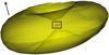 |
Fig. 2. 3D iso-density contours of a simulation of a C-rich donor star with q = 1, f = 80%, and η = 0.8. If Rd = 6 au and Ṁ1 = 3 × 10⁻⁵ M⊙ yr−1, the semitransparent yellow surface surrounds a region where density is larger than 3 × 10⁻¹⁷ g cm−3 and with a diameter of approximately 800 au. The arrow indicates the direction of the orbital angular momentum. A zoom-in on the innermost region is provided in Fig. 3. |
 |
Fig. 3. Zoom-in on the central region in Fig. 2 (black frame) where the donor is a C-rich star and q = 1, f = 80%, and η = 0.8. For Rd = 6 au and Ṁ1 = 3 × 10⁻⁵ M⊙ yr−1, semitransparent yellow represents the 3D iso-density surface ρ = 9 × 10⁻¹⁴ g cm−3 and red corresponds to the surface ρ = 9 × 10⁻¹² g cm−3. The inner boundary of the simulation space is visible in dark red in the right part and the velocity field in the orbital plane is represented. |
Recently, Decin et al. (2019) suggested that the measured mass-loss rates of O-rich intermediate mass AGB stars, coined OH/IR stars, could have been significantly overestimated because of the underlying assumption that the wind was spherically distributed. This preliminary estimate relied on ballistic and hydrodynamic simulations with prescribed acceleration profiles to reproduce different velocity laws (Kim & Taam 2012a; El Mellah & Casse 2017). Here, we introduce a factor to quantify the equatorial density enhancement (EDE) based on a subdivision of the flow in three regions, each spanning a range of colatitudes of π/6 as follows.
– Region A is within a colatitude of π/6 around the axis normal to the orbital plane (the polar axis of our spherical mesh).
– Region C is within a colatitude of π/6 around the orbital plane.
– Region B is in between the other two regions.
Once the flow has reached numerical equilibrium, we averaged the density in regions A and C (and over the 2π longitudinal angles). Then, for each radius, we divided the obtained mean density near the orbital plane by the one near the axis and used the median to obtain the EDE factor, which is represented in Fig. 4. In order to relate this factor to the overestimation of the mass-loss rate, we computed the ratio between the column density of an isotropic wind with a density equal to the one computed in region C and the column density of a wind subdivided in the three uniform regions described above. The results are reported in Fig. 5 and depend on the inclination of the system with respect to the line-of-sight. The wind speed was assumed to be constant so as the density decays as r−2 and then, when the environment is optically thin, the ratio of column densities is a good proxy for the ratio of the measured mass-loss rate assuming spherical symmetry to the real mass-loss rate. We performed this computation for systems seen face-on (in green) and edge-on (in red) by integrating along a line-of-sight either passing by the donor star or offset, such that it intercepts the orbital plane (if face-on) or the orbital axis (if edge-on) with an impact parameter of ∼10 dust condensation radii.
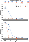 |
Fig. 4. EDE factors for each simulation as a function of η, the ratio of the terminal wind speed to the orbital speed, for a dust condensation radius filling factor of 5% (top) and 80% (bottom). The EDE factors as defined in the text evaluate how the wind is compressed in the orbital plane, with a value of one for a spherically symmetric flow. Different mass ratios (resp. β exponents) are represented with different marker shapes (resp. colors). The solid lines connect the points corresponding to O-rich AGB donor stars. The top axis indicates the corresponding orbital separation for a donor mass of 4 M⊙, a terminal wind speed of 10 km s−1 (with |

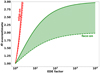 |
Fig. 5. Ratio of the mass-loss rate deduced from assuming spherical symmetry to the real mass-loss rate, as a function of the EDE factor for a system seen face-on (resp. edge-on) in green (resp. red). The solid and dashed lines represent an integration along a line-of-sight that passes by the donor star and offset, respectively. |
In Fig. 5, we see that an EDE factor of unity is associated to a ratio of one (i.e., no overestimation, the real value of the mass-loss rate is obtained). The error remains under a factor of three if the system is seen face-on. The error increases much faster with the EDE factor for systems seen edge-on (approximately proportionally). This computation shows that significant overestimates can occur even for EDE factors as low as a few. The detailed evaluation of the actual overestimation depends on the density profile assumed (Homan et al. 2015, 2016) and on the diagnostics used (either molecular lines or dust emission).
As expected, for circumbinary envelopes that are essentially spherical, the EDE factor is close to one. However, the EDE factor can be much higher when most of the mass is concentrated in the orbital plane. The latter case does occur for realistic parameters. The most direct conclusion we can draw from Fig. 4 is the quick increase in the compression of the flow as soon as the terminal wind speed is slightly lower than the orbital speed. The exact position of the threshold in η depends on the other parameters: The transition occurs at larger values of η for a lower mass ratio and a larger filling factor. While the former evolution corresponds to a larger gravitational influence of the secondary, the latter yields less room for the wind to accelerate, which makes the wind more prone to be shaped by the orbital motion. For a mass ratio of ten and a filling factor of 5%, the wind remains spherical with a compression factor below ten for a terminal wind speed as low as half of the orbital speed (orange markers in top panel in Fig. 4). It is important to take note, however, that such a low ratio η can only be reached in extreme cases, when the orbital period is shorter than a few years (e.g., long period variables from sequence E, Nicholls et al. 2010) or when the wind is anomalously slow.
A general trend to keep in mind is that once the terminal wind speed is slow enough compared to the orbital speed, the compression in the orbital plane is much more efficient for a dust condensation filling factor of 80% (bottom panel) than 5% (top panel). This is due to the fact that the wind speed at the orbital separation can be very low for large filling factors since the acceleration only starts shortly before the wind reaches the secondary. But once η ≳ 2, the compression of the flow is insensitive to the filling factor and to the chemical content of the dust.
Furthermore, these results show that when the filling factor of the dust condensation radius is lower than 10%, little difference should be expected between the compression of the wind around C-rich and O-rich AGB stars. Indeed, by the time the dust-driven wind has reached the secondary, it almost fully reached its terminal wind speed. In this configuration, provided that a C-rich and an O-rich AGB star have the same ratio η of the terminal wind speed to the orbital speed, the morphology of their circumbinary envelope should be similar and no systematic difference should exist. Biases could only be due to different mass ratios between the donor star and the secondary companion. On the contrary, at low η and for a dust condensation radius, which extends up to 80% of the Roche lobe radius of the primary (bottom panel in Fig. 4), the circumbinary envelope around an O-rich star is more prone to being compressed in the orbital plane than for a C-rich star due to the slow acceleration of O-rich winds.
Eventually, it must be noticed that up to a parameter η of two, an EDE factor of three to eight can subsist when the secondary is massive enough (q ≲ 10) and/or when the filling factor is large enough. This implies that mass-loss rate estimates assuming a 1D geometry might significantly overestimate the actual mass-loss rate if the used diagnostic is sensitive to the equatorial density enhancement. As discussed by Decin et al. (2019), mass-loss rates based on dust diagnostics are sensitive to the EDE, while low-excitation CO lines observed with large beams are more reliable tracers of the mass-loss rate even in the case of binary interaction. An additional concern is that the accretion of a fraction of the outflow by the secondary might lower the mass-loss rate measured at larger distance (up to ∼50%, see Sect. 3.3), a contribution which impacts the long term orbital evolution.
3.1.2. Arcs and spiral arms
Spiral arms are a recurrent pattern around cool evolved stars, such as the C-rich AGB stars R Sculptoris (Maercker et al. 2012; Homan et al. 2015) and AFGL3068 (Kim et al. 2017). Arcs have also been observed as broken rings in protoplanetary nebulae by Ramos-Larios et al. (2016), for instance. They have been proposed to originate from expanding outflows collimated in the orbital plane and could be the manifestation of spiral arms seen edge-on (Kim et al. 2019).
The numerous 3D simulations we performed bring about a unique opportunity to disentangle the intrinsic characteristics and the apparent differences induced by the random inclination of the system with respect to the line-of-sight. In these simulations, the spiral shocks in the wind are always seeded in the vicinity of the secondary. However, on a large scale, the details of the flow structure around the secondary do not impact the shape of the circumbinary envelope, which is determined by the dimensionless parameters listed in Sect. 2.2.
A spiral shock is defined by its density enhancement, pitch angle, and vertical extension. The pitch angle is the angle between the spiral and the local direction of the circular orbit; larger pitch angles correspond to more radial spirals (see angle represented in the right panel in Fig. 6). The larger the pitch angle, the larger the ratio is of the inter-arm separation to the orbital separation. When the terminal wind speed is higher than the orbital speed, the pitch angle increases quickly with η (see Kim & Taam 2012b, for a semianalytic formula of the locus of the spiral), although the density contrast and vertical extent eventually vanish. In Fig. 6, slices in the orbital plane of the density are represented for three simulations with a large terminal wind speed compared to the orbital speed, similar to what Cernicharo et al. (2015) found for CW Leo (η = 4). Although they cannot be directly compared to the observations, they are indicative of what a face-on circumbinary envelope might look like in the zero-speed slice of a multichannel molecular line emission map. A first striking result is the independence of the spiral locus once it has been scaled to the orbital separation, with the filling factor and the β exponent. However, the more progressive acceleration of the O-rich AGB star (central panel) blurs the spiral shock which becomes less visible. On the other hand, a C-rich AGB donor star (left panel) can feature a sharp hollow spiral. In the right panel, a zoom-in is shown of the region where the shock first forms for a simulation with a large filling factor C-rich donor star and a higher resolution than the other two panels. A strong instability sets in which propagates along the shock up to large scales. The stability of the Bondi-Hoyle-Lyttleton flow in 3D has been a long-debated question (see Foglizzo et al. 2005, for an overview of the numerical simulations). The different types of instabilities that can be triggered have been identified, such as (i) the flip-flop instability, which is susceptible of producing co- and counter-rotating wind-captured disks alternatively, but which is seemingly absent from 3D simulations (Ruffert 1999; Blondin & Raymer 2012); and (ii) the advective-acoustic instability (Foglizzo et al. 2006), which has been extensively studied in spherical geometry. Here, we do not carry out a detailed analysis of the origin of this instability but point out its quick growth and its capacity to perturb the flow at a large scale.
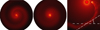 |
Fig. 6. Logarithmic density maps in the orbital plane for three simulations with q = 1 and η = 4. Left panel: C-rich donor star with f = 5%. Center panel: O-rich donor star with f = 80%. Right panel: zoom-in on a C-rich donor star with f = 80%. The white dashed line represents the local tangent to the circle centered on the donor star, while the white dot-dashed line is the local tangent to the spiral shock. Zoom-in for the left and center panels and a zoom-out for the right panel are available in Appendix C. The outer edge of the simulation space lies at 40 orbital separations away from the donor star. |
When the terminal wind speed becomes lower than the orbital speed, the pitch angle significantly decreases as the spiral grows: the wind is not provided with enough kinetic energy per unit mass by the stellar radiative field to overcome the attraction of the Roche potential (η ≲ 1). A significant fraction of the wind fails to reach the outermost shells of the simulation box, which are located at 40 orbital separations (see also Sect. 3.3). As is visible in the high resolution simulation from Fig. 7, the spiral shock stalls, oscillates, breaks apart after a couple of orbital separations, and forms a concentric petal pattern in the orbital plane, even though the orbit is not eccentric and the stellar mass-loss rate is steady. At larger distances, it manifests as arcs in the orbital plane, which propagates outward in a self-similar way, meaning that this morphology could be retrieved at larger distances than 40 orbital separations. At this stage, the propagation is made possible thanks to the pressure support of the inferior layers of the wind. We notice the striking similarity of the flow morphology in Fig. 7, where η = 1, with respect to the zero-speed slice in the molecular line emission maps of CW Leo by Cernicharo et al. (2015). In contrast, using η = 4 leads to the formation of a large pitch angle spiral that is similar to the right panel in Fig. 6. This result leads us to support the proposed low orbital period derived by Decin et al. (2015) rather than the longer one by Cernicharo et al. (2015).
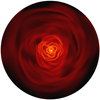 |
Fig. 7. Slice in the orbital plane of the gas density (logarithmic scale) after 20 orbital periods. This simulation is for a C-rich donor star with q = 1, f = 20%, and η = 0.8. An animated version can be found online. The simulation extends up to 40 orbital separations. |
The stalling of the spiral in Fig. 7 does not form a proper circumbinary disk. In Chen et al. (2017), their simulation “M1” with dimensionless parameters that are close to the one in Fig. 7 clearly led to the formation of a ring-like structure at a few orbital separations. We think this difference comes from our simplified treatment of radiative acceleration. The formation of a circumbinary disk is related to a reduced radiative acceleration provoked by an increase of the optical depth (Chen et al. 2020); this is a nonlocal effect that we cannot capture with the present numerical setup.
The flow structure is largely different when seen edge-on. Since its compression in the orbital plane has been described in detail in Sect. 3.1.1, here, we focus on the arcs which emerge as the η parameter decreases. In Fig. 8, we show the density map of the same simulation as the right panel in Fig. 6, but seen from another viewpoint. It is a slice containing the orbital angular momentum vector and the axis joining the two bodies, with the secondary lying on the left of the primary. With an EDE factor of approximately three, the wind compression in the orbital plane is hardly visible by the naked eye in the density distribution. However, monitoring the local mass-loss rate (i.e., per unit solid angle) and comparing it with the isotropic one reveals alternating excesses and deficits (respectively white and green dashed lines) of more than 20%. They are essentially due to an enhanced density and have an opposite phase on the two sides of the secondary. If nonlinear effects are triggered in these regions, such as dust condensation (Boulangier et al. 2019a), these regions might still be visible for an η parameter as large as four. Otherwise, we have to turn toward lower values of η, such as in the bottom panel in Fig. 9. It represents only the inner region, but arcs appear in the flow as slices of a spiral propagating outward (see top panel in the same figure) and spread to much larger distances.
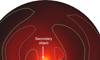 |
Fig. 8. Edge-on view of the simulation in the right panel in Fig. 6. The green and white dashed contours represent 20% deficit and excesses in the local mass-loss rate with respect to the isotropic case, respectively. |
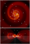 |
Fig. 9. Top panel: logarithmic density map in the orbital plane of the innermost region of the wind. The arrows in white represent the velocity field, while the black lines indicate the streamlines in the vicinity of the secondary where a wind-captured disk develops. Solid white represents the contour of the Roche potential with the value at the innermost Lagrangian point. Bottom panel: side-view of the same density map, with the secondary object to the right of the inner boundary (the red sphere of radius 1.2 dust condensation radius). The velocity field is represented in the upper half, while the mesh and its different levels of refinement are visible in the bottom half. This simulation is for an O-rich donor star with q = 1, f = 80%, and η = 0.8. |
3.2. Innermost region: Wind-captured disks
Roche lobe overflow is a well-known mass transfer mechanism which leads to the formation of a narrow stream of material flowing through the inner Lagrangian point. As the material falls toward the secondary object, it acquires enough angular momentum to form a large and permanent disk within its Roche lobe (see e.g., Frank et al. 1986). Here, we look at a somewhat less extreme case since most cool evolved stars with undetected periodic velocity modulation along the line-of-sight are expected to currently have an orbital separation that is large enough so as to not fill their Roche lobe. At the other end of the possible mass transfer mechanisms lies wind accretion, based on the theory of planar accretion of a supersonic flow by a point-mass (Sect. 8.1 in El Mellah 2016). In our simulations, this regime is an accurate representation of the configurations where the wind speed is much higher than the orbital speed at the orbital separation (i.e., low f and high η). But for wind speeds on the order of the orbital velocity, the wind is strongly beamed toward the secondary and we find a third type of mass transfer called wind-RLOF (Mohamed & Podsiadlowski 2007). Due to the large stellar mass-loss rate and to the focusing of the wind in the orbital plane, a significant mass transfer enhancement can take place compared to the two other regimes. It has been suggested to explain the origin of the excess in barium of some carbon-enhanced metal-poor stars (Abate et al. 2013) and also for the high mass accretion rates needed to reproduce the luminosity of some ultra-luminous X-ray sources (El Mellah et al. 2019b).
Our simulations reproduce the main features associated to the wind-RLOF mechanism: the enhanced mass transfer and the formation of a wind-captured disk around the accretor. In Fig. 9, we show how the wind is strongly shaped by the gravitational potential of the two orbiting bodies in the innermost regions of a wind emitted by an O-rich AGB star. In this configuration, the wind is so slow that when it reaches the secondary, the accretion radius is on the order of the Roche lobe radius of the secondary, which is a clear signature of wind-RLOF. The top panel is a slice in the orbital plane, which is associated to a face-on view, while the bottom panel represents a transverse slice containing the secondary object (to the right of the primary). The velocity field, like in all of the figures in this paper, is the one in the inertial observer frame. While it remains essentially radial around the donor star beyond a few orbital separations, a high vorticity indicative of a wind-captured disk arises in the vicinity of the secondary to the right of the AGB donor in the top panel of Fig. 9. It is important to take notice of the differences between the flow structure in the top panel of this figure or in the zoom-in 3D representation in Fig. 3, and in the right panel in Fig. 6 where the wind was much faster with respect to the orbital speed: The slower wind in Figs. 3 and 9 causes the accretion radius to get larger than the Roche lobe radius. The flow gains enough angular momentum to form a permanent wind-captured disk of maximal extension (Paczynski 1977) and a wide spiral with a low pitch angle in the wake of the accretor.
Furthermore, the wind is now strongly beamed into the orbital plane as is visible in the bottom panel of Fig. 9. Off the plane, the wind fails to take off and falls back, leading to a significant increase in the density scale compared to the configurations where the wind remains essentially isotropic (e.g., Fig. 8). Within this compressed flow, the spiral that is visible in the upper panel deploys and is seen edge-on; it manifests with alternating arcs of higher and lower density.
The presence or lack thereof of a wind-captured disk around the secondary shares another connection with observations. Indeed, provided the secondary has a magnetic field that is large enough, the accretion of matter might not only change the spin of the secondary but also lead to significant outflows (Zanni & Ferreira 2013). Depending on how collimated they are and on the inclination of the magnetic field with respect to the orbital angular momentum axis, it could participate in shaping the low density off-plane environment.
3.3. Mass and angular momentum loss
In this subsection, we report on the fraction of wind which eventually manages to escape the binary system. Due to the preliminary expansion of the donor star, we neglected its spin compared to the much larger orbital angular momentum; however, Chen et al. (2018) carried out a detailed analysis of the orbital shrinking and widening where they also account for spin-orbit synchronization. The secular change of orbital angular momentum induced by the mass-loss of the primary can only provoke a widening or a shrinking of the orbit, sometimes at a rate much higher than the mass loss itself. Constraining the angular momentum loss is a necessary step in performing binary population synthesis and in evaluating which fraction of the systems will undergo a common envelope phase (Ricker & Taam 2012) or produce a Type Ia supernova (Iben & Tutukov 1984; Webbink 1984). Here, given the high stellar mass-loss rate and the large orbital separation, additional sources of orbital angular momentum loss or gain (e.g., magnetic braking, gravitational waves, and stellar expansion) are believed to be minor. If we assume that all the wind either leaves the system or is accreted by the secondary, we have the following evolution for the orbital period P (Tauris & van den Heuvel 2003):
![Mathematical equation: $$ \begin{aligned}&\frac{\dot{P}}{P}=\frac{\dot{M}_1}{M_1}\left[\frac{3\alpha }{1+q}+\frac{q\left(1-\epsilon \right)}{1+q}-3\left(1-\epsilon q\right)\right] \nonumber \\&\quad =\frac{\dot{M}_1}{M_1}\left[\frac{3q^2\left(1-\alpha \right)-2\alpha q-3\left(1-\alpha \right)}{1+q}\right] \end{aligned} $$](/articles/aa/full_html/2020/05/aa37492-20/aa37492-20-eq11.gif) (9)
(9)
where α is the fraction of the wind which escapes the system, while ϵ is the fraction of wind captured by the secondary (also known as the accretion efficiency). The last expression is obtained using α + ϵ = 1. Since Ṁ1 is always negative (the donor star loses mass), the sign of the term within the brackets decides whether the orbit shrinks (if positive) or widens (if negative). In Fig. 10, we represent the opposite of the term within a bracket which, apart from the sign, stands for the ratio of two characteristic time scales: The amount of time for the star to lose a given fraction of its mass to the amount of time for the orbital separation to be modified by the same fraction. In Appendix B and for comparison purposes with other numerical results, we provide the reader with the same graphics for the orbital period and the orbital speed.
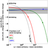 |
Fig. 10. Rate of orbital separation change compared to the rate of stellar mass change. In the gray shaded region, the mass of the donor star changes faster than the orbital separation while above (resp. below) the orbit expands (resp. contracts). The two limit cases are conservative mass transfer (dotted line, RLOF) and pure mass loss without accretion by the secondary (solid blue line). In-between, the solid green and red lines are for an accretion efficiency by the secondary of 5% and 50%, respectively. The arrows indicate that as mass transfer proceeds, the mass ratio can only decrease. |
The mass-loss rate Ṁ1 is highly variable during the evolution of AGB stars, with short episodes of enhanced mass loss up to 10−5 M⊙ yr−1, which are separated by quiescent phases where the mass-loss rate is on the order of 10−7 M⊙ yr−1 (Bloecker 1995). In this context, the reader should keep in mind that the time scales involved in the ratio represented in Fig. 10 are bound to change by order of magnitudes during the AGB phase and should be thought of as instantaneous rates of change. Within the gray shaded region, the rate of change of the orbital separation is lower than the rate of change of the mass of the donor star while elsewhere, for a given relative change of the donor mass by a certain fraction, the orbital separation changes by more than this fraction (i.e., the orbital separation evolves “faster” than the donor mass). Not surprisingly, for a mass ratio q = M1/M2 lower than unity, the orbital separation evolves slowly. Indeed, since most of the mass is now in the secondary, the total mass remains fairly constant as the primary loses mass and the impact of the mass loss on the orbit is limited.
The two asymptotic cases are the black dotted line (RLOF, ϵ = 1) and the solid blue line (free wind, α = 1). Arguments based on a polytropic representation of the equation-of-state of the donor star show that for q ∼ 1, a purely conservative mass transfer (i.e., ϵ = 1 so α = 0) is prone to provoke a faster contraction of the Roche lobe radius than of the stellar radius (D’Souza et al. 2005). The positive feedback loop provokes the quick inspiral of the two bodies and the system enters a common envelope phase, although properly accounting for the stellar internal structure pushes the critical mass ratio to a few units (Pavlovskii et al. 2017; Quast et al. 2019). These results are consistent with the present framework when mass transfer is only partly conservative (α < 1, black dotted line, red and green solid lines in Fig. 10): we see in Fig. 10 that there is always a critical mass ratio beyond which the mass transfer yields a quick inspiral from the system (compared to the mass-loss time scale). The less conservative the mass transfer, the larger this critical mass ratio is.
We measured α by computing the mass-loss rate at ten orbital separations and by comparing it to the mass-loss rate at the inner edge of the simulation space, which is representative of the stellar mass-loss rate. In Fig. 11, we plotted ϵ = 1 − α as a function of the main parameter, the ratio η of the terminal wind speed to the orbital speed. Beyond η = 1, the accretion efficiency remains invariably lower than 5%. Negative values are due to unsteadiness and uncertainties in the numerical computation on the order of a few percent. This uncertainty precludes any quantitative prediction, but relying on Fig. 10 provides insightful predictions. According to these results, for a mass ratio inferior than ten, a terminal wind speed higher than the orbital speed means that the orbital separation remains essentially unchanged over the mass-loss time scale M1/Ṁ1 (although the orbital period might increase significantly, see upper panel in Fig. B.1). In the same way, even for η < 1, the orbital evolution of binaries where the donor star is a C-rich AGB star that is ten times more massive than the secondary (orange squares) can only be modest, and so is the orbital evolution of O-rich AGB stars with q = 10 provided the dust condensation filling factor is lower than ∼20% (orange circles in the upper panel). For f = 80%, the wind from O-rich AGB stars is significantly captured by the secondary when η < 1 due to the wind-RLOF regime, leading to accretion efficiency of several tens of percent. Provided the mass ratio is high (q higher than a few units), the orbital separation quickly decays until the mass ratio is low enough to enter the gray shaded region in Fig. 10. When q is higher than a few units, the associated quick increase of the orbital speed enhances the phenomenon by lowering η and increasing the accretion efficiency ϵ. In the same way, even for a low filling factor, a massive secondary object (q = 1) captures a significant fraction of the stellar wind, but due to the low mass ratio, Fig. 10 indicates that the orbit only marginally changes over a mass-loss characteristic time scale.
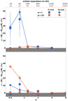 |
Fig. 11. Fraction ϵ of the wind captured by the secondary (accretion efficiency) as a function of the ratio η of the terminal wind speed to the orbital speed for a dust condensation radius filling factor of 5% (upper panel) and 80% (lower panel). Square (resp. circular) markers are for C-rich (resp. O-rich) AGB stars. Blue (resp. orange) markers are for mass ratios of q = 1 (resp. q = 10). The results for O-rich stars are connected with solid lines and the error bars represent the variations over a dynamical time scale. The top scale is the same as in Fig. 4. |
4. Discussion and summary
With our numerical setup, we recover a wide variety of observed circumstellar morphologies produced by the presence of a lower mass companion around a mass losing cool evolved star. We show that the main parameter driving the wind dynamics is the ratio η of the terminal wind speed to the orbital speed, although significant differences can arise between C-rich and O-rich stars for η ∼ 1 when the dust condensation region extends up to 80% of the Roche lobe radius of the donor star. These numerical simulations confirm that the observation of alternating higher and lower density arcs or of a spiral pattern are indicative of an edge-on or a face-on inclination of the orbit with respect to the line-of-sight, respectively. We also computed the amplitude of the wind compression in the orbital plane for each set of parameters. It shows that beyond a mass ratio of ten, the wobbling motion of the primary induced by the secondary is not large enough to significantly flatten the wind, except for a high dust condensation filling factor of 80% and a very low ratio η of 0.5, which is only realistic if the orbital period is less than a decade. Assuming the orbital angular momentum only changes due to the outflow from the cool evolved star, we identified the following three necessary conditions in order to observe a significant shrinking of the orbit over a mass-loss time scale:
-
a terminal wind speed lower than the orbital speed,
-
a mass ratio higher than one or two, and
-
a dust condensation region which extends up to several tens of percent of the primary Roche lobe radius.
In the other cases, the system will undergo a variation in the orbital separation that is of a lower relative change than the stellar mass change, thus either an orbit widening or shrinking depending on the mass ratio and on the fraction of stellar wind captured by the secondary. Accounting for eccentricity will likely modify these conclusions. Eccentric orbits have been commonly observed for systems with large orbital separations (i.e., large values of η), which is in agreement with the long circularization time scales expected (Zahn 1977). Its effect on the wind morphology has been thoroughly reported on in Kim et al. (2015, 2017), and Kim et al. (2019), but to our knowledge, its impact on the orbital angular momentum has yet to be investigated.
In the configurations where q ∼ 1 and the orbital speed is similar or higher than the terminal wind speed (η ≲ 1), we observed the emergence of an unstable flow where the pitch angle of the spiral is cancelled out within a couple of orbital separations. The shell fragments and is eventually ejected by the incoming material, producing a concentric petal pattern in the orbital plane that is reminiscent of what is observed around the C-rich AGB star CW Leo (Decin et al. 2015; Cernicharo et al. 2015). Most material is concentrated in the orbital plane due to the low value of η, so a slice in the orbital plane of the simulation should be representative of a face-on view. Interestingly enough, these successive arcs in the orbital plane appear in spite of the steadiness of the mass-loss rate, without any burst or pulsation. The spacing between them is on the order of a few orbital separations at the outer edge of our simulation box and expands self-similarly with the distance to the donor star in the outer regions.
Unfortunately, the long orbital periods of binaries containing a cool evolved star preclude any monitoring of the rate of change of the orbital period. But in systems with shorter orbital periods, such as supergiant X-ray binaries and ultra-luminous X-ray sources, this rate has been measured (see e.g., Falanga et al. 2015). The mass ratio can then be constrained using the wobbling motion of the two bodies projected along the line-of-sight (see e.g., Quaintrell et al. 2003) or the timing of the neutron star pulses (Fürst et al. 2018). Together, they bring strong constraints on the wind fraction ϵ captured by the secondary and can be compared to the mass accretion rates deduced from the X-ray luminosity.
This paper introduces a convenient framework to implement new effects. In particular, the spherical mesh centered on the donor star opens the door to the addition of a key-ingredient: matter-radiation interaction. In this paper, we simply parametrized the wind acceleration to identify archetypal configurations. A subset of configurations can now serve as the bedrock for more realistic simulations where additional physical effects are introduced, such as the growth of dust grains and their coupling with the stellar radiative field. Thanks to the low computational cost of each simulation and to innovative schemes to treat parabolic and elliptic equations that have recently been implemented in MPI-AMRVAC (Teunissen & Keppens 2019), we can start to explore radiative effects.
Each of the simulations we performed, which contain information on the temperature, gas density, and velocity 3D distribution, can now be post-processed to produce synthetic emission maps for different inclinations. In order to produce molecular-line emission maps, we need to use molecular abundance profiles, such as the one computed by Van de Sande et al. (2019), and new-generation radiative transfer codes, such as Magritte (De Ceuster et al. 2019).
Supplementary Material
Movie of Fig. 7 Access Supplementary Material
Acknowledgments
The authors thank the anonymous referee for her/his insights. The authors wish to thank the ATOMIUM ALMA Large Programme collaboration (2018.1.00659, PI. L. Decin) for the observational consequences of the present analysis. IEM has received funding from the Research Foundation Flanders (FWO) and the European Union’s Horizon 2020 research and innovation program under the Marie Skłodowska-Curie grant agreement No 665501. LD, JB and WD acknowledge support from the ERC consolidator grant 646758 AEROSOL. The simulations were conducted on the Tier-1 VSC (Flemish Supercomputer Center funded by Hercules foundation and Flemish government). RK is supported by Internal Funds KU Leuven, project C14/19/089 TRACESpace.
References
- Abate, C., Pols, O. R., Izzard, R. G., Mohamed, S. S., & de Mink, S. E. 2013, A&A, 552, A26 [NASA ADS] [CrossRef] [EDP Sciences] [Google Scholar]
- Bermúdez-Bustamante, L. C., García-Segura, G., Steffen, W., & Sabin, L. 2020, MNRAS, 493, 2606 [NASA ADS] [CrossRef] [Google Scholar]
- Bidelman, W. P., & Keenan, P. C. 1951, ApJ, 114, 473 [NASA ADS] [CrossRef] [Google Scholar]
- Bloecker, T. 1995, A&A, 297, 727 [Google Scholar]
- Blondin, J. M., & Raymer, E. 2012, ApJ, 752, 30 [NASA ADS] [CrossRef] [Google Scholar]
- Blondin, J. M., Stevens, I. R., & Kallman, T. R. 1991, ApJ, 371, 684 [NASA ADS] [CrossRef] [Google Scholar]
- Boulangier, J., Clementel, N., Van Marle, A. J., Decin, L., & De Koter, A. 2019a, MNRAS, 482, 5052 [NASA ADS] [CrossRef] [Google Scholar]
- Boulangier, J., Gobrecht, D., Decin, L., de Koter, A., & Yates, J. 2019b, MNRAS, 489, 4890 [NASA ADS] [CrossRef] [Google Scholar]
- Bowen, G. H. 1988, ApJ, 329, 299 [NASA ADS] [CrossRef] [Google Scholar]
- Bujarrabal, V., Castro-Carrizo, A., Alcolea, J., et al. 2016, A&A, 593, A92 [NASA ADS] [CrossRef] [EDP Sciences] [Google Scholar]
- Cernicharo, J., Marcelino, N., Agúndez, M., & Guélin, M. 2015, A&A, 575, A91 [NASA ADS] [CrossRef] [EDP Sciences] [Google Scholar]
- Chen, Z., Frank, A., Blackman, E. G., Nordhaus, J., & Carroll-Nellenback, J. 2017, MNRAS, 468, 4465 [NASA ADS] [CrossRef] [Google Scholar]
- Chen, Z., Blackman, E. G., Nordhaus, J., Frank, A., & Carroll-Nellenback, J. 2018, MNRAS, 473, 747 [NASA ADS] [CrossRef] [Google Scholar]
- Chen, Z., Ivanova, N., & Carroll-Nellenback, J. 2020, ApJ, 892, 110 [NASA ADS] [CrossRef] [Google Scholar]
- Chita, S. M., Langer, N., Van Marle, J., García-Segura, G., & Heger, A. 2008, A&A, 488, L37 [NASA ADS] [CrossRef] [EDP Sciences] [Google Scholar]
- Claeys, J. S., Pols, O. R., Izzard, R. G., Vink, J., & Verbunt, F. W. 2014, A&A, 563, A83 [NASA ADS] [CrossRef] [EDP Sciences] [Google Scholar]
- De Ceuster, F., Homan, W., Boyle, P., Hetherington, J., & Yates, J. 2019, MNRAS, 492, 1812 [Google Scholar]
- De Marco, O., & Izzard, R. G. 2017, Dawes Review 6: The Impact of Companions on Stellar Evolution (Cambridge University Press) [Google Scholar]
- de Val-Borro, M., Karovska, M., Sasselov, D. D., & Stone, J. M. 2017, MNRAS, 468, 3408 [NASA ADS] [CrossRef] [Google Scholar]
- Decin, L., Hony, S., De Koter, A., et al. 2006, A&A, 456, 549 [NASA ADS] [CrossRef] [EDP Sciences] [Google Scholar]
- Decin, L., De Beck, E., Brünken, S., et al. 2010a, A&A, 516, A69 [NASA ADS] [CrossRef] [EDP Sciences] [Google Scholar]
- Decin, L., Justtanont, K., De Beck, E., et al. 2010b, A&A, 521, A1 [NASA ADS] [CrossRef] [EDP Sciences] [Google Scholar]
- Decin, L., Richards, A. M. S., Neufeld, D., et al. 2015, A&A, 574, A5 [NASA ADS] [CrossRef] [EDP Sciences] [Google Scholar]
- Decin, L., Richards, A. M., Danilovich, T., Homan, W., & Nuth, J. A. 2018, A&A, 615, A28 [NASA ADS] [CrossRef] [EDP Sciences] [Google Scholar]
- Decin, L., Homan, W., Danilovich, T., et al. 2019, Nat. Astron., 3, 408 [NASA ADS] [CrossRef] [Google Scholar]
- Dell’Agli, F., García-Hernández, D. A., Ventura, P., et al. 2015, MNRAS, 454, 4235 [NASA ADS] [CrossRef] [Google Scholar]
- D’Souza, M. C. R., Motl, P. M., Tohline, J. E., & Frank, J. 2005, ApJ, 643, 381 [Google Scholar]
- Edgar, R. G. 2004, New Astron. Rev., 48, 843 [NASA ADS] [CrossRef] [Google Scholar]
- Eggleton, P. P. 1983, ApJ, 268, 368 [NASA ADS] [CrossRef] [Google Scholar]
- El Mellah, I. 2016, Ph.D. Thesis [Google Scholar]
- El Mellah, I., & Casse, F. 2015, MNRAS, 454, 2657 [NASA ADS] [CrossRef] [Google Scholar]
- El Mellah, I., & Casse, F. 2017, MNRAS, 467, 2585 [NASA ADS] [Google Scholar]
- El Mellah, I., Sundqvist, J. O., & Keppens, R. 2018, MNRAS, 475, 3240 [NASA ADS] [CrossRef] [Google Scholar]
- El Mellah, I., Sander, A. A. C., Sundqvist, J. O., & Keppens, R. 2019a, A&A, 622, A189 [NASA ADS] [CrossRef] [EDP Sciences] [Google Scholar]
- El Mellah, I., Sundqvist, J. O., & Keppens, R. 2019b, A&A, 622, L3 [NASA ADS] [CrossRef] [EDP Sciences] [Google Scholar]
- Falanga, M., Bozzo, E., Lutovinov, A., et al. 2015, A&A, 577, A130 [NASA ADS] [CrossRef] [EDP Sciences] [Google Scholar]
- Foglizzo, T., Galletti, P., & Ruffert, M. 2005, A&A, 435, 397 [NASA ADS] [CrossRef] [EDP Sciences] [Google Scholar]
- Foglizzo, T., Galletti, P., Scheck, L., & Janka, H. T. 2006, ApJ, 654, 29 [Google Scholar]
- Frank, J., King, A., & Raine, D. J. 1986, Phys. Today, 39, 124 [CrossRef] [Google Scholar]
- Freytag, B., Liljegren, S., & Höfner, S. 2017, A&A, 600, A137 [NASA ADS] [CrossRef] [EDP Sciences] [Google Scholar]
- Fürst, F., Walton, D. J., Heida, M., et al. 2018, A&A, 616, A186 [NASA ADS] [CrossRef] [EDP Sciences] [Google Scholar]
- Gobrecht, D., Cherchneff, I., Sarangi, A., Plane, J. M., & Bromley, S. T. 2016, A&A, 585, A6 [NASA ADS] [CrossRef] [EDP Sciences] [Google Scholar]
- Groenewegen, M. A. 2012, A&A, 543, A36 [NASA ADS] [CrossRef] [EDP Sciences] [Google Scholar]
- Groenewegen, M. A., Sevenster, M., Spoon, H. W., & Pérez, I. 2002, A&A, 390, 511 [NASA ADS] [CrossRef] [EDP Sciences] [Google Scholar]
- Habing, H. J., & Olofsson, H. 2003, Asymptotic Giant Branch Stars (New York, Berlin: Springer) [Google Scholar]
- Herwig, F. 2005, ARA&A, 43, 435 [NASA ADS] [CrossRef] [Google Scholar]
- Herwig, F., & Austin, S. M. 2004, ApJ, 613, L73 [NASA ADS] [CrossRef] [Google Scholar]
- Höfner, S., & Olofsson, H. 2018, A&ARv, 26, 1 [NASA ADS] [CrossRef] [Google Scholar]
- Höfner, S., Bladh, S., Aringer, B., & Ahuja, R. 2016, A&A, 594, A108 [NASA ADS] [CrossRef] [EDP Sciences] [Google Scholar]
- Homan, W., Decin, L., de Koter, A., et al. 2015, A&A, 579, A118 [NASA ADS] [CrossRef] [EDP Sciences] [Google Scholar]
- Homan, W., Boulangier, J., Decin, L., & De Koter, A. 2016, A&A, 596, A91 [NASA ADS] [CrossRef] [EDP Sciences] [Google Scholar]
- Homan, W., Richards, A., Decin, L., De Koter, A., & Kervella, P. 2018, A&A, 616, A34 [NASA ADS] [CrossRef] [EDP Sciences] [Google Scholar]
- Huarte-Espinosa, M., Carroll-Nellenback, J., Nordhaus, J., Frank, A., & Blackman, E. G. 2013, MNRAS, 433, 295 [NASA ADS] [CrossRef] [Google Scholar]
- Iben, I. J., & Tutukov, A. V. 1984, ApJS, 54, 335 [NASA ADS] [CrossRef] [Google Scholar]
- Jofré, P., Jorissen, A., Van Eck, S., et al. 2016, A&A, 595, A60 [NASA ADS] [CrossRef] [EDP Sciences] [Google Scholar]
- Kamath, D., Wood, P. R., Van Winckel, H., & Nie, J. D. 2016, A&A, 586, L5 [NASA ADS] [CrossRef] [EDP Sciences] [Google Scholar]
- Keppens, R. 1997, A&A, 318, 275 [NASA ADS] [Google Scholar]
- Keppens, R., Solanki, S. K., & Charbonnel, C. 2000, A&A, 359, 552 [NASA ADS] [Google Scholar]
- Khouri, T., De Koter, A., Decin, L., et al. 2014, A&A, 561, A5 [NASA ADS] [CrossRef] [EDP Sciences] [Google Scholar]
- Khouri, T., Maercker, M., Waters, L. B., et al. 2016, A&A, 591, A70 [NASA ADS] [CrossRef] [EDP Sciences] [Google Scholar]
- Kim, H., & Taam, R. E. 2012a, ApJ, 759, 59 [NASA ADS] [CrossRef] [Google Scholar]
- Kim, H., & Taam, R. E. 2012b, ApJ, 744, 136 [NASA ADS] [CrossRef] [Google Scholar]
- Kim, H., Liu, S. Y., Hirano, N., et al. 2015, ApJ, 814, 1 [NASA ADS] [CrossRef] [Google Scholar]
- Kim, H., Trejo, A., Liu, S. Y., et al. 2017, Nat. Astron., 1, 0060 [NASA ADS] [CrossRef] [Google Scholar]
- Kim, H., Liu, S.-Y., & Taam, R. E. 2019, ApJS, 243, 35 [NASA ADS] [CrossRef] [Google Scholar]
- Knapp, G. R., Young, K., Lee, E., & Jorissen, A. 1998, ApJS, 117, 209 [NASA ADS] [CrossRef] [Google Scholar]
- Lamers, H. J. G. L. M., & Cassinelli, J. P. 1999, Introduction to Stellar Winds (Cambridge Univ. Press) [CrossRef] [Google Scholar]
- Leisenring, J. M., Kemper, F., & Sloan, G. C. 2008, ApJ, 681, 1557 [NASA ADS] [CrossRef] [Google Scholar]
- Levesque, E. M. 2010, New Astron. Rev., 54, 1 [NASA ADS] [CrossRef] [Google Scholar]
- Liljegren, S., Höfner, S., Nowotny, W., & Eriksson, K. 2016, A&A, 589, A130 [NASA ADS] [CrossRef] [EDP Sciences] [Google Scholar]
- Liu, Z.-W., Stancliffe, R. J., Abate, C., & Matrozis, E. 2017, ApJ, 846, 117 [NASA ADS] [CrossRef] [Google Scholar]
- Maercker, M., Mohamed, S., Vlemmings, W. H. T., et al. 2012, Nature, 490, 232 [NASA ADS] [CrossRef] [PubMed] [Google Scholar]
- Marshall, J. R., Van Loon, J. T., Matsuura, M., et al. 2004, MNRAS, 355, 1348 [NASA ADS] [CrossRef] [Google Scholar]
- Mastrodemos, N., & Morris, M. 1999, ApJ, 523, 357 [NASA ADS] [CrossRef] [Google Scholar]
- Moe, M., & Di Stefano, R. 2017, ApJS, 230, 15 [Google Scholar]
- Mohamed, S., & Podsiadlowski, P. 2007, Wind Roche-Lobe Overflow: a New Mass-Transfer Mode for Wide Binaries (San Francisco: ASP) [Google Scholar]
- Mohamed, S., & Podsiadlowski, P. 2011, ASP Conf. Ser., 445 [Google Scholar]
- Nicholls, C. P., Wood, P. R., & Cioni, M.-R. R. 2010, MNRAS, 405, 1770 [NASA ADS] [Google Scholar]
- Nordhaus, J., & Blackman, E. G. 2006, MNRAS, 370, 2004 [NASA ADS] [CrossRef] [Google Scholar]
- Paczynski, B. 1977, ApJ, 216, 822 [NASA ADS] [CrossRef] [Google Scholar]
- Pavlovskii, K., Ivanova, N., Belczynski, K., & Van, K. X. 2017, MNRAS, 465, 2092 [NASA ADS] [CrossRef] [Google Scholar]
- Porth, O., Xia, C., Hendrix, T., Moschou, S. P., & Keppens, R. 2014, ApJS, 214, 4 [Google Scholar]
- Quaintrell, H., Norton, A. J., Ash, T. D. C., et al. 2003, A&A, 401, 313 [NASA ADS] [CrossRef] [EDP Sciences] [Google Scholar]
- Quast, M., Langer, N., & Tauris, T. M. 2019, A&A, 628, A19 [NASA ADS] [CrossRef] [EDP Sciences] [Google Scholar]
- Ramos-Larios, G., Santamaría, E., Guerrero, M. A., et al. 2016, MNRAS, 462, 610 [NASA ADS] [CrossRef] [Google Scholar]
- Ramstedt, S., Mohamed, S., Vlemmings, W. H., et al. 2014, A&A, 570, L14 [NASA ADS] [CrossRef] [EDP Sciences] [Google Scholar]
- Ramstedt, S., Schöier, F. L., & Olofsson, H. 2009, A&A, 499, 515 [NASA ADS] [CrossRef] [EDP Sciences] [Google Scholar]
- Ricker, P. M., & Taam, R. E. 2012, ApJ, 746, 74 [NASA ADS] [CrossRef] [Google Scholar]
- Ruffert, M. 1999, A&A, 346, 861 [NASA ADS] [Google Scholar]
- Saladino, M. I., Pols, O., & Abate, C. 2019, A&A, 626, A68 [NASA ADS] [CrossRef] [EDP Sciences] [Google Scholar]
- Sargent, B. A., Srinivasan, S., & Meixner, M. 2011, ApJ, 728, 93 [NASA ADS] [CrossRef] [Google Scholar]
- Shklovsky, I. S. 1956, AZh, 33, 315 [Google Scholar]
- Straniero, O., Chieffi, A., Limongi, M., et al. 1997, ApJ, 478, 332 [NASA ADS] [CrossRef] [Google Scholar]
- Tauris, T. M., & van den Heuvel, E. 2003, Formation and evolution of compact stellar X-ray sources (Cambridge University Press) [Google Scholar]
- Teunissen, J., & Keppens, R. 2019, Comput. Phys. Commun., 245, 106866 [CrossRef] [Google Scholar]
- Toro, E. F., Spruce, M., & Speares, W. 1994, Shock Waves, 4, 25 [NASA ADS] [CrossRef] [EDP Sciences] [Google Scholar]
- Van de Sande, M., Walsh, C., Mangan, T. P., & Decin, L. 2019, MNRAS, 2041, 2023 [NASA ADS] [CrossRef] [Google Scholar]
- Vreugdenhil, C. B., & Koren, B. 1993, Numerical Methods for Advection-Diffusion Problems (Vieweg), 373 [Google Scholar]
- Webbink, R. F. 1984, ApJ, 277, 355 [NASA ADS] [CrossRef] [Google Scholar]
- Xia, C., Teunissen, J., El Mellah, I., Chané, E., & Keppens, R. 2018, ApJS, 234, 30 [Google Scholar]
- Yang, M., Bonanos, A. Z., Jiang, B. W., et al. 2018, A&A, 616, A175 [NASA ADS] [CrossRef] [EDP Sciences] [Google Scholar]
- Zahn, J.-P. 1977, A&A, 57, 383 [NASA ADS] [Google Scholar]
- Zanni, C., & Ferreira, J. 2013, A&A, 550, A99 [NASA ADS] [CrossRef] [EDP Sciences] [Google Scholar]
Appendix A: Dust-driven wind velocity profiles
Beyond the observational motivations given in Sects. 2.1.1 and 2.2, in this appendix, we propose semianalytic arguments which enable one to get an estimate of the shape of the velocity profile for an isolated isotropic dust-driven wind. We fit the obtained velocity profiles with β-laws and discuss the legitimacy of our underlying assumption of representing the wind acceleration based on a predefined β velocity profile for C-rich and O-rich AGB stars.
It is possible to determine the velocity profile v for a given opacity profile by numerically integrating the steady 1D spherical equation of motion for a pressureless gas:
 (A.1)
(A.1)
where we normalized the length to the dust condensation radius and the speed to the escape speed at the dust condensation radius. We note that Γ is a constant similar to the Eddington parameter, but with an opacity of κ0, which is defined below:
 (A.2)
(A.2)
with M⋆ representing the mass of the star, L⋆ is the luminosity of the star, c corresponds to the speed of light, and G is the gravitational constant. The effective opacity κ0 encapsulates the normalization of the dust opacity and the coupling between the dust and the gas, which determines which fraction of the momentum provided to the dust is eventually deposited in the gas. It is typically much higher than the dust-free gas opacity.
For C-rich outflows, the dust species responsible for the wind acceleration are better identified and are more rarer. A dimensionless opacity profile κ(r) introduced by Bowen (1988) and commonly invoked to mimic the dust growth in C-rich winds and compute the dust-driven acceleration (see e.g., Chen et al. 2020; Bermúdez-Bustamante et al. 2020) is:
 (A.3)
(A.3)
where Tc is the dust condensation temperature and ΔT stands for a range of temperature where the grains grow. For an isolated star, the equilibrium temperature profile of the gas is given by the geometrical dilution factor:
![Mathematical equation: $$ \begin{aligned} T\left(r\right) = \frac{T_{\star }}{2}\left[1-\sqrt{1-\left(\frac{R_{\star }}{r}\right)^2}\right]^{1/4} \end{aligned} $$](/articles/aa/full_html/2020/05/aa37492-20/aa37492-20-eq15.gif) (A.4)
(A.4)
with T⋆ representing the stellar effective temperature and R⋆ is the stellar radius. For a C-rich wind, κ0∼5–10 g cm−2 (Bermúdez-Bustamante et al. 2020). For an AGB star with a mass of M1 = 1 M⊙, a radius of R1 = 300 R⊙, and an effective temperature of T1 = 2500 K, we get Γ ∼ 2. We are now in a position to solve the equation of motion numerically (A.1) for a C-rich wind with a dust condensation temperature of Tc = 1500 K and ΔT = 60 K (Leisenring et al. 2008). We obtained the solid blue line shown in Fig. A.1, which is remarkably well fit by a β-law with β ∼ 0.6 (dashed blue line). The agreement between the two fully justifies the simplified prescription we relied on to compute wind acceleration of C-rich winds.
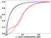 |
Fig. A.1. Velocity profiles obtained by solving the pressureless isotropic equation of motion (A.1) for empirical opacity profiles (solid lines), for both a C-rich (blue) and an O-rich AGB star (red). The dashed lines are the corresponding fits with β-laws, with β ∼ 0.6 (C-rich) and β ∼ 5 (O-rich). |
To our knowledge, there is currently no ab initio computation of O-rich wind acceleration, partly because we do not know how the monomers form and which molecule clusters will be the first to coagulate into dust grains (Boulangier et al. 2019b,a). In order to obtain a physically-motivated opacity profile, we would need a proper treatment for the dust formation and growth based on a state-of-the-art chemical network, along with a radiative transfer solver. Tuning the parameters above, we could never get a velocity profile which could be fit by a β-law with β > 1 for realistic values. An alternative is to consider an acceleration, which is mostly driven by two dust species, indexed 1 and 2. The first species to condensate at a temperature Tc, 1, dust #1, has an opacity that is high enough to drive an outflow, but only marginally, to prevent the solution from converging toward a low β profile similar to the C-rich one. It is enough to lift the wind up to a distance where dust #2, with a condensation temperature of Tc, 2 < Tc, 1, condensates. Dust #2 has an opacity that is high enough to prevent the wind from falling back and to drive a proper wind. The total opacity is now given by:
 (A.5)
(A.5)
where α is a constant that stands for the relative capacity of dust #1 to drive the wind compared to dust #2. We carried out the computation for the same stellar parameters but with α = 2% and κ0 = 400 g cm−2, which corresponds to Γ ∼ 100, such that the initial acceleration is marginally positive. Around O-rich AGB stars, dust based on aluminum and silicium are expected to contribute to wind driving and they can play the role of dust#1 and #2, respectively, which motivates Tc, 1 = 1800 K, Tc, 2 = 500 K. This computation leads to the solid red velocity profile in Fig. A.1 and to a fit by a β-law with β ∼ 5 (dashed red line).
Due to the two separated components of the opacity, fitting the velocity profile obtained for an O-rich wind with a single β-law gives a much poorer fit than for a C-rich wind, especially in the innermost region. However, in this region, the preliminary simulations that we carried out, including realistic AGB pulsations and a chemical network, indicate that pulsations still contribute to lifting the wind up to several dust condensation radii. It makes the inner region turbulent and prevents from obtaining realistic velocity profiles based on the opacity profile alone. Because we did not model the pulsations in our simulations, we instead rely on a β = 5 velocity profile.
Although the acceleration profiles that we derived from beta-laws will differ from the ones inferred in the future from first principles, they are compatible with the models and observations at our disposal and they are sufficient at capturing the wind dynamics as it develops beyond the orbital scale.
Appendix B: Orbital separation changes due to mass loss
If the orbital separation increases as the system loses mass, the orbital period increases. And if the orbital period decreases as the system loses mass, the orbital separation decreases. However, mixed cases can occur. Since the total mass of the system diminishes if the orbital separation decreases slowly, the orbital period can increase. Comparing Fig. 10 and the upper panel in Fig. B.1 confirms that when the mass ratio is such that (ȧ/a)/(−Ṁ1/M1) is negative (i.e., the orbit is shrinking), yet close to zero, the orbital period can still be increasing. The net effect on the orbital speed is visible in the bottom panel of Fig. B.1.
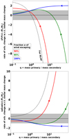 |
Fig. B.1. Rate of change of the orbital period (upper panel) and orbital speed aΩ (bottom panel) compared to the rate of stellar mass change. In the gray shaded region, the mass of the donor star changes faster than the orbital period or speed. The two limit cases are the conservative mass transfer (dotted line, RLOF) and the pure mass loss without accretion by the secondary (solid blue line). In between, the green and red solid lines correspond to an accretion efficiency by the secondary of 5% and 50%, respectively. The arrows indicate that as mass transfer proceeds, the mass ratio can only decrease. |
Appendix
The figures displayed in the following pages represent 2D slices of the density map for each set of the 59 simulations. As explained in Sect. 2.3, in the 13 remaining simulations, the presence of the secondary has essentially no impact on the morphology of the wind, which remains isotropic. The density is given in units of the density at the sonic point, which is really close to the density at the dust condensation radius. Each simulation is labeled with a tag, which contains all of the parameters used for the simulation. The number that follows the letter “q” is the mass ratio, the filling factor is given after the letter “f” in %, after the letter “e” is the result of the ratio η multiplied by ten, and the final letter (“C” or “O”) indicates the value of the β exponent (0.1 or 5, respectively).
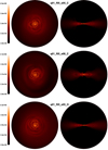 |
Fig. C.1. Slices of the density, in units of the density at the sonic point, in the orbital plane (left column), and in the plane containing the orbital axis and the line joining the two bodies (right column) for unsteady configurations. Labels give the parameters used (see text for more details). The simulations extend up to 40 orbital separations. |
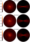 |
Fig. C.1. continued. |
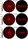 |
Fig. C.1. continued. |
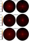 |
Fig. C.2. Slices of the density in units of the density at the sonic point, in the orbital plane (left column), and in the plane containing the orbital axis and the line joining the two bodies (right column) for spiral and arc configurations. Labels give the parameters used (see text for more details). The simulations extend up to 40 orbital separations. |
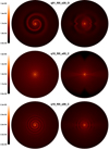 |
Fig. C.2. continued. |
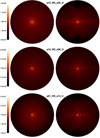 |
Fig. C.2. continued. |
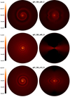 |
Fig. C.2. continued. |
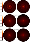 |
Fig. C.2. continued. |
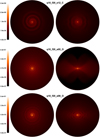 |
Fig. C.2. continued. |
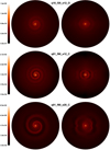 |
Fig. C.2. continued. |
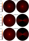 |
Fig. C.2. continued. |
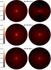 |
Fig. C.2. continued. |
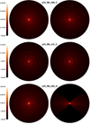 |
Fig. C.2. continued. |
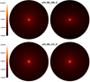 |
Fig. C.2. continued. |
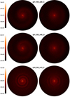 |
Fig. C.3. Slices of the density in units of the density at the sonic point, in the orbital plane (left column), and in the plane containing the orbital axis and the line joining the two bodies (right column) for isotropic configurations. Labels give the parameters used (see text for more details). The simulations extend up to 40 orbital separations. |
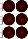 |
Fig. C.3. continued. |
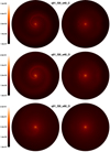 |
Fig. C.3. continued. |
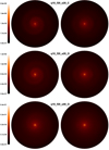 |
Fig. C.3. continued. |
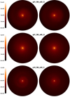 |
Fig. C.3. continued. |
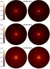 |
Fig. C.3. continued. |
All Tables
All Figures
|
Fig. 1. Velocity profiles for a C-rich AGB star (solid blue line, β = 0.1) and for an O-rich AGB star (solid red line, β = 5), from 1.2 to 500 dust condensation radii. The red dashed line represents the modified β-law such that the wind is launched at a velocity slightly above the sound speed at the inner edge of the simulation space (β′ ∼ 6.7). The sound speed profile is the dotted black line and we assumed a fiducial terminal wind speed that is four times higher than the sound speed at the dust condensation radius. |
| In the text | |
|
Fig. 2. 3D iso-density contours of a simulation of a C-rich donor star with q = 1, f = 80%, and η = 0.8. If Rd = 6 au and Ṁ1 = 3 × 10⁻⁵ M⊙ yr−1, the semitransparent yellow surface surrounds a region where density is larger than 3 × 10⁻¹⁷ g cm−3 and with a diameter of approximately 800 au. The arrow indicates the direction of the orbital angular momentum. A zoom-in on the innermost region is provided in Fig. 3. |
| In the text | |
|
Fig. 3. Zoom-in on the central region in Fig. 2 (black frame) where the donor is a C-rich star and q = 1, f = 80%, and η = 0.8. For Rd = 6 au and Ṁ1 = 3 × 10⁻⁵ M⊙ yr−1, semitransparent yellow represents the 3D iso-density surface ρ = 9 × 10⁻¹⁴ g cm−3 and red corresponds to the surface ρ = 9 × 10⁻¹² g cm−3. The inner boundary of the simulation space is visible in dark red in the right part and the velocity field in the orbital plane is represented. |
| In the text | |
|
Fig. 4. EDE factors for each simulation as a function of η, the ratio of the terminal wind speed to the orbital speed, for a dust condensation radius filling factor of 5% (top) and 80% (bottom). The EDE factors as defined in the text evaluate how the wind is compressed in the orbital plane, with a value of one for a spherically symmetric flow. Different mass ratios (resp. β exponents) are represented with different marker shapes (resp. colors). The solid lines connect the points corresponding to O-rich AGB donor stars. The top axis indicates the corresponding orbital separation for a donor mass of 4 M⊙, a terminal wind speed of 10 km s−1 (with |
| In the text | |
|
Fig. 5. Ratio of the mass-loss rate deduced from assuming spherical symmetry to the real mass-loss rate, as a function of the EDE factor for a system seen face-on (resp. edge-on) in green (resp. red). The solid and dashed lines represent an integration along a line-of-sight that passes by the donor star and offset, respectively. |
| In the text | |
|
Fig. 6. Logarithmic density maps in the orbital plane for three simulations with q = 1 and η = 4. Left panel: C-rich donor star with f = 5%. Center panel: O-rich donor star with f = 80%. Right panel: zoom-in on a C-rich donor star with f = 80%. The white dashed line represents the local tangent to the circle centered on the donor star, while the white dot-dashed line is the local tangent to the spiral shock. Zoom-in for the left and center panels and a zoom-out for the right panel are available in Appendix C. The outer edge of the simulation space lies at 40 orbital separations away from the donor star. |
| In the text | |
|
Fig. 7. Slice in the orbital plane of the gas density (logarithmic scale) after 20 orbital periods. This simulation is for a C-rich donor star with q = 1, f = 20%, and η = 0.8. An animated version can be found online. The simulation extends up to 40 orbital separations. |
| In the text | |
|
Fig. 8. Edge-on view of the simulation in the right panel in Fig. 6. The green and white dashed contours represent 20% deficit and excesses in the local mass-loss rate with respect to the isotropic case, respectively. |
| In the text | |
|
Fig. 9. Top panel: logarithmic density map in the orbital plane of the innermost region of the wind. The arrows in white represent the velocity field, while the black lines indicate the streamlines in the vicinity of the secondary where a wind-captured disk develops. Solid white represents the contour of the Roche potential with the value at the innermost Lagrangian point. Bottom panel: side-view of the same density map, with the secondary object to the right of the inner boundary (the red sphere of radius 1.2 dust condensation radius). The velocity field is represented in the upper half, while the mesh and its different levels of refinement are visible in the bottom half. This simulation is for an O-rich donor star with q = 1, f = 80%, and η = 0.8. |
| In the text | |
|
Fig. 10. Rate of orbital separation change compared to the rate of stellar mass change. In the gray shaded region, the mass of the donor star changes faster than the orbital separation while above (resp. below) the orbit expands (resp. contracts). The two limit cases are conservative mass transfer (dotted line, RLOF) and pure mass loss without accretion by the secondary (solid blue line). In-between, the solid green and red lines are for an accretion efficiency by the secondary of 5% and 50%, respectively. The arrows indicate that as mass transfer proceeds, the mass ratio can only decrease. |
| In the text | |
|
Fig. 11. Fraction ϵ of the wind captured by the secondary (accretion efficiency) as a function of the ratio η of the terminal wind speed to the orbital speed for a dust condensation radius filling factor of 5% (upper panel) and 80% (lower panel). Square (resp. circular) markers are for C-rich (resp. O-rich) AGB stars. Blue (resp. orange) markers are for mass ratios of q = 1 (resp. q = 10). The results for O-rich stars are connected with solid lines and the error bars represent the variations over a dynamical time scale. The top scale is the same as in Fig. 4. |
| In the text | |
|
Fig. A.1. Velocity profiles obtained by solving the pressureless isotropic equation of motion (A.1) for empirical opacity profiles (solid lines), for both a C-rich (blue) and an O-rich AGB star (red). The dashed lines are the corresponding fits with β-laws, with β ∼ 0.6 (C-rich) and β ∼ 5 (O-rich). |
| In the text | |
|
Fig. B.1. Rate of change of the orbital period (upper panel) and orbital speed aΩ (bottom panel) compared to the rate of stellar mass change. In the gray shaded region, the mass of the donor star changes faster than the orbital period or speed. The two limit cases are the conservative mass transfer (dotted line, RLOF) and the pure mass loss without accretion by the secondary (solid blue line). In between, the green and red solid lines correspond to an accretion efficiency by the secondary of 5% and 50%, respectively. The arrows indicate that as mass transfer proceeds, the mass ratio can only decrease. |
| In the text | |
|
Fig. C.1. Slices of the density, in units of the density at the sonic point, in the orbital plane (left column), and in the plane containing the orbital axis and the line joining the two bodies (right column) for unsteady configurations. Labels give the parameters used (see text for more details). The simulations extend up to 40 orbital separations. |
| In the text | |
|
Fig. C.1. continued. |
| In the text | |
|
Fig. C.1. continued. |
| In the text | |
|
Fig. C.2. Slices of the density in units of the density at the sonic point, in the orbital plane (left column), and in the plane containing the orbital axis and the line joining the two bodies (right column) for spiral and arc configurations. Labels give the parameters used (see text for more details). The simulations extend up to 40 orbital separations. |
| In the text | |
|
Fig. C.2. continued. |
| In the text | |
|
Fig. C.2. continued. |
| In the text | |
|
Fig. C.2. continued. |
| In the text | |
|
Fig. C.2. continued. |
| In the text | |
|
Fig. C.2. continued. |
| In the text | |
|
Fig. C.2. continued. |
| In the text | |
|
Fig. C.2. continued. |
| In the text | |
|
Fig. C.2. continued. |
| In the text | |
|
Fig. C.2. continued. |
| In the text | |
|
Fig. C.2. continued. |
| In the text | |
|
Fig. C.3. Slices of the density in units of the density at the sonic point, in the orbital plane (left column), and in the plane containing the orbital axis and the line joining the two bodies (right column) for isotropic configurations. Labels give the parameters used (see text for more details). The simulations extend up to 40 orbital separations. |
| In the text | |
|
Fig. C.3. continued. |
| In the text | |
|
Fig. C.3. continued. |
| In the text | |
|
Fig. C.3. continued. |
| In the text | |
|
Fig. C.3. continued. |
| In the text | |
|
Fig. C.3. continued. |
| In the text | |
Current usage metrics show cumulative count of Article Views (full-text article views including HTML views, PDF and ePub downloads, according to the available data) and Abstracts Views on Vision4Press platform.
Data correspond to usage on the plateform after 2015. The current usage metrics is available 48-96 hours after online publication and is updated daily on week days.
Initial download of the metrics may take a while.