| Issue |
A&A
Volume 637, May 2020
|
|
|---|---|---|
| Article Number | A4 | |
| Number of page(s) | 31 | |
| Section | Stellar atmospheres | |
| DOI | https://doi.org/10.1051/0004-6361/201936620 | |
| Published online | 01 May 2020 | |
Stellar laboratories
X. New Cu IV–VII oscillator strengths and the first detection of copper and indium in hot white dwarfs★,★★,★★★
1
Institute for Astronomy and Astrophysics, Kepler Center for Astro and Particle Physics, Eberhard Karls University,
Sand 1,
72076
Tübingen,
Germany
e-mail: This email address is being protected from spambots. You need JavaScript enabled to view it.
2
Physique Atomique et Astrophysique, Université de Mons – UMONS,
7000
Mons,
Belgium
3
IPNAS, Université de Liège,
Sart Tilman,
4000
Liège,
Belgium
4
Astronomisches Rechen-Institut (ARI), Centre for Astronomy of Heidelberg University,
Mönchhofstraße 12-14,
69120
Heidelberg, Germany
5
NASA Goddard Space Flight Center,
Greenbelt,
MD,
20771,
USA
Received:
3
September
2019
Accepted:
20
March
2020
Abstract
Context. Accurate atomic data is an essential ingredient for the calculation of reliable non-local thermodynamic equilibrium (NLTE) model atmospheres that are mandatory for the spectral analysis of hot stars.
Aims. We aim to search for and identify for the first time spectral lines of copper (atomic number Z = 29) and indium (Z = 49) in hot white dwarf (WD) stars and to subsequently determine their photospheric abundances.
Methods. Oscillator strengths of Cu IV–VII were calculated to include radiative and collisional bound-bound transitions of Cu in our NLTE model-atmosphere calculations. Oscillator strengths of In IV - VI were compiled from the literature.
Results. We newly identified 1 Cu IV, 51 Cu V, 2 Cu VI, and 5 In V lines in the ultraviolet (UV) spectrum of DO-type WD RE 0503−289. We determined the photospheric abundances of 9.3 × 10⁻⁵ (mass fraction, 132 times solar) and 3.0 × 10⁻⁵ (56 600 times solar), respectively; we also found Cu overabundances in the DA-type WD G191−B2B (6.3 × 10⁻⁶, 9 times solar).
Conclusions. All identified Cu IV-VI lines in the UV spectrum of RE 0503−289 were simultaneously well reproduced with our newly calculated oscillator strengths. With the detection of Cu and In in RE 0503−289, the total number of trans-iron elements (Z > 28) in this extraordinary WD reaches an unprecedented number of 18.
Key words: atomic data / line: identification / stars: abundances / stars: individual: G191-B2B / stars: individual: RE0503-289 / virtual observatory tools
Based on observations with the NASA/ESA Hubble Space Telescope, obtained at the Space Telescope Science Institute, which is operated by the Association of Universities for Research in Astronomy, Inc., under NASA contract NAS5-26666.
Based on observations made with the NASA-CNES-CSA Far Ultraviolet Spectroscopic Explorer.
Tables A.13–A.16 are only available via the German Astrophysical Virtual Observatory (GAVO) service TOSS (http://dc.g-vo.org/TOSS)
© ESO 2020
1 Introduction
The hydrogen-deficient (DO-type) white dwarf (WD) RE 0503−289 (WD 0501-289; McCook & Sion 1999a,b) is located in the log Teff – log g plane (Fig. 1, Teff = 70 000 ± 2000 and log (g∕cm s−2) = 7.5 ± 0.1; Rauch et al. 2016a) in the transition zone between those post-asymptotic giant branch (post-AGB) stars with still high luminosity and a stellar wind still strong enough to provide a chemically homogeneous photosphere and the WD cooling sequence where gravity efficiently pulls metals down and out of the photosphere. In this region the interplay of radiative levitation and gravitational settling is responsible for stratification, i.e., metals float up and, thus strong abundance enhancements are observed. Trans-iron elements (TIEs), with their many spectral lines due to their only partially filled electron shells, are especially involved in this process. Thus, although unexpected, it was not surprising that Werner et al. (2012a) discovered lines of ten TIEs in the ultraviolet (UV) spectrum of RE 0503−289. Due to the lack of atomic data for TIEs at that time, it was only possible to determine the Kr and Xe abundances that are about 450 and 3800 times solar, respectively.
Since 2012 we have calculated oscillator strengths of several TIEs (Table A.4) and successfully identified their lines in the spectra of RE 0503−289, G191−B2B (WD 0501+527; McCook & Sion 1999a,b, see additional references in Table A.4), WD 0111+002, PG 0109+111, and PG 1707+427 (Hoyer et al. 2017). To search for Cu and In lines in the UV spectrum of RE 0503−289 and G191−B2B, we calculated new oscillator strengths for Cu and compiled In data from the literature. In Sect. 2, we briefly describe the available UV observations. Our model-atmosphere code and the considered atomic data is introduced in Sect. 3. We summarize our results and conclude in Sect. 4.
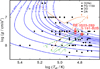 |
Fig. 1 Location of RE 0503−289 (with its error ellipse) and related objects (Hügelmeyer et al. 2006; Kepler et al. 2016; Reindl et al. 2014b,a; Werner & Herwig 2006) in the log Teff – log g plane1. Evolutionary tracks for H-deficient (Althaus et al. 2009, full lines) and H-rich WDs (Miller Bertolami 2016, dashed lines) labeled with their respective masses in M⊙ are plotted for comparison. “Wind limits” of Unglaub & Bues (2000, their Figs. 6 and 13, digitized with Dexter2) are shown. The lines indicate for H-deficient stars A: so-called PG 1159 wind limit calculated with Ṁ = 1.29 × 10⁻¹⁵L1.86; B and C: photospheric carbon content is reduced by factors of 0.5 and 0.1, respectively; D: no PG 1159 star is known to the right of this line, and for H-rich stars E: wind limit; and F: He/H = 10−3 (by number). |
2 Observations
For our spectral analysis, we used UV spectra obtained with the Far Ultraviolet Spectroscopic Explorer (FUSE, 910 Å < λ < 1190 Å, resolving power R ≈ 20 000) and the Hubble Space Telescope/Space Telescope Imaging Spectrograph (HST/STIS, 1144 Å < λ < 1709 Å with R = 2.3 × 10⁵ for G191−B2B and R ≈ 45 800 for RE 0503−289). All spectra are described in detail in Rauch et al. (2013) and Hoyer et al. (2017).
The observed spectra shown here (FUSE for λ ≤ 1188 Å, STIS otherwise) were shifted to rest wavelengths, using vrad = 24.56 km s−1 for G191−B2B (Lemoine et al. 2002)and 25.8 km s−1 for RE 0503−289 (Hoyer et al. 2017). To compare them with our synthetic spectra, they were convolved with Gaussians to simulate the respective instrument resolving power.
3 Model atmospheres and atomic data
For the precise spectral analysis of hot stars, model atmospheres that consider deviations from the local thermodynamical equilibrium (LTE) are mandatory. The Tübingen non-local thermodynamic equilibrium (NLTE) model-atmosphere package (TMAP, Werner et al. 2012b) can calculate such models that it assumes radiative and hydrostatic equilibrium and plane-parallel geometry. The Tübingen Model Atom Database (TMAD, Rauch & Deetjen 2003) provides the model atoms for elements with atomic number below 20. TMAD has been constructed as part of the Tübingen contribution to the German Astrophysical Virtual Observatory (GAVO).
The ionization stages of Cu IV–VII and In IV–VI were represented in the model atoms using so-called super levels and super lines. These were calculated via a statistical approach by our Iron Opacity and Interface (IrOnIc, Rauch & Deetjen 2003; Müller-Ringat 2013). To enable IrOnIc to read our new Cu and In data, we transferred it into Kurucz-formatted files (cf. Rauch et al. 2015b). The statistics of our Cu and In model atoms are listed in Table 1.
Our models consider opacities of He, C, N, O, Al, Si, P, S, Ca, Sc, Ti, V, Cr, Mn, Fe, Co, Ni, Cu, Zn, Ga,Ge, As, Se, Kr Sr, Zr, Mo, Sn, In, Te, I, Xe, and Ba. Details about the models are given in Rauch et al. (2016a). Cu V-VI and In VI are the dominant ionization stages in the line-forming region (− 4≲ log m≲0.5) of the photosphere of RE 0503−289 (Fig. 2).
The calculation of the Cu and In absorption cross sections is performed according to Rauch & Deetjen (2003). For the collisional bound-bound transitions we use the van Regemorter formula (van Regemorter 1962) for known f-values and an approximate formula for unknown f-values. The quadratic Stark effect is considered for radiative bound–bound transitions by an approximate formula given by (Cowley 1970, 1971). The Seaton (1962) formula is employed to calculate collisional and radiative bound-free cross sections with a hydrogen-like threshold value.
For Cu and In (and all other elements), level dissolution (pressure ionization) is considered following Hummer & Mihalas (1988) and Hubeny et al. (1994).
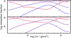 |
Fig. 2 Ionization fractions of Cu (top panel) and In (bottom) in our RE 0503−289 model. m is the column mass, measured from the outer boundary of our model atmospheres. |
Available atomic data of Cu IV–VII ions
The main source of atomic data related to the Cu IV–VII spectra is the paper published by Sugar & Musgrove (1990) in which the available experimental energy levels of the copper atom, in all stages of ionization, have been compiled together with ionization energies, either experimental or theoretical, experimental Landé g-factors, and leading components of calculated eigenvectors. This compilation is still being used as the standard reference database for the copper ions of interest at the National Institute of Standards and Technology (NIST, Kramida et al. 2019). More precisely, in Sugar and Musgrove and NIST compilations for Cu IV, experimental values are reported for 187 levels of the 3d8, 3d7 4s, 3d7 5s, 3d7 4d, and 3d6 4s2 even-parity configurations and 110 levels of the 3d74p odd-parity configuration. These data are based on earlier analyses by Schröder & van Kleef (1970), Meinders (1976), and Meinders & Uijlings (1980) who observed the copper spectrum using a sliding spark light source. In the case of Cu V, the first work was reported by van Kleef et al. (1975) who found a few energy levels in 3d7 and 3d6 4p configurations. This work was completed by van Kleef et al. (1976) who identified many 3d7 –3d64p and 3d6 4s–3d64p lines, allowing them to classify all the levels of the 3d7 configuration, as well as 53 of the 63 levels of 3d64s and 175 of the 180 levels of 3d64p. The initial line identification in the Cu VI spectrum was performed by Poppe et al. (1974) which was considerably extended a few years later by Raassen & Van Kleef (1981), who used new exposures of a sliding spark discharge to analyze the 3d6 – 3d5 4p and 3d5 4s – 3d5 4p transition arrays. This analysis led to the identification of all levels in the 3d6 configuration, except the highest 1S0, as well as 208 of the 214 levels in 3d54p and 13 of the 74 levels in 3d54s. Finally, the analysis of the Cu VII spectrum by van het Hof et al. (1990) appeared too late to be included in the compilation of Sugar & Musgrove (1990). They determined all 37 levels of the 3d5 ground configuration and 129 of the 180 possible levels of the 3d44p configuration. With regard to the radiative parameters, very few studies have focused on the determination of electric dipole transition rates in Cu IV–VII ions so far. To our knowledge, the only available data were recently obtained by Aggarwal et al. (2016) who used the quasi-relativistic approach (QR) with a very large configuration interaction (CI) expansion to compute oscillator strengths and transition probabilities in Cu VI.
Oscillator strength calculations for the Cu IV–VII ions
The method adopted in our work to model the atomic structures and compute the radiative parameters in the Cu IV–VII ions was the pseudo-relativistic Hartree-Fock (HFR) approach originally introduced by Cowan (1981) and modified to take core-polarization effects into account, giving rise to the so-called HFR+CPOL method (see, e.g., Quinet et al. 1999, 2002; Quinet 2017).
For Cu IV, configuration interaction was considered among the configurations 3d8, 3d7 4s, 3d7 5s, 3d7 4d, 3d7 5d, 3d6 4s2, 3d6 4p2, 3d6 4d2, 3d6 4s5s, and 3d6 4s4d for the even parity, and 3d74p, 3d7 5p, 3d7 4f, 3d7 5f, 3d6 4s4p, 3d6 4s5p, 3d6 4s4f, and 3d6 4p4d for the odd parity. The core-polarization parameters were the dipole polarizability of a Cu VI ionic core, as reported by Fraga et al. (1976), i.e., αd = 0.67 a.u, and the cut-off radius, rc = 0.80 a.u., corresponding to the HFR mean value ⟨r⟩ of the outermost core orbital (3d). Using the experimental energy levels compiled at NIST (Kramida et al. 2019), some radial integrals (average energy, Slater, spin-orbit, and effective interaction parameters) of 3d8, 3d7 4s, 3d7 5s, 3d7 4d, 3d6 4s2, and 3d74p configurations were optimized by a well-established least-squares fitting procedure in which the mean deviations were found to be equal to 206 cm−1 for the even parity and 183 cm−1 for the odd parity. It is worth noting that when performing the fit we found that the experimental energy level at 306 941.8 cm−1 was incorrectly classified as J = 1 in the NIST tables, while according to our calculations this level should be designated as J = 2.
For Cu V, the configurations included in the HFR model were 3d7, 3d6 4s, 3d6 5s, 3d6 4d, 3d5 4s2, 3d5 4p2, 3d5 4d2, and 3d54s4d for the even parity, and 3d64p, 3d6 5p, 3d6 4f, 3d5 4s4p, 3d5 4s5p, and 3d5 4s4f for the odd parity. In this ion the semi-empirical process was carried out to optimize the radial integrals corresponding to 3d7, 3d6 4s, and 3d6 4p configurations using the experimental levels reported in the NIST database (Kramida et al. 2019). The mean deviations between calculated and experimental energy levels were 325 cm−1 and 259 cm−1 for even and odd parities, respectively. Core-polarization effects were estimated using a dipole polarizability and a cut-off radius corresponding to a Cu VII ionic core, i.e., αd = 0.47 a.u (Fraga et al. 1976), and rc = 0.75 a.u.
In the case of Cu VI, the configuration interaction was considered among the following configurations: 3d6, 3d5 4s, 3d5 5s, 3d5 4d, 3d5 5d, 3d4 4s2, 3d4 4p2, 3d4 4d2, 3d4 4s4d, 3d4 4s5d (even parity) and 3d54p, 3d5 5p, 3d5 4f, 3d4 4s4p, 3d4 4s5p, 3d4 4s4f (odd parity). The core-polarization parameters were those corresponding to a Cu VIII ionic core, i.e., αd = 0.40 a.u (Fraga et al. 1976), and rc = 0.72 a.u The radial parameters of the 3d6, 3d5 4s, and 3d5 4p configurations were optimized to minimize the differences between the computed Hamiltonian eigenvalues and the experimental energy levels listed at NIST (Kramida et al. 2019) giving rise to mean deviations of 442 cm−1 (even parity) and 429 cm−1 (odd parity).
Finally, for Cu VII, ten even- and eight odd-parity configurations were included in the HFR model to compute the radiative parameters, i.e., 3d5, 3d4 4s, 3d4 5s, 3d4 4d, 3d4 5d, 3d3 4s2, 3d3 4p2, 3d3 4d2, 3d3 4s5s, 3d3 4s4d, and 3d44p, 3d4 5p, 3d4 4f, 3d4 5f, 3d3 4s4p, 3d3 4s5p, 3d3 4s4f, and 3d3 4p4d, respectively. An ionic core of the type Cu IX was considered to estimate the core-polarization effects with the parameters αd = 0.34 a.u (Fraga et al. 1976) and rc = 0.70 a.u The semi-empirical optimization process was carried out to adjust the radial parameters in 3d5 and 3d4 4p with the experimental energy levels taken from van het Hof et al. (1990) leading to average energy deviations of 78 cm−1 and 365 cm−1 for even and odd parities, respectively.
The parameters that we had adopted for our computations are given in Tables A.5–A.8 and a comparison of calculated and experimental energies is shown in Tables A.9–A.12 for Cu IV–VII, respectively. In Tables A.13–A.16 (provided via the registered GAVO Tübingen Oscillator Strengths Service TOSS), we give the newly computed weighted oscillator strengths (log gf) and transition probabilities(gA, in s−1) together with the experimental values (in cm−1) of the lower and upper energy levels and the corresponding Ritz wavelengths (in Å). In the final column of each table we also give the cancellation factor (CF), as defined by Cowan (1981).
Let us remind that very low values of the CF (typically <0.05) indicate strong cancellation effects in the calculation of line strengths. In these cases, the corresponding log gf and gA values could be very inaccurate and therefore need to be considered with some care. As mentioned above, no radiative rates were previously published for the copper ions considered in our work except Cu VI, for which theoretical oscillator strengths were recently reported by Aggarwal et al. (2016), who used the quasi-relativistic approach (QR) with a very large configuration interaction expansion. When comparing these latter results with ours, we found an overall good agreement, in particular for the strongest lines with log gf > −1, for which the mean deviation between the two sets of data was found to be about 20%, with a general tendency such that our log gf values appear systematically slightly higher than those of Aggarwal et al. (2016).
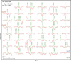 |
Fig. 3 Prominent Cu lines in the observation (gray line) of RE 0503−289, labeled with their wavelengths from Tables A.13, A.14, and A.15. Cu VI λλ 1060.890, 1100.307Å, and Cu IV λ 1410.531Å are indicated with an additional ion label, all other lines stem from Cu V. For the identification of other lines that are visible in the spectrum, please visit http://astro.uni-tuebingen.de/~TVIS/objects/RE0503-289, our Tübingen VISualization Tool (TVIS). The thick red spectrum is calculated from our best model with a Cu mass fraction of 9.3 × 10⁻⁵. The dashed green line shows a synthetic spectrum calculated without Cu. The vertical bar indicates 10% of the continuum flux. |
4 Results and conclusions
We calculated oscillator strengths of Cu IV–VII and compiled oscillator strengths of In IV (Varshney & Tauheed 2013; Ryabtsev & Kononov 2016), In V (Varshney & Tauheed 2016; Ryabtsev 2018), and In VI (Kononov et al. 2017; Ryabtsev et al. 2018) from the literature. These elements were included in our model-atmosphere calculations.
To unambiguously identify lines of one individual species, we calculated two spectra for each star (RE 0503−289 and G191−B2B), one with all opacities of that element included and one with its line opacities switched off artificially (cf. Figs. 3–5). This enables us to identify Cu and In lines, even if they are blended with other lines (cf. Tables A.1–A.3) or if they reduce the flux without exhibiting a complete line profile.
RE0503–289
We identified 54 Cu lines (1 Cu IV, 51 Cu V, and 2 Cu VI; Fig. 3, Table A.1) and 5 In V lines (Fig. 4, Table A.2). From a detailed line-profile comparison of our model (Teff = 70 000 K and log g = 7.5) with the UV observations, we found the best simultaneous agreement for all identified Cu and In lines at abundances of 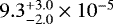 (mass fraction, 132 times solar) and
  (56 600 times solar), respectively. The Teff and log g error propagation is evaluated from two models at the error limits with highest and lowest degree of ionization, i.e., Teff = 72 000 K and log g = 7.4) and Teff = 68 000 K and log g = 7.6), respectively. We found that this abundance error is smaller than 0.1 dex. Finally, we adopted the above Cu and In mass fractions with uncertainties of 0.2 dex.
 |
Fig. 4 Same as Fig. 3, but for In. Lines are labeled with their wavelengths from Table A.2. The synthetic spectrum is calculated with an In mass fraction of 3.0 × 10⁻⁶. |
G191−B2B
The four strongest Cu V lines and/or blends in the synthetic spectrum are identified in the observation (Fig. 5, Table A.3). They are well reproduced by a model (Teff = 60 000 K, log g = 7.6) with a Cu mass fraction of  (nine times solar). The error estimation is performed analogously to that of RE 0503−289 (see above) and we found the same uncertainty of 0.2 dex.
No In line can be identified in the UV observation of G191−B2B. We used two of the strongest lines, namely In V λλ 1334.123, 1339.599Å, to determine an upper abundance limit of 5.3 × 10⁻⁷ (mass fraction, 1000 times solar; Fig. 6).
To summarize, the determined Cu and In abundances closely match the already known TIE abundance patterns in G191−B2B and RE 0503−289 (Fig. 7), which isthe result of effective radiative levitation (Rauch et al. 2016b). The TIE enrichment is much stronger in RE 0503−289 compared to that in G191−B2B due to the lower Teff of the latter (Fig. 1, Teff = 60 000 ± 2000 K and log g = 7.6 ± 0.05, Rauch et al. 2013). The relative TIE abundances in RE 0503−289, however, obviously resemble the relative solar abundance ratios (Fig. 7, cf. 29 ≤ Z ≤ 36 and 49 ≤ Z ≤ 54), i.e., higher abundances for species with even Z compared tothose with odd Z (Oddo-Harkins rule, Oddo 1914; Harkins 1917).
Surface abundance patterns that are the result of diffusion (cf. Fig. 7) and exhibit strong TIE enrichment are also found recently in He-sdOs, e.g., LS IV − 14°116 (Naslim et al. 2011), in Feige 46 (Latour et al. 2019), in HD 127493 and HZ 44, (Dorsch et al. 2019), and in the DAO-type star BD − 22°3467 (Löbling et al. 2019). However, Hoyer et al. (2017) and Rauch et al. (2019) have already mentioned that strong radiative levitation of trans-iron TIEs wipes out all information about their AGB abundances, and thus previous stellar evolution. This is general for all species in all stars with a diffusion impact on their surface abundances.
Among the WDs, RE 0503−289 exhibits lines from an unrivaled number of TIEs: 18 species (http://astro.uni-tuebingen.de/~TVIS/objects/RE0503-289). Many more lines in the UV spectral region remain unidentified. Calculations of transition probabilities of other TIEs are necessary to make further progress.
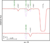 |
Fig. 6 STIS observation of G191−B2B (gray) compared with synthetic line profiles of In V λ 1334.123 Å and In V λ 1339.599 Å calculated with four In abundances: without (thin blue line), with 1000 times (thick red), 10 000 times (short-dashed violet), and 100 000 times solar abundance (long-dashed green). |
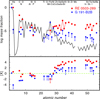 |
Fig. 7 Solar abundances (Asplund et al. 2009; Scott et al. 2015b,a; Grevesse et al. 2015, thick black line) compared with the determined photospheric abundances of G191−B2B (blue circles, Rauch et al. 2013, and this work) and RE 0503−289 (red squares, Dreizler & Werner 1996; Rauch et al. 2012, 2014a,b, 2015b, 2016b,a, 2017a,b, and this work). The uncertainties of the abundances are about 0.2 dex in general. Arrows indicate upper limits. Top panel: abundances given as logarithmic mass fractions. Determined TIE abundances of subsequent species are combined with lines. Bottom panel: abundance ratios to respective solar values, [X] denotes log (fraction / solar fraction) of species X. The dashed green line indicates solar abundances. |
Acknowledgements
The GAVO project had been supported by the Federal Ministry of Education and Research (BMBF) at Tübingen (05 AC 6 VTB, 05 AC 11 VTB) and is funded at Heidelberg (05 A 17 VH2). Financial support from the Belgian FRS-FNRS is also acknowledged. PQ is research director of this organization. Some of the data presented in this paper were obtained from the Mikulski Archive for Space Telescopes (MAST). STScI is operated by the Association of Universities for Research in Astronomy, Inc., under NASA contract NAS5-26555. Support for MAST for non-HST data is provided by the NASA Office of Space Science via grant NNX09AF08G and by other grants and contracts. The TIRO (http://astro.uni-tuebingen.de/~TIRO), TMAD (http://astro.uni-tuebingen.de/~TMAD), TOSS (http://astro.uni-tuebingen.de/~TOSS), and TVIS (http://astro.uni-tuebingen.de/~TVIS) tools and services were constructed as part of the Tübingen project (https://uni-tuebingen.de/de/122430) of the German Astrophysical Virtual Observatory (GAVO, http://www.g-vo.org). This research has made use of NASA’s Astrophysics Data System and the SIMBAD database, operated at CDS, Strasbourg, France.
Appendix A Additional tables
Identified Cu IV–VI lines in the UV spectrum of RE 0503−289.
Ions with recently calculated oscillator strengths.
Radial parameters (in cm−1) adopted for the calculations in Cu IV.
Radial parameters (in cm−1) adopted for the calculations in Cu V.
Radial parameters (in cm−1) adopted for the calculations in Cu VI.
Radial parameters (in cm−1) adopted for the calculations in Cu VII.
Comparison between available experimental and calculated energy levels in Cu IV.
Comparison between available experimental and calculated energy levels in Cu V.
Comparison between available experimental and calculated energy levels in Cu VI.
Comparison between available experimental and calculated energy levels in Cu VII.
Calculated HFR oscillator strengths (log gifik) and transition probabilities (gkAki) in Cu IV.
Calculated HFR oscillator strengths (log gifik) and transition probabilities (gkAki) in Cu V.
Calculated HFR oscillator strengths (log gifik) and transition probabilities (gkAki) in Cu VI.
Calculated HFR oscillator strengths (log gifik) and transition probabilities (gkAki) in Cu VII.
References
- Aggarwal, K. M., Bogdanovich, P., Keenan, F. P., & Kisielius, R. 2016, At. Data Nucl. Data Tables, 111, 280 [NASA ADS] [CrossRef] [Google Scholar]
- Althaus, L. G., Panei, J. A., Miller Bertolami, M. M., et al. 2009, ApJ, 704, 1605 [NASA ADS] [CrossRef] [Google Scholar]
- Asplund, M., Grevesse, N., Sauval, A. J., & Scott, P. 2009, ARA&A, 47, 481 [NASA ADS] [CrossRef] [Google Scholar]
- Cowan, R. D. 1981, The Theory of Atomic Structure and Spectra (Berkeley, CA: University of California Press) [Google Scholar]
- Cowley, C. R. 1970, The Theory of Stellar Spectra (New York: Gordon & Breach) [Google Scholar]
- Cowley, C. R. 1971, The Observatory, 91, 139 [NASA ADS] [Google Scholar]
- Dorsch, M., Latour, M., & Heber, U. 2019, A&A, 630, A130 [NASA ADS] [CrossRef] [EDP Sciences] [Google Scholar]
- Dreizler, S., & Werner, K. 1996, A&A, 314, 217 [NASA ADS] [Google Scholar]
- Fraga, S., Karwowski, J., & Saxena, K. M. S. 1976, Handbook of Atomic Data (Amsterdam: Elsevier) [Google Scholar]
- Grevesse, N., Scott, P., Asplund, M., & Sauval, A. J. 2015, A&A, 573, A27 [NASA ADS] [CrossRef] [EDP Sciences] [Google Scholar]
- Harkins, W. D. 1917, J. Am. Chem. Soc., 39, 856 [CrossRef] [Google Scholar]
- Hoyer, D., Rauch, T., Werner, K., Kruk, J. W., & Quinet, P. 2017, A&A, 598, A135 [NASA ADS] [CrossRef] [EDP Sciences] [Google Scholar]
- Hubeny, I., Hummer, D. G., & Lanz, T. 1994, A&A, 282, 151 [NASA ADS] [Google Scholar]
- Hügelmeyer, S. D., Dreizler, S., Homeier, D., et al. 2006, A&A, 454, 617 [NASA ADS] [CrossRef] [EDP Sciences] [Google Scholar]
- Hummer, D. G., & Mihalas, D. 1988, ApJ, 331, 794 [NASA ADS] [CrossRef] [Google Scholar]
- Kepler, S. O., Pelisoli, I., Koester, D., et al. 2016, MNRAS, 455, 3413 [NASA ADS] [CrossRef] [Google Scholar]
- Kononov, E. Y., Kildiyarova, R. R., Ryabtsev, A. N., et al. 2017, Euro. Phys. J. Web Conf., 132, 03023 [CrossRef] [Google Scholar]
- Kramida, A., Ralchenko, Y., Reader, J., & NIST ASD Team 2019, in NIST Atomic Spectra Database (version 5.7.1), [online]. available: https://physics.nist.gov/asd [Wed Mar 18 2020]. National Institute of Standards and Technology, Gaithersburg, MD. http://doi.org/10.18434/T4W30F [Google Scholar]
- Latour, M., Dorsch, M., & Heber, U. 2019, A&A, 629, A148 [NASA ADS] [CrossRef] [EDP Sciences] [Google Scholar]
- Lemoine, M., Vidal-Madjar, A., Hébrard, G., et al. 2002, ApJS, 140, 67 [NASA ADS] [CrossRef] [Google Scholar]
- Löbling, L., Maney, M. A., Rauch, T., et al. 2019, MNRAS, 492, 528 [NASA ADS] [CrossRef] [Google Scholar]
- McCook, G. P., & Sion, E. M. 1999a, ApJS, 121, 1 [NASA ADS] [CrossRef] [Google Scholar]
- McCook, G. P., & Sion, E. M. 1999b, VizieR Online Data Catalog: III/210 [Google Scholar]
- Meinders, E. 1976, Physica B+C, 84, 117 [NASA ADS] [CrossRef] [Google Scholar]
- Meinders, E., & Uijlings, P. 1980, Physica B+C, 100, 389 [NASA ADS] [CrossRef] [Google Scholar]
- Miller Bertolami, M. M. 2016, A&A, 588, A25 [NASA ADS] [CrossRef] [EDP Sciences] [Google Scholar]
- Müller-Ringat, E. 2013, Dissertation, University of Tübingen, Germany [Google Scholar]
- Naslim, N., Jeffery, C. S., Behara, N. T., & Hibbert, A. 2011, MNRAS, 412, 363 [NASA ADS] [CrossRef] [Google Scholar]
- Oddo, G. 1914, Z. anorganische Chemie, 87, 253 [CrossRef] [Google Scholar]
- Poppe, R., Van Kleef, T. A. M., & Raassen, A. J. J. 1974, Physica, 77, 165 [NASA ADS] [CrossRef] [Google Scholar]
- Quinet, P. 2017, Can. J. Phys., 95, 790 [NASA ADS] [CrossRef] [Google Scholar]
- Quinet, P., Palmeri, P., Biémont, É., et al. 1999, MNRAS, 307, 934 [NASA ADS] [CrossRef] [EDP Sciences] [Google Scholar]
- Quinet, P., Palmeri, P., Biémont, É., et al. 2002, J. Alloys Comp., 344, 255 [CrossRef] [Google Scholar]
- Raassen, A. J. J., & Van Kleef, T. A. M. 1981, Physica B+C, 103, 412 [NASA ADS] [CrossRef] [Google Scholar]
- Rauch, T., & Deetjen, J. L. 2003, ASP Conf. Ser., 288, 103 [NASA ADS] [Google Scholar]
- Rauch, T., Werner, K., Biémont, É., Quinet, P., & Kruk, J. W. 2012, A&A, 546, A55 [NASA ADS] [CrossRef] [EDP Sciences] [Google Scholar]
- Rauch, T., Werner, K., Bohlin, R., & Kruk, J. W. 2013, A&A, 560, A106 [NASA ADS] [CrossRef] [EDP Sciences] [Google Scholar]
- Rauch, T., Werner, K., Quinet, P., & Kruk, J. W. 2014a, A&A, 564, A41 [NASA ADS] [CrossRef] [EDP Sciences] [Google Scholar]
- Rauch, T., Werner, K., Quinet, P., & Kruk, J. W. 2014b, A&A, 566, A10 [NASA ADS] [CrossRef] [EDP Sciences] [Google Scholar]
- Rauch, T., Hoyer, D., Quinet, P., Gallardo, M., & Raineri, M. 2015a, A&A, 577, A88 [NASA ADS] [CrossRef] [EDP Sciences] [Google Scholar]
- Rauch, T., Werner, K., Quinet, P., & Kruk, J. W. 2015b, A&A, 577, A6 [NASA ADS] [CrossRef] [EDP Sciences] [Google Scholar]
- Rauch, T., Quinet, P., Hoyer, D., et al. 2016a, A&A, 590, A128 [NASA ADS] [CrossRef] [EDP Sciences] [Google Scholar]
- Rauch, T., Quinet, P., Hoyer, D., et al. 2016b, A&A, 587, A39 [NASA ADS] [CrossRef] [EDP Sciences] [Google Scholar]
- Rauch, T., Gamrath, S., Quinet, P., et al. 2017a, A&A, 599, A142 [NASA ADS] [CrossRef] [EDP Sciences] [Google Scholar]
- Rauch, T., Quinet, P., Knörzer, M., et al. 2017b, A&A, 606, A105 [NASA ADS] [CrossRef] [EDP Sciences] [Google Scholar]
- Rauch, T., Gamrath, S., Quinet, P., et al. 2019, ASP Conf. Ser., 519, 175 [NASA ADS] [Google Scholar]
- Reindl, N., Rauch, T., Werner, K., et al. 2014a, A&A, 572, A117 [NASA ADS] [CrossRef] [EDP Sciences] [Google Scholar]
- Reindl, N., Rauch, T., Werner, K., Kruk, J. W., & Todt, H. 2014b, A&A, 566, A116 [NASA ADS] [CrossRef] [EDP Sciences] [Google Scholar]
- Ryabtsev, A. N. 2018, J. Quant. Spectr. Rad. Transf., 220, 106 [NASA ADS] [CrossRef] [Google Scholar]
- Ryabtsev, A. N., & Kononov, E. Y. 2016, J. Quant. Spectr. Rad. Transf., 168, 89 [NASA ADS] [CrossRef] [Google Scholar]
- Ryabtsev, A. N., Tauheed, A., Swapnil, Kildiyarova, R. R., & Kononov, E. Y. 2018, J. Quant. Spectr. Rad. Transf., 212, 50 [NASA ADS] [CrossRef] [Google Scholar]
- Schröder, J. F., & van Kleef, T. A. M. 1970, Physica, 49, 388 [NASA ADS] [CrossRef] [Google Scholar]
- Scott, P., Asplund, M., Grevesse, N., Bergemann, M., & Sauval, A. J. 2015a, A&A, 573, A26 [NASA ADS] [CrossRef] [EDP Sciences] [Google Scholar]
- Scott, P., Grevesse, N., Asplund, M., et al. 2015b, A&A, 573, A25 [NASA ADS] [CrossRef] [EDP Sciences] [Google Scholar]
- Seaton, M. J. 1962, Atomic and Molecular Processes, ed. D. R. Bates (New York: Academic Press), 375 [Google Scholar]
- Sugar, J., & Musgrove, A. 1990, J. Phys. Chem. Ref. Data, 19, 527 [NASA ADS] [CrossRef] [Google Scholar]
- Unglaub, K., & Bues, I. 2000, A&A, 359, 1042 [NASA ADS] [Google Scholar]
- van Regemorter, H. 1962, ApJ, 136, 906 [NASA ADS] [CrossRef] [Google Scholar]
- van het Hof, G. J., Raassen, A. J. J., Uylings, P. H. M., et al. 1990, Phys. Scr., 41, 240 [NASA ADS] [CrossRef] [Google Scholar]
- van Kleef, T. A. M., Joshi, Y. N., & Benschop, H. 1975, Can. J. Phys., 53, 230 [NASA ADS] [CrossRef] [Google Scholar]
- van Kleef, T. A. M., Raasen, A. J. J., & Joshi, Y. N. 1976, Physica B+C, 84, 401 [NASA ADS] [CrossRef] [Google Scholar]
- Varshney, S., & Tauheed, A. 2013, J. Quant. Spectr. Rad. Transf., 129, 31 [CrossRef] [Google Scholar]
- Varshney, S., & Tauheed, A. 2016, J. Quant. Spectr. Rad. Transf., 168, 102 [NASA ADS] [CrossRef] [Google Scholar]
- Werner, K., & Herwig, F. 2006, PASP, 118, 183 [NASA ADS] [CrossRef] [Google Scholar]
- Werner, K., Rauch, T., Ringat, E., & Kruk, J. W. 2012a, ApJ, 753, L7 [NASA ADS] [CrossRef] [Google Scholar]
- Werner, K., Dreizler, S., & Rauch, T. 2012b, Astrophysics Source Code Library [record ascl:1212.015] [Google Scholar]
cf. http://www.astro.physik.uni-potsdam.de/~nreindl/He.html for stellar parameters.
All Tables
Comparison between available experimental and calculated energy levels in Cu IV.
Comparison between available experimental and calculated energy levels in Cu V.
Comparison between available experimental and calculated energy levels in Cu VI.
Comparison between available experimental and calculated energy levels in Cu VII.
Calculated HFR oscillator strengths (log gifik) and transition probabilities (gkAki) in Cu IV.
Calculated HFR oscillator strengths (log gifik) and transition probabilities (gkAki) in Cu V.
Calculated HFR oscillator strengths (log gifik) and transition probabilities (gkAki) in Cu VI.
Calculated HFR oscillator strengths (log gifik) and transition probabilities (gkAki) in Cu VII.
All Figures
|
Fig. 1 Location of RE 0503−289 (with its error ellipse) and related objects (Hügelmeyer et al. 2006; Kepler et al. 2016; Reindl et al. 2014b,a; Werner & Herwig 2006) in the log Teff – log g plane1. Evolutionary tracks for H-deficient (Althaus et al. 2009, full lines) and H-rich WDs (Miller Bertolami 2016, dashed lines) labeled with their respective masses in M⊙ are plotted for comparison. “Wind limits” of Unglaub & Bues (2000, their Figs. 6 and 13, digitized with Dexter2) are shown. The lines indicate for H-deficient stars A: so-called PG 1159 wind limit calculated with Ṁ = 1.29 × 10⁻¹⁵L1.86; B and C: photospheric carbon content is reduced by factors of 0.5 and 0.1, respectively; D: no PG 1159 star is known to the right of this line, and for H-rich stars E: wind limit; and F: He/H = 10−3 (by number). |
| In the text | |
|
Fig. 2 Ionization fractions of Cu (top panel) and In (bottom) in our RE 0503−289 model. m is the column mass, measured from the outer boundary of our model atmospheres. |
| In the text | |
|
Fig. 3 Prominent Cu lines in the observation (gray line) of RE 0503−289, labeled with their wavelengths from Tables A.13, A.14, and A.15. Cu VI λλ 1060.890, 1100.307Å, and Cu IV λ 1410.531Å are indicated with an additional ion label, all other lines stem from Cu V. For the identification of other lines that are visible in the spectrum, please visit http://astro.uni-tuebingen.de/~TVIS/objects/RE0503-289, our Tübingen VISualization Tool (TVIS). The thick red spectrum is calculated from our best model with a Cu mass fraction of 9.3 × 10⁻⁵. The dashed green line shows a synthetic spectrum calculated without Cu. The vertical bar indicates 10% of the continuum flux. |
| In the text | |
|
Fig. 4 Same as Fig. 3, but for In. Lines are labeled with their wavelengths from Table A.2. The synthetic spectrum is calculated with an In mass fraction of 3.0 × 10⁻⁶. |
| In the text | |
 |
Fig. 5 Same as Fig. 3, but for G191−B2B. |
| In the text | |
|
Fig. 6 STIS observation of G191−B2B (gray) compared with synthetic line profiles of In V λ 1334.123 Å and In V λ 1339.599 Å calculated with four In abundances: without (thin blue line), with 1000 times (thick red), 10 000 times (short-dashed violet), and 100 000 times solar abundance (long-dashed green). |
| In the text | |
|
Fig. 7 Solar abundances (Asplund et al. 2009; Scott et al. 2015b,a; Grevesse et al. 2015, thick black line) compared with the determined photospheric abundances of G191−B2B (blue circles, Rauch et al. 2013, and this work) and RE 0503−289 (red squares, Dreizler & Werner 1996; Rauch et al. 2012, 2014a,b, 2015b, 2016b,a, 2017a,b, and this work). The uncertainties of the abundances are about 0.2 dex in general. Arrows indicate upper limits. Top panel: abundances given as logarithmic mass fractions. Determined TIE abundances of subsequent species are combined with lines. Bottom panel: abundance ratios to respective solar values, [X] denotes log (fraction / solar fraction) of species X. The dashed green line indicates solar abundances. |
| In the text | |
Current usage metrics show cumulative count of Article Views (full-text article views including HTML views, PDF and ePub downloads, according to the available data) and Abstracts Views on Vision4Press platform.
Data correspond to usage on the plateform after 2015. The current usage metrics is available 48-96 hours after online publication and is updated daily on week days.
Initial download of the metrics may take a while.