| Issue |
A&A
Volume 637, May 2020
|
|
|---|---|---|
| Article Number | A86 | |
| Number of page(s) | 27 | |
| Section | Extragalactic astronomy | |
| DOI | https://doi.org/10.1051/0004-6361/201834603 | |
| Published online | 21 May 2020 | |
Study of the variable broadband emission of Markarian 501 during the most extreme Swift X-ray activity
1
Inst. de Astrofísica de Canarias, 38200 La Laguna, Spain
2
Universidad de La Laguna, Dpto. Astrofísica, 38206 La Laguna, Tenerife, Spain
3
Università di Udine and INFN Trieste, 33100 Udine, Italy
4
National Institute for Astrophysics (INAF), 00136 Rome, Italy
5
Croatian MAGIC Consortium: University of Rijeka, 51000 Rijeka; University of Split – FESB, 21000 Split; University of Zagreb – FER, 10000 Zagreb; University of Osijek, 31000 Osijek; Rudjer Boskovic Institute, 10000 Zagreb, Croatia
6
Saha Institute of Nuclear Physics, HBNI, 1/AF Bidhannagar, Salt Lake, Sector-1, Kolkata 700064, India
7
Centro Brasileiro de Pesquisas Físicas (CBPF), 22290-180 URCA, Rio de Janeiro, RJ, Brasil
8
Unidad de Partículas y Cosmología (UPARCOS), Universidad Complutense, 28040 Madrid, Spain
9
University of Łódź, Department of Astrophysics, 90236 Łódź, Poland
10
Deutsches Elektronen-Synchrotron (DESY), 15738 Zeuthen, Germany
11
Istituto Nazionale Fisica Nucleare (INFN), 00044 Frascati, Roma, Italy
12
Max-Planck-Institut für Physik, 80805 München, Germany
13
Institut de Física d’Altes Energies (IFAE), The Barcelona Institute of Science and Technology (BIST), 08193 Bellaterra, Barcelona, Spain
14
Università di Siena and INFN Pisa, 53100 Siena, Italy
15
Università di Padova and INFN, 35131 Padova, Italy
16
Università di Pisa and INFN Pisa, 56126 Pisa, Italy
17
Finnish MAGIC Consortium: Finnish Centre of Astronomy with ESO (FINCA), University of Turku, 20014 Turku, Finland; Astronomy Research Unit, University of Oulu, 90014 Oulu, Finland
18
Technische Universität Dortmund, 44221 Dortmund, Germany
19
Departament de Física and CERES-IEEC, Universitat Autònoma de Barcelona, 08193 Bellaterra, Spain
20
Universitat de Barcelona, ICCUB, IEEC-UB, 08028 Barcelona, Spain
21
ICRANet-Armenia at NAS RA, 0019 Yerevan, Armenia
22
Japanese MAGIC Consortium: ICRR, The University of Tokyo 277-8582 Chiba, Japan; Department of Physics, Kyoto University, 606-8502 Kyoto, Japan; Tokai University, 259-1292 Kanagawa, Japan; RIKEN, 351-0198 Saitama, Japan
23
Inst. for Nucl. Research and Nucl. Energy, Bulgarian Academy of Sciences, 1784 Sofia, Bulgaria
24
Humboldt University of Berlin, Institut für Physik, 12489 Berlin, Germany
25
Dipartimento di Fisica, Università di Trieste, 34127 Trieste, Italy
26
Port d’Informació Científica (PIC), 08193 Bellaterra, Barcelona, Spain
27
INAF-Trieste and Dept. of Physics & Astronomy, University of Bologna, Bologna, Italy
28
ETH Zurich, 8093 Zurich, Switzerland
29
ISDC – Department of Astronomy, University of Geneva, 16, 1290 Versoix, Switzerland
30
Universität Würzburg, 97074 Würzburg, Germany
31
RWTH Aachen University, Aachen, Germany
32
Center for Research and Exploration in Space Science and Technology (CRESST) and NASA Goddard Space Flight Center, Greenbelt, MD 20771, USA
33
Department of Physics, University of Maryland, Baltimore County, 1000 Hilltop Circle, Baltimore, MD 21250, USA
34
Space Science Data Center – ASI, Via del Politecnico, s.n.c., 00133 Roma, Italy
35
INAF–Osservatorio Astronomico di Roma, Via di Frascati 33, 00040 Monteporzio, Italy
36
Aalto University Metsähovi Radio Observatory, Metsähovintie 114, 02540 Kylmälä, Finland
37
Aalto University Department of Electronics and Nanoengineering, PO BOX 15500 00076 Espoo, Finland
Received:
7
November
2018
Accepted:
25
December
2019
Context. Markarian 501 (Mrk 501) is a very high-energy (VHE) gamma-ray blazar located at z = 0.034, which is regularly monitored by a wide range of multi-wavelength instruments, from radio to VHE gamma rays. During a period of almost two weeks in July 2014, the highest X-ray activity of Mrk 501 was observed in ∼14 years of operation of the Neil Gehrels Swift Gamma-ray Burst Observatory.
Aims. We characterize the broadband variability of Mrk 501 from radio to VHE gamma rays during the most extreme X-ray activity measured in the last 14 years, and evaluate whether it can be interpreted within theoretical scenarios widely used to explain the broadband emission from blazars.
Methods. The emission of Mrk 501 was measured at radio with Metsähovi, at optical–UV with KVA and Swift/UVOT, at X-ray with Swift/XRT and Swift/BAT, at gamma ray with Fermi-LAT, and at VHE gamma rays with the FACT and MAGIC telescopes. The multi-band variability and correlations were quantified, and the broadband spectral energy distributions (SEDs) were compared with predictions from theoretical models.
Results. The VHE emission of Mrk 501 was found to be elevated during the X-ray outburst, with a gamma-ray flux above 0.15 TeV varying from ∼0.5 to ∼2 times the Crab nebula flux. The X-ray and VHE emission both varied on timescales of 1 day and were found to be correlated. We measured a general increase in the fractional variability with energy, with the VHE variability being twice as large as the X-ray variability. The temporal evolution of the most prominent and variable segments of the SED, characterized on a day-by-day basis from 2014 July 16 to 2014 July 31, is described with a one-zone synchrotron self-Compton model with variations in the break energy of the electron energy distribution (EED), and with some adjustments in the magnetic field strength and spectral shape of the EED. These results suggest that the main flux variations during this extreme X-ray outburst are produced by the acceleration and the cooling of the high-energy electrons. A narrow feature at ∼3 TeV was observed in the VHE spectrum measured on 2014 July 19 (MJD 56857.98), which is the day with the highest X-ray flux (>0.3 keV) measured during the entire Swift mission. This feature is inconsistent with the classical analytic functions to describe the measured VHE spectra (power law, log-parabola, and log-parabola with exponential cutoff) at more than 3σ. A fit with a log-parabola plus a narrow component is preferred over the fit with a single log-parabola at more than 4σ, and a dedicated Monte Carlo simulation estimated the significance of this extra component to be larger than 3σ. Under the assumption that this VHE spectral feature is real, we show that it can be reproduced with three distinct theoretical scenarios: (a) a pileup in the EED due to stochastic acceleration; (b) a structured jet with two-SSC emitting regions, with one region dominated by an extremely narrow EED; and (c) an emission from an IC pair cascade induced by electrons accelerated in a magnetospheric vacuum gap, in addition to the SSC emission from a more conventional region along the jet of Mrk 501.
Key words: galaxies: active / BL Lacertae objects: individual: Mrk 501 / gamma rays: galaxies / X-rays: galaxies
© ESO 2020
1. Introduction
Markarian 501 (Mrk 501) is a well-known gamma-ray blazar located at z = 0.034. It was first detected at very high-energy (VHE, E > 100 GeV) gamma rays with the Whipple Observatory (Quinn et al. 1996). It is classified as a BL Lac object, whose optical spectra are dominated by the nonthermal continuum from the jet. In BL Lac objects there are no signs of a strong broad-line region (BLR) or of a dusty IR torus, and therefore, in absence of any strong external photon field interacting with the jet, they are typically modeled by synchrotron self-Compton models (SSC; see, e.g., Maraschi et al. 1992).
Mrk 501 is one of the few VHE objects that can be detected with the current generation of Imaging Air Cherenkov Telescopes (IACTs) in relatively short integration times even during their low state emission periods. This makes Mrk 501 an ideal blazar for long-term multi-wavelength (MWL) monitoring with the aim of performing detailed studies that cannot be carried out for other blazars that are fainter, located farther away, or have more complicated structures. Motivated by this goal, an extensive multi-instrument program was organized to characterize and study the temporal evolution, over many years, of the broadband emission of Mrk 501 (see, e.g., Abdo et al. 2011; Aleksić et al. 2015a; Furniss et al. 2015; Ahnen et al. 2017, 2018). This observational campaign was enhanced by the beginning of the Fermi era, providing a continuous coverage over a wide range of gamma-ray energies. Thanks to the large amount of data already investigated in the past, the extensive time and energy coverage keep bringing new clues to better understand the emission mechanisms of this blazar.
During the MWL campaign performed in July 2014, we observed a ∼two-week flaring activity in the X-ray and VHE bands. The X-ray activity was exceptionally high, yielding the largest fluxes detected with the X-ray Telescope (XRT) instrument on board the Neil Gehrels Swift Gamma-ray Burst Observatory (Gehrels et al. 2004) during its almost 14 years of operation after its launch in 2004. The X-ray activity during these two weeks appears to be similar to that observed during the large historical flare from 1997, when the BeppoSAX satellite reported a large increase in the X-ray flux of Mrk 501. During this 1997 flare, the peak of the synchrotron bump was located above 100 keV, hence indicating a shift by more than two orders of magnitude of the peak position compared to that of the typical (nonflaring) state (Pian et al. 1998; Villata & Raiteri 1999; Tavecchio et al. 2001). Within the framework of the planned multi-instrument observations, the First G-APD Cherenkov Telescope (FACT) was observing Mrk 501 daily (provided atmospheric conditions allow), but other facilities such as Metsähovi, KVA, Swift, and MAGIC were observing only once every a few days (typically once every 3–4 days). Triggered by the outstanding X-ray activity observed in the Swift data collected during the campaign, we organized multi-band observations every day, as shown in Fig. 1. These multi-instrument data allowed us to characterize with a wide energy coverage and fine temporal sampling the evolution of the broadband spectral energy distribution (SED) during this period of outstanding activity. This manuscript reports the results from these measurements together with a characterization of the variability and correlation among the various energy bands, and a physical interpretation of this remarkable behavior using theoretical leptonic scenarios that are commonly used in the literature.
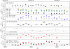 |
Fig. 1. Multi-wavelength light curve for Mrk 501 during the highest X-ray activity measured with Swift/XRT to date. The correspondence between the instruments and the measured quantities is given in the legends. The horizontal dashed lines in the VHE light curves depict the flux of the Crab nebula reported in Aleksić et al. (2016b). For BAT, the daily fluxes were computed using the spectral shape from the time interval MJD 56854.5–MJD 56872.5 (see Sect. 2.4.1). |
This paper is structured as follows. In Sect. 2 we briefly describe the instruments whose data are used, along with their data analyses. In Sect. 3 we report all the observational results, namely the multi-instrument light curves, the quantification of the variability and correlations among energy bands, and a detailed study of the X-ray and VHE gamma-ray spectra. Sections 4 and 5 characterize the broadband SED and its temporal evolution within standard leptonic scenarios, and provide a theoretical interpretation of the obtained results. Finally, Sect. 6 provides a short summary and concluding remarks. Additional details on the analysis are given in the appendix. Throughout this work we adopt the cosmological parameters H0 = 70 km s−1 Mpc−1, ΩΛ = 0.7, and ΩM = 0.3.
2. Multi-wavelength observations
Many different observatories, from radio to VHE gamma rays, participated in the MWL campaign on Mrk 501 performed between March and September 2014. The extensive dataset collected during the 2014 campaign will be reported in a future study. In this paper, we only report measurements from the ∼two-week interval in July 2014 when an extremely high X-ray activity was observed. This paper focuses mainly on the X-ray and VHE gamma-ray bands, which are the two segments of the broadband SED with the highest energy flux, and that show the highest variability (see Sect. 3). In the following sections the observations and data analyses for each instrument used in this work will be briefly described.
2.1. MAGIC
The MAGIC stereoscopic telescope system is composed of two IACTs located at the Roque de los Muchachos Observatory on La Palma, one of the Canary Islands (28.7° N, 17.9° W), at a height of 2200 m above sea level (Aleksić et al. 2016a). Each telescope has a large mirror dish 17 m in diameter. MAGIC can detect air Cherenkov showers initiated by gamma rays in the energy range from ∼50 GeV to ∼50 TeV.
This paper reports MAGIC data taken from 2014 July 16 to 2014 July 31 (MJD 56854−56869). The observations were performed within a zenith angle range from 10.0° to 41.2°. The energy threshold of the analysis, calculated as the peak of the number of events for these observation conditions and a spectral index of −2.2, is located at approximately 130 GeV. Since the data sample covers a wide range of zenith angles, the low zenith angle data allow us to characterize the spectrum at energies below the average energy threshold. The data analysis was carried out using the standard analysis package developed by the MAGIC Collaboration named MAGIC Analysis and Reconstruction Software (MARS, Zanin et al. 2013; Aleksić et al. 2016b). Mrk 501 was observed with the MAGIC telescopes for a total of 13.5 h under dark and good quality conditions. Detailed information about the data collection can be found in Table 1.
Summary of the Mrk 501 VHE observations performed with the MAGIC telescopes during the flaring activity that occurred in July 2014.
2.2. FACT
The First G-APD Cherenkov Telescope is located next to the two MAGIC telescopes. With its 9.5 m2 mirror and its camera consisting of 1440 pixels with silicon-based photosensors (G-APDs, also known as SiPM), it has been designed to perform an intense monitoring of bright TeV blazars (Anderhub et al. 2013; Biland et al. 2014). FACT has been operating since October 2011, and it has already collected more than 11 000 h of data.
This manuscript reports FACT observations of Mrk 501 from 2014 July 14 until 2014 August 5, amounting to 51.8 h, of which 47.2 h passed the quality selection based on the cosmic-ray rate described in Hildebrand et al. (2017). The FACT analysis was performed as described in Dorner et al. (2015). The excess rate was corrected for the effect of changing zenith distance and changing trigger threshold as described in Dorner et al. (2013) and Mahlke et al. (2017). The identically corrected excess rate measured from the Crab nebula during the same season was used to convert the observed excess rates into photon fluxes. The resulting light curve, with an energy threshold of about 0.83 TeV, is shown in Fig. 1. The analysis pipeline does not permit reliable spectral measurements for the observations reported here. Variability in the spectral shape of Mrk 501 would introduce an additional uncertainty in the FACT fluxes reported in Fig. 1. However, given the spectral variability measured with MAGIC (see Table A.3), this systematic error would be only ∼5%, which is much smaller than the statistical uncertainties on the VHE fluxes measured by FACT reported in Fig. 1.
2.3. Fermi-LAT
We analyzed the data collected by the Large Area Telescope (LAT) on board the Fermi Gamma-ray Space Telescope from 200 MeV to 800 GeV. The data selection was centered at the position of Mrk 501 and a circular region of 10° was chosen. The analysis used Pass 8 source class events. A first unbinned likelihood analysis was carried out for 8 months of data from 2014 April 1 to 2014 December 1 (MJD 56748−56992) in order to discard nonvariable weak sources that cannot be detected by Fermi-LAT on short timescales. In this first step, all the sources present in the 3FGL catalog (Acero et al. 2015) within 20° of Mrk 501 were included in the analysis (85 point-like sources). The sources located within 10° were left free to vary both in flux and spectral shape. On the contrary, for the sources beyond 10°, only the flux normalization was left free while the spectral shapes where fixed to their 3FGL catalog values. The analysis was performed using the Science-Tools software package version v11-07-00, the instrument response function P8R2_SOURCE_V6 and the diffuse background models gll_iem_v06 and iso_P8R2_SOURCE_V6_v061. After the first unbinned likelihood fit, the sources with test statistics (TS, Mattox et al. 1996) value of TS < 5 were removed from the model. The resulting simplified model was used to analyze the two-week period covered by the flare detected at VHE gamma rays and X-rays. The preliminary FL8Y point source list2 was checked to search for any additional source not previously included in the 3FGL catalog which might have an impact on the analysis. No new sources with TS > 25 were found within 20° from Mrk 501.
The light curve (LC) was calculated with a three-day binning because Mrk 501 is a relatively weak source for Fermi-LAT. For the LC analysis, the shape of the source spectrum was described with a power-law function, with the flux normalization as a free parameter, and the spectral index fixed to Γ = 1.78, which is the value found for the almost ∼two-week time period considered in this manuscript3. The normalizations of the diffuse background models were allowed to vary during the likelihood fit. Additionally, we also performed a spectral analysis of Fermi-LAT data for two time intervals, 4 days and 10 days, centered at the time of the observations performed daily with MAGIC. Due to the low photon statistics, it is not possible to derive constraining spectral parameters in shorter observation windows for Fermi-LAT observations of Mrk 501. Owing to the variability on one-day timescales measured at X-ray and VHE energies, the Fermi-LAT spectral points are considered an estimate of the HE spectra at the time of the X-ray and VHE observations, and used only as a guide in the theoretical modeling of the broadband SEDs.
2.4. Swift
This study reports observations performed with the three instruments on board the Neil Gehrels Swift Gamma-ray Burst Observatory (Gehrels et al. 2004); namely the Burst Alert Telescope (BAT, Markwardt et al. 2005), the X-ray Telescope (XRT, Burrows et al. 2005), and the Ultraviolet/Optical Telescope (UVOT, Roming et al. 2005).
2.4.1. BAT
We analyzed the BAT data available from Mrk 501 during the period of high activity in July 2014. We use BAT survey data in this analysis, which contain 80 energy channels and are pre-binned by the onboard software in ∼300 s (for details, see Sect. 3.3.1 in Markwardt et al. 2007). These data are processed using the standard BAT pipeline, batsurvey4. We adopted eight energy bands in our analysis from 14 to 195 keV. When computing the BAT fluxes in one-day time intervals, these eight channels had to be combined into a single energy bin because of the low signal event count. For each observation, the batsurvey pipeline produced the mask-weighted counts (i.e., background-subtracted counts) in these eight energy bands at the source location. We added up the resulting counts in each day and calculated the corresponding uncertainties through error propagation, and then used this information to create an eight energy band spectrum. As we only use the survey data when Swift was pointing at Mrk 501, the counts could be added up without adjusting for different source incident angles and partial coding fractions. We then used the BAT tool batdrmgen to generate the corresponding BAT detector response file.
The analysis was performed using two different timescales: daily analysis integrating the observations within one day centered at the MAGIC observations, and a stacked analysis over the time interval considered in this manuscript, namely MJD 56854.5–MJD 56872.5. In the stacked analysis (60.2 ks of exposure), the source is detected with a signal-to-noise ratio of 19.2 and is well described by a power-law function (χ2/d.o.f. = 2.4/6) with spectral index of 2.3 ± 0.1 and a flux of (4.1 ± 0.3) × 10−10 erg cm−2 s−1 in the 14–195 keV energy band.
The BAT flux for each day during this observation period was found by fitting the eight-bin spectra using the commonly adopted X-ray Spectral Fitting Package, Xspec5. Because the source is only detected at a relatively low significance on a daily timescale, we only allowed the flux normalization to vary in the fitting procedure. Two different spectral shapes were used: (a) the power-law function from the 18-day stacked analysis of the BAT data and (b) the spectral parameters from the XRT spectral analysis reported in Table A.1. The calculation of the flux and uncertainty range were carried out with Xspec, using the cflux command. In the spectral analysis for MJD 56862, the counts are too low and Xspec did not find any solution. Consequently, we calculated the 2σ flux upper limit based on the exposure time using Eq. (9) in Baumgartner et al. (2013), which gives an approximation of the BAT sensitivity. The results are reported in Table A.2.
2.4.2. XRT
The XRT data were taken in the framework of the planned extensive multi-instrument campaign. The high activity of Mrk 501 in the X-ray band motivated the increase in the number of observations from one pointing every ∼4 days, to one per day between MJD 56855 and MJD 56870. All observations were carried out in the Windowed Timing (WT) readout mode, with an exposure of ∼1 ks per pointing. The data were processed using the XRTDAS software package (v.3.4.0), which was developed by the ASI Science Data Center and released by HEASARC in the HEASoft package (v.6.2.2). The data were calibrated and cleaned with standard filtering criteria using the xrtpipeline task and the calibration files available from the Swift/XRT CALDB (version 20140709). For the spectral analysis, events in the energy channels between 0.3 keV and 10 keV were selected within a 20 pixel (∼46 arcsec) radius, which contains 90% of the point spread function (PSF). The background was estimated from a nearby circular region with a radius of 20 pixels. Corrections for the PSF and CCD defects were applied from response files generated using the xrtmkarf task and the cumulative exposure map. The spectra were binned to ensure a minimum of 20 counts per bin, fitted in the band 0.3–10 keV, and corrected for absorption with a neutral-hydrogen column density fixed to the Galactic 21 cm value in the direction of Mrk 501, namely 1.55 × 1020 cm−2 (Kalberla et al. 2005). The spectral results are reported in Table A.1.
2.4.3. UVOT
We also used the Swift/UVOT observations performed with the UV lenticular filters (W1, M2, and W2) that were taken within the same observations acquired by XRT. The emission from these bands is not affected by the host galaxy emission. We evaluated the photometry of the source according to the recipe in Poole et al. (2008), extracting source counts with an aperture of 5 arcsec radius and an annular background aperture with inner and outer radii of 20 arcsec and 30 arcsec. The count rates were converted to fluxes using the updated calibrations (Breeveld et al. 2011). Flux values were then corrected for mean Galactic extinction using an E(B − V) value of 0.017 (Schlafly & Finkbeiner 2011) using the UVOT filter effective wavelength and the mean Galactic interstellar extinction curve in Fitzpatrick (1999).
2.5. Optical and radio
The optical data in the R band were obtained with the KVA telescope, at the Roque de los Muchachos (La Palma, Spain). The data analysis was performed as described in Nilsson et al. (2018). The calibration was performed using the stars reported by Villata et al. (1998) and the Galactic extinction was corrected using the coefficients given in Schlafly & Finkbeiner (2011). The contribution from the host galaxy in the R band, which is about 2/3 of the measured flux, was determined using Nilsson et al. (2007), and subtracted from the values reported in Fig. 1.
The radio fluxes at 37 GHz were obtained with the 14 m Metsähovi Radio telescope at the Metsähovi Radio Observatory. Details of the observation and analysis strategies are given in Teraesranta et al. (1998).
3. Results
3.1. Multi-wavelength flux evolution and quantification of the variability
The MWL LC from radio to the VHE band is reported in Fig. 1. Only marginal variability is detected in radio, optical-UV, and low-energy gamma rays above 200 MeV observed by Fermi-LAT. On the contrary, there are large flux variations in X-rays and VHE gamma rays. In both energy bands, the flux evolution during the two-week high activity shows a two-peak structure of similar amplitude with respect to each other. Variability on one-day timescales is significantly detected, but no intra-night variability is observed in any of the energy bands studied in this work.
To quantify and compare the variability observed at different energy bands, the fractional variability (Fvar) is calculated. Following the prescription from Vaughan et al. (2003), Fvar is defined as
where ⟨Fγ⟩ denotes the average photon flux, S the standard deviation of the different flux measurements, and  represents the mean squared error of the flux measurements. The uncertainty of Fvar is calculated following the prescription in Poutanen & Zdziarski (2008), as described in Aleksić et al. (2015a), such that these uncertainties are also valid in the case when ΔFvar ∼ Fvar,
where  is calculated following Eq. (11) from Vaughan et al. (2003). This prescription to determine the multi-band variability has some caveats related to the different sensitivity and observing sampling among the various instruments used (see, e.g., Aleksić et al. 2014a, 2015b). However, it provides a relatively simple way of quantifying and comparing the flux variability in the different energy bands.
The results of the Fvar calculation for each energy band, as reported in Fig. 1, are shown in Fig. 2. The fractional variability is not defined in the case of radio and HE gamma rays observed with Fermi-LAT, as the excess variance is negative (S2 is smaller than  ). A negative excess variance implies that either there is no variability or that the instruments are not sensitive enough to detect it.
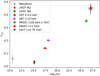 |
Fig. 2. Fractional variability Fvar as a function of frequency. |
There is a general increase in the fractional variability with increasing energy of the emission, showing the highest variability in the VHE band. At optical and UV bands the fractional variability is about 0.05, at the X-ray bands it is about 0.2, and at the VHE gamma-ray bands it is about 0.4. A comparable variability pattern in the broadband emission of Mrk 501 has been observed in most of the previous extensive campaigns (see, e.g., Aleksić et al. 2015a; Ahnen et al. 2017, 2018), indicating that it is a typical characteristic of Mrk 501, during low and high activity. In contrast, for the other classical TeV blazar, Mrk 421, a well-defined double-peak structure is observed in the plot of Fvar versus energy, where the variability in the X-ray band is comparable (and even greater) than that at VHE gamma-ray energies (see, e.g., Aleksić et al. 2015b,c; Baloković et al. 2016).
3.2. Correlation between the X-ray and VHE gamma-ray bands
This section investigates the cross-correlation between the two segments of the electromagnetic spectrum with the highest variability, namely the X-rays and the VHE gamma rays (see Fig. 2). Figure 3 shows the integral VHE gamma-ray flux from two energy bands (0.15–1 TeV and > 1 TeV) measured by MAGIC, plotted against the X-ray flux in two energy bands (0.3–2 keV and 2–10 keV) observed by Swift/XRT. The 13 X-ray and VHE fluxes depicted in this figure are taken within a maximum difference of 3 h from each other6. Given that we did not find any significant intra-night variability (neither in the Swift/XRT nor in the MAGIC and FACT data), the used X-ray and VHE data can be safely considered simultaneous. The correlation between these two bands is quantified using two methods: the Pearson correlation coefficient (and the significance of this correlation) and the discrete correlation function (DCF, Edelson & Krolik 1988). The DCF has an advantage over the Pearson correlation in that it also uses the uncertainties in the individual flux measurements, which naturally contribute to the dispersion in the flux values. The results are shown in Table 2. Despite the relatively short time interval considered in this study, and that Mrk 501 was in an elevated state at X-rays and VHE gamma-rays during the entire period, we observe a significant correlation between the X-ray and VHE gamma-ray bands. This correlation increases slightly with the increasing energy in X-rays: it is ∼3σ for the 0.3–2 keV band and ∼4σ for the 2–10 keV band. A stronger correlation with increasing X-ray energy was also reported for Mrk 501 (see Tables 1 and 4 of Ahnen et al. 2018), but in that case for a much longer time interval (three months instead of two weeks). These observations indicate that, within the one-zone SSC theoretical framework, the electrons that dominate the emission at 2–10 keV make a larger contribution to the emission at VHE gamma rays than those that dominate the emission at 0.3–2 keV (see Ahnen et al. 2018, for further details).
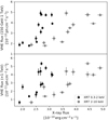 |
Fig. 3. VHE flux in two energy bands (0.15–1 TeV and > 1 TeV) as a function of the Swift/XRT flux in two energy bands (0.3–2 keV and 2–10 keV). |
Quantification of the correlation: VHE vs X-ray flux at different energy bands.
It is interesting to note that during periods of low activity the correlation between the X-ray and VHE bands has been shown to be only marginally significant or even nonexistent (see, e.g., Aleksić et al. 2015a; Ahnen et al. 2017, 2018). On the other hand, this correlation is very strong for well-sampled and long-term light curves covering periods of low activity together with periods of very high activity (see, e.g., Gliozzi et al. 2006). Naturally, our ability to detect significant correlations improves when considering accurate flux measurements and periods with large flux changes. The study reported here shows, for the first time for Mrk 501, a significant (>3σ) correlated behavior between X-rays and VHE gamma rays during a short period of time (two weeks) of persistent elevated activity. A correlation on weekly timescales was also claimed for Mrk 501 in Catanese et al. (1997) and Sambruna et al. (2000), but the significance of this correlation was not computed in either of these two previous studies. On the other hand, a significant correlation between the X-ray and the VHE gamma-ray band during a ∼two-week elevated state has also been reported for Mrk 421 (Aleksić et al. 2015c). Such a X-ray–VHE correlation is actually expected within the framework of the synchrotron self-Compton (SSC) emission scenario (see, e.g., Maraschi et al. 1992), which predicts that the X-ray and the VHE gamma-ray emission are produced by the same population of electrons and positrons. This is the most widely used theoretical scenario for describing the emission of high-peaked BL Lac-type objects such as Mrk 501, and will be also used to model the broadband SEDs of these two weeks of remarkably high X-ray activity (see Sect. 4).
3.3. X-ray and VHE gamma-ray spectral variability
Most of the X-ray spectra measured with Swift/XRT are well characterized by a power-law function (PL), as reported in Table A.1. A hint of harder-when-brighter evolution is observed in X-rays at ∼2σ and ∼4σ for soft (0.3–2 keV) and hard (2–10 keV) X-rays, respectively, as reported in Appendix B.
The VHE gamma-ray spectra from MAGIC are characterized on one-day timescales because we did not find any significant intra-night variability during the observation campaign reported in this paper, despite Mrk 501 having shown flux and spectral variability on time scales of a few minutes (Albert et al. 2007). The gamma-ray spectra are absorbed and distorted due to the interaction with the extragalactic background light (EBL) via pair production of an electron and a positron (see, e.g., Domínguez et al. 2011, and references therein). Both the observed and EBL-corrected (assuming the EBL model from Domínguez et al. 2011) VHE spectra can typically be well fitted by a simple PL function (Eq. 3), except for two or three cases out of the 15 nights which show curvature, and a log-parabola fit (LP, Eq. (4)) is preferred over a PL fit with a significance higher than 3σ (see Table A.3). The PL function is defined as
where f0 represents the normalization constant and Γ the spectral index. The LP function is given by
which uses the b parameter in addition to Eq. (3) to parameterize the spectral curvature.
The flux and spectral evolution in the VHE band, as observed by MAGIC, does not show a harder-when-brighter trend, as reported in Appendix B. During the observations taken on 2014 July 19 (MJD 56857.98), which is the day with the highest X-ray flux above 0.3 keV measured by Swift during its entire operation, a hint of a narrow spectral feature is observed. The investigation of this feature is discussed in Sect. 3.4.
3.4. Investigation of a feature in the VHE spectrum from 2014 July 19
The VHE spectrum observed by MAGIC on 2014 July 19 shows a hint of a narrow spectral feature, as depicted in the upper panel of Fig. 4. To test the significance of this feature, the goodness of the fit to the spectrum was evaluated by means of a χ2 test using different functions: a PL (see Eq. (3)), an LP (Eq. (4)), and an exponential log-parabola (ELP) defined as
where in addition to the parameters used in Eq. (4), the parameter Ec sets the exponential cutoff energy. These three spectral functions have been widely used to successfully parameterize the spectra of VHE gamma-ray sources.
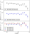 |
Fig. 4. VHE SEDs from the MAGIC telescopes during the highest X-ray flux measured with Swift/XRT. Top and middle panels: black circles represent the observed SED from 2014 July 19 (MJD 56857.98), while the blue squares denote the same spectrum corrected for EBL absorption (using the model from Domínguez et al. 2011). In both panels the dotted lines depict the best LP fits (reported in Table 3), while the dashed lines show the best fits using data up to 1.5 TeV, and extrapolated beyond that energy (from the test reported in Table C.1). Bottom panel: VHE SEDs after EBL correction during three consecutive nights around 2014 July 19 (MJD 56857.98). |
Results from the forward-folding fits with three different functions (PL, LP, and ELP) to the MAGIC VHE spectra observed and EBL-corrected (using the EBL model from Domínguez et al. 2011) from 2014 July 19 (MJD 56857.98).
The parameters and the goodness of the spectral fits for both the observed and EBL-corrected spectra are reported for the three functions (PL, LP, ELP) in Table 3. We note that the reported spectral fits were obtained with a forward-folding procedure (procedure details given in Acciari et al. 2019), where the number of degrees of freedom is related to the bins in estimated energy and not to the bins in true energy, which is what is shown in the broadband SEDs (Fig. 4). As shown in Table 3, neither the observed nor the EBL-corrected spectrum can be fitted successfully with any of the three functions. The fits to the observed VHE spectra can be rejected at significance values ranging from 3.3σ to 4.6σ, depending on the function. For the EBL-corrected spectrum, the rejection occurs at significance values from 2.9σ to 3.1σ.
A further test is performed fitting with an LP (to allow possible curvature) all the single-night spectra up to 1.5 TeV, and evaluating the model-data agreement when extending the resulting fit function to energies higher than 1.5 TeV. This approach allows us to quantify how much the spectra change at high energies with respect to the low energies, and hence investigate the potential existence of additional spectral components. This test is carried out only for the spectra with at least three spectral points beyond 1.5 TeV. The table with the results is found in Appendix C. As shown in Table C.1, the only extended fit beyond 1.5 TeV that can be rejected with a high confidence level is the one for the night of MJD 56857.98, with a significance of 5.3σ for the observed spectrum and 4.2σ for the EBL-corrected spectrum.
Motivated by the difficulty of fitting the spectrum from 2014 July 19 with the typical analytic functions used to describe the VHE spectra of blazars, we compare the goodness of the fit for an LP function with respect to an LP plus a strongly curved LP, described as an eplogpar model (EP, Tramacere et al. 2007) described in Eq. (6), using a likelihood ratio test (LRT, where  with degrees of freedom d.o.f. = d.o.f.LP–d.o.f.LP + EP).
where K is a constant, Ep represents the energy peak, and β is the curvature term. The resulting spectral fits are depicted in Fig. 5 and the fit parameter values are reported in Table 4. In order to better characterize the relatively narrow spectral feature, we increased by 25% the number of bins in estimated energy with respect to those used in the spectral fits performed on all the single-night VHE spectra reported in this manuscript (see Tables 3 and A.3). This also increased the number of bins in true energy (i.e., the number of data points in Fig. 5 is larger than that of Fig. 4). This fine energy binning used to derive the spectral fitting results for 2014 July 19, as reported in Fig. 5 and Table 4, would not work on other days with lower gamma-ray activity and/or shorter observation times, due to the lower photon statistics. The LRT shows that the LP with the additional narrow component is preferred over the single LP function at 4.5σ when using the observed spectrum and 3.9σ when using the EBL-corrected spectrum.
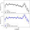 |
Fig. 5. VHE SED from 2014 July 19 (MJD 56857.98) measured with the MAGIC telescopes with an analysis that uses 25% more bins in estimated energy with respect to that shown in Fig. 4. Black circles represent the observed SED, while the blue squares denote the same spectrum corrected for EBL absorption (using the model from Domínguez et al. 2011). In both panels the dotted lines depict fits with an LP function, while the solid lines depict the fits with an LP+EP function. The parameter values resulting from the spectral fits are reported in Table 4. |
Results from the forward-folding fits with an LP and an LP+EP to the MAGIC VHE spectra observed and EBL-corrected (using the EBL model from Domínguez et al. 2011) from 2014 July 19 (MJD 56857.98).
It has been shown, in certain situations, that the LRT applied on a measured spectrum may overestimate or underestimate the significance of a narrow feature at an arbitrary location (Protassov et al. 2002). In order to complement what is shown above, we performed a dedicated Monte Carlo simulation to better quantify the significance of the narrow feature observed in the VHE spectrum from 2014 July 19. This test is performed on the VHE spectra in the plane of true energy, using the spectral data points reported in Fig. 5. This makes the test simpler and more transparent than performing the test on the plane of estimated energy, which would require using the forward-folding methods specifically developed for the MAGIC software. While the forward-folding procedure might slightly affect the spectral index estimation, it cannot introduce narrow spectral features. Therefore, the use of the spectra in the plane of estimated energy (instead of estimated energy) should not have any impact on the test to validate the LRT methodology, while improving the repeatability of the test without the need of instrument dependent software. In this test, we first fit the spectral data points from Fig. 5 (calculated using the flute routine within MARS, as described in Zanin et al. 2013) with an LP function, which is used to describe the continuum model and represents the null hypothesis. Then we fit the spectral data points with an LP+EP function, which describes the hypothesis of the narrow feature. The LP+EP hypothesis has three additional free parameters in comparison to the EP function: the normalization parameter K; the location of Ep, which can go from the energy of 0.08 TeV (first data point in the spectrum) to the energy 6.80 TeV (last data point in the spectrum); and the curvature parameter β, which can vary from 1 to 20. The difference between the χ2 from the two hypotheses ( ) is
) is  for the observed spectrum and
  for the EBL-corrected one. These
  values are somewhat lower than the difference of χ2 values reported in Table 4 (e.g., for the observed spectrum
  ), where the LP and LP+EP spectral fits were performed in the plane of reconstructed energy. Apart from statistical fluctuations, the slightly higher LRT values reported in Table 4 may occur because of the slightly higher resolution when performing the spectral fits in estimated energy, where the number of bins is larger than the number of energy bins in the VHE gamma-ray spectrum reported in Fig. 5. Then we use the LP function derived from the spectral fit (the null hypothesis) to generate 10 000 realizations of this spectrum with data points that have the same statistical uncertainty as the spectral data points from Fig. 5. In order to account for the uncertainty in the null hypothesis, following the prescription from Markowitz et al. (2006), we fit each of these simulated spectra with an LP function and generated another simulated spectrum using the new LP values as input. This new simulated spectrum is then fit with an LP function, and the resultant χ2 is the one used to describe the goodness of the fit for the baseline (LP) model7. The distributions of
  values obtained from the 10 000 simulated spectra (i.e., the null distributions of the LRT statistic) are shown in
Fig. 6, and the summary of the resulting numbers are reported in Table 5. The distributions of  values follow closely a distribution of χ2 for three degrees of freedom, which is what one would expect when comparing, for a large number of simulated spectra, a hypothesis that has three additional degrees of freedom with respect to the baseline model. Therefore, the Monte Carlo test confirms the reliability of the LRT applied to the spectral data.
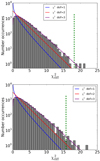 |
Fig. 6. Distributions of |


Results from the Monte Carlo tests used to quantify the chance probability (and related significance) of observing a spectral feature (parameterized with an LP+EP function) on top of the measured VHE gamma-ray spectrum described by an LP.
Additionally, we also performed a Monte Carlo test similar to the one reported in Tombesi et al. (2010), which had been used to quantify the significance of line features obtained from a dedicated search over a large number of measured X-ray spectra. The context of this test is different from the one described above, which relates to the investigation of a feature observed in a single spectrum, but provides an alternative perspective to the evaluation of the random chance probability for the occurrence of narrow features in continuum spectra. The details of this test and the results obtained are given in Appendix D. In addition to the EP function of arbitrary curvature used in the Monte Carlo test described above, we also used an EP function with fixed shape (as in Tombesi et al. 2010) and a Gaussian function of arbitrary width. The results obtained for the three hypotheses are similar, and comparable within 0.5σ, to the results reported in Table 5.
The above-mentioned tests aim to quantify the statistical significance of the deviation of this narrow feature at ∼3 TeV with respect to (smooth) functions typically used to fit the spectra from gamma-ray sources, but they do not account for potential instrumental or analysis problems in the dataset. We performed several tests to search for these instrumental or analysis artifacts that may mimic similar spectral features to the one reported here. Specifically, (a) we performed three different analyses, all them yielding the same results; (b) we inspected the effective area after gamma–hadron separation cuts (see Sect. 3.4 and 4.2 in Aleksić et al. 2016b), which did not show any discontinuity or feature; (c) we varied the gamma–hadron separation cuts (through the random forest hadronness parameter), and several VHE spectra (with different gamma efficiencies) were produced for 2014 July 19, all them showing the feature at ∼3 TeV; (d) we produced spectra with and without the LIDAR atmospheric corrections (Fruck et al. 2015; Furniss et al. 2015), both yielding spectra with the same spectral feature; and (e) we applied the exact same data analysis procedures to data from the Crab nebula taken under similar conditions, yielding a spectrum without features. Therefore, the Mrk 501 VHE spectrum from 2014 July 19, derived in different ways, always showed the narrow TeV feature (at somewhat different magnitudes), deviating from an LP function at a significance varying from ∼2σ to ∼5σ. Therefore, while the narrow spectral feature is statistically only marginally significant (∼3−4σ), we are confident that it is not produced by any instrumental or analysis artifact.
The shape of the VHE spectra from 2014 July 18 and 2014 July 20, above an energy of 1.5 TeV, appears to be compatible with the VHE spectrum from 2014 July 19, as is shown in the bottom panel of Fig. 4. While there is clear variability at energies below 1.5 TeV during these three consecutive nights, the spectral points appear to be similar at energies above 1.5 TeV. Nevertheless, as shown in Table A.3, the spectra obtained from the nights before and after that of July 19 are nicely described with PL functions, and hence the deviations from the PL functions above 1.5 TeV are not significant. Therefore, the sensitivity of these observations with MAGIC is insufficient to constrain the duration of the ∼3 TeV feature to only one day: it may have lasted for three nights, which would correspond to the first of the two bumps in the VHE emission reported in the LC from Fig. 1. We did not find any evidence of narrow spectral features in the VHE spectra during the second bump of the flare (MJD 56865−56867) when a similar X-ray and VHE flux is reached, as shown in Fig. 1.
This is the first time that a narrow VHE spectral feature, inconsistent with a smooth function (PL, LP, and ELP) at more than 3σ, is found in the spectrum of Mrk 501 or any other blazar (see Table 3). With the caveat of doing the test a posteriori, the addition of a narrow component (EP, see Eq. (6)) to the VHE spectral fit is preferred at more than ∼3−4σ, depending on the method used for the test. This additional spectral component peaks at ∼3 TeV with a FWHM of ∼1.4 TeV, and, as we discuss in Sect. 5, it may be interpreted as an indication of additional physics in the theoretical framework aiming to explain the broadband emission of Mrk 501.
4. Characterization of the temporal evolution of the broadband spectral energy distribution
Broadband SEDs were built with MWL simultaneous observations performed within hour timescales: out of the 15 SEDs considered here, the temporal difference between the X-ray and VHE measurements is less than 1 h for six of them, between 1 and 2 h for five of them, and 3 h for two of them. The remaining two SEDs do not have X-ray data taken simultaneously with the VHE data observations, and we used the spectra from the night before and after as a guide. Given that we did not detect significant intra-night variability, we can assume that the variability timescales are longer than the time difference between observations. Therefore, all the observations used here can be considered simultaneous. Each individual MWL SED is modeled using a one-zone SSC model from Tavecchio et al. (1998). The emitting region is assumed to be a sphere filled with relativistic electrons whose radius is compatible with the section of the jet. The electron energy distribution (EED) is described by a smoothed broken power law function as
where K represents the normalization factor, and the spectral indices before and after the break are given by n1 and n2, respectively. The energy (Lorentz factor) break is denoted by γb, and the function is defined between a minimum and maximum Lorentz factor γmin and γmax. The synchrotron emission is produced by the interaction of this relativistic electron distribution with the tangled magnetic field (B). The synchrotron photons can interact with the same population of relativistic electrons via inverse Compton (IC) scattering, being responsible for the high-energy emission within the SSC scenario. In addition, the model also takes into account the bulk Lorentz factor and the viewing angle of the jet, included within a single parameter as the Doppler factor (δ). The emitting region size is constrained by the causality relation: R < (c ⋅ t ⋅ δ)/(1 + z). Assuming a δ = 20, which is often used to model the broadband SED of Mrk 501 within SSC scenarios (e.g., Abdo et al. 2011; Aleksić et al. 2015a), and given that the shortest variability found within the MWL data sample is on the order of one day, the emitting region size can be constrained to R < 5 × 1016 cm.
During the two-week time interval considered in this work, the X-ray emission observed by XRT display very hard spectra, compatible with the historical Mrk 501 flare from 1997 (see, e.g., Tavecchio et al. 2001). Such hard X-ray spectra cannot be properly described together with the optical-UV emission with a single component. A similar situation occurred with the data collected from the extensive campaigns in 2009 and 2012 (Ahnen et al. 2017, 2018). Moreover, as shown in Figs. 1 and 2, the variability observed in the optical-UV band is much lower than in X-rays and VHE gamma rays, which also suggests that the emission at the optical and X-ray frequencies is dominated by different components, possibly located at different parts of the jet.
A study using multi-year radio and optical light curves reported in Lindfors et al. (2016) shows only a marginally significant (2σ confidence level) correlation between these two bands. This suggests that a fraction of the optical emission might be produced co-spatially with the radio emission. Due to self-absorption at radio frequencies, the radio emission is assumed to be produced in the outer regions of the jet. The radio emission is likely produced by a superposition of multiple self-absorbed jet components (Königl 1981). Emitting regions at radio wavelengths are typically larger and more complex. In particular, for Mrk 501 the radio observations reveal a complex jet with multiple components and a jet limb re-brightness (Giroletti et al. 2008). Therefore, the simple one-zone SSC models are not the best approach to model the radio and optical-UV emission. In any case, just as an example, we tried and successfully managed to model the radio to optical–UV emission with an additional SSC component with a larger size. The details are given in Appendix D.
One of the goals of this work is to describe the evolution trend of the MWL SEDs observed during this two-week period of outstanding X-ray activity. Owing to the degeneracy in the parameter values from theoretical models used for blazars, we do not intend to produce model curves that describe perfectly the SEDs, but rather to evaluate how to reproduce the observed broadband behavior with simple variations in the model parameters. For this purpose we attempted to model the data modifying only a few parameters. Given that the overall behavior observed during this period of extreme X-ray activity in 2014 is quite similar to that observed during the outstanding flaring activity in 1997 (Pian et al. 1998; Djannati-Atai et al. 1999; Quinn et al. 1999), we decided to follow Tavecchio et al. (2001), and relate the overall changes in the broadband SED to variations in the parameter γb. In the canonical one-zone SSC scenario, the break in the electron energy distribution is related to the cooling of the electrons and hence inversely related to the size of the emitting region R and the square of the magnetic field B2 (see Appendix F), and hence any modification of γb will come with changes in the parameters R and/or B. For simplicity, we fixed the size of the emitting region, as well as the edges γmin and γmax and the electron number density and Doppler factor δ, and allowed the magnetic field strength B, the indices n1 and n2, and the break γb of the EED to vary. Following the canonical one-zone SSC framework, we also kept the expected difference in the spectral indices n2 − n1 ∼ 1.
The broadband SEDs for 15 consecutive days, together with the one-zone SSC models adjusted to describe the data points, are shown in Fig. 7. The model parameters are reported in Table 6. The agreement between the SED data and the model curves is good, indicating that the adopted strategy to ascribe most of the broadband variations to γb (with adjustments in the parameters B and n1 and n2), as already done in Tavecchio et al. (2001), also works well for the extreme X-ray activity observed in July 2014. Within this framework, the variations in the broadband emission of Mrk 501 may be interpreted as being due to changes in the acceleration and cooling of the electrons in the shock in jet model (see, e.g., Kirk et al. 1998), which would produce substantial variations in the parameter γb, while many of the other model parameters characterizing the emitting region would remain almost stationary. This would naturally explain the existence of large variations close to the peaks of the two SED bumps (X-ray and VHE), while at lower energies (optical and below), where the emission is dominated by a large number of low-energy electrons, the magnitude of the flux variations would be small.
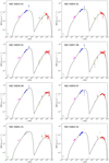 |
Fig. 7. Single-night broadband SEDs described with a one-zone SSC model. The VHE gamma-ray spectra from MAGIC are represented by the red dots, the Fermi-LAT spectra by the black (4 days) and yellow (10 days) triangles, the BAT emission by the blue triangles (using the spectral shape from XRT) and green triangles (using the spectral shape from the stacked BAT analysis over the time interval MJD 56854.5–MJD 56872.5), the binned X-ray spectra from XRT by the blue circles, the optical-UV observations from KVA and UVOT by the pink squares, and the radio observations from Metsähovi by the green squares. Most of the data samples were selected from observations taken within 3 h of each other. For MJD 56861 and MJD 56863 there were no Swift observations taken within the same night of the MAGIC observations, and we depicted the spectra (UVOT, XRT, and BAT) from the night before and the night after with gray symbols. Upper limits are shown as open symbols. See text in Sect. 4 for further details. |
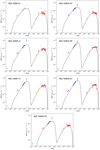 |
Fig. 7. continued. |
One-zone SSC model results.
5. Characterization of the broadband SED with a narrow TeV component
As discussed in Sect. 3.4, an indication of a narrow spectral feature at ∼3 TeV was found in the VHE spectrum of Mrk 501 from 2014 July 19 (observation from MJD 56857.98). This prevents the parameterization of the VHE spectrum with analytic functions typically used to describe the VHE spectra of blazars (e.g., PL, LP). This feature may also be present at some level in the spectra from the day before (MJD 56856.91) and the day after (MJD 56858.98), as shown in Fig. 4, but these two spectra can be fit well with simple power-law functions. It is during these three days when Swift/XRT measured the highest count rates from Mrk 501, which can be seen as the highest fluxes reported in Table A.1 for the energy band 0.3−2 keV8, with the highest X-ray flux observed for the night of July 19−20 (Swift observation from MJD 56858.04), when the VHE spectrum shows the indication for a narrow feature at 3 TeV. However, if we also consider the energy flux emitted in the X-ray band 2−10 keV, the X-ray emission from these three days is comparable to that measured nine days later, during the three consecutive days from July 28 to July 30 (MJD 56866.0, MJD 56867.0, and MJD 56868.0). The VHE gamma-ray activity measured with MAGIC during the three days from July 28 to July 30 is also comparable to that from the three days from July 18 to July 20, with fluxes above 1 C.U. in the energy band 0.15–1 TeV, and fluxes well above 1 C.U. at energies above 1 TeV (see Fig. 1); however, the VHE spectra from July 28−30 do not show any indication of narrow features at TeV energies. Neglecting the potential presence of a feature in the VHE spectra from July 18 and July 20 (which is not significant), out of six VHE spectra with extremely high X-ray emission and (relatively) high VHE gamma-ray emission, the narrow feature is observed in only one VHE spectrum, the one from July 19. If we treat these six observations as similar in terms of X-ray and VHE activity, and assume that the probability of finding a narrow feature in all them is the same, the significance of the narrow feature in the measured VHE spectrum from July 19 should be corrected for six trials. In that case, the ∼3.6σ derived with the Monte Carlo tests reported in Sect. 3.4 (see Table 5) would decrease to ∼3.1σ. We could adopt a more conservative scenario, and treat all 15 observations performed with MAGIC (during this period of enhanced X-ray activity in July 2014) as 15 independent trial factors, which would further decrease the significance to ∼2.8σ. In the most conservative approach, we could consider it equally probable for the many hundreds of Mrk 501 VHE spectra obtained during the last two decades to contain a narrow TeV feature, implying several hundreds of independent trial factors (neglecting any correlation with X-ray and/or VHE activity). The latter approach would naturally make the narrow feature observed on July 19 totally insignificant. Owing to the variable nature of blazars, which show a large diversity of X-ray and VHE spectral behavior over time, often showing outstanding and unexpected behaviors on specific days (i.e., super-large flares, particularly soft or hard spectra), we think it is reasonable to consider the uniqueness of the highest X-ray activity during the July 2014 flare, and hence we think it is reasonable to regard the VHE spectrum from July 19 as special. This would imply that, at most, we should consider only a few trials (instead of tens or hundreds of trials), which would lead to a marginally significant (∼3σ) indication for the presence of a narrow feature at 3 TeV.
There are no reports in the literature about such narrow features in the VHE spectra, but there are broadband SEDs with narrow high-energy bumps, such as the ones measured for Mrk 421 on MJD 55265 and MJD 55266 on March 2010 (see Fig. 8 from Aleksić et al. 2015c) or the one measured for Mrk 501 on MJD 56087 on June 2012 (see Fig. 7 from Ahnen et al. 2018). In those cases the broadband SED was better explained when adding an extra component with a relatively narrow EED. In the literature, we can also find different studies that require extra components to explain broadband SEDs and complex variability patterns. In the case of Mrk 501, with data from 2009, Ahnen et al. (2017) showed, using a grid-scan over the model parameters, that a two-zone scenario was statistically preferred over a one-zone scenario. Multiple zones have also been used in non-HBL blazars. For instance, in the case of the flat-spectrum radio quasar (FSRQ) PKS 1222+21 (also known as 4C +21.35), variability on the order of ∼9 min was found in the VHE band with the MAGIC telescopes (Aleksić et al. 2014c). Such short variability time, together with the absorption of VHE gamma rays within the BLR, suggest that a small emitting region or blob located outside of the BLR is needed to reconcile the findings with the canonical emission models for FSRQs (Tavecchio et al. 2011). Different variability patterns have also been found at different wavelengths, as in the case of the gravitationally lensed blazar QSO B0218+357 (Ahnen et al. 2016), suggesting that more than one emitting region is responsible for the MWL emission.
Under the assumption that the narrow feature in the VHE spectrum of Mrk 501 at ∼3 TeV is real, it is legitimate to investigate theoretical scenarios that could produce it. In this work, we present three different frameworks that would produce broadband SEDs compatible with the observations. One possible explanation for the TeV feature could be the formation of a pileup in the EED due to stochastic acceleration, which would explain the broadband SED using a single region with a multi-component EED. On the other hand, the TeV spectral feature could be produced by the VHE gamma-ray emission from a completely different region. Two scenarios are considered for the latter: SSC emission from a narrow EED in an additional (small) region within the Mrk 501 jet, and emission from electrons accelerated in a magnetospheric vacuum gap close to the supermassive black hole. In the following paragraphs we describe each of the three theoretical approaches.
5.1. Pileup in the electron energy distribution due to stochastic acceleration
Stochastic acceleration has been invoked to explain curved spectra, described by a log-parabolic law, observed in blazar SED (e.g., Massaro et al. 2006, 2008), and the trends between the corresponding peak energy and the trends between the corresponding peak energy and the spectral curvature (Tramacere et al. 2009, 2011). Moreover, stochastic acceleration can also lead to the formation of a pileup in the high-energy range of the relativistic EED (Virtanen & Vainio 2005; Stawarz & Petrosian 2008; Tramacere et al. 2011). Based on this scenario we interpret the sharp and narrow spectral feature observed in the VHE band, together with the high flux level observed by BAT above 10 keV, as the result of a piled-up EED.
As a first approach, we investigate the case of pileup obtained from a continuous mono-energetic injection, escape, and acceleration, under the condition that the particle escape time (tesc) is greater than the dominant acceleration timescale (tacc). Under these circumstances, a pileup will emerge around the equilibrium energy (γeq), i.e., the Lorentz factor that satisfies the condition tcool(γ) = tacc(γ), where tcool is the dominant cooling time. The spectral feature shape is described by a relativistic Maxwellian distribution (Stawarz & Petrosian 2008; Schlickeiser 1985)
![$$ \begin{aligned} n(\gamma )\propto \gamma ^2 \exp {\left[\frac{-1}{f(q,\dot{\gamma })} \left(\frac{\gamma }{\gamma _{\rm eq}}\right)^{f(q,\dot{\gamma })}\right]}, \end{aligned} $$](/articles/aa/full_html/2020/05/aa34603-18/aa34603-18-eq23.gif)
where  is a function depending on the index of the turbulent magnetic field spectrum and on the cooling process. In particular, when the cooling is quadratic in γ,
  . Theoretical scenarios based on multiple blobs with relativistic Maxwellian-type EEDs have been used to explain the very hard gamma-ray spectrum of Mrk 501, as measured with Fermi-LAT (Lefa et al. 2011; Shukla et al. 2016). In this paper we use a single relativistic Maxwellian EED to explain the narrow feature at 3 TeV in the VHE spectrum measured with MAGIC.
In the case of “hard-sphere” turbulence (q = 2.0) the analytical solution for the steady state solution reads (Stawarz & Petrosian 2008)
where γinj is the injection energy, and σ determines the spectral slopes above and below γinj as a function on the ratio ϵ = tacc/tesc and according to  .
.
In order to understand whether this scenario can reproduce the observed SED, it is useful to evaluate the relative normalization of the pileup branch in Eq. (8) (defined for γ ≳ γeq) to the power-law branch (defined for γinj < γ ≪ γeq), at γ = γeq, given by
where Γ is the gamma function. According to Eq. (9), the pileup shape will be significantly dominant over the high-energy power-law branch, only for σ ≲ 1.3, a value that is too hard to reproduce the IC spectrum below the TeV bump, and the X-ray spectrum observed in the XRT window. Hence, we conclude that this scenario is not easily adaptable to our observed data.
A second possible scenario is given by two injection episodes of mono-energetic particles with γinj ≪ γeq, occurring within the same acceleration region, with a duration of  and
and  , respectively, and delayed by a time interval ΔTinj. As long as ΔTinj is larger than a few tacc, the first population of particles will “thermalize” toward a relativistic Maxwellian around γeq (Katarzyński et al. 2006; Tramacere et al. 2011), and these particles will be mostly responsible for the emission in the TeV bump, and in the X-rays above 10 keV.
If the second injection of particles occurs with a delay ΔTinj of a few tesc, then a lower energy branch will develop cospatially with the initial relativistic Maxwellian population. The distribution resulting from the second injection, before and close to the equilibrium, can be described by a power law turning into a log-parabola (LPPL), above a critical energy γ0 (Tramacere et al. 2009, 2011). The phenomenological representation for this scenario can be provided by the following EED:
The first two terms represent the LPPL branch corresponding to the evolution of the second population, and the last term corresponds to the thermalized Maxwellian obtained from the first injection. The parameter s correspond to the σ parameter in Eq. (9), and the parameter r describes the curvature of the LPPL distribution that evolves under the effect of the diffusive component of the acceleration, and the parameter K takes into account the ration between the two injections of particles.
We note that we are ignoring the region of the EED below γinj because, given the parameter space adopted for the modeling, this part of the EED does not impact significantly on the model above the UV frequencies, except that for a normalization factor.
We build two models, a slower cooling model with a value of the magnetic field B = 0.1 G, and a faster cooling model with a higher value of B = 0.3 G, and we refer to them as “slow” and “fast” cooling respectively. We assume a beaming factor of 10, and according to the timescale variability of tvar ≲ one day, we set the constraint on the source size to be R ≤ ctvarδ/(1 + z)≈9 × 1015 cm.
If we take into account the synchrotron cooling alone, the condition for the formation of the Maxwellian bump in the first injection, tcool = tacc, and the value of the best fit γeq ≃ 4 × 10⁵, require values of tacc of ≃2.21 days and ≃0.25 days, for the slow and fast cooling model, respectively. These timescales refer to the rest frame of the emitting-acceleration region, hence in the observer frame will be shortened by a factor of (1 + z)/δ ≃ 0.1. If we combine these requirements on tacc with the constraint that ΔTinj is larger than a few tacc (necessary for the thermalization of the first injection), we conclude that the derived observed timescales are compatible with the temporal behavior observed in the MAGIC and Swift energy range.
The result of our best fit models are shown in Fig. 8 and the corresponding parameter values are reported in Table 7. For the numerical modelling we used the JetSeT9,10 code. The values of the curvature r, for both models, is compatible with a distribution that is approaching the equilibrium (Tramacere et al. 2011), hence we might argue that during the second injection episode the acceleration time has decreased compared to the first injection. For both scenarios investigated in this section we used a value of  , which is compatible with a turbulence index of q = 2. We note that smaller values of q could provide a better description of the narrow bump observed in the TeV spectrum. A more detailed description of this scenario requires a deeper investigation of the temporal evolution of the emitting plasma under the effect of both acceleration and cooling processes through a numerical solution of the corresponding Fokker-Planck equation, and will be presented in a future publication.
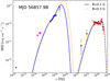 |
Fig. 8. Broadband SED from 2014 July 19 (MJD 56857.98) modeled assuming a pileup in the electron distribution due to stochastic acceleration, and using two different values of the magnetic field: slow cooling with B = 0.1 G and fast cooling with B = 0.3 G. The color-coding for the data points is the same as in Fig. 7. See text in Sect. 5.1 for further details. |
5.2. Additional SSC model component with a narrow electron energy distribution
In this theoretical framework, we used a two-zone SSC model to explain the narrow spectral feature at VHE energies. The second (small) emitting region is added to the first (large) one-zone emitting region. Such a scenario can be envisioned as a jet-in-jet model (see, e.g., Giannios et al. 2009), where a small emitting region or blob is embedded within the jet. Two situations are considered: the two emitting regions are co-spatial (i.e., the second blob is embedded within the standard one-zone region) or the two regions are not co-spatially located. In the case of the co-spatial blob, to avoid a strong interplay between the two regions, the photon density within the small blob needs to be sufficiently high such that the external photon field from the large region is negligible for inverse-Compton scattering and for e+e− pair creation, otherwise the interaction of the relativistic electrons and the emitted gamma rays from the small blob with the synchrotron emission from the large region would broaden and absorb the spectral TeV feature. For the second scenario, with non co-spatial emitting regions, the conditions can be somewhat relaxed, apart from a very low magnetic field required within the small blob. In the non co-spatial scenario the small emitting region should be located farther away from the central engine (closer to the observer) than the larger emitting region to prevent the gamma-ray absorption in the low-energy photon field. The parameters used to describe the large one-zone emitting region (within the two-zone scenario) were slightly modified to prevent the model from overestimating the measured broadband spectra. The parameters are reported in Table 8 and the models can be found in Fig. 9. As shown in Table 8, a large Doppler factor is used, as typically done for jet-in-jet models. Despite the absence of fast (sub-hour) variability, a large Doppler factor is required due to the extremely narrow EED of the small blob. A low (or typical) Doppler factor would require a large (typical) emitting region size, which would imply diffusion, thus making the assumption of a narrow EED unlikely. We note that, due to the large difference in the Doppler factor from the two regions, the co-spatial case would only be possible during a time period on the order of days.
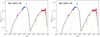 |
Fig. 9. Broadband SED from 2014 July 19 (MJD 56857.98) described with a two-zone SSC model that assumes co-spatial (left panel) and non co-spatial (right panel) locations of the emitting regions within the jet. For both panels, the emission from the small region (with narrow EED) is denoted by the red dot-dashed line, while the sum of the emission from the two regions is depicted by the black solid line. The color-coding for the data points is the same as in Fig. 7. See text in Sect. 5.2 for further details. |
5.3. IC pair cascade induced by electrons accelerated in a magnetospheric vacuum gap
An alternative way to explain the narrow spectral feature at VHE is through the emission resulting from an electromagnetic cascade initiated by electrons accelerated to energies of about 3 TeV in a magnetospheric vacuum gap. In this scenario the electromagnetic cascade, which develops via the interaction of the high-energy electrons with emission line photons from photo-ionized gas clouds, is responsible for the creation of a narrow component of high-energy photons which, after escaping from the interaction region, get superimposed on the SSC emission from a distinct (large) region. Below we show that such a cascade can develop in the central region of Mrk 501, and embody the observed broadband SED from 2014 July 19.
Inverse-Compton (IC) pair cascades were first discussed by Zdziarski (1988) and were recently treated numerically by Wendel et al. (2017). We adopt a refinement of the scenario in the later work for modeling the emission of an electromagnetic cascade (Wendel et al., in prep.). There, the interaction of electrons and positrons (hereafter called electrons) and high-energy photons (HEPs) with a background field of low-energy photons (LEPs) is considered. The LEPs assumed for this scenario are those from the emission of recombination lines from photo-ionized clouds in the inner portion of the host galaxy. We consider only two interaction processes: Breit-Wheeler pair production (PP) and IC-scattering. PP happens solely via collisions of the HEPs with the LEPs, creating electrons that are again available for IC-scattering, and removing the HEPs from their distribution. IC-scattering happens via collisions of relativistic electrons with the LEPs, creating new HEPs that are available for PP, and reducing the energy of the electrons. The interplay of PP and IC-scattering initiates a cascade that evolves the HEP and the electron distributions.
Zdziarski (1988) and Wendel et al. (2017) neglected both electron escape and HEP escape from the interaction region (which would imply an infinitely large interaction volume); in contrast we follow Wendel et al. (in prep.) and include these two additional processes into the scenario. Effectively, this means that the IC pair cascade develops only inside a spherical region of radial size R. The observer detects the HEPs that escape from this interaction region and arrive to Earth. For the mean escape time, we use tesc = R/c with c being the speed of light.
It has been proposed (Levinson & Rieger 2011; Neronov et al. 2012; Ptitsyna & Neronov 2016) that there are charge-depleted regions near the poles of the magnetospheres of spinning black holes. These so-called vacuum gaps exhibit a strong electric field component, which is directed along the magnetic field. Thus, if charged particles enter the gap from the accretion disk, or are created there via PP by photons from an accretion flow, then these charged particles can be accelerated to ultra-relativistic energies and can initiate an IC pair cascade. It is thus justified to approximate the injected relativistic electron distribution (Ṅi(γ)) per unit space volume by a Gaussian distribution:
Here the normalization of the Gaussian (KG) describes the total number of electrons per unit space volume and per unit time interval that are accelerated in the vacuum gap, propagate away from the vacuum gap along the Mrk 501 jet axis, and penetrate into the cascade interaction region. The cutoff in Ṅi below γi, 1 and above γi, 0 was introduced to satisfy the condition γ ⋅ x > 1, where x is the LEP energy divided by the electron rest energy (Zdziarski 1988; Wendel et al. 2017). We chose γi, 1 = γmean − 3.0σ and γi, 0 = γmean + 3.0σ.
Even though Mrk 501 is classified as a BL Lac-type object and has no pronounced BLR, it is probable that gas clouds from the inner portion of the host galaxy intrude into the AGN. These gas clouds, which stem from the interstellar medium and thus consist mainly of hydrogen and helium (Wilms et al. 2000), are photo-ionized by the energetic radiation from hot stars and/or the accretion flow. Emission of recombination lines by the photo-ionized gas clouds is thus inevitable. This leads to abundant emission line photon fields in the AGN. Hence, the spectral number density of the LEPs (n0(x)) can be described by a sum of Delta functions
The Delta functions are situated at the energy x0, i = h/(λ0, i me c), where h, λ0, i, and me are the Planck constant, the wavelength of line i, and the electron rest mass, respectively. The parameter Kline, i describes the relative flux of the ith emission line. Dividing Kline, i by the energy x0, i of the respective line, gives the relative contribution to the number density. The parameter Klines determines the total number density of LEPs. We include these four lines here, which are generally the most prominent ones in broad-line region spectra (Pian et al. 2005) and synthetic photo-ionization spectra (Abolmasov & Poutanen 2017), and list them in Table 9. In the following model we do not pay attention to photons from the accretion flow because the demand to synthesize a sharp feature can be met best by usage of a sharp distribution of LEPs. If electrons from the vacuum gap penetrate into the field of emission line photons, they interact with the LEPs and initiate an IC pair cascade, which will create HEPs and secondary electrons.
The kinetic equation that describes this type of cascade, and the numerical scheme to solve it iteratively to obtain electron and HEP spectral number densities N(γ) and nγ(xγ), with xγ being the HEP energy divided by the electron rest energy, is described in Wendel et al. (in prep.). The HEP spectral number density is determined as the ratio of the IC production rate of HEPs to the loss rate of HEPs, which is the sum of the escape rate and the attenuation rate due to pair absorption. Because of the scattering kinematics, the HEPs leave the volume within a beam of opening angle ϕ in the direction the electrons entered the interaction region. The spectral number of photons that stream through a unit area per unit time interval and can be detected at Earth is
where nγ is measured in units of mec2. The luminosity distance D = 149.4 Mpc, and Ω(ϕ) is the solid angle of the HEP beam with conical shape and opening angle ϕ.
The resulting spectrum is, after adding the one-zone SSC model shown in Fig. 7, adjusted to the narrow SED peak from 2014 July 19. With the parameters listed in Table 10, the narrow feature can be theoretically explained, as is shown in Fig. 10, by emission line photons that have been IC upscattered by the electrons from the gap.
 |
Fig. 10. Broadband SED from 2014 July 19 (MJD 56857.98) modeled with one-zone SSC emission (gray dashed and gray dot-dashed lines) and the emission from an IC pair cascade (red dot-dashed line). The sum of the two components is depicted by the black solid line. The color-coding for the data points is the same as in Fig. 7. See text in Sect. 5.3 for further details. |
The large dip in the cascaded spectrum above 1025 Hz, and the small dip above 1024 Hz, are due to the absorption of HEPs due to PP with LEPs from the hydrogen Lyman α line and helium II Lyman α line, respectively11. Consequently, the bump at 1024 Hz is due to cascaded emission that is just below the PP threshold, and thus not pair absorbed. The cascaded HE radiation stems from a region that is located within the typical extent of a BLR. Mrk 501 has no detectable BLR, and hence the density of LEPs must be low, and probably dominated by emission lines from photo-ionized hydrogen and helium gas clouds that stem from the interstellar medium. The density of LEPs is such that the cascade is well sustained, but the HE photons are not entirely pair absorbed, and can escape and be detected by the MAGIC telescopes. This is in contrast to the case of LBLs and FSRQs, where it is usually considered that the density of LEPs is large, and the HE radiation originating from inside the BLR is completely pair absorbed, implying that the HE radiation sometimes (e.g., during large flares) detected for some of these objects has to originate from outside the BLR (see, e.g., Aleksić et al. 2014c; Ahnen et al. 2016). A discussion on the implications of the used parameters on the physical state of Mrk 501 can be found in Wendel et al. (in prep.).
Within the theoretical framework presented here, the narrow feature detected with MAGIC in the VHE spectrum of Mrk 501 is interpreted as a signature of electron acceleration in a magnetospheric vacuum gap, close to the supermassive black hole. Similar theoretical scenarios were also used to explain the fast variability in radio galaxies (e.g., Aleksić et al. 2014b; MAGIC collaboration 2018), and to test the stability of a gap and the resulting radiation on a theoretical basis (Ptitsyna & Neronov 2016; Hirotani & Pu 2016). The main difference with respect to those scenarios is that, in the study presented here, the inverse-Compton scattering occurs on emission line photons from BLR-like clouds, and dominate the broadband gamma-ray emission only in a narrow range of energies. In other published works, the inverse-Compton scattering occurs on seed photons emitted by the accretion disk, and describes a large fraction of the entire gamma-ray emission. From the technical perspective, another difference is that in this work we neglect curvature radiation due to its minor importance for the electron energy loss rate (Levinson & Rieger 2011), and that we use the electron energy distribution N(γ) as a fitting function, whereas in the model by Hirotani & Pu (2016) the electron energy distribution is an inherent feature of the existence and stability of the gap.
6. Summary and concluding remarks
We presented observational and theoretical results derived with multi-instrument data from Mrk 501 collected during a ∼two-week period in July 2014, when the X-ray activity was at its highest among the ∼14 years of operation of the Neil Gehrels Swift Gamma-ray Burst Observatory. During this outburst, the X-ray spectra measured with XRT (and with BAT) were very hard, and somewhat similar to the large historical flare from 1997 that was measured with BeppoSAX beyond 100 keV (Pian et al. 1998).
During this short time interval, the flux variations in the radio, optical, and GeV bands were rather mild (Fvar ∼ 0.05), but quite substantial in the X-ray bands (Fvar > 0.15) and especially substantial in the VHE bands (Fvar > 0.3). No intra-night variability was observed on any of the nights. There is a general increase in the fractional variability with energy, with the highest variability occurring at VHE. This variability pattern is similar to that from other multi-wavelength campaigns targeting Mrk 501 (Aleksić et al. 2015a; Aliu et al. 2016; Ahnen et al. 2017, 2018), but very different from the behavior observed in Mrk 421, which shows a clear double-bump structure with the highest variability often observed at X-ray energies (Aleksić et al. 2015b,c; Baloković et al. 2016). The correlation between the X-ray and VHE bands (the most variable segments of the electromagnetic spectrum), was investigated using two energy ranges for each, namely 0.3–2 keV and 2–10 keV for X-rays, and 0.15–1 TeV and > 1 TeV for VHE. This study shows, for the first time for Mrk 501, a significant correlation (>3σ) between these two bands during a relatively short time interval (∼2 weeks) with a persistent elevated activity. Moreover, we observed that the strength and the significance of this correlation increases with increasing energy in X-rays, similarly to what was reported by Ahnen et al. (2018) using the dataset of a few months in length from 2012.
During the X-ray flux peak, we observed a narrow feature at about 3 TeV in the VHE gamma-ray spectrum measured with the MAGIC telescopes on 2014 July 19 (observation performed at MJD 56857.98). This TeV feature cannot be described with the analytic functions typically used for the VHE spectra of blazars, such as power laws, log-parabolas, and log-parabolas with exponential cutoffs: the inconsistencies are larger than ∼3σ. A fit with a log-parabola below 1.5 TeV and extrapolated to higher energies shows deviations with the data of 4–5σ. A likelihood ratio test shows that a log-parabola with an additional narrow component (modeled with another log-parabola with a strong curvature) is preferred with respect to the single log-parabola at more than 4σ. In addition, a dedicated Monte Carlo simulation indicates the presence of the narrow component at a significance larger than 3σ. This narrow TeV feature may also be present at some level in the spectra from the earlier (July 18) and later (July 20) nights, but at much lower significance. While the VHE spectra of Mrk 501 have previously shown a prominent peaky structure (see, e.g., Fig. 7 in Ahnen et al. 2018), this is the first time that such a narrow feature has been observed, even if only at a marginally significant level of ∼3–4σ.
A detailed study on the temporal evolution of the broadband SEDs from 2014 July 16 (MJD 56854.9) to 2014 July 31 (MJD 56869.9), resolved on a day-by-day basis, was performed. The time difference between the X-ray and VHE data is mostly below 3 h which, given the lack of variability on hour timescales, can be considered as simultaneous observations. The daily evolution of the most variable segments of the SED, namely the X-ray and the gamma-ray bands, which is where the most energy is emitted, could be successfully parameterized with a one-zone SSC model, where the main variations are produced by changes in the break energy γb, with some adjustments in the parameters B, n1, and n2. Within this theoretical framework, these results suggest that the flux variations on timescales of days are produced by the acceleration and the cooling of the high-energy electrons.
The SED from 2014 July 19 shows the largest disagreement with the one-zone SSC, which is due to the narrow feature at ∼3 TeV observed in the MAGIC spectrum. Under the assumption that this spectral feature is real, we investigated three theoretical scenarios that could reproduce it: (a) pileup in the electron energy distribution due to stochastic acceleration; (b) a structured jet with two-SSC emitting regions (related or not related), with one region dominated by an extremely narrow electron energy distribution; and (c) an emission produced via an IC pair cascade induced by electrons accelerated in a magnetospheric vacuum gap, in addition to the SSC emission from a more conventional region along the jet of Mrk 501. The three frameworks could reproduce the narrow spectral component reasonably well, given its relatively large uncertainties. Future observations of the gamma-ray emission of Mrk 501 and other bright VHE blazars will help investigate the reliability and potential recurrence of narrow spectral components.
Moreover, these spectral features may also occur at hard X-rays, as predicted by the theoretical scenario from Sect. 5.1. Therefore, observations with high-resolution hard X-ray instruments like NuSTAR, together with current and future Cherenkov telescopes such as CTA, would allow for a better characterization of narrow spectral features in both the low- and high-energy bumps, which could have important implications for the understanding of particle acceleration and radiation in Mrk 501, and in blazars in general.
Acknowledgments
The authors thank the anonymous referee for providing a constructive list of remarks that allowed us to clarify and improve some of the results reported in the manuscript. We would like to thank the Instituto de Astrofísica de Canarias for the excellent working conditions at the Observatorio del Roque de los Muchachos in La Palma. The financial support of the German BMBF and MPG, the Italian INFN and INAF, the Swiss National Fund SNF, the ERDF under the Spanish MINECO (FPA2015-69818-P, FPA2012-36668, FPA2015-68378-P, FPA2015-69210-C6-2-R, FPA2015-69210-C6-4-R, FPA2015-69210-C6-6-R, AYA2015-71042-P, AYA2016-76012-C3-1-P, ESP2015-71662-C2-2-P, FPA2017-90566-REDC), and the Japanese JSPS and MEXT is gratefully acknowledged. This work was also supported by the Spanish Centro de Excelencia “Severo Ochoa” SEV-2016-0588 and SEV-2015-0548, and Unidad de Excelencia “María de Maeztu” MDM-2014-0369, by the Croatian Science Foundation (HrZZ) Project IP-2016-06-9782 and the University of Rijeka Project 13.12.1.3.02, by the DFG Collaborative Research Centers SFB823/C4 and SFB876/C3, the Polish National Research Centre grant UMO-2016/22/M/ST9/00382 and by the Brazilian MCTIC, CNPq and FAPERJ. The Fermi-LAT Collaboration acknowledges generous ongoing support from a number of agencies and institutes that have supported both the development and the operation of the LAT as well as scientific data analysis. These include the National Aeronautics and Space Administration and the Department of Energy in the United States, the Commissariat à l’Energie Atomique and the Centre National de la Recherche Scientifique/Institut National de Physique Nucléaire et de Physique des Particules in France, the Agenzia Spaziale Italiana and the Istituto Nazionale di Fisica Nucleare in Italy, the Ministry of Education, Culture, Sports, Science and Technology (MEXT), High Energy Accelerator Research Organization (KEK) and Japan Aerospace Exploration Agency (JAXA) in Japan, and the K. A. Wallenberg Foundation, the Swedish Research Council and the Swedish National Space Board in Sweden. Additional support for science analysis during the operations phase is gratefully acknowledged from the Instituto Nazionale di Astrofisica in Italy and the Centre National d’Études Spatiales in France. The important contributions from ETH Zurich grants ETH-10.08-2 and ETH-27.12-1 as well as the funding by the Swiss SNF and the German BMBF (Verbundforschung Astro- und Astroteilchenphysik) and HAP (Helmoltz Alliance for Astroparticle Physics) are gratefully acknowledged. Part of this work is supported by Deutsche Forschungsgemeinschaft (DFG) within the Collaborative Research Center SFB 876, project C3. We thank the Instituto de Astrofisica de Canarias for allowing us to operate the telescope at the Observatorio del Roque de los Muchachos in La Palma, the Max-Planck-Institut fur Physik for providing us with the mount of the former HEGRA CT3 telescope, and the MAGIC Collaboration for their support. JBG acknowledges the support of the Viera y Clavijo program funded by ACIISI and ULL. C. W. is grateful for the support by the project “Promotion inklusive” of the Universität zu Köln and the German Bundesministerium für Arbeit und Soziales. This publication makes use of data obtained at Metsähovi Radio Observatory, operated by Aalto University, Finland.
References
- Abdo, A. A., Ackermann, M., Ajello, M., et al. 2011, ApJ, 727, 129 [NASA ADS] [CrossRef] [Google Scholar]
- Abolmasov, P., & Poutanen, J. 2017, MNRAS, 464, 152 [NASA ADS] [CrossRef] [Google Scholar]
- Acciari, V., Ansoldi, S., Antonelli, L. A., et al. 2019, MNRAS, 486, 4233 [NASA ADS] [CrossRef] [Google Scholar]
- Acero, F., Ackermann, M., Ajello, M., et al. 2015, ApJS, 218, 23A [NASA ADS] [CrossRef] [Google Scholar]
- Ahnen, M. L., Ansoldi, S., Antonelli, L. A., et al. 2016, A&A, 595, A98 [NASA ADS] [CrossRef] [EDP Sciences] [Google Scholar]
- Ahnen, M. L., Ansoldi, S., Antonelli, L. A., et al. 2017, A&A, 603, A31 [NASA ADS] [CrossRef] [EDP Sciences] [Google Scholar]
- Ahnen, M. L., Ansoldi, S., Antonelli, L. A., et al. 2018, A&A, 620, A181 [NASA ADS] [CrossRef] [EDP Sciences] [Google Scholar]
- Anderhub, H., Backes, M., Biland, A., et al. 2013, J. Instrum., 8, P06008 [CrossRef] [Google Scholar]
- Albert, J., Aliu, E., Anderhub, H., et al. 2007, ApJ, 669, 862 [NASA ADS] [CrossRef] [Google Scholar]
- Aleksić, J., Ansoldi, S., Antonelli, L. A., et al. 2014a, A&A, 572, A121 [NASA ADS] [CrossRef] [EDP Sciences] [Google Scholar]
- Aleksić, J., Ansoldi, S., Antonelli, L. A., et al. 2014b, Science, 346, 1080 [NASA ADS] [CrossRef] [Google Scholar]
- Aleksić, J., Antonelli, L. A., Antoranz, P., et al. 2014c, ApJ, 730, L8 [Google Scholar]
- Aleksić, J., Ansoldi, S., Antonelli, L. A., et al. 2015a, A&A, 573, A50 [NASA ADS] [CrossRef] [EDP Sciences] [Google Scholar]
- Aleksić, J., Ansoldi, S., Antonelli, L. A., et al. 2015b, A&A, 576, A126 [NASA ADS] [CrossRef] [EDP Sciences] [Google Scholar]
- Aleksić, J., Ansoldi, S., Antonelli, L. A., et al. 2015c, A&A, 578, A22 [NASA ADS] [CrossRef] [EDP Sciences] [Google Scholar]
- Aleksić, J., Ansoldi, S., Antonelli, L. A., et al. 2016a, Astropart. Phys., 72, 61 [NASA ADS] [CrossRef] [Google Scholar]
- Aleksić, J., Ansoldi, S., Antonelli, L. A., et al. 2016b, Astropart. Phys., 72, 76 [NASA ADS] [CrossRef] [Google Scholar]
- Aliu, E., Archambault, S., Archer, A., et al. 2016, A&A, 594, A76 [NASA ADS] [CrossRef] [EDP Sciences] [Google Scholar]
- Baloković, M., Paneque, D., Madejski, G., et al. 2016, ApJ, 819, 156 [NASA ADS] [CrossRef] [Google Scholar]
- Biland, A., Bretz, T., Buß, J., et al. 2014, J. Instrum., 9, P10012 [CrossRef] [Google Scholar]
- Baumgartner, W. H., Tueller, J., Markwardt, C. B., et al. 2013, ApJS, 207, 19 [NASA ADS] [CrossRef] [EDP Sciences] [Google Scholar]
- Breeveld, A. A., Landsman, W., Holland, S. T., et al. 2011, Am. Inst. Phys. Conf. Ser., 1358, 373 [NASA ADS] [CrossRef] [Google Scholar]
- Burrows, D. N., Hill, J. E., Nousek, J. A., et al. 2005, Space Sci. Rev., 120, 165 [NASA ADS] [CrossRef] [Google Scholar]
- Catanese, M., Bradbury, S. M., Breslin, A. C., et al. 1997, ApJ, 487, L143 [NASA ADS] [CrossRef] [Google Scholar]
- Djannati-Atai, A., Piron, F., Barrau, A., et al. 1999, A&A, 350, 17 [NASA ADS] [Google Scholar]
- Domínguez, A., Primack, J. R., Rosario, D. J., et al. 2011, MNRAS, 410, 2556 [NASA ADS] [CrossRef] [Google Scholar]
- Dorner, D., Biland, A., Bretz, T., et al. 2013, in 33rd International Cosmic Ray Conference, held 2–9 July 2013 in Rio de Janeiro, Brazil, ed. A. Saa, 1093 [Google Scholar]
- Dorner, D., Ahnen, M. L., Bergmann, M., et al. 2015, 2014 Fermi Symposium proceedings – eConf C14102.1 [arXiv:1502.02582] [Google Scholar]
- Edelson, R. A., & Krolik, J. H. 1988, ApJ, 333, 646 [NASA ADS] [CrossRef] [Google Scholar]
- Fitzpatrick, E. L. 1999, PASP, 111, 63 [NASA ADS] [CrossRef] [Google Scholar]
- Furniss, A., Noda, K., Boggs, S., et al. 2015, ApJ, 812, 65 [NASA ADS] [CrossRef] [Google Scholar]
- Fruck, C., Gaug, M., Zanin, Z., et al. 2015, ArXiv e-prints [arXiv:1403.3591] [Google Scholar]
- Gehrels, N., Chincarini, G., Giommi, P., et al. 2004, ApJ, 611, 1005 [NASA ADS] [CrossRef] [Google Scholar]
- Giannios, D., Uzdensky, D. A., & Begelman, M. C. 2009, MNRAS, 395, L29 [NASA ADS] [CrossRef] [Google Scholar]
- Giroletti, M., Giovannini, G., Cotton, W. D., et al. 2008, A&A, 488, 905 [NASA ADS] [CrossRef] [EDP Sciences] [Google Scholar]
- Gliozzi, M., Sambruna, R. M., Jung, I., et al. 2006, ApJ, 646, 61 [NASA ADS] [CrossRef] [Google Scholar]
- Hildebrand, D., Ahnen, M. L., Balbo, M., et al. 2017, Proceedings of ICRC 2017, https://pos.sissa.it/301/779 [Google Scholar]
- Hirotani, K., & Pu, H.-Y. 2016, ApJ, 818, 50 [NASA ADS] [CrossRef] [Google Scholar]
- Kalberla, P. M. W., Burton, W. B., Hartmann, D., et al. 2005, A&A, 440, 775 [NASA ADS] [CrossRef] [EDP Sciences] [Google Scholar]
- Katarzyński, K., Ghisellini, G., Mastichiadis, A., Tavecchio, F., & Maraschi, L. 2006, A&A, 453, 47 [NASA ADS] [CrossRef] [EDP Sciences] [Google Scholar]
- Kirk, J. G., Rieger, F. M., & Mastichiadis, A. 1998, A&A, 333, 452 [NASA ADS] [Google Scholar]
- Königl, A. 1981, ApJ, 243, 700 [NASA ADS] [CrossRef] [Google Scholar]
- Lefa, E., Aharonian, F. A., & Rieger, F. M. 2011, ApJ, 743, L19 [NASA ADS] [CrossRef] [Google Scholar]
- Levinson, A., & Rieger, F. 2011, ApJ, 730, 123 [NASA ADS] [CrossRef] [Google Scholar]
- Li, T.-P., & Ma, Y.-Q. 1983, ApJ, 272, 317 [NASA ADS] [CrossRef] [Google Scholar]
- Lindfors, E. J., Hovatta, T., Nilsson, K., et al. 2016, A&A, 593, A98 [NASA ADS] [CrossRef] [EDP Sciences] [Google Scholar]
- Mahlke, M., Bretz, T., Adam, J., et al. 2017, Proceedings of ICRC 2017, https://pos.sissa.it/301/612 [Google Scholar]
- MAGIC collaboration (Ansoldi, S., et al.) 2018, A&A, 617, A91 [NASA ADS] [CrossRef] [EDP Sciences] [Google Scholar]
- Markwardt, C. B., Tueller, J., Skinner, G. K., et al. 2005, ApJ, 633, L77 [NASA ADS] [CrossRef] [Google Scholar]
- Maraschi, L., & Tavecchio, F. 2003, ApJ, 593, 667 [NASA ADS] [CrossRef] [Google Scholar]
- Maraschi, L., Ghisellini, G., & Celotti, A. 1992, ApJ, 397, L5 [NASA ADS] [CrossRef] [Google Scholar]
- Markwardt, C. B., Barthelmy, S. D., Cummings, J. C., et al. 2007, http://swift.gsfc.nasa.gov/analysis/bat_swguide_v6_3.pdf [Google Scholar]
- Massaro, E., Tramacere, A., Perri, M., Giommi, P., & Tosti, G. 2006, A&A, 448, 861 [NASA ADS] [CrossRef] [EDP Sciences] [Google Scholar]
- Massaro, F., Tramacere, A., Cavaliere, A., Perri, M., & Giommi, P. 2008, A&A, 478, 395 [NASA ADS] [CrossRef] [EDP Sciences] [Google Scholar]
- Mattox, J. R., Bertsch, D. L., Chiang, J., et al. 1996, ApJ, 461, 396 [NASA ADS] [CrossRef] [Google Scholar]
- Markowitz, A., Reeves, J. N., & Braito, V. 2006, ApJ, 646, 783 [NASA ADS] [CrossRef] [Google Scholar]
- Neronov, A., Semikoz, D., & Taylor, A. M. 2012, A&A, 541, A31 [NASA ADS] [CrossRef] [EDP Sciences] [Google Scholar]
- Nilsson, K., Pasanen, M., Takalo, L. O., et al. 2007, A&A, 475, 199 [NASA ADS] [CrossRef] [EDP Sciences] [Google Scholar]
- Nilsson, K., Lindfors, E., Takalo, L. O., et al. 2018, A&A, 620, A185 [NASA ADS] [CrossRef] [EDP Sciences] [Google Scholar]
- Pian, E., Vacanti, G., Tagliaferri, G., et al. 1998, ApJ, 492, L17 [NASA ADS] [CrossRef] [Google Scholar]
- Pian, E., Falomo, R., & Treves, A. 2005, MNRAS, 361, 919 [NASA ADS] [CrossRef] [Google Scholar]
- Poole, T. S., Breeveld, A. A., Page, M. J., et al. 2008, MNRAS, 383, 627 [NASA ADS] [CrossRef] [Google Scholar]
- Poutanen, J., Zdziarski, A. A., & Ibragimov A., 2008, MNRAS, 389, 1427 [NASA ADS] [CrossRef] [Google Scholar]
- Press, W. H., Teukolsky, S. A., Vetterling, W. T., & Flannery, B. P. 2002, Numerical Recipes in C++: The Art of Scientific Computing [Google Scholar]
- Protassov, R., van Dyk, D. A., Connors, A., Kashyap, V. L., & Siemiginowska, A. 2002, ApJ, 571, 545 [NASA ADS] [CrossRef] [Google Scholar]
- Ptitsyna, K., & Neronov, A. 2016, A&A, 593, A8 [NASA ADS] [CrossRef] [EDP Sciences] [Google Scholar]
- Quinn, J., Akerlof, C. W., Biller, S., et al. 1996, ApJ, 456, L83 [NASA ADS] [CrossRef] [MathSciNet] [Google Scholar]
- Quinn, J., Bond, I. H., Boyle, P. J., et al. 1999, ApJ, 518, 693 [NASA ADS] [CrossRef] [Google Scholar]
- Roming, P. W. A., Kennedy, T. E., Mason, K. O., et al. 2005, Space Sci. Rev., 120, 95 [NASA ADS] [CrossRef] [Google Scholar]
- Sambruna, R. M., Aharonian, F. A., Krawczynski, H., et al. 2000, A&A, 538, 127 [Google Scholar]
- Schlafly, E. F., & Finkbeiner, D. P. 2011, ApJ, 737, 103 [NASA ADS] [CrossRef] [Google Scholar]
- Schlickeiser, R. 1985, A&A, 143, 431 [NASA ADS] [Google Scholar]
- Shukla, A., Mannheim, K., Chitnis, V. R., et al. 2016, ApJ, 832, 177 [NASA ADS] [CrossRef] [Google Scholar]
- Stawarz, Ł., & Petrosian, V. 2008, ApJ, 681, 1725 [NASA ADS] [CrossRef] [Google Scholar]
- Tavecchio, F., Maraschi, L., & Ghisellini, G. 1998, ApJ, 509, 608 [NASA ADS] [CrossRef] [Google Scholar]
- Tavecchio, F., Maraschi, L., Pian, E., et al. 2001, ApJ, 554, 725 [NASA ADS] [CrossRef] [Google Scholar]
- Tavecchio, F., Becerra-Gonzalez, J., Ghisellini, G., et al. 2011, A&A, 534, A86 [NASA ADS] [CrossRef] [EDP Sciences] [Google Scholar]
- Teraesranta, H., Tornikoski, M., Mujunen, A., et al. 1998, A&AS, 132, 305 [NASA ADS] [CrossRef] [EDP Sciences] [Google Scholar]
- Tombesi, F., Cappi, M., Reeves, J. N., et al. 2010, A&A, 521, A57 [NASA ADS] [CrossRef] [EDP Sciences] [Google Scholar]
- Tramacere, A., Giommi, P., Perri, M., et al. 2007, A&A, 467, 501 [NASA ADS] [CrossRef] [EDP Sciences] [Google Scholar]
- Tramacere, A., Giommi, P., Perri, M., Verrecchia, F., & Tosti, G. 2009, A&A, 501, 879 [NASA ADS] [CrossRef] [EDP Sciences] [Google Scholar]
- Tramacere, A., Massaro, E., & Taylor, A. M. 2011, ApJ, 739, 66 [NASA ADS] [CrossRef] [Google Scholar]
- Vaughan, S., Edelson, R., Warwick, R. S., & Uttley, P. 2003, MNRAS, 345, 1271 [NASA ADS] [CrossRef] [Google Scholar]
- Villata, M., & Raiteri, C. M. 1999, A&A, 347, 30 [NASA ADS] [Google Scholar]
- Villata, M., Raiteri, C. M., Lanteri, L., et al. 1998, A&AS, 130, 305 [NASA ADS] [CrossRef] [EDP Sciences] [MathSciNet] [PubMed] [Google Scholar]
- Virtanen, J. J. P., & Vainio, R. 2005, ApJ, 621, 313 [NASA ADS] [CrossRef] [Google Scholar]
- Wendel, C., Glawion, D., Shukla, A., & Mannheim, K. 2017, in 6th International Symposium on High Energy Gamma-Ray Astronomy, Am. Inst. Phys. Conf. Ser., 1792 [Google Scholar]
- Wilms, J., Allen, A., & McCray, R. 2000, ApJ, 542, 914 [NASA ADS] [CrossRef] [Google Scholar]
- Zanin, R., Carmona, E., Sitarek, J., et al. 2013, Proceedings of 33rd ICRC, Rio de Janeiro, Brazil, 773 [Google Scholar]
- Zdziarski, A. A. 1988, ApJ, 335, 786 [NASA ADS] [CrossRef] [Google Scholar]
Appendix A: Tables with the X-ray and VHE gamma-ray spectral results
The X-ray spectral fits to the Swift/XRT data from 0.3 keV to 10 keV with a PL and an LP function are reported in Table A.1. The results from Swift/BAT analysis for the one-day time intervals are reported in Table A.2.
The VHE gamma-ray spectral fits to the MAGIC data from 0.1 TeV to 10 TeV (for both observed and EBL-corrected) with a PL and an LP function are reported in Table A.3.
Spectral parameters for the Swift/XRT data from Mrk 501 in the energy range 0.3–10 keV during the high activity in July 2014.
Swit-BAT results from the analysis of Mrk 501 in the energy band 14–195 keV for one-day integration bins.
Spectral parameters for the MAGIC data from Mrk 501 in the energy range 0.1–10 TeV during the high activity in July 2014.
Appendix B: X-ray and VHE gamma-ray spectral index vs. flux
The PL spectral index as a function of the integral fluxes in two energy bands in X-rays and VHE are reported in Figs. B.1 and B.2. The LP function is more suitable than the PL function in a few X-ray spectra and VHE spectra, but the difference is small (see Appendix A). For the sake of simplicity, we decided to use the PL index for the study presented here. The only spectrum that was not considered in this study (for the VHE gamma-ray band) is that from 2014 July 19, which is the one showing a narrow spectral feature at about 3 TeV (see Sect. 3.4).
No correlation is found between the PL spectral index and the VHE fluxes, with Pearson coefficients of 0.30 (1.0σ) and 0.50 (1.7σ) for the energy bands 0.15−1 TeV and > 1 TeV, respectively. On the contrary, the X-ray band shows evidence for the harder-when-brighter behavior, with Pearson coefficients of 0.61 (2.4σ) and 0.86 (4.3σ), and DCF = 0.6 ± 0.3 and DCF = 0.8 ± 0.3, for the soft (0.3–2 keV) and the hard (2–10 keV) X-ray bands, respectively.
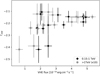 |
Fig. B.1. PL spectral index as a function of the integral flux, as observed by MAGIC in the energy bands 0.15–1 TeV and >1 TeV. |
 |
Fig. B.2. PL spectral index as a function of the integral flux, as observed by XRT in the energy bands from 0.3−2 keV and 2−10 keV. |
Appendix C: Evaluation of extrapolation of LP spectral fit beyond 1.5 TeV
In order to test the behavior of the low- and high-energy part of the VHE spectrum during the two-week period with outstanding X-ray activity, we performed the following test. The spectral data were fit with an LP function up to 1.5 TeV. The value of 1.5 TeV is right below the energy of the narrow spectral feature at ∼3 TeV in the spectrum from 2014 July 19. Afterwards, the data-model agreement was quantified above 1.5 TeV for the extrapolation (to higher energies) of the best-fit function up to 1.5 TeV. The results from these spectral fits, and the quantification of the data-model agreement above 1.5 TeV, are reported in Table C.1.
Results from the forward-folding fits with an LP up to 1.5 TeV to the single-night MAGIC VHE spectra that contains at least three spectral points beyond 1.5 TeV.
As shown in the table, in general, the extrapolation of the fit up to 1.5 TeV provides a good description of the spectral shape at energies above 1.5 TeV. The only notable exception is the spectrum from 2014 July 19 (MJD 56857.98), where there is a significant deviation (from the LP function) at energies above 1.5 TeV. The VHE spectrum from July 20 (MJD 56858.98) also shows a marginally significant deviation at high energies with respect to the fit at low energies.
If we consider the 1σ uncertainty in the best fit up to 1.5 TeV (uncertainty in the spectral parameters reported in Table C.1), the significance of the deviation of the data points with respect to the extrapolation of the spectral fit below 1.5 TeV decreases to a 3σ level for 2014 July 19. For the observed spectrum we find that  /d.o.f. = 24.4/7 (3.3σ), while for the EBL-corrected spectrum the values are
  /d.o.f. = 19.5/7 (2.7σ).
Appendix D: Additional Monte Carlo tests to estimate the chance probability of obtaining a narrow spectral feature on the top of smooth gamma-ray spectra
In this section we describe additional Monte Carlo tests that were performed to assess the random chance probability of obtaining a narrow spectral feature like the one observed in the measured VHE gamma-ray spectrum of Mrk 501 from 2014 July 19 (see Sect. 3.4). In this case, we followed the prescriptions from Tombesi et al. (2010), which had been used to select line-features at pvalue < 0.05 in a systematic search over a large number of measured X-ray spectra. The nature of this test is different from the one described Sect. 3.4, which relates to the investigation of a feature observed in a single spectrum, but provides an alternative perspective to the evaluation of the random chance probability for the occurrence of narrow features in continuum spectra. The tests are performed on the differential flux spectrum (dN/dE) without applying any correction for the EBL. The continuum model (which is taken as the null hypothesis) is described with an LP function, and three distinct functions are used to parameterize the narrow feature: (a) an EP function (see Eq. (6)) with curvature fixed to β = 9.1; (b) a more generic EP function with variable curvature, where β is allowed to change from 1 to 20 in the spectral fits; and (c) a Gaussian function with variable width where sigma is allowed to change from 10% to 40% of the Gaussian mean. The location of the narrow feature (Ep in the EP function, and the mean of the Gaussian function) is determined from a scan over a 40-bin grid extending from the energy 0.08 TeV (first data point in the spectrum) to the energy 6.80 TeV (last data point in the spectrum), in steps of 0.05 in base-10 logarithmic space. Each step corresponds to a relative change in the energy of ∼12%, which is comparable to the energy resolution of MAGIC (15%–20%; see Aleksić et al. 2016b). The narrow feature hypothesis (a) is described with one additional free (and unconstrained) parameter, the normalization K, which can take positive and negative values, and follows the prescriptions from Tombesi et al. (2010). On the other hand, hypotheses (b) and (c) relate to a more generic search where the spectral feature hypothesis has a variable shape. In these cases, the spectral feature is described with two additional free parameters, the normalization K (unconstrained) and the width of the feature, which is parameterized with β (for EP) or sigma (for Gauss), and which are constrained to vary within the above-mentioned range of values. The results from these energy scans on the VHE gamma-ray spectrum from July 19 are depicted in the upper panels of Figs. D.1–D.3.
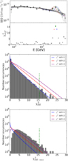 |
Fig. D.1. Results from the Monte Carlo simulations for the hypothesis of a narrow feature parameterized with an EP function with fixed curvature. First (top) panel: VHE gamma-ray spectrum from 2014 July 19 (MJD 56857.98), from Fig. 5, fitted with an LP function (thick dark gray curve), and also fitted with an LP plus an EP with β = 9.1, and centered at various energies from 0.08 TeV to 6.80 TeV in steps of 0.05 in base-10 logarithmic space (thin light gray lines). The difference in χ2 values ( |


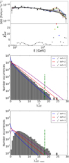 |
Fig. D.2. Same as in Fig. D.1, but for an EP with a variable curvature (i.e., β is left free to vary in the spectral fits) to parameterize the narrow spectral feature. See text in Appendix D for further details. |
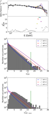 |
Fig. D.3. Same as in Fig. D.1, but for a Gaussian function with a variable width (i.e., sigma is left free to vary in the spectral fits) to parameterize the narrow spectral feature. See text in Appendix D for further details. |
Then, in the same way as for the Monte Carlo tests reported in Sect. 3.4, we use the LP function derived from the fit (thick dark gray curve in Figs. D.1–D.3) to generate 10 000 realizations of this spectrum with data points that have the same statistical uncertainty as the measured spectrum. We then performed a series of fits with a model composed of the baseline (LP) and the three cases for the narrow component: EP with fixed β, EP with variable β, and Gauss function with variable sigma. The parameter Ep for the EP function and mean for the Gauss function ranges from 0.08 TeV to 6.80 TeV in steps of 0.05 in log10 scale, as done before with the actual measured VHE spectrum. The distribution of  values obtained for the three distinct hypotheses are depicted in the second and third panels of Figs. D.1–D.3, and a summary of the resulting numbers are reported in Table D.1.
In Tombesi et al. (2010), only the highest  , namely
  , is considered. This number relates to the largest fluctuation (with the shape of the narrow feature) in the simulated spectrum. Here we also report the results obtained when using all the
  values obtained from the 40 × 10 000 spectral fits. When we consider the hypothesis of a narrow feature of fixed shape, which is the one resembling the test performed in Tombesi et al. (2010), and the most simple out of the three hypotheses investigated, the second panel of Fig. D.1 shows that the distribution of
  follows a χ2 with 1 degree of freedom. This is expected because, for each grid position, there is only one additional degree of freedom in the fit with the narrow component (the parameter K from the EP function); however, this shows that this test does not take into account that the location of the feature in the spectrum is arbitrary, and that a search in energy space is needed. When generating a large number of random tests, for a continuum spectrum where we make a search for additional components parameterized with two degrees of freedom (normalization and energy location), we would expect that distribution of
  to follow a nominal χ2 distribution with 2 degrees of freedom. On the other hand, the third panel of Fig. D.1 shows that the distribution of
  has a large deficit at low
  values, and is shifted to the right with respect to a nominal χ2 distribution for 2 degrees of freedom. This occurs by construction of the test because the cases with low
  values are systematically rejected. A similar situation occurs for the hypotheses where the shape of the narrow feature is not fixed, and hence an extra degree of freedom is added in the search (the curvature or width of the feature). The results for these tests are shown in Figs. D.2 and D.3, where the reference nominal χ2 distribution would be the one for 3 degrees of freedom.
We note that, when allowing for the curvature of the EP function to vary, the chance probability for a random fluctuation decreases slightly (see Table D.1). This is caused by the marginally better spectral fit to the measured VHE gamma-ray spectral points when using two degrees of freedom (see upper panels of Figs. D.1 and D.2):  increases from 15.6 to 18.1, which counteracts the larger freedom in the spectral fits to find narrow features in the simulated spectra. The numbers obtained with the EP and the Gaussian function with variable width are very similar because of the relatively large statistical uncertainties in the measured spectral data points: the results are dominated by the peak of the mathematical function used to describe the narrow spectral feature, and they are not affected by the tails of such function, which is where the Gauss and the EP function differ most.
Results from the Monte Carlo tests following the prescription from Tombesi et al. (2010), that are used to assess the chance probability (and related significance) of observing a spectral feature on top of the measured VHE gamma-ray spectrum described by an LP.
Appendix E: Characterization of the radio-optical emission with another SSC component
In this section we model the radio to optical UV emission for one of the nights of the sample (see Fig. E.1). For this model a simple PL electron distribution was used instead of the broken PL. The parameters used for this modeling are γmin = 1, γmax = 8 × 10⁴, n1 = n2 = 2.2, B = 0.02 [G], Density = 6 × 10³ [cm−3], R = 4.7 × 10¹⁶ [cm], δ = 10. With this approach the radio to optical emission could be fitted.
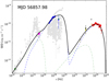 |
Fig. E.1. Broadband SED from 2014 July 21 (MJD 56859.97) where a two-zone SSC model has been used to describe the overall emission. One emitting region is responsible for the gamma-ray, X-ray and partially optical emission (dashed blue line). A second component explains the radio emission together with some optical emission (dashed green line). The colored spectral points represent the data sample from 56859.97. The gray spectral points represent the archival spectral points taken from the SED builder at SSDC. The peak emission at ∼1014−1015 Hz is due to the host galaxy contribution, which is not taken into account in our SSC model of the jet emission. |
Appendix F: Relation between γb and B
In the canonical one-zone SSC framework, we expect a break in the electron energy distribution, where the spectral indices change by one unit. This break occurs at the energy at which the timescale for energy loss is equal to the dynamical timescale. Given that the synchrotron bump and the inverse-Compton bump appear quite similar in the Mrk 501 SEDs from July 2014 (see Fig. 7), we can assume that the electrons lose energy roughly equally through synchrotron and inverse-Compton emission. In this case, the theoretical expectation for the location of the break would be given by the relation
where me is the electron mass, σT the Thompson cross section, and R the radius of the emitting region. Figure F.1 shows the evolution of γb as a function of B for the theoretical exercise reported in Sect. 4. The values used to parameterize the broadband SEDs agree typically within a factor of ∼2 with the theoretical expectations. Given that the one-zone SSC is a relatively simple theoretical scenario (e.g., the emission region may not be perfectly spherical and homogeneous), these differences between the employed values and the theoretical expectations in the canonical one-zone SSC can be considered in reasonable agreement.
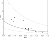 |
Fig. F.1. Evolution of the γb as a function of the magnetic field B for the one-zone SSC model reported in Sect. 4. The solid line represents the theoretical expectation assuming that γb is due to synchrotron and IC cooling (see Eq. (F.1)). The dotted lines depict the region with the energy break located a factor of 3 higher and a 50% lower than the theoretical expectation. |
All Tables
Summary of the Mrk 501 VHE observations performed with the MAGIC telescopes during the flaring activity that occurred in July 2014.
Results from the forward-folding fits with three different functions (PL, LP, and ELP) to the MAGIC VHE spectra observed and EBL-corrected (using the EBL model from Domínguez et al. 2011) from 2014 July 19 (MJD 56857.98).
Results from the forward-folding fits with an LP and an LP+EP to the MAGIC VHE spectra observed and EBL-corrected (using the EBL model from Domínguez et al. 2011) from 2014 July 19 (MJD 56857.98).
Results from the Monte Carlo tests used to quantify the chance probability (and related significance) of observing a spectral feature (parameterized with an LP+EP function) on top of the measured VHE gamma-ray spectrum described by an LP.
Spectral parameters for the Swift/XRT data from Mrk 501 in the energy range 0.3–10 keV during the high activity in July 2014.
Swit-BAT results from the analysis of Mrk 501 in the energy band 14–195 keV for one-day integration bins.
Spectral parameters for the MAGIC data from Mrk 501 in the energy range 0.1–10 TeV during the high activity in July 2014.
Results from the forward-folding fits with an LP up to 1.5 TeV to the single-night MAGIC VHE spectra that contains at least three spectral points beyond 1.5 TeV.
Results from the Monte Carlo tests following the prescription from Tombesi et al. (2010), that are used to assess the chance probability (and related significance) of observing a spectral feature on top of the measured VHE gamma-ray spectrum described by an LP.
All Figures
|
Fig. 1. Multi-wavelength light curve for Mrk 501 during the highest X-ray activity measured with Swift/XRT to date. The correspondence between the instruments and the measured quantities is given in the legends. The horizontal dashed lines in the VHE light curves depict the flux of the Crab nebula reported in Aleksić et al. (2016b). For BAT, the daily fluxes were computed using the spectral shape from the time interval MJD 56854.5–MJD 56872.5 (see Sect. 2.4.1). |
| In the text | |
|
Fig. 2. Fractional variability Fvar as a function of frequency. |
| In the text | |
|
Fig. 3. VHE flux in two energy bands (0.15–1 TeV and > 1 TeV) as a function of the Swift/XRT flux in two energy bands (0.3–2 keV and 2–10 keV). |
| In the text | |
|
Fig. 4. VHE SEDs from the MAGIC telescopes during the highest X-ray flux measured with Swift/XRT. Top and middle panels: black circles represent the observed SED from 2014 July 19 (MJD 56857.98), while the blue squares denote the same spectrum corrected for EBL absorption (using the model from Domínguez et al. 2011). In both panels the dotted lines depict the best LP fits (reported in Table 3), while the dashed lines show the best fits using data up to 1.5 TeV, and extrapolated beyond that energy (from the test reported in Table C.1). Bottom panel: VHE SEDs after EBL correction during three consecutive nights around 2014 July 19 (MJD 56857.98). |
| In the text | |
|
Fig. 5. VHE SED from 2014 July 19 (MJD 56857.98) measured with the MAGIC telescopes with an analysis that uses 25% more bins in estimated energy with respect to that shown in Fig. 4. Black circles represent the observed SED, while the blue squares denote the same spectrum corrected for EBL absorption (using the model from Domínguez et al. 2011). In both panels the dotted lines depict fits with an LP function, while the solid lines depict the fits with an LP+EP function. The parameter values resulting from the spectral fits are reported in Table 4. |
| In the text | |
|
Fig. 6. Distributions of |
| In the text | |
|
Fig. 7. Single-night broadband SEDs described with a one-zone SSC model. The VHE gamma-ray spectra from MAGIC are represented by the red dots, the Fermi-LAT spectra by the black (4 days) and yellow (10 days) triangles, the BAT emission by the blue triangles (using the spectral shape from XRT) and green triangles (using the spectral shape from the stacked BAT analysis over the time interval MJD 56854.5–MJD 56872.5), the binned X-ray spectra from XRT by the blue circles, the optical-UV observations from KVA and UVOT by the pink squares, and the radio observations from Metsähovi by the green squares. Most of the data samples were selected from observations taken within 3 h of each other. For MJD 56861 and MJD 56863 there were no Swift observations taken within the same night of the MAGIC observations, and we depicted the spectra (UVOT, XRT, and BAT) from the night before and the night after with gray symbols. Upper limits are shown as open symbols. See text in Sect. 4 for further details. |
| In the text | |
|
Fig. 7. continued. |
| In the text | |
|
Fig. 8. Broadband SED from 2014 July 19 (MJD 56857.98) modeled assuming a pileup in the electron distribution due to stochastic acceleration, and using two different values of the magnetic field: slow cooling with B = 0.1 G and fast cooling with B = 0.3 G. The color-coding for the data points is the same as in Fig. 7. See text in Sect. 5.1 for further details. |
| In the text | |
|
Fig. 9. Broadband SED from 2014 July 19 (MJD 56857.98) described with a two-zone SSC model that assumes co-spatial (left panel) and non co-spatial (right panel) locations of the emitting regions within the jet. For both panels, the emission from the small region (with narrow EED) is denoted by the red dot-dashed line, while the sum of the emission from the two regions is depicted by the black solid line. The color-coding for the data points is the same as in Fig. 7. See text in Sect. 5.2 for further details. |
| In the text | |
|
Fig. 10. Broadband SED from 2014 July 19 (MJD 56857.98) modeled with one-zone SSC emission (gray dashed and gray dot-dashed lines) and the emission from an IC pair cascade (red dot-dashed line). The sum of the two components is depicted by the black solid line. The color-coding for the data points is the same as in Fig. 7. See text in Sect. 5.3 for further details. |
| In the text | |
|
Fig. B.1. PL spectral index as a function of the integral flux, as observed by MAGIC in the energy bands 0.15–1 TeV and >1 TeV. |
| In the text | |
|
Fig. B.2. PL spectral index as a function of the integral flux, as observed by XRT in the energy bands from 0.3−2 keV and 2−10 keV. |
| In the text | |
|
Fig. D.1. Results from the Monte Carlo simulations for the hypothesis of a narrow feature parameterized with an EP function with fixed curvature. First (top) panel: VHE gamma-ray spectrum from 2014 July 19 (MJD 56857.98), from Fig. 5, fitted with an LP function (thick dark gray curve), and also fitted with an LP plus an EP with β = 9.1, and centered at various energies from 0.08 TeV to 6.80 TeV in steps of 0.05 in base-10 logarithmic space (thin light gray lines). The difference in χ2 values ( |
| In the text | |
|
Fig. D.2. Same as in Fig. D.1, but for an EP with a variable curvature (i.e., β is left free to vary in the spectral fits) to parameterize the narrow spectral feature. See text in Appendix D for further details. |
| In the text | |
|
Fig. D.3. Same as in Fig. D.1, but for a Gaussian function with a variable width (i.e., sigma is left free to vary in the spectral fits) to parameterize the narrow spectral feature. See text in Appendix D for further details. |
| In the text | |
|
Fig. E.1. Broadband SED from 2014 July 21 (MJD 56859.97) where a two-zone SSC model has been used to describe the overall emission. One emitting region is responsible for the gamma-ray, X-ray and partially optical emission (dashed blue line). A second component explains the radio emission together with some optical emission (dashed green line). The colored spectral points represent the data sample from 56859.97. The gray spectral points represent the archival spectral points taken from the SED builder at SSDC. The peak emission at ∼1014−1015 Hz is due to the host galaxy contribution, which is not taken into account in our SSC model of the jet emission. |
| In the text | |
|
Fig. F.1. Evolution of the γb as a function of the magnetic field B for the one-zone SSC model reported in Sect. 4. The solid line represents the theoretical expectation assuming that γb is due to synchrotron and IC cooling (see Eq. (F.1)). The dotted lines depict the region with the energy break located a factor of 3 higher and a 50% lower than the theoretical expectation. |
| In the text | |
Current usage metrics show cumulative count of Article Views (full-text article views including HTML views, PDF and ePub downloads, according to the available data) and Abstracts Views on Vision4Press platform.
Data correspond to usage on the plateform after 2015. The current usage metrics is available 48-96 hours after online publication and is updated daily on week days.
Initial download of the metrics may take a while.