| Issue |
A&A
Volume 634, February 2020
|
|
|---|---|---|
| Article Number | A54 | |
| Number of page(s) | 16 | |
| Section | The Sun | |
| DOI | https://doi.org/10.1051/0004-6361/201935872 | |
| Published online | 06 February 2020 | |
Spectroscopic detection of coronal plasma flows in loops undergoing thermal non-equilibrium cycles⋆
1
Institut d’Astrophysique Spatiale, CNRS, Univ. Paris-Sud, Université Paris-Saclay, Bât. 121, 91405 Orsay Cedex, France
e-mail: This email address is being protected from spambots. You need JavaScript enabled to view it.
2
Rosseland Centre for Solar Physics, University of Oslo, PO Box 1029, Blindern 0315, Oslo, Norway
3
Institute of Theoretical Astrophysics, University of Oslo, PO Box 1029, Blindern 0315, Oslo, Norway
4
Institute of Applied Computing & Community Code, Universitat de les Illes Balears, 07122 Palma de Mallorca, Spain
Received:
12
May
2019
Accepted:
5
December
2019
Abstract
Context. Long-period intensity pulsations were recently detected in the EUV emission of coronal loops and attributed to cycles of plasma evaporation and condensation driven by thermal non-equilibrium (TNE). Numerical simulations that reproduce this phenomenon also predict the formation of periodic flows of plasma at coronal temperatures along some of the pulsating loops.
Aims. We aim to detect these predicted flows of coronal-temperature plasma in pulsating loops.
Methods. We used time series of spatially resolved spectra from the EUV imaging spectrometer (EIS) onboard Hinode and tracked the evolution of the Doppler velocity in loops in which intensity pulsations have previously been detected in images of SDO/AIA.
Results. We measured signatures of flows that are compatible with the simulations but only for a fraction of the observed events. We demonstrate that this low detection rate can be explained by line of sight ambiguities combined with instrumental limitations, such as low signal-to-noise ratio or insufficient cadence.
Key words: Sun: corona / Sun: oscillations / Sun: UV radiation / techniques: spectroscopic
Movies associated to Figs. 1, 4, 7, 10 are available at https://www.aanda.org
Present address: Centre for mathematical Plasma Astrophysics, Department of Mathematics, KU Leuven, Celestijnenlaan 200B bus 2400, 3001 Leuven, Belgium.
© G. Pelouze et al. 2020
 Open Access article, published by EDP Sciences, under the terms of the Creative Commons Attribution License (http://creativecommons.org/licenses/by/4.0), which permits unrestricted use, distribution, and reproduction in any medium, provided the original work is properly cited.
1. Introduction
Understanding the energy transport and heating mechanisms that are capable of maintaining a million-degree corona around the Sun has been a long-standing challenge in astrophysics. Additional observational constraints are needed to identify the characteristics of heating processes (such as where it is localized and how it changes over time) and to discern different heating models. Long-period intensity pulsations in the extreme-ultraviolet (EUV) emission of coronal loops provide new observables that help constrain the parameters of the heating process. These pulsations were first detected by Auchère et al. (2014) based on images from the 195 Å channel of the Extreme-ultraviolet Imaging Telescope (EIT; Delaboudinière et al. 1995) onboard the Solar and Heliospheric Observatory (SOHO; Domingo et al. 1995) and by Froment et al. (2015) in images from the six coronal channels of the Atmospheric Imaging Assembly (AIA; Lemen et al. 2012) onboard the Solar Dynamics Observatory (SDO; Pesnell et al. 2012). The pulsations were reported to have periods ranging from 2 h to 16 h, with half of the events occurring in active regions and 25% being visually associated with loops (Auchère et al. 2014; Froment 2016).
These pulsations have been interpreted as the result of thermal non-equilibrium (TNE; Auchère et al. 2014, 2016; Froment et al. 2015, 2017, 2018) which can come from a quasi-constant heating localized near the loops footpoints. In this case, there may be no equilibrium between the heating near the footpoints and the radiative losses in the corona (Antiochos & Klimchuk 1991; Antiochos et al. 1999, 2000; Karpen et al. 2001; Klimchuk & Luna 2019; Antolin 2019; Klimchuk 2019). As a result, the plasma in the loop undergoes condensation and evaporation cycles (or TNE cycles) during which it periodically changes between a hot, tenuous phase and a colder, denser phase (Kuin & Martens 1982; Martens & Kuin 1983). Enhanced emission in the coronal channels of EIT or AIA occurs during cycles in which the plasma reaches a peak temperature of a few million degrees. This behavior is aptly reproduced in one-dimensional hydrodynamic simulations which compute the response of the plasma in a loop to a given heating function (Kuin & Martens 1982; Martens & Kuin 1983; Karpen et al. 2001, 2005; Müller et al. 2003, 2004, 2005; Antolin et al. 2010; Xia et al. 2011; Mikić et al. 2013; Mok et al. 2016; Froment et al. 2017, 2018). In particular, Froment et al. (2017) have been able to convincingly reproduce the intensity and emission measure from one of the events observed with AIA that they presented in their previous paper (Froment et al. 2015).
Periodic plasma flows naturally occur in the loop during a cycle, with upflows of hot plasma in both legs during the evaporation phase (simulations of case 1 of Froment et al. 2017 predict ∼10 km s−1) and strong downflows of cooling plasma that moves towards one of the footpoints during the condensation phase (simulations predict ≳50 km s−1 along the loop for plasma at coronal temperatures). The evaporation phase happens during the minimum of density, which results in very low emission in all the coronal channels of AIA. Therefore, we expect that the upflows will be harder to detect. The downflows start with plasma at coronal temperatures. Depending on the heating parameters, this plasma may then cool down to chromospheric temperatures and form periodic coronal rain showers, or it may be reheated early, thus remaining at coronal temperatures throughout the cycle.
Coronal rain has long been observed in chromospheric and transition region spectral lines, forming blob-like structures which appear to fall along coronal loops (Kawaguchi 1970; Leroy 1972; Foukal 1978; Schrijver 2001; De Groof et al. 2004, 2005; O’Shea et al. 2007; Antolin et al. 2010; Antolin & Rouppe van der Voort 2012; Vashalomidze et al. 2015). The formation and dynamics of coronal rain is reproduced with simulations of TNE, both in 1D simulations mentioned above, in 2.5D (Fang et al. 2013, 2015) and in 3D (Moschou et al. 2015; Xia et al. 2017). Coronal rain may also be observed in post-flare loops, where the plasma evaporates and catastrophically cools as a result of the intense transient heating from the flare (Scullion et al. 2016). Despite the large number of observations of coronal rain, the periodic nature predicted by simulations of TNE has only been observed recently by Auchère et al. (2018). The authors report the detection of periodic coronal rain showers observed off-limb in the 304 Å channel of AIA.
In this paper, we attempt to detect the flows of plasma at coronal temperatures, which occur regardless of whether coronal rain forms later during the cycle. While coronal rain is better observed off-limb where it forms distinct blobs (De Groof et al. 2004, 2005; Antolin & Rouppe van der Voort 2012), plasma at coronal temperatures has less distinct structures that could be tracked in plane-of-the-sky images. Therefore, we attempted to detect these flows on the disk by measuring the Doppler velocity using spectroscopic data from the EUV Imaging Spectrometer (EIS; Culhane et al. 2007) onboard Hinode (Kosugi et al. 2007), which can observe lines formed at coronal temperatures. Depending on the exposure time, EIS can measure velocities with an accuracy ranging from 0.5 to 5 km s−1 (Culhane et al. 2007; Mariska et al. 2008).
A number of observational studies have reported average velocities of a few km s−1 in both active regions and the quiet Sun. Transition region lines show systematic redshifts, while coronal lines show blueshifts (Sandlin et al. 1977; Peter & Judge 1999; Teriaca et al. 1999; Dadashi et al. 2011). While this may change the absolute Doppler velocities in coronal loops, it should not affect the amplitude of the velocity variations. Furthermore, evidence of flows associated with condensation in loops have been reported both at transition-region and coronal temperatures (O’Shea et al. 2007; Kamio et al. 2011b; Orange et al. 2013). However, the periodic nature of the flows at coronal temperatures has never been observed.
To get an estimation of the expected velocity variations, we look at a simulation of TNE cycles without the formation of coronal rain, which was performed by Froment et al. (2017) using the realistic geometry from a loop in which Froment et al. (2015) detected long-period intensity pulsations. In this simulation, the velocity along the loop leg changes from −10 to +55 km s−1 over a cycle, hence an amplitude of 65 km s−1. Simulations of coronal rain formed during TNE cycles predict velocities as high as several 100 km s−1 (Müller et al. 2004; Antolin et al. 2010; Johnston et al. 2019). However, these fast flows only occur when the plasma reaches transition-region or chromospheric temperatures and should, therefore, not be observed in coronal-temperature lines. Simulations from Froment et al. (2018) show that the velocity profiles are similar for cycles both with and without coronal rain outside of the coronal rain phase, with values that are consistent with Froment et al. (2017). They further show that the coronal rain phase only occupies a few percent of the cycle period. Hence, cycles with and without coronal rain should have similar velocity signatures in spectral lines formed at coronal temperatures.
However, accurately predicting the Doppler velocity signature of such flows is challenging as it is affected by the projection and integration along the line of sight (LOS). The angle between tho loop and the LOS could be estimated using magnetic field extrapolation and loop tracing methods in EUV images (see, e.g., Warren et al. 2018 and references therein). The result would be different for every observed loop as it depends on the loop geometry and the LOS position. For the loop simulated by Froment et al. (2017), the velocity projected along the LOS of AIA or EIS changes from −5 to +30 km s−1 over a cycle in the loop leg.
Fully understanding the effects of LOS integration would require forward modeling from 2D or 3D simulations of TNE. How LOS integration affects the time lag signature of TNE cycles has been studied by Winebarger et al. (2016) using 3D simulations but no such work exists for the velocities. We approximate the effects of LOS integration by supposing that the plasma outside the loop is, on average, at rest. Using Monte-Carlo simulations (described in Sect. 5.1), we show that under this assumption, the Doppler velocity measured with EIS depends on the velocity along loop, the angle between the loop and the LOS and on the ratio of the intensities emitted by plasma in the loop (Iloop) and elsewhere on the LOS (ILOS). Simulations predict that the AIA 193 Å intensity (∼1.6 MK) emitted by a single loop strand can vary by a factor ranging from 10 (Winebarger et al. 2016, Fig. 6) to 100 (Froment et al. 2017, Fig. 11) during a TNE cycle. The coronal-temperature emission from the loop is, therefore, negligible at the intensity minimum of the cycle, such that Imin ≃ ILOS. Therefore, we can approximate Iloop/ILOS ≃ (Imax − Imin)/Imin. Taking into account the projection and integration along the line of sight, the measured Doppler velocity variations could range from about 3 to 30 km s−1. These velocities are comparable to the typical accuracy of EIS, and, therefore, they should be detectable.
We also take advantage of the EIS spectroscopic data to track the evolution of the density in some pulsating loops and compare it to the simulations.
In addition, multidimensional simulations by Fang et al. (2013, 2015) and Xia et al. (2017) predict that coronal rain should be accompanied by simultaneous counter-streaming flows occurring in adjacent field lines. If such flows occur at coronal temperatures, they should result in a periodic broadening of the spectral lines during the TNE cycles. However, the line width also depends on the temperature and the presence of downflows in the loop, which both change over a cycle. Separating these different contributions would require an extensive analysis which is outside of the scope of this paper.
In Sect. 2, we describe the search for sets of EIS data suitable for this analysis. In Sect. 3, we present the method used to analyze these datasets and to measure the velocity and density. In Sect. 4, we present the results from four datasets, two of which have velocities compatible with the simulations, despite being at the detection limit. We discuss these results in Sect. 5 and summarize them in Sect. 6.
2. Finding appropriate datasets
In order to detect the predicted pulsations in velocity, it is necessary to observe the same active region continuously during several pulsation periods, taking several measurements per period. For periods around 10 h, this translates to several days of observation. We used data from Hinode/EIS, which can acquire spatially resolved spectra (rasters) by scanning a slit across the field-of-view (FOV).
We considered 3181 long-period intensity pulsation events that were detected with AIA between 2010 and 2016 by Froment (2016) using the method presented in Froment et al. (2015). For each of these events, we systematically searched the EIS database1 for sets of rasters such that the:
-
FOV of each raster intersects with the region where pulsations are detected with AIA data;
-
FOV is wider than 55″ to exclude narrow rasters and sit-and-stare studies;
-
dataset duration is longer than three pulsation periods;
-
gaps between the rasters are neither too long nor too frequent (this last criterion is estimated qualitatively).
We did not constrain other raster parameters such as the exposure time, the slit width, or the step between consecutive slit positions.
Overall, 11 datasets were found. Their characteristics are presented in Table 1. In addition to the parameters of the EIS observations, this table shows the period of the intensity pulsations that were detected with AIA and an estimation of their amplitude during the EIS observing period. We quantify the amplitude of the pulsations with the contrast of the maximum to the minimum intensity ((Imax − Imin)/Imin), measured in the 193 Å band of AIA over a cycle. As argued in the introduction, this provides a reasonable approximation of the contrast between the loop and the background emission.
Main characteristics of the 11 EIS datasets that correspond to the observation of loops undergoing long-period intensity pulsations.
These datasets can be divided into three categories. The first and largest category (datasets 1–7) contains datasets with a good cadence (ten or more rasters per pulsation period), but with short exposure times (of less than 10 s) and, therefore, a low signal-to-noise-ratio (S/N). The second category (datasets 8 and 9) also contains datasets with a good cadence, composed of rasters that have longer exposure times (thus better S/N), but narrow FOVs (60″ along the X axis, i.e., perpendicular to the slit) and short total observing time (1.5 and 2.3 pulsation periods, respectively). Finally, the last category (datasets 10 and 11) contains rasters with the highest S/N, but with a very low cadence (about one raster per pulsation period). While none of these datasets fulfill all the criteria required to detect the expected pulsations with the utlmost certainty, those with both a good S/N and large-amplitude intensity pulsations should allow for the detection of the predicted velocities.
3. Analyzing time series of EIS rasters
We measured the intensity and Doppler velocity using the Fe XII 195.119 Å line. This line is formed at a temperature of 1.6 MK, which is attained during the cooling phase of most simulated cycles (Froment et al. 2017, 2018). It is also one of the brightest lines observed by EIS (Young et al. 2007), which helps maximize the S/N, as well as the main contributor to the AIA 193 Å band (Boerner et al. 2012), which allows for easy comparison with AIA observations. When the Fe XII 186.887 Å line is available, we derive the density from the Fe XII 186.887/195.119 Å ratio, which is sensitive to electron number density in the 1014 − 1018 m−3 range (Young et al. 2007, 2009) and covers the expected loop densities of 1014 − 1015 m−3 (Froment et al. 2017, 2018) for cycles where the plasma remains at coronal temperatures.
Data preparation and line fitting. Each EIS raster was first prepared into level 1 data using the eis_prep.pro routine from SolarSoft (Freeland & Handy 2012). We then fit gaussians to the Fe XII 195.119 Å and 186.887 Å lines using the SolarSoft routine eis_auto_fit.pro, which allows us to derive intensity and velocity maps for these two lines. The 195.119 Å line is blended with a weaker Fe XII line at 195.179 Å. We fit this feature using two gaussians that share the same width and have a fixed wavelength separation of 0.06 Å (Young et al. 2009). The wing of the 186.887 Å line contains a weaker line at 186.976 Å, which Brown et al. (2008) suggested could be a Ni XI transition. We used two independent gaussians to fit these lines. Fe XII 186.887 Å is also blended with a weak S XI line at 186.839 Å. Although the contribution from this line is difficult to quantify, Young et al. (2009) reported that it is below 10% and only has a small effect on the resulting densities. We decided, therefore, not to correct for its contribution. Each of the aforementioned electronic transitions results in two distinct contributions: a Doppler-shifted component from plasma flowing in the loop and a non-shifted component from plasma at rest elsewhere on the line of sight. We demonstrate in Sect. 5.1 that the velocity in the loop is best retrieved when fitting a single gaussian to each transition.
In addition, we verified whether the fit results were significantly altered when correcting for the effect described by Klimchuk et al. (2016), which is that the spectral intensity integrated within a wavelength bin is different from the intensity at the center of this bin. We tried to correct the spectral intensities using the Intensity Conserving Spectral Fitting method (Klimchuk et al. 2016). This marginally affected the fit results (typically 0.05 km s−1 for the line position, and 0.1% for the integrated intensity), hence, we did not correct the data for this effect.
Spatial coalignment. In order to get accurate pointing information, we coaligned all EIS rasters with AIA 193 Å images using the method presented in Pelouze et al. (2019). This allows for the correction of the pointing offset, the instrument roll, and the spacecraft jitter. All maps were then converted into Carrington heliographic coordinates in order to compensate for the effect of solar rotation. The differential rotation is corrected using the rotation rate Ω(ϕ) measured by Hortin (2003) for the 195 Å channel of EIT:
![Mathematical equation: $$ \begin{aligned} \Omega (\phi ) = 14.50 - 2.14 \sin ^2\phi + 0.66 \sin ^4\phi \ [^{\circ }\,\mathrm{day}^{-1}] \end{aligned} $$](/articles/aa/full_html/2020/02/aa35872-19/aa35872-19-eq1.gif) (1)
(1)
where ϕ is the heliographic latitude.
Velocity measurement. The velocity was derived from the centroid of the fitted Fe XII 195.119 Å line. We adopted the convention that positive velocities correspond to spectral redshifts, meaning plasma that is moving away from the observer.
Correction of orbital effects. The velocities measured with EIS are affected by thermoelastic deformations of the instrument caused by the orbit of Hinode: over the 98-min orbit, the position of the spectrum on the detector drifts periodically, which introduces time-dependant velocity variations of up to 70 km s−1 (Brown et al. 2007; Kamio et al. 2010, 2011a). The measured absolute velocities can therefore change significantly between different rasters, or even within a raster if the raster duration is comparable to the orbital period. Two different methods can be used to correct for this spectrum drift. In the first method, the quiet Sun is used as a reference to estimate the drift directly from the data (see, e.g., Brown et al. 2007; Mariska et al. 2007; Young et al. 2012). The second method was developed by Kamio et al. (2010) and uses an empirical model to predict the spectral drift from EIS housekeeping data. The Kamio et al. (2010) correction is applied within the SolarSoft routine eis_auto_fit.pro, but it does not fully correct for the spectral drift, leaving residuals of about 5 km s−1.
A second correction was, thus, needed to detect the pulsations of a few kilometers per second. The high cadence datasets (1–7) are composed of rasters with narrow FOVs (162″ × 152″ to 180″ × 152″) centered on the active region, which contain little to no quiet Sun. For these rasters, we used as a reference the Fe XII 195.119 Å velocity averaged in the region over which the FOVs of 95% of the rasters overlap, and set it to 0 km s−1. Because the duration of these rasters is short compared to the orbit (2.7–4.5 min vs. 98 min), it is acceptable to use a common velocity reference for all slit positions. The other datasets (8–11) have tall FOVs (368″ to 512″), which usually contain quiet Sun at the North or South of the active region. In this case, we computed the average velocity in the quiet Sun region for each slit position and used it as a reference. We corrected the intrinsic quiet Sun velocity using the method described by Young et al. (2012) and the average shift of −2.4 km s−1 reported by Dadashi et al. (2011) for Fe XII.
Density measurement. The density was measured through the Fe XII 186.887/195.119 Å lines ratio, which is sensitive to density variations in the 108 − 1012 cm−3 range (Young et al. 2007, 2009). We derived the densities from this line ratio using Chianti version 8 (Dere et al. 1997; Del Zanna et al. 2015) and assuming the temperature of 1.6 MK, the peak formation temperature of Fe XII. The density could not be measured in datasets 1, 4, 6, and 7 because they do not contain the Fe XII 186.887 Å line.
After applying the previous steps, we obtained time series of corrected intensity, velocity, and (when possible) density maps for each of the datasets listed in Table 1.
4. Results
We present the analysis of four of the datasets presented at the end of Sect. 2: datasets 1 and 8 for which the S/N and the amplitude of the intensity pulsations are large enough to allow for the detection of velocity variations that are compatible with the expected pulsations (Sect. 4.1); datasets 2 and 11 in which no velocity pulsations could be detected either due to a low S/N, or to insufficient cadence (Sect. 4.2). No pulsations in velocity were detected in the other datasets.
4.1. Datasets with velocities consistent with the expected pulsations
Dataset 1 corresponds to the observation of active region NOAA 11283, in which intensity pulsations with a period of 5.8 h were detected in the 211 Å channel of AIA, between 2011 September 2, 13:08 UT and September 8, 14:18 UT. The EIS dataset contains 240 rasters recorded between 2011 September 3, 10:56 UT and September 5, 02:56 UT, amounting to 40.1 h of observation. All rasters use the 2″ slit, 9 s of exposure time, a scan step of 6″, and have a FOV of 180″ × 152″. The FOV is shown in Fig. 1, which contains the intensity and velocity maps from raster eis_l0_20110903_105615 projected onto Carrington coordinates corrected for the differential rotation, as well as the region in which the intensity pulsations are detected with AIA. We select three regions of 1.8 ° ×1.8° in which we examine the evolution of the intensity and velocity: one close to the apex of the loop (green square), one at its eastern leg (red square), and one outside the pulsating loops (yellow square) that we use as a reference for the velocity. We verify that the specific shape, position, and size of the regions do not significantly modify the time series. While some pixels of the regions seem to be outside the loop, they do not reduce the amplitude of the intensity and velocity variations. The reference region is chosen such that it contains small velocity variations and no pulsations in the AIA 193 Å intensity (we verify that the power spectral density computed using the method presented in Auchère et al. 2014 contains no excess power in this region). These 1.8 ° ×1.8° on the solar sphere correspond to 30″ × 30″ in the plane of the sky for regions at the disk center. For dataset 1, this corresponds to 5 pixels in the solar-X direction and 30 pixels in the solar-Y direction, thus, 150 pixels in each region. Finally, we add a manually-traced contour that follows the shape of the loop as seen in the AIA 193 Å images.
 |
Fig. 1. Maps of the Fe XII 195.119 Å line emission (top) and velocity (bottom) for raster eis_l0_20110903_105615 from dataset 1, projected onto Carrington coordinates. This raster was acquired on 2011 September 3 between 10:56 UT and 11:01 UT. Several regions of interest are represented on the map: the contour in which intensity pulsations are detected with AIA 193 Å (blue), the contour selected for the loop leg (red), the contour selected for the loop apex (green), a reference contour outside the loop (yellow), and the shape of the underlying loop (light blue). The temporal evolution of AIA 193 Å can be seen in the online movie. |
In Fig. 2, we show the time series associated with dataset 1. The top panel (Fig. 2a) shows the intensities from the EIS Fe XII 195.119 Å line, from AIA 211 Å (the channel in which the intensity pulsations are detected), and from AIA 193 Å (which is dominated by the Fe XII 195.119 Å line; Boerner et al. 2012), averaged over the detection contour presented in Fig. 1. The two AIA channels display similar pulsations, with 193 Å peaking after 211 Å. There is a good match between the intensities from EIS Fe XII 195.119 Å and AIA 193 Å. The small deviations between the two could be caused by other contributions in the passband of AIA, or the fact that the FOV of EIS does not contain the full detection contour (see Fig. 1). We construct a time series of AIA 193 Å intensities sampled at the same locations as the EIS rasters, also shown in Fig. 2a. This better matches the EIS intensities, thus we conclude that the difference between the EIS and AIA intensities is mainly caused by sampling effects.
 |
Fig. 2. Time series of the intensity and velocity for dataset 1, averaged in the contours defined in Fig. 1. (a) Comparison of intensities in the detection contour: EIS Fe XII 195.119 Å ( |


The Fe XII 195.119 Å intensities averaged over the regions shown in Fig. 1 are presented in Fig. 2b. The time series are divided by their respective average values, which are given in the caption of Fig. 2. The intensity in the loop apex and leg have the same behavior as the intensity in the full detection contour. The intensity in the reference region shows some variations, but these are not always in phase with the variations of the pulsating loop.
The associated velocities are shown in Fig. 2c. We estimate the uncertainty on the velocity to ±0.4 km s−1 by computing the standard-deviation of the time series from the reference region, which contains no feature. This value is consistent with the usual ±5 km s−1 uncertainty for one EIS pixel (Culhane et al. 2007), divided by the square root of the number of EIS pixels in the region (150 pixels as previously stated), which gives an uncertainty of 0.41 km s−1.
Compared to the reference region, the velocities at the loop apex (green) and the loop leg (red) show more variance. Some fluctuations are in phase with the peaks of intensity. In particular, four peaks are visible in the loop leg at 3.5, 25.3, 30, and 38.5 h, which all happen at the same time as intensity peaks. These intensity and velocity peaks are indicated by black arrows on Fig. 2. The peaks at 3.5 and 25.3 h have an amplitude of about 3 km s−1. We argue that these are significant because they are above the uncertainty level, and are not present in the reference region. However, there are no features in velocity associated with the other strong intensity peak around 17 h.
Figure 3 shows the evolution of the AIA 193 Å intensity, the EIS Fe XII 195.119 Å intensity, and the velocity along the loop shape defined in Fig. 1 (s is the position along the loop starting at the eastern footpoint, and the measured parameters are averaged transversely over the loop width). Each row of the EIS intensity and velocity plots corresponds to a different raster. In this dataset, there are no data at the loop apex because it is not in the FOV of EIS. The intensity pulsations are visible along the loop in both AIA and EIS, except near the western footpoint where the emission appears to be dominated by another structure below or above the footpoint. This structure can be seen in the AIA movie (Fig. 1) and starts expanding near the western footpoint after 2010 November 4 00:00 UT. Six intensity peaks (marked by white arrows) are visible with EIS, at 0.5, 3.5, 16.5, 25.3, 30, and 38.5 h. Four of these peaks have associated downflows, visible at 3.5, 25.3, 30, and 38.5 h.
 |
Fig. 3. Evolution of the AIA 193 Å intensity (left), EIS Fe XII 195.119 Å intensity (middle), and velocity (right), as a function of the position along the loop shape of dataset 1 defined in Fig. 1, and of time. s = 0 corresponds to the eastern footpoint, and the values are averaged over the loop width. Each row of the EIS plots (middle and right) corresponds to a different raster of the dataset. The vertical lines show the limits of the AIA detection contour, and the arrows correspond to the peaks marked in Fig. 2. |
Dataset 8 corresponds to the observation of NOAA AR 11120, where 3.9-hour intensity pulsations were detected in the 171 Å channel of AIA, between 2010 November 2, 09:10 UT, and November 8, 01:27 UT. The EIS dataset contains 60 rasters that were recorded between 2010 November 3, 21:15 UT, and November 4, 02:58 UT. This corresponds to 5.8 h of observation, which is much shorter than dataset 1 and covers only 1.7 pulsation periods. The rasters use the 2″ slit, with 20 s of exposure time, a scan step of 4″, and have a FOV of 60″ × 368″. Only the western half of the pulsating loop is visible in this narrow FOV.
We performed the same analysis as on the previous dataset and we present similar figures: Fig. 4 shows the FOV of raster eis_l0_20101103_211534 and the selected regions; Fig. 5 shows the associated time series; and Fig. 6 shows the evolution of the intensity, velocity, and density along the loop. Given the 4″ scan step, each of the 1.8 ° ×1.8° regions shown on Fig. 4 corresponds to 225 pixels at disk center. The two channels of AIA show similar intensity pulsations, with 171 Å peaking after 193 Å. The difference between the AIA 193 Å and EIS Fe XII 195.119 Å intensities appears to be dominated by sampling effects, as in dataset 1. The narrow FOV of this dataset makes it difficult to find a reference region in which the intensity does not change much over time, while remaining high enough to allow for accurate velocity measurements. While the region that we select shows some intensity variations (Fig. 5b), it shows no velocity variations (Fig. 5c), which is the most important detail to estimate uncertainty on the velocity.
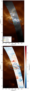 |
Fig. 4. Same as Fig. 1, but with the FOV of raster eis_l0_20101103_211534 from dataset 8, acquired on 2010 November 3 between 21:15 UT and 21:20 UT. Both maps are overlaid on a AIA 193 Å map to help visualize the structure of the active region. The temporal evolution of AIA 193 Å can be seen in the online movie. |
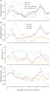 |
Fig. 5. Same as Fig. 2, but showing the parameters of dataset 8 averaged in the contours defined in Fig. 4. (a) EIS Fe XII 195.119 Å and AIA 193 Å intensities. (b) EIS Fe XII 195.119 Å intensity normalized to ( |


The velocity (Fig. 5c) has a very small variance in all contours. However, three small fluctuations are visible in the loop leg, with peaks at 0.7, 2.7, and 4.5 h. These are visible in both Figs. 5c and 6, and have an amplitude of less than 2 km s−1. We estimate the uncertainty on the velocity using the values from the reference region to ±0.6 km s−1. The observed variations are therefore significant, although very close to the detection limit. Two of these velocity peaks are associated with intensity maxima and separated by 3.5 h, that is, approximately one period. However, the peak at 2.7 h does not appear to be associated with any intensity feature.
 |
Fig. 6. Same as Fig. 3, but for dataset 8, showing the evolution of the AIA 193 Å intensity (top left), EIS Fe XII 195.119 Å intensity (top right), velocity (bottom left), and density (bottom right) in the loop represented in Fig. 4. |
Finally, we measure the density in this dataset and plot it in Figs. 5d and 6. Similarly to the intensity, the time series are normalized to their average values, which are specified in the caption. Small density fluctuations (∼20%) are measured in the selected contours, and are visible in Fig. 5d. Two maxima are observed in the leg (marked by black arrows), which coincide with the intensity peaks. A single peak is visible in the density at the apex, which happens about 0.2 h before the first density peak seen in the loop leg. The density peak at the apex is accompanied by co-temporal intensity and velocity peaks at the apex, visible in Fig. 5b and c. The density variations are also visible in Fig. 6, which shows the evolution of the density along the loop. The density in the other regions is not correlated with the variations in intensity.
4.2. Datasets with no pulsations because of instrumental limitations
Dataset 2 corresponds to the observation of NOAA AR 11494, in which pulsations were detected in the 193 and 335 Å channels of AIA between 2012 June 3 18:44 UT, and June 9 11:39 UT, with a period of 4.9 h. The EIS dataset contains 178 rasters recorded between 2012 June 8 03:03 UT and June 9 07:42 UT, amounting to 28.7 h of continuous observation. All rasters use the 2″ slit, a 3 s exposure time, a scan step of 3″, and have a FOV of 152″ × 162″. At this exposure time, the S/N is three times lower than in dataset 1 and seven times lower than in dataset 8.
We present similar figures as we have given for the previous dataset: the FOV of raster eis_l0_20120608_230140 and the regions of interest are shown in Fig. 7 (each region corresponds to 300 pixels at disk center). The associated time series are shown in Fig. 8, and the evolution of the intensity and velocity along the loop are shown in Fig. 9. For this dataset, the intensity in the loop leg seems to peak after the intensity at the apex (Fig. 8b). This is consistent with falling material at coronal temperatures, but such behavior is not observed in the other datasets. Contrary to datasets 1 and 8, there is no significant evolution of the velocity, which is most likely explained by the fact that the S/N is significantly lower in this dataset. Velocity variations can be seen in the western part of the loop in Fig. 9, but these are not correlated with the intensity peaks. However, a prominent peak is visible in the density around 16 h at the apex and around 17.5 h in the loop leg (Fig. 8d). This falls between two intensity peaks at 11 and 20 h.
 |
Fig. 7. Same as Fig. 1, but with the FOV of raster eis_l0_20120608_230140 from dataset 2, acquired on 2012 June 8 between 23:01 UT and 23:05 UT. The temporal evolution of AIA 193 Å can be seen in the online movie. |
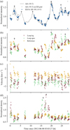 |
Fig. 8. Same as Fig. 2, but showing the parameters of dataset 2 averaged in the contours defined in Fig. 7. (a) EIS Fe XII 195.119 Å and AIA 193 Å intensities. (b) EIS Fe XII 195.119 Å intensity normalized to ( |


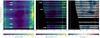 |
Fig. 9. Same as Fig. 3, but for dataset 2, showing the evolution of the intensity and velocity in the loop represented in Fig. 7. |
Dataset 11 corresponds to the observation of AR NOAA 12135 in which pulsations were detected in the 193 Å channel of AIA, between 2014 August 9 10:56 UT, and August 15 12:26 UT, with a period of 5.8 h. The dataset contains 21 rasters acquired between 2014 August 9 15:37 UT and August 14 11:41 UT, amounting to 116.8 h of observation with a very low cadence of one raster every 5.6 h on average. It is composed of two kinds of rasters: the first uses study HPW022_VEL_480x512v1 (ID: 480), with an exposure time of 15 s, and a wide FOV of 480″ × 512″; the second kind uses the EIS study HPW021_VEL_120x512v2 (ID: 428), with an exposure time of 45 s, and a relatively narrow FOV of 120″ × 512″. All rasters use the 1″ slit.
Figure 10 shows the intensity and velocity maps of raster eis_l0_20140810_042212 (wide FOV), the contour of raster eis_l0_20140810_192924 (narrow FOV), the region in which the intensity pulsations are detected in AIA, and a loop shape that extends this detection contour towards the footpoints. The eastern part of the loop is covered by both raster types, while the western part is only seen in rasters with a wide FOV. Figure 11 shows the evolution of the intensity in the detection contour. The 5.8-hour pulsations are clearly visible in the AIA 193 Å time series, and the EIS Fe XII 195.119 Å intensity matches its evolution. However, the cadence of the EIS rasters is not high enough to detect the pulsations with these data only. Figure 12 shows the evolution of the intensity and velocity along the loop contour defined in Fig. 10. Despite a good S/N that allows for accurate velocity measurements, no velocity nor intensity pulsations can be seen in the EIS plots. However, downflows are detected in the western part of the loop (0.6 < s < 0.9), while the eastern legs contains either upflows or no velocities. This is compatible with either a static flow along the loop, or the expected pulsations, but the cadence does not allow us to discriminate between the two scenarios.
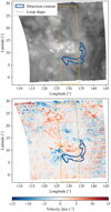 |
Fig. 10. Same as Fig. 1, but with the FOV of raster eis_l0_20140810_042212 from dataset 11, acquired on 2014 August 10 between 04:22 UT and 05:29 UT. The AIA detection contour is shown in dark blue, the loop shape in light blue, and the FOV of raster eis_l0_20140810_192924 is shown in yellow. The temporal evolution of AIA 193 Å can be seen in the online movie. |
 |
Fig. 11. Intensity evolution for dataset 11, averaged in the detection contour shown in Fig. 10: AIA 193 Å at full resolution ( |


 |
Fig. 12. Same as Fig. 3, but for dataset 11, showing the evolution of the intensity and velocity in the loop represented in Fig. 10. |
5. Discussion
5.1. Magnitude of the measured downflows
The one-dimensional hydrodynamic simulations of loops that reproduce the observed long-period intensity pulsations also predict periodic plasma flows, where the velocity along the loop changes over one cycle with an amplitude of about 60 km s−1 (Mikić et al. 2013; Froment et al. 2017, 2018). Such variations in velocity should be easy to detect with Hinode/EIS, which can measure velocities with a precision of about 5 km s−1 in a single pixel (Culhane et al. 2007). We searched for such pulsations by analyzing 11 EIS datasets, nine of which had sufficient cadence to allow for the detection of pulsations. Yet we did not detect velocity pulsations with the expected amplitude in any of these datasets. Instead of this, we detect velocity variations with an amplitude of 2–4 km s−1 in two datasets, which are the ones that have the highest S/N, and the most contrasted intensity variations. The measured velocity variations are therefore lower by at least a factor of 10 than those produced in the simulations.
This apparent discrepancy is caused by the fact that coronal loops are only 10–30% brighter than the background when observed in EUV (Del Zanna & Mason 2003; Aschwanden & Nightingale 2005; Aschwanden et al. 2008) and, therefore, only contribute to a small fraction of the emission integrated over the full line of sight (LOS). Let’s consider a LOS filled with plasma at rest, that intersects at an unknown angle θ with a single loop inside which plasma flows at a velocity vloop, as illustrated in Fig. 13. In this situation, the velocity projected on the LOS is vloop cos θ, and a given electronic transition with an energy equivalent to the rest wavelength λ0 (Fe XII 195.119 Å in our case) would result in two distinct contributions: a bright contribution centered on λ0 emitted by everything outside the loop and a dimmer contribution emitted by the plasma flowing in the loop, centered on (vloop cos θ/c + 1)λ0 and only 10–30% as bright as the first line. Because of the combined Doppler broadening and instrumental width, line profiles observed by EIS have typical full widths at half-maximum (FWHM) of 60 mÅ, or 95 km s−1 (Korendyke et al. 2006; Brown et al. 2008). With an expected separation of cos θ × 60 km s−1, the two lines are, therefore, blended, and retrieving the velocity of the fainter component is not straightforward. This may be achieved by fitting the two lines with either a single or two Gaussian profiles.
 |
Fig. 13. Sketch representing the integration along the LOS of a spectral line emitted by plasma flowing in a loop (red), and the contribution from static plasma in the background and foreground (yellow). Even if the component from the loop has an important spectral shift, the resulting line (dashed blue) is close to the rest wavelength, because the loop accounts only for 10–30% of the total emission. |
We tested these two approaches by performing Monte-Carlo simulations, in which we generate synthetic spectra similar to the one described above (i.e., two gaussian profiles at positions vrest = 0 and vloop cos θ > 0, intensities Irest > Iloop, and a common FWHM Δ), add photon noise, and fit the spectra with either one or two Gaussian profiles. By repeating this operation a large number of times for different realizations of the noise, we can estimate the probability of correctly retrieving the input parameters. We explore different values for the wavelength separation, intensity ratio, and S/N of the two lines. This is detailed in Appendix A. We draw two conclusions from these simulations: (1) given the S/N of the EIS observations, the velocity of the second component cannot be estimated with a two-gaussians fit because the locations of the two fitting Gaussians are decorrelated from the input for vloop lower than 80 km s−1 or 150 km s−1 depending on the S/N (Fig. A.2); (2) when performing a single-gaussian fit, the retrieved velocity vFit is systematically lower than the one in the loop (Fig. A.1), with:
 (2)
(2)
These simulations justify the use of a single-gaussian fit to retrieve the velocity of a faint component with a small wavelength separation and provide a new way to interpret the fit results. Double gaussian fitting is, therefore, more suited to larger separations (see, e.g., Imada et al. 2008; Dolla & Zhukov 2011 who applied this method to retrieve separations of 50–100 km s−1 from EIS spectra), while the B–R asymmetry index (De Pontieu et al. 2009) is adapted to more complex line profiles, but do not allow for straightforward velocity measurements.
We use the intensity contrast presented in Table 1 as an estimation of Iloop/Irest to compute a lower bound to the amplitude of the velocity variations in the loops using the above Eq. (2): vloop, min cos θ = vFit × Irest/Iloop. In dataset 1, we measured variations of 3.0 ± 0.4 km s−1 and an intensity contrast of 50%, which translates to vloop, min cos θ = 6 km s−1. For dataset 8, the measured variations are of 2.0 ± 0.6 km s−1 with a contrast of 20%, which gives vloop, min cos θ = 10 km s−1. These values are closer, although still lower, to those produced in the simulations. Part of this difference results from the projection of the LOS. In the case of dataset 1, the measured velocity could be further reduced by the orbital drift correction, for which we used the velocity averaged over the FOV (Sect. 3). The reference region used to correct the orbital drift therefore includes the pulsating loops, which could slightly attenuate the velocity variations. The presence of counter-streaming flows (Fang et al. 2013, 2015; Xia et al. 2017) may further explain the small velocity variations. Such flows would indeed add a blueshifted contribution to the spectral line, which would shift its centroid towards lower velocities. However, the current analysis does not allow us to observe whether such flows are present in the loops.
Finally, the LOS integration effect can also explain why pulsations are not seen in all datasets: in most datasets, the measured velocity would be reduced by the background and foreground to the point that it falls below the detection threshold of EIS. Datasets 1 and 8, where velocity variations are measured, are the ones with the most favorable combination of S/N and intensity contrast.
5.2. Time shifts between intensity, velocity, and density
We then investigated how the intensity, velocity, and density signals are shifted relatively to each other, as it is a signature of TNE. In datasets 1 and 8, almost all observed velocity peaks happen at the same time as the Fe XII 195.119 Å intensity peaks. The density peaks are less consistent: it appears to be in phase with the intensity in dataset 8, while it is in opposition of phase in dataset 2.
In order to better understand these behaviors, we took a new look at simulation results from Froment et al. (2017), which reproduced the intensity pulsations observed with AIA for one of the events presented by Froment et al. (2015). This simulation was performed by Froment et al. (2017), who used the method described by Mikić et al. (2013) to compute the hydrodynamic evolution of the plasma along a fixed magnetic field line with a non-uniform area expansion. Although this simulation was performed for a different event than the ones presented in the current study, we use it to get a global idea of the evolution of a loop undergoing TNE cycles. In Fig. 14 (adapted from Fig. 9 of Froment et al. 2017), we present the evolution of the AIA 193 Å intensity, temperature, density, and velocity (along the loop and projected along the LOS of AIA or EIS), averaged at the loop apex (top) and in the western leg of the loop (bottom), which is the leg towards which the condensations fall. We first note that the velocity in the western leg peaks to 55 km s−1 along the loop, which corresponds to only 30 km s−1 when projected along the LOS of AIA or EIS, as mentioned in Sect. 1. In the eastern leg (not shown in Fig. 14), the velocity only reaches 15 km s−1 along the loop, which is even smaller than the velocity at the apex. This is not surprising given that the condensations do not flow towards this leg. At the apex, the density peaks before the intensity, while the velocity peaks roughly at the same time as the intensity. In the loop leg, however, all parameters peak approximately at the same time. Therefore, we expect the velocity to be in phase with the intensity everywhere in the loop, but the density should peak at the loop apex before peaking in the leg.
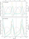 |
Fig. 14. Synthetic AIA 193 Å intensity I193, temperature Te, density Ne, and velocity (vloop along the loop, and vLOS projected along the line of sight), in the loop simulated by Froment et al. (2017), and adapted from Fig. 9 of their paper. Top: values near the apex, averaged between 170 and 255 Mm of the 367 Mm-long-loop. Bottom: values in the loop leg, averaged between 320 and 340 Mm. The intensity, temperature, and density are divided by their standard deviation and shifted by their average. Ne peaks before I193, vloop, and vLOS at the apex, but all peak roughly at the same time in the leg of the loop. |
In dataset 8, two density peaks occur in the leg at the same time as the two intensity peaks, around 0.7 and 4.5 h (Fig. 5). One density peak is visible at the apex at 0.5 h, just before the first peak that occurs in the leg at 0.7 h. The time shifts of these three density peaks is consistent with the simulations. However, the second density peak is not visible at the apex (this could be due to no variations or insufficient contrast), and we cannot fully test the fact that the density should peak before the intensity at this location. A single but prominent density peak is detected in dataset 2, which arises first at the apex at 16 h, and then in the leg at 17.5 h (Fig. 8). Although the density in the leg does not peak at the same time as the intensity, the fact that it peaks after the apex seems compatible with the simulations.
The velocities measured in datasets 1 and 8 are globally consistent with the predicted behavior. Indeed, the downflows observed in dataset 1 all happen at the same time as the Fe XII 195.119 Å intensity peaks, and all intensity peaks have associated downflows, except for the strong intensity peak at 17 h. In dataset 8, the two intensity peaks have associated downflows. However, a third velocity peaks is seen at 2.7 h, and does not appear to be associated with any intensity feature, which is puzzling. Overall, the fact that most downflows happen at the same time as the corresponding intensity peaks is a strong clue that they are not instrumental artifacts.
Finally, we note that the AIA 211 Å intensity peaks before 193 Å in dataset 1 and that 193 Å peaks before 171 Å in dataset 2. This is consistent with previous reports that loops (undergoing TNE or not) are generally observed in their cooling phase (Warren et al. 2002; Winebarger et al. 2003; Winebarger & Warren 2005; Ugarte-Urra et al. 2006, 2009; Mulu-Moore et al. 2011; Viall & Klimchuk 2011, 2012; Froment et al. 2015).
6. Summary and conclusion
In order to detect velocity pulsations associated with long-period intensity pulsations, we used 11 sets of EIS rasters that correspond to the observation of known intensity pulsation events detected with AIA between 2010 and 2016 (Froment 2016). We detected velocity variations compatible with the expected pulsations in two of these datasets. The variations are characterized by recurring downflows that happen at the same time as the intensity peaks. The first dataset (1) contains six intensity peaks, four of which have matching velocity peaks. The second dataset (8) contains two intensity peaks but shows three velocity peaks, with the third one occurring between the two intensity peaks. Overall, we find a good, albeit not perfect, correlation between the observed intensity and velocity peaks for these two datasets. The observed velocities are consistent with simulations from Mikić et al. (2013) and Froment et al. (2017), where strong downflows occur in one leg of the loop when the intensity peaks in the 193 Å channel of AIA. Note that such velocity signature can correspond to condensation and evaporation cycles with or without formation of coronal rain. The velocity variations have an amplitude of 4 and 2.5 km s−1, respectively, which is much lower than the ∼30 km s−1 flows produced in the simulations. We argue that this difference is caused by the presence of emission from plasma at rest along the LOS, which decreases the amplitude of the measured velocity variation. This also explains why we detect no velocity variations in the other datasets, which have a lower S/N combined with a lower intensity contrast, indicating more contamination from plasma outside of the pulsating loop. Because the measured velocities are at the limits of the EIS capabilities, it is difficult to know if the absence of detected velocity variations during some intensity peaks of dataset 1 indicate an absence of downflow in the loop or if the velocities are simply lower and fall below the detection threshold.
We also measured the density in the pulsating loops for two of the presented datasets. Both show small density variations, which appear to be compatible with the behavior predicted by the simulations. However, because these variations are faint (∼20% in one dataset and a single density peak the other), they do not provide a strong constraint to compare the simulations to the observations.
We detected velocity variations that are compatible with the pulsations predicted by the simulation. However, these pulsations are at the limits of the instrumental capabilities of EIS and are, therefore, only detected in a fraction of observed events. More observations are required in order to detect the pulsations without any ambiguity. We have designed a new observation program for EIS, where we make the best compromise between cadence (one raster every 40 min), exposure time (30 s), FOV (304″ × 512″), and spatial resolution in the X direction (4″). The program has already been run once, but the observed active region contained no intensity pulsations. It is slated to run again in the future. This study highlights the need for a new generation of EUV spectrometers that can make observations with both high S/N and high cadence at the same time.
Movies
Movie of Fig. 1 Access Supplementary Material
Movie of Fig. 4 Access Supplementary Material
Movie of Fig. 7 Access Supplementary Material
Movie of Fig. 10 Access Supplementary Material
Acknowledgments
The authors would like to thank the referee for contributing to the improvement of this paper. We acknowledge P. Young for useful advice on the EIS data analysis. Hinode is a Japanese mission developed and launched by ISAS/JAXA, with NAOJ as domestic partner and NASA and STFC (UK) as international partners. It is operated by these agencies in co-operation with ESA and NSC (Norway). AIA data are courtesy of NASA/SDO and the AIA science team. This work used data provided by the MEDOC data and operations centre (CNES/CNRS/Univ. Paris-Sud), http://medoc.ias.u-psud.fr. CHIANTI is a collaborative project involving George Mason University, the University of Michigan (USA), University of Cambridge (UK) and NASA Goddard Space Flight Center (USA). We acknowledge support from the International Space Science Institute (ISSI), Bern, Switzerland to the International Team 401 “Observed Multi-Scale Variability of Coronal Loops as a Probe of Coronal Heating”. C. F.: this research was supported by the Research Council of Norway, project no. 250810, and through its Centres of Excellence scheme, project no. 262622. S. P. acknowledges the funding by CNES through the MEDOC data and operations centre. Software: Astropy (Astropy Collaboration 2013, 2018), ChiantiPy (Dere 2013), SolarSoft (Freeland & Handy 2012).
References
- Antiochos, S. K., & Klimchuk, J. A. 1991, ApJ, 378, 372 [NASA ADS] [CrossRef] [Google Scholar]
- Antiochos, S. K., MacNeice, P. J., Spicer, D. S., & Klimchuk, J. A. 1999, ApJ, 512, 985 [NASA ADS] [CrossRef] [Google Scholar]
- Antiochos, S. K., MacNeice, P. J., & Spicer, D. S. 2000, ApJ, 536, 494 [NASA ADS] [CrossRef] [Google Scholar]
- Antolin, P. 2019, Plasma Phys. Control. Fusion, 62, 014016 [Google Scholar]
- Antolin, P., & Rouppe van der Voort, L. 2012, ApJ, 745, 152 [NASA ADS] [CrossRef] [Google Scholar]
- Antolin, P., Shibata, K., & Vissers, G. 2010, ApJ, 716, 154 [NASA ADS] [CrossRef] [Google Scholar]
- Aschwanden, M. J., & Nightingale, R. W. 2005, ApJ, 633, 499 [NASA ADS] [CrossRef] [Google Scholar]
- Aschwanden, M. J., Nitta, N. V., Wuelser, J.-P., & Lemen, J. R. 2008, ApJ, 680, 1477 [NASA ADS] [CrossRef] [Google Scholar]
- Astropy Collaboration (Robitaille, T. P., et al.) 2013, A&A, 558, A33 [NASA ADS] [CrossRef] [EDP Sciences] [Google Scholar]
- Astropy Collaboration (Price-Whelan, A. M., et al.) 2018, AJ, 156, 123 [Google Scholar]
- Auchère, F., Bocchialini, K., Solomon, J., & Tison, E. 2014, A&A, 563, A8 [NASA ADS] [CrossRef] [EDP Sciences] [Google Scholar]
- Auchère, F., Froment, C., Bocchialini, K., Buchlin, E., & Solomon, J. 2016, ApJ, 827, 152 [NASA ADS] [CrossRef] [Google Scholar]
- Auchère, F., Froment, C., Soubrié, E., et al. 2018, ApJ, 853, 176 [NASA ADS] [CrossRef] [Google Scholar]
- Boerner, P., Edwards, C., Lemen, J., et al. 2012, Sol. Phys., 275, 41 [NASA ADS] [CrossRef] [Google Scholar]
- Brown, C. M., Feldman, U., Seely, J. F., Korendyke, C. M., & Hara, H. 2008, ApJS, 176, 511 [NASA ADS] [CrossRef] [Google Scholar]
- Brown, C. M., Hara, H., Kamio, S., et al. 2007, PASJ, 59, S865 [NASA ADS] [CrossRef] [Google Scholar]
- Culhane, J. L., Harra, L. K., James, A. M., et al. 2007, Sol. Phys., 243, 19 [Google Scholar]
- Dadashi, N., Teriaca, L., & Solanki, S. K. 2011, A&A, 534, A90 [NASA ADS] [CrossRef] [EDP Sciences] [Google Scholar]
- De Groof, A., Berghmans, D., van Driel-Gesztelyi, L., & Poedts, S. 2004, A&A, 415, 1141 [NASA ADS] [CrossRef] [EDP Sciences] [Google Scholar]
- De Groof, A., Bastiaensen, C., Müller, D. A. N., Berghmans, D., & Poedts, S. 2005, A&A, 443, 319 [NASA ADS] [CrossRef] [EDP Sciences] [Google Scholar]
- De Pontieu, B., McIntosh, S. W., Hansteen, V. H., & Schrijver, C. J. 2009, ApJ, 701, L1 [NASA ADS] [CrossRef] [Google Scholar]
- Del Zanna, G., & Mason, H. E. 2003, A&A, 406, 1089 [NASA ADS] [CrossRef] [EDP Sciences] [Google Scholar]
- Del Zanna, G., Dere, K. P., Young, P. R., Landi, E., & Mason, H. E. 2015, A&A, 582, A56 [NASA ADS] [CrossRef] [EDP Sciences] [Google Scholar]
- Delaboudinière, J.-P., Artzner, G. E., Brunaud, J., et al. 1995, Sol. Phys., 162, 291 [NASA ADS] [CrossRef] [Google Scholar]
- Dere, K. 2013, Astrophysics Source Code Library [record ascl:1308.017] [Google Scholar]
- Dere, K. P., Landi, E., Mason, H. E., Monsignori Fossi, B. C., & Young, P. R. 1997, A&AS, 125, 149 [NASA ADS] [CrossRef] [EDP Sciences] [Google Scholar]
- Dolla, L. R., & Zhukov, A. N. 2011, ApJ, 730, 113 [NASA ADS] [CrossRef] [Google Scholar]
- Domingo, V., Fleck, B., & Poland, A. I. 1995, Sol. Phys., 162, 1 [NASA ADS] [CrossRef] [Google Scholar]
- Fang, X., Xia, C., & Keppens, R. 2013, ApJ, 771, L29 [NASA ADS] [CrossRef] [Google Scholar]
- Fang, X., Xia, C., Keppens, R., & Van Doorsselaere, T. 2015, ApJ, 807, 142 [NASA ADS] [CrossRef] [Google Scholar]
- Foukal, P. 1978, ApJ, 223, 1046 [NASA ADS] [CrossRef] [Google Scholar]
- Freeland, S. L., & Handy, B. N. 2012, Astrophysics Source Code Library [record ascl:1208.013] [Google Scholar]
- Froment, C. 2016, PhD Thesis, Université Paris-Saclay, Université Paris-Sud, Institut d’Astrophysique Spatiale, Orsay, France, https://ui.adsabs.harvard.edu/abs/2016PhDT.......115F/abstract [Google Scholar]
- Froment, C., Auchère, F., Bocchialini, K., et al. 2015, ApJ, 807, 158 [NASA ADS] [CrossRef] [Google Scholar]
- Froment, C., Auchère, F., Aulanier, G., et al. 2017, ApJ, 835, 272 [NASA ADS] [CrossRef] [Google Scholar]
- Froment, C., Auchère, F., Mikić, Z., et al. 2018, ApJ, 855, 52 [NASA ADS] [CrossRef] [Google Scholar]
- Hortin, T. 2003, PhD Thesis, Université Paris-Sud, http://www.sudoc.fr/079258867 [Google Scholar]
- Imada, S., Hara, H., Watanabe, T., et al. 2008, ApJ, 679, L155 [NASA ADS] [CrossRef] [Google Scholar]
- Johnston, C. D., Cargill, P. J., Antolin, P., et al. 2019, A&A, 625, A149 [NASA ADS] [CrossRef] [EDP Sciences] [Google Scholar]
- Kamio, S., Hara, H., Watanabe, T., Fredvik, T., & Hansteen, V. H. 2010, Sol. Phys., 266, 209 [NASA ADS] [CrossRef] [Google Scholar]
- Kamio, S., Fredvik, T., & Young, P. 2011a, EIS Software Note No. 5: Orbital Drift of the EIS Wavelength Scale [Google Scholar]
- Kamio, S., Peter, H., Curdt, W., & Solanki, S. K. 2011b, A&A, 532, A96 [NASA ADS] [CrossRef] [EDP Sciences] [Google Scholar]
- Karpen, J. T., Antiochos, S. K., Hohensee, M., Klimchuk, J. A., & MacNeice, P. J. 2001, ApJ, 553, L85 [NASA ADS] [CrossRef] [Google Scholar]
- Karpen, J. T., Tanner, S. E. M., Antiochos, S. K., & DeVore, C. R. 2005, ApJ, 635, 1319 [NASA ADS] [CrossRef] [Google Scholar]
- Kawaguchi, I. 1970, PASJ, 22, 405 [NASA ADS] [Google Scholar]
- Klimchuk, J. A. 2019, Sol. Phys., 294, 173 [NASA ADS] [CrossRef] [Google Scholar]
- Klimchuk, J. A., & Luna, M. 2019, ApJ, 884, 68 [NASA ADS] [CrossRef] [Google Scholar]
- Klimchuk, J. A., Patsourakos, S., & Tripathi, D. 2016, Sol. Phys., 291, 55 [NASA ADS] [CrossRef] [Google Scholar]
- Korendyke, C. M., Brown, C. M., Thomas, R. J., et al. 2006, Appl. Opt., 45, 8674 [NASA ADS] [CrossRef] [Google Scholar]
- Kosugi, T., Matsuzaki, K., Sakao, T., et al. 2007, Sol. Phys., 243, 3 [Google Scholar]
- Kuin, N. P. M., & Martens, P. C. H. 1982, A&A, 108, L1 [NASA ADS] [Google Scholar]
- Lemen, J. R., Title, A. M., Akin, D. J., et al. 2012, Sol. Phys., 275, 17 [Google Scholar]
- Leroy, J.-L. 1972, Sol. Phys., 25, 413 [NASA ADS] [CrossRef] [Google Scholar]
- Mariska, J. T., Warren, H. P., Ugarte-Urra, I., et al. 2007, PASJ, 59, S713 [NASA ADS] [CrossRef] [Google Scholar]
- Mariska, J. T., Warren, H. P., Williams, D. R., & Watanabe, T. 2008, ApJ, 681, L41 [NASA ADS] [CrossRef] [Google Scholar]
- Martens, P. C. H., & Kuin, N. P. M. 1983, A&A, 123, 216 [NASA ADS] [Google Scholar]
- Mikić, Z., Lionello, R., Mok, Y., Linker, J. A., & Winebarger, A. R. 2013, ApJ, 773, 94 [NASA ADS] [CrossRef] [Google Scholar]
- Mok, Y., Mikić, Z., Lionello, R., Downs, C., & Linker, J. A. 2016, ApJ, 817, 15 [NASA ADS] [CrossRef] [Google Scholar]
- Moschou, S. P., Keppens, R., Xia, C., & Fang, X. 2015, AdSpR, 56, 2738 [Google Scholar]
- Müller, D. A. N., Hansteen, V. H., & Peter, H. 2003, A&A, 411, 605 [NASA ADS] [CrossRef] [EDP Sciences] [Google Scholar]
- Müller, D. A. N., Peter, H., & Hansteen, V. H. 2004, A&A, 424, 289 [NASA ADS] [CrossRef] [EDP Sciences] [Google Scholar]
- Müller, D. A. N., De Groof, A., Hansteen, V. H., & Peter, H. 2005, A&A, 436, 1067 [NASA ADS] [CrossRef] [EDP Sciences] [Google Scholar]
- Mulu-Moore, F. M., Winebarger, A. R., Warren, H. P., & Aschwanden, M. J. 2011, ApJ, 733, 59 [NASA ADS] [CrossRef] [Google Scholar]
- Orange, N. B., Chesny, D. L., Oluseyi, H. M., et al. 2013, ApJ, 778, 90 [NASA ADS] [CrossRef] [Google Scholar]
- O’Shea, E., Banerjee, D., & Doyle, J. G. 2007, A&A, 475, L25 [NASA ADS] [CrossRef] [EDP Sciences] [Google Scholar]
- Pelouze, G., Auchère, F., Bocchialini, K., et al. 2019, Sol. Phys., 294, 59 [NASA ADS] [CrossRef] [Google Scholar]
- Pesnell, W. D., Thompson, B. J., & Chamberlin, P. C. 2012, Sol. Phys., 275, 3 [Google Scholar]
- Peter, H., & Judge, P. G. 1999, ApJ, 522, 1148 [NASA ADS] [CrossRef] [Google Scholar]
- Sandlin, G. D., Brueckner, G. E., & Tousey, R. 1977, ApJ, 214, 898 [NASA ADS] [CrossRef] [Google Scholar]
- Schrijver, C. J. 2001, Sol. Phys., 198, 325 [NASA ADS] [CrossRef] [Google Scholar]
- Scullion, E., Rouppe van der Voort, L., & Antolin, P. 2016, ApJ, 833, 184 [NASA ADS] [CrossRef] [Google Scholar]
- Teriaca, L., Banerjee, D., Doyle, J. G., & Erdély, R. 1999, 8th SOHO Workshop: Plasma Dynamics and Diagnostics in the Solar Transition Region and Corona, 446, 645 [NASA ADS] [Google Scholar]
- Ugarte-Urra, I., Winebarger, A. R., & Warren, H. P. 2006, ApJ, 643, 1245 [NASA ADS] [CrossRef] [Google Scholar]
- Ugarte-Urra, I., Warren, H. P., & Brooks, D. H. 2009, ApJ, 695, 642 [NASA ADS] [CrossRef] [Google Scholar]
- Vashalomidze, Z., Kukhianidze, V., Zaqarashvili, T. V., et al. 2015, A&A, 577, A136 [NASA ADS] [CrossRef] [EDP Sciences] [Google Scholar]
- Viall, N. M., & Klimchuk, J. A. 2011, ApJ, 738, 24 [Google Scholar]
- Viall, N. M., & Klimchuk, J. A. 2012, ApJ, 753, 35 [NASA ADS] [CrossRef] [Google Scholar]
- Warren, H. P., Winebarger, A. R., & Hamilton, P. S. 2002, ApJ, 579, L41 [NASA ADS] [CrossRef] [Google Scholar]
- Warren, H. P., Crump, N. A., Ugarte-Urra, I., et al. 2018, ApJ, 860, 46 [NASA ADS] [CrossRef] [Google Scholar]
- Winebarger, A. R., & Warren, H. P. 2005, ApJ, 626, 543 [NASA ADS] [CrossRef] [Google Scholar]
- Winebarger, A. R., Warren, H. P., & Seaton, D. B. 2003, ApJ, 593, 1164 [NASA ADS] [CrossRef] [Google Scholar]
- Winebarger, A. R., Lionello, R., Downs, C., et al. 2016, ApJ, 831, 172 [NASA ADS] [CrossRef] [Google Scholar]
- Xia, C., Chen, P. F., Keppens, R., & van Marle, A. J. 2011, ApJ, 737, 27 [NASA ADS] [CrossRef] [Google Scholar]
- Xia, C., Keppens, R., & Fang, X. 2017, A&A, 603, A42 [NASA ADS] [CrossRef] [EDP Sciences] [Google Scholar]
- Young, P. R., Del Zanna, G., Mason, H. E., et al. 2007, PASJ, 59, S857 [NASA ADS] [CrossRef] [Google Scholar]
- Young, P. R., Watanabe, T., Hara, H., & Mariska, J. T. 2009, A&A, 495, 587 [NASA ADS] [CrossRef] [EDP Sciences] [Google Scholar]
- Young, P. R., O’Dwyer, B., & Mason, H. E. 2012, ApJ, 744, 14 [NASA ADS] [CrossRef] [Google Scholar]
Appendix A: Monte-Carlo simulations of line fitting
In order to better understand how the velocity from a faint line blended with an intense line can be retrieved, we performed Monte-Carlo simulations of line fitting. To that end, we generated synthetic EIS spectra sampled every 22 mÅ (Culhane et al. 2007) and composed of two Gaussian line profiles with respective velocities vloop and vrest, peak intensities Iloop and Irest, the same FWHM Δ, and a global offset b. We note that in this appendix we assume that the line-of-sight is aligned with the loop, that is, vloop cos θ = vloop. The average number of photons as a function of the wavelength is therefore given by:
 (A.1)
(A.1)
where λ0 = 195.119 Å is the rest wavelength of the simulated line, and c is the speed of light. We simulate photon noise by applying a realization of the Poisson distribution, such that for a random variable X and an integer k,  .
.
We then fit two model functions to these spectra: a single-gaussian function G1 and a double-gaussian function G2:
 (A.2)
(A.2)
 (A.3)
(A.3)
For a given set of input parameters (vrest, vloop, Irest, Iloop, Δ), we generate 10 000 spectra with different realizations of the noise, that we fit with both G1 and G2 in order to estimate the probability of retrieving each possible fit parameter values. We explore different combinations of input parameters, in particular the position of the secondary line (vloop), the ratio of the two lines (Iloop/Irest), and the S/N (absolute value of Irest). We represent these results as stacked histograms (Figs. A.1 and A.2), which show the probability to retrieve the values of a fit parameter, given the input parameters printed above the map, and the velocity of the secondary line vloop in abscissa. Each column of these maps corresponds to the normalized histogram of the results of the 10 000 fits performed for the corresponding input parameters.
 |
Fig. A.1. Stacked histograms showing dependency of vFit on vloop, for the fit of the single-gaussian function G1 to synthetic 2-lines EIS spectra. The three plots correspond to a S/N of 10, with (from left to right) intensity ratios Iloop/Irest of 10%, 20%, and 30%. The blue lines represent the input position of the bright line and the red lines show the empirical relation vFit = vloop × Iloop/Irest. Black bins corresponds to higher probabilities. |
In Fig. A.1, we present results of the fit of 2-lines spectra with the single-gaussian function G1. The three plots show the stacked histograms of vFit as a function of vloop, for different values of Iloop/Irest (10%, 20%, and 30%) and a S/N of 10. For large separations between the two lines (vloop > 150 km s−1), the fitted Gaussian is centered on the brightest line of the spectrum, with vFit = 0. However, for small separations (vloop < Δ), the centroid of the fitted Gaussian seems to follow the relation vFit ≲ vloop × Iloop/Irest. Performing the same simulations with higher S/N values shows the same dependency of vFit on vloop, with lower dispersion. Therefore, fitting a single Gaussian function to such 2-lines spectra yields information on the velocity of the weaker component, and the separation value can be computed with the knowledge of the intensity ratio between the two lines.
In Fig. A.2, we present stacked histograms that correspond to the fit of 2-lines spectra with the double-gaussian function G2. The left column shows the histograms of  as a function of vloop, while the right column shows the histograms of
  as a function of vloop. The top row corresponds to a S/N of 10, and the bottom row to a S/N of 126. These S/N values are equivalent to, respectively, 0.4 and 58 s of integration time with the 1″ slit and in the Fe XII 195.119 Å for typical active region count rates (Culhane et al. 2007, Table 12). The maximum probability should be distributed around the blue line shown on each plot. This is the case only for large separations of the two lines (i.e., large values of vloop). For lower values (vloop < 150 km s−1 at a S/N of 10, and vloop < 100 km s−1 at a S/N of 126), the fit parameters are very dispersed. This demonstrates that for line separations of less than one FWHM, it is not possible to accurately retrieve the velocity of the faint line, even with long exposure times.
 |
Fig. A.2. Stacked histograms for the fit of the double-gaussian function G2 to synthetic 2-lines EIS spectra. Left column: dependency of |


All Tables
Main characteristics of the 11 EIS datasets that correspond to the observation of loops undergoing long-period intensity pulsations.
All Figures
|
Fig. 1. Maps of the Fe XII 195.119 Å line emission (top) and velocity (bottom) for raster eis_l0_20110903_105615 from dataset 1, projected onto Carrington coordinates. This raster was acquired on 2011 September 3 between 10:56 UT and 11:01 UT. Several regions of interest are represented on the map: the contour in which intensity pulsations are detected with AIA 193 Å (blue), the contour selected for the loop leg (red), the contour selected for the loop apex (green), a reference contour outside the loop (yellow), and the shape of the underlying loop (light blue). The temporal evolution of AIA 193 Å can be seen in the online movie. |
| In the text | |
|
Fig. 2. Time series of the intensity and velocity for dataset 1, averaged in the contours defined in Fig. 1. (a) Comparison of intensities in the detection contour: EIS Fe XII 195.119 Å ( |
| In the text | |
|
Fig. 3. Evolution of the AIA 193 Å intensity (left), EIS Fe XII 195.119 Å intensity (middle), and velocity (right), as a function of the position along the loop shape of dataset 1 defined in Fig. 1, and of time. s = 0 corresponds to the eastern footpoint, and the values are averaged over the loop width. Each row of the EIS plots (middle and right) corresponds to a different raster of the dataset. The vertical lines show the limits of the AIA detection contour, and the arrows correspond to the peaks marked in Fig. 2. |
| In the text | |
|
Fig. 4. Same as Fig. 1, but with the FOV of raster eis_l0_20101103_211534 from dataset 8, acquired on 2010 November 3 between 21:15 UT and 21:20 UT. Both maps are overlaid on a AIA 193 Å map to help visualize the structure of the active region. The temporal evolution of AIA 193 Å can be seen in the online movie. |
| In the text | |
|
Fig. 5. Same as Fig. 2, but showing the parameters of dataset 8 averaged in the contours defined in Fig. 4. (a) EIS Fe XII 195.119 Å and AIA 193 Å intensities. (b) EIS Fe XII 195.119 Å intensity normalized to ( |
| In the text | |
|
Fig. 6. Same as Fig. 3, but for dataset 8, showing the evolution of the AIA 193 Å intensity (top left), EIS Fe XII 195.119 Å intensity (top right), velocity (bottom left), and density (bottom right) in the loop represented in Fig. 4. |
| In the text | |
|
Fig. 7. Same as Fig. 1, but with the FOV of raster eis_l0_20120608_230140 from dataset 2, acquired on 2012 June 8 between 23:01 UT and 23:05 UT. The temporal evolution of AIA 193 Å can be seen in the online movie. |
| In the text | |
|
Fig. 8. Same as Fig. 2, but showing the parameters of dataset 2 averaged in the contours defined in Fig. 7. (a) EIS Fe XII 195.119 Å and AIA 193 Å intensities. (b) EIS Fe XII 195.119 Å intensity normalized to ( |
| In the text | |
|
Fig. 9. Same as Fig. 3, but for dataset 2, showing the evolution of the intensity and velocity in the loop represented in Fig. 7. |
| In the text | |
|
Fig. 10. Same as Fig. 1, but with the FOV of raster eis_l0_20140810_042212 from dataset 11, acquired on 2014 August 10 between 04:22 UT and 05:29 UT. The AIA detection contour is shown in dark blue, the loop shape in light blue, and the FOV of raster eis_l0_20140810_192924 is shown in yellow. The temporal evolution of AIA 193 Å can be seen in the online movie. |
| In the text | |
|
Fig. 11. Intensity evolution for dataset 11, averaged in the detection contour shown in Fig. 10: AIA 193 Å at full resolution ( |
| In the text | |
|
Fig. 12. Same as Fig. 3, but for dataset 11, showing the evolution of the intensity and velocity in the loop represented in Fig. 10. |
| In the text | |
|
Fig. 13. Sketch representing the integration along the LOS of a spectral line emitted by plasma flowing in a loop (red), and the contribution from static plasma in the background and foreground (yellow). Even if the component from the loop has an important spectral shift, the resulting line (dashed blue) is close to the rest wavelength, because the loop accounts only for 10–30% of the total emission. |
| In the text | |
|
Fig. 14. Synthetic AIA 193 Å intensity I193, temperature Te, density Ne, and velocity (vloop along the loop, and vLOS projected along the line of sight), in the loop simulated by Froment et al. (2017), and adapted from Fig. 9 of their paper. Top: values near the apex, averaged between 170 and 255 Mm of the 367 Mm-long-loop. Bottom: values in the loop leg, averaged between 320 and 340 Mm. The intensity, temperature, and density are divided by their standard deviation and shifted by their average. Ne peaks before I193, vloop, and vLOS at the apex, but all peak roughly at the same time in the leg of the loop. |
| In the text | |
|
Fig. A.1. Stacked histograms showing dependency of vFit on vloop, for the fit of the single-gaussian function G1 to synthetic 2-lines EIS spectra. The three plots correspond to a S/N of 10, with (from left to right) intensity ratios Iloop/Irest of 10%, 20%, and 30%. The blue lines represent the input position of the bright line and the red lines show the empirical relation vFit = vloop × Iloop/Irest. Black bins corresponds to higher probabilities. |
| In the text | |
|
Fig. A.2. Stacked histograms for the fit of the double-gaussian function G2 to synthetic 2-lines EIS spectra. Left column: dependency of |
| In the text | |
Current usage metrics show cumulative count of Article Views (full-text article views including HTML views, PDF and ePub downloads, according to the available data) and Abstracts Views on Vision4Press platform.
Data correspond to usage on the plateform after 2015. The current usage metrics is available 48-96 hours after online publication and is updated daily on week days.
Initial download of the metrics may take a while.