| Issue |
A&A
Volume 634, February 2020
|
|
|---|---|---|
| Article Number | A24 | |
| Number of page(s) | 30 | |
| Section | Extragalactic astronomy | |
| DOI | https://doi.org/10.1051/0004-6361/201732467 | |
| Published online | 30 January 2020 | |
The effect of diffuse background on the spatially-resolved Schmidt relation in nearby spiral galaxies
1
Institute of Astronomy, University of Cambridge, CB3 0HA Cambridge, UK
e-mail: This email address is being protected from spambots. You need JavaScript enabled to view it.
, This email address is being protected from spambots. You need JavaScript enabled to view it.
2
Space Telescope Science Institute, Baltimore, MD 21218, USA
Received:
13
December
2017
Accepted:
15
October
2019
Abstract
Context. The global Schmidt law of star formation provides a power-law relation between the surface densities of star-formation rate (SFR) and gas, and successfully explains plausible scenarios of galaxy formation and evolution. However, star formation being a multi-scale process, requires spatially-resolved analysis for a better understanding of the physics of star formation.
Aims. It has been shown that the removal of a diffuse background from SFR tracers, such as Hα, far-ultraviolet (FUV), infrared, leads to an increase in the slope of the sub-galactic Schmidt relation. We reinvestigate the local Schmidt relations in nine nearby spiral galaxies taking into account the effect of inclusion and removal of diffuse background in SFR tracers as well as in the atomic gas.
Methods. We used multiwavelength data obtained as part of the Spitzer Infrared Nearby Galaxies Survey, Key Insights on Nearby Galaxies: a Far-Infrared Survey with Herschel, The H I Nearby Galaxy Survey, and HERA CO-Line Extragalactic Survey. Making use of a novel split of the overall light distribution as a function of spatial scale, we subtracted the diffuse background in the SFR tracers as well as the atomic gas. Using aperture photometry, we study the Schmidt relations on background subtracted and unsubtracted data at physical scales varying between 0.5–2 kpc.
Results. The fraction of diffuse background varies from galaxy to galaxy and accounts to ∼34% in Hα, ∼43% in FUV, ∼37% in 24 μm, and ∼75% in H I on average. We find that the inclusion of diffuse background in SFR tracers leads to a linear molecular gas Schmidt relation and a bimodal total gas Schmidt relation. However, the removal of diffuse background in SFR tracers leads to a super-linear molecular gas Schmidt relation. A further removal of the diffuse background from atomic gas results in a slope ∼1.4 ± 0.1, which agrees with dynamical models of star formation accounting for flaring effects in the outer regions of galaxies.
Key words: galaxies: spiral / galaxies: star formation
© ESO 2020
1. Introduction
The physics of star formation is one of the most explored topics of contemporary astrophysics. Though both theorists and observers have worked on different aspects of star formation (see reviews by Shu et al. 1987; Kennicutt 1998a; Evans 1999; Massey 2003; Bromm & Larson 2004; Mac Low & Klessen 2004; Glover 2005; Zinnecker & Yorke 2007; McKee & Ostriker 2007; Kennicutt & Evans 2012; Krumholz 2014), there are many missing links and we still lack a complete theory. This is mainly because the formation of stars is not a single process but involves a wide range of physical and chemical processes: self-gravity (Goodman et al. 2009); magnetic fields (Li et al. 2014); turbulence (Kritsuk et al. 2011); formation and destruction of molecules; and ionisation from local and background sources (Ward-Thompson et al. 2002). We are familiar with the different conditions involved in the processing of the intergalactic and interstellar medium (ISM), which result in star formation but we still have to understand the primary mechanism that drives and also dominates the formation of stars.
The widely accepted star-formation law was originally formulated by Schmidt (1959) and relates the volume density of the star-formation rate (SFR) and the gas density as a power-law. Due to the difficulty in measuring the volume densities of the two quantities, generally the Schmidt law of star formation is expressed in terms of surface densities, which are more easily observable:

where ΣSFR and Σgas denote the surface densities of star-formation rate and total gas (atomic and molecular), respectively, A is the average global efficiency of star formation of the system studied (e.g. galaxies, galactic discs, star-forming regions), and N is the power-law index. A value of N = 1.4 ± 0.1 was found empirically by Kennicutt (1998b), who derived ΣSFR from Hα data, and Σgas by combining CO (molecular gas) and H I (atomic gas) data for normal spirals and starbursts; they established the disc-averaged star-formation law, called the Kennicutt-Schmidt relation. The disc-integrated or disc-averaged star-formation law implies the averaging out of enormous local variations in the stellar population (age and initial mass function, IMF) in addition to gas and dust geometry (Kennicutt & Evans 2012), implying that the currently-established law might not follow from a fundamental and causal physical relationship. Moreover, star formation is a multi-scale process. Hence to understand the underlying physical processes and consequently the physics of star formation, a spatially-resolved analysis of star formation is required.
Thanks to the technical advances resulting in an explosion of spatially-resolved multiwavelength data for nearby galaxies, the Schmidt relation has been studied at sub-galactic scale extensively. Various approaches have been adopted for such analyses, which can be grouped into two main categories: radial profiles (i.e. comparing azimuthally averaged values) of ΣSFR and Σgas and point-by-point analysis (either pixel-by-pixel analysis or aperture photometry). Depending on the approach and data used, different observers have found different values of the power-law index (slope) in the Schmidt relation (see for example, Wong & Blitz 2002; Boissier et al. 2003; Heyer et al. 2004; Komugi et al. 2005; Schuster et al. 2007; Kennicutt et al. 2007; Bigiel et al. 2008; Blanc et al. 2009; Liu et al. 2011; Rahman et al. 2011, 2012; Leroy et al. 2013; Momose et al. 2013; Shetty et al. 2014a; Casasola et al. 2015; Roychowdhury et al. 2015; Azeez et al. 2016; Morokuma-Matsui & Muraoka 2017).
A common observation in all of these studies is that the molecular gas is more correlated with the SFR than the atomic gas. Wong & Blitz (2002) analysed radial profiles of seven CO-bright spiral galaxies and found that the ΣSFR is directly proportional to the molecular gas density, while Boissier et al. (2003) used the same technique on a sample of 16 galaxies and found a range (0.6–1.3) of power-law slopes. Kennicutt et al. (2007) used aperture photometry of the star-forming regions in M51a and obtained a slope of 1.37 ± 0.03 between the ΣSFR and the molecular gas density at a spatial resolution of 500 pc. In contrast, Bigiel et al. (2008) find a linear molecular law (power-index = 1) from their pixel-by-pixel analysis on seven spiral galaxies. Bigiel et al. (2008) suggest that the slope found by Kennicutt et al. (2007) was steeper because of the subtraction of a local background in the SFR tracers, which was performed as a step in the aperture photometry. Liu et al. (2011) investigate this issue through a pixel-by-pixel analysis on two nearby spiral galaxies where they subtracted a diffuse background using the software HII phot (Thilker et al. 2000), and reproduced the results of Kennicutt et al. (2007) and Bigiel et al. (2008). We refer the interested readers to Liu et al. (2011) and Rahman et al. (2011) for a detailed discussion on the astrophysical significance of diffuse background in SFR tracers (Hα, far-ultraviolet (FUV), 24 μm hereafter in this paper) described as an emission that is unrelated to the current star formation.
As discussed in various studies (Lonsdale Persson & Helou 1987; Leroy et al. 2012; Crocker et al. 2013; Johnson et al. 2013; Boquien et al. 2014, 2016), the observed stellar flux and the dust-emission in a star-forming region not only contains the contribution from the young stars and the related dust component, but also an underlying diffuse component of stellar and dust emission unassociated with the current star formation. For example, the FUV continuum contains a considerable amount of diffuse emission from evolving or already evolved stars (Tremonti et al. 2001) as FUV emission from an instantaneous-burst takes about 100 Myr to diminish by two orders of magnitude (Leitherer et al. 1999) compared to the 10 Myr for Hα emission. In addition stars migrate away from their birth-site (Chandar et al. 2005). Similarly, dust in the star-forming regions possibly contains ultra-small grains or large molecules which are unassociated with the current star formation and are likely to substitute for the effects produced by polycyclic aromatic hydrocarbon (PAH) e.g single-photon heating (Draine & Li 2007). Thus the mid-infrared emission may not only be produced by PAH heated by young stars but also dust grains (or molecules) with vibrational properties of PAH and small (or large) enough to be heated by older stellar population through single-photon heating. Emission at higher infrared wavelength contains contribution from diffuse dust “cirrus” and traces increasingly cooler components. Thus diffuse component unrelated to the “current star formation” are likely to be present in all SFR tracers.
In this paper, we also investigate the possibility of diffuse background in the atomic gas. Most of the spatially-resolved observational studies have found no correlation between the surface densities of SFR and atomic gas and hence concluded that molecular gas is the sole driver of star formation. However, some studies (Boissier et al. 2003) also suggest that star formation may be considered as a result of dynamical processes where total gas density is important, rather than as purely sequential process where stars form from molecular gas which is initially formed from atomic gas. Some other studies have also pointed out the role of atomic gas in star formation specifically in H I-dominated regions in star-forming galaxies (see Bigiel et al. 2010; Roychowdhury et al. 2015; Bacchini et al. 2019a,b). Moreover, some theoretical works also suggest that the stars can form as easily in atomic gas as in molecular gas (Glover & Clark 2012; Krumholz 2012). The dynamical model of Elmegreen (2015) provides relationships between the SFR density and total gas density in the central and outer regions of spiral galaxies as well as in dwarf irregular galaxies, that is, both molecular and atomic gas. The most commonly used atomic gas tracer, H I 21 cm emission line traces cool H I, warm H I and diffuse molecular gas or clouds (Draine 2011; Magnani & Shore 2017). With regards to the latter component, H I is also detected in and around molecular clouds as demonstrated in previous studies (e.g. Elmegreen & Elmegreen 1987; Goldsmith & Li 2005; Fukui et al. 2009; Stanimirović et al. 2014; Hayashi et al. 2019). The simulations of Semenov et al. (2017) investigate the star-forming and non-star-forming components of the ISM and the role of only a small fraction of gas in forming stars in order to explain long depletion time scales (see also Semenov et al. 2018). Among these components of the ISM, we try to identify that component of H I 21 cm emission which may contribute to star formation, and study its effect on spatially-resolved Schmidt relation, in case that component is present in the traced atomic gas.
Hence, the goal of this paper is to extend the previous analyses (e.g. Kennicutt et al. 2007; Liu et al. 2011) by performing a spatially-resolved study on a larger sample of galaxies, and study the effect of inclusion and removal of a diffuse component not only in the SFR tracers but also in the atomic gas. We find that the observed total gas Schmidt relations after subtraction of diffuse background in SFR tracers and H I gas, are in agreement with dynamical model of star formation. We briefly mention the possibility of a diffuse component in CO gas as well. The paper is organised as follows: Sect. 2 describes the galaxies in the sample and the multiwavelength data used in this work. Section 3 describes the essentials of aperture photometry, the SFR and gas density measurements and the novel method we adopted to subtract diffuse background in SFR tracers and atomic gas. Section 4 presents the main results and Sect. 5 presents a comparison with dynamical model of Elmegreen (2015), a comparison of our results to those in the literature, a comparison with the global Kennicutt–Schmidt relation and possible implications of our results. Section 6 presents the conclusion.
2. Sample and data
2.1. Sample galaxies
We study a sample of nine nearby spiral galaxies. The criteria for sample selection are as follows: (1) the centres of the galaxies are principally dominated by molecular gas as inferred from CO(2–1) images; (2) the maximum distance of the galaxies in our sample is 11.1 Mpc, beyond which the spatial scale is too compact for detailed spatial studies; (3) the highest inclination angle of the galaxies studied here is 72.7°. The criteria (2) and (3) are adopted considering the aperture sizes described in Sect. 3.1.
Table 1 presents the galaxies in our sample along with their relevant properties: galaxy type, distance, inclination angle, position angle, major and minor axes. This table also contains the values of Galactic E(B − V) (Schlafly & Finkbeiner 2011), which are used to correct foreground galactic extinction for optical (Hα) and FUV data; log(Hα + N II) and [N II]/Hα to calibrate the Hα images. Details related to the multiwavelength data and the respective instruments are given in Table 2.
Properties of sample galaxies.
Details and properties of multiwavelength data.
2.2. Hα emission-line Images
Narrowband images centred at Hα and continuum R-band images are taken either with the 1.5 m telescope at Cerro Tololo Inter-American Observatory (CTIO) or the 2.1 m telescope at Kitt Peak National Observatory (KPNO). They are either part of the Spitzer Infrared Nearby Galaxies Survey (SINGS; Kennicutt et al. 2003) or of the “Key Insights on Nearby Galaxies: A Far-Infrared Survey with Herschel” (KINGFISH; Kennicutt et al. 2011).
To obtain an emission line only image of Hα for each galaxy, we rescaled the corresponding R-band image and subtracted it from the narrow-band image. The Hα image is corrected for the foreground galactic extinction using F(Hα)corr = F(Hα)obs × 100.4 × 2.535 × E(B − V). A constant ratio of [N II]/Hα for each galaxy is adopted to correct for the contamination from the neighbouring [N II] λλ6548, 6584 in the narrowband Hα filter. The Hα image is finally calibrated using the total flux (Hα + N II). The flux calibration error is ∼5% and the point spread function (PSF) is typically ∼2″.
2.3. GALEX FUV images
FUV images are taken from the Galaxy Explorer (GALEX) and form part of KINGFISH except NGC 5194 which is from the GALEX NGS Survey (Gil de Paz et al. 2007). Technical details are described in Morrissey et al. (2005). We correct the FUV images for foreground galactic extinction using FUVcorr = FUVobs × 100.4 × 8.02 × E(B − V), and calibrate them assuming an AB magnitude system. The calibration uncertainty is ∼0.15 mag. The images obtained from KINGFISH were already corrected for obvious artefacts and the bright foreground galactic stars were entirely removed.
2.4. Spitzer MIPS 24 μm images
We use the 24 μm infrared (IR) data to estimate and correct for the Hα and FUV radiation obscured by dust (details in Sect. 3.3). The 24 μm images are taken with the Multiband Imaging Photometer (MIPS) installed on the Spitzer Space Telescope and are obtained either from KINGFISH or SINGS. The calibration error is 5%. For details on the observing strategy and data reduction procedures of the MIPS Instrument, see Kennicutt et al. (2003) and Gordon et al. (2005), respectively.
2.5. HERACLES CO (J = 2−1) images
We use CO (J = 2 − 1) images from “The HERA CO-Line Extragalactic Survey” (HERACLES) for estimating the molecular gas content of the galaxies in our sample. These maps are obtained using the IRAM 30 m telescope; details of observation and data reduction are given in Leroy et al. (2009). The angular resolution of these maps is 11″ (Bigiel et al. 2008) and the flux calibration error is 20% (Leroy et al. 2009). For all galaxies, we adopt a constant standard value of X(CO) = 2 × 1020 cm−2 (K km s−1)−1 as established for the Milky Way (Dame et al. 2001) and ratio CO(2–1)/CO(1–0) = 0.8 (Leroy et al. 2009), for converting the CO intensity maps to the mass maps of molecular hydrogen, noting that uncertainties in the X(CO) factor contribute to the overall calibration error.
2.6. VLA H I images
The neutral atomic hydrogen gas content in the galaxies is estimated from the moment 0 maps (integrated H I map from “robust” weighting) obtained from “The H I Nearby Galaxy Survey” (THINGS; Walter et al. 2008). These maps are obtained by using the National Radio Astronomy Observatory (NRAO) Very Large Array (VLA). The typical beam size for robust weighted maps is ∼6″. We created the atomic mass maps by using the formulae given in Walter et al. (2008). The calibration error for the H I is 5%.
We note here that neither H I nor H2 is corrected for the presence of helium and other metals. Equation (4) from Leroy et al. (2009) used for calculating H2 surface density includes the multiplicative factor of 1.36 to account for helium and other elements in the galaxies, which is dependent on metallicity and other environmental factors. We do not include this factor for comparison and consistency with other published works such as Bigiel et al. (2008) which contains eight out of nine galaxies in our sample.
3. Methodology
3.1. Aperture photometry: apertures sizes and aperture correction
We employ aperture photometry on potential star forming regions as well as the regions in between them selected on the basis of the Hα image of each galaxy (an example in Fig. A.1). We note that the regions in between star-forming regions must have Hα detection, and are selected in order to sample low-luminosity regions which might have diffuse background. Such a selection is essential to study the effect of diffuse background on the star-formation scaling relations, between gas and recent star formation (< 5 Myr). In what follows, we describe the motivation behind choosing different aperture sizes for different galaxies, flux-extraction from apertures on all images and aperture correction. The galaxies in our sample lie at distances ranging from 3.13–11.10 Mpc, with inclination angles varying between 7–72.7°. In practice this drives us towards adopting a range of physical aperture sizes to accomodate the different angular resolution available. The SFR calibration combining observed Hα and 24 μm (see Eqs. (2) and (4)) is valid for regions larger than the H II complexes (∼0.8–5.1 kpc) which produce the ionising radiation (Calzetti et al. 2007). The proportionality coefficient in Eq. (2) varies by only ∼20% (within 1σ uncertainty) when derived for NGC 5194 (Kennicutt et al. 2007) on regions of physical diameter 520 pc. Hence for our study, we adopt a minimum physical diameter of > 500 pc. However, we can not use this physical diameter for the galaxies with high inclination angle and large distance (NGC 3351, NGC 3521, and NGC 5055) as this physical size corresponds to radii of 1–2 pixels and results in undersampling for the aperture. To determine a viable maximum aperture size, we performed an experiment described in Appendix B, and hence decided to use aperture sizes varying between ∼0.5–2.0 kpc depending on the distance and inclination angle of individual galaxy.
For flux extraction, images in all wavelengths in each galaxy are aligned and registered on the astrometric grid of the CO image which has the coarsest pixel size (∼2″). This ensures that flux is extracted in all image apertures over the same region. Potential star-forming regions and diffuse regions are selected by visual inspection of the Hα images. For NGC 5194, we used the catalogue of regions provided in Kennicutt et al. (2007) for comparison. Fluxes are measured in the apertures placed over these regions in all images using the “phot” task available in IRAF1. The same procedure is applied on images where the diffuse background has been subtracted via a software Nebulosity Filter (Nebuliser), as described later in Sect. 3.4. As a check we estimate an overall clipped median value for the background in each image (except H I) though we note here that the Nebulosity Filter reduces the background in the corrected maps to negligible levels.
Since the H II regions in the sample galaxies are extended sources, or are composed of overlapping point sources, an aperture correction is required to obtain total fluxes. We use synthetic PSFs for 24 μm and FUV, and Gaussian PSFs of 2″, 6″, and 11″ for Hα, H I, and CO, respectively2. We then create a curve-of-growth by calculating flux in successive apertures centred on the PSF and hence calculate aperture correction as a function of radius for each wavelength.
3.2. Uncertainty calculation
Three main sources of uncertainty (variance) are present in the derived fluxes: systematic offsets in estimates of the local background  ; rms errors in the summed flux
  ; and the systematic uncertainty from physical calibration of the source images during data reduction
  . The dominant pixel-level rms error σb is estimated by placing several apertures in the outer regions of the galaxies for each image and analysing the pixel-level flux variation. The main random error in each aperture pixel is then given by
  , where n is the number of pixels in the aperture. The systematic uncertainty due to large scale variations in the background is smaller than the random error because of the large number of effective pixels m used in tracking the background variation. All uncertainties are added in quadrature to calculate the final uncertainties in the fluxes in different wavebands following Eq. (1),
 (1)
(1)
These errors are then propagated to errors in ΣSFR and gas surface densities (ΣH I, ΣH2 and ΣH I+H2).
3.3. Conversion of luminosity into SFR
Before converting optical (Hα) or FUV luminosity to SFR, they need to be corrected for internal dust-attenuation. We use a simple energy-balance argument (Gordon et al. 2000; Kennicutt et al. 2007; Calzetti et al. 2007) involving the use of IR luminosities (here MIPS 24 μm) to estimate the attenuation of Hα and FUV luminosities. This method allows both dust-obscured and dust-unobscured fluxes to be taken into consideration. The reason behind using MIPS 24 μm is the strong correlation between Hα and 24 μm emission in H II regions as found by Calzetti et al. (2005). The attenuation-correction coefficients of Hα are taken from Calzetti et al. (2007) and FUV from Leroy et al. (2008)
 (2)
(2)
 (3)
(3)
where the subscripts obs and corr denote the observed and attenuation-corrected luminosities, respectively.
The conversion of attenuation-corrected luminosity into SFR requires assumptions on the IMF related to its form and sampling. Two forms of IMF are widely used – Salpeter IMF (Salpeter 1955) and Kroupa IMF (Kroupa 2001). Adopting the more realistic Kroupa IMF and applying the dust-attenuation correction as described above, the following formulae (Liu et al. 2011) are used to calculate the SFR:
 (4)
(4)
 (5)
(5)
The two SFR calibrations noted here are generally used in spatially-resolved star-formation studies, though Kennicutt et al. (2007) applied the global conversion (derived in Kennicutt 1998b) for the spatially-resolved study of NGC 5194. As pointed by Kennicutt et al. (2007), using the global conversion to calculate the SFR for an individual H II region, has limited physical meaning because stars are younger and the region under study go through an instantaneous event compared to any galactic evolutionary or dynamical timescale. The purpose of using the global conversion in Kennicutt et al. (2007) was to make a comparison of the slope and zero-point of the spatially-resolved Schmidt relation with the global Kennicutt–Schmidt relation (Kennicutt 1998b).
While comparing our spatially-resolved results with the global relation in Sect. 5.3, we take into account the change of IMF. A conversion from a Kroupa IMF to a Salpeter IMF can be easily done by multiplying the calibration constant in Eqs. (4) and (5) by 1.6. As Calzetti et al. (2007) notes, the choice of IMF contributes more significantly (59%) to the ∼50% difference between the global SFR recipe (Kennicutt 1998b) and the spatially-resolved calibration used here (Eq. (4)), derived by Calzetti et al. (2007). Other factors such as assumptions on the stellar populations (100 Myr in Calzetti et al. 2007 versus infinite age in Kennicutt 1998b) gives only a 6% decrease in the discrepancy given by the different IMFs. The contribution of the above-mentioned factors should be taken into account while making comparisons between different star-formation studies.
Since our eventual aim is to study the spatially-resolved Schmidt relation, the SFRs are converted to SFR surface densities (ΣSFR) normalising the SFRs by the area of the aperture and dividing by an additional factor of ∼1/cos i to correct for the inclination of the galaxies given in Table 1.
3.4. Subtraction of diffuse background
Various methods have been devised and employed to subtract the underlying diffuse component of stellar and dust emission (Calzetti et al. 2005; Kennicutt et al. 2007; Prescott et al. 2007; Blanc et al. 2009; Liu et al. 2011). The methods based on statistics of the regions in galaxies seem to work better than a method with astrophyscial approach (Liu et al. 2011), in terms of the estimated fraction of diffuse component. This might be because the nature of diffuse background is not fully understood in all wavelengths. In this work, we adopt a novel statistical approach, making use of the Nebulosity Filter3 software to subtract the diffuse background. This nebulosity filtering algorithm uses an iteratively clipped non-linear filter to separate different spatial scales in an image, in this case the diffuse background from the more compact H II regions. The algorithm works by forming successive estimates of the diffuse background using clipped two-dimensional median filters. The difference between the smoothed image and the original is used to define regions for masking for subsequent application of the median filter. The size of the median filter defines the scale. For the analysed galaxies, we have adopted this scale as 50 arcsec or more, which is larger than the angular resolution of any dataset on which background subtraction is performed. After the final iteration the diffuse background estimate is further smoothed using a conventional boxcar two-dimension linear filter 1/3 of the scale of the median filter. This final step ensures the diffuse background image is free of the discrete steps that median filters are prone to delivering while maintaining the desired overall scale. We tested the results of using this software on a modelled galaxy (see Appendix C for further details) to assess possible systematic biases.
Figure 1 shows an example of this process for the two split components of the FUV (left panel), Hα (middle panel) and 24 μm (right panel) images of NGC 0628. As found in Fig. 3 of Liu et al. (2011), our background images also show higher diffuse background in star-forming regions than elsewhere; however, the relative effect is stronger in fainter regions (Sect. 4.1). These images highlight the complex spatially-varying nature of the diffuse background and the variation of this component in the different wavelength regions. To investigate the efficacy of background subtraction, we check the scaling relations between attenuation-corrected ΣSFR estimated from Hα and FUV before and after subtraction of the diffuse background (Fig. 3). We find that the slope of the scaling relation changes by typically ±0.01 after the subtraction of the diffuse background, which is an insignificant change and indicates that the background subtraction has been done consistently in all the SFR tracers. This test has been done for each galaxy in the sample. A slight increase in scatter is observed because the background subtraction decreases the signal to noise (S/N) due to loss of signal from the removal of the diffuse background, whereas the noise remains essentially the same. The scale-free scatter in the log–log domain when applied to the linear signal, decreases by more than a factor of three on average, hence decreasing the scatter in the linear difference in the derived SFRs.
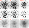 |
Fig. 1. Upper panel: original images of galaxy NGC 0628 before subtraction of diffuse background. Middle panel: images after subtraction of diffuse background, which show likely current star-forming regions. Lower panel: images of estimated diffuse background, showing its complex spatially varying nature. The images in a particular wavelength have the same flux scale limits. |
Adopting the same filtering scale length in the Nebulosity Filter as found for the SFR tracers, we also experimented with removing a diffuse background component from the H I map. To check the efficacy of Nebulosity Filter on HI maps, we reduced VLA B-configuration data for one of the typical galaxies (NGC 5055) in the sample, and created a moment 0 map with ∼6 arcsec resolution, which by construction should not contain much of the diffuse emission. Figure 2 shows that this image (right panel) is similar to the image obtained after processing the THINGS HI map of this galaxy with the Nebulosity Filter (middle panel). The fraction of diffuse background estimated in the two cases are in good agreement with each other, further showing the robustness of the Nebulosity Filter in separating diffuse background from the maps.
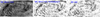 |
Fig. 2. Left panel: HI map of NGC 5055 obtained by combining data taken in B, C and D configurations of VLA. Middle panel: HI map of NGC 5055 obtained after processing the HI map in left panel with the Nebuliser, i.e. after subtraction of diffuse background. Right panel: HI map of NGC 5055 obtained by reducing data taken in B configuration of VLA, which should not contain any diffuse background. The images obtained via the two methods (middle panel and right panel) show similar structure, and similar fraction of diffuse background (∼76% from Nebuliser and ∼78% from B-configuration map). All images have the same flux scale limits. The pixel size of the HI (B-configuration) (right panel) is 0.5 arcsec while the other two have pixel size of 2 arcsec, same as CO map. |
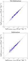 |
Fig. 3. Comparison of attenuation-corrected ΣSFR calculated from Hα and FUV before (upper panel) and after subtraction (lower panel) of diffuse background in SFR tracers for NGC 0628. The solid black line shows the best-fit to the data and the dashed red line is the one-to-one relation between the two recipes of ΣSFR. The scaling relation does not change significantly which shows that the subtraction of diffuse background is done consistently in all SFR tracers. |
The aperture-corrected fluxes (Sect. 3.1) from the original and subtracted images are used to calculate the fraction of diffuse background in the H II regions in Hα, FUV, MIPS 24 μm and H I. Since our aim is to remove the diffuse background in order to trace “current” star formation, the fraction of diffuse background in the selected regions is a more relevant quantity than the diffuse background in the entire galaxy. The combined results for each galaxy in the sample are tabulated in Table 3. On the entire images of the galaxies, we find a mean diffuse fraction of ∼34% in Hα, ∼43% in FUV, ∼37% in 24 μm, and ∼75% in atomic gas. The diffuse fraction in SFR tracers is in agreement with previous studies (∼30–50% diffuse ionised gas (DIG) related to Hα (Ferguson et al. 1996); 30–40% related to 24 μm in galactic centres and 20% in discs (Verley et al. 2009); at least a 40% diffuse UV (Liu et al. 2011)). The diffuse FUV fraction of 46% for NGC 5194 and 58% for NGC 3521 found in this work, are comparable to that (44% for NGC 5194 and 56% for NGC 3521) found by Liu et al. (2011). We find a fraction of 36% in 24 μm image of NGC 5194, which is close to the range (15–34%) given in Kennicutt et al. (2007). We find a Hα diffuse fraction of ∼17% in the central region of NGC 5194, which is mid-way between the values calculated by Blanc et al. (2009, 11%) and Liu et al. (2011, 32%). We note here that the diffuse fraction of Hα is more difficult to estimate accurately because of the necessity of scaling and subtracting the appropriate R-band continuum image from the Hα image. In all cases the fraction of diffuse background in the SFR tracers is significantly less than that in the atomic gas.
Percentage of diffuse background in each of the SFR tracers and atomic gas in the star-forming regions in the sample galaxies, along with the filtering scale used in Nebulosity Filter.
4. Results
4.1. Radial profiles
We study the spatial variation of diffuse background in SFR tracers in individual galaxies through their radial profiles, which are created by averaging over the pixels of the ΣSFR maps in elliptical annuli of constant width 12″ centred on the galaxies. ΣSFR maps are created by combining the optical/FUV and IR using formulae (4) and (5) and normalised by the de-projected area of each pixel. Figure 4 presents radial profiles of ΣSFR of the diffuse-background-subtracted data and ΣSFR of diffuse-background, showing the relative contribution of the two components (potential currently star-forming regions and diffuse background) in the star-forming galaxies. We find that the effect of the diffuse background in the faint outer star-forming regions is more significant than in the bright central star-forming region. For comparison, we created radial profiles for the original unsubtracted SFR and gas data presented in Appendix D. This comparison shows that ΣSFR even after subtraction of the diffuse background, follows a similar pattern to the molecular gas profile, highlighting the importance of molecular gas in star formation in the central regions of galaxies.
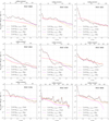 |
Fig. 4. Radial profiles of ΣSFR for all nine galaxies in sample after removal of diffuse background. The x-axis presents the galactocentric radius normalised by r25 (bottom) and in arcsecs (top). The y-axis presents ΣSFR in units of 10−3 M⊙ yr−1 kpc−2 (the scaling is performed for comparison with radial plots from original unsubtracted data in Fig. D.1). The brown and black curves denote ΣSFR(Hα + 24 μm) and ΣSFR(FUV + 24 μm) respectively obtained from the data where diffuse background is subtracted from the SFR tracers. The magenta and orange curves denote ΣSFR(Hα + 24 μm) and ΣSFR(FUV + 24 μm), respectively obtained from the diffuse background maps of the SFR tracers. |
4.2. Effect of subtraction of diffuse background in spatially-resolved Schmidt relations
We fitted ΣSFR versus Σgas in logarithmic space: log(ΣSFR) = Nlog(Σgas)+log A, using the orthogonal distance regression (ODR) algorithm (see reference for ODR in Virtanen et al. 2019), where maximum likelihood estimation of parameters is performed assuming that the distribution of errors on both axes is Gaussian. A S/N-cut of 3 was performed on all fits. In what follows we make use of unweighted fits for analysing the Schmidt relation variation. Using unweighted fits is standard practice in Schmidt relation studies (see for example Bigiel et al. 2008; Liu et al. 2011). Systematic uncertainties as large as 30–50% are present on both axes related to the SFR calibration and the CO-to-H2 conversion (Leroy et al. 2013), which explains the adoption of unweighted fits giving equal weight to each point on both axes. Problems with fitting power-laws in star-formation studies is a well-known issue (Blanc et al. 2009; Leroy et al. 2013; Casasola et al. 2015). In Appendix E, we revisit this problem by comparing different fits including unweighted fits and maximum likelihood fits weighted by uncertainties calculated as in Sect. 3.2. Including systematic calibrations errors of 20% on both axes is necessary to yield data models with reduced χ2 values of order unity. With this additional calibration error the difference between weighted fit and unweighted fit parameters lies within the measurement error.
To study the effect of inclusion and removal of diffuse background, we explored the spatially-resolved Schmidt relation on the original and diffuse-background-subtracted data for each individual galaxy. Figures 5 and 6 show this analysis for NGC 0628. The study on rest of the galaxies are shown in Appendix F. We have performed the entire analysis using both SFR(Hα + 24 μm) and SFR(FUV + 24 μm), though for space considerations we only show the Schmidt relations where SFR is determined using Hα. The use of Hα is justified by its ability to trace the current SFR due to its short age sensitivity (∼5 Myr), which is thus more relevant for the present analysis. However, the SFR estimated from Hα has been shown to deviate significantly from the true SFR accompanied by large scatter at lower fluxes/SFRs due to stochastic fluctuations. Given that the FUV is less sensitive to such effects, its use may be preferable as an SFR tracer (da Silva et al. 2014). To investigate this we analysed the sample using FUV as a SFR tracer and present the best-fit parameters for all Schmidt relations derived using Hα as well as FUV as SFR tracers. Tables 4 and 5 present the best-fit parameters (N, log A) for the original and subtracted data individually for each galaxy obtained from Hα and FUV, respectively. Table 6 compares the parameters of Schmidt relation obtained using Hα and FUV from the combined data of all galaxies. The uncertainty on N is ∼0.1 and log A is ∼0.1 dex for both Hα and FUV, and are obtained from the dispersion of values of these parameters from galaxy to galaxy. Thus, the parameters obtained from the two tracers agree with each other within the uncertainties, which adds confidence to our analysis.
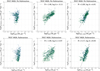 |
Fig. 5. Effect of subtraction of diffuse background in SFR tracers on spatially-resolved (∼560 pc) Schmidt relations in NGC 0628. Upper panel: analysis on the images with diffuse background (no subtraction). Lower panel: analysis on the images where diffuse background is subtracted. Left panel: ΣSFR versus ΣH I, middle panel: ΣSFR versus ΣH2. Right panel: ΣSFR versus ΣH I+H2. The error bars include the random error and systematic error on the flux measurements. The solid black line in each plot denotes the best-fit line to the data where equal weight is given to each data point on both axes. N and A denote the power-law index and the star-formation efficiency. The slope of the ΣSFR versus ΣH2 and ΣSFR versus ΣH I+H2 increases after subtraction of diffuse background. We note the saturation of H I at ∼10 M⊙ pc−2. Here, we assumed a Kroupa IMF and adopted a constant X(CO) factor = 2.0 × 1020 cm−2 (K km s−1)−1. |
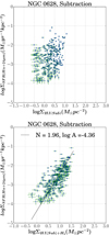 |
Fig. 6. Effect of subtraction of diffuse background in atomic gas and SFR tracers on spatially-resolved Schmidt relations in NGC 0628. Upper panel: ΣSFR versus ΣH I. Lower panel: ΣSFR versus ΣH I+H2. See caption of Fig. 5 for details on legends. |
Summary of best-fit parameters of Schmidt relation for individual galaxies.
Summary of Schmidt relation results for individual galaxies.
Comparison of parameters of Schmidt relation obtained by using different SFR tracers (Hα and FUV) by fitting data points from all galaxies.
We note here that the value of log A in Tables 4–6 has no practical meaning as it is representative of data points lying at the far lower-end of SFR and gas density. We have presented log A for the sake of comparison with global relation presented in Sect. 5.3. It would be more meaningful to compare log A in different galaxies at gas surface density of ∼10 M⊙ pc−2, where the majority of the data points lie.
4.2.1. Molecular gas and star-formation
We find that the scaling relation between ΣSFR and ΣH2 is approximately linear where no subtraction of diffuse background is done whereas the relation is super-linear when diffuse background is subtracted from the SFR tracers (middle panels in Figs. 5, F.1–F.8). Considering the individual galaxies, NGC 5457 is worth mentioning. For this galaxy, we find the slope of the molecular gas Schmidt relation before subtraction of the diffuse background to be very low at 0.66 (Fig. F.7, top-middle panel), which falls in the sub-linear regime (Shetty et al. 2013) and has been explained by bright diffuse CO emission (Shetty et al. 2014b,a). However, after subtraction of the diffuse background from the SFR tracers the Schmidt relation slope lies within the range found for the rest of the sample.
Taking the average of slopes found for each of the galaxies in the sample (Table 4), we find the slope to be 0.93 ± 0.06 before subtraction and 1.41 ± 0.094 after subtraction of diffuse background. We note that ΣSFR is estimated using Hα and 24 μm (Eq. (4)) in the above analysis. If we use instead the combination of FUV and 24 μm (Eq. (5)) to estimate ΣSFR, we find the slope to be 0.91 ± 0.07 before subtraction and 1.37 ± 0.11 after subtraction of diffuse background.
Figure 7 shows the spatially-resolved Schmidt relation between ΣSFR(Hα+24 μm) and ΣH2 for all galaxies in the sample on a single plot. The red line denotes the fit obtained above by averaging the slopes and intercepts from individual galaxies (Table 4) which gives equal weight to each galaxy. This method was adopted for a comparison with the pixel-by-pixel analysis of Bigiel et al. (2008). Each galaxy in principle should be weighted by the number of star-forming regions used in each galaxy. This can also be achieved by deriving parameters directly from the best-fit line to the spatially-resolved data of all galaxies (solid black line in Fig. 7). The best-fit slope is now 1.27 ± 0.1 (compared to average slope of 1.41 reported earlier) with a large rms scatter (0.34 dex). The formal fitting error in the slope is however small due to the large number of points (n ∼ 3000) used in the fit. We note here that owing to the large systematic uncertainties on the determination of quantities on each axes, the formal fitting error can not reflect the true error on the estimated best-fit parameters. Hence, we estimate the uncertainties from the dispersion in the best-fit parameters (N and log A) obtained for each galaxy.
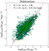 |
Fig. 7. Spatially-resolved molecular gas Schmidt relation (ΣSFR versus ΣH2) for all sample galaxies, where the diffuse background has been subtracted from the SFR tracers. The red line is the fit obtained by averaging N (power-law indices) and log A (star-formation efficiencies) from individual galaxies (Table 4). The solid black line shows the best-fit to the spatially-resolved data for all galaxies. A Kroupa IMF and a constant X(CO) factor = 2.0 × 1020 cm−2 (K km s−1)−1 have been assumed. |
4.2.2. H I saturation in all galaxies
We do not find any correlation between ΣSFR and ΣH I before or after subtraction of the diffuse background in the SFR tracers. Prior to subtraction of the diffuse H I background, saturation of H I is observed around ∼101.5 M⊙ pc−2 (leftmost panels in Figs. 5, F.1–F.8). After subtraction, the saturation of ΣH I is still observed but at a lower value of ∼10 M⊙ pc−2 (Figs. 6, upper panel and F.9).
4.2.3. Total gas and star-formation
The relation between ΣSFR and ΣH I+H2 is always super-linear irrespective of the background subtraction in SFR tracers (rightmost panels in Figs. 5, F.1–F.8). When diffuse background is removed from the SFR tracers , the slope steepens and varies from ∼1.65–3.18 depending on the relative quantity of ΣH I and ΣH2 (bottom-right panels in Figs. 5, F.1–F.8). In the majority of galaxies in the sample (e.g. NGC 3184 and NGC 6946), molecular gas surface density extends over two orders of magnitude whereas the atomic gas surface density saturates around 3–10 M⊙ pc−2. The dominance of molecular gas typically at the higher end of total gas surface density leads to a flatter slope in most galaxies compared to galaxies like NGC 0628 and NGC 3521 where neither gas component significantly dominates the higher end.
When diffuse background is removed from SFR tracers as well as atomic gas data, the slope of ΣSFR and ΣH I+H2 varies from ∼1.3–2.0 depending on the galaxy (Figs. 6, lower panel and F.10). The range of slope is significantly lower than the case with no background subtraction (∼1.19–2.54) or the case where the background is subtracted only from SFR tracers (∼1.65–3.18).
Figure 8 presents the spatially-resolved total gas Schmidt relation for all galaxies in the sample. Upper-left panel shows the original data where diffuse background is not subtracted, where we observe a bimodal relation. Upper-right panel shows the Schmidt relation where diffuse background is subtracted from SFR tracers only, and the slope is super-linear. Lower-left panel shows data where diffuse background is subtracted from SFR tracers as well as atomic gas data. Here, the best-fit line (solid black) to the spatially-resolved data (blue dots with green error bars) for all galaxies results in a slope of ∼1.47 ± 0.08 with a scatter of 0.27. The reported error on the slope is the dispersion in slopes obtained for each galaxy in the sample. Thus, comparing the upper-left panel with other panels in Fig. 8, we find that the removal of the diffuse background from the SFR tracers results in a continuous relation. In Fig. G.1, we present the equivalent figures of Fig. 8, where SFR is obtained using FUV instead of Hα. As mentioned beforehand, change of SFR tracer do not result in any significant changes in the best-fit parameters or in general trend of spatially-resolved total gas Schmidt relation (see Table 6 for a comparison).
 |
Fig. 8. Spatially-resolved total gas Schmidt relation (ΣSFR and ΣH I+H2). In each panel, blue dots with green error bars are the spatially-resolved data, and the solid black line shows the best-fit to the spatially-resolved data for all galaxies. We have assumed a Kroupa IMF and adopted a constant X(CO) factor = 2.0 × 1020 cm−2 (K km s−1)−1. Upper-left panel: no subtraction of diffuse background is done. The vertical dotted line corresponds to 10 M⊙ pc−2 around which atomic gas surface density saturates. Upper-right panel: the diffuse background is subtracted from the SFR tracers. The solid yellow line and the dashed red line denote star-formation relation from Elmegreen 2015 (E2015) and correspond to velocity dispersion (σ) of 6 km s−1 and 11 km s−1 respectively. Lower-left panel: the diffuse background is subtracted from the SFR tracers as well as from H I. Lower-right panel: the diffuse background is subtracted from the SFR tracers, HI and CO. The solid yellow solid line on lower panels corresponds to the star-formation relation based on a dynamical model from Elmegreen (2015) obtained at a constant scale height of H = 100 pc. See text in Sect. 5.1 for further details on models. |
5. Discussion
5.1. Comparison with models
In Fig. 8, we compare spatially-resolved total gas Schmidt relations with dynamical models of star formation where we take into account disc flaring as discussed in Elmegreen (2015). The flaring of the gas disc is parametrised by the scale height H of the gas, which varies with surface gas density such that H ∝ σ2/Σgas. where σ is the gas velocity dispersion. For a uniform spherical gas cloud of density ρ ∝ Σgas/H, star formation is related to the available gas reservoir by ΣSFR = ϵffΣgas/tff where the free-fall time for cloud collapse  and ϵff denotes the efficiency per unit free-fall time. For σ = 6 km s−1 (Kennicutt 1989) and ϵff = 0.01 (Krumholz & Tan 2007), star formation is then expected to follow:
 (6)
(6)
as derived by Elmegreen (2015). We overlay this relation (6) as the solid yellow line on Fig. 8 (upper-right panel), which shows the total gas spatially-resolved Schmidt relation where the diffuse background has been subtracted from the SFR tracers only. The dashed red line corresponds to a star-formation relation where we assume σ = 11 km s−1 based on more recent THINGS galaxies (Leroy et al. 2009 and also see Tamburro et al. 2009). We find that the model with both values of σ is in reasonable agreement with our data.
For the total gas Schmidt relation where the diffuse background is subtracted from SFR tracers as well as atomic gas, we use the dynamical model with a constant scale height, meaning that, there is no flaring. In this case for a fixed scale height of H = 100 pc and ϵff = 0.01, Elmegreen (2015) derived the following star-formation relation:
 (7)
(7)
The above Eq. (7) corresponds to the yellow line in Fig. 8 (lower-left panel) showing a very good agreement with the best-fit line to the spatially-resolved data. The agreement of the model with the background subtracted atomic data probably indicates that removing the diffuse background component using the Nebulosity Filter mainly removes the atomic gas from the vertically-extended regions in the flared outskirts of galaxies, effectively rendering the scale height to be constant throughout the sample of galaxies. While it is expected that the star-forming atomic gas is most likely the cold neutral medium component of the ISM, it is however difficult to infer the nature of this component with the current data.
We also tested the potential impact of diffuse CO emission by applying the Nebulosity Filter on CO maps adopting the same parameters used for removing diffuse background in the SFR tracers. We then revisited the total gas Schmidt relation using the background subtracted SFR, atomic and molecular gas data and compared with predictions from the dynamical models discussed earlier (Figs. 8 and G.1, lower-right panels). It is perhaps not surprising that models incorporating flaring do not agree with these Schmidt relation parameters because the scale height of the molecular gas disc is significantly less than the neutral gas and also varies less with radius as found for the edge-on galaxy NGC 891 (Yim et al. 2011 and also see Barnes et al. 2012; Bacchini et al. 2019a). Hence, we do not expect any significant large scale diffuse CO emission that could be reliably picked up by our current analysis method.
We note that we found a non-linear molecular gas Schmidt relation (Fig. 7), where the diffuse background is subtracted only from SFR tracers. This result is also in agreement with Elmegreen (2015), who mentions that the molecular gas relation should not be exactly linear because of the change of ϵff for different molecules considering the effects of molecule depletion on grains or change in gas sub-structure due to turbulence.
In summary, a comparison with dynamical models incorporating flaring effects indicates that a diffuse component is present in SFR tracers as well as atomic gas, which does not contribute to current star formation. Though this model was originally meant to explain the origin of a power-law index of 1.5 for the inner regions of spiral galaxies and power-law index of 2 for the outskirts and for dwarf irregular galaxies, we find that accounting for vertically-extended diffuse background in atomic gas leads to a single power-law index of 1.5 for the inner as well as outer regions of spiral galaxies. Further works need to be done to test if accounting for diffuse background could lead to a power-law index of 1.5 in dwarf galaxies as well.
5.2. Comparison with literature
The current work is a spatially-resolved star-formation study where diffuse background has been taken into account in both the SFR tracers as well as the atomic gas while studying the Schmidt relations. Earlier spatially-resolved star-formation studies have either been through radial-profile analysis (Wong & Blitz 2002) or through point-by-point analysis (e.g. Bigiel et al. 2008; Kennicutt et al. 2007; Liu et al. 2011), where either diffuse background is not considered at all (e.g. Bigiel et al. 2008; Wong & Blitz 2002) or it is accounted for in the SFR tracers (e.g. Kennicutt et al. 2007; Liu et al. 2011; Momose et al. 2013; Morokuma-Matsui & Muraoka 2017) or in the molecular gas (Rahman et al. 2011) but not in the atomic gas.
The saturation of H I is a common result found in all works. From the aperture photometry analysis, we find the mean saturation value to be 16 ± 8 M⊙ pc−2 when diffuse background is not subtracted, which is consistent with the value of ∼25 M⊙ pc−2 derived by aperture photometry analysis of Kennicutt et al. (2007) on NGC 5194. Our radial profile analysis (Fig. D.1) also shows a saturation below 10 M⊙ pc−2 in agreement with ∼9–10 M⊙ pc−2 derived by earlier radial profile analyses (Wong & Blitz 2002; Bigiel et al. 2008). The difference in results can be attributed to the different approaches adopted in these studies. Unlike aperture photometry, pixel-by-pixel analysis or radial profile analysis does not take into account the flux lost in the adjacent pixels, which might be the cause of the lower level of saturation for H I in these analyses. Roychowdhury et al. (2015) finds a power-law slope of 1.5 between ΣSFR and ΣH I, which appears to be in contrast with this and previous studies mentioned above and may be simply because Roychowdhury et al. (2015) exclude regions detected in CO to concentrate mainly on regions dominated by HI, while other studies (including this one) do not make such selections. We discuss the agreement of results of Roychowdhury et al. (2015) and the current work later in Sect. 5.3.
Comparison of the power-law index of the molecular gas Schmidt relation found by pixel-by-pixel analysis (Bigiel et al. 2008) and aperture photometry (upper panels in Figs. 5, F.1–F.8) for individual galaxies in the sample shows a large variation in the case where diffuse background is not subtracted. However, results from the two works agree with each other statistically as found in Sect. 4.2.1. The slope of the molecular gas Schmidt relation reported by Bigiel et al. (2008) (0.96 ± 0.07) agrees within error with the slope we found here by averaging the slopes found for individual galaxies (i.e. 0.93±0.06 using Hα and 0.91 ± 0.07 derived using FUV). Hence, both of these works show that before background subtraction, ΣSFR scales linearly with molecular gas surface density statistically, in agreement with various other studies (e.g. Liu et al. 2011; Schruba et al. 2011; Leroy et al. 2013). The total gas Schmidt relation before subtraction of diffuse background shows a knee at 10 M⊙ pc−2, which is in agreement with the results of Bigiel et al. (2008). Compared to the bimodal relation of Bigiel et al. (2008), we find a higher dispersion at the lower end of the total gas Schmidt relation. This is simply because Bigiel et al. (2008) only include the molecular gas data in the regime where ΣH2 > 3 M⊙ pc−2 for HERACLES data and ΣH2 > 10 M⊙ pc−2 for BIMA SONG data. Since H I saturates around this cut-off value for all the galaxies, the total gas Schmidt relation at the lower end is basically the atomic gas Schmidt relation. In our work, by using forced aperture photometry based on positions derived from the Hα map, we can legitimately include regions with minimal ab-initio detection of molecular gas, particularly in the outer regions of galaxies. Our results are supported by those of Schruba et al. (2011), whose stacking analysis allow them to trace the molecular gas surface density even in the outskirts of the galaxy. They report marginal CO detections which are as low as 0.1 M⊙ pc−2 equivalent to our S/N > 3 cut. Hence our analysis shows that the Schmidt relations on sub-galactic scales do not depend on the method adopted – aperture photometry or pixel-by-pixel analysis.
Some studies (Heyer et al. 2004; Komugi et al. 2005; Momose et al. 2013) have found a super-linear molecular Schmidt relation even using data where diffuse background was not subtracted from the SFR tracers. However, all of these studies have used CO(1–0) data to trace the molecular gas, instead of CO(2–1) used in this work. The excitation for CO(2–1) is significantly affected by a slight change in the kinetic temperature and volume density of molecular gas, which in turn affects the power-law index of the Schmidt relation (Momose et al. 2013). The change of the power-law index resulting from using a different molecular gas tracer (for example, CO(1–0), CO(3–2), HCN(1–0)) has been observed before by other studies as well (Narayanan et al. 2008; Bayet et al. 2009; Iono et al. 2009).
Subtraction of the diffuse background in SFR tracers naturally leads to an increase in the slope of the molecular gas Schmidt relation in all galaxies in the sample. This result is in agreement with Liu et al. (2011), who reports that the subtraction of diffuse background in SFR tracers leads to a super-linear slope of the molecular gas Schmidt relation from their analysis on two galaxies (NGC 5194 and NGC 3521). Adopting the same method of subtraction as Liu et al. (2011), Momose et al. (2013), and Morokuma-Matsui & Muraoka (2017) found the steepening of slope in agreement with our study. Rahman et al. (2011) also shows that the spatially-resolved molecular Schmidt relation can be non-linear if SFR tracers contain a significant fraction of diffuse emission. Leroy et al. (2013) subtracted diffuse background only in the 24 μm data before combining it to Hα and found subtle effects in the molecular gas Schmidt relation. This is likely due to the presence of diffuse background in Hα as well, which should also be taken into account while studying the current star-formation rate. However, their results are consistent with ours in the sense of increase in scatter of the relation after removal of diffuse background. After subtraction of the diffuse background in SFR tracers, the best-fit line to our spatially-resolved data gives a slope of 1.26 ± 0.10 for the molecular gas Schmidt relation. This result is in agreement with previous works (Kennicutt et al. 2007; Liu et al. 2011). Using integral field spectroscopic data (IFS) for NGC 5194, Blanc et al. (2009) determined the diffuse emission in Hα using the [S II]/Hα line ratio and found the slope of the molecular gas Schmidt relation to be 0.84 in this galaxy. However, a direct comparison between their work and ours is complicated by the large differences in the methodology adopted, particularly the difference in data (photometric versus IFS), physical scale of study (0.5–2 kpc versus ∼170 pc) and diffuse background estimation.
For both molecular and total gas Schmidt relations of individual galaxies, we find that the rms scatter increases after subtraction of diffuse background (Figs. 5, F.1–F.8). This result is consistent with previous works (Liu et al. 2011; Leroy et al. 2013; Morokuma-Matsui & Muraoka 2017), which have employed different techniques for diffuse background subtraction. This consistency in the increase in scatter in the Schmidt relation in a log-log domain may point towards an astrophysical origin but is quite likely a result of removal of diffuse signal whilst minimally changing the underlying noise.
5.3. Comparison with the global Kennicutt–Schmidt relation
Figure 9 presents a summary of the Schmidt relation with all the star-forming regions from our galaxy sample together with the integrated measurements of starburst and spiral galaxies taken from Kennicutt (1998b), low surface brightness galaxies (LSBs, orange triangles) from Wyder et al. (2009), dwarf irregulars (dIrrs, pink squares) from Roychowdhury et al. (2017), which is a sub-sample of Roychowdhury et al. (2014). For the spatially-resolved data, the diffuse background has been subtracted from the SFR tracers and the atomic gas, and we adjusted the IMF and X(CO) factor of our spatially-resolved data to those of integrated data (i.e. a Salpeter IMF and an X(CO) factor of 2.8 × 1020 cm−2 (K km s−1)−1). Hence, we find the following best-fit line:
 (8)
(8)
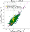 |
Fig. 9. Comparison of the spatially-resolved total gas Schmidt relation for nine spiral galaxies in this work with the global Kennicutt–Schmidt relation of the starbursts (black stars) and spirals (yellow dots) taken from Kennicutt (1998b), low surface brightness galaxies (LSBs, orange triangles) from Wyder et al. (2009) and dwarf irregular galaxies (dIrrs, pink squares) from Roychowdhury et al. (2017). The diffuse background has been subtracted from the SFR tracers as well as from the atomic gas for the spatially-resolved data (blue dots with green error bars). These local measurements assume a Salpeter IMF and an X(CO) factor of 2.8 × 1020 cm−2 (K km s−1)−1 to match the parameters adopted in Kennicutt (1998b). The pink line represents the global Kennicutt–Schmidt relation from Kennicutt (1998b) while the solid black line is the best-fit line to the spatially-resolved data from all galaxies in this work. |
Interestingly, the above best-fit line passes through integrated data corresponding to dIrrs (Roychowdhury et al. 2017) and LSBs (Wyder et al. 2009), which only has atomic gas observations, and is in agreement with the conclusions of Roychowdhury et al. (2015), who suggest a power law slope of ∼1.5 in the HI-dominated regions.
The slope of the global and local best-fit lines is identical within the errors which we reason as follows. The radial profiles of SFR (Fig. 4) highlight that the diffuse background affects the low surface brightness outer regions of galaxies more significantly than the central regions of galaxies. Since the global Kennicutt–Schmidt relation targets entire star-forming discs of galaxies, or bright star-forming regions, the effect of any diffuse background either averages out or is negligible. However, at local scales, the effect on the Schmidt relation becomes prominent when star-forming peaks as well as regions dominated by diffuse background are selected. That is possibly a reason why the global Kennicutt–Schmidt relation and local Schmidt relation have similar slopes. We note here that the similarity of slope in local and global results must be interpreted with caution, given that there has been much debate about the relative importance of molecular and atomic gas in the formation of stars, and the presence of diffuse H I component is even more uncertain.
Furthermore, there is an offset in the zeropoints, that is, −3.9 in this study versus −3.6 in the global relation. A Kolmogorov–Smirnov test on the global and spatially-resolved data shows that the observed offset in the zeropoints of the global and local results is significant enough to affect the overall interpretation of the star-formation relation. There are several possible reasons for this difference in zero-points. In local sample selection, the chosen sub-regions of star formation in any spatially-resolved study will be biased by the selection criteria. For example, in this study we used Hα luminous regions but given our understanding of the formation of stars from molecular gas clouds, we could also have selected star-forming regions on the basis of molecular gas peaks. There is no such sampling effect in global studies. In addition, Kennicutt et al. (2007) describes the filling factor of star-forming regions in the disc of galaxies as a potential cause of the observed offset. Other reasons which can contribute to the observed offset are the different SFR calibration recipes at local and global scale. We note here that the non-negligible uncertainties due to age and the IMF are present in the conversion factor of luminosity to SFR. While comparing the spatially-resolved Schmidt relation with the global Kennicutt-Schmidt Law, we took into account the IMF which contributes significantly to the differences in SFR calibration at global and local scale (in Sect. 3.3) but we did not take into account for example, the age of the H II regions. Hence, it is not surprising to see differences in the global versus local total gas Schmidt relations.
Though the slope of the combined total gas spatially-resolved Schmidt relation matches the global Schmidt–Kennicutt relation, there is considerable variation in slopes from galaxy to galaxy. Such variation has been observed before in previous studies, even without the subtraction of diffuse background (see e.g. Wong & Blitz 2002; Boissier et al. 2003; Bigiel et al. 2008) though note here the subtraction of diffuse background from H I gas has led to a decrease in the variation of slopes. To explore the variation in the background subtracted data, we examined the variation of slope with respect to the ratio of the molecular-to-atomic gas surface density (within the analysis apertures) for all galaxies, however we did not find any trend. The large variation in slopes from galaxy to galaxy may also result from the higher uncertainties at lower SFRs (da Silva et al. 2014).
The variation of X(CO) factor within galaxies may be another cause of the observed variation of slopes, for example, by using a radially-varying metallicity-dependent X(CO) factor, Boissier et al. (2003) derived a steeper slope (∼2). Sandstrom et al. (2013) reports a radial variation of X(CO) in eight out of nine galaxies in our sample, with an overall decrease of 0.3 dex in the centre of galaxies. Since in our work, we have assumed a constant X(CO) factor (for comparison with other works), it is likely that the reported molecular gas surface densities are overestimated in the centres. It is possible that the variation of slope from galaxy-to-galaxy will further reduce if we adopt a radially-varying X(CO) factor in conjunction with diffuse background subtraction in SFR tracers and atomic gas. In our analysis, we did not take into account a local diffuse CO emission, mainly because of the poor resolution of CO map. However, various studies suggest the presence of a diffuse molecular gas forming at least 30% of the total CO intensity (see Shetty et al. 2014b, and references therein). As in the case of SFR tracers and atomic gas, a diffuse CO component will affect the lower intensity regions more than the higher intensity regions. This will result in the flattening of the slope both for the molecular gas and total gas Schmidt relations. Like SFR tracers and atomic gas, the fraction of CO bright diffuse gas will also vary from galaxy to galaxy. Correcting for the diffuse CO gas may result in a reduced overall variation of slopes.
Another possible source of systematics affecting the derived slopes are selection effects and sample biases from using the Hα maps for picking out the star-forming regions. Ideally, to check this we should use the peaks of molecular gas (from CO maps), as indicators of star-forming regions. However, to check the effect of such systematics, we would need high resolution molecular gas maps, where the peaks can be readily resolved. Kruijssen & Longmore (2014) discusses how centring an aperture on gas or star-forming peaks might introduce a spatial-scale-dependent bias of the gas depletion time-scale and allows us to quantify this bias via an uncertainty principle for star formation. However, we could not use this principle to quantify the potential bias because it is only applicable to the case where the depletion time-scale is constant. In our study, the subtraction of diffuse background in SFR tracers has resulted in super-linear molecular gas Schmidt relation. The total gas Schmidt relation is super-linear irrespective of background subtraction in SFR tracers or atomic gas. The super-linearity implies that the depletion time-scale is not constant. Further theoretical and observation work needs to be done for quantification of such biases.
6. Conclusion
In summary, we have studied the spatially-resolved molecular and total gas Schmidt relation individually for nine galaxies, and also the overall combined fit for all galaxies for both molecular and total gas (Figs. 7 and 8), by performing aperture photometry on the regions selected from Hα maps. Though we find the slopes of the global and local total gas Schmidt relation to be similar, it is difficult to draw conclusions from this similarity especially when a large variation in slopes has been observed from galaxy to galaxy. The smaller scatter in log-log space in the total gas Schmidt relation compared to the molecular gas Schmidt relation may simply be the result of having more signal with respect to the noise contributions from the combination of H I and H2. However, it may also indicate that atomic gas may be contributing to the star formation. In the spatially-resolved total gas Schmidt relation, we obtain a slope of 1.4 when diffuse background is subtracted from SFR tracers and the atomic gas. We find that the fraction of diffuse atomic gas in all galaxies is higher than the fraction of diffuse background in the SFR tracers (Table 3) at the same spatial scale. It constitutes ∼37–80% depending on the galaxy. Excluding NGC 5457, diffuse atomic gas is > 50% in all galaxies. This might indicate that at the local scale in projection, a vast amount of atomic gas (i.e. diffuse background) in the ISM is not relevant for star formation. However, about 20–50% of this atomic gas is available locally for star formation and hence its role can not be neglected. It is probably the cold component of the atomic gas, that is, the cold neutral medium rather than the warm neutral medium, which contributes to star formation, though it is difficult to infer the nature of the diffuse background seen in atomic gas on the basis of the current data.
A comparison with the dynamical model of Elmegreen 2015 indicates that the diffuse background in HI gas is likely the vertically-extended atomic gas which does not contribute to star formation. It is probably both atomic and molecular gas in the disc (rather than out of disc) of galaxies which contribute to star formation. Diffuse CO emission is not compatible with the dynamical model considered here, indicating that molecular gas is still the prime driver of star formation. However, the role of atomic gas in star formation especially in the outskirts of galaxies should not be neglected, where there is an abundance of atomic gas with no detection of molecular gas. Moreover, in the nearby Universe, atomic gas forms a large fraction of cold gas reservoir in galaxies. The molecular gas which directly feeds star formation, constitutes only ∼30% of the cold gas (Catinella et al. 2010; Saintonge et al. 2011; Boselli et al. 2014). A recent study by Cortese et al. (2017) also shows that the gas reservoirs of star-forming discs at z ∼ 0.2 are not predominantly molecular. So in such systems, atomic gas seems to be the source of star formation. Though from the current study it is difficult to infer the relative importance of atomic and molecular gas in star formation, we may say that both of the components (atomic and molecular) of the ISM may be collectively important for forming stars.
In this study, we find that the dynamical models of star formation with a constant scale height throughout galaxy discs explains very well the spatially-resolved total gas Schmidt relation when diffuse background from SFR tracers as well as H I are removed. The consideration of this diffuse background results in a single power-law relation between ΣSFR and ΣH I + H2 with power-law index of 1.5 in both inner and outer parts of spiral galaxies. Furthermore, a super-linear Schmidt relation at local and global scales would imply the dominant role of non-linear processes in driving star formation at spatially-resolved as well as global scales, and a non-constant star formation efficiency, or time scale, for different gas surface densities at different spatial scales.
To explore the above hypotheses, we need to study the distribution of different phases of the ISM at the scales of H II regions, their spatial correlation, and also study these star-forming regions in different evolutionary stages. This will allow us to understand the relative importance of the different components of the ISM responsible for star formation and the nature of diffuse emission in SFR tracers, for example warm ionised medium (DIG) traced by Hα. It is now possible to study in great detail the characteristic properties of DIG in the nearby star-forming regions, with the advent of IFS facilities like the Multi-Unit Spectroscopic Explorer (MUSE) and the Keck Cosmic Web Imager (KCWI). Moreover, the IFS technique allows us to correct the internal dust-attenuation in the galaxies directly from the Balmer-decrement (Hα:Hβ:Hγ), bypassing the use of the infrared (24 μm) images, which means that we can reduce the uncertainties related to the diffuse component in infrared images. Similarly, observational facilities like the Atacama Large Millimeter/submillimeter Array (ALMA), the Submillimeter Array (SMA), the Robert C. Byrd Green Bank Telescope (GBT) are apt to characterise the neutral gas (both atomic and molecular) in the nearby star-forming regions. Thus these combined analyses will help us better understand the intricacies of star formation.
IRAF is distributed by the National Optical Astronomy Observatory, which is operated by the Association of Universities for Research in Astronomy (AURA) under a cooperative agreement with the National Science Foundation.
error = standard deviation/ where N is the total number of galaxies.
Infrared maps of galaxies are brighter in the inner regions of galaxies compared to the outer regions.
Acknowledgments
We sincerely thank the reviewer of the paper whose helpful comments and suggestions greatly improved the paper. It is a pleasure to thank Rob Kennicutt for providing us with archival KINGFISH data, reading manuscripts of this paper and giving invaluable comments which greatly improved the scientific presentation of this analysis. N. K. also thanks Gareth Jones for helping with CASA. N. K. acknowledges the support from Institute of Astronomy, Cambridge and the Nehru Trust for Cambridge University during PhD, and the Schlumberger Foundation during the post-doc. This research made use of the NASA/IPAC Extragalactic Database (NED) which is operated by the Jet Propulsion Laboratory, California Institute of Technology, under contract with the National Aeronautics and Space Administration; SAOImage DS9, developed by Smithsonian Astrophysical Observatorys; Astropy, a community-developed core Python package for Astronomy.
Note added in proof. After this paper was accepted, we became aware of another recent paper which supports the results of our work: Wilson et al. (2019) find a super-linear-resolved Schmidt relation for five U/LIRGs (their Fig. 1) consistent with our results (Fig. 9). This also supports the general interpretation of this work by way of a comparison with the dynamical models of Elmegreen (2015) at a constant scale height.
References
- Azeez, J. H., Hwang, C.-Y., Abidin, Z. Z., & Ibrahim, Z. A. 2016, Sci. Rep., 6, 26896 [NASA ADS] [CrossRef] [Google Scholar]
- Bacchini, C., Fraternali, F., Iorio, G., & Pezzulli, G. 2019a, A&A, 622, A64 [NASA ADS] [CrossRef] [EDP Sciences] [Google Scholar]
- Bacchini, C., Fraternali, F., Pezzulli, G., et al. 2019b, A&A, 632, A127 [NASA ADS] [CrossRef] [EDP Sciences] [Google Scholar]
- Barnes, K. L., van Zee, L., Côté, S., & Schade, D. 2012, ApJ, 757, 64 [NASA ADS] [CrossRef] [Google Scholar]
- Bayet, E., Gerin, M., Phillips, T. G., & Contursi, A. 2009, MNRAS, 399, 264 [NASA ADS] [CrossRef] [Google Scholar]
- Bigiel, F., Leroy, A., Walter, F., et al. 2008, AJ, 136, 2846 [NASA ADS] [CrossRef] [Google Scholar]
- Bigiel, F., Leroy, A., Walter, F., et al. 2010, AJ, 140, 1194 [NASA ADS] [CrossRef] [Google Scholar]
- Blanc, G. A., Heiderman, A., Gebhardt, K., Evans, II., N. J., & Adams, J. 2009, ApJ, 704, 842 [NASA ADS] [CrossRef] [Google Scholar]
- Boissier, S., Prantzos, N., Boselli, A., & Gavazzi, G. 2003, MNRAS, 346, 1215 [NASA ADS] [CrossRef] [Google Scholar]
- Boquien, M., Buat, V., & Perret, V. 2014, A&A, 571, A72 [NASA ADS] [CrossRef] [EDP Sciences] [Google Scholar]
- Boquien, M., Kennicutt, R., Calzetti, D., et al. 2016, A&A, 591, A6 [NASA ADS] [CrossRef] [EDP Sciences] [Google Scholar]
- Boselli, A., Cortese, L., Boquien, M., et al. 2014, A&A, 564, A66 [NASA ADS] [CrossRef] [EDP Sciences] [Google Scholar]
- Bromm, V., & Larson, R. B. 2004, ARA&A, 42, 79 [NASA ADS] [CrossRef] [EDP Sciences] [Google Scholar]
- Calzetti, D., Kennicutt, Jr., R. C., Bianchi, L., et al. 2005, ApJ, 633, 871 [NASA ADS] [CrossRef] [Google Scholar]
- Calzetti, D., Kennicutt, R. C., Engelbracht, C. W., et al. 2007, ApJ, 666, 870 [NASA ADS] [CrossRef] [Google Scholar]
- Casasola, V., Hunt, L., Combes, F., & García-Burillo, S. 2015, A&A, 577, A135 [NASA ADS] [CrossRef] [EDP Sciences] [Google Scholar]
- Catinella, B., Schiminovich, D., Kauffmann, G., et al. 2010, MNRAS, 403, 683 [NASA ADS] [CrossRef] [Google Scholar]
- Chandar, R., Leitherer, C., Tremonti, C. A., et al. 2005, ApJ, 628, 210 [NASA ADS] [CrossRef] [Google Scholar]
- Cortese, L., Catinella, B., & Janowiecki, S. 2017, ApJ, 848, L7 [NASA ADS] [CrossRef] [Google Scholar]
- Crocker, A. F., Calzetti, D., Thilker, D. A., et al. 2013, ApJ, 762, 79 [NASA ADS] [CrossRef] [Google Scholar]
- Dame, T. M., Hartmann, D., & Thaddeus, P. 2001, ApJ, 547, 792 [NASA ADS] [CrossRef] [Google Scholar]
- da Silva, R. L., Fumagalli, M., & Krumholz, M. R. 2014, MNRAS, 444, 3275 [NASA ADS] [CrossRef] [Google Scholar]
- Draine, B. T. 2011, Physics of the Interstellar and Intergalactic Medium (Princeton: Princeton University Press) [Google Scholar]
- Draine, B. T., & Li, A. 2007, ApJ, 657, 810 [NASA ADS] [CrossRef] [Google Scholar]
- Elmegreen, B. G. 2015, ApJ, 814, L30 [NASA ADS] [CrossRef] [Google Scholar]
- Elmegreen, B. G., & Elmegreen, D. M. 1987, ApJ, 320, 182 [NASA ADS] [CrossRef] [Google Scholar]
- Evans, II., N. J. 1999, ARA&A, 37, 311 [NASA ADS] [CrossRef] [Google Scholar]
- Ferguson, A. M. N., Wyse, R. F. G., Gallagher, III., J. S., & Hunter, D. A. 1996, AJ, 111, 2265 [NASA ADS] [CrossRef] [Google Scholar]
- Fukui, Y., Kawamura, A., Wong, T., et al. 2009, ApJ, 705, 144 [NASA ADS] [CrossRef] [Google Scholar]
- Gil de Paz, A., Boissier, S., Madore, B. F., et al. 2007, ApJS, 173, 185 [NASA ADS] [CrossRef] [Google Scholar]
- Glover, S. 2005, Space Sci. Rev., 117, 445 [NASA ADS] [CrossRef] [Google Scholar]
- Glover, S. C. O., & Clark, P. C. 2012, MNRAS, 421, 9 [NASA ADS] [Google Scholar]
- Goldsmith, P. F., & Li, D. 2005, ApJ, 622, 938 [NASA ADS] [CrossRef] [Google Scholar]
- Goodman, A. A., Rosolowsky, E. W., Borkin, M. A., et al. 2009, Nature, 457, 63 [NASA ADS] [CrossRef] [PubMed] [Google Scholar]
- Gordon, K. D., Clayton, G. C., Witt, A. N., & Misselt, K. A. 2000, ApJ, 533, 236 [NASA ADS] [CrossRef] [Google Scholar]
- Gordon, K. D., Rieke, G. H., Engelbracht, C. W., et al. 2005, PASP, 117, 503 [NASA ADS] [CrossRef] [Google Scholar]
- Hayashi, K., Okamoto, R., Yamamoto, H., et al. 2019, ApJ, 878, 131 [NASA ADS] [CrossRef] [Google Scholar]
- Heyer, M. H., Corbelli, E., Schneider, S. E., & Young, J. S. 2004, ApJ, 602, 723 [NASA ADS] [CrossRef] [Google Scholar]
- Iono, D., Wilson, C. D., Yun, M. S., et al. 2009, ApJ, 695, 1537 [NASA ADS] [CrossRef] [Google Scholar]
- Johnson, B. D., Weisz, D. R., Dalcanton, J. J., et al. 2013, ApJ, 772, 8 [NASA ADS] [CrossRef] [Google Scholar]
- Kennicutt, Jr., R. C. 1989, ApJ, 344, 685 [NASA ADS] [CrossRef] [Google Scholar]
- Kennicutt, Jr., R. C. 1998a, ARA&A, 36, 189 [Google Scholar]
- Kennicutt, Jr., R. C. 1998b, ApJ, 498, 541 [NASA ADS] [CrossRef] [Google Scholar]
- Kennicutt, R. C., & Evans, N. J. 2012, ARA&A, 50, 531 [NASA ADS] [CrossRef] [Google Scholar]
- Kennicutt, Jr., R. C., Armus, L., Bendo, G., et al. 2003, PASP, 115, 928 [NASA ADS] [CrossRef] [Google Scholar]
- Kennicutt, Jr., R. C., Calzetti, D., Walter, F., et al. 2007, ApJ, 671, 333 [NASA ADS] [CrossRef] [Google Scholar]
- Kennicutt, Jr., R. C., Hao, C.-N., Calzetti, D., et al. 2009, ApJ, 703, 1672 [NASA ADS] [CrossRef] [Google Scholar]
- Kennicutt, R. C., Calzetti, D., Aniano, G., et al. 2011, PASP, 123, 1347 [NASA ADS] [CrossRef] [Google Scholar]
- Komugi, S., Sofue, Y., Nakanishi, H., Onodera, S., & Egusa, F. 2005, PASJ, 57, 733 [NASA ADS] [Google Scholar]
- Kritsuk, A. G., Ustyugov, S. D., & Norman, M. L. 2011, in Computational Star Formation, eds. J. Alves, B. G. Elmegreen, J. M. Girart, & V. Trimble, IAU Symp., 270, 179 [NASA ADS] [Google Scholar]
- Kroupa, P. 2001, in Dynamics of Star Clusters and the Milky Way, eds. S. Deiters, B. Fuchs, A. Just, R. Spurzem, & R. Wielen, ASP Conf. Ser., 228, 187 [NASA ADS] [Google Scholar]
- Kruijssen, J. M. D., & Longmore, S. N. 2014, MNRAS, 439, 3239 [NASA ADS] [CrossRef] [Google Scholar]
- Krumholz, M. R. 2012, ApJ, 759, 9 [NASA ADS] [CrossRef] [Google Scholar]
- Krumholz, M. R. 2014, Phys. Rep., 539, 49 [NASA ADS] [CrossRef] [Google Scholar]
- Krumholz, M. R., & Tan, J. C. 2007, ApJ, 654, 304 [NASA ADS] [CrossRef] [Google Scholar]
- Leitherer, C., Schaerer, D., Goldader, J. D., et al. 1999, ApJS, 123, 3 [NASA ADS] [CrossRef] [Google Scholar]
- Leroy, A. K., Walter, F., Brinks, E., et al. 2008, AJ, 136, 2782 [NASA ADS] [CrossRef] [Google Scholar]
- Leroy, A. K., Walter, F., Bigiel, F., et al. 2009, AJ, 137, 4670 [NASA ADS] [CrossRef] [Google Scholar]
- Leroy, A. K., Bigiel, F., de Blok, W. J. G., et al. 2012, AJ, 144, 3 [NASA ADS] [CrossRef] [Google Scholar]
- Leroy, A. K., Walter, F., Sandstrom, K., et al. 2013, AJ, 146, 19 [NASA ADS] [CrossRef] [Google Scholar]
- Li, H.-B., Goodman, A., Sridharan, T. K., et al. 2014, Protostars and Planets VI, 101 [Google Scholar]
- Liu, G., Koda, J., Calzetti, D., Fukuhara, M., & Momose, R. 2011, ApJ, 735, 63 [NASA ADS] [CrossRef] [Google Scholar]
- Lonsdale Persson, C. J., & Helou, G. 1987, ApJ, 314, 513 [NASA ADS] [CrossRef] [Google Scholar]
- Mac Low, M.-M., & Klessen, R. S. 2004, Rev. Mod. Phys., 76, 125 [NASA ADS] [CrossRef] [Google Scholar]
- Magnani, L., & Shore, S. N. 2017, in A Dirty Window: Diffuse and Translucent Molecular Gas in the Interstellar Mediumin, Astrophys. Space Sci. Lib., 442 [Google Scholar]
- Massey, P. 2003, ARA&A, 41, 15 [NASA ADS] [CrossRef] [Google Scholar]
- McKee, C. F., & Ostriker, E. C. 2007, ARA&A, 45, 565 [NASA ADS] [CrossRef] [Google Scholar]
- Momose, R., Koda, J., Kennicutt, Jr., R. C., et al. 2013, ApJ, 772, L13 [NASA ADS] [CrossRef] [Google Scholar]
- Morokuma-Matsui, K., & Muraoka, K. 2017, ApJ, 837, 137 [NASA ADS] [CrossRef] [Google Scholar]
- Morrissey, P., Schiminovich, D., Barlow, T. A., et al. 2005, ApJ, 619, L7 [NASA ADS] [CrossRef] [Google Scholar]
- Narayanan, D., Cox, T. J., Shirley, Y., et al. 2008, ApJ, 684, 996 [NASA ADS] [CrossRef] [Google Scholar]
- Prescott, M. K. M., Kennicutt, Jr., R. C., Bendo, G. J., et al. 2007, ApJ, 668, 182 [NASA ADS] [CrossRef] [Google Scholar]
- Rahman, N., Bolatto, A. D., Wong, T., et al. 2011, ApJ, 730, 72 [NASA ADS] [CrossRef] [Google Scholar]
- Rahman, N., Bolatto, A. D., Xue, R., et al. 2012, ApJ, 745, 183 [NASA ADS] [CrossRef] [Google Scholar]
- Roychowdhury, S., Chengalur, J. N., Kaisin, S. S., & Karachentsev, I. D. 2014, MNRAS, 445, 1392 [NASA ADS] [CrossRef] [Google Scholar]
- Roychowdhury, S., Huang, M.-L., Kauffmann, G., Wang, J., & Chengalur, J. N. 2015, MNRAS, 449, 3700 [NASA ADS] [CrossRef] [Google Scholar]
- Roychowdhury, S., Chengalur, J. N., & Shi, Y. 2017, A&A, 608, A24 [NASA ADS] [CrossRef] [EDP Sciences] [Google Scholar]
- Saintonge, A., Kauffmann, G., Kramer, C., et al. 2011, MNRAS, 415, 32 [NASA ADS] [CrossRef] [Google Scholar]
- Salpeter, E. E. 1955, ApJ, 121, 161 [Google Scholar]
- Sandstrom, K. M., Leroy, A. K., Walter, F., et al. 2013, ApJ, 777, 5 [NASA ADS] [CrossRef] [Google Scholar]
- Schlafly, E. F., & Finkbeiner, D. P. 2011, ApJ, 737, 103 [NASA ADS] [CrossRef] [Google Scholar]
- Schmidt, M. 1959, ApJ, 129, 243 [NASA ADS] [CrossRef] [Google Scholar]
- Schruba, A., Leroy, A. K., Walter, F., et al. 2011, AJ, 142, 37 [NASA ADS] [CrossRef] [Google Scholar]
- Schuster, K. F., Kramer, C., Hitschfeld, M., Garcia-Burillo, S., & Mookerjea, B. 2007, A&A, 461, 143 [NASA ADS] [CrossRef] [EDP Sciences] [Google Scholar]
- Semenov, V. A., Kravtsov, A. V., & Gnedin, N. Y. 2017, ApJ, 845, 133 [NASA ADS] [CrossRef] [Google Scholar]
- Semenov, V. A., Kravtsov, A. V., & Gnedin, N. Y. 2018, ApJ, 861, 4 [NASA ADS] [CrossRef] [Google Scholar]
- Shetty, R., Kelly, B. C., & Bigiel, F. 2013, MNRAS, 430, 288 [NASA ADS] [CrossRef] [Google Scholar]
- Shetty, R., Kelly, B. C., Rahman, N., et al. 2014a, MNRAS, 437, L61 [NASA ADS] [CrossRef] [Google Scholar]
- Shetty, R., Clark, P. C., & Klessen, R. S. 2014b, MNRAS, 442, 2208 [NASA ADS] [CrossRef] [Google Scholar]
- Shu, F. H., Adams, F. C., & Lizano, S. 1987, ARA&A, 25, 23 [Google Scholar]
- Stanimirović, S., Murray, C. E., Lee, M.-Y., Heiles, C., & Miller, J. 2014, ApJ, 793, 132 [NASA ADS] [CrossRef] [Google Scholar]
- Tamburro, D., Rix, H.-W., Leroy, A. K., et al. 2009, AJ, 137, 4424 [NASA ADS] [CrossRef] [Google Scholar]
- Thilker, D. A., Braun, R., & Walterbos, R. A. M. 2000, AJ, 120, 3070 [Google Scholar]
- Tremonti, C. A., Calzetti, D., Leitherer, C., & Heckman, T. M. 2001, ApJ, 555, 322 [NASA ADS] [CrossRef] [Google Scholar]
- Verley, S., Corbelli, E., Giovanardi, C., & Hunt, L. K. 2009, A&A, 493, 453 [NASA ADS] [CrossRef] [EDP Sciences] [Google Scholar]
- Virtanen, P., Gommers, R., Oliphant, T. E., et al. 2019, ArXiv e-prints [arXiv:1907.10121] [Google Scholar]
- Walter, F., Brinks, E., de Blok, W. J. G., et al. 2008, AJ, 136, 2563 [NASA ADS] [CrossRef] [Google Scholar]
- Ward-Thompson, D., Fraser, H., & Rawlings, J. 2002, Astron. Geophys., 43, 26 [CrossRef] [Google Scholar]
- Wilson, C. D., Elmegreen, B. G., Bemis, A., & Brunetti, N. 2019, ApJ, 882, 5 [NASA ADS] [CrossRef] [Google Scholar]
- Wong, T., & Blitz, L. 2002, ApJ, 569, 157 [NASA ADS] [CrossRef] [Google Scholar]
- Wyder, T. K., Martin, D. C., Barlow, T. A., et al. 2009, ApJ, 696, 1834 [NASA ADS] [CrossRef] [Google Scholar]
- Yim, K., Wong, T., Howk, J. C., & van der Hulst, J. M. 2011, AJ, 141, 48 [NASA ADS] [CrossRef] [Google Scholar]
- Zinnecker, H., & Yorke, H. W. 2007, ARA&A, 45, 481 [NASA ADS] [CrossRef] [Google Scholar]
Appendix A: Region selection
Figure A.1 shows an example of region identification using the Hα image of a sample galaxy NGC 4736.
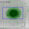 |
Fig. A.1. Hα image of NGC 4736 where green circles denote the apertures covering star-forming regions as well as the regions in between them which have Hα detection. The blue rectangular box shows the region covered by the CO map. The apertures within the blue rectangular box are used for Schmidt relation analysis. |
Appendix B: Maximum aperture-size
To determine a viable maximum aperture size we experimented on NGC 0628 which is at an intermediate distance (∼7.3 Mpc) and is almost-face-on (inclination angle ∼7°), mitigating any effect due to inclination angle. Figure B.1 shows the results of this experiment where in each panel, the y-axis shows the flux (for SFR tracers), or mass for gas data, in successive apertures of size varying from 0.6–2.0 kpc, normalised by the flux, or mass, in the smallest aperture (∼500 pc). The x-axes show the average flux/mass in the corresponding apertures. In the first four panels, we find that for each tracer (Hα, FUV, 24 μm and CO) the normalised flux/mass (solid colour line) shows the same trend, following closely the ratio of the total flux or mass (dashed colour line) for all apertures varying from 0.6–2.0 kpc. However, the corresponding plot for H I (bottom panel), shows a deviation in the trend at an aperture radius of ∼14″ (solid pink line) which corresponds to physical size of ∼1 kpc. This deviation becomes significant at physical sizes greater than ∼2 kpc. A physical size of 1.0 kpc was found suitable for two galaxies (NGC 3351 and NGC 5055) in the sample owing to their distances and inclination angles. Due to the high inclination angle of NGC 3521, a physical size of 1.0 kpc still leads to problems of under-sampling the enclosed pixels in apertures. Hence for a comparison with Liu et al. (2011) who studied Schmidt relation for this galaxy at 2.0 kpc scale, we set the aperture size for NGC 3521 to correspond to a physical size of ∼2.0 kpc. The individual results for this galaxy should be interpreted with caution due to the potential deviation in trend of H I beyond 1 kpc.
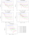 |
Fig. B.1. Flux (mass) in apertures of size varying from 0.6–2.0 kpc normalised by the flux (mass) in an aperture of size ∼500 pc compared to the average flux (mass) in the corresponding apertures. The solid colour lines show the normalised flux (mass) while the dashed colour lines show the ratio of the total flux in the apertures under study, where i and j denote the aperture radii in arcsec. These figures correspond to analysis of the galaxy NGC 0628, for which the minimum radius (8″) and maximum radius (26″) correspond to physical sizes of ∼600 pc and 2 kpc, respectively. |
Appendix C: Background subtraction on a mock galaxy
We modelled the mock galaxy (Fig. C.1) as a combination of star-forming regions, a discy exponential profile and used similar noise model properties to the real data. For simulating H II regions, we used Moffat profiles defined by I(r) = Io[1 + (r/α)2]−β where Io is the peak intensity at the centre, and α and β are related to FWHM as:  . The FWHM was set to be 2″ similar to the real data. The intensity enclosed in an aperture of radius R is given by
 ![Mathematical equation: $ I({ < }R) = \frac{\pi\alpha^2}{\beta - 1}I_{\mathrm{o}}[1 - [1+(R/\alpha)^2]^{-\beta + 1}] $](/articles/aa/full_html/2020/02/aa32467-17/aa32467-17-eq17.gif) from which aperture corrections can be readily computed. In our modelling, we experimented with two values of β = 1.5, 2.5. A Moffat profile with β = 2.5 produces a more Gaussian-like profile, while a Moffat profile with β = 1.5 produces extended outer wings, providing a better representation of the H II regions. Model flux values for the H II regions were taken from the original unsubtracted Hα image of the galaxy NGC 0628. The diffuse background exponential disc was modelled based on the effective radius of the galaxy and scaled to yield a diffuse background component of 25%. On the modelled galaxy images (β = 1.5, 2.5), as for the real data, we used the Nebulosity Filter software to estimate ab-initio the diffuse background component. We then performed aperture photometry with apertures of radii of 8″ (the same as adopted for NGC 0628) to extract fluxes in the background subtracted modelled H II regions. Aperture corrections corresponding to the two Moffat profiles were applied on the extracted fluxes, and aperture-corrected fluxes were compared with the input fluxes used to model H II regions. Figure C.2 shows comparisons of the input and output fluxes for the modelled galaxies with β = 1.5 (left panel) and β = 2.5 (right panel). The input and output fluxes lie on the expected one-to-one line (red-dashed line) expanding over two order of magnitudes.
from which aperture corrections can be readily computed. In our modelling, we experimented with two values of β = 1.5, 2.5. A Moffat profile with β = 2.5 produces a more Gaussian-like profile, while a Moffat profile with β = 1.5 produces extended outer wings, providing a better representation of the H II regions. Model flux values for the H II regions were taken from the original unsubtracted Hα image of the galaxy NGC 0628. The diffuse background exponential disc was modelled based on the effective radius of the galaxy and scaled to yield a diffuse background component of 25%. On the modelled galaxy images (β = 1.5, 2.5), as for the real data, we used the Nebulosity Filter software to estimate ab-initio the diffuse background component. We then performed aperture photometry with apertures of radii of 8″ (the same as adopted for NGC 0628) to extract fluxes in the background subtracted modelled H II regions. Aperture corrections corresponding to the two Moffat profiles were applied on the extracted fluxes, and aperture-corrected fluxes were compared with the input fluxes used to model H II regions. Figure C.2 shows comparisons of the input and output fluxes for the modelled galaxies with β = 1.5 (left panel) and β = 2.5 (right panel). The input and output fluxes lie on the expected one-to-one line (red-dashed line) expanding over two order of magnitudes.
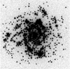 |
Fig. C.1. Mock galaxy where H II regions are modelled as Moffat profiles with β = 1.5. For more details on the modelling see the text in Appendix C. |
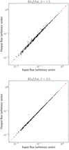 |
Fig. C.2. In both panels, x-axis shows the input fluxes to model H II regions in a mock galaxy with an underlying diffuse component and y-axis shows the fluxes in H II regions after diffuse background subtraction. In both panels, the dashed red line is the one-to-one line. H II regions are modelled as the Moffat profiles with β = 1.5 (upper panel) and β = 2.5 (lower panel). |
Appendix D: Radial profiles on unsubtracted data
Figure D.1 presents radial profiles of ΣSFR (brown curve: Hα and black curve: FUV), ΣH I (blue curve), ΣH2 (red curve), ΣH I+H2 (green curve) for all nine galaxies in the sample before subtraction of diffuse background. We do not show radial profiles of ΣH2 for r > 0.7 r25 because the radial profiles of CO intensity are found to fall below 3σ approximately after this radius (Leroy et al. 2009). The radial profiles ΣH2 (red curves) are decreasing strongly with radius in all galaxies and are closely correlated with the ΣSFR radial profiles (brown and black curves).
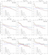 |
Fig. D.1. Radial profiles of ΣSFR (original unsubtracted data), ΣH I, ΣH2 and ΣH I+H2 for all nine galaxies in the sample. The x-axis presents the galactocentric radius normalised by r25 (bottom) and in arcsecs (top). The y-axis presents Σgas in units of M⊙ pc−2 and ΣSFR in units of 10−3 M⊙ yr−1 kpc−2 (the scale range is the same for all galaxies). ΣH2 (red curves) and ΣSFR (brown and black curves) show a similar radial falloff for all galaxies. ΣH I (blue curves) have a relatively flat radial profile, usually a deficit towards the centre and show an upper limit of ∼10 M⊙ pc−2. |
The radial profiles of ΣH I (blue curves) on the other hand show a well-defined upper limit of ∼10 M⊙ pc−2 and in general a strong depletion towards the galaxy centres. There is a relatively high surface density of molecular gas compared to atomic gas in the centre of all galaxies (r < 0.2 r25), while in the outer parts ΣH2 decreases in the regions where H I saturates. Clearly the formation and destruction of H I and H2 are interdependent and these trends presumably follow naturally from the interplay of H I, H2 and star formation. In the centres of these galaxies most of the H I is presumably in the form of H2 which is itself being used to form stars. In the outer regions, either molecular gas dissociates back to form atomic gas which suppresses star formation, or formation of molecular gas is itself low because of the lower amount of dust5 needed for molecule formation, and sufficient provision of energetic FUV photons in the extended arms of galaxies leading to further dissociation of molecular gas into atomic gas.
We note that the radial profiles of the original unsubtracted data for these galaxies have been published before by Bigiel et al. (2008), Leroy et al. (2008), and Schruba et al. (2011), though the methods adopted are slightly different in each analysis. We present them here to compare with the profiles obtained from the subtracted data presented in Fig. 4.
Appendix E: Power-law fit: weighted versus unweighted
We experimented with different methods for fitting the total gas Schmidt relation to the spatially-resolved data of NGC 0628, where no diffuse background was subtracted. These fitting methods include a standard unweighted regression, inverse unweighted regression, and maximum likelihood fits (both weighted and unweighted). The results of all the fits are shown in Fig. E.1. Previous studies have shown that calibration errors as large as 30–50% may exist on both axes owing to uncertainties on the SFR calibration and the CO-to-H2 conversion. Hence in the weighted maximum likelihood fit (solid blue line), we include a 20% calibration error on both axes in addition to the uncertainties estimated in Sect. 3.2. We test the goodness of fit from the value of the reduced-χ2 obtained. We find that the reduced-χ2 is close to unity (0.98 in this case) when additional calibration uncertainties are included in the maximum likelihood fit. Without this additional uncertainty the reduced-χ2 is much larger than one indicative of an incorrect data model. The parameters obtained from the weighted fit are similar to those derived from a maximum likelihood fit where equal weight is given to each point on both axes (solid black line). Hence based on these experiments, we decided to estimate the best-fit parameters using an equal weight maximum likelihood fit in all the analysis.
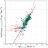 |
Fig. E.1. Different fits to the spatially-resolved total Schmidt relation for NGC 0628. Only blue points with green error bars are used for fitting. The red data points with errorbars correspond to points with S/N < 3, and have not been included in the fits. The error bars shown here include the random error and systematic error on flux measurements as explained in Sect. 3.2, but not the additional calibration error. Dashed red line: standard unweighted regression, dashed orange line: inverse weighted regression. solid black line: maximum likelihood estimate where each point on both axes is given equal weight, solid blue line: maximum likelihood estimate where 20% calibration error has been included on both axes in addition to the uncertainties estimated in Sect. 3.2, solid red line: maximum likelihood estimate where points have been weighted solely with respect to the uncertainties estimated in Sect. 3.2. |
Appendix F: Schmidt law fits to individual galaxies
Figures F.1–F.8 show the effect of inclusion and removal of diffuse background from the SFR tracers for each individual galaxy, except NGC 0628 for which the plots are shown in Fig. 5. The caption of Fig. 5 holds true for all the eight figures. Figure F.9 shows the Schmidt relation between ΣSFR and ΣH I after the diffuse background is subtracted from the SFR tracers as well as from the H I, individually for all the sample galaxies, except NGC 0628. Figure F.10 shows the total gas Schmidt relation after subtraction of diffuse background from SFR tracers and atomic gas for all galaxies except NGC 0628. See Fig. 6 for the corresponding plots of NGC 0628.
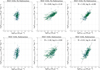 |
Fig. F.1. NGC 3184: an aperture size of 10″is adopted, which corresponds to a physical diameter of ∼520 pc for NGC 3184, at a distance of 11.1 Mpc and inclination angle of 18°. See caption of Fig. 5 for details. |
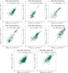 |
Fig. F.2. NGC 3351: an aperture size of 16″ is adopted, which corresponds to the physical diameter of ∼1.0 kpc at a distance of 9.33 Mpc and inclination angle of 41°. See caption of Fig. 5 for details. |
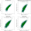 |
Fig. F.3. NGC 3521: an aperture size of 18″ is adopted, which corresponds to the physical diameter of ∼2.0 kpc at a distance of 8.03 Mpc and inclination angle of 73°. See caption of Fig. 5 for details. |
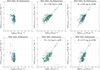 |
Fig. F.4. NGC 4736: an aperture size of 15″ is adopted, which corresponds to the physical diameter of ∼500 pc at a distance of 5.20 Mpc and inclination angle of 41°. See caption of Fig. 5 for details. |
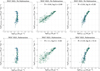 |
Fig. F.5. NGC 5055: an aperture size of 12″ is adopted, which corresponds to the physical diameter of ∼1 kpc at a distance of 7.8 Mpc and inclination angle of 59°. See caption of Fig. 5 for details. |
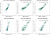 |
Fig. F.6. NGC 5194: an aperture size of 13″ is adopted, which corresponds to the physical diameter of ∼520 pc at a distance of 8.2 Mpc and inclination angle of 20°. See caption of Fig. 5 for details. |
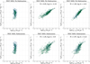 |
Fig. F.7. NGC 5457: an aperture size of 14″ is adopted, which corresponds to the physical diameter of ∼500 pc at a distance of 6.7 Mpc and inclination angle of 18°. See caption of Fig. 5 for details. |
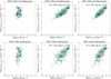 |
Fig. F.8. NGC 6946: an aperture size of 12″ is adopted, which corresponds to the physical diameter of ∼596 pc at a distance of 6.8 Mpc and inclination angle of 33°. See caption of Fig. 5 for details. |
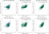 |
Fig. F.9. Spatially-resolved atomic gas Schmidt relation (ΣSFR and ΣH I (sub)). The diffuse background has been subtracted from both SFR tracers and atomic gas. |
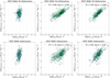 |
Fig. F.10. Spatially-resolved total gas Schmidt relation (i.e. ΣSFR and ΣH I (sub) + H2) for individual galaxies. The diffuse background has been subtracted from both SFR tracers and atomic gas. A Kroupa IMF and a constant X(CO) factor = 2.0 × 1020 cm−2 (K km s−1)−1) have been assumed. |
Appendix G: Schmidt relations using FUV
Figure G.1 shows spatially-resolved total gas Schmidt relations for all galaxies in the sample where attenuation-corrected FUV is used as SFR tracer.
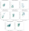 |
Fig. G.1. Spatially-resolved total gas Schmidt relation (ΣSFR and ΣH I+H2), where SFR is estimated using FUV (Eq. (5)) rather than using Hα. In each panel, blue dots with green error bars are the spatially-resolved data, and the solid black line shows the best-fit to the spatially-resolved data for all galaxies. We have assumed a Kroupa IMF and adopted a constant X(CO) factor = 2.0 × 1020 cm−2 (K km s−1)−1. Upper-left panel: no subtraction of diffuse background is done. The vertical dotted line corresponds to 10 M⊙ pc−2 around which atomic gas surface density saturates. Upper-right panel: the diffuse background is subtracted from the SFR tracers. Lower-left panel: the diffuse background is subtracted from the SFR tracers as well as from the atomic gas. Lower-right panel: the diffuse background is subtracted from the SFR tracers, HI and CO. The trend and best-coefficients of total gas Schmidt relations obtained using FUV agree with those obtained from Hα (see Fig. 8 and Table 6). |
All Tables
Percentage of diffuse background in each of the SFR tracers and atomic gas in the star-forming regions in the sample galaxies, along with the filtering scale used in Nebulosity Filter.
Comparison of parameters of Schmidt relation obtained by using different SFR tracers (Hα and FUV) by fitting data points from all galaxies.
All Figures
|
Fig. 1. Upper panel: original images of galaxy NGC 0628 before subtraction of diffuse background. Middle panel: images after subtraction of diffuse background, which show likely current star-forming regions. Lower panel: images of estimated diffuse background, showing its complex spatially varying nature. The images in a particular wavelength have the same flux scale limits. |
| In the text | |
|
Fig. 2. Left panel: HI map of NGC 5055 obtained by combining data taken in B, C and D configurations of VLA. Middle panel: HI map of NGC 5055 obtained after processing the HI map in left panel with the Nebuliser, i.e. after subtraction of diffuse background. Right panel: HI map of NGC 5055 obtained by reducing data taken in B configuration of VLA, which should not contain any diffuse background. The images obtained via the two methods (middle panel and right panel) show similar structure, and similar fraction of diffuse background (∼76% from Nebuliser and ∼78% from B-configuration map). All images have the same flux scale limits. The pixel size of the HI (B-configuration) (right panel) is 0.5 arcsec while the other two have pixel size of 2 arcsec, same as CO map. |
| In the text | |
|
Fig. 3. Comparison of attenuation-corrected ΣSFR calculated from Hα and FUV before (upper panel) and after subtraction (lower panel) of diffuse background in SFR tracers for NGC 0628. The solid black line shows the best-fit to the data and the dashed red line is the one-to-one relation between the two recipes of ΣSFR. The scaling relation does not change significantly which shows that the subtraction of diffuse background is done consistently in all SFR tracers. |
| In the text | |
|
Fig. 4. Radial profiles of ΣSFR for all nine galaxies in sample after removal of diffuse background. The x-axis presents the galactocentric radius normalised by r25 (bottom) and in arcsecs (top). The y-axis presents ΣSFR in units of 10−3 M⊙ yr−1 kpc−2 (the scaling is performed for comparison with radial plots from original unsubtracted data in Fig. D.1). The brown and black curves denote ΣSFR(Hα + 24 μm) and ΣSFR(FUV + 24 μm) respectively obtained from the data where diffuse background is subtracted from the SFR tracers. The magenta and orange curves denote ΣSFR(Hα + 24 μm) and ΣSFR(FUV + 24 μm), respectively obtained from the diffuse background maps of the SFR tracers. |
| In the text | |
|
Fig. 5. Effect of subtraction of diffuse background in SFR tracers on spatially-resolved (∼560 pc) Schmidt relations in NGC 0628. Upper panel: analysis on the images with diffuse background (no subtraction). Lower panel: analysis on the images where diffuse background is subtracted. Left panel: ΣSFR versus ΣH I, middle panel: ΣSFR versus ΣH2. Right panel: ΣSFR versus ΣH I+H2. The error bars include the random error and systematic error on the flux measurements. The solid black line in each plot denotes the best-fit line to the data where equal weight is given to each data point on both axes. N and A denote the power-law index and the star-formation efficiency. The slope of the ΣSFR versus ΣH2 and ΣSFR versus ΣH I+H2 increases after subtraction of diffuse background. We note the saturation of H I at ∼10 M⊙ pc−2. Here, we assumed a Kroupa IMF and adopted a constant X(CO) factor = 2.0 × 1020 cm−2 (K km s−1)−1. |
| In the text | |
|
Fig. 6. Effect of subtraction of diffuse background in atomic gas and SFR tracers on spatially-resolved Schmidt relations in NGC 0628. Upper panel: ΣSFR versus ΣH I. Lower panel: ΣSFR versus ΣH I+H2. See caption of Fig. 5 for details on legends. |
| In the text | |
|
Fig. 7. Spatially-resolved molecular gas Schmidt relation (ΣSFR versus ΣH2) for all sample galaxies, where the diffuse background has been subtracted from the SFR tracers. The red line is the fit obtained by averaging N (power-law indices) and log A (star-formation efficiencies) from individual galaxies (Table 4). The solid black line shows the best-fit to the spatially-resolved data for all galaxies. A Kroupa IMF and a constant X(CO) factor = 2.0 × 1020 cm−2 (K km s−1)−1 have been assumed. |
| In the text | |
|
Fig. 8. Spatially-resolved total gas Schmidt relation (ΣSFR and ΣH I+H2). In each panel, blue dots with green error bars are the spatially-resolved data, and the solid black line shows the best-fit to the spatially-resolved data for all galaxies. We have assumed a Kroupa IMF and adopted a constant X(CO) factor = 2.0 × 1020 cm−2 (K km s−1)−1. Upper-left panel: no subtraction of diffuse background is done. The vertical dotted line corresponds to 10 M⊙ pc−2 around which atomic gas surface density saturates. Upper-right panel: the diffuse background is subtracted from the SFR tracers. The solid yellow line and the dashed red line denote star-formation relation from Elmegreen 2015 (E2015) and correspond to velocity dispersion (σ) of 6 km s−1 and 11 km s−1 respectively. Lower-left panel: the diffuse background is subtracted from the SFR tracers as well as from H I. Lower-right panel: the diffuse background is subtracted from the SFR tracers, HI and CO. The solid yellow solid line on lower panels corresponds to the star-formation relation based on a dynamical model from Elmegreen (2015) obtained at a constant scale height of H = 100 pc. See text in Sect. 5.1 for further details on models. |
| In the text | |
|
Fig. 9. Comparison of the spatially-resolved total gas Schmidt relation for nine spiral galaxies in this work with the global Kennicutt–Schmidt relation of the starbursts (black stars) and spirals (yellow dots) taken from Kennicutt (1998b), low surface brightness galaxies (LSBs, orange triangles) from Wyder et al. (2009) and dwarf irregular galaxies (dIrrs, pink squares) from Roychowdhury et al. (2017). The diffuse background has been subtracted from the SFR tracers as well as from the atomic gas for the spatially-resolved data (blue dots with green error bars). These local measurements assume a Salpeter IMF and an X(CO) factor of 2.8 × 1020 cm−2 (K km s−1)−1 to match the parameters adopted in Kennicutt (1998b). The pink line represents the global Kennicutt–Schmidt relation from Kennicutt (1998b) while the solid black line is the best-fit line to the spatially-resolved data from all galaxies in this work. |
| In the text | |
|
Fig. A.1. Hα image of NGC 4736 where green circles denote the apertures covering star-forming regions as well as the regions in between them which have Hα detection. The blue rectangular box shows the region covered by the CO map. The apertures within the blue rectangular box are used for Schmidt relation analysis. |
| In the text | |
|
Fig. B.1. Flux (mass) in apertures of size varying from 0.6–2.0 kpc normalised by the flux (mass) in an aperture of size ∼500 pc compared to the average flux (mass) in the corresponding apertures. The solid colour lines show the normalised flux (mass) while the dashed colour lines show the ratio of the total flux in the apertures under study, where i and j denote the aperture radii in arcsec. These figures correspond to analysis of the galaxy NGC 0628, for which the minimum radius (8″) and maximum radius (26″) correspond to physical sizes of ∼600 pc and 2 kpc, respectively. |
| In the text | |
|
Fig. C.1. Mock galaxy where H II regions are modelled as Moffat profiles with β = 1.5. For more details on the modelling see the text in Appendix C. |
| In the text | |
|
Fig. C.2. In both panels, x-axis shows the input fluxes to model H II regions in a mock galaxy with an underlying diffuse component and y-axis shows the fluxes in H II regions after diffuse background subtraction. In both panels, the dashed red line is the one-to-one line. H II regions are modelled as the Moffat profiles with β = 1.5 (upper panel) and β = 2.5 (lower panel). |
| In the text | |
|
Fig. D.1. Radial profiles of ΣSFR (original unsubtracted data), ΣH I, ΣH2 and ΣH I+H2 for all nine galaxies in the sample. The x-axis presents the galactocentric radius normalised by r25 (bottom) and in arcsecs (top). The y-axis presents Σgas in units of M⊙ pc−2 and ΣSFR in units of 10−3 M⊙ yr−1 kpc−2 (the scale range is the same for all galaxies). ΣH2 (red curves) and ΣSFR (brown and black curves) show a similar radial falloff for all galaxies. ΣH I (blue curves) have a relatively flat radial profile, usually a deficit towards the centre and show an upper limit of ∼10 M⊙ pc−2. |
| In the text | |
|
Fig. E.1. Different fits to the spatially-resolved total Schmidt relation for NGC 0628. Only blue points with green error bars are used for fitting. The red data points with errorbars correspond to points with S/N < 3, and have not been included in the fits. The error bars shown here include the random error and systematic error on flux measurements as explained in Sect. 3.2, but not the additional calibration error. Dashed red line: standard unweighted regression, dashed orange line: inverse weighted regression. solid black line: maximum likelihood estimate where each point on both axes is given equal weight, solid blue line: maximum likelihood estimate where 20% calibration error has been included on both axes in addition to the uncertainties estimated in Sect. 3.2, solid red line: maximum likelihood estimate where points have been weighted solely with respect to the uncertainties estimated in Sect. 3.2. |
| In the text | |
|
Fig. F.1. NGC 3184: an aperture size of 10″is adopted, which corresponds to a physical diameter of ∼520 pc for NGC 3184, at a distance of 11.1 Mpc and inclination angle of 18°. See caption of Fig. 5 for details. |
| In the text | |
|
Fig. F.2. NGC 3351: an aperture size of 16″ is adopted, which corresponds to the physical diameter of ∼1.0 kpc at a distance of 9.33 Mpc and inclination angle of 41°. See caption of Fig. 5 for details. |
| In the text | |
|
Fig. F.3. NGC 3521: an aperture size of 18″ is adopted, which corresponds to the physical diameter of ∼2.0 kpc at a distance of 8.03 Mpc and inclination angle of 73°. See caption of Fig. 5 for details. |
| In the text | |
|
Fig. F.4. NGC 4736: an aperture size of 15″ is adopted, which corresponds to the physical diameter of ∼500 pc at a distance of 5.20 Mpc and inclination angle of 41°. See caption of Fig. 5 for details. |
| In the text | |
|
Fig. F.5. NGC 5055: an aperture size of 12″ is adopted, which corresponds to the physical diameter of ∼1 kpc at a distance of 7.8 Mpc and inclination angle of 59°. See caption of Fig. 5 for details. |
| In the text | |
|
Fig. F.6. NGC 5194: an aperture size of 13″ is adopted, which corresponds to the physical diameter of ∼520 pc at a distance of 8.2 Mpc and inclination angle of 20°. See caption of Fig. 5 for details. |
| In the text | |
|
Fig. F.7. NGC 5457: an aperture size of 14″ is adopted, which corresponds to the physical diameter of ∼500 pc at a distance of 6.7 Mpc and inclination angle of 18°. See caption of Fig. 5 for details. |
| In the text | |
|
Fig. F.8. NGC 6946: an aperture size of 12″ is adopted, which corresponds to the physical diameter of ∼596 pc at a distance of 6.8 Mpc and inclination angle of 33°. See caption of Fig. 5 for details. |
| In the text | |
|
Fig. F.9. Spatially-resolved atomic gas Schmidt relation (ΣSFR and ΣH I (sub)). The diffuse background has been subtracted from both SFR tracers and atomic gas. |
| In the text | |
|
Fig. F.10. Spatially-resolved total gas Schmidt relation (i.e. ΣSFR and ΣH I (sub) + H2) for individual galaxies. The diffuse background has been subtracted from both SFR tracers and atomic gas. A Kroupa IMF and a constant X(CO) factor = 2.0 × 1020 cm−2 (K km s−1)−1) have been assumed. |
| In the text | |
|
Fig. G.1. Spatially-resolved total gas Schmidt relation (ΣSFR and ΣH I+H2), where SFR is estimated using FUV (Eq. (5)) rather than using Hα. In each panel, blue dots with green error bars are the spatially-resolved data, and the solid black line shows the best-fit to the spatially-resolved data for all galaxies. We have assumed a Kroupa IMF and adopted a constant X(CO) factor = 2.0 × 1020 cm−2 (K km s−1)−1. Upper-left panel: no subtraction of diffuse background is done. The vertical dotted line corresponds to 10 M⊙ pc−2 around which atomic gas surface density saturates. Upper-right panel: the diffuse background is subtracted from the SFR tracers. Lower-left panel: the diffuse background is subtracted from the SFR tracers as well as from the atomic gas. Lower-right panel: the diffuse background is subtracted from the SFR tracers, HI and CO. The trend and best-coefficients of total gas Schmidt relations obtained using FUV agree with those obtained from Hα (see Fig. 8 and Table 6). |
| In the text | |
Current usage metrics show cumulative count of Article Views (full-text article views including HTML views, PDF and ePub downloads, according to the available data) and Abstracts Views on Vision4Press platform.
Data correspond to usage on the plateform after 2015. The current usage metrics is available 48-96 hours after online publication and is updated daily on week days.
Initial download of the metrics may take a while.