| Issue |
A&A
Volume 631, November 2019
|
|
|---|---|---|
| Article Number | A177 | |
| Number of page(s) | 21 | |
| Section | Stellar structure and evolution | |
| DOI | https://doi.org/10.1051/0004-6361/201936501 | |
| Published online | 19 November 2019 | |
Overview of non-transient γ-ray binaries and prospects for the Cherenkov Telescope Array
1
School of Physical Sciences and CfAR, Dublin City University, Dublin 9, Ireland
e-mail: This email address is being protected from spambots. You need JavaScript enabled to view it.
2
Dublin Institute for Advanced Studies, 31 Fitzwilliam Place, Dublin 2, Ireland
3
Institut für Astronomie und Astrophysik Tübingen, Universität Tübingen, Sand 1, 72076 Tübingen, Germany
4
INAF – IASF Milano, Via Alfonso Corti 12, 20133 Milano, Italy
5
INAF – Osservatorio Astronomico di Brera, Via E. Bianchi 46, 23807 Merate, Italy
6
Unitat de Física de les Radiacions, Departament de Física, and CERES-IEEC, Universitat Autònoma de Barcelona, 08193 Bellaterra, Spain
7
Max-Planck-Institut für Physik, 80805 München, Germany
8
INAF – IAPS Roma, Italy
9
ISDC, University of Geneva, Switzerland
10
Astronomical Observatory of Taras Shevchenko National University of Kyiv, 3 Observatorna str. Kyiv, 04053, Ukraine
11
University of the Free State Department of Physics, PO Box 339, 9300 Bloemfontein, South Africa
12
Institut de Ciències del Cosmos (ICCUB), Universitat de Barcelona, IEEC-UB, Martí i Franquès 1, 08028 Barcelona, Spain
13
Dept of Physics and Astronomy, University of Manitoba, Winnipeg R3T 2N2, Canada
14
Unidad de Partículas y Cosmología (UPARCOS), Universidad Complutense, 28040 Madrid, Spain
15
EPS Jaén, Universidad de Jaén, Campus Las Lagunillas s/n, 23071 Jaén, Spain
16
Escola de Artes, Ciências e Humanidades, Universidade de São Paulo, Rua Arlindo Bettio 1000, 03828-000 São Paulo, Brazil
Received:
13
August
2019
Accepted:
22
September
2019
Abstract
Aims. Despite recent progress in the field, there are still many open questions regarding γ-ray binaries. In this paper we provide an overview of non-transient γ-ray binaries and discuss how observations with the Cherenkov Telescope Array (CTA) will contribute to their study.
Methods. We simulated the spectral behaviour of the non-transient γ-ray binaries using archival observations as a reference. With this we tested the CTA capability to measure the spectral parameters of the sources and detect variability on various timescales.
Results. We review the known properties of γ-ray binaries and the theoretical models that have been used to describe their spectral and timing characteristics. We show that the CTA is capable of studying these sources on timescales comparable to their characteristic variability timescales. For most of the binaries, the unprecedented sensitivity of the CTA will allow studying the spectral evolution on a timescale as short as 30 min. This will enable a direct comparison of the TeV and lower energy (radio to GeV) properties of these sources from simultaneous observations. We also review the source-specific questions that can be addressed with these high-accuracy CTA measurements.
Key words: gamma-rays: stars / gamma-rays: general / acceleration of particles / methods: observational / binaries: general
© ESO 2019
1. Introduction
γ-ray binaries are a subclass of high-mass binary systems whose energy spectrum peaks at high energies (HE, E ≳ 100 MeV) and extends to very high energy (VHE, E ≳ 100 GeV) γ-rays. In these systems a compact object (neutron star, NS, or a black hole, BH) orbits a young and massive star of either O or B type.
While high-mass binaries represent a substantial fraction of the Galactic X-ray sources that are detected above 2 keV (e.g. Grimm et al. 2002), fewer than ten binaries were detected in the γ-ray band by the current generation of Cherenkov telescopes, such as Major Atmospheric Gamma Imaging Cherenkov Telescopes (MAGIC; Aleksić et al. 2012a), Very Energetic Radiation Imaging Telescope Array System (VERITAS; Park & VERITAS Collaboration 2015), and High Energy Stereoscopic System (H.E.S.S.; Aharonian et al. 2006). Therefore γ-ray binaries represent a relatively new and unexplored class of astrophysical objects.
Of all the binary systems that are regularly observed at TeV energies, the nature of compact objects is only firmly established for two systems, PSR B1259−63 and PSR J2032+4127. In PSR B1259−63, a 43 ms radio pulsar orbits a Be star on a highly eccentric 3.4 yr orbit. Radio pulsations from the source are detected along most of the orbit, except for a brief period near periastron. The second source, which also contains a pulsar, PSR J2032+4127, has an even longer orbital period of about 50 yr (Lyne et al. 2015; Ho et al. 2017), and TeV emission was detected from this system by VERITAS and MAGIC as the pulsar approached its periastron in September 2017 (VERITAS & MAGIC Collaborations 2017).
All other known systems are more compact, and the nature of their compact object is so far unknown. It is possible that these systems harbour radio pulsars as well, but the optical depth due to the stellar wind outflow is too high to detect the radio signal that originates close to the pulsar (the so-called hidden pulsar model, see e.g. Zdziarski et al. 2010). Alternatively, it is possible that some of these systems harbour a BH or an accreting NS (the microquasar model, Mirabel & Rodríguez 1998).
Of the accretion-powered γ-ray binaries that likely contain a BH, the highest energy emission that has so far been regularly observed comes from Cyg X-1 and Cyg X-3 and is detected with AGILE and the Fermi Large Area Telescope (Fermi-LAT; e.g. Tavani et al. 2009a; Sabatini et al. 2010; Bodaghee et al. 2013; Malyshev et al. 2013). Cyg X-1 is detected up to about 10 GeV in the hard state (Zanin et al. 2016; Zdziarski et al. 2017), and Cyg X-3 is detected up to about 10 GeV during flares that mostly occur when the source is in the soft state (Zdziarski et al. 2018). In 2006, the MAGIC telescope has also reported marginal detection of a TeV flare from Cyg X-1 at a 3.2σ confidence level. This coincides with an X-ray flare seen by RXTE, Swift, and INTEGRAL (Albert et al. 2007). We therefore currently have evidence that accreting sources can accelerate particles only during some very specific states, and we need to study the persistent γ-ray binaries in detail to unveil their ability to steadily accelerate particles (at least at given orbital phases). Recently, the microquasar SS433 was also detected by Fermi-LAT and HAWC (Bordas et al. 2015; Abeysekara et al. 2018). The persistent emission reported by HAWC is localised to structures in the lobes, far from the centre of the system. This implies a very different emission scenario to the other systems.
In addition to the γ-ray binaries that contain a compact object, HE and VHE γ-rays have also been detected from colliding-wind binaries (CWB). A CWB is a binary star system consisting of two non-compact massive stars that emit powerful stellar winds, with high mass-loss rates and high wind velocities. The collision of the winds produces two strong shock fronts, one for each wind. They surround a shock region of compressed and heated plasma, where particles are accelerated to VHEs (Eichler & Usov 1993). To date, only one CWB has a confirmed detection at VHE: η Carinae (η Car).
The family of γ-ray binaries can be extended through follow-up observations in the next years based on indications from lower energy bands. In particular, binaries with pulsars orbiting Be or O stars are likely to provide a noticeable addition to the γ-ray binary list. Similarly, BH and Be star binaries can also be considered good candidates for the γ-ray binary family (Williams et al. 2010; Munar-Adrover et al. 2016), although only one system, MWC 656, is known so far (Casares et al. 2014). Other alternative search efforts have focused on multi-wavelength cross-identification that explores the possible association of luminous early-type stars with GeV γ-ray sources (mainly) detected by Fermi-LAT (McSwain et al. 2013; Martí et al. 2017). Still, Dubus et al. (2017) recently carried out a synthetic population simulation and estimated that fewer than 230 systems exist inside the Milky Way.
In recent years, γ-ray binaries have already been the subject of numerous observational campaigns and theoretical studies (e.g. Dubus 2013), which strongly indicate that the high-energy emission from these systems is primarily powered by the outflow from the compact object. However, due to the limited sensitivity of the current generation of instruments, the nature of the compact object (NS or BH) and the details of the particle acceleration, with efficiency sometimes close to the theoretical limit (e.g. Johnson et al. 2018), remain unknown in most of the systems (e.g. Paredes & Bordas 2019).
Existing data have shown that in some systems such as LS 5039 and LS I +61° 303, the observed HE and VHE emission are separate components that are generated at different places (e.g. Zabalza et al. 2013, and references therein). A proper modelling of these double-component spectra requires time-resolved spectroscopy throughout the binary orbit. In addition, γ-ray binaries are known to be variable on timescales as short as hours, minutes, and even tens of seconds, as observed in X-ray and HE bands (e.g. Chernyakova et al. 2009; Smith et al. 2009; Johnson et al. 2018). At the same time, with the current generation of VHE telescopes, observations can only provide information that is averaged over several days even for the brightest binaries. The possibility of studying the broad-band spectral variability on a characteristic timescales is crucial for an unambiguous modelling.
In the next decade this situation may change with the deployment of the next-generation VHE telescope, the Cherenkov Telescope Array (CTA) observatory.
The CTA will be composed of two sites, one in the Northern (La Palma, Canary Islands) and one in the Southern Hemisphere (Paranal Observatory, Chile), which will enable observations to cover the entire Galactic plane and a large fraction of the extra-galactic sky (see e.g. CTA Consortium 2017). The array will include three different telescope sizes to maximise the energy range of the instrument (from 20 GeV to more than 300 TeV). With more than 100 telescopes in the Northern and Southern Hemispheres, the CTA will be the largest ground-based γ-ray observatory in the world. The CTA will be 5–20 times more sensitive (depending on the energy) than the current generation of ground-based γ-ray detectors (CTA Consortium 2019). It is foreseen that CTA will make a breakthrough in many areas, including the study of γ-ray binaries. Beyond detailed studies of the known binaries, the CTA is foreseen to discover new sources, enlarging the population. Dubus et al. (2017) has estimated that four new γ-ray binaries can be expected to be detected in the first two years of the CTA Galactic Plane survey.
The aim of this paper is to estimate the potential of the CTA for observations of known γ-ray binary systems. The text is organised as follows. In Sect. 2 we outline the source selection and CTA simulation setup. Sections 3 and 4 present the results of simulations for specific binary system types. Finally, in Sect. 5 we briefly summarise and discuss our results.
2. Simulations
All the simulations that are reported in this paper were performed with the ctools analysis package1 (Knödlseder et al. 2016, v 1.5), together with the prod3b-v1 set of instrument response functions (IRFs2) for both the northern (La Palma) and southern (Paranal) CTA sites. In prod3b-v1 IRFs only exist for zenith angles of 20 and 40°. To select the correct response function, we used a simple relation between the minimum zenith angle of the source (mza) and declination (Dec) and the latitude (lat) of the site: mza = |lat − Dec|. For example, for La Palma (lat = +29°), HESS J0632+057 has an mza = 23°. Thus the 20° IRF is the most appropriate. For the southern site (Paranal, lat = −25°), HESS J0632+057 has a minimal zenith angle of 31°, and we chose the 40° IRF.
In the analysis, we simulated the data with ctobssim and fitted simulated event files with ctlike using a maximum likelihood method. To simulate the event file, we used all sources listed in TeVCat3 within a circle of 5° around the source position. In addition, we included the instrumental background and the Galactic diffuse γ-ray emission in the model of the region surrounding the simulated source4. All errors presented in the paper are the statistical errors at a 1σ confidence level.
3. γ-ray binaries with a compact source
This section is devoted to an overview of the non-transient, point-like, γ-ray binary sources that all consist of an O- or B/Be-type star and a compact object (pulsar or BH). The specific sources studied here are listed in Table 1. PSR J2032+4127 is not included because with a ≈50 yr orbital period, it is unlikely that the next periastron passage will be observed with the CTA. Very recently, while this paper was under revision, a new γ-ray binary candidate, 4FGL J1405.1−6119, was discovered (Corbet et al. 2019). The TeV properties of the source are currently not known and we therefore do not discuss this source here either.
Properties of γ-ray binaries with a compact source.
The VHE emission of all the γ-ray binaries is well described by a power law with an exponential high-energy cut-off. As was mentioned in the introduction, current VHE observations are not sensitive enough to follow the details of the spectral evolution of these systems on their characteristic timescales.
In order to test the future capabilities of the CTA, we calculated the predicted errors on the spectral parameters for different characteristic fluxes on 30 min and 5 h timescales in the 1–100 TeV energy range. To do this, we considered 100 random realisations of the region surrounding the binary. For each simulation we used a power-law spectral shape and assumed flux and spectral slope values that are typical for the simulated γ-ray binary. The uncertainties are defined as a standard deviation of the distribution of best-fit values. The results are shown in the top and middle panels of Fig. 1. While for most systems the spectral shape above 1 TeV nicely follows a power law, it is not yet clear at which energy we should expect a cut-off. In order to estimate the maximum energy up to which the CTA will be able to firmly detect a cut-off, we fitted event data (simulated for a power-law spectral energy distribution) with a cut-off power-law model. This was repeated 1000 times for different data realisations. From the obtained distribution of best-fit cut-off values we found a value above which 95% of all cut-off values are located. This corresponds to the 95% upper limit on the cut-off energy, that is, if the cut-off is detected by the CTA at energies lower than this, we can be confident that it is real. The resulting 95% confidence values for sources with fluxes F(> 1 TeV) < 1.5 × 10⁻¹² ph cm−2 s−1 are shown in the bottom panel of Fig. 1. For sources with higher fluxes, the resulting value of the cut-off is close to 100 TeV. The spectrum of PSR B1259−63 is much softer (Γ ≈ 2.9) than those of other binaries (Γ ≈ 2.3), which results in a lower value of the cut-off energy that can be detected by the CTA.
 |
Fig. 1. Summary of the simulations we performed for the different binaries for various exposure times and telescope configurations. Left and right panels: south and north sites, respectively. Exposure time is shown with colours: blue corresponds to 30 min and red to 5 h. In this figure, we show the dependence of the relative flux error (top panel), spectral slope error (middle panel), and maximum energy up to which a cut-off can be excluded (bottom panel). |
We furthermore confirmed that for a given flux and exposure time, the error on the slope has a weak dependence on the slope value. Figure 2 illustrates the slope uncertainty (shown with colour) as a function of the slope and the 1–10 TeV flux level for a 5 h observation of the point-like source located at the position of PSR B1259−63.
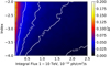 |
Fig. 2. Uncertainty on the slope (colour bar) as a function of the slope value and the flux in the 1 − 10 TeV energy range for 5 h observations of a point-like source at the position of PSR B1259−63. White lines illustrate the levels of constant slope uncertainty. |
Lastly, in this section we present an overview of what is known about each source listed in Table 1. We discuss the questions that can be answered with the new data measured with the precision shown in Fig. 1, and present results of other simulations specific to each individual case.
3.1. PSR B1259−63
3.1.1. Source properties
PSR B1259−63 was first discovered as part of a search for short-period pulsars with the Parkes 64 m telescopes (Johnston et al. 1992a), and was the first radio pulsar discovered in orbit around a massive non-degenerate star, the Be star LS 2883 (Johnston et al. 1992b). Long-term monitoring of the pulsar has allowed for a very accurate determination of the binary orbit and reveals that PSR B1259−63 is on a highly eccentric 3.4 yr orbit (Shannon et al. 2014, and references therein).
Radio observations around periastron show an increase and variability in the dispersion measurement of the pulsed signal as the pulsar passes into the stellar wind (e.g. Johnston et al. 2001). This is followed by an eclipse of the pulsed signal from ≈16 days before until ≈16 days after periastron, accompanied by the detection of unpulsed radio emission (Johnston et al. 2005, and references therein). The unpulsed emission shows a double-peak structure, reaching a maximum around the time of the start and end of the pulsar eclipse, although the shape varies between the periastron passages (e.g. Johnston et al. 2005). The unpulsed emission originates from the extended pulsar wind nebula, which is shown to extend beyond the binary by observations with the Australian Long Baseline Array (Moldón et al. 2011).
The best optical analysis of the optical companion, LS 2883, comes from high-resolution spectroscopic observations with the UVES/VLT (Negueruela et al. 2011). It is a rapidly rotating O9.5Ve star with an oblate shape and a temperature gradient from the equator to the poles. The star is wider and cooler at the equator (Req ≈ 9.7 R⊙; Teff, eq ≈ 27 500 K), and narrower and hotter at the poles (Rpol ≈ 8.1 R⊙; Teff, pol ≈ 34 000 K). The Be nature of the star is clear from the strong emission lines that are observed from the source, which originate from the out-flowing circumstellar disc (Johnston et al. 1992b, 1994; Negueruela et al. 2011). The disc is believed to be tilted relative to the orbital plane (e.g. Wex et al. 1998), with the pulsar crossing the disc plane twice per orbit. Observations have shown that the circumstellar disc is variable around periastron, with the strength of the Hα line increasing until after periastron, as well as changes in the symmetry of the double-peaked He I line (Chernyakova et al. 2014, 2015; van Soelen et al. 2016).
After first being detected at X-ray energies with ROSAT (Cominsky et al. 1994), observations around periastron have shown a remarkable similarity during different periastron passages. X-ray observations folded over multiple epochs show that the X-ray flux peaks before and after periastron, at around the same time as the pulsed radio emission becomes eclipsed (e.g. Chernyakova et al. 2015, and references therein). This is interpreted as being associated with the time the pulsar passes through the plane of the circumstellar disc. Observations around the 2014 periastron passage also revealed that the rate at which the flux decreased after the second maximum (≈20 d after periastron) slowed down and plateaued around 30 days after periastron, at the time when the GeV γ-ray emission began to increase rapidly. Extended X-ray emission has also been detected around PSR B1259−63, with an extended structure flowing away from the binary; this is suggested to be a part of the circumstellar disc that is ejected from the system and begins to become accelerated outwards by the pulsar wind (Pavlov et al. 2011, 2015).
While not detected by COMPTEL and EGRET (Tavani et al. 1996), PSR B1259−63 has subsequently been detected at GeV and TeV γ-ray energies with Fermi-LAT and H.E.S.S. The H.E.S.S. telescope has reported on observations of the source over the 2004, 2007, 2010, and 2014 periastron passages (Aharonian et al. 2005a, 2009; H.E.S.S. Collaboration 2013; Romoli et al. 2017). The combined light curves over multiple epochs are beginning to show an indication of a double-hump structure around periastron, with a dip at periastron. This is similar to what is observed at X-ray energies. The observations at GeV energies with Fermi-LAT show a very different result. During the 2011 periastron passage, a very faint detection was reported around periastron, but about 30 days after periastron, a rapid brightening (flare) with a luminosity approaching that of the pulsar spin-down luminosity was observed (Tam et al. 2011; Abdo et al. 2011). This occurred at a time when the multi-wavelength emission decreased, and a flare at this period was not expected. Observations around the following periastron, in 2014, had a substantially shorter exposure before the flare and no emission was detected before or at periastron. While the flux started to increase at around the same orbital phase, the emission peaked later and was fainter than during 2011 (Tam et al. 2015; Caliandro et al. 2015). The most recent periastron passage in 2017 has also shown a different light curve: while no γ-ray flare was reported 26–43 days after periastron (Zhou et al. 2017), a rapid flare was detected at 70 days after periastron, during a period when GeV emission was previously not detected (Johnson et al. 2017). In addition, rapid ≈3 h flares in GeV and changing UV flux have been reported during the last periastron passage (Tam et al. 2018). Detailed analysis of the short timescale variability of the source by Johnson et al. (2018) revealed even shorter substructures on a timescale of ≈10 min. The energy released during these short flares significantly exceeds the total spin-down luminosity. This demonstrates a clear variability of the emission on very different timescales from as short as few minutes up to orbit-to-orbit variability.
3.1.2. Prospects for CTA observations
The TeV γ-ray emission from PSR B1259−63 has been detected from around 100 days before until 100 days after periastron, with the next periastron occurring on 2021 February 9. The ≈3.4 yr orbital period makes observations more challenging because orbit-to-orbit variation studies must take place over long time periods. Despite this, the improved sensitivity of the CTA observations around the next periastron passages can be used to test different models and better constrain the theoretical models of this source. This may include investigating the degree of gamma-gamma absorption around periastron, searching for connections to the GeV flare, and constraining the shape of the light curve near the disc crossings.
The double-hump shape of the TeV light curve around periastron has for instance been attributed to more efficient particle acceleration during the disc crossing (Takata et al. 2012), hadronic interactions in the disc (Neronov & Chernyakova 2007), time-dependent adiabatic losses modified by the disc (Kerschhaggl 2011), and increased gamma-gamma absorption around periastron (Sushch & van Soelen 2017). Gamma-gamma absorption of the TeV photons should be highest a few days before periastron, and if TeV γ-rays are produced near the pulsar location, stellar and disc photons should decrease the flux above 1 TeV, harden the photon index, and vary the low-energy cut-off (Sushch & van Soelen 2017). The simulated light curve for PSR B1259−63 is shown in Fig. 1 for 30 min observations. These measurable limits will help to place better constraints on the level of γγ absorption in the system.
The second question the CTA can start to answer is whether there is any indication at TeV energies of a connection to the GeV flare. The H.E.S.S. observations around the 2010 periastron passage showed no TeV flare at the time of the Fermi flare (H.E.S.S. Collaboration 2013), and similarly, no multi-wavelength flare has been detected. However, X-ray observations around the 2014 periastron passage showed a change in the rate at which the flux decreased (Chernyakova et al. 2015). Observations with the CTA around periastron will allow us to search for a similar effect. This will be an important constraint on the underlying emission mechanism.
Finally, the improved sensitivity of the CTA will enable a more detailed investigation of the shape of the light curve around the periods of the disc crossings. This is an important comparison to make to models that predict various shapes around these periods, such as Kerschhaggl (2011) and Neronov & Chernyakova (2007).
To illustrate this point, we simulated the light curve of the source around periastron. For this we assumed a constant slope with Γ = 2.9 and modulated the flux above 1 TeV according to the H.E.S.S. observations reported by Romoli et al. (2017). Fig. 3 illustrates that even 30 min exposures will be enough for the CTA to measure the profile with a high accuracy.
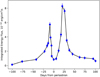 |
Fig. 3. Simulated light curve above 1 TeV of PSR B1259−63 around periastron. Each point has a 30 min exposure. |
3.2. LS I +61° 303
3.2.1. Source properties
The srouce LS I +61° 303 was first discovered as a bright γ-ray source by the Cos B satellite (Hermsen et al. 1977). Shortly after the discovery, it was realised that this source was also a highly variable radio source (Gregory & Taylor 1978) and was associated with the optical source LS I +61° 303, a young, rapidly rotating, 10–15 M⊙ B0 Ve star (Gregory et al. 1979). A young pulsar was at first suggested to be responsible for the observed radio emission (Maraschi & Treves 1981), but no pulsations have ever been detected, despite intensive searches (e.g. Sidoli et al. 2006).
Massi et al. (2017) studied the correlation between the X-ray luminosity and the X-ray spectral slope in LS I +61° 303 and found a good agreement with that of moderate-luminosity BHs. Along with the quasi-periodic oscillations observed from this system both in radio and X-rays (e.g. Nösel et al. 2018), this supports a microquasar scenario for LS I +61° 303. However, in this case, it is the only known microquasar that exhibits a regular behaviour, does not demonstrate transitions between various spectral states, and lacks a spectral break up to hard γ-rays. A magnetar-like short burst caught from the source supports the identification of the compact object in LS I +61° 303 with a NS (Barthelmy et al. 2008; Torres et al. 2012).
Radial velocity measurements of the absorption lines of the primary (Casares et al. 2005; Aragona et al. 2009) showed that LS I +61° 303 is on an elliptical (e = 0.537 ± 0.34) orbit. The orbital period of LS I +61° 303 was found to be P ≈ 26.5 d from radio observations (Gregory 2002). A strong orbital modulation in LS I +61° 303 is also observed in the optical to infrared (Mendelson & Mazeh 1989; Paredes et al. 1994), X-ray (Paredes et al. 1997), hard X-ray (Zhang et al. 2010), and HE/VHE γ-ray (Abdo et al. 2009; Albert et al. 2009) domains. In the optical band, the orbital period signature is evident not only in the broad-band photometry, but also in the spectral properties of the Hα emission line (Zamanov et al. 1999). Because of the uncertainty in the inclination of the system, the nature of the compact object remains unclear, and it can be either a NS or a stellar-mass BH (Casares et al. 2005).
In radio, LS I +61° 303 was intensively monitored at GHz frequencies for many years (e.g. Ray et al. 1997; Massi et al. 2015). The radio light curve displays periodic outbursts whose position and amplitude changed from one orbit to the next. A Bayesian analysis of radio data allowed Gregory (2002) to establish a super-orbital periodic modulation of the phase and amplitude of these outbursts with a period of Pso = 1667 ± 8 days. This modulation has also been observed in X-rays (Chernyakova et al. 2012; Li et al. 2014) and γ-rays (Ackermann et al. 2013; Ahnen et al. 2016; Xing et al. 2017). It has been suggested that the super-orbital periodicity can depend on the Be star disc, either due to a non-axisymmetric structure rotating with a period of 1667 days (Xing et al. 2017), or because of a quasi-cyclic build-up and decay of the Be decretion disc (Negueruela et al. 2001; Ackermann et al. 2013; Chernyakova et al. 2017). Another possible scenario for the super-orbital modulation is related to the precession of the Be star disc (Saha et al. 2016) or periodic Doppler-boosting effects of a precessing jet (Massi & Torricelli-Ciamponi 2016).
The precessing jet model is based on high-resolution radio observations suggesting a double-sided jet (Massi et al. 1993, 2004; Paredes et al. 1998). The precession period in this model is about 26.9 days, which is very close to the orbital period. In this case the observed super-orbital variability is explained as a beat period of the orbital and precession periods (Massi & Jaron 2013).
At GeV energies, LS I +61° 303 was unambiguously detected by Fermi-LAT (Abdo et al. 2009) through its flux modulation at the orbital period. The Fermi-LAT light curve shows a broader peak after periastron and a smaller peak just before apastron (Jaron & Massi 2014). The peak at apastron is affected by the same orbital shift as the radio outbursts and varies on the super-orbital timescale, leading to a decline in the orbital flux modulation as the two peaks merge.
A long-term investigation of Fermi-LAT data by Saha et al. (2016) showed the orbital spectral variability of the source. The observed spectrum is consistent with an exponential cut-off power law with a cut-off at 6–30 GeV for different orbital states of the system. The excess above the spectral cut-off is part of a second emission component that is dominant at the TeV domain (Hadasch et al. 2012; Saha et al. 2016).
Detected at TeV energies by MAGIC (Albert et al. 2006) and by VERITAS (Acciari et al. 2008), the VHE emission from LS I +61° 303 shows a modulation consistent with the orbital period (Albert et al. 2009) with the flux peaking at apastron. A decade-long VERITAS observation of LS I +61° 303 allowed TeV emission to be detect from the system throughout the entire orbit, with the integral flux above 300 GeV varying in the range (3 − 7)×10−12 cm−2 s−1. The VHE emission is well described by a simple power-law spectrum, with a photon index of Γ = 2.63 ± 0.06 near apastron and Γ = 2.81 ± 0.16 near periastron (Kar & VERITAS Collaboration 2017).
Similar to other wavelengths, the TeV curve varies from orbit to orbit. MAGIC observations during 2009–2010 caught LS I +61° 303 in a low state, with the TeV flux about an order of magnitude lower than was previously detected at the same orbital phase (Aleksić et al. 2012b).
Long-term multi-wavelength monitoring of LS I +61° 303 indicates a correlation between the X-ray (XMM-Newton and Swift/XRT) and TeV (MAGIC and VERITAS) data sets. At the same time, GeV emission shows no correlation with the TeV emission. Along with the spectral cut-off at GeV energies, this implies that the GeV and TeV γ-rays originate from different particle populations (Anderhub et al. 2009; Aliu et al. 2013; Kar & VERITAS Collaboration 2015).
3.2.2. Prospects for CTA observations
A correlation of VHE and X-ray emission might indicate that in this source the synchrotron emission that is visible at X-rays is due to the same electrons that produce the TeV emission by inverse Compton scattering of stellar photons. However, while X-ray variability on timescales of thousands of seconds is known from the source (Sidoli et al. 2006), MAGIC and VERITAS observations require much longer exposure times, making it difficult to clearly compare the spectral behaviour at different energies. The sensitivity of the CTA is crucial for detecting spectral variability on comparable timescales at X-rays and VHE energies.
We studied the capabilities of the CTA to unambiguously detect spectral variability of LS I +61° 303 on different timescales by performing a series of simulations that we based on existing observations. It has been observed that the spectrum of the TeV emission varies between the low and the high state. For our simulations we chose F(E > 1 TeV) = 2.6 × 10⁻¹² cm−2 s−1 for the high state and F(E > 1 TeV) = 1.2 × 10⁻¹² cm−2 s−1 for the low state. We assumed a power-law model to describe the source and used different spectral slopes to determine whether CTA would be able to distinguish between them. The spectral slopes that were chosen were Γ = 2.4, 2.7, and 3.0, in agreement with MAGIC and VERITAS observations. Simulations of both 30 min and 5 h exposure times where performed for each set of parameters. Each combination was simulated 500 times to ensure enough statistics. In the analysis of each realisation, the normalisation and spectral index were kept as free parameters.
Similarly to the simulations presented in Fig. 2, we found that the uncertainty on the spectral slope has a weak dependence on the slope value. A 5 h observation is enough to determine the slope with an accuracy better than 0.1 (see Figs. 1 and 4).
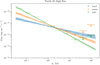 |
Fig. 4. Simulated spectra of LS I +61° 303 for 5 h observation. The three different spectral slopes are shown. Solid lines represent the power-law spectral fit. The butterfly represents the 1σ uncertainty in the fit. |
To determine the capability of the CTA to detect a VHE cut-off in LS I +61° 303, we simulated a 5 h observation with a power-law spectral model and fit the data with an exponential cut-off power law. The resulting values are shown in Fig. 1.
Finally, we studied the orbital variability of the source. We took the light curve above 400 GeV obtained by Albert et al. (2009) and modelled it with 27 bins (see Fig. 5) to study the inter-night variability of the source. We simulated the source with a power-law spectrum with a photon index Γ = 2.7. In the reconstruction the photon index and the normalisation were left free to vary. We performed 100 realisations for each orbital bin for 30 min and 5 h exposures. In this analysis we assumed a much lower value for the flux in the low state (orbital phases between 0.2 and 0.4) of about 10−14 cm−2 s−1. The resulting uncertainties for the relative flux and slope are summarised in Fig. 5. All uncertainties are statistical only at a 1σ confidence level and are below 10% for the integral flux in the high state, with the photon index uncertainty below 0.1 even for a 30 min exposure. In the low state the source is barely detected even with a 5 h exposure. The upper limits we show correspond to the 2σ confidence level. This simulation shows that if the flux of the source is above ≈10−13 cm−2 s−1, the CTA will be able to detect inter-night variability of the source at a 10% level. This precision will allow studying the superorbital variability of the orbital profile and comparing it to other energy bands. In the high state it will be possible to study the variability of the source at a 30 min timescale. This is comparable to what is observed in X-ray data (see e.g. Chernyakova et al. 2017).
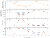 |
Fig. 5. Upper panel: original orbital light curve of LS I +61° 303 as observed by MAGIC (Albert et al. 2009). Next panel: simulated orbital light curve at E > 1 TeV, where the green line shows the simulated flux and the arrows represent 2σ upper limits. Third panel: relative uncertainty of the simulated flux. Bottom panel: uncertainty in the simulated photon index. In all panels the exposure time is shown with colours: blue corresponds to 30 min and red to 5 h. |
3.3. LS 5039
3.3.1. Source properties
LS 5039 has the shortest orbital period thus far of all known γ-ray binaries (3.9 d, see Table 1). It is also known as V497 Sct, based on ROSAT X-ray data. Motch et al. (1997) first reported it as a high-mass X-ray binary. Its peculiar nature as a persistent non-thermal radio emitter was soon revealed after the detection of a bright radio counterpart with the Very Large Array (VLA) by Martí et al. (1998). This has anticipated the capability of the system to accelerate electrons to relativistic speeds. Follow-up images obtained with very long baseline interferometry (VLBI) resolved the radio emission into elongated features, and as a result, LS 5039 was interpreted as a new microquasar system (Paredes et al. 2000). Moreover, at the same time, it was also tentatively associated with the EGRET γ-ray source 3EG J1824−1514. The confirmation of LS 5039 as an unambiguous (> 100 GeV) γ-ray source was finally obtained with H.E.S.S. (Aharonian et al. 2005b).
During the 20 yr since its discovery, the physical picture of LS 5039 has generally evolved from the microquasar scenario to a binary system hosting a young non-accreting NS interacting with the wind of a massive O-type stellar companion (see e.g. Dubus 2013 and references therein). This is strongly supported by VLBI observations of periodic changes in the radio morphology (Moldón et al. 2012), although no radio pulsations have been reported so far.
At different photon energies, the shape of the LS 5039 light curve varies, as confirmed in the most recent multi-wavelength studies using Suzaku, INTEGRAL, COMPTEL, Fermi-LAT, and H.E.S.S. data (Chang et al. 2016, and references therein). The X-ray, soft γ-ray (up to 70 MeV), and TeV emission peak around inferior conjunction after the apastron passage. In contrast, γ-rays in the 0.1–3 GeV energy range anti-correlate and have a peak near the superior conjunction soon after the periastron passage. No clear orbital modulation is apparent in the 3–20 GeV band. This dichotomy suggests a highly relativistic particle population that accounts for both X-ray/soft γ-ray and TeV emission mainly by synchrotron and anisotropic inverse Compton (IC) scattering of stellar photons, respectively. The GeV γ-ray peak would arise when TeV photons (of an IC origin) are absorbed through pair production as the NS approaches its O-type companion, and further enhances the GeV emission through cascading effects. Variable adiabatic cooling and Doppler boosting are other effects proposed to play an important role when trying to understand the multi-wavelength modulation of systems such as LS 5039 (see e.g. Khangulyan et al. 2008a; Takahashi et al. 2009; Dubus 2013).
3.3.2. Prospects for CTA observations
In order to estimate the capabilities of the CTA of detecting the temporal and spectral variations of emission from LS 5039, we have simulated CTA observations of this source at different spectral states. Because the emission spectrum of LS 5039 varies with orbital phase, we assumed the flux and spectral shape modulations found in the recent H.E.S.S. data (Mariaud et al. 2015). These observations suggest that the source spectrum varies from dN/dE ∝ E−1.9exp( − E/6.6 TeV) at inferior conjunction (phase ≈0.7) to dN/dE ∝ E−2.4 at superior conjunction (phase ≈0.05). We furthermore assumed that the source spectrum always follows a power law with an exponential cut-off shape and took the flux and spectral index evolution from Figs. 3 and 4 of Mariaud et al. (2015). Because no spectral cut-off was observed at superior conjunction, we assumed that the cut-off energy is modulated between  TeV at phase ϕ ≈ 0.7 and
  TeV at phase ϕ ≈ 0.3:
 (1)
(1)
where ![Mathematical equation: $ \log_{10}(E_{\mathrm{mean}}) = 0.5\times[\log_{10}(E_{\mathrm{cut}}^{\mathrm{max}}) + \log_{10}(E_{\mathrm{cut}}^{\mathrm{\,min}})] $](/articles/aa/full_html/2019/11/aa36501-19/aa36501-19-eq5.gif) and
and ![Mathematical equation: $ \Delta \log_{10}E = 0.5\times[\log_{10}(E_{\mathrm{cut}}^{\mathrm{max}}) - \log_{10}(E_{\mathrm{cut}}^{\mathrm{\,min}})] $](/articles/aa/full_html/2019/11/aa36501-19/aa36501-19-eq6.gif) .
.
We simulated ten snapshot observations from orbital phases 0.0–1.0, lasting 0.5 h and 5 h each. This gives a total exposure of 5 and 50 h on the source. To reconstruct the simulated flux, we assumed the same power law with exponential cut-off model, but with the spectrum normalisation, index, and cutoff energy as free parameters. For each phase bin and observation duration, the simulation was repeated 100 times to estimate the mean values of the flux (in the 1–100 TeV range), spectral index, and cut-off energy, as well as their standard deviations. The results of these simulations are shown in Fig. 6; the estimated uncertainties of the reconstructed source spectral parameters are also given there.
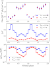 |
Fig. 6. Simulated CTA view of LS 5039 orbital variations above 1 TeV energy for 0.5 and 5 h long snapshots as observed from the southern CTA site. Upper panel: integral flux above 1 TeV, and middle and lower panels: estimated uncertainty of the measured spectral index and cut-off energy, correspondingly. The data points corresponding to Tobs = 5 h are shifted to the right by 0.01 phase for clarity. |
Figure 6 shows that the CTA can follow the orbital flux evolution of LS 5039 even with 30 min observational snapshots. However, in the orbital phase range 0.1 − 0.3, the uncertainties on the flux become ≳20% and at least 5 h long exposures would be required to determine the flux accurately. Such exposure times yield ≲10% accuracy of the flux and spectral index determination in this phase range, whereas the cut-off energy cannot be measured accurately. Only during the bright flux period, corresponding to the phase range ≈0.4 − 0.9, is the uncertainty in the cut-off energy better than ≈20%. This implies that detailed spectral studies of this particular binary phase will require integration over several orbital periods.
Such CTA observations of LS 5039 during its high-flux periods will enable spectral studies on timescales as short as 0.01 orbital periods (≈1 h). They will strongly constrain the physical processes at work.
Furthermore, it will clarify whether the rotating hollow-cone model (Neronov & Chernyakova 2008) that has previously been proposed to explain the LS 5039 TeV light curve is feasible. In this model, the TeV peak is composed of two narrower peaks, whose appearance depends on the location of the emission region and the system geometry. Neronov & Chernyakova (2008) suggested that the flux difference between the peaks and inferior conjunction at phase ≈0.7 is ≳10%. Such variations are detectable with CTA in several hours of exposure, as the top panel of Fig. 6 shows. In this way, CTA observations may allow constraining the geometry of the system, including the otherwise elusive orbital inclination angle.
3.4. 1FGL J1018.6−5856
3.4.1. Source properties
1FGL J1018.6−5856 (3FGL J1018.9−5856, HESS J1018−589A) is a point like γ-ray source. It is positionally coincident with the supernova remnant SNR G284.3–1.8. Using the Gaia DR2 source parallax and assuming a Gaussian probability distribution for the parallax measurement, Marcote et al. (2018) derived a source distance of  kpc. They also calculated the Galactic proper motion of the source and found that it is moving away from the Galactic plane. Both the source distance and proper motion are not compatible with the position of the SNR G284.3−1.8 (which is located at an estimated distance of ≃2.9 kpc). Therefore, it is possible to exclude any physical relation between the binary source and the SNR.
Spectroscopic observations of the optical counterpart allowed Strader et al. (2015) to find that a companion star has a low radial velocity semi-amplitude of 11–12 km s−1, which favours a NS as a compact object. This conclusion is in agreement with the results of Monageng et al. (2017), who constrained the eccentricity of the orbit e = 0.31 ± 0.16 and showed that the compact object is a NS, unless the system has a low inclination i ≲ 26°.
The 1FGL J1018.6–5856 was detected in a blind search for periodic sources in the Fermi-LAT survey of the Galactic Plane. Optical observations show that the non-thermal source is positionally coincident with a massive star of spectral type O6V(f). The radio and X-ray fluxes from the source are modulated with the same period of 16.544 days, interpreted as the binary orbital period (Fermi LAT Collaboration 2012).
The very high-energy counterpart of this source is the point-like source HESS J1018−589A, (H.E.S.S. Collaboration 2012a). In a dedicated observation campaign at VHE, HESS J1018−589A was detected up to 20 TeV. Its energy spectrum is well described with a power-law model, with a photon index Γ = 2.2 and a mean differential flux N0 = (2.9 ± 0.4)×10−13 ph cm−2 s−1 TeV−1 at 1 TeV. As in the case of other γ-ray binaries, the VHE spectrum cannot be extrapolated from the HE spectrum, which has a break at around 1 GeV. The orbital light curve at VHE peaks in phase with the X-ray and HE (1–10 GeV) light curves.
Based on optical spectroscopic observations, Strader et al. (2015) found that the maxima of the X-ray, HE, and VHE flux correspond to the inferior conjunction. This finding was unexpected because γ-rays are believed to be produced through anisotropic inverse Compton up-scattering of the stellar UV photons. Therefore, the peak of the γ-ray flux should occur at the superior conjunction, especially if the system is edge-on. This discrepancy could only be explained if the binary orbit is eccentric and the flux maximum occurs at periastron.
NuSTAR observations (An et al. 2015) demonstrated that similar to other γ-ray binaries, the broad-band X-ray spectrum is well fitted with an unbroken power-law model. The source flux shows a correlation with the spectral hardness throughout all orbital phases.
A comparison of the light curves of 1FGL J1018.6−5856 at different energy ranges shows that both the X-ray and the low-energy (E < 0.4 GeV) γ-ray bands are characterised by a similar modulation (a broad maximum at ϕ = 0.2–0.7 and a sharp spike at ϕ = 0), thus suggesting that they are due to a common spectral component. On the other hand, above ≈1 GeV, the orbital light curve changes significantly because the broad hump disappears and the remaining structure is similar to the light curve observed at VHE. Based on these results, An & Romani (2017) suggested that the flux in the GeV band is due mainly to the pulsar magnetosphere, while the X-ray flux is due to synchrotron emission from shock-accelerated electrons and the TeV light curve is dominated by the up-scattering of the stellar and synchrotron photons through external Compton (EC) and synchrotron self-Compton (SSC) mechanisms, in an intrabinary shock. The light curves at different energy ranges can be reproduced with the beamed SSC radiation from adiabatically accelerated plasma in the shocked pulsar wind. This is composed of a slow and a fast outflow. Both components contribute to the synchrotron emission observed from the X-ray to the low-energy γ-ray band, which has a sinusoidal modulation with a broad peak around the orbit periastron at ϕ = 0.4. On the other hand, only the Doppler-boosted component reaches energies above 1 GeV, which are characterised by the sharp maximum that occurs at the inferior conjunction at ϕ = 0. This result can be obtained with an orbital inclination of ≈50° and an orbital eccentricity of ≈0.35, consistent with the constraints obtained from optical observations. In this way, the model could also explain the variable X-ray spike coincident with the γ-ray maximum at ϕ = 0.
3.4.2. Prospects for CTA observations
Although 1FGL J1018.6−5856 was investigated in depth over the past few years, several question about its properties are still open, such as the physical processes that produce the HE/VHE emission. Moreover, it is still not clear whether the X-ray and γ-ray peaks are physically related to the conjunctions or the apastron and periastron passages. Therefore, the observation of this source with CTA will allow us to address a few topics. The high sensitivity of CTA will enable us to investigate the orbital modulation of the source spectrum and to study the correlation of the VHE emission with the system geometry. From the spectral point of view, the spectral shape will be further constrained at both the low (E < 0.1 TeV) and the high (E > 20 TeV) energy end. This will provide further constraints on the location, magnetic field, and acceleration efficiency of the VHE emitter (Khangulyan et al. 2008b) and on the opacity due to pair production (Böttcher & Dermer 2005; Dubus 2006).
To study the CTA capabilities, we first simulated the phase-averaged spectrum of the source based on the H.E.S.S. observations (H.E.S.S. Collaboration 2015a). As input we assumed a simple power-law emission with a photon index Γ = 2.2 and a flux normalisation N0 = 2.9 × 10⁻¹⁹ MeV−1 cm−2 s−1 at 1 TeV. We performed three sets of simulations for 30 min, 5 h, and 50 h observations. For each set we performed 100 simulations. Figure 1 shows that with a 5 h observation, it will be possible to measure the source flux and spectral slope with an uncertainty of ≃10% and 0.05, respectively. With only 30 min of observation, the corresponding errors would be ≃35% and 0.3.
In Fig. 7 we report the simulated spectrum of 1FGL J1018.6−5856 obtained with 50 h of observation, together with that obtained with 63 h of H.E.S.S. observations. It shows that the CTA spectrum is well determined both at low (down to E ≃ 0.1 TeV) and high energies (up to E ≃ 100 TeV), thus providing a significant enlargement of the spectral coverage compared to H.E.S.S.. The extension of the spectral range towards low energies will enable investigating the connection to the MeV–GeV emission, while the increase of the high-energy end will be important to constrain the cut-off linked to particle acceleration. We estimate that with a 5 h observation, the CTA will allow us to detect a high-energy cut-off if it is located below 18 TeV (Fig. 1).
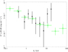 |
Fig. 7. Real and simulated spectra of 1FGL J1018.6−5856. Black: spectrum of 1FGL J1018.6−5856 obtained with 63 h of observation with H.E.S.S. (H.E.S.S. Collaboration 2015a). Green: simulation of the source spectrum obtained with 50 h of observation with CTA. |
We also studied the flux modulation of the source throughout the orbit. Following H.E.S.S. Collaboration (2015a), we divided the whole orbit into ten phase bins (1 bin ≃ 39.67 h) and assumed a simple photon spectrum with a power-law model with a slope Γ = 2.2. For each phase bin we performed 100 simulations for both 30min and 5h observations. We fitted the spectrum with a simple power-law model, keeping both the normalisation and the photon index Γ free to vary. The results of this set of simulations are reported in Fig. 8, where we show the variability (throughout the orbital phase) of the flux, its relative error, and the uncertainty of the index.
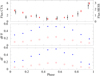 |
Fig. 8. Simulated CTA view of 1FGL J1018.6−5856 orbital variability. Upper panel: flux modulation of 1FGL J1018.6−5856 throughout the orbital phase as observed with H.E.S.S. (black symbols, in units of 10−12 ph cm−2 s−1 for E > 0.35 TeV) and simulated for 5 h of observation with the CTA (red symbols, in units of 10−13 ph cm−2 s−1 for E > 1 TeV). Middle panel: flux relative error in the case of simulated CTA observations of 30 min (blue filled squares) and 5 h (red open squares). Lower panel: uncertainty of the photon index Γ in the same cases. |
In the upper panel of Fig. 8, we report with red symbols the simulated light curve obtained with a campaign of 5 h observations for each phase bin with the CTA. It proves that in this case, the CTA can clearly resolve the source flux variability throughout the orbit. It will be possible to point out flux variations of ≃25% over timescales of ≈0.1 orbital periods (middle panel), and even at its flux minimum, the source will be detected with a significance ≳7σ. For comparison, in the upper panel of Fig. 8 we report as black symbols the folded light curve obtained with H.E.S.S. (with ≃8 h of observation for each phase bin). We note that in this case, it is possible to claim a clear flux variability only in the three phase bins in the phase range ϕ = 0.8–1.1, while the flux values measured in the remaining phase range are consistent with each other. The better characterisation of the source variability provided by the CTA will enable an improved correlation with the X-ray and HE variability and will place tighter constraints on the position and size of the VHE emitter.
The lower panel of Fig. 8 shows that even at the flux minimum, 5 h of observation with the CTA will provide a measurement of the photon index with an uncertainty of 0.2 (≃9%). This accuracy is comparable to that obtained with more than 60 h of observation with H.E.S.S. Therefore, it will be feasible to determine possible spectral variations > 10% in the orbital phase. In this way, it will be possible to single out the VHE emission and absorption processes and to obtain useful information on both the source magnetic field and the efficiency of the particle acceleration and pair production.
3.5. HESS J0632+057
3.5.1. Source properties
In contrast to other γ-ray loud binaries, HESS J0632+057 remained the only system that for a time was lacking detection in the GeV energy band. Only recently have indications of a GeV detection with Fermi-LAT been reported by Malyshev & Chernyakova (2016) and Li et al. (2017). The system was initially discovered during H.E.S.S. observations of the Monoceros region (Aharonian et al. 2007) as an unidentified point-like source. Its spatial coincidence with the Be star MWC 148 suggested its binary nature (Aharonian et al. 2007; Hinton et al. 2009). With dedicated observational campaigns, the binary nature of the system was confirmed by radio (Skilton et al. 2009) and soft X-ray (Falcone et al. 2010) observations. In the TeV band, the system was also detected by VERITAS and MAGIC (Aleksić et al. 2012c; Aliu et al. 2014).
The orbital period of HESS J0632+057 of ≈316 ± 2 d (Malyshev et al. 2017), with a zero-phase time T0 = 54857 MJD (Bongiorno et al. 2011), was derived from Swift/XRT observations. The exact orbital solution and even the orbital phase of periastron is not firmly established and is placed at orbital phases ϕ ≈ 0.97 (Casares et al. 2012) or ϕ ≈ 0.4 − 0.5 (Moritani et al. 2018; Malyshev et al. 2017).
The orbital folded X-ray light curve of HESS J0632+057 has two clear emission peaks: first at phase ϕ ≈ 0.2 − 0.4, and second at ϕ ≈ 0.6 − 0.8 separated by a deep minimum at ϕ ≈ 0.4 − 0.5 (Bongiorno et al. 2011; Aliu et al. 2014). A low-intermediate state is present at ϕ ≈ 0.8 − 0.2. The orbital light curve in the TeV energy range shows a similar structure, as was reported by Maier & VERITAS Collaboration (2015). Indications of orbital variability in the GeV range were reported by Li et al. (2017).
The X-ray-to-TeV spectrum of HESS J0632+057 is shown in Fig. 9. Several models have been proposed so far to explain the observed variations of the flux and spectrum throughout the orbit. In the flip-flop scenario (see e.g. Moritani et al. 2015, and references therein) the compact object is assumed to be a pulsar that passes periastron at ϕ = 0.97. Close to apastron (orbital phases ≈0.4P − 0.6), the pulsar is in a rotationally powered regime, while it switches into a propeller regime when periastron is approached (phases 0.1 − 0.4 and 0.6 − 0.85). When the gas pressure of the Be disc overcomes the pulsar-wind ram pressure, the pulsar wind in a flip-flop scenario is quenched (phases 0 − 0.1 and 0.85 − 1). Because the Be disc of the system is estimated to be about three times larger than the binary separation at periastron, the compact object enters a dense region of the disc near periastron. In this situation, the strong gas pressure is likely to quench the pulsar wind and suppress high-energy emissions. Alternatively, the observed orbital variations can be explained within the “similar to PSR B1259−63” model (Malyshev et al. 2017). The similar two-peak behaviour of the HESS J0632+057 and PSR B1259−63 orbital light curves allows us to assume that the orbital plane of HESS J0632+057 is inclined with respect to the disc plane, similarly to PSR B1259−63. Orbital X-ray and TeV peaks within this model correspond to the first and second crossing of the disc by a compact object. Higher ambient density during these episodes leads to more effective cooling of the relativistic electrons by synchrotron and inverse Compton mechanisms, resulting in an increased level of X-ray and TeV emission. The orbital phase of periastron in this model is located at phase ϕ ≈ 0.4 − 0.5 (Malyshev et al. 2017).
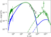 |
Fig. 9. X-ray-to-TeV spectrum of HESS J0632+057 during its high state (green points; orbital phases ϕ ≈ 0.3 − 0.4) and low state (blue points; ϕ ≈ 0.4 − 0.5). The data are adopted from Malyshev et al. (2017) (X-rays), Li et al. (2017) (mean GeV spectrum, black points), and Malyshev & Chernyakova (2016) (green upper limits). TeV data are adopted from Maier & VERITAS Collaboration (2015). The solid lines show the “similar to PSR B1259−63” model flux, while dashed and dot-dashed lines illustrate contributions from synchrotron and IC model components correspondingly. See text for more details. |
The break in the GeV–TeV spectrum at ≈200 GeV can be interpreted as a corresponding break in the spectrum of emitting relativistic electrons. The X-ray-to-GeV and TeV parts of the spectrum are explained as synchrotron and IC components. An initial power-law (Γ1, e ≈ 1.3) spectrum of electrons can be modified by synchrotron energy losses at above Ebr ≈ 1 TeV, resulting in a Γ2, e ≈ 2.3 higher energy slope. The absence of cooling in the energy band below 1 TeV could be attributed to the escape of the sub-TeV electrons from the system. A similar interpretation of the spectral energy distribution was proposed by Chernyakova et al. (2015) for PSR B1259−63.
Alternatively, the spectral break in the electron spectrum can occur at the transition between the domination of adiabatic and IC or synchrotron losses (see e.g. Khangulyan et al. 2007 and Takahashi et al. 2009 for PSR B1259−63 and LS 5039). The adiabatic loss time is naturally shortest in sparse regions outside of the Be star disc and longest in dense regions inside it.
A broken power-law shape of the spectrum is not unique for the “similar to PSR B1259−63” model. A similar shape of the spectrum can also be expected within the flip-flop model because both interpretations of the break origin can be valid for this model. The two models can be distinguished by CTA observations of the variation in slope and low-energy break position throughout the orbit.
Within the flip-flop model at orbital phases ϕ = 0 − 0.4, the compact object moves from a denser to increasingly sparser regions of the Be star disc. The spectrum of relativistic electrons becomes increasingly less dominated by the losses. This results in a gradual hardening of the TeV slope and in a shift of the break energy to higher values. At phases ϕ ≈ 0.6 − 1, the compact object enters denser regions of the disc, which should lead to a gradual softening of the slope and shift of the energy break to lower energies. The spectrum is expected to be hardest when the object is beyond the Be star disc (orbital phase ≈0.4). This phase corresponds to the minima of observed emission. The softest spectrum is expected when the compact object approaches periastron, that is, at phase ϕ ≈ 0.97.
In the “similar to PSR B1259−63” model the compact object intersects the disc of the Be star twice per orbit (at orbital phases 0.2 − 0.4 and 0.6 − 0.8) where the soft spectrum with the low position of energy break is expected. At phases 0 − 0.2, 0.4 − 0.6 and 0.8 − 1 in the “similar to PSR B1259−63” model, the compact object is beyond the dense regions of the disc. At these orbital phases a hard slope with energy break shifted to higher energies can be expected.
3.5.2. Prospects for CTA observations
Because of its location, HESS J0632+057 is visible from both the north and south CTA sites (see Table 1). For our simulations we considered two orbital phases: the brightest phase (ϕ = 0.2–0.4, hereafter the “high state”) based on Aliu et al. (2014), and the low-intermediate phase (ϕ = 0.8–0.2, hereafter the “low state”) based on Schlenstedt (2017). No spectra are reported in the literature for the deep minimum state at ϕ = 0.4–0.5 and the two maxima have similar spectra, therefore we chose the brightest as representative of the active state.
In the first group of simulations, we considered the 0.1–100 TeV energy range. The spectral model component of the source was defined as a power-law model with either a photon index 2.3 and normalisation at 1 TeV of 5.7 × 10⁻¹³ ph cm−2 s−1 TeV−1 (ϕ = 0.2–0.4, high state), or a photon index 2.72 and normalisation 2.3 × 10⁻¹³ ph cm−2 s−1 TeV−1 (ϕ = 0.8–0.2, low state).
The dependence of the source flux and index uncertainties on different configurations is shown in Fig. 1 for 30 min and 5 h observations. Simulations also show that a longer 50 h observation can reconstruct the flux and slope of the source to an accuracy of better than 3% in the Northern and Southern Hemispheres.
In the second group of simulations, we simulated the source spectrum with a broken power-law model to study the possibility of the detection of a low-energy break. The two physical scenarios discussed above, flip-flop versus “similar to PSR B1259−63”, can be distinguished by CTA observations of the variation in the position of the slope and low-energy break throughout the orbit. In both high and low states, we used a low-energy slope fixed at 1.6 and an energy break at 0.4 TeV (the value of the break energy was not fixed in the simulations, therefore it can vary between different realisations, Malyshev & Chernyakova 2016). The high-energy slopes are given by the spectral indices already discussed: Γ = 2.3 for the ϕ = 0.2–0.4 high state, and Γ = 2.72 for the ϕ = 0.8–0.2 low state. The normalisations for the two states at 0.4 TeV are 4.7 × 10⁻¹² ph cm−2 s−1 TeV−1 (high state), and 2.8 × 10⁻¹² ph cm−2 s−1 TeV−1 (low state). For these simulations, we focused on the southern site and the 0.04–100 TeV energy range. Simulations of 5 h and 50 h observations were performed, and the results are shown in Table 2.
Figure 10 shows two single realizations of the spectra of HESS J0632+057, 5 h (left) versus 50 h (right). Upper limits are shown when the detection significance is lower than 3σ. A 50 h observation will excellently reconstruct the energy break and slopes, whereas a 5 h observation will suffer from higher uncertainties.
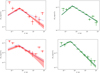 |
Fig. 10. Simulated spectra (red and green points) of HESS J0632+057, as observed from the southern site. In blue we show the input models. Upper left: high state, 5 h. Upper right: high state, 50 h. Lower left: low state, 5 h. Lower right: low state, 50 h. |
A direct comparison of the same power-law spectra simulated for the CTA with respect to H.E.S.S. (Aliu et al. 2014) and VERITAS (Schlenstedt 2017) observations shows that a CTA snapshot of 5 h will result in more accurate results than what was previously obtained. A 55 h observation of the low state (ϕ = 0.8–0.2) of the source with VERITAS resulted in a ≈7% uncertainty on the detected slope (2.72 ± 0.2), to be compared to the ≈5% with a 5 h CTA south observation. Similarly, a 15 h observation of the high state with H.E.S.S. resulted in a ≈9% uncertainty on the detected slope (2.3 ± 0.2), to be compared to the ≈3% with a 5 h CTA south observation. The CTA error estimates given here are purely statistic, whereas the VERITAS and H.E.S.S. results include systematic errors as well.
Figure 1 and Table 2 show that a 5 h observation will be enough to distinguish the low state from the high state, but it may not be enough to unambiguously distinguish the energy break (≈30% uncertainty). A 50 h observation would result in a 10% uncertainty of the energy break (15% for a 20 h observation), allowing the high-energy slope and energy break to be accurately monitored throughout the orbit. This would enable the CTA to distinguish the two currently available scenarios, that is, flip-flop versus “similar to PSR B1259−63”, which expect an opposite trend of the spectral slope and energy break from the high state to the low state: a hardening of the spectrum and Eb moving to higher energies for the “similar to PSR B1259−63” scenario versus a softening of the spectrum and Eb moving to lower energies in the flip-flop model.
HESS J0632+057 has a long orbital period (≈316 d), and each phase will occur only once in one year of observations. Nevertheless, each state is observable for a long period, therefore a 50 h observation in the same state (10 nights with ≈5 h each) is possible.
3.6. HESS J1832−093
3.6.1. Source properties
HESS J1832−093 is a new γ-ray binary candidate discovered as a TeV point source by H.E.S.S. This source lies in the vicinity of SNR G22.7−0.2, which might suggest an association with this SNR (H.E.S.S. Collaboration 2015b). However, several follow-up observations in X-rays instead support the binary nature of this source (Eger et al. 2016; Mori et al. 2017). A simple power-law model describes the TeV spectrum well, with a photon index of Γ = 2.6 ± 0.3stat ± 0.1sys and an integrated photon flux above 1 TeV of F = (3.0 ± 0.8stat ± 0.6syst)×10−13 cm−2 s−1 (H.E.S.S. Collaboration 2015b). An XMM-Newton observation of the source field discovered a bright X-ray source, XMMU J183245−0921539, within the γ-ray error circle (H.E.S.S. Collaboration 2015b). This source is also associated with a point source detected in a subsequent Chandra observation campaign (Eger et al. 2016). During the Chandra observations, an increase of the 2–10 keV flux of the order of 4 with respect to the earlier XMM-Newton measurement and the coincidence of a bright IR source at the Chandra error box suggest a binary scenario for the γ-ray emission (Eger et al. 2016).
Recently, Mori et al. (2017) reported on a NuSTAR X-ray observation of the field containing HESS J1832−093 and a re-analysis of the archival Chandra and XMM-Newton data. The data reanalysis does not confirm the same level of flux variation as was reported in previous work. However, Mori et al. (2017) found other evidence that supports the γ-ray binary scenario for this source: the X-ray NuSTAR spectrum extends to 30 keV, and the best fit is represented by a simple power-law model with a photon index of Γ = 1.5 without any break or cut-off. The NuSTAR 2–10 keV flux is 1.5 times higher than the 2011 XMM-Newton flux in the same range. Even if no pulsations were detected in the power spectrum, the flat power density spectrum underlines the lack of accretion-powered emission from the source. The authors conclude that the X-ray timing properties of HESS J1832−093 are similar to those of the other γ-ray binaries. Currently, no GeV emission has been detected from the system, however (Eger et al. 2016; H.E.S.S. Collaboration 2015b). A reliable identification of HESS J1832−093 as a γ-ray binary still needs the detection of the orbital period as well as simultaneous X-ray and γ-ray observations.
During the H.E.S.S. measurement no significant flux variability was detected in the long term light curves (run, day, month, as reported by H.E.S.S. Collaboration 2015a). The data set consisted of 67 h of observations taken from 2004 to 2011. Even if the data sample has a low density, the lack of flux variability could imply that the eventual modulation of the γ-ray flux is probably quite smooth and mostly within the H.E.S.S. flux error (the H.E.S.S. statistical error is about 26%). Even if the X and γ-ray characteristics resemble those of HESS J0632+057, the orbital period is probably long, similar to that of PSR B1259−63, for instance.
3.6.2. Prospects for CTA observations
We performed two sets of a 1000 simulations for 0.5 h and 5 h exposure time, respectively. The input source spectrum had a power-law shape with a slope Γ = 2.6, as reported by H.E.S.S. Collaboration (2015a). The simulation results are shown in Fig. 1. The results of our simulations show that the source is too faint to be firmly detected in 30 min, but for 5 h, we obtained a ≈14σ detection. Moreover, CTA observations of HESS J1832−093 will surely improve the angular resolution, allowing further constraints on the extension of the TeV source. The spectrum measurements will be extended both below and above the H.E.S.S. detection, which will allow eventual detection of a spectral cut-off. Simulations reported in Fig. 1 demonstrate that with a 5 h exposure, the CTA will be able to detect a high-energy cut-off if it is present below 10 TeV. Finally, the high CTA sensitivity could detect flux variation and spectral modulation. In particular, a detection of flux modulation will allow us to fix the orbital period, which is the first step for a reliable identification of HESS J1832−093 with a γ-ray binary.
3.7. LMC P3
3.7.1. Source properties
LMC P3 is the first and currently only known extragalactic γ-ray binary. It was detected in 2016 with the Fermi-LAT in the Large Magellanic Cloud in a search for periodic modulation in all sources in the third Fermi-LAT catalogue (Acero et al. 2015). The system has an orbital period of 10.3 days and is associated with a massive O5III star located in the supernova remnant DEM L241 (Corbet et al. 2016). Swift/XRT X-ray and ATCA radio observations demonstrated that both X-ray and radio emission are also modulated on the 10.3 day period, but are in anti-phase with the γ-ray modulation. The X-ray spectrum is well described by a single power law with Γ = 1.3 ± 0.3, modified by a fully covered absorber. The resulting value of the hydrogen column density of a fully covered absorber is comparable with the Galactic HI value.
Optical radial velocity measurements suggest that unless the system has a very low inclination, the system contains a NS (Corbet et al. 2016). Low inclinations, however, result in a range of masses of the compact object above the Chandrasekhar limit, for example, a BH with a mass of M = 5 M⊙ will have an inclination  , and i = 8 ± 2° for M = 10 M⊙. The source is significantly more luminous than similar sources in the Milky Way at radio, optical, X-ray, and γ-ray wavelengths. It is at least four times more luminous in GeV γ-rays and ten times more luminous in radio and X-rays than LS 5039 and 1FGL J1018.6−5856, although the luminosity of the companion star and the orbital separations are comparable in all three systems.
The LMC has been extensively observed with H.E.S.S. since 2004. The data that were collected for the LMC between 2004 and the beginning of 2016 result in an effective exposure time for LMC P3 of 100 h (H.E.S.S. Collaboration 2018). The sensitivity of H.E.S.S. does not allow a detection of flux variations of the object on a nightly basis. The low flux coming from the system does not allow for any statistically significant detection of periodicity using a Lomb-Scargle test and the Z-transformed discrete correlation function. Folding the light curve with the orbital period of the system of 10.301 days clearly demonstrates the orbital modulation of the VHE with a significant detection only in the orbital phase bin between 0.2 and 0.4 (orbital phase-zero is defined as the maximum of the HE light curve at MJD 57410.25). The H.E.S.S. spectrum during the on-peak part of the orbit is described by a power law with a photon index Γ = 2.1 ± 0.2. The averaged slope throughout the total orbit is softer with Γ = 2.5 ± 0.2. The VHE flux above 1 TeV varies by a factor more than 5 between on-peak and off-peak parts of the orbit.
The minimum HE emission occurs between orbital phases 0.3–0.7. The shift between the orbital phase of HE and VHE peaks is not unique to this γ-ray binary. For example, a similar shift is observed in LS 5039 (see Sect. 3.3), as the angle-dependent cross section of IC scattering and γγ absorption due to pair-production affects the HE and VHE in different ways (e.g. Dubus et al. 2008; Khangulyan et al. 2008b; Neronov & Chernyakova 2008).
Recently reported optical spectroscopic observations of LMC P3 have better constrained the orbital parameters (van Soelen et al. 2019). The observations find that the binary has an eccentricity of 0.4 ± 0.07. They place superior conjunction at phase ≈0.98 and inferior conjunction at phase ≈0.24. These phases correspond to the points of the maxima reported in Fermi-LAT and H.E.S.S. light curves, respectively. The mass function (≈0.0010 M⊙) favours a NS companion for most inclination angles. The detection of VHE emission during the entire orbit is critical for detailed modelling that will allow us to understand what is happening in the system.
3.7.2. Prospects for CTA observations
Following the results of H.E.S.S. observations, we simulated light curves and spectra that the CTA will observe during the high (FTeV = 5 × 10⁻¹³ cm−2 s−1) and low (FTeV = 1 × 10⁻¹³ cm−2 s−1) states, where FTeV is the source flux above 1TeV. In our simulations, we assumed a constant flux within each of the states. The results are presented in Fig. 11. During the high state, the CTA will be able to detect variability of the source at a 3σ confidence level if it is higher than 60% on a 30 min time scale, and 40% on a one-hour timescale.
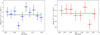 |
Fig. 11. Simulated CTA light curves of LMC P3 at high (left panel, 30 min time bin) and low (right panel, 5 h time bin) states. |
In Fig. 12 we show the spectra of the high and low states of the source. We will be able to determine the slope of the spectrum with an accuracy of 2% for 5 h of observations (6% for one hour) during the high state, and 2% for 40 h observations (10% for 5 h) during the low state.
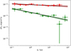 |
Fig. 12. Simulated CTA spectrum of LMC P3 at high (red points, 5 h exposure) and low (green points, 40-h exposure) states. |
Thus the CTA sensitivity will be high enough to study the nightly averaged spectral evolution of the source with an accuracy of better than 10% throughout the orbit. This will allow us to understand the details of the physical processes in this system and develop a consistent model of the multi-wavelength emission.
4. Colliding-wind binaries
4.1. η Carinae
4.1.1. Source properties
η Carinae is the most luminous massive binary system in our Galaxy, and the first binary that does not host a compact object that has been detected at VHEs. It is believed to be composed of a luminous blue variable, possibly originating as a star with an initial mass ≳90 M⊙ (Hillier et al. 2001), and of a Wolf–Rayet (WR) companion. The former is accelerating a very dense wind with a mass-loss rate of ≈8.5 × 10⁻⁴ M⊙ yr−1 and a terminal velocity of ≈420 km s−1 (Groh et al. 2012). Based on the observed X-ray emission of this system, it is believed that its companion also emits a powerful wind, with mass-loss rates of ≃10−5 M⊙ yr−1 at a velocity of 3000 km s−1 (Pittard & Corcoran 2002; Verner et al. 2005; Falceta-Gonçalves et al. 2005; Parkin et al. 2009, see Table 3).
System parameters of CWBs.
The inference of binarity for η Car is indirect because the companion is not directly observed at any wavelength. Spectral periodic variations have been used to indicate its binary nature and to provide estimates of both the orbital and the companion stellar parameters. The modulation detected in the X-ray light curve indicates that the two stars are on a highly eccentric orbit (Corcoran et al. 2001; Falceta-Gonçalves et al. 2005; Okazaki et al. 2008), while its hardness and intensity allow for the estimates of the wind velocity and mass-loss rate shown in Table 3.
During its great eruption (1837–1856), η Car ejected 10 − 40 M⊙ (Gomez et al. 2010) at an average speed of ≈650 km s−1 (Smith et al. 2003), forming the Homunculus nebula and releasing 1049 − 50 erg of energy. The orbital period at the epoch of the great eruption was ≈5.1 yr, and increased to the current ≈5.54 yr (Whitelock et al. 2004; Corcoran 2005; Damineli et al. 2008). Two other major eruptions occurred since then (Abraham et al. 2014), resulting in ejecta that interact with the radiation coming from within. The long-term X-ray modulation observed for different orbits is possibly due to the time evolution of the ejecta.
The relative separation of the two stars varies by a factor ≈10 − 20, depending on the estimated eccentricity (e ≈ 0.9 − 0.95). At periastron, the two objects pass within a few AU of each other, a distance just a few times larger than the size of the primary star. In these extreme conditions their supersonic winds form a colliding-wind region of hot shocked gas where charged particles can be accelerated through diffusive-shock acceleration up to HEs (Eichler & Usov 1993; Dougherty et al. 2003; Reimer et al. 2006). As these particles encounter conditions that vary throughout the orbit, we can expect an orbital dependency of the γ-ray emission.
The hard X-ray emission detected by INTEGRAL (Leyder et al. 2008) and Suzaku (Okazaki et al. 2008), with an average luminosity (4–7)×1033 erg s−1, suggested the presence of relativistic particles in the system. AGILE detected a variable γ-ray source compatible with the position of η Car (Tavani et al. 2009b). Fermi-LAT detected very energetic emission ≳10 GeV around periastron (Abdo et al. 2010; Farnier et al. 2011; Reitberger et al. 2012) that can be interpreted as the π0-decay of accelerated hadrons interacting with the dense stellar wind (Farnier et al. 2011). Other authors assumed that the intrinsic cut-off of the γ-ray spectrum can be placed at higher energies (250 − 500 GeV), whilst the observed final spectrum is the consequence of the γ-γ absorption over an ad hoc distribution of soft X-ray photons (Reitberger et al. 2012).
Cherenkov observations (H.E.S.S. Collaboration 2012b; Leser 2017) imply a sudden drop in the spectrum at energies ≳1 TeV that could be interpreted as a cut-off in the accelerated particle distribution or due to severe γ-γ absorption.
4.1.2. γ-ray variability
Parkin et al. (2011) presented three-dimensional hydrodynamical simulations of η Car that reproduced the observed X-ray spectra and light curves. The acceleration of particles to relativistic energies also depends on the magnetic field of the shock region. The first magnetohydrodynamical (MHD) simulations of the colliding winds in η Car was performed by Falceta-Gonçalves & Abraham (2012). The authors showed that the amplification factor of the field within the shocks is orders of magnitude larger than the estimates from Rankine–Hugoniot jump conditions because of the pile-up effect (Rocha da Silva et al. 2015).
With respect to the energetic particles, Falceta-Goncalves (2015) numerically integrated particle trajectories on top of the previous MHD simulations in order to study their acceleration. The author showed that the complex geometry of the field at the cooled shock region results in diffuse acceleration to be more efficient than the first-order Fermi process. Maximum energies of 1 − 10 TeV where obtained for the typical wind parameters of the system. Unfortunately, the number of particles simulated was insufficient to fully predict the probability distribution function of the energetic particles and the consequent spectral energy distribution of the radiation. To estimate the non-thermal emission of the system, Balbo & Walter (2017) calculated the maximum energies reached by electrons and hadrons cell by cell, assuming a dipolar magnetic field at the surface of the main star. The magnetic field is the only additional parameter and can be tuned. Shock velocities and mechanical power were calculated in every cell, including those outside the shock region. Most of the shock power is released on both sides of the wind collision zone and in the cells downstream of the wind-collision region (Reimer et al. 2006). The increasing shock area compensates for the loss of the released energy density up to a relatively large distance from the centre of mass, explaining why the X-ray luminosity at apastron is still about one-third of the peak emission at periastron.
The optical depth of the wind for γ-ray absorption varies between 10−6 at apastron and ≈10−2 at periastron. This means that the 1–100 GeV spectral shape cannot be explained by absorption (Reitberger et al. 2012).
The mechanical luminosity available in the shock increases towards periastron (the same trend is followed by the thermal emission) and almost doubles in the phase range ≈1.05 − 1.15. The latter peak corresponds to a bubble with reverse-wind conditions developing and effectively doubling the shock-front area during about a tenth of the orbit (Parkin et al. 2011). The density of this bubble is low, its thermal emission does not contribute significantly. The mechanical luminosity shows a local minimum between phases 1.0 and 1.05, when the central part of the wind collision zone is disrupted. Phases 1 and 2 correspond to first (2009) and second (2014) periastron observed during Fermi-LAT operation epoch, respectively.
Electron cooling through inverse-Compton scattering is very efficient and the induced γ-ray flux peaks just before periastron. Because of the bubble mentioned above, a secondary inverse-Compton peak is expected above phase 1.05, although its spectral shape could be different. The relative importance of the secondary peak depends on the magnetic field geometry, radiation transfer, obscuration, and details of the hydrodynamics. The situation is different for hadrons. Unless the magnetic field is very strong (> kG), hadronic interactions mostly take place close to the centre and a single peak of π0 decay is expected before periastron.
Figure 13 shows the X-ray and γ-ray light curves predicted by the simulations for a surface magnetic field of 500 G and assuming that 1.5% and 2.4% of the mechanical energy is used to accelerate electrons and protons, respectively. To facilitate the comparison between observations and simulations, the results of the latter were binned in the same way as the observed data.
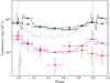 |
Fig. 13. Simulated and observed X-ray and γ-ray light curves of η Car. The black and purple lines and bins show the predicted inverse-Compton and π0-decay light-curves. The green and red points show the observed Fermi-LAT light curves at low (0.3–10 GeV) and high (10–300 GeV) energies. The dim grey light curves show the observed (continuous) and predicted (dash, without obscuration) thermal X-ray light curves. Error bars are 1σ. Phases 1 and 2 correspond to first (2009) and second (2014) periastron observed during Fermi-LAT operation epoch, respectively (from Balbo & Walter 2017). |
Such a surface magnetic field provides a good match to the observations, but magnetic field amplification at the shock could scale it down. The predicted flux at phase 1.1 is too high by a factor 2 when compared with the observation. This discrepancy largely comes from the energy released in the inverted-wind bubble after periastron. The ratio of the emission generated in the shocks on both sides of the wind collision zone is relatively constant throughout the orbit, except at phase 1.1, where much more power is generated in the shock that occurs in the wind of the secondary star. This discrepancy may indicate that the inverted bubble is either unstable or produces a significantly different inverse-Compton spectrum.
Observations match the predictions of the simulation except for the second peak, which is slightly shifted towards earlier phases and has a lower luminosity (see Fig. 6 in Balbo & Walter 2017). The phase difference could be related to the eccentricity (e = 0.9) that we assumed in the simulation, which is not well constrained by observations (Damineli et al. 2000; Corcoran et al. 2001), and that has an important effect on the inner shock geometry.
The distribution of the maximum electron energy, weighted by the inverse Compton emissivity, and hence the resulting photon distribution, are quite smooth. The difference in the electron spectral shape on both sides of the wind collision zone cannot account for the two γ-ray components, as suggested by Bednarek & Pabich (2011), who assumed a simplified geometry.
The inverse-Compton emission peaks slightly below 1 GeV and does not extend beyond 10 GeV at the level observed during first periastron (see Fig. 4 in Walter & Balbo 2018). This contradicts the conclusions from Ohm et al. (2015), who attributed the full Fermi-LAT detection to hadronic emission. Their simulations predict a smaller variation between periastron and apastron, a longer flare around periastron and a deeper minimum than in the observed data. These discrepancies might be due to the simplified geometry assumed by the authors and by the artificially reduced particle acceleration at periastron. Inverse-Compton emission and π0 decay (Farnier et al. 2011) therefore remain a good model of the γ-ray variability.
The simulated π0-induced γ-ray light-curve and its variability amplitude show a single peak of emission centred at periastron, in good agreement with the Fermi-LAT observations of first periastron. These simulations predict that the hadronic cut-off energy varies between 200 TeV and 2 TeV from periastron to apastron. η Car may therefore accelerate particles close to the knee of the cosmic-ray spectrum.
The second periastron is different, with a lack of high-energy emission. It has been suggested that the change in the X-ray emission after that periastron (a significant decrease can be observed in Fig. 13, see also Corcoran et al. 2015) was the signature of a change in wind geometry, possibly because of cooling instabilities. A stronger disruption or clumpier wind after second periastron might induce a decrease in average wind density and explain why fewer hadronic interactions and less thermal emission took place, without greatly affecting the inverse-Compton emission.
4.1.3. Prospects for CTA observations
The CTA telescopes to be placed in the Southern Hemisphere will be very sensitive and probe the spectrum and variability of η Car above 30 GeV. As discussed above, the contribution of the IC emission is negligible above 10 GeV and the observed VHE emission is only due to π0 decay. The π0 decay spectrum should be heavily modified by γ-γ absorption of TeV photons against the numerous ultraviolet photons emitted by the stellar surfaces. The photon field is probably opaque at 1 TeV, with an optical depth varying quickly depending on the relative position of the two stars and of the line of sight. The intrinsic π0 decay spectrum is a complex convolution of the maximum energy, luminosity, particle drift, and obscuration. The obscuration is likely maximised at periastron, when the ultraviolet photon field is particularly dense and the intrinsic cut-off energy is highest.
In the case of an isotropic radiation field, the optical depth could reach ≈10 at periastron. As the soft photon distribution is highly anisotropic, the absorption cross section will decrease and peak up to ϵ1ϵ2 > 10 MeV2 for γ-ray photons that leave the stars towards the observer (Voisin et al. 2018). This is consistent with the H.E.S.S. observations (Leser 2017) showing a cut-off at an energy higher than expected for an isotropic distribution of ultraviolet photons. The γ-ray spectrum cut-off energy and optical depth are expected to vary throughout the orbit (and viewing angle), showing a variability pattern that is indicative of the geometry and magnetic field configuration.
The CTA will follow these variations with a sensitivity that is orders of magnitude better than the sensitivity of Fermi-LAT, and will provide unique additional constraints on the model parameters. Provided that the loosely constrained optical depth is in a reasonable range, the π0 decay continuum could be detected up to 100 TeV with the small CTA telescopes. Figure 14 shows that the CTA could independently detect the cut-off of the π0 decay and the strength of the γ-γ absorption at apastron and periastron (see Walter & Balbo 2018). The CTA could follow the variability of these parameters throughout the orbit with a resolution of a few days to establish the nature of the high-energy component and constrain the geometry of the shock at the core of the system.
 |
Fig. 14. Shock-induced spectral energy distribution in η Car from 1 keV to 1 PeV. The data (black) are from NuSTAR (Panagiotou & Walter 2018), Swift/BAT, INTEGRAL, and Fermi-LAT. The red points are the H.E.S.S. measurements obtained close to periastron. Green points show a 50-hour simulated observation by the CTA at periastron. The blue line shows the spectrum that might be expected at apastron with a lower energy cut-off and obscuration. The system geometry can be constrained by a shift of the obscuration peak throughout the orbit, which is not taken into account here. The yellow dotted line is the 50 h CTA point-source sensitivity (5σ per bin of ΔE/E = 0.2). |
4.2. Prospective CWBs
To date, η Car is the only CWB that has been detected as a high and a very high-energy γ-ray source. Based on the results of theoretical modelling, Werner et al. (2013) highlighted a sample of seven other CWBs with WR-companions, WR 11, WR 70, WR 125, WR 137, WR 140, WR 146, and WR 147, as the most favourable candidate high-energy CWB sources. A Fermi-LAT analysis of these CWBs, using almost seven years of data, has been presented by Pshirkov (2016). As a result, three sources (WR 11, WR 125, and WR 147) have been detected with a significance that exceeds a test statistic of TS = 25, but only WR11 (part of the γ2 Vel binary system) does not suffer from background contamination. WR 11 (γ2 Vel) is also the only WR star with a counterpart in the FL8Y Source List (FL8Y J0809.4−4714, 6.8σ detection in the 100 MeV−1 TeV band). It lies within the 3σ error ellipse.
None of the other WR stars, including WR 125 and WR 147, has FL8Y counterparts. Of the proposed list of seven candidate sources, we only investigated γ2 Vel (which consists of WR 11 and an O7.5 star; see Table 3) as a prospective TeV CWB.
We also considered one other CWB candidate, the binary system HD 93129A, which consists of two O-type stars (see Table 3). We have found that the position of HD 93129A is well inside the 2σ error ellipse of an FL8Y source, FL8Y J1043.6−5930 (5σ detection), which is a counterpart to 3FGL J1043.6−5930.
4.2.1. γ2 Velorum
The system γ2 Vel is one of the most promising CWB candidates for detection at HE and VHE γ-rays. In addition to the powerful winds emittedf by both components (a WR and an O-type star) and the small binary separation (see Table 3), its main advantage is its close proximity: at only 340 pc, WR11 is the closest WR star to Earth. This binary has therefore been studied very well at different energy bands (see e.g. references in the Catalogue of Particle-Accelerating CWBs, De Becker et al. 2017).
Because the point spread function (PSF) of a Fermi-LAT source is ≈1°, the analysis of radio data with a high spatial resolution is very important for confirming the high-energy γ-ray association because radio observations can spatially separate additional sources such as nearby AGNs. Signatures of strongly attenuated non-thermal radio emission from this CWB have been revealed (Chapman et al. 1999), confirming (with caution) the status of γ2 Vel as a particle-accelerating CWB. In the region of Fermi-LAT enhancement lies is another potential high-energy γ-ray source, however: the extended (45″) radio source MOST 0808−471 with a non-thermal radio spectrum and parameters typical of a Faranoff–Riley (FR) FRI or FRII radio galaxy (Chapman et al. 1999). The absence of variability in the GeV emission prevents a firm conclusion on the nature of the observed GeV emission. X-ray (ASCA) and γ-ray (INTEGRAL) observations place only upper limits on a possible non-thermal component from γ2 Vel (Tatischeff et al. 2004).
The HE γ-ray spectrum of γ2 Vel, using seven years of Fermi-LAT data (in the 0.1–100 GeV energy range) was analysed in Pshirkov (2016). It was shown that fits with a power-law model (Γ = 2.16 ± 0.2; TS = 37.3), a log-parabola model (TS = 41.5), and a broken power-law model (TS = 44.3) do not represent the observed hardening of the spectrum at energies E > 10 GeV well (this hardening is similar to the spectrum of η Car during periastron). At a distance of d = 340 pc, the high-energy flux of F(0.1–100 GeV) = (2.7 ± 0.5) × 10−12 erg cm−2 s−1 corresponds to a luminosity of L = (3.7 ± 0.7) × 1031 erg s−1. This is only a small fraction (≈10−4) of the kinetic wind power that is dissipated in the colliding-wind zone (Pshirkov 2016; Reitberger et al. 2017).
The first three-dimensional MHD simulations of the colliding-wind region in γ2 Vel, which took into account the generation of γ-ray emission through diffusive-shock acceleration of protons and nuclei, and subsequent π0 decay has been presented by Reitberger et al. (2017). The Fermi-LAT data (Pshirkov 2016) can only be reproduced using a high WR mass-loss rate (ṀWR = 3 × 10⁻⁵ M⊙ yr−1), but the observed hardening of the γ-ray spectrum at 10–100 GeV is not reproduced because the simulated spectrum has a cut-off at 100 GeV because the accelerated protons reach a maximum energy of ≈1 TeV.
4.2.2. Prospects for CTA observations
To estimate the capability of the CTA of detecting γ2 Vel at TeV energies, we extrapolated the Fermi-LAT spectrum to the 0.1–10 TeV range. In our analysis we assumed F(E = 1 TeV) = 1.77 × 10⁻²⁰ ph cm−2 s−1 MeV−1 and a photon index Γ = 2.51. A simulated spectrum of a 50 h observation is shown in Fig. 15 (left panel). Even if the Fermi-LAT power-law spectrum really does extend up to 10 TeV, the source can only be detected with a low significance (10 < TS < 25) in the range 1–10 TeV (where the CTA sensitivity is highest) becaus of the low flux level.
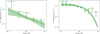 |
Fig. 15. Simulated spectra of γ2 Vel for extrapolated FL8Y power-law input spectrum (left) and for an additional hard component (power law with Γ = 2.0 and with Ecut = 2 TeV cut-off, right). A 50 h observation was used for the simulation. |
In order to investigate the capability of the CTA to detect a hard VHE component from possible pp-interactions in the colliding-wind region, we extrapolated the hardening of the Fermi-LAT spectrum, revealed in Pshirkov (2016), into the TeV range. We simulated this spectral component assuming a power-law spectrum with F(E = 1 TeV) = 8.8 × 10⁻²⁰ ph cm−2 s−1 MeV−1, a photon index Γ = 2.0, and (inspired by η Car observations) an exponential cut-off with Ecut = 2 TeV (see the right panel of Fig. 15). This is the most promising case, with a detection about 11σ (TS = 130) with a 50 h observation.
4.2.3. HD 93129A
Another potentially detectable TeV CWB system is HD 93129A. This is one of the most massive binaries in the Galaxy (the masses of the components are approximately 100 and 70 solar masses). Preliminary estimates of the binary period (more than 50 yr) and the orbital inclination angle (i ≈ 15°) predicted a periastron passage in 2020 (del Palacio et al. 2016; Gagné et al. 2011). Improved calculations in Maíz Apellániz et al. (2017) suggest a long-period orbit with e > 0.92 and with the periastron passage occurring in 2017/2018 (Table 3).
Non-thermal radio emission from the colliding-wind region in HD 93129A was detected by VLBI (del Palacio et al. 2016). X-ray emission from the embedded wind shocks around HD 93129A (the primary component) and the colliding wind region was detected during the Chandra Carina Complex survey (Gagné et al. 2011).
del Palacio et al. (2017) presented a detailed investigation of the high-energy emission from the CWB HD 93129A. The authors showed that for some sets of allowed parameters, the expected VHE fluxes can be detected with the CTA. The position of HD 93129A is well inside the 2σ error ellipse of FL8Y J1043.6−5930.
In order to investigate the prospects of CTA observations, we extrapolated the Fermi-LAT spectrum [F(E) = (3.7 ± 0.7) × 10−14 (E/Ep)−Γ ph cm−2 s−1 MeV−1, Ep = 5 GeV, and Γ = 2.4 ± 0.1] to the TeV band and assumed an exponential cut-off at Ecut = 2 TeV. A simulation of a 50-h observation results in a detection with a total test statistic of TS = 190 in the 100 GeV–3 TeV band (Fig. 16).
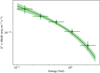 |
Fig. 16. Simulated spectrum of HD 93129A for an extrapolated FL8Y power law with an Ecut = 2 TeV cut-off input spectrum. A 50 h observation was used for the simulation. |
5. Discussion and conclusions
We have presented an overview of the current observations of γ-ray binaries and illustrated the capability of the CTA to study the spectral and timing properties of these sources. The full list of the considered sources with the basic parameters of the hosting systems are summarised in Tables 1 and 3.
Despite dedicated observations with all modern VHE facilities (H.E.S.S., MAGIC, VERITAS, and HAWC), the statistics of the VHE data is still poor. At best, γ-ray binaries can only be marginally detected at VHE in a few hours, whereas for some of them, variability on timescales as short as ≈30 min is observed in the X-ray and HE bands (e.g. Chernyakova et al. 2009; Johnson et al. 2018). Measuring the basic spectral parameters (e.g. spectral slope) in the TeV band requires even longer exposure times. The studies of more complex parameters, such as spectral curvature, orbital variations of the cut-off energy, orbit-to-orbit variability, and short timescale variability are in most cases beyond the current sensitivity limits. This complicates a comparison of TeV and lower energy (radio to GeV) data where all the variabilites listed above are known to be present. The large uncertainty in the study of simultaneous variability prevents a firm confirmation of whether the same relativistic particle population is responsible for the broad-band emission. See also Paredes & Bordas (2019) for a broader list of open questions.
The unprecedented sensitivity of the CTA will in most cases enable studying the spectral evolution of binaries such as PSR B1259−63, LS 5039, LS I +61° 303, and HESS J0632+057 on time scales as short as 30 min, which is comparable to the variability observed in X-rays. This will address the statistics-related issues of the current-generation instruments described above and provide input data for theories describing details of particle acceleration. For example, the presence of clumps in a stellar wind is thought to modify the wind-wind collision shock structure and affect the efficiency of particle acceleration in relativistic hydrodynamical simulations (see e.g. Paredes-Fortuny et al. 2015; Dubus et al. 2015). The CTA observations of the short time-scale variability in γ-ray binaries may allow the properties of the clumps to be assessed. For example, their scale-distrubution can be reconstructed using an approach similar to the one applied by Chernyakova et al. (2017) to X-ray data.
Studies of the orbital variability of the high-energy spectral cut-off can identify the environmental parameters that lead to the most efficient particle acceleration. Current observations are unable to constrain the highest energy of relativistic particles for most of the known binaries. Only in the case of LS 5039 is the cut-off energy Ecut = 6.6 TeV measured close to the inferior conjunction (Mariaud et al. 2015). Under the assumption that the γ-ray emitter is a jet-like structure, Khangulyan et al. (2008b) built a model that reproduced the spectral states of the system near the inferior and exterior conjunctions. However, to test this model and constrain the physical properties of the source, observations tha can provide detailed energy spectra for narrow orbital phase intervals (Δφ < 0.1) are needed. As the simulations presented in Fig. 1 and in Sect. 3 show, the CTA will be easily able to undertake such observations. Below we briefly summarize what CTA could do for γ-ray binaries and outline the questions that can be addressed.
PSR B1259−63. CTA observation around the periastron passage will allow studying the spectral variability on a 30 min timescale at a level of better than 5%. This will finally answer the question of whether the TeV light curve also has two peaks around periastron, similar to radio and X-rays, and enable us to study the spectral evolution caused by gamma-gamma absorption. Accompanied with simultaneous multi-wavelength observations. the CTA data will allow us to test numerous models of particle acceleration in the system, the composition of the pulsar wind, and the details of the interaction of the pulsar wind with the disc of the Be star that cause the still unexplained GeV flare.
LS I +61° 303, LS 5039, and 1FGL J1018.6−5856. Spectral studies with an accuracy of better than 10% on a few-hour timescale will become possible, which is less than 1% of the orbital period of these systems. CTA observations will also study the short timescale variability down to 30 min, which will allow for a direct multi-wavelength comparison. Detailed reconstruction of the broad-band spectral variability on short and orbital timescales will allow us to test existing models and reconstruct the details of the geometry and physical conditions of the emission region.
HESS J0632+057. CTA observations will allow accurately monitoring the high-energy slope and energy break throughout the orbit. Fifty hours of observation will allow us to reconstruct the flux and slope of the source with an accuracy better than 3% and the position of the spectral break with an accuracy of 10%.
This will enable us to distinguish the current theoretical models, to understand if the compact object in the system undergoes accretion close to periastron (flip-flop model), or if the observed two-peak orbital light curve is due to the inclination of the Be star disc to the orbital plane.
HESS J1832−093. For less thoroughly studied binary systems like this, CTA observations will be crucial for understanding their nature. CTA observations of HESS J1832−093 with the improved angular resolution of the telescope will place further constraints on the extent of the TeV source. This information, accompanied with the detailed measurements of the spectral variability of the source on different timescales, will help to ascertain the nature of the system and determine whether it is indeed a γ-ray binary.
LMC P3. The CTA sensitivity will be high enough to study the nightly averaged spectral evolution of the source oir the first time with an accuracy better than 10% throughout the orbit. This will place clear constraints on the geometry of the system and on the details of the physical processes governing the observed emission. It will also contribute to the development of a consistent model for the multi-wavelength emission.
η Carinae and other CWBs. We demonstrated that the CTA will be able to greatly advance the study of high-energy emission for CWBs. At the time of writing, TeV emission was detected from only one CWB: η Car. With the CTA it will be possible to probe the spectrum and variability of η Car above 30 GeV throughout the orbit with a resolution of a few days. This will allow the nature of the high-energy component to be established and constrain the geometry of the shock at the core of the system. For other CWB candidates, of which γ2 Vel and HD 93129A are the most prominent, the CTA sensitivity will be high enough to probe the presence of TeV emission.
We have verified that results obtained have a negligible dependency on the choice of the Galactic diffuse background model.
Acknowledgments
We gratefully acknowledge financial support from the agencies and organizations listed here: http://www.cta-observatory.org/consortium_acknowledgments. This research made use of ctools, a community-developed analysis package for Imaging Air Cherenkov Telescope data. ctools is based on GammaLib, a community-developed toolbox for the high-level analysis of astronomical γ-ray data. This research has made use of the CTA instrument response functions provided by the CTA Consortium and Observatory, see https://www.cta-observatory.org/science/cta-performance/ (version prod3b-v1) for more details. The authors acknowledge support by the state of Baden-Württemberg through bwHPC. This work was supported by the Carl-Zeiss Stiftung through the grant “Hochsensitive Nachweistechnik zur Erforschung des unsichtbaren Universums” to the Kepler Center für Astro- und Teilchenphysik at the University of Tübingen. PR, GP, FC and SV acknowledge contribution from the grant INAF CTA–SKA, “Towards the SKA and CTA era: discovery, localisation, and physics of transient sources” (PI M. Giroletti). LS acknowledges financial support of the ERDF under the Spanish MINECO (FPA2015-68378-P and FPA2017-82729-C6-3-R). JMP and MR acknowledge support by the Spanish Ministerio de Economía, Industria y Competitividad (MINEICO/FEDER, UE) under grants FPA2015-69210-C6-2-R, AYA2016-76012-C3-1- P, MDM-2014-0369 of ICCUB (Unidad de Excelencia ‘María de Maeztu’) and the Catalan DEC grant 2017 SGR 643. PLE and JM also acknowledge support by MINECO/FEDER, UE under grant AYA2016-76012-C3-3-P and by the Consejería de Economía, Innovación, Ciencia y Empleo of Junta de Andalucía under research group FQM-322. MC acknowledge SFI/HEA Irish Centre for High-End Computing (ICHEC) for the provision of computational facilities and support.
References
- Abdo, A. A., Ackermann, M., Ajello, M., et al. 2009, ApJ, 701, L123 [NASA ADS] [CrossRef] [Google Scholar]
- Abdo, A. A., Ackermann, M., Ajello, M., et al. 2010, ApJ, 723, 649 [NASA ADS] [CrossRef] [Google Scholar]
- Abdo, A. A., Ackermann, M., Ajello, M., et al. 2011, ApJ, 736, L11 [NASA ADS] [CrossRef] [Google Scholar]
- Abeysekara, A. U., Albert, A., Alfaro, R., et al. 2018, Nature, 562, 82 [NASA ADS] [CrossRef] [Google Scholar]
- Abraham, Z., Falceta-Gonçalves, D., & Beaklini, P. P. B. 2014, ApJ, 791, 95 [NASA ADS] [CrossRef] [Google Scholar]
- Acciari, V. A., Beilicke, M., Blaylock, G., et al. 2008, ApJ, 679, 1427 [NASA ADS] [CrossRef] [Google Scholar]
- Acero, F., Ackermann, M., Ajello, M., et al. 2015, ApJS, 218, 23 [Google Scholar]
- Ackermann, M., Ajello, M., Ballet, J., et al. 2013, ApJ, 773, L35 [NASA ADS] [CrossRef] [Google Scholar]
- Aharonian, F., Akhperjanian, A. G., Aye, K.-M., et al. 2005a, A&A, 442, 1 [NASA ADS] [CrossRef] [EDP Sciences] [Google Scholar]
- Aharonian, F., Akhperjanian, A. G., Aye, K.-M., et al. 2005b, Science, 309, 746 [NASA ADS] [CrossRef] [PubMed] [Google Scholar]
- Aharonian, F., Akhperjanian, A. G., Bazer-Bachi, A. R., et al. 2006, A&A, 457, 899 [NASA ADS] [CrossRef] [EDP Sciences] [Google Scholar]
- Aharonian, F. A., Akhperjanian, A. G., Bazer-Bachi, A. R., et al. 2007, A&A, 469, L1 [NASA ADS] [CrossRef] [EDP Sciences] [Google Scholar]
- Aharonian, F., Akhperjanian, A. G., Anton, G., et al. 2009, A&A, 507, 389 [NASA ADS] [CrossRef] [EDP Sciences] [Google Scholar]
- Ahnen, M. L., Ansoldi, S., Antonelli, L. A., et al. 2016, A&A, 591, A76 [NASA ADS] [CrossRef] [EDP Sciences] [Google Scholar]
- Albert, J., Aliu, E., Anderhub, H., et al. 2006, Science, 312, 1771 [NASA ADS] [CrossRef] [PubMed] [Google Scholar]
- Albert, J., Aliu, E., Anderhub, H., et al. 2007, ApJ, 665, L51 [NASA ADS] [CrossRef] [Google Scholar]
- Albert, J., Aliu, E., Anderhub, H., et al. 2009, ApJ, 693, 303 [NASA ADS] [CrossRef] [Google Scholar]
- Aleksić, J., Alvarez, E. A., Antonelli, L. A., et al. 2012a, Astropart. Phys., 35, 435 [NASA ADS] [CrossRef] [Google Scholar]
- Aleksić, J., Alvarez, E. A., Antonelli, L. A., et al. 2012b, ApJ, 746, 80 [NASA ADS] [CrossRef] [Google Scholar]
- Aleksić, J., Alvarez, E. A., Antonelli, L. A., et al. 2012c, ApJ, 754, L10 [NASA ADS] [CrossRef] [Google Scholar]
- Aliu, E., Archambault, S., Behera, B., et al. 2013, ApJ, 779, 88 [NASA ADS] [CrossRef] [Google Scholar]
- Aliu, E., Archambault, S., Aune, T., et al. 2014, ApJ, 780, 168 [NASA ADS] [CrossRef] [Google Scholar]
- An, H., & Romani, R. W. 2017, ApJ, 838, 145 [NASA ADS] [CrossRef] [Google Scholar]
- An, H., Bellm, E., Bhalerao, V., et al. 2015, ApJ, 806, 166 [NASA ADS] [CrossRef] [Google Scholar]
- Anderhub, H., Antonelli, L. A., Antoranz, P., et al. 2009, ApJ, 706, L27 [NASA ADS] [CrossRef] [Google Scholar]
- Aragona, C., McSwain, M. V., Grundstrom, E. D., et al. 2009, ApJ, 698, 514 [NASA ADS] [CrossRef] [Google Scholar]
- Aragona, C., McSwain, M. V., & De Becker, M. 2010, ApJ, 724, 306 [NASA ADS] [CrossRef] [Google Scholar]
- Balbo, M., & Walter, R. 2017, A&A, 603, A111 [NASA ADS] [CrossRef] [EDP Sciences] [Google Scholar]
- Barthelmy, S. D., Baumgartner, W., Cummings, J., et al. 2008, GRB Coordinates Network, 8215 [Google Scholar]
- Bednarek, W., & Pabich, J. 2011, A&A, 530, A49 [NASA ADS] [CrossRef] [EDP Sciences] [Google Scholar]
- Bodaghee, A., Tomsick, J. A., Pottschmidt, K., et al. 2013, ApJ, 775, 98 [NASA ADS] [CrossRef] [Google Scholar]
- Bongiorno, S. D., Falcone, A. D., Stroh, M., et al. 2011, ApJ, 737, L11 [NASA ADS] [CrossRef] [Google Scholar]
- Bordas, P., Yang, R., Kafexhiu, E., & Aharonian, F. 2015, ApJ, 807, L8 [NASA ADS] [CrossRef] [Google Scholar]
- Böttcher, M., & Dermer, C. D. 2005, ApJ, 634, L81 [NASA ADS] [CrossRef] [Google Scholar]
- Caliandro, G. A., Cheung, C. C., Li, J., et al. 2015, ApJ, 811, 68 [NASA ADS] [CrossRef] [Google Scholar]
- Casares, J., Ribas, I., Paredes, J. M., Martí, J., & Allende Prieto, C. 2005, MNRAS, 360, 1105 [NASA ADS] [CrossRef] [Google Scholar]
- Casares, J., Ribó, M., Ribas, I., et al. 2012, MNRAS, 421, 1103 [NASA ADS] [CrossRef] [Google Scholar]
- Casares, J., Negueruela, I., Ribó, M., et al. 2014, Nature, 505, 378 [NASA ADS] [CrossRef] [Google Scholar]
- Chang, Z., Zhang, S., Ji, L., et al. 2016, MNRAS, 463, 495 [NASA ADS] [CrossRef] [Google Scholar]
- Chapman, J. M., Leitherer, C., Koribalski, B., Bouter, R., & Storey, M. 1999, ApJ, 518, 890 [NASA ADS] [CrossRef] [Google Scholar]
- Chernyakova, M., Neronov, A., Aharonian, F., Uchiyama, Y., & Takahashi, T. 2009, MNRAS, 397, 2123 [NASA ADS] [CrossRef] [Google Scholar]
- Chernyakova, M., Neronov, A., Molkov, S., et al. 2012, ApJ, 747, L29 [NASA ADS] [CrossRef] [Google Scholar]
- Chernyakova, M., Abdo, A. A., Neronov, A., et al. 2014, MNRAS, 439, 432 [NASA ADS] [CrossRef] [Google Scholar]
- Chernyakova, M., Neronov, A., van Soelen, B., et al. 2015, MNRAS, 454, 1358 [NASA ADS] [CrossRef] [Google Scholar]
- Chernyakova, M., Babyk, I., Malyshev, D., et al. 2017, MNRAS, 470, 1718 [NASA ADS] [CrossRef] [Google Scholar]
- Cominsky, L., Roberts, M., & Johnston, S. 1994, ApJ, 427, 978 [NASA ADS] [CrossRef] [Google Scholar]
- Corbet, R. H. D., Chomiuk, L., Coe, M. J., et al. 2016, ApJ, 829, 105 [NASA ADS] [CrossRef] [Google Scholar]
- Corbet, R. H. D., Chomiuk, L., Coe, M. J., et al. 2019, ApJ, 884, 93 [NASA ADS] [CrossRef] [Google Scholar]
- Corcoran, M. F. 2005, AJ, 129, 2018 [NASA ADS] [CrossRef] [Google Scholar]
- Corcoran, M. F., Ishibashi, K., Swank, J. H., & Petre, R. 2001, ApJ, 547, 1034 [NASA ADS] [CrossRef] [Google Scholar]
- Corcoran, M. F., Hamaguchi, K., Liburd, J. K., et al. 2015, ArXiv e-prints [arXiv:1507.07961] [Google Scholar]
- CTA Consortium 2017, ArXiv e-prints [arXiv:1709.05434] [Google Scholar]
- CTA Consortium 2019, Science with the Cherenkov Telescope Array (Singapore: World Scientific Publishing Co., Pte. Ltd.) [Google Scholar]
- Damineli, A., Kaufer, A., Wolf, B., et al. 2000, ApJ, 528, L101 [NASA ADS] [CrossRef] [PubMed] [Google Scholar]
- Damineli, A., Hillier, D. J., Corcoran, M. F., et al. 2008, MNRAS, 384, 1649 [NASA ADS] [CrossRef] [Google Scholar]
- De Becker, M., Benaglia, P., Romero, G. E., & Peri, C. S. 2017, A&A, 600, A47 [NASA ADS] [CrossRef] [EDP Sciences] [Google Scholar]
- del Palacio, S., Bosch-Ramon, V., Romero, G. E., & Benaglia, P. 2016, A&A, 591, A139 [NASA ADS] [CrossRef] [EDP Sciences] [Google Scholar]
- del Palacio, S., Bosch-Ramon, V., Romero, G. E., & Benaglia, P. 2017, in 6th International Symposium on High Energy Gamma-Ray Astronomy, AIP Conf. Ser., 1792, 040027 [Google Scholar]
- De Marco, O., & Schmutz, W. 1999, A&A, 345, 163 [NASA ADS] [Google Scholar]
- Dougherty, S. M., Pittard, J. M., Kasian, L., et al. 2003, A&A, 409, 217 [NASA ADS] [CrossRef] [EDP Sciences] [Google Scholar]
- Dubus, G. 2006, A&A, 451, 9 [NASA ADS] [CrossRef] [EDP Sciences] [Google Scholar]
- Dubus, G. 2013, A&ARv, 21, 64 [NASA ADS] [CrossRef] [Google Scholar]
- Dubus, G., Cerutti, B., & Henri, G. 2008, A&A, 477, 691 [NASA ADS] [CrossRef] [EDP Sciences] [Google Scholar]
- Dubus, G., Lamberts, A., & Fromang, S. 2015, A&A, 581, A27 [NASA ADS] [CrossRef] [EDP Sciences] [Google Scholar]
- Dubus, G., Guillard, N., Petrucci, P.-O., & Martin, P. 2017, A&A, 608, A59 [NASA ADS] [CrossRef] [EDP Sciences] [Google Scholar]
- Eger, P., Laffon, H., Bordas, P., et al. 2016, MNRAS, 457, 1753 [NASA ADS] [CrossRef] [Google Scholar]
- Eichler, D., & Usov, V. 1993, ApJ, 402, 271 [NASA ADS] [CrossRef] [Google Scholar]
- Falceta-Goncalves, D. 2015, in Wolf-Rayet Stars: Proceedings of an International Workshop held in Potsdam, Germany, 1–5 June 2015, eds. W. R. Hamann, A. Sander, & H. Todt (Potsdam: Universitätsverlag Potsdam), 289 [Google Scholar]
- Falceta-Gonçalves, D., & Abraham, Z. 2012, MNRAS, 423, 1562 [NASA ADS] [CrossRef] [Google Scholar]
- Falceta-Gonçalves, D., Jatenco-Pereira, V., & Abraham, Z. 2005, MNRAS, 357, 895 [NASA ADS] [CrossRef] [Google Scholar]
- Falcone, A. D., Grube, J., Hinton, J., et al. 2010, ApJ, 708, L52 [NASA ADS] [CrossRef] [Google Scholar]
- Farnier, C., Walter, R., & Leyder, J.-C. 2011, A&A, 526, A57 [NASA ADS] [CrossRef] [EDP Sciences] [Google Scholar]
- Fermi LAT Collaboration (Ackermann, M., et al.) 2012, Science, 335, 189 [NASA ADS] [CrossRef] [Google Scholar]
- Gagné, M., Fehon, G., Savoy, M. R., et al. 2011, ApJS, 194, 5 [NASA ADS] [CrossRef] [EDP Sciences] [Google Scholar]
- Gomez, H. L., Vlahakis, C., Stretch, C. M., et al. 2010, MNRAS, 401, L48 [NASA ADS] [CrossRef] [Google Scholar]
- Gregory, P. C. 2002, ApJ, 575, 427 [NASA ADS] [CrossRef] [Google Scholar]
- Gregory, P. C., & Taylor, A. R. 1978, Nature, 272, 704 [NASA ADS] [CrossRef] [Google Scholar]
- Gregory, P. C., Taylor, A. R., Crampton, D., et al. 1979, AJ, 84, 1030 [NASA ADS] [CrossRef] [Google Scholar]
- Grimm, H.-J., Gilfanov, M., & Sunyaev, R. 2002, A&A, 391, 923 [NASA ADS] [CrossRef] [EDP Sciences] [Google Scholar]
- Groh, J. H., Hillier, D. J., Madura, T. I., & Weigelt, G. 2012, MNRAS, 423, 1623 [NASA ADS] [CrossRef] [Google Scholar]
- Hadasch, D., Torres, D. F., Tanaka, T., et al. 2012, ApJ, 749, 54 [NASA ADS] [CrossRef] [Google Scholar]
- Hermsen, W., Swanenburg, B. N., Bignami, G. F., et al. 1977, Nature, 269, 494 [NASA ADS] [CrossRef] [Google Scholar]
- H.E.S.S. Collaboration (Abramowski, A., et al.) 2012a, A&A, 541, A5 [NASA ADS] [CrossRef] [EDP Sciences] [Google Scholar]
- H.E.S.S. Collaboration (Abramowski, A., et al.) 2012b, MNRAS, 424, 128 [NASA ADS] [CrossRef] [Google Scholar]
- H.E.S.S. Collaboration (Abramowski, A., et al.) 2013, A&A, 551, A94 [NASA ADS] [CrossRef] [EDP Sciences] [Google Scholar]
- H.E.S.S. Collaboration (Abramowski, A.) 2015a, A&A, 577, A131 [NASA ADS] [CrossRef] [EDP Sciences] [Google Scholar]
- H.E.S.S. Collaboration (Abramowski, A., et al.) 2015b, MNRAS, 446, 1163 [NASA ADS] [Google Scholar]
- H.E.S.S. Collaboration (Abdalla, H., et al.) 2018, A&A, 610, L17 [NASA ADS] [CrossRef] [EDP Sciences] [Google Scholar]
- Hillier, D. J., Davidson, K., Ishibashi, K., & Gull, T. 2001, ApJ, 553, 837 [NASA ADS] [CrossRef] [Google Scholar]
- Hinton, J. A., Skilton, J. L., Funk, S., et al. 2009, ApJ, 690, L101 [NASA ADS] [CrossRef] [Google Scholar]
- Ho, W. C. G., Ng, C.-Y., Lyne, A. G., et al. 2017, MNRAS, 464, 1211 [NASA ADS] [CrossRef] [Google Scholar]
- Jaron, F., & Massi, M. 2014, A&A, 572, A105 [NASA ADS] [CrossRef] [EDP Sciences] [Google Scholar]
- Johnston, S., Ball, L., Wang, N., & Manchester, R. N. 2005, MNRAS, 358, 1069 [NASA ADS] [CrossRef] [Google Scholar]
- Johnson, T. J., Wood, K. S., Ray, P. S., Kerr, M. T., & Cheung, C. C. 2017, ATel, 11028 [Google Scholar]
- Johnson, T. J., Wood, K. S., Kerr, M., et al. 2018, ApJ, 863, 27 [NASA ADS] [CrossRef] [Google Scholar]
- Johnston, S., Lyne, A. G., Manchester, R. N., et al. 1992a, MNRAS, 255, 401 [NASA ADS] [CrossRef] [Google Scholar]
- Johnston, S., Manchester, R. N., Lyne, A. G., et al. 1992b, ApJ, 387, L37 [NASA ADS] [CrossRef] [Google Scholar]
- Johnston, S., Manchester, R. N., Lyne, A. G., Nicastro, L., & Spyromilio, J. 1994, MNRAS, 268, 430 [NASA ADS] [Google Scholar]
- Johnston, S., Wex, N., Nicastro, L., Manchester, R. N., & Lyne, A. G. 2001, MNRAS, 326, 643 [NASA ADS] [CrossRef] [Google Scholar]
- Kar, P., & VERITAS Collaboration 2015, in 34th International Cosmic Ray Conference (ICRC2015), Proc. Sci., 34, 818 [Google Scholar]
- Kar, P., & VERITAS Collaboration 2017, Int. Cosmic Ray Conf., 35, 712 [Google Scholar]
- Kerschhaggl, M. 2011, A&A, 525, A80 [NASA ADS] [CrossRef] [EDP Sciences] [Google Scholar]
- Khangulyan, D., Hnatic, S., Aharonian, F., & Bogovalov, S. 2007, MNRAS, 380, 320 [NASA ADS] [CrossRef] [Google Scholar]
- Khangulyan, D. V., Aharonian, F. A., Bogovalov, S. V., Koldoba, A. V., & Ustyugova, G. V. 2008a, Int. J. Mod. Phys. D, 17, 1909 [NASA ADS] [CrossRef] [Google Scholar]
- Khangulyan, D., Aharonian, F., & Bosch-Ramon, V. 2008b, MNRAS, 383, 467 [NASA ADS] [CrossRef] [Google Scholar]
- Knödlseder, J., Mayer, M., Deil, C., et al. 2016, A&A, 593, A1 [NASA ADS] [CrossRef] [EDP Sciences] [Google Scholar]
- Leser, E. F. 2017, ICRC Presentation Available at https://indico.snu.ac.kr/indico/event/15/session/6/contribution/371/material/slides/0.pdf [Google Scholar]
- Leyder, J.-C., Walter, R., & Rauw, G. 2008, A&A, 477, L29 [Google Scholar]
- Li, J., Torres, D. F., & Zhang, S. 2014, ApJ, 785, L19 [NASA ADS] [CrossRef] [Google Scholar]
- Li, J., Torres, D. F., Cheng, K.-S., et al. 2017, ApJ, 846, 169 [NASA ADS] [CrossRef] [Google Scholar]
- Lyne, A. G., Stappers, B. W., Keith, M. J., et al. 2015, MNRAS, 451, 581 [NASA ADS] [CrossRef] [Google Scholar]
- Maier, G., & VERITAS Collaboration 2015, Proc. 34th Int. Cosmic Ray Conf. (ICRC2015), 754 [Google Scholar]
- Maíz Apellániz, J., Sana, H., Barbá, R. H., Le Bouquin, J.-B., & Gamen, R. C. 2017, MNRAS, 464, 3561 [NASA ADS] [CrossRef] [Google Scholar]
- Malyshev, D., & Chernyakova, M. 2016, MNRAS, 463, 3074 [NASA ADS] [CrossRef] [Google Scholar]
- Malyshev, D., Zdziarski, A. A., & Chernyakova, M. 2013, MNRAS, 434, 2380 [NASA ADS] [CrossRef] [Google Scholar]
- Malyshev, D., Chernyakova, M., Santangelo, A., & Pühlhofer, G. 2017, Astron. Nachr., unpublished [arXiv:1711.05001] [Google Scholar]
- Maraschi, L., & Treves, A. 1981, MNRAS, 194, 1P [NASA ADS] [CrossRef] [Google Scholar]
- Marcote, B., Ribó, M., Paredes, J. M., Mao, M. Y., & Edwards, P. G. 2018, A&A, 619, A26 [NASA ADS] [CrossRef] [EDP Sciences] [Google Scholar]
- Mariaud, C., Bordas, P., Aharonian, F., et al. 2015, ArXiv e-prints [arXiv:1509.05791] [Google Scholar]
- Martí, J., Paredes, J. M., & Ribó, M. 1998, A&A, 338, L71 [NASA ADS] [Google Scholar]
- Martí, J., Luque-Escamilla, P. L., Paredes, J. M., et al. 2017, A&A, 598, A81 [NASA ADS] [CrossRef] [EDP Sciences] [Google Scholar]
- Massi, M., & Jaron, F. 2013, A&A, 554, A105 [NASA ADS] [CrossRef] [EDP Sciences] [Google Scholar]
- Massi, M., & Torricelli-Ciamponi, G. 2016, A&A, 585, A123 [NASA ADS] [CrossRef] [EDP Sciences] [Google Scholar]
- Massi, M., Paredes, J. M., Estalella, R., & Felli, M. 1993, A&A, 269, 249 [NASA ADS] [CrossRef] [Google Scholar]
- Massi, M., Ribó, M., Paredes, J. M., et al. 2004, A&A, 414, L1 [NASA ADS] [CrossRef] [EDP Sciences] [Google Scholar]
- Massi, M., Jaron, F., & Hovatta, T. 2015, A&A, 575, L9 [NASA ADS] [CrossRef] [EDP Sciences] [Google Scholar]
- Massi, M., Migliari, S., & Chernyakova, M. 2017, MNRAS, 468, 3689 [NASA ADS] [CrossRef] [Google Scholar]
- McSwain, M. V., Gies, D. R., Huang, W., et al. 2004, ApJ, 600, 927 [NASA ADS] [CrossRef] [Google Scholar]
- McSwain, M. V., Chernyakova, M., Malishev, D., De Becker, M., & Williams, S. 2013, ArXiv e-prints [arXiv:1303.2018] [Google Scholar]
- Mendelson, H., & Mazeh, T. 1989, MNRAS, 239, 733 [NASA ADS] [Google Scholar]
- Miller-Jones, J. C. A., Deller, A. T., Shannon, R. M., et al. 2018, MNRAS, 479, 4849 [NASA ADS] [CrossRef] [Google Scholar]
- Mirabel, I. F., & Rodríguez, L. F. 1998, Nature, 392, 673 [NASA ADS] [CrossRef] [Google Scholar]
- Moldón, J., Johnston, S., Ribó, M., Paredes, J. M., & Deller, A. T. 2011, ApJ, 732, L10 [NASA ADS] [CrossRef] [Google Scholar]
- Moldón, J., Ribó, M., & Paredes, J. M. 2012, A&A, 548, A103 [NASA ADS] [CrossRef] [EDP Sciences] [Google Scholar]
- Monageng, I. M., McBride, V. A., Townsend, L. J., et al. 2017, ApJ, 847, 68 [NASA ADS] [CrossRef] [Google Scholar]
- Mori, K., Gotthelf, E. V., Hailey, C. J., et al. 2017, ApJ, 848, 80 [NASA ADS] [CrossRef] [Google Scholar]
- Moritani, Y., Okazaki, A. T., Carciofi, A. C., et al. 2015, ApJ, 804, L32 [NASA ADS] [CrossRef] [Google Scholar]
- Moritani, Y., Kawano, T., Chimasu, S., et al. 2018, PASJ, 70, 61 [NASA ADS] [Google Scholar]
- Motch, C., Haberl, F., Dennerl, K., Pakull, M., & Janot-Pacheco, E. 1997, A&A, 323, 853 [NASA ADS] [Google Scholar]
- Munar-Adrover, P., Sabatini, S., Piano, G., et al. 2016, ApJ, 829, 101 [NASA ADS] [CrossRef] [Google Scholar]
- Napoli, V. J., McSwain, M. V., Marsh Boyer, A. N., & Roettenbacher, R. M. 2011, PASP, 123, 1262 [NASA ADS] [CrossRef] [Google Scholar]
- Negueruela, I., Okazaki, A. T., Fabregat, J., et al. 2001, A&A, 369, 117 [NASA ADS] [CrossRef] [EDP Sciences] [Google Scholar]
- Negueruela, I., Ribó, M., Herrero, A., et al. 2011, ApJ, 732, L11 [NASA ADS] [CrossRef] [Google Scholar]
- Neronov, A., & Chernyakova, M. 2007, Ap&SS, 309, 253 [NASA ADS] [CrossRef] [Google Scholar]
- Neronov, A., & Chernyakova, M. 2008, ApJ, 672, L123 [NASA ADS] [CrossRef] [Google Scholar]
- North, J. R., Tuthill, P. G., Tango, W. J., & Davis, J. 2007, MNRAS, 377, 415 [NASA ADS] [CrossRef] [Google Scholar]
- Nösel, S., Sharma, R., Massi, M., Cimò, G., & Chernyakova, M. 2018, MNRAS, 476, 2516 [NASA ADS] [CrossRef] [Google Scholar]
- Ohm, S., Zabalza, V., Hinton, J. A., & Parkin, E. R. 2015, MNRAS, 449, L132 [NASA ADS] [CrossRef] [Google Scholar]
- Okazaki, A. T., Owocki, S. P., Russell, C. M. P., & Corcoran, M. F. 2008, MNRAS, 388, L39 [NASA ADS] [CrossRef] [MathSciNet] [Google Scholar]
- Panagiotou, C., & Walter, R. 2018, A&A, 610, A37 [NASA ADS] [CrossRef] [EDP Sciences] [Google Scholar]
- Paredes, J. M., & Bordas, P. 2019, ArXiv e-prints [arXiv:1902.09898] [Google Scholar]
- Paredes, J. M., Marziani, P., Marti, J., et al. 1994, A&A, 288, 519 [NASA ADS] [Google Scholar]
- Paredes, J. M., Marti, J., Peracaula, M., & Ribo, M. 1997, A&A, 320, L25 [NASA ADS] [Google Scholar]
- Paredes, J. M., Massi, M., Estalella, R., & Peracaula, M. 1998, A&A, 335, 539 [NASA ADS] [Google Scholar]
- Paredes, J. M., Martí, J., Ribó, M., & Massi, M. 2000, Science, 288, 2340 [NASA ADS] [CrossRef] [PubMed] [Google Scholar]
- Paredes-Fortuny, X., Bosch-Ramon, V., Perucho, M., & Ribó, M. 2015, A&A, 574, A77 [NASA ADS] [CrossRef] [EDP Sciences] [Google Scholar]
- Park, N., & VERITAS Collaboration 2015, in 34th Int. Cosmic Ray Conf. (ICRC2015), eds. A. S. Borisov, V. G. Denisova, Z. M. Guseva, et al., 34, 771 [Google Scholar]
- Parkin, E. R., Pittard, J. M., Corcoran, M. F., Hamaguchi, K., & Stevens, I. R. 2009, MNRAS, 394, 1758 [NASA ADS] [CrossRef] [Google Scholar]
- Parkin, E. R., Pittard, J. M., Corcoran, M. F., & Hamaguchi, K. 2011, ApJ, 726, 105 [NASA ADS] [CrossRef] [Google Scholar]
- Pavlov, G. G., Chang, C., & Kargaltsev, O. 2011, ApJ, 730, 2 [NASA ADS] [CrossRef] [Google Scholar]
- Pavlov, G. G., Hare, J., Kargaltsev, O., Rangelov, B., & Durant, M. 2015, ApJ, 806, 192 [NASA ADS] [CrossRef] [Google Scholar]
- Pietrzyński, G., Graczyk, D., Gieren, W., et al. 2013, Nature, 495, 76 [NASA ADS] [CrossRef] [PubMed] [Google Scholar]
- Pittard, J. M., & Corcoran, M. F. 2002, A&A, 383, 636 [NASA ADS] [CrossRef] [EDP Sciences] [Google Scholar]
- Pshirkov, M. S. 2016, MNRAS, 457, L99 [NASA ADS] [CrossRef] [Google Scholar]
- Ray, P. S., Foster, R. S., Waltman, E. B., Tavani, M., & Ghigo, F. D. 1997, ApJ, 491, 381 [NASA ADS] [CrossRef] [Google Scholar]
- Reimer, A., Pohl, M., & Reimer, O. 2006, ApJ, 644, 1118 [NASA ADS] [CrossRef] [Google Scholar]
- Reitberger, K., Reimer, O., Reimer, A., et al. 2012, A&A, 544, A98 [NASA ADS] [CrossRef] [EDP Sciences] [Google Scholar]
- Reitberger, K., Kissmann, R., Reimer, A., & Reimer, O. 2017, ApJ, 847, 40 [NASA ADS] [CrossRef] [Google Scholar]
- Ribó, M., Paredes, J. M., Romero, G. E., et al. 2002, A&A, 384, 954 [NASA ADS] [CrossRef] [EDP Sciences] [Google Scholar]
- Rocha da Silva, G., Falceta-Gonçalves, D., Kowal, G., & de Gouveia Dal Pino, E. M. 2015, MNRAS, 446, 104 [NASA ADS] [CrossRef] [Google Scholar]
- Romoli, C., Bordas, P., Mariaud, C., Murach, T., & H.E.S.S. Collaboration 2017, 35th Int. Cosmic Ray Conf., Proc. Science, 301, 675 [Google Scholar]
- Sabatini, S., Striani, E., Verrecchia, F., et al. 2010, ATel, 2715 [Google Scholar]
- Saha, L., Chitnis, V. R., Shukla, A., Rao, A. R., & Acharya, B. S. 2016, ApJ, 823, 134 [NASA ADS] [CrossRef] [Google Scholar]
- Sarty, G. E., Szalai, T., Kiss, L. L., et al. 2011, MNRAS, 411, 1293 [NASA ADS] [CrossRef] [Google Scholar]
- Schlenstedt, S. 2017, in 6th International Symposium on High Energy Gamma-Ray Astronomy, AIP Conf. Ser., 1792, 040023 [Google Scholar]
- Schmutz, W., Schweickhardt, J., Stahl, O., et al. 1997, A&A, 328, 219 [NASA ADS] [Google Scholar]
- Shannon, R. M., Johnston, S., & Manchester, R. N. 2014, MNRAS, 437, 3255 [NASA ADS] [CrossRef] [Google Scholar]
- Sidoli, L., Pellizzoni, A., Vercellone, S., et al. 2006, A&A, 459, 901 [NASA ADS] [CrossRef] [EDP Sciences] [Google Scholar]
- Skilton, J. L., Pandey-Pommier, M., Hinton, J. A., et al. 2009, MNRAS, 399, 317 [NASA ADS] [CrossRef] [Google Scholar]
- Smith, N., Gehrz, R. D., Hinz, P. M., et al. 2003, AJ, 125, 1458 [NASA ADS] [CrossRef] [Google Scholar]
- Smith, A., Kaaret, P., Holder, J., et al. 2009, ApJ, 693, 1621 [NASA ADS] [CrossRef] [Google Scholar]
- Strader, J., Chomiuk, L., Cheung, C. C., Salinas, R., & Peacock, M. 2015, ApJ, 813, L26 [NASA ADS] [CrossRef] [Google Scholar]
- Sushch, I., & van Soelen, B. 2017, ApJ, 837, 175 [NASA ADS] [CrossRef] [Google Scholar]
- Takahashi, T., Kishishita, T., Uchiyama, Y., et al. 2009, ApJ, 697, 592 [NASA ADS] [CrossRef] [Google Scholar]
- Takata, J., Okazaki, A. T., Nagataki, S., et al. 2012, ApJ, 750, 70 [NASA ADS] [CrossRef] [Google Scholar]
- Tam, P. H. T., Huang, R. H. H., Takata, J., et al. 2011, ApJ, 736, L10 [NASA ADS] [CrossRef] [Google Scholar]
- Tam, P. H. T., Li, K. L., Takata, J., et al. 2015, ApJ, 798, L26 [NASA ADS] [CrossRef] [Google Scholar]
- Tam, P.-H. T., He, X., Sarathi Pal, P., & Cui, Y. 2018, ApJ, 862, 8 [Google Scholar]
- Tatischeff, V., Terrier, R., & Lebrun, F. 2004, in 5th INTEGRAL Workshop on the INTEGRAL Universe, eds. V. Schoenfelder, G. Lichti, & C. Winkler, ESA Spec. Publ., 552, 409 [NASA ADS] [Google Scholar]
- Tavani, M., Grove, J. E., Purcell, W., et al. 1996, A&AS, 120, 221 [NASA ADS] [Google Scholar]
- Tavani, M., Bulgarelli, A., Piano, G., et al. 2009a, Nature, 462, 620 [NASA ADS] [CrossRef] [PubMed] [Google Scholar]
- Tavani, M., Sabatini, S., Pian, E., et al. 2009b, ApJ, 698, L142 [Google Scholar]
- Torres, D. F., Rea, N., Esposito, P., et al. 2012, ApJ, 744, 106 [NASA ADS] [CrossRef] [Google Scholar]
- van Soelen, B., Väisänen, P., Odendaal, A., et al. 2016, MNRAS, 455, 3674 [NASA ADS] [CrossRef] [Google Scholar]
- van Soelen, B., Komin, N., Kniazev, A., & Väisänen, P. 2019, MNRAS, 484, 4347 [NASA ADS] [CrossRef] [Google Scholar]
- VERITAS & MAGIC Collaborations 2017, ATel, 10810 [Google Scholar]
- Verner, E., Bruhweiler, F., & Gull, T. 2005, ApJ, 624, 973 [NASA ADS] [CrossRef] [Google Scholar]
- Voisin, G., Mottez, F., & Bonazzola, S. 2018, MNRAS, 474, 1436 [NASA ADS] [CrossRef] [Google Scholar]
- Walter, R., & Balbo, M. 2018, Astron. Nachr., 340, 273 [NASA ADS] [CrossRef] [Google Scholar]
- Werner, M., Reimer, O., Reimer, A., & Egberts, K. 2013, A&A, 555, A102 [NASA ADS] [CrossRef] [EDP Sciences] [Google Scholar]
- Wex, N., Johnston, S., Manchester, R. N., et al. 1998, MNRAS, 298, 997 [NASA ADS] [CrossRef] [Google Scholar]
- Whitelock, P. A., Feast, M. W., Marang, F., & Breedt, E. 2004, MNRAS, 352, 447 [NASA ADS] [CrossRef] [Google Scholar]
- Williams, S. J., Gies, D. R., Matson, R. A., et al. 2010, ApJ, 723, L93 [NASA ADS] [CrossRef] [Google Scholar]
- Xing, Y., Wang, Z., & Takata, J. 2017, ApJ, 851, 92 [NASA ADS] [CrossRef] [Google Scholar]
- Zabalza, V., Bosch-Ramon, V., Aharonian, F., & Khangulyan, D. 2013, A&A, 551, A17 [NASA ADS] [CrossRef] [EDP Sciences] [Google Scholar]
- Zamanov, R. K., Martí, J., Paredes, J. M., et al. 1999, A&A, 351, 543 [NASA ADS] [Google Scholar]
- Zanin, R., Fernández-Barral, A., de Oña Wilhelmi, E., et al. 2016, A&A, 596, A55 [NASA ADS] [CrossRef] [EDP Sciences] [Google Scholar]
- Zdziarski, A. A., Neronov, A., & Chernyakova, M. 2010, MNRAS, 403, 1873 [NASA ADS] [CrossRef] [Google Scholar]
- Zdziarski, A. A., Malyshev, D., Chernyakova, M., & Pooley, G. G. 2017, MNRAS, 471, 3657 [NASA ADS] [CrossRef] [Google Scholar]
- Zdziarski, A. A., Malyshev, D., Dubus, G., et al. 2018, MNRAS, 479, 4399 [NASA ADS] [CrossRef] [Google Scholar]
- Zhang, S., Torres, D. F., Li, J., et al. 2010, MNRAS, 408, 642 [NASA ADS] [CrossRef] [Google Scholar]
- Zhou, J., Xing, Y., & Wang, Z. 2017, ATel, 10918 [Google Scholar]
All Tables
All Figures
|
Fig. 1. Summary of the simulations we performed for the different binaries for various exposure times and telescope configurations. Left and right panels: south and north sites, respectively. Exposure time is shown with colours: blue corresponds to 30 min and red to 5 h. In this figure, we show the dependence of the relative flux error (top panel), spectral slope error (middle panel), and maximum energy up to which a cut-off can be excluded (bottom panel). |
| In the text | |
|
Fig. 2. Uncertainty on the slope (colour bar) as a function of the slope value and the flux in the 1 − 10 TeV energy range for 5 h observations of a point-like source at the position of PSR B1259−63. White lines illustrate the levels of constant slope uncertainty. |
| In the text | |
|
Fig. 3. Simulated light curve above 1 TeV of PSR B1259−63 around periastron. Each point has a 30 min exposure. |
| In the text | |
|
Fig. 4. Simulated spectra of LS I +61° 303 for 5 h observation. The three different spectral slopes are shown. Solid lines represent the power-law spectral fit. The butterfly represents the 1σ uncertainty in the fit. |
| In the text | |
|
Fig. 5. Upper panel: original orbital light curve of LS I +61° 303 as observed by MAGIC (Albert et al. 2009). Next panel: simulated orbital light curve at E > 1 TeV, where the green line shows the simulated flux and the arrows represent 2σ upper limits. Third panel: relative uncertainty of the simulated flux. Bottom panel: uncertainty in the simulated photon index. In all panels the exposure time is shown with colours: blue corresponds to 30 min and red to 5 h. |
| In the text | |
|
Fig. 6. Simulated CTA view of LS 5039 orbital variations above 1 TeV energy for 0.5 and 5 h long snapshots as observed from the southern CTA site. Upper panel: integral flux above 1 TeV, and middle and lower panels: estimated uncertainty of the measured spectral index and cut-off energy, correspondingly. The data points corresponding to Tobs = 5 h are shifted to the right by 0.01 phase for clarity. |
| In the text | |
|
Fig. 7. Real and simulated spectra of 1FGL J1018.6−5856. Black: spectrum of 1FGL J1018.6−5856 obtained with 63 h of observation with H.E.S.S. (H.E.S.S. Collaboration 2015a). Green: simulation of the source spectrum obtained with 50 h of observation with CTA. |
| In the text | |
|
Fig. 8. Simulated CTA view of 1FGL J1018.6−5856 orbital variability. Upper panel: flux modulation of 1FGL J1018.6−5856 throughout the orbital phase as observed with H.E.S.S. (black symbols, in units of 10−12 ph cm−2 s−1 for E > 0.35 TeV) and simulated for 5 h of observation with the CTA (red symbols, in units of 10−13 ph cm−2 s−1 for E > 1 TeV). Middle panel: flux relative error in the case of simulated CTA observations of 30 min (blue filled squares) and 5 h (red open squares). Lower panel: uncertainty of the photon index Γ in the same cases. |
| In the text | |
|
Fig. 9. X-ray-to-TeV spectrum of HESS J0632+057 during its high state (green points; orbital phases ϕ ≈ 0.3 − 0.4) and low state (blue points; ϕ ≈ 0.4 − 0.5). The data are adopted from Malyshev et al. (2017) (X-rays), Li et al. (2017) (mean GeV spectrum, black points), and Malyshev & Chernyakova (2016) (green upper limits). TeV data are adopted from Maier & VERITAS Collaboration (2015). The solid lines show the “similar to PSR B1259−63” model flux, while dashed and dot-dashed lines illustrate contributions from synchrotron and IC model components correspondingly. See text for more details. |
| In the text | |
|
Fig. 10. Simulated spectra (red and green points) of HESS J0632+057, as observed from the southern site. In blue we show the input models. Upper left: high state, 5 h. Upper right: high state, 50 h. Lower left: low state, 5 h. Lower right: low state, 50 h. |
| In the text | |
|
Fig. 11. Simulated CTA light curves of LMC P3 at high (left panel, 30 min time bin) and low (right panel, 5 h time bin) states. |
| In the text | |
|
Fig. 12. Simulated CTA spectrum of LMC P3 at high (red points, 5 h exposure) and low (green points, 40-h exposure) states. |
| In the text | |
|
Fig. 13. Simulated and observed X-ray and γ-ray light curves of η Car. The black and purple lines and bins show the predicted inverse-Compton and π0-decay light-curves. The green and red points show the observed Fermi-LAT light curves at low (0.3–10 GeV) and high (10–300 GeV) energies. The dim grey light curves show the observed (continuous) and predicted (dash, without obscuration) thermal X-ray light curves. Error bars are 1σ. Phases 1 and 2 correspond to first (2009) and second (2014) periastron observed during Fermi-LAT operation epoch, respectively (from Balbo & Walter 2017). |
| In the text | |
|
Fig. 14. Shock-induced spectral energy distribution in η Car from 1 keV to 1 PeV. The data (black) are from NuSTAR (Panagiotou & Walter 2018), Swift/BAT, INTEGRAL, and Fermi-LAT. The red points are the H.E.S.S. measurements obtained close to periastron. Green points show a 50-hour simulated observation by the CTA at periastron. The blue line shows the spectrum that might be expected at apastron with a lower energy cut-off and obscuration. The system geometry can be constrained by a shift of the obscuration peak throughout the orbit, which is not taken into account here. The yellow dotted line is the 50 h CTA point-source sensitivity (5σ per bin of ΔE/E = 0.2). |
| In the text | |
|
Fig. 15. Simulated spectra of γ2 Vel for extrapolated FL8Y power-law input spectrum (left) and for an additional hard component (power law with Γ = 2.0 and with Ecut = 2 TeV cut-off, right). A 50 h observation was used for the simulation. |
| In the text | |
|
Fig. 16. Simulated spectrum of HD 93129A for an extrapolated FL8Y power law with an Ecut = 2 TeV cut-off input spectrum. A 50 h observation was used for the simulation. |
| In the text | |
Current usage metrics show cumulative count of Article Views (full-text article views including HTML views, PDF and ePub downloads, according to the available data) and Abstracts Views on Vision4Press platform.
Data correspond to usage on the plateform after 2015. The current usage metrics is available 48-96 hours after online publication and is updated daily on week days.
Initial download of the metrics may take a while.