| Issue |
A&A
Volume 631, November 2019
|
|
|---|---|---|
| Article Number | A30 | |
| Number of page(s) | 35 | |
| Section | Interstellar and circumstellar matter | |
| DOI | https://doi.org/10.1051/0004-6361/201935601 | |
| Published online | 15 October 2019 | |
Infrared and sub-mm observations of outbursting young stars with Herschel and Spitzer★,★★
1
Department of Astronomy, University of Geneva,
Chemin d’Ecogia 16,
1290
Versoix,
Switzerland
e-mail: This email address is being protected from spambots. You need JavaScript enabled to view it.
2
Department of Astrophysics, University of Vienna,
Türkenschanzstrasse 17,
Vienna,
Austria
3
Research Institute of Physics, Southern Federal University,
Stachki 194,
Rostov-on-Don,
344090,
Russia
4
Kapteyn Astronomical Institute, University of Groningen,
PO Box 800,
9700
AV Groningen,
The Netherlands
Received:
2
April
2019
Accepted:
21
August
2019
Abstract
Context. Episodic accretion plays an important role in the evolution of young stars. Although it has been under investigation for a long time, the origin of such episodic accretion events is not yet understood.
Aims. We investigate the dust and gas emission of a sample of young outbursting sources in the infrared to get a better understanding of their properties and circumstellar material, and we use the results in a further work to model the objects.
Methods. We used Herschel data, from our PI program of 12 objects and complemented with archival observations to obtain the spectral energy distributions (SEDs) and spectra of our targets. We report here the main characteristics of our sample, focussing on the SED properties and on the gas emission lines detected in the PACS and SPIRE spectra.
Results. The SEDs of our sample show the diversity of the outbursting sources, with several targets showing strong emission in the far-infrared from the embedded objects. Most of our targets reside in a complex environment, which we discuss in detail. We detected several atomic and molecular lines, in particular rotational CO emission from several transitions from J = 38−37 to J = 4−3. We constructed rotational diagrams for the CO lines, and derived in three domains of assumed local thermodynamic equilibrium (LTE) temperatures and column densities, ranging mainly between 0−100 K and 400−500 K. We confirm correlation in our sample between intense CO J = 16−15 emission and the column density of the warm domain of CO, N(warm). We notice a strong increase in luminosity of HH 381 IRS and a weaker increase for PP 13 S, which shows the beginning of an outburst.
Key words: stars: formation / stars: protostars / stars: pre-main sequence / protoplanetary disks / accretion, accretion disks / infrared: stars
Table B.1 is only available at the CDS via anonymous ftp to cdsarc.u-strasbg.fr (130.79.128.5) or via http://cdsarc.u-strasbg.fr/viz-bin/cat/J/A+A/631/A30
Herschel is an ESA space observatory with science instruments provided by European-led Principal Investigator consortia and with important participation from NASA.
© ESO 2019
1 Introduction
It has been recognized that episodic accretion plays a central role in the accretion history of young stars. The vivid manifestation of episodic accretion are FU Orionis-type objects (FUors), which are young low-mass stars displaying strong optical outbursts that last several decades. FUors are named after the archetype, FU Orionis, which had its outburst in 1936, when it experienced an increased B-band magnitude of 6 mag at peak, and has been slowly fading since then (Kenyon et al. 2000). After this outburst, a few tens of objects with similar behavior were detected (Hartmann & Kenyon 1996; Reipurth & Aspin 2010), as well as possible candidates for FUors which had not been observed in the pre-outburst quiescent state, but possess characteristics typical to FUors (Quanz et al. 2007; Semkov & Peneva 2010; Reipurth et al. 2012; Fischer et al. 2012, 2013). The majority of FUors appear to be young protostars either still accreting from their parental envelopes or in the early T Tauri phase with tenuous envelopes.
In addition to FUors, whose accretion rate rapidly increases from typically 10−7 to 10−4 M⊙ yr−1 and stays high over decades, another type of young low-mass star showing weaker and shorter but multiple outburst was detected (Herbig 1989). The archetype of this class is EX Lupi and the corresponding class is called EXors. These objects appear to be more evolved than FUors, but the distinction may be somewhat blurred (Audard et al. 2014). Moreover, episodic accretion appears to be inherent to massive star formation (e.g., De Wit et al. 2017; Meyer et al. 2017), which implies a universal character of this phenomenon.
In recent years, observations in the IR and sub-millimeter regime were carried out, finally allowing investigations of the dust emission and lines of FUors and EXors in this wavelength range, which show the circumstellar disk and possible envelopes of these objects (Lorenzetti 2005; Green et al. 2013a). Activity in the form of significant optical and IR variability has been found to be extremely common for young stars. The inner regions of FUors and EXors, highly interesting to reveal the origin of outbursts, are a challenge for single-dish observations as the phenomena cannot be proven unambiguously to occur in the inner disk alone. Atacama Large Millimeter/submillimeter Array (ALMA) and Karl G. Jansky Very Large Array (JVLA) studies in recent years have opened a new window for investigating the outburst objects with very high spatial resolution, tracing a shift of the snow line during outburst (Cieza et al. 2016), outflows of the objects (Ruíz-Rodríguez et al. 2017a,b), density waves in the disks (Pérez et al. 2016), and hot inner disks (Liu et al. 2017).
The origin of accretion bursts remains unclear and could be due to the viscous-thermal and/or magnetorotational instabilities in the inner disk, tidal effects from close companions or close flybys of external stars, or accretion of gaseous clumps in a gravitationally unstable disk (Audard et al. 2014). The authors of this paper aim to investigate the properties of FUors and EXors by analyzing observational data, along with numerical hydrodynamics simulations of protostellar disks (Vorobyov & Basu 2015),stellar evolution models of outburst stars (Elbakyan et al. 2019), and thermo-chemical models of star–disk systems in the outburst state (Rab et al. 2017). Our purpose is to obtain a better understanding of the outburst processes and their origins. In this work, we present the spectral energy distributions (SEDs) of 12 outbursting sources, that have been observed with Herschel and Spitzer. We analyze the SEDs and the line maps, and provide the first results of the environmental conditions, namely CO rotational temperatures in three different domains of local thermodynamic equilibrium (LTE). We also compare the line strengths of different molecules and isotopologs.
2 Observations
We observed with the ESA Herschel Space Observatory (Pilbratt et al. 2010) a sample of 11 FUors and 1 EXor, namely Haro 5a IRS, HH 354 IRS, HH 381 IRS, Parsamian 21, PP 13 S, Re 50 N IRS (=HBC 494), V346 Nor, V733 Cep, V883 Ori, EX Lup, and V1647 Ori (PI: M. Audard). The aim of the program was to obtain the photometry and spectroscopy of these targets with the Photodetector Array Camera and Spectrometer (PACS; Poglitsch et al. 2010) and Spectral and Photometric Imaging REceiver (SPIRE; Griffin et al. 2010), complementing them with data from the Heterodyne Instrument for the Far-Infrared (HIFI; de Graauw et al. 2010). In this paper we present the PACS and SPIRE photometry and spectra from our program, complemented with archival Herschel data (e.g., from key or guaranteed time programs). HIFI data will be presented elsewhere. The spectra cover the 60–671 μm range of PACS and SPIRE. Furthermore, we present Spitzer data (Werner et al. 2004), together with photometry at different wavelengths published in the literature (shown later for each target individually), which allow us in many cases to show the SED down to the optical.
3 Data reduction
The Herschel data were retrieved from the Herschel Science Archive (HSA). To ensure that we used the latest improvements in the calibration or data reduction scripts and task, we re-processed the data in the Herschel Interactive Processing Environment (HIPE; Ott 2010). The data were processed with HIPE (version 15) and its corresponding calibration files.
3.1 PACS photometry
PACS photometry consists of three color channels, centered at 70, 100, and 160 μm. The data consist of two mini-scan maps, one using the 70 and 160 μm channels at the same time, the other one using the 100 and 160 μm channels. For processing, we used the scanmap pointsources PhotProject task. This is designed for point-like and small extended sources, using an iterative high-pass filter of the timeline of the data to remove the 1/f noise by masking the source.
For the final photometry values of 70 and 100 μm, the two PACS observations were combined. For the 160 μm channel, we combined the four observations. In cases where no photometry was included in our observation, we used existing archival PACS data, which originated from surveys that covered large areas. Those data were already processed to a high level, and so we extracted the photometry without further re-processing. We finally performed aperture correction on the obtained photometric fluxes (task photApertureCorrectionPointSource), where we used source aperture radii of 12′′, 12′′, and 22′′ for 70, 100, and 160 μm, respectively. The photometry is dominated by its central source. In many cases, there is some diffuse emission, which we tried to take into account for the background subtraction.
3.2 PACS spectroscopy
The spectra of the PACS instrument are split into three color channels, internally called “blue” (55–72 μm), “green” (70–95 μm), and “red” (103–190 μm) with resolving power R = λ∕Δλ between 1000 and 4000, depending on wavelength. The beam size is 9′′ for the blue and green channels and 10–13′′ for the red channel. The detector array consists of a grid of 5 × 5 spatial pixels (spaxels) 9.4′′ × 9.4′′ each, assembled into an approximately 47′′ × 47′′ area. The PACS spectra were re-reduced and background-subtracted using standard procedures in the HIPE software. The data cover the full range with the best sensitivity to continuum. We extracted the spectra of the source from the resulting data using the 9to1 task in the pipeline, which performs a background subtraction to the spectrum, using the outermost nine detectors of the array, to avoid any contamination. In addition, a correction for the part of the PSF which hits the outer eight detectors is applied. The task combines the advantages of providing the best signal-to-noise ratio (S/N) and high robustness. We discarded spectra (or subsets of them) for some sources due to low S/N, which are discussed in detail in Sect. 4.1. Due to overlap of the different orders of the spectra we had some redundancy and could still obtain a full SED of the respective wavelength range. We made use of the PACS photometry to adjust the fluxes of the PACS spectra in order to avoid jumps in the final SED. The PACS spectra usually matched relatively well the available photometry (with maximum multiplication factors of 1.22, compared to 1.57 when using the sum of the nine detectors instead of the 9to1 task), indicating that the central source dominated the PACS spectral emission.
3.3 SPIRE photometry
Similar to the PACS data, SPIRE provides three color channels for photometry, internally called “long” (500 μm), “medium” (350 μm), and “short” (250 μm). The exact relative spectral response curve can be found in the instrument documentation1. For SPIRE, we used observations in the “Small Map” mode. In the cases when archival data of SPIRE were available, we used those observations without further processing and directly obtained the aperture photometry from the respective target. Most of them originate from a survey that covers a large area where we found the results from the automatic pipeline sufficient for our purposes. We also found it beneficial to check the wider vicinity of a target for diffuse emission. The aperture photometry was corrected with a correction factor, typically around 1.27, depending on the wavelength of the observation and the slope of the SED (task photApertureCorrectionPointSource). For the wavelength windows centered on 250, 350, and 500 μm the aperture radius is 22′′, 30′′, and 42′′, respectively2.
3.4 SPIRE spectroscopy
The spectra are separated in two channels, SSW covering 191–318 μm and SLW covering 294–671 μm. The spectral resolution ranges from 40 to 1000 at 250 μm and is wavelength dependent: (Δf = 25 GHz) for low-resolution spectra and (Δf = 1.2 GHz) for high-resolution spectra. The observing mode was single pointing with an intermediate spatial sampling (one beam spacing) to better determine the spatial extent for our sources due to large envelopes (up to the field of view of 20′′). We obtained both low-resolution (LR) and high-resolution (HR) spectra for our targets (“High+Low” spectral mode), the LR being eventually used for faint sources, while due to insufficient S/N the HR were discarded in those cases. The SPIRE spectroscopic data also allowed us to obtain a coarse image of the direct neighborhood of the main source, allowing us to determine whether the line emission was extended, for example. The beam size full width at half maximum (FWHM) for the SPIRE spectrometer is 16.5–20.5′′ for the SSW and 31.0–42.8′′ for the SLWchannel. For the background subtraction, we used the annular fitting of the background around the source. In an ideal case this is able to reduce all background emission. However, problems in the archival data cubes caused gaps in the spectra for several wavelength ranges which complicated the correction in some cases and caused strong fluctuations for the upper limit of the spectra, due to suboptimal background fitting. The specific parameters vary between the different sources because they were individually adapted to avoid any contamination of the background fitting area with the signal of another source in the field of view. Similar to the PACS data, the SPIRE spectra were finally adjusted with a multiplicative factor to match the photometric values. We note that for the figures we show the apodized version of the spectra (which eliminates the fringes in the spectra introduced by the Fourier transform spectrometer technique, but which does not conserve the line fluxes), while the line analysis used the unapodized spectra.
3.5 Spitzer spectra
We complemented the data analysis with Spitzer spectroscopic data from program 50 654 (PI: M. Audard, 2010). The data were processed with the software S18.7.0. We started from the post-BCD files, using the Spitzer IRS Custom Extraction software (SPICE) for the data extraction. Dedicated astronomical observation requests (AORs) in the program were used to remove the background emission for the short-high (SH) and long-high (LH) spectra, while the background was directly determined near the source in the short-low (SL) and long-low (LL) data. We also corrected for defringing in the spectra using the IDL tool SMART available for IRS data (Lebouteiller et al. 2010, Higdon et al. 2004). The observations usually were done with one single cycle, and ramp durations of 6 s, with a few exceptions where deeper exposures or more numerous cycles were used to enhance the S/N. Furthermore, not all targets could be observed with the low-resolution mode due to their brightness.
3.6 SEDs and lines
The different instruments provide different angular resolutions over their wavelength ranges. Thus, the spectra require calibration to remove jumps in the continuum levels of the SEDs. For each of the Herschel instruments we used the corresponding photometry to determine the absolute flux at the respective wavelength range. While leaving the photometry after applying all correction as is, we shifted the absolute value of the spectra to obtain a continuous SED, taking into account the error bars of the photometry. For the Spitzer spectra, we applied multiplicative factors (typically on the order of 5–20%, depending on the module) to stitch the spectra together, using the high-resolution long (LH) module as the basis. We also checked for agreement between published photometry and the overall SED based on the Spitzer and Herschel data. However, since the photometric data are not simultaneous with our Spitzer or Herschel data, and since FUors and EXors are variable sources, we discarded discrepant published photometric data for clarity (except for HH 381 IRS, see below).
4 Results
4.1 Spectral properties and surrounding emission
The Herschel flux densities based on photometry of all twelve sources can be found in Table 2. The images we used to obtain the photometry are shown in Figs. 9–14 as combined three-color images of PACS and SPIRE with a size of 4.8′× 4.8′, centered on the target location. The measured values are provided for all six color channels of PACS and SPIRE separately. The extraction procedure and chosen parameters are explained in Sects. 3.1 and 3.3. Although we corrected the values for diffuse emission, some minor contamination might remain depending on the individual shape of the target.
Analyzing the spectra, we identified for some of the targets emission lines longward of 100 μm. These lines mainly originate from CO and 13CO emission, but we also detected lines of [C I] (3P2 −3P1, 3P1 −3P0) and [C II] (2P3∕2 −2P1∕2), both mainlycoming from the diffuse emission from the star-forming region. More detailed information about the individual line detection and strength for the respective targets can be found in Appendix B. For the PACS lines we combined the central 3 × 3 grid to cover an area comparable to that for the SPIRE lines. For SPIRE only the spaxel with the coordinates of the object is used. We note here that the line fitting was not done on the spectra that are shown in the SEDs and the continuum-subtracted spectra (Figs. 15–17), but directly on the data cubes that are provided by the integral field spectroscopy, and are therefore more robust to noise. The line maps (created by fitting Gaussians to the spectrum of each spaxel after removing a first-order polynomial baseline) that we refer to in the discussion of each source are shown in Appendix A. The maps are only shown if there is a 3σ detection at the source coordinates, which is approximately what other groups used to avoid false detections (S/N 3–4, see Yang et al. 2018). For the respective pixels in the maps, we follow the nomenclature by Herschel, and call them spaxels.
Due to the limited resolution of our spectra, we cannot eliminate the possibility of foreground emission. However, for most lines (CO, 13CO, [C I], [C II], OH, O I) we find the peak emission on the coordinates of our target, dropping with increasing (angular) distance. This suggests that foreground emission is unlikely. An exception is the emission of [N II], which is in general very diffuse, thus foreground emission is possible. In the following paragraphs we discuss the SED (Fig. 1–2) and imaging for each source as well as lines found in the data cubes and different features like silicates and ices from the Spitzer spectra.
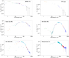 |
Fig. 1 Spectral energy distributions of the objects BRAN 76 (top left), EX Lupi (top right), Haro 5a IRS (middle left), HH 354 IRS (middle right), HH 381 IRS (bottom left), and Parsamian 21 (bottom right) including PACS spectra and photometry data (turquoise line + blue dots at 70, 100, and 160 μm), SPIRE high-resolution spectra (dark blue and red lines), and SPIRE photometry (black dots at 250, 350, and 500 μm) combined with spectra from Spitzer (lines in other colors below 50 μm) and photometry from other sources (diamonds; color-coded by source). |
BRAN 76
The PACS and SPIRE spectra have poor S/N, and are therefore not presented in the SED. The photometry in the SED closely matches the previous observations (Sandell & Weintraub 2001; Green et al. 2006; Reipurth et al. 2002; Skrutskie et al. 2006), closing the gap above Spitzer up to the sub-millimeter. The source resembles FU Ori, with silicate in emission (Fig. 3) and generally a weak far-infrared component, indicating that the source is not as embedded as the other FUors. Due to the higher robustness of the line fitting, as discussed above, we were able to measure a few CO transitions above a 3σ detection and obtained upper limits up to J = 38−37. We also find tentative evidence of water and OH lines (see Table B.1). Figure 9 shows diffuse emission around the object, mainly in the 160 μm channel, which traces cold dust, in the west and southeast. The SPIRE photometry shows mainly diffuse emission in the north, which does not appear to originate from the target.
EX Lup
EX Lupis the only EXor in our sample and the faintest object in our analysis (see Table 1 and Fig. 8). It is the prototype of its class and has shown several outbursts, in particular in 2008 during which its silicate, in emission, changed between quiescence and outburst, with evidence of thermal annealing in the surface layer of the inner disk by heat from the outburst (Ábrahám et al. 2009). The SED is shown in Fig. 1 with SPIRE and PACS photometry. We complement the SED with additional photometry (Helou & Walker 1988, Cutri et al. 2003) down to 12 micrometers, which match the PACS photometry in the intersecting area at 60 μm. There is no evidence of envelope emission, as previously inferred (e.g., Sipos et al. 2009). The Herschel photometry of EX Lup is point-like. We confirm the presence of LEDA 165 681 in the southeast, a background galaxy. The PACS line maps show centered emission on the target coordinates without any sort of outflows. We found only two CO lines with a 3σ detection at the target coordinates. In addition, these two lines show no significant emission in adjacent spaxels. We found emission above 3σ for other CO lines in the central 3 × 3 spaxels (see Appendix B), which provides further evidence that the CO detection is true. Additional data with higher sensitivity for CO are required for a deeper analysis of these lines, as we did for other objects with CO emission in this paper (see Fig. 5).
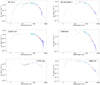 |
Fig. 2 Spectral energy distributions of the objects PP 13 S (top left), Re 50 N IRS 1 (also known as HBC 494) (top right), V1647 Ori (middle left), V346 Nor (middle right), V733 Cep (bottom left), and V883 Ori (bottom right). Data shown as in Fig. 1. The SED of faint objects (here V1647 Ori and V733 Cep) is complemented with low-resolution spectra from SPIRE (thick orange and purple lines at the same wavelength window as the high-resolution spectra). |
Haro 5a IRS
Published photometry (Skrutskie et al. 2006; Reipurth et al. 2004; Lis et al. 1998; Wolstencroft et al. 1986; Chini et al. 1997) complements the emission to the near-IR and millimeter range. PACS and SPIRE spectra in the SEDs show strong emission lines of atomic (OI) and molecular (CO) species, indicating high column densities. The wavelength of the SED peak emission lies slightly below 100 μm. In the images of PACS and SPIRE in Fig. 10, we can recognize more significant diffuse emission around the target with another object close by in the northeast (HOPS 85). There is also a filament, mainly in the 160 μm channel (red) in the north, which we can also find in the SPIRE data. The SPIRE data show also some stronger filament-like emission in the south, so that the target appears to be within a single filament. We detected CO lines from J = 4−3 to J = 10−9 in the SPIRE spectra, as well as 13CO J = 6−5 and J = 5−4. We detected two [C I] lines (370 and 609 μm) and provide an upper limit for [C I] at 230 μm. The emission in the SPIRE maps is for [C I] at 370 μm and the CO transmission from J = 9−8 to J = 5−4 separated in two areas. The first area is localized around the target coordinates, with a slight offset for [C I] to the northeast. The CO emission is more localized at the target coordinates, with higher emission in the southwest for CO J = 8−7. The second area is the southwest itself, which is emitting even more strongly than the source. Both areas correlate well with the RGB images of PACS and SPIRE, and are probably tracing the filament.
The Spitzer data show deep silicate absorption at 10 μm (stretching of the Si–O bonds), with a weaker component around 18 μm (O–Si–O bending), together with several ice features between 5 and 9 μm, due to H2O and HCOOH ice, CH3OH and NH , CH4, and NH3 at 8.5–9 μm (Fig. 3; see also Öberg et al. 2010 for identification of ice features). Furthermore, CO2 ice is detected at 15 μm (Fig. 4).
HH 354 IRS
The Herschel spectra completes the peak emission of the envelope in the SED, which was already partially detected in the Spitzer data. The SED, complemented by photometry below 10 μm (Skrutskie et al. 2006; Visser et al. 2002; Di Francesco et al. 2008; Kleinmann et al. 1986; Helou & Walker 1988), shows very deep absorption near the silicate feature (Fig. 3). The deep narrow absorption peak in the silicate feature can be identified as methanol ice (fundamental CO-stretch mode). CO2 ice is also detected at 15 μm (Fig. 4). In addition, the 5–9 μm also show ice features as detected in Haro 5a IRS.
While a companion is currently not known, there is a reflection nebula (Reipurth & Aspin 1997) surrounding the object, which likely contributes to some additional emission at lower wavelengths. HH 354 IRS appears to be isolated in the PACS images, with some slight diffuse emission in the northeast. This diffuse emission cannot be confirmed in the SPIRE data; however, there is some more emission in the north and the southeast. We see a very strong emission of [O I] at 63 μm and can detect [O I] at 145.5 μm. Both lines peak at the target coordinates, but the emission seems to also be affected by diffuse emission. We find OH, [N II] which is slightly enhanced at the source coordinates, several water lines, and CO transitions from J =5−4 to J =37−36, with an upper limit for the J = 38−37 transition. The SPIRE maps do not show a clear correlation with the RGB images. Some of the CO lines (J = 11−10, J =10−9) show emission distributed over a few spaxels, which are not always linked together, while other lines ([C I] at 370 μm, CO J = 7−6, [N II]) havemuch smoother emission, which is also extended over the entire field of view and which might indicate extended emission.
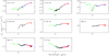 |
Fig. 3 Zoom-in of the Spitzer spectra for our targets (from the PI: Audard program). The colors of the different modules are black (SH), red (LH), green (SL), and blue (LL). The top three targets (and possibly HH 381 IRS) show evidence of H2O and HCOOH ice at ≈6 μm, CH3OH and NH |

Bolometric and 63 μm [O I] luminosities.
HH 381 IRS
Together with the Spitzer spectra and photometry between 1 and 3 μm, HH 381 IRS shows the SED of an embedded young stellar object, similar to Class I with strong continuum emission between 5 and 100 μm. Additional photometry (Skrutskie et al. 2006; Egan et al. 2003) from previous observations do not match the Herschel and Spitzer spectra closely, possibly due to significant variations in the mid- and far-infrared emission during the possible FUor outburst. This is further discussed in Sect. 4.2. The Spitzer data show weak silicate absorption at 10 μm (Fig. 3), much weaker than in other embedded FUors. Nevertheless, there is also a weak CO2 absorption detected in the IRS spectra (Fig. 4). Other ices < 10 μm are possibly detected as well.
Figure 11 shows HH 381 IRS as isolated with some weak emission in the south in the PACS data. SPIRE shows some more extended emission and a diffuse emission in the northeast and southwest around the target. 2MASS photometry from the J, H, and K bands shows bipolar outflows of the target, one in the north probably directed away from us, the other in the south probably directed toward the observer and with stronger intensity. The emission of OI is centered for the transition at 145.5 μm, but for 63 μm the maximum is in the neighboring spaxel southeast of the source. In addition to OI, the spectrum shows water lines: OH and CO from J = 7−6 to J = 37−36. 13CO is not detected, so we only provide upper limits. The emission of both [C I] lines and CO J = 7−6 is extended over a large area, while CO J = 8−7 is restricted mainly to the target coordinates and a small emission region in the southwest. That region matches the bump in the SPIRE RGB image in the southwest, where the OI emission at 145.5 μm also shows a signal.
Photometry flux densities of PACS and SPIRE for each wavelength window.
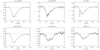 |
Fig. 4 Zoom-in of the Spitzer spectra for targets with CO2 ice absorption. Absorption optical depths τ near 15 μm were derived from F = F0e−τ, where F is the observed flux density, and F0 is the continuum derived from a continuum fit, obtained with a polynomial of degree N = 3 (red curve; HH 381 IRS, V883 Ori, BRAN 76, and V733 Cep needed N = 2) to fit the ranges 13.5–14.7 and 18.2–19.5 μm (except for HH 381 IRS and V883 Ori for which 13.5–14.7 and 16.0–17.0 μm were used). In addition, in some cases, a Gaussian function centered on 608 cm−1 (16.45 μm) and of FWHM = 73 cm−1 was added tofit the 16.5-18.2 μm range to account for absorption due to silicates. This method is similar to that used by Pontoppidan et al. (2008). Interestingly, we detect gas absorption by CO2 at 15.0 μm, but only in PP13 S. |
Parsamian 21
The available spectra of PACS and SPIRE are joined by photometry measurements (Helou & Walker 1988), which show the SED down to 10 μm. Parsamian 21 is affected by moderate noise in its spectrum, which makes it difficult to confirm lines above the 3σ threshold. The SED shows that the object is embedded, similar to YSO Class I, with a strong continuum from 10 to 100 μm. The Spitzerspectrum was shown by Kóspál et al. (2008) and shows strong CO2 absorption. Inversely to other FUors, it shows PAH features at 6.3, 8.2, and 11.3 μm and silicate emission at 10 μm. Kóspál et al. (2008) argued that Parsamian 21 was an intermediate-age FUor in the evolutionary sequence.
In our Herschel data, we find a few CO and OH lines in the data, but mostly provide upper limits. In the RGB images, Parsamian 21 appears isolated with some strong diffuse emission in the north in both PACS and SPIRE photometry. This outflow can also be seen in the optical (e.g., by DSS2 in the red (F+R) and blue (XJ+S) channel) and was first described by Parsamyan & Petrosyan (1978). In SPIRE, we can also recognize a second bump in the east of the northern end of the emission. We could not identify another source in that area, but as this emission is not visible in the PACS data, it simply might be material of lower temperature. The H2O emission in the PACS line maps shows an additional spaxel, which matches the outflow from the RGB images in the north.
PP 13 S
Together with external photometry (Sandell & Aspin 1998; Cohen et al. 1983; Osterloh & Beckwith 1995; Sandell & Weintraub 2001; Tapia et al. 1997) and the Spitzer spectra, the Herschel data completes the SED, ranging from 1 μm up to above 1 mm. The spectrum is characterized by strong continuum emission (≈ 10−10 erg s−1 cm−2) between 30 and 200 μm, indicative ofstrong envelope emission. The extinction is very high since the photometry drops significantly below 2 μm. Figure 3 shows very deep silicate absorption in the Si–O stretching feature at 10 μm and in the O–Si–O bending at 18 μm. In addition, CO2 ice absorption is detected, and interestingly a CO2 gas line is detected at 15.0 μm (Fig. 4). This is the only target showing such gas absorption feature in our sample. At shorter wavelengths (5−9 μm), the other ice features are detected as well, though NH3 ice appears weaker than in other targets.
PP 13S in Fig. 12 shows slight diffuse emission around the target in PACS data. However, we see some filamentary structures in the SPIRE data in the north of the target. There is also a stronger emission in the neighborhood around the target in the SPIRE data. We find emission lines in the spectra, namely the two OI lines at 63 and 145.5 μm, water, OH, [C I] and [C II], and CO from J = 4−3 to J = 37−36, and we provide upper limits for 13CO from J = 5−4 to J = 10−9. The PACS line maps show the emission of CO, H2O, and [O I] mostly centered around the object. Some CO lines are extended around the object, while in particular the H2O emission at 108 μm affects adjacent spaxels. The emission of [O I] at 63 μm shows an outflow in the north, possibly correlated with the filamentary structure in the SPIRE data. In the SPIRE maps, the emission is more extended, while there appears to be no clear link to the RGB images.
Re 50 N IRS 1/HBC 494
The SED fills the area from below 1 μm to above 1 mm, using published photometry (Reipurth et al. 1993; Dent et al. 1998; Zavagno et al. 1997; Sandell & Weintraub 2001; Strom et al. 1989; Helou & Walker 1988) in combination with Spitzer spectra. We find again strong continuum emission in the mid- and far-infrared, indicative of envelope emission. The Spitzer spectrum also shows deep silicate absorption (in both bending and stretching bands), although there is no spectrum available below 10 μm (Fig. 3). CO2 absorption is also detected (Fig. 4), although without a gas absorption line, in spite of the relatively similar SED as PP 13 S. The source appears to have rebrightened between 2006 and 2014 (Chiang et al. (2015); the Spitzer data were taken 7 Nov 2008, while the Herschel date from Sep 2013). The source is known to harbor a very wide outflow, detected with ALMA (Ruíz-Rodríguez et al. 2017b).
In the RGB images, Re 50 N IRS 1 shows strong diffuse emission in an extended area in both the PACS and the SPIRE data. The PACS data extend mostly in the northeast and also in the west of the object, while SPIRE shows some weaker diffuse emission in the west, but confirms the emission in the northeast. We can also see a second emission bump in the south of theobject with both instruments. Unfortunately, the Spitzer data for Re 50 N IRS 1 stop short of 10 μm. In the Herschel spectra, we see water lines, both O I lines, several OH lines, [C I] and [C II], and CO lines from J =4−3 to J =37−36 transition. We can also detect [N II] at 205 μm. The line maps of PACS are centered around the target coordinates, while the SPIRE maps show a bigger emission of the surrounding area. There appears to be no correlation to the shape of the object in the RGB images. However, especially the [C I] line at 370 μm and the CO J = 7 −6 emission peaks clearly at the center, which indicates that the emission is not in the foreground but originates from the object.
V346 Nor
The corresponding spectrum of Herschel has been complemented by photometric measurements (Helou & Walker 1988; Kenyon & Hartmann 1991; Kóspál et al. 2017; observed 2013.5) down to 2 μm, covering the peak emission of the object. Spitzer data (Green et al. 2006; not shown in this paper) reveal deep silicate absorption at 10 μm, a CO2 ice absorption feature, together with the other ice features in the 5−9μm range. Following the light curve of Kóspál et al. 2017, our Herschel data (February–March 2013) were observed during the re-brightening phase of V346 Nor, which followed a fade with minimum in 2010.
The SPIRE data of V346 Nor in Fig. 13 shows extended diffuse emission around the target in the west, east, and north. The PACS data reveal multiple individual sources: a strong one in the west, which we identify as 2MASS 16322723-4455303 and 2MASS 16322723-4455314; a strong (2MASS 16323031-4455189) and a faint source (2MASS 16323337-4455187) in the north; and a very faint source in the east (2MASS 16323553-4455317) of V346 Nor. In the spectrum of PACS and SPIRE we can easily recognize several emission lines. Our fitting found water lines, both OI lines, [N II], [C I] and [C II], and CO lines from J = 4−3 to J = 37−36, in addition to 13CO lines between J = 5−4 and J = 8−7. Emission in the linemaps of PACS is mainly concentrated around the target with some spaxels, mostly of lower transitions, showing emission in the vicinity. The continuum-subtracted maps of SPIRE show a slightly extended emission, similar to the extended emission of the photometry in the RGB image of SPIRE. The [C I] emission at 370 μm in contrast to the emission at 609 μm shows at least an emission peak at the coordinates of the target, so foreground or background emission can be excluded here. The CO J = 11−10 and J = 9−8 transition represents very well what can be seen in the RGB image, while others (J = 4−3 to J = 7−6) show more extended emission over a large area. Even though the diffuse emission of [N II] is extended over the entire field of view, the emission peak at the coordinates of the source, which is up to an order of magnitude higher, makes it likely that V346 Nor is the origin of the emission here. The contribution of other nearby objects cannot be eliminated, however.
V733 Cep
Due to the poor quality, we do not show the spectrum of PACS, and only provide the low-resolution spectrum of SPIRE. The data are combined with spectra from Spitzer in the mid-IR and with photometry (Semkov & Peneva 2008; Skrutskie et al. 2006; Egan et al. 2003) down to slightly above 400 nm. The shape of the SED is peculiar compared to the other targets, as it shows significant emission below 10 μm likely due to the central source and disk emission, while there is an additional component in the far-infrared regime, likely a remainder of an envelope, possibly indicating that V733 Cep is of intermediate age in the evolutionary sequence proposed for FUors, i.e., between Class I and II YSO. The Spitzer data do not show a clear silicate feature, or possibly a very weak absorption feature, with also very weak ice features below 10 μm. There is, however, no evidence of CO2 ice absorption at 15 μm (Fig. 3).
V733 Cep shows in PACS data bright emission around the source coordinates, with another object in the southwest and a cluster of objects in the southeast of the target. In the SPIRE data, we cannot resolve individual objects of this cluster; however, the emission of V733 is dominated by the blue (250 μm) emission, while the other bands do not outshine the background. We identified in the data O I at 145.5 μm, [N II], [C I], and [C II], and some CO lines ranging from J = 4−3 to J = 33−32. The SPIRE line maps show the strongest emission for most lines in the southeast of the target, where we find the already mentioned cluster. We therefore do not assume that the (main) emission originates from V733 Cep, but from the objects nearby. For the [N II] emission, again we cannot tell if this is foreground or originating from the observed area.
CO rotational temperatures and column densities.
V883 Ori
The SED of V883 Ori is shown with Spitzer and Herschel spectra, and complemented by published photometry (Reipurth et al. 1993; Dent et al. 1998; Molinari et al. 1993; Sandell & Weintraub 2001; Cutri et al. 2003; Egan et al. 2003) ranging from the visible to above 1 mm. The SED is flat from 3 μm to about 60 μm. The Spitzer spectrum shows weak silicate absorption (though again cut below 10 μm) and weak CO2 ice absorption (Figs. 3 and 4).
For V883 Ori in Fig. 14, we find diffuse emission in the PACS data in the north of the target, forming a bar from the east to the northwest of the target. The emission overlaps in the east with the position of several 2MASS objects (2MASS 05382028-0702353, 2MASS 05381975-0702261, 2MASS 05381936-0702241, 2MASS 05381922-0702287, and 2MASS 05381868-0702241). It is uncertain how much of the diffuse emission is contributed by the 2MASS objects and how much originates from V883 Ori. We do not find another object in the emission in the north, so at least that component likely originates from our target. The SPIRE data appear dominated by V883 Ori, which causes some artifacts in all three bands, with some strong diffuse emission in the northwest, for which we also do not find a known object. The object shows [O I] and some OH lines, as well as [N II], [C II], and [C I]. We report the detection of CO from J = 4−3 to J = 33−32 transition. The [C I] lines in the SPIRE maps smoothly peak at the target coordinates, with diffuse emission around it. The CO and [N II] lines do not show such a clear picture.
V1647 Ori
V1647 Ori, an object intermediate between FUors and EXors, is shown together with photometry (Reipurth & Aspin 2004; Aspin 2011; Mosoni et al. 2013) in the IR. The object has shown significant flux variations since its initial outburst in 2003 and was observed on many occasions from the optical to the millimeter ranges, decaying in 2006 and outbursting again in 2008 (see Aspin et al. 2009 and Audard et al. 2014 and references therein).
The SPIRE spectra are quite noisy; therefore, we also provide the low-resolution spectra, even though they do not resolve any lines. In the images, we find diffuse emission around the target, especially in the PACS data. We identify emission knots in the north (HH 22 MIR), which also shows significant diffuse emission in the SPIRE data, and the southwest (2MASS J05461162-0006279), which does not separate from the background emission in SPIRE. There is also some faint extension of diffuse emission from V1647 Ori in PACS, going westward, which increases at some distance in the SPIRE data. The spectra show both [O I] transitions, OH, [N II], and [C I] and CO transitions from J =4−3 to J =25−24. For the higher lines up to J = 37−36 and for most 13CO lines we provide upper limits. The emission of [C I] at 370 μm, and the CO J = 7−6 and J = 6−5 lines show the strongest emission off-source in the northeast where the object HH 22 MIR can be seen in the RGB images. It is not clear how much of the emission is contributed by V1647 Ori. The [N II] emission behaves differently, showing less diffuse emission than most other objects, with a peak at the target coordinates, indicating that that emission originates from the source.
4.2 SED variability
We found differences in the SEDs (Figs. 1 and 2) between our data and earlier observations for HH 381 IRS (8.28–100 μm) and PP 13 S (50–160 μm). The numerical factors were obtained by measuring the difference in the photometry to the spectrum of Herschel and Spitzer at the same wavelength. In the case of PP 13 S, the offset is up to factor 1.7 (Cohen et al. 1983) (observed 1981), while the measurements of the InfraRed Astronomical Satellite (IRAS, observed 1983.5) and Herschel (PACS photometry: March 2013) in the PACS range match. For HH 381 IRS, the offset ranges between a factor of 8.5 and 43.8 for the Midcourse Space Experiment (MSX; data observed in 1996–1997) and 1.8–2.7 for IRAS (1983.5), compared to the Herschel photometry (PACS photometry: November 2012).
As there are already strong differences in the published data (at least for HH 381 IRS), and since the observations of Spitzer (2010) and Herschel match quite well, it is unlikely that there is an issue with the observation. We therefore assume that the objects increased their luminosities over time, which took place in the IR.
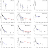 |
Fig. 5 CO rotational diagrams of all objects. We plot the decadic logarithm of the column densities Nu divided by the statistical weight gu, as function of the upper level energy of the transition Eu in Kelvin. SPIRE data are fitted with black, PACS data are fitted with blue and red. As the plots contain a logarithmic scale, the errors are actually not symmetric, but we use it here as an approximation. |
4.3 Rotational diagrams
We derived CO rotational temperature for our targets; they can be found in Table 3, where the column density is also listed. The method that we used is described in Goldsmith & Langer (1999) in detail and was applied on Herschel data in Green et al. (2013b) and Dionatos et al. (2013). We used the same approach as Green et al. (2013b), separating the data into three domains of LTE, one for SPIRE (Jup ≤ 13 or Eu ≤ 505 K) and two for the different PACS orders (PACS R1, in this paper called PACS long for 14 ≤ Jup ≤ 24 or 560 K ≤ Eu ≤ 1670 K, and PACS B2A/B2B, in this paper called PACS short for Jup ≥ 25 or Eu > 1700 K). However, we use the luminosity L of the CO lines instead of the fluxes (same approach as in Dionatos et al. 2013) to eventually obtain the column densities log10(N) of the molecules. Data for the upper level energy Eu, Einstein coefficients Aul, and partition function Q were obtained by the Cologne Database for Molecular Spectroscope (CDMS; Müller et al. 2005). For the plots, Nu is given by L × 4π∕(h × νul × Aul), which is divided by the statistical weights of the respective line. As a function of the upper energy level Eu, a line can be fitted in which the slope m measures the rotation temperature via Trot = −1∕(m ×log(10)). The height of the line h can be further used to calculate the column density of the data by following log10(N) = h + log10(Q). We mention here that the rotation temperatureTrot of the CO does not necessarily represent the kinetic temperature Tkin of the gas. Figure 5 shows the individual fits to the CO rotation data to derive the CO rotational temperatures and column densities. Due to the small number of lines in some ranges, we also used CO lines below the 3σ limit. However, the fitting routine takes into account the error and uses a weighting so that lines with a large error do not have a too strong impact on the fitting result. Lines below the 3σ limit are accordingly marked in the tables (see Table B.1). We tried to find a correlation between the different rotational temperatures. The cold temperature from the SPIRE data and the warmer temperature from the PACS long data, shown in Fig. 7, provided enough data points for an analysis. Based on the available data, we could not find a correlation or conspicuousness among the objects. Figure 6 shows a histogram of the CO rotational temperature of our targets, and complements it with values derived for other classical FUors, V1057 Cyg, V1331 Cyg, V1515 Cyg, and V1735 Cyg, as derived by Green et al. (2013a). We also found in our sample several low-temperature components on the order of 0−100 K; however, many targets in our sample have temperatures around 400−500 K, and possibly very hot temperature components of 1000−1500 K. This will be discussed in more detail in the next section.
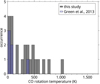 |
Fig. 6 Occurrence of the CO rotation temperatures found in our targets and for V1057 Cyg, V1331 Cyg, and V1515 Cyg from Green et al. (2013a). Temperatures above 1700 K are not shown here because of the high uncertainty of the measurements. |
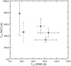 |
Fig. 7 Temperature measurements of PACS long as a function of SPIRE measurements. Only temperatures derived by at least three CO lines are shown (see Table 3) in order to have more robust error bars. |
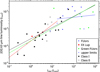 |
Fig. 8 [O I] luminosity at 63 μm as a function of the bolometric luminosity of the object. The black curve represents the best-fit result of the data with f(x) = 0.65 ⋅ x − 3.6 and χ2 = 7.8. We show two additional lines which partially fit the data (in red) with f(x) = 0.94 ⋅ x −3.7, Lbol <17 L⊙, and χ2 = 3.5, and (in blue)with f(x) = 0.13 ⋅ x − 2.6, Lbol >17 L⊙, and χ2 = 3.2. We also show the best fit of Green et al. (2013a) with f(x) = 0.70 ⋅ x − 3.7 (in green). The data points that are indicated as upper limits (3σ) and EX Lup are not used to create the fits. |
5 Discussion
5.1 CO temperature components
Several objects show low-J transitions of CO in the SPIRE range, revealing a cool component (< 100 K). The rotational diagram indicates temperatures on the order of 40−50 K, with a few objects showing lower temperatures, such as V883 Ori, and V1647 Ori, and high column densities. No evidence of low temperatures is found in Parsamian 21, with no detected lines in the SPIRE range above 3σ.
For the CO rotational lines in the PACS long range, the uncertainties on the temperature do not allow us to distinguish differences in the targets. This range consistently provides values on the order of 400 K (Parsamian 21, V883 Ori, and HH 381 IRS show higher temperatures, but large uncertainties due to the low number of lines available). Interestingly, even when low-J transitions were not detected (i.e., no low rotational temperature) CO emission lines showing a “medium” temperature was almost always found, suggesting that this component is ubiquitous in outbursting young sources.
The PACS short range, where high-J transitions lie, has revealed very few detected lines, making the detection of a hot component (> 1000 K) difficult to assess. There is a suggested presence of such a component in HH 381 IRS and HH 354 IRS, albeit with large uncertainties. V883 Ori, on the other hand, shows a temperature similar to that in the PACS long range, suggesting that the hot component does not exist in this target; it is interesting to note that this same target also shows the coolest temperature in SPIRE, suggesting that V883 Ori generally has a lower temperature than other targets. V346 Nor may display a hot component, again with a rather large uncertainty.
The similarity of the line fluxes in those objects compared to HH 381 IRS, but the strong difference in the high-temperature domain, might be related to the luminosity increase of HH 381 IRS (further discussed in Sect. 5.3), although we caution that few lines were detected, probably because of the higher noise and stronger continuum. Optical depth effects (e.g., due to the optical thickness of the dust continuum) may play a role, although the SEDs (dominated by dust emission) are similar to other targets with weak or no CO emission in the PACS range, as discussed above.
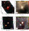 |
Fig. 9 Three-color composed image of the 70 μm (blue), 100 μm (green), and 160 μm (red) photometry of PACS (left) and 250 μm (blue), 350 μm (green), and 500 μm (red) photometry of SPIRE (right) for Bran 76 (top) and EX Lup (bottom). The target coordinates of the FUor/EXor are shown with a blue cross. The circle in the lower left corner represents the beam for the longest used wavelength of the respective image (11.5″ for PACS, 35.95″ for SPIRE). For the PACS images we used an asinh scaling with 99.5% cutoff but removed values below zero. For SPIRE, we used a linear scale with 99.5% cutoff. |
5.2 Evolved objects
For the more evolved objects in our sample, EX Lup (with no envelope) or BRAN 76 (a possibly evolved FUor with less envelope and a silicate feature in emission, like FU Ori), our spectra are quite noisy. Our analysis has tentatively detected a few CO lines in EX Lup (see Sect. 4.1), despite the formal statistical uncertainties. BRAN 76, on the other hand, displayed CO emission only in the PACS short range. V1647 Ori, whose classification is unclear and with its flat SED, shows enough signal for the detection of several CO lines. For the moment there is not enough evidence to make a link between the detectability of molecular or atomic lines and the properties of the targets. In a subsequent analysis, we will investigate this issue by modeling the objects with the radiation thermo-chemical code ProDiMo (Woitke et al. 2009), and thus derive geometrical information on the emission lines, in particular thanks to the enhanced version of the code by Rab et al. (2017) that takes into account the envelope around outbursting sources.
5.3 Young embedded objects
Our sample of outbursting sources shows a large variety of SEDs. Quanz et al. (2007) suggested that this could be due to the evolutionary stage (Class I versus Class II YSO), but some features cannot be explained by the evolutionary stage alone. PP 13 S, V883 Ori, HH 381 IRS, and V346 Nor, which are all FUors or FUor-like objects, show similar shapes of their SEDs and should in the Quanz scheme be in a similar evolutionary stage. Therefore, the question arises whether there is any correlation between properties among those objects. For the emission lines in these targets, they are strongest in PP 13 S and V346 Nor, while V883 Ori and HH 381 IRS show lines on a much lower level in the SEDs, despite similar continuum levels in the far-infrared. The lines themselves are very different between PP 13 S and V346 Nor. While PP 13 S shows strong atomic oxygen emission and only moderate CO, V346 Nor shows strong CO emission but weak oxygen. The CO2 gas absorption at 15μm is unique among our targets, and even compared to other YSOs it appears very rarely, both in absorption and emission (Lahuis et al. 2005; Poglitsch et al. 2010). For HH 381 IRS we note the increased luminosity over the last years in the IR. A strong increase in luminosity on a long timescale indicates that it might be at the beginning phase of a long outburst, with a strong mass accretion onto the embedded object. However, we note that, although detected, the [O I] line flux at 63 μm, a common tracer of high accretion rates (Green et al. 2013a), is particularly weak in HH 381 IRS, like the other detection of OH, H2O, and CO lines. Taking into account the distance and looking at the luminosity of the line (see Fig. 8), the [O I] emission of HH381 appears to be among the more luminous objects in our sample, still below V346 Nor and about one order of magnitude above PP 13 S. For HH 381 IRS, the controversy between the rising bolometric luminosity and the absence of strong accretion tracers is very interesting as it shows that the bolometric luminosity is not dominated by accretion luminosity, but instead is dominated by photospheric luminosity of the central source. The mass accretion and accretion luminosity may quickly drop after the onset of the burst because of the exhausted mass reservoir in the innermost disk, but the star bloats in response to the accreted energy which leads to a dramatic increase in the photospheric luminosity. As a result the total luminosity may keep rising. Similar situations in the evolution of bursting stars were shown recently in Elbakyan et al. (2019). As we did for the evolved objects, we will investigate the characteristics of the young objects in the future with ProDiMo since for the moment there is no correlation visible.
5.4 Correlation between lines
In the following, we discuss the correlation between lines that have been found either in our data or by other groups, in which case we check their consistency within our sample of YSOs. In Fig. 8 we show the luminosity of the [O I] emission at 63 μm as a function of the bolometric luminosity of our targets in a log-log plot. Table 1 shows the 63 μm [O I] luminosity of our targets. Haro 5a IRS is missing here. For Parsamian 21, V733 Cep, and V883 Ori we only show upper limits. In addition to our sample, we used HBC 722, V1735 Cyg, V1057 Cyg, V1515 Cyg, and FU Ori from Green et al. (2013a). Along with the targets, we show our best-fit result as black line in the plot (not including the upper limits and EX Lup). We find a clear correlation of the bolometric luminosity and the luminosity of the 63 μm emission line with f(x) = 0.65 ⋅ x − 3.6. However, as mentioned in Sect. 5.3, some objects do not follow this principle. Due to the “knee” at ≈17 L⊙, we created two other fits, one for L > 17 L⊙ and one for L < 17 L⊙. For comparison, the analysis of Green et al. (2013a) resulted in f(x) = 0.70 ⋅ x − 3.7. Our sample of FUors is still small, but it seems that FUors experience a saturation of [O I] emission compared to Class 0/I objects. However, this behavior is mainly caused by four of the targets from Green et al. (2013a) and needs further investigation.
Remarkably, our analysis suggests the tentative detection of multiple water and OH emission lines in the PACS data for PP 13 S, Re 50 N IRS 1, and V346 Nor, and possibly other targets, where we see the water emission in a slightly extended area around each target. We did not find a correlation between the presence of water and OH, but we will investigate this possibility during our upcoming analysis when taking into account spatial properties.
Among the DIGIT and HOPS objects, Green et al. (2013a) find that a strong CO J = 16−15 line correlates well with N(PACS long). We find the strongest emission of this particular CO line in PP 13 S, Re 50 N IRS 1, and V346 Nor, each with very strong emission lines in general. These objects show the highest column densities in the PACS data at warm temperature (PACS long) among our sample, clearly supporting this result.
Furthermore, Green also discussed the possibility that Class 0/I objects (FUors and FUor-like) have hotter and more excited CO rotation lines than Class II objects. The most Class II-like objects in our sample are EX Lupi (EXor) and V1647 Ori (likely EXor). Both objects show, if our data allows an analysis, relatively low temperatures compared to the rest of our sample, which supports this assumption.
Green et al. (2013a) argued that weak silicate features, in emission or absorption, do not correlate well with [O I] emission. In our sample, the Spitzer data show strong silicate features for Haro 5a IRS, PP 13 S, and Re 50 N IRS 1. HH 354 IRS also shows strong absorption near the silicate feature, although in that case the strong absorption is also due to water ice. The targets show severalother ice features, such as water, methanol and ammonium, methane, and ammonia and carbon dioxide at 15 μm (Figs. 3 and 4). We note that a CO2 gas line was detected in absorption in PP13 S, the only target in our sample showing this feature. Each of these targets shows strong emission of [O I] at 63.1μm and emission of the 145.5 μm line above the 3σ limit. In addition, V883 Ori and HH 381 IRS, weak [O I] emitters, show weak silicate absorption. HH 381 IRS, the only target for which Spitzer covered the 5–10 μm range as well, also did not detect evidence of the other ice components. It provides further evidence that the correlation suggested by Green et al. (2013a) is indeed strong.
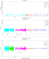 |
Fig. 15 Continuum-subtracted spectra of PACS and SPIRE for Haro 5a IRS, HH 354 IRS, and HH 381 IRS. For the indicators of the lines, we use a 1.5−σ lower limit. |
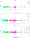 |
Fig. 16 Continuum-subtracted spectra of PACS and SPIRE for PP 13S, Re 50 N IRS/HBC 494, and V346 Nor. |
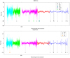 |
Fig. 17 Continuum-subtracted Spectra of PACS and SPIRE for V883 Ori and V1647 Ori. |
6 Summary
We provided the SEDs, including photometry and integral field spectroscopy of 12 FUors and EXors using mainly Herschel and Spitzer data, and additional published photometry. In most cases we covered the SED from the optical or near-IR up to the sub-millimeter range, tracing the emission of the envelope and disk of the targets. Our observationsrevealed the complex environment in which most of our targets reside, which we discuss in detail. The targets show a wide variety of spectral features, from silicate in absorption to emission, and often ice features from CO2 and other molecules from 5−9 μm, when embedded. We detected for one of our targets a rare CO2 gas absorption at 15 μm. We derived CO rotation temperatures in three temperature domains, finding different temperature regimes: < 100 K and 400−500 K. A third high-temperature component may be present in some targets as well. We provided three-color images of the targets in the PACS and SPIRE wavelength ranges. Finally, we provided line maps and line fluxes. We tentatively detected water emission for PP 13 S, Re 50 N IRS 1, and V346 Nor. We found a significant increase of luminosity in HH 381 IRS and PP 13 S, possibly due to early phases of an outburst. With our data set, we aim to use the data of all the objects in our sample for further analysis with ProDiMo to refine the models of outbursting sources and derive properties of the targets, namely the circumstellar disk and the surrounding envelope.
Acknowledgements
We thank the Swiss National Science Foundation (SNSF) (project number 200021L_163172) and the Austrian Science Fund (FWF) (project number I2549-N27) for their funding of this project. M.A. thanks C. Pearson for his early reduction of the SPIRE data. We thank A. Kospal for providing the Spitzer IRS spectrum for Parsamian 21. O. Dionatos acknowledges support from the Austrian Research Promotion Agency (FFG) under the framework of the Austrian Space Applications Program (ASAP) projects JetPro* and PROTEUS (FFG-854025, FFG-866005). This publication makes use of data products from the Two Micron All Sky Survey, which is a joint project of the University of Massachusetts and the Infrared Processing and Analysis Center/California Institute of Technology, funded by the National Aeronautics and Space Administration and the National Science Foundation.
Appendix A PACS/SPIRE line maps
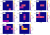 |
Fig. A.1 Line maps of PACS with visible lines for HH354 IRS. The maps show a specific bandwidth around emission lines of molecularor atomic transitions in the spectra coming from the integral field spectroscopy from PACS. The bandwidth is defined for each source by a fitting routine. A threshold cuts off noise below a specific value. For molecular lines, the species is mentioned in the upper left corner of the plot, together with the energy transition for CO and its isotopolog and the wavelength for other molecules. For the atomic lines, next to the isotope we give the frequency of the transition. The circle in each of the plots represents the coordinates of the optical FUor/EXor. |
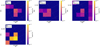 |
Fig. A.2 Line maps of PACS with visible lines for HH 381 IRS. |
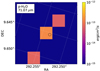 |
Fig. A.3 Line maps of PACS with visible lines for Parsamian 21. |
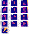 |
Fig. A.4 Line maps of PACS with visible lines for PP 13 S. |
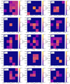 |
Fig. A.5 Line maps of PACS with visible lines for Re 50 N IRS 1, part 1. |
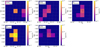 |
Fig. A.6 Line maps of PACS with visible lines for Re 50 N IRS 1, part 2. |
 |
Fig. A.7 Line maps of PACS with visible lines for V1647 Ori. |
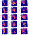 |
Fig. A.8 Line maps of PACS with visible lines for V346 Nor, part 1. |
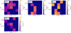 |
Fig. A.9 Line maps of PACS with visible lines for V346 Nor, part 2. |
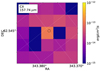 |
Fig. A.10 Line maps of PACS with visible lines for V733 Cep. |
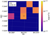 |
Fig. A.11 Line maps of PACS with visible lines for V883 Ori. |
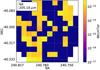 |
Fig. A.12 Line maps of SPIRE with visible lines for EX Lup. |
 |
Fig. A.13 Line maps of SPIRE with visible lines for Haro 5a IRS. |
 |
Fig. A.14 Line maps of SPIRE with visible lines for HH 354 IRS. |
 |
Fig. A.15 Line maps of SPIRE with visible lines for HH 381 IRS. |
 |
Fig. A.16 Line maps of SPIRE with visible lines for Parsamian 21. |
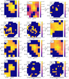 |
Fig. A.17 Line maps of SPIRE with visible lines for PP 13 S. |
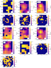 |
Fig. A.18 Line maps of SPIRE with visible lines for Re 50 N IRS 1. |
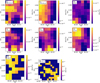 |
Fig. A.19 Line maps of SPIRE with visible lines for V1647 Ori. |
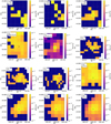 |
Fig. A.20 Line maps of SPIRE with visible lines for V346 Nor, part 1. |
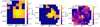 |
Fig. A.21 Line maps of SPIRE with visible lines for V346 Nor, part 2. |
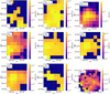 |
Fig. A.22 Line maps of SPIRE with visible lines for V733 Cep. |
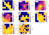 |
Fig. A.23 Line maps of SPIRE with visible lines for V883 Ori. |
References
- Ábrahám, P., Juhász, A., Dullemond, C. P., et al. 2009, Nature, 459, 224 [NASA ADS] [CrossRef] [PubMed] [Google Scholar]
- Aspin, C. 2011, AJ, 142, 135 [NASA ADS] [CrossRef] [Google Scholar]
- Aspin, C., Reipurth, B., Beck, T. L., et al. 2009, ApJ, 692, L67 [NASA ADS] [CrossRef] [Google Scholar]
- Audard, M., Ábrahám, P., Dunham, M. M., et al. 2014, Protostars and Planets VI (Tucson: University of Arizona Press), 387 [Google Scholar]
- Chiang, H.-F., Reipurth, B., Walawender, J., et al. 2015, ApJ, 805, 54 [NASA ADS] [CrossRef] [Google Scholar]
- Chini, R., Reipurth, B., Ward-Thompson, D., et al. 1997, ApJ, 474, L135 [NASA ADS] [CrossRef] [Google Scholar]
- Cieza, L. A., Casassus, S., Tobin, J., et al. 2016, Nature, 535, 258 [NASA ADS] [CrossRef] [Google Scholar]
- Cohen, M., Aitken, D. K., Roche, P. F., & Williams, P. M. 1983, ApJ, 273, 624 [NASA ADS] [CrossRef] [Google Scholar]
- Cutri, R. M., Skrutskie, M. F., van Dyk, S., et al. 2003, VizieR Online Data Catalog: II/246 [Google Scholar]
- de Graauw, T., Helmich, F. P., Phillips, T. G., et al. 2010, A&A, 518, L6 [NASA ADS] [CrossRef] [EDP Sciences] [Google Scholar]
- Dent, W. R. F., Matthews, H. E., & Ward-Thompson, D. 1998, MNRAS, 301, 1049 [NASA ADS] [CrossRef] [Google Scholar]
- De Wit, W.-J., Caratti, A., & Kraus, S. 2017, in Star Formation from Cores to Clusters (Vitacura, Santiago: ESO Workshop), 15 [Google Scholar]
- Di Francesco, J., Johnstone, D., Kirk, H., MacKenzie, T., & Ledwosinska, E. 2008, ApJS, 175, 277 [NASA ADS] [CrossRef] [Google Scholar]
- Dionatos, O., Jørgensen, J. K., Green, J. D., et al. 2013, A&A, 558, A88 [NASA ADS] [CrossRef] [EDP Sciences] [Google Scholar]
- Egan, M. P., Price, S. D., Kraemer, K. E., et al. 2003, VizieR Online Data Catalog: V/114 [Google Scholar]
- Elbakyan, V. G., Vorobyov, E. I., Rab, C., et al. 2019, MNRAS, 484, 146 [NASA ADS] [CrossRef] [Google Scholar]
- Fischer, W. J., Megeath, S. T., Tobin, J. J., et al. 2012, ApJ, 756, 99 [NASA ADS] [CrossRef] [Google Scholar]
- Fischer, W. J., Megeath, S. T., Stutz, A. M., et al. 2013, Astron. Nachr., 334, 53 [NASA ADS] [CrossRef] [Google Scholar]
- Goldsmith, P. F., & Langer, W. D. 1999, ApJ, 517, 209 [NASA ADS] [CrossRef] [Google Scholar]
- Green, J. D., Hartmann, L., Calvet, N., et al. 2006, ApJ, 648, 1099 [NASA ADS] [CrossRef] [Google Scholar]
- Green, J. D., Evans, II, N. J., Kóspál, Á., et al. 2013a, ApJ, 772, 117 [NASA ADS] [CrossRef] [Google Scholar]
- Green, J. D., Evans, II, N. J., Jørgensen, J. K., et al. 2013b, ApJ, 770, 123 [NASA ADS] [CrossRef] [Google Scholar]
- Griffin, M. J., Abergel, A., Abreu, A., et al. 2010, A&A, 518, L3 [Google Scholar]
- Hartmann, L., & Kenyon, S. J. 1996, ARA&A, 34, 207 [NASA ADS] [CrossRef] [EDP Sciences] [MathSciNet] [Google Scholar]
- Helou, G., & Walker, D. W., eds. 1988, Infrared Astronomical Satellite (IRAS) Catalogs and Atlases: The Small Scale Structure Catalog (Pasadena: Jet Propulsion Laboratory), 7, 1 [Google Scholar]
- Herbig, G. H. 1989, ESO Conf. Workshop Proc., 33, 233 [Google Scholar]
- Higdon, S. J. U., Devost, D., Higdon, J. L., et al. 2004, PASP, 116, 975 [NASA ADS] [CrossRef] [Google Scholar]
- Kenyon, S. J., & Hartmann, L. W. 1991, ApJ, 383, 664 [NASA ADS] [CrossRef] [Google Scholar]
- Kenyon, S. J., Kolotilov, E. A., Ibragimov, M. A., & Mattei, J. A. 2000, ApJ, 531, 1028 [NASA ADS] [CrossRef] [Google Scholar]
- Kleinmann, S.G., Cutri, R. M., Young, E. T., Low, F. J., & Gillett, F. C. 1986, IRAS Serendipitous Survey Catalog (Tucson: University of Arizona) [Google Scholar]
- Kóspál, Á., Ábrahám, P., Apai, D., et al. 2008, MNRAS, 383, 1015 [NASA ADS] [CrossRef] [Google Scholar]
- Kóspál, Á., Ábrahám, P., Westhues, C., & Haas, M. 2017, A&A, 597, L10 [NASA ADS] [CrossRef] [EDP Sciences] [Google Scholar]
- Lahuis, F., van Dishoeck, E. F., Boogert, A. C. A., et al. 2005, ApJ, 636, L145 [Google Scholar]
- Lebouteiller, V., Bernard-Salas, J., Sloan, G. C., & Barry, D. J. 2010, PASP, 122, 231 [NASA ADS] [CrossRef] [Google Scholar]
- Lis, D. C., Serabyn, E., Keene, J., et al. 1998, ApJ, 509, 299 [Google Scholar]
- Liu, H. B., Vorobyov, E. I., Dong, R., et al. 2017, A&A, 602, A19 [NASA ADS] [CrossRef] [EDP Sciences] [Google Scholar]
- Lorenzetti, D. 2005, Space Sci. Rev., 119, 181 [NASA ADS] [CrossRef] [Google Scholar]
- Meyer, D. M.-A., Vorobyov, E. I., Kuiper, R., & Kley, W. 2017, in Proceedings of the 3rd bwHPC-Symposium, Heidelberg 2016, eds. S. Richling, M. Baumann, & V. Heuveline (Heidelberg: Deutsche Nationalbibliothek) [Google Scholar]
- Molinari, S., Liseau, R., & Lorenzetti, D. 1993, A&AS, 101, 59 [NASA ADS] [Google Scholar]
- Mosoni, L., Sipos, N., Ábrahám, P., et al. 2013, A&A, 552, A62 [NASA ADS] [CrossRef] [EDP Sciences] [Google Scholar]
- Müller, H. S. P., Schlöder, F., Stutzki, J., & Winnewisser, G. 2005, J. Mol. Struct., 742, 215 [NASA ADS] [CrossRef] [Google Scholar]
- Öberg, K. I., Bottinelli, S., Jørgensen, J. K., & van Dishoeck, E. F. 2010, ApJ, 716, 825 [NASA ADS] [CrossRef] [Google Scholar]
- Osterloh, M., & Beckwith, S. V. W. 1995, ApJ, 439, 288 [NASA ADS] [CrossRef] [Google Scholar]
- Ott, S. 2010, ASP Conf. Se., 434, 139 [Google Scholar]
- Parsamyan, É. S., & Petrosyan, V. M. 1978, Astrophysics, 14, 289 [NASA ADS] [CrossRef] [Google Scholar]
- Pérez, L. M., Carpenter, J. M., Andrews, S. M., et al. 2016, Science, 353, 1519 [NASA ADS] [CrossRef] [Google Scholar]
- Pilbratt, G. L., Riedinger, J. R., Passvogel, T., et al. 2010, A&A, 518, L1 [CrossRef] [EDP Sciences] [Google Scholar]
- Poglitsch, A., Waelkens, C., Geis, N., et al. 2010, A&A, 518, L2 [NASA ADS] [CrossRef] [EDP Sciences] [Google Scholar]
- Pontoppidan, K. M., Boogert, A. C. A., Fraser, H. J., et al. 2008, ApJ, 678, 1005 [NASA ADS] [CrossRef] [Google Scholar]
- Quanz, S. P., Henning, T., Bouwman, J., Linz, H., & Lahuis, F. 2007, ApJ, 658, 487 [NASA ADS] [CrossRef] [Google Scholar]
- Rab, C., Elbakyan, V., Vorobyov, E., et al. 2017, A&A, 604, A15 [NASA ADS] [CrossRef] [EDP Sciences] [Google Scholar]
- Reipurth, B., & Aspin, C. 1997, AJ, 114, 2700 [NASA ADS] [CrossRef] [Google Scholar]
- Reipurth, B., & Aspin, C. 2004, ApJ, 606, L119 [NASA ADS] [CrossRef] [Google Scholar]
- Reipurth, B., & Aspin, C. 2010, in Evolution of Cosmic Objects through their Physical Activity, eds. H. A. Harutyunian, A. M. Mickaelian, & Y. Terzian (Armenia: National Academy of Sciences of the Republic of Armenia), 19 [Google Scholar]
- Reipurth, B., Chini, R., Krugel, E., Kreysa, E., & Sievers, A. 1993, A&A, 273, 221 [NASA ADS] [Google Scholar]
- Reipurth, B., Hartmann, L., Kenyon, S. J., Smette, A., & Bouchet, P. 2002, AJ, 124, 2194 [NASA ADS] [CrossRef] [Google Scholar]
- Reipurth, B., Rodríguez, L. F., Anglada, G., & Bally, J. 2004, AJ, 127, 1736 [NASA ADS] [CrossRef] [Google Scholar]
- Reipurth, B., Aspin, C., & Herbig, G. H. 2012, ApJ, 748, L5 [NASA ADS] [CrossRef] [Google Scholar]
- Ruíz-Rodríguez, D., Cieza, L. A., Williams, J. P., et al. 2017a, MNRAS, 468, 3266 [NASA ADS] [CrossRef] [Google Scholar]
- Ruíz-Rodríguez, D., Cieza, L. A., Williams, J. P., et al. 2017b, MNRAS, 466, 3519 [NASA ADS] [CrossRef] [Google Scholar]
- Sandell, G., & Aspin, C. 1998, A&A, 333, 1016 [NASA ADS] [Google Scholar]
- Sandell, G., & Weintraub, D. A. 2001, ApJS, 134, 115 [NASA ADS] [CrossRef] [Google Scholar]
- Semkov, E. H., & Peneva, S. P. 2008, IBVS, 5831, 1 [NASA ADS] [Google Scholar]
- Semkov, E., & Peneva, S. 2010, Astron. Tel., 2801 [Google Scholar]
- Sipos, N., Ábrahám, P., Acosta-Pulido, J., et al. 2009, A&A, 507, 881 [NASA ADS] [CrossRef] [EDP Sciences] [Google Scholar]
- Skrutskie, M. F., Cutri, R. M., Stiening, R., et al. 2006, AJ, 131, 1163 [NASA ADS] [CrossRef] [Google Scholar]
- Strom, K. M., Margulis, M., & Strom, S. E. 1989, ApJ, 345, L79 [NASA ADS] [CrossRef] [Google Scholar]
- Tapia, M., Persi, P., Bohigas, J., & Ferrari-Toniolo, M. 1997, AJ, 113, 1769 [NASA ADS] [CrossRef] [Google Scholar]
- Visser, A. E., Richer, J. S., & Chandler, C. J. 2002, AJ, 124, 2756 [NASA ADS] [CrossRef] [Google Scholar]
- Vorobyov, E. I., & Basu, S. 2015, ApJ, 805, 115 [NASA ADS] [CrossRef] [Google Scholar]
- Werner, M. W., Roellig, T. L., Low, F. J., et al. 2004, ApJS, 154, 1 [NASA ADS] [CrossRef] [Google Scholar]
- Woitke, P., Kamp, I., & Thi, W.-F. 2009, A&A, 501, 383 [NASA ADS] [CrossRef] [EDP Sciences] [Google Scholar]
- Wolstencroft, R. D., Scarrott, S. M., Warren-Smith, R. F., et al. 1986, MNRAS, 218, 1P [NASA ADS] [CrossRef] [Google Scholar]
- Yang, Y.-L., Green, J. D., II, N. J. E., et al. 2018, ApJ, 860, 174 [NASA ADS] [CrossRef] [Google Scholar]
- Zavagno, A., Molinari, S., Tommasi, E., Saraceno, P., & Griffin, M. 1997, A&A, 325, 685 [NASA ADS] [Google Scholar]
All Tables
All Figures
|
Fig. 1 Spectral energy distributions of the objects BRAN 76 (top left), EX Lupi (top right), Haro 5a IRS (middle left), HH 354 IRS (middle right), HH 381 IRS (bottom left), and Parsamian 21 (bottom right) including PACS spectra and photometry data (turquoise line + blue dots at 70, 100, and 160 μm), SPIRE high-resolution spectra (dark blue and red lines), and SPIRE photometry (black dots at 250, 350, and 500 μm) combined with spectra from Spitzer (lines in other colors below 50 μm) and photometry from other sources (diamonds; color-coded by source). |
| In the text | |
|
Fig. 2 Spectral energy distributions of the objects PP 13 S (top left), Re 50 N IRS 1 (also known as HBC 494) (top right), V1647 Ori (middle left), V346 Nor (middle right), V733 Cep (bottom left), and V883 Ori (bottom right). Data shown as in Fig. 1. The SED of faint objects (here V1647 Ori and V733 Cep) is complemented with low-resolution spectra from SPIRE (thick orange and purple lines at the same wavelength window as the high-resolution spectra). |
| In the text | |
|
Fig. 3 Zoom-in of the Spitzer spectra for our targets (from the PI: Audard program). The colors of the different modules are black (SH), red (LH), green (SL), and blue (LL). The top three targets (and possibly HH 381 IRS) show evidence of H2O and HCOOH ice at ≈6 μm, CH3OH and NH |
| In the text | |
|
Fig. 4 Zoom-in of the Spitzer spectra for targets with CO2 ice absorption. Absorption optical depths τ near 15 μm were derived from F = F0e−τ, where F is the observed flux density, and F0 is the continuum derived from a continuum fit, obtained with a polynomial of degree N = 3 (red curve; HH 381 IRS, V883 Ori, BRAN 76, and V733 Cep needed N = 2) to fit the ranges 13.5–14.7 and 18.2–19.5 μm (except for HH 381 IRS and V883 Ori for which 13.5–14.7 and 16.0–17.0 μm were used). In addition, in some cases, a Gaussian function centered on 608 cm−1 (16.45 μm) and of FWHM = 73 cm−1 was added tofit the 16.5-18.2 μm range to account for absorption due to silicates. This method is similar to that used by Pontoppidan et al. (2008). Interestingly, we detect gas absorption by CO2 at 15.0 μm, but only in PP13 S. |
| In the text | |
|
Fig. 5 CO rotational diagrams of all objects. We plot the decadic logarithm of the column densities Nu divided by the statistical weight gu, as function of the upper level energy of the transition Eu in Kelvin. SPIRE data are fitted with black, PACS data are fitted with blue and red. As the plots contain a logarithmic scale, the errors are actually not symmetric, but we use it here as an approximation. |
| In the text | |
|
Fig. 6 Occurrence of the CO rotation temperatures found in our targets and for V1057 Cyg, V1331 Cyg, and V1515 Cyg from Green et al. (2013a). Temperatures above 1700 K are not shown here because of the high uncertainty of the measurements. |
| In the text | |
|
Fig. 7 Temperature measurements of PACS long as a function of SPIRE measurements. Only temperatures derived by at least three CO lines are shown (see Table 3) in order to have more robust error bars. |
| In the text | |
|
Fig. 8 [O I] luminosity at 63 μm as a function of the bolometric luminosity of the object. The black curve represents the best-fit result of the data with f(x) = 0.65 ⋅ x − 3.6 and χ2 = 7.8. We show two additional lines which partially fit the data (in red) with f(x) = 0.94 ⋅ x −3.7, Lbol <17 L⊙, and χ2 = 3.5, and (in blue)with f(x) = 0.13 ⋅ x − 2.6, Lbol >17 L⊙, and χ2 = 3.2. We also show the best fit of Green et al. (2013a) with f(x) = 0.70 ⋅ x − 3.7 (in green). The data points that are indicated as upper limits (3σ) and EX Lup are not used to create the fits. |
| In the text | |
|
Fig. 9 Three-color composed image of the 70 μm (blue), 100 μm (green), and 160 μm (red) photometry of PACS (left) and 250 μm (blue), 350 μm (green), and 500 μm (red) photometry of SPIRE (right) for Bran 76 (top) and EX Lup (bottom). The target coordinates of the FUor/EXor are shown with a blue cross. The circle in the lower left corner represents the beam for the longest used wavelength of the respective image (11.5″ for PACS, 35.95″ for SPIRE). For the PACS images we used an asinh scaling with 99.5% cutoff but removed values below zero. For SPIRE, we used a linear scale with 99.5% cutoff. |
| In the text | |
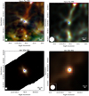 |
Fig. 10 As in Fig. 9, but for Haro 5a IRS (top) and HH 354 IRS (bottom). |
| In the text | |
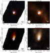 |
Fig. 11 As in Fig. 9, but for HH 381 IRS (top) and Parsamian 21 (bottom). |
| In the text | |
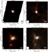 |
Fig. 12 As in Fig. 9, but for PP 13 S (top) and Re 50 N IRS 1 (bottom). |
| In the text | |
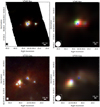 |
Fig. 13 As in Fig. 9, but for V346 Nor (top) and V733 Cep (bottom). |
| In the text | |
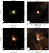 |
Fig. 14 As in Fig. 9, but for V883 Ori (top) and V1647 Ori (bottom). |
| In the text | |
|
Fig. 15 Continuum-subtracted spectra of PACS and SPIRE for Haro 5a IRS, HH 354 IRS, and HH 381 IRS. For the indicators of the lines, we use a 1.5−σ lower limit. |
| In the text | |
|
Fig. 16 Continuum-subtracted spectra of PACS and SPIRE for PP 13S, Re 50 N IRS/HBC 494, and V346 Nor. |
| In the text | |
|
Fig. 17 Continuum-subtracted Spectra of PACS and SPIRE for V883 Ori and V1647 Ori. |
| In the text | |
|
Fig. A.1 Line maps of PACS with visible lines for HH354 IRS. The maps show a specific bandwidth around emission lines of molecularor atomic transitions in the spectra coming from the integral field spectroscopy from PACS. The bandwidth is defined for each source by a fitting routine. A threshold cuts off noise below a specific value. For molecular lines, the species is mentioned in the upper left corner of the plot, together with the energy transition for CO and its isotopolog and the wavelength for other molecules. For the atomic lines, next to the isotope we give the frequency of the transition. The circle in each of the plots represents the coordinates of the optical FUor/EXor. |
| In the text | |
|
Fig. A.2 Line maps of PACS with visible lines for HH 381 IRS. |
| In the text | |
|
Fig. A.3 Line maps of PACS with visible lines for Parsamian 21. |
| In the text | |
|
Fig. A.4 Line maps of PACS with visible lines for PP 13 S. |
| In the text | |
|
Fig. A.5 Line maps of PACS with visible lines for Re 50 N IRS 1, part 1. |
| In the text | |
|
Fig. A.6 Line maps of PACS with visible lines for Re 50 N IRS 1, part 2. |
| In the text | |
|
Fig. A.7 Line maps of PACS with visible lines for V1647 Ori. |
| In the text | |
|
Fig. A.8 Line maps of PACS with visible lines for V346 Nor, part 1. |
| In the text | |
|
Fig. A.9 Line maps of PACS with visible lines for V346 Nor, part 2. |
| In the text | |
|
Fig. A.10 Line maps of PACS with visible lines for V733 Cep. |
| In the text | |
|
Fig. A.11 Line maps of PACS with visible lines for V883 Ori. |
| In the text | |
|
Fig. A.12 Line maps of SPIRE with visible lines for EX Lup. |
| In the text | |
|
Fig. A.13 Line maps of SPIRE with visible lines for Haro 5a IRS. |
| In the text | |
|
Fig. A.14 Line maps of SPIRE with visible lines for HH 354 IRS. |
| In the text | |
|
Fig. A.15 Line maps of SPIRE with visible lines for HH 381 IRS. |
| In the text | |
|
Fig. A.16 Line maps of SPIRE with visible lines for Parsamian 21. |
| In the text | |
|
Fig. A.17 Line maps of SPIRE with visible lines for PP 13 S. |
| In the text | |
|
Fig. A.18 Line maps of SPIRE with visible lines for Re 50 N IRS 1. |
| In the text | |
|
Fig. A.19 Line maps of SPIRE with visible lines for V1647 Ori. |
| In the text | |
|
Fig. A.20 Line maps of SPIRE with visible lines for V346 Nor, part 1. |
| In the text | |
|
Fig. A.21 Line maps of SPIRE with visible lines for V346 Nor, part 2. |
| In the text | |
|
Fig. A.22 Line maps of SPIRE with visible lines for V733 Cep. |
| In the text | |
|
Fig. A.23 Line maps of SPIRE with visible lines for V883 Ori. |
| In the text | |
Current usage metrics show cumulative count of Article Views (full-text article views including HTML views, PDF and ePub downloads, according to the available data) and Abstracts Views on Vision4Press platform.
Data correspond to usage on the plateform after 2015. The current usage metrics is available 48-96 hours after online publication and is updated daily on week days.
Initial download of the metrics may take a while.