| Issue |
A&A
Volume 631, November 2019
|
|
|---|---|---|
| Article Number | A163 | |
| Number of page(s) | 20 | |
| Section | The Sun | |
| DOI | https://doi.org/10.1051/0004-6361/201834625 | |
| Published online | 15 November 2019 | |
Hinode EIS line widths in the quiet corona up to 1.5 R⊙
1
DAMTP, Centre for Mathematical Sciences, University of Cambridge, Wilberforce Road, Cambridge CB3 0WA, UK
e-mail: This email address is being protected from spambots. You need JavaScript enabled to view it.
2
Udaipur Solar Observatory, Physical Research Laboratory, Badi Road, Udaipur 313 001, India
Received:
12
November
2018
Accepted:
29
September
2019
Abstract
We present an analysis of several Hinode Extreme-ultraviolet Imaging Spectrometer (EIS) observations of coronal line widths in the quiet Sun, up to 1.5 R⊙ radial distances. Significant variations are found, which indicates no damping of Alfvén waves in the quiescent corona. However, the uncertainties in estimating the instrumental width mean that a firm conclusion cannot be reached. We present a discussion of various EIS instrumental issues and suggest that the strongest lines, from Fe XII at 193.5 Å and 195.1 Å, have anomalous instrumental widths. We also show how line widths in EIS are uncertain when the signal is low, and that the instrumental variation along the slit is also uncertain. We also find an anomalous decrease (up to 40%) in the intensities of these lines in many off-limb and active region observations, and provide evidence that this is due to opacity effects. We find that the most reliable measurements are obtained from the weaker lines.
Key words: Sun: corona / techniques: spectroscopic
© ESO 2019
1. Introduction
It has long been known that coronal lines always exhibit non-thermal broadenings (see the recent review in Del Zanna & Mason 2018), that is, widths that are in excess of the expected thermal widths on the basis of the estimates of the ion temperatures. Earlier Skylab and Solar Maximum Mission (SMM) observations of coronal forbidden lines indicated excess widths of 15–20 km s−1 (see, e.g. Doschek & Feldman 1977; Mason 1990). This excess broadening is often interpreted as a signature of waves that propagate in the solar atmosphere and could contribute to the coronal heating (see, e.g. Hollweg 1978, 1984; Parker 1988; van Ballegooijen et al. 2011). Variations (both increases and decreases) in the excess broadening with height above the limb have been reported. The decreases in the excess broadening seen in coronal holes and quiet Sun areas have been interpreted to be caused by the damping of Alfvén waves in the corona.
We only consider here quiet Sun off-limb observations. There are surprisingly few observations with varying radial distance reported in the literature. The measurements are notoriously challenging as the signal rapidly decreases off-limb, and there is always a large uncertainty in measuring ion temperatures. Also, estimating instrumental broadenings is often a challenge in the extreme ultraviolet (EUV) and ultraviolet (UV). Doschek & Feldman (1977) measured the widths of several coronal iron UV forbidden lines above the limb and found excess widths of about 20 km s−1. Hassler et al. (1990) found increases in the excess widths of Mg X lines which were observed with a rocket spectrum. In contrast, off-limb observations with the Solar and Heliospheric Observatory (SoHO) Coronal Diagnostic Spectrometer (CDS) of the quiet corona showed a decrease in the line widths of Mg X (Harrison et al. 2002). However, an east-west variation of the CDS instrumental width was later found, thus removing evidence of variations (Wilhelm et al. 2005).
Most of the SoHO Solar Ultraviolet Measurement of Emitted Radiation (SUMER) off-limb observations of quiet regions have shown little variation in the excess line widths up to about 1.3 R⊙ (see Doyle et al. 1998; Doschek & Feldman 2000; Landi & Feldman 2003; Wilhelm et al. 2004). Seely et al. (1997) found a small decrease in the excess line widths from about 20 km s−1 near the limb to about 10 km s−1 up to about 1.2 R⊙, assuming uniform ion temperatures for all elements. Landi & Feldman (2003) performed a very detailed analysis, measured the ionisation temperatures, and found nearly constant excess line widths up to 1.3 R⊙. The values were higher than those found by Seely et al. (1997) though, being around 30 km s−1. Landi et al. (2006) instead found small increases, of up to 10 km s−1, in coronal lines observed by SUMER out to 1.6 R⊙.
In contrast, there are two reported Hinode Extreme-ultraviolet Imaging Spectrometer (EIS, see Culhane et al. 2007) off-limb observations of the quiet Sun where a decrease in the excess widths were found. Hahn & Savin (2014) measured widths along expected locations of magnetic field lines close to the solar limb, while Gupta (2017) analysed a “quiet” off-limb area close to an active region (which was the focus of an analysis by O’Dwyer et al. 2011).
As SUMER had a much better spectral resolution than CDS and EIS, we can summarise the previous observations by stating that there is no significant evidence for variations in the excess widths of coronal lines in the quiet Sun, out to about 1.3 R⊙. Our aim is to analyse further Hinode EIS observations and extend these results to greater heights.
Since pointing Hinode outside the solar limb is normally not allowed and the EIS slits are aligned in the N–S direction, most off-limb quiet Sun EIS observations have been restricted to about 1.2 R⊙. Here, we present results of a special EIS campaign where the EIS slit reached 1.5 R⊙, and with which we have used to assess line width variations up to such distances.
The paper is organised as follows: Sect. 2 presents a summary of the data analysis and a few instrumental issues relevant to this paper. Section 3 presents a sample of the results from this special EIS campaign. As we do not find strong evidence for a decrease in the line widths and find an anomalous behaviour in the strongest lines, in Sect. 4 we present the results of an additional analysis of the Gupta (2017) observations, in order to try and understand why different spectral lines provide different excess widths. We carry out an analysis of the possible reasons for this, which is summarised in Sect. 5 and detailed in an appendix. Section 6 presents our conclusions.
2. EIS data analysis and instrumental issues
The EIS data were processed with custom-written software (see, e.g. Del Zanna et al. 2011). The analysis closely follows the procedures developed within the EIS software. The hot, warm pixels, and those affected by cosmic rays or particle events, are flagged as “missing”. The missing pixels are then replaced with interpolated values with a series of interpolations along different directions. The exposures are then visually inspected. As the dark frames (bias) are extremely variable and unknown, a base minimum value is removed from each exposure (unlike the standard software where an average of the bottom pixels is removed – which causes negative data numbers (DN) in the spectra). A large quantity of dust on the EIS CCD affects the 193.5 Å line, so that area was excluded during the analysis. To obtain an uncertainty in each pixel, we converted the observed DN into detected photon events, assuming Poisson noise and adding the read-out noise.
In principle, saturation of an EIS pixel should occur at a value of 16 383 in data numbers (DN). Indeed the standard software assumes a saturation threshold of 16 000 DN. However, we have found some evidence for small non-linear behaviour in the line intensities when peak counts are above 8000–10 000 DN, as described in the Appendix.
The narrow 1″ and 2″ EIS slits are 1024 pixels (1 pixel is equal to about 1″) long, which are equivalent to about 1024″. However, when exposures are telemetred to the ground, only a portion of the slits (up to 512 pixels) is downloaded. Regular observations extract the central regions of the slits. A region of the Sun is scanned by “rastering”, obtained by moving the image of the slits onto the detectors in the E–W direction.
The images of the two narrow slits (1 and 2″) onto the detector present several instrumental issues which are different for the two slits. The main ones are a slant of the spectra compared to the detector pixels (Del Zanna & Ishikawa 2009), and a tilt and width of the spectral lines which vary with position along the slit. We have corrected the EIS full spectra for the slant and tilt by rotation, following the prescriptions in Del Zanna & Ishikawa (2009). We adopted the same procedure developed by W. Thompson for the SoHO CDS, which suffered similar instrumental issues as EIS. We first rotate the spectra. We note that once the spectra are rotated, a shift along the slit of about 18 EIS pixels has always been present. The spectra in the two EIS channels (short: SW and long: LW) are then corrected for the differences in the solar X and Y. In earlier observations, a shift of about 2″ in solar X was also present, meaning that the SW and LW spectra never observed simultaneously the same region on the Sun.
The cfit procedures (developed by S. V. Haugan for the SoHO CDS but modified by us) were used to fit Gaussian profiles and a linear background to the spectra in DN. As the EIS profiles are dominated by the instrumental width, they are always close to Gaussian, for the unblended strong lines which we consider here. We have also checked that the total signal obtained by summing the counts over the line profiles is close (within at most a few percent) to the value obtained from the Gaussian parameters (see the Appendix).
The radiometric calibration is only applied later to the integrated intensities. We used the Del Zanna (2013a) calibration, although some results obtained with the ground calibration (Lang et al. 2006) are also shown. We have also processed some of the observations presented here with the standard EIS software, and found very similar results.
Observed line widths are often expressed as full-width at half-maximum (FWHM) and typically contain an instrumental width, a thermal width which depends on the ion temperature, and an excess width ξ. Assuming thermal broadening:
 (1)
(1)
where wI is the instrumental FWHM, k is Boltzmann’s constant, M is the mass of the ion, and Ti the ion temperature.
As the widths of the EIS lines are dominated by the instrumental width, a careful assessment of instrumental issues should be carried out. A thorough discussion of the EIS instrumental width and its variation in time, along the two narrow slits and as a function of mirror position is beyond the scope of the present paper. However, here and in the Appendix we present some key examples which are relevant for this paper.
Hara et al. (2008) noted in their appendix that the instrumental widths of the EIS lines in the SW channel must be significantly larger than the values measured on the ground. In most literature, the instrumental widths as described in the EIS software note 4 (Young 2011) are used. They were obtained from observations in Nov.–Dec. 2009 and do not have a wavelength (or time) dependence. The main assumption was that the smallest observed widths would provide a measure of the instrumental width. The same observations were used to measure the tilt (Young 2010).
We have performed our own analyses and found some variations and differences with the values recommended in the EIS software notes. To illustrate the main effects relevant to this paper, we show in Fig. 1 the peak intensities, position and FWHM of the main SW lines from a 2″ slit observation on the quiet Sun obtained on 2006-10-28 at 11:17 UT (bottom 512 pixels of the 1024 pixel slit) and 11:23 UT (top 512 pixels of the slit) with 5 exposures. We selected the longest (160 s) exposures and rebinned the spectra by a factor of 3 along the slit to improve the signal. The dashed lines in the middle and bottom rows are the recommended values for the variation in the position and the instrumental FWHM estimated by P. R. Young from the Nov.–Dec. 2009 observations. It is clear that some departures from the recommended values are present. In particular, the slit width seems to be overestimated at places.
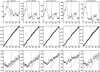 |
Fig. 1. Top row: peak DN in a selection of SW lines, as function of slit position, for 160 s exposure with 2″ slit on the quiet Sun, recorded on 2006-10-28. The dashed vertical line indicates the mid position of the 1024 slit. Middle row: line centroid positions (Å); the dashed line indicates the estimated variation as available in the EIS software notes. Bottom row: FWHM (Å) in the lines, while the dashed line indicates the estimated variation as available in the EIS software notes. The bottom axis is the position along the slit, from bottom (pixel 0) to the top (pixel 1023). |
The first main point of Fig. 1 is to show that the bottom of the 1024″ slit has a much lower width than the central and top regions where the width increases. The initial decrease and then increase in the bottom of the slit is not obvious in other datasets (cf. the Appendix) and is within the scatter of the measurements, which is typically around 3 mÅ. The fact that the bottom is the best part of the slit is the main reason why the special off-limb sequence discussed below was designed to obtain data from this region of the CCD.
The second main point of the figure is to show that the widths of the three Fe XII 192.4, 193.5, and 195.1 Å lines are consistently different at all locations along the slit. The widths of the 193.5 and 195.1 Å lines are similar, while the width of the 192.4 Å line is smaller by about 4–5 mÅ, as shown in Fig. 2. We have seen similar differences in the observations we have analysed, as shown in the Appendix. Lines at shorter and longer wavelengths show widths similar to the weaker Fe XII 192.4 Å line, as for the Fe X and Fe XIII lines shown in Fig. 1.
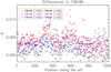 |
Fig. 2. Differences in the FWHM of the three main Fe XII lines, as a function of the position along the slit, for the same observation in Fig. 1. |
We cannot think of any physical reason that can explain the differences in the widths of the Fe XII lines. The EIS wavelength range is rich in unidentified coronal lines, as discussed in Del Zanna (2012). However, these are typically much weaker (a few percent) than the strong Fe XII lines. Also, recent laboratory measurements with an Electron Beam Ion Trap (EBIT) do not suggest that lines from other ions or elements are blending the Fe XII lines, see Träbert et al. (2014). We would therefore expect the widths of these three Fe XII lines to be the same.
Indeed there is an independent evidence for this. To our knowledge, the best measurements of the widths of these lines were obtained in second order with the SERTS-95 sounding rocket (Brosius et al. 1998). The spectrometer had an instrumental FWHM resolution of about 30 mÅ in second order. In their quiet Sun averaged spectra the 193.5 and 195.1 Å lines actually had lower observed widths than the 192.4 Å line, however the signal was low, and measurements had a large uncertainty. In the active region spectra, the observed FWHM for the 192.4, 193.5 and 195.1 Å lines were 51.2 ± 3, 49.2 ± 3, and 49.3 ± 3 mÅ respectively, so in fact were the same within uncertainties. We conclude that the larger widths in the two EIS Fe XII lines (193.5, and 195.1 Å) are instrumental.
Finally, on the basis of the east-west variation in the instrumental line widths found in SoHO CDS, we have carried out several tests on observations of the quiet Sun with the 2″ slit to see if any east-west instrumental variation is also present for Hinode EIS. We analysed both the central part of the slit, and in particular the bottom of the 2″ slit, as the main scientific results presented here were obtained with that part of the slit. We did not find any obvious variations, as shown in the Appendix.
3. The off-limb QS observations out to 1.5 R⊙
One of us (GDZ) designed an engineering EIS “study” (gdz_off_limb1_60) to use the bottom half of the long (1024″) EIS slit, so the lower part of the EIS field of view could reach 1.5 R⊙. A week-long campaign (Hinode HOP 7) was coordinated to obtain simultaneous SOHO/Hinode/TRACE/STEREO observations during the SOHO-Ulysses quadrature in May 2007. EIS observations were obtained during May 7–10, as outlined in Del Zanna et al. (2009). The EIS 2″ slit was moved with 8″ jumps, to cover about 500″ in the E-W direction with 60 s exposures. As far as we are aware, these are the only EIS observations of the quiet Sun up to such large distances above the limb.
The Sun was very quiet during the campaign, with the exception of an active region (AR), which was at the west limb on May 7. The AR produced a filament eruption, where large non-thermal widths of more than 100 km s−1 were observed (Del Zanna et al. 2009). On May 10, the main part of the active region was behind the limb, as shown in Fig. 3. Some emission associated with the active region is still visible in the north portion of the EIS field of view, but the lower part was quiet. An off-limb region about 5° wide, along the radial sector indicated in Fig. 3 was chosen to obtain averaged spectra, to improve the signal in the far off-limb region.
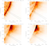 |
Fig. 3. Monochromatic images (negative) in a few spectral lines, obtained on 2007-05-10 with Hinode EIS. The radial sector used to obtain averaged spectra in the quiet corona as a function of radial distance is indicated. |
A detailed analysis of temperatures and densities obtained from this region has been presented in Del Zanna et al. (2018). A remarkable feature was the nearly constant ionisation temperature (around 1.4 MK) obtained from ratios of Fe X, Fe XI, Fe XII lines, extending to greater heights the SUMER results of Landi & Feldman (2003). The densities were close to typical quiet Sun values, and scattered light in the coronal lines was found to be negligible.
The signal in the Fe XII 195.1 Å was sufficient to measure its width for each pixel, at least out to about 1.2 R⊙, as shown in Fig. 4. There is an indication of a variation in the width, but with a large scatter, largest at greater distances, where the signal is low, below about 200 DN in the peak of the line (cf. bottom plot in Fig. 4). This is expected, as the width of weak line profiles tends to increase. In the Appendix, we show several examples of near-simultaneous observations with different exposure times, where it is clear that a large uncertainty (5 mÅ or more) is associated with the widths of lines with peak counts below 200 DN, as seen here. We note that we have not constrained the upper limit of the width of the line during the fitting process.
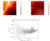 |
Fig. 4. Selected results from the Hinode EIS off-limb observation on 2007-05-10 at 10:21 UT. Top: images of the peak intensity (DN) and FWHM (mÅ) in the Fe XII 195.1 Å line. Bottom: scatter plot of the FWHM (Å) as a function of peak intensity. |
Figure 5 shows the variation in the widths of the Fe XII 195.1, 193.5 Å, and Fe XIII 202 Å lines as a function of radial distance, obtained from the radial QS sector shown in Fig. 3. The Fe XII 193.5 Å and Fe XIII 202 Å lines do not show any significant variations in their widths. We note the instrumental effect: the widths of the two strong Fe XII lines are larger than that of the Fe XIII line. The weaker Fe XII 192.4 Å line is not shown in the plot as this line was not included in the EIS study. Another feature is the increased width of the Fe XII 195.1 Å line near the limb. Below we present similar results, which we suggest are related to opacity effects.
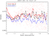 |
Fig. 5. FWHM of the Fe XII 195.1, 193.5 Å and Fe XIII 202 Å lines, obtained from averaged spectra along the radial QS sector shown in Fig. 3. The points are the pixel-by-pixel FWHM of the 195.1 Å line. |
The points in Fig. 5 are the single values obtained for the Fe XII 195.1 Å line from each EIS pixel used to obtain the averaged spectra, and give an indication of the large uncertainty associated with such measurements (5 mÅ or more in the weaker off-limb areas). The variations in the widths obtained from the averaged spectra are within 3 mÅ, that is well within the large scatter in each pixel values and also within the uncertainties in the small variation of the instrumental width in the bottom of the CCD, shown above and further discussed in the Appendix.
To illustrate the challenge in obtaining the excess widths, we plot in Fig. 6 the values obtained from the Fe XIII 202 Å line, subtracting a thermal width (assuming T = 1.4 MK as measured from line ratios) and two different instrumental widths. A constant value of 0.064 Å (triangles) provides excess widths around 15–20 km s−1, close to some of the Skylab and SUMER results (see, e.g. Seely et al. 1997). The error bars on the points are obtained by varying the instrumental width by only ±2 mÅ, which is well within the scatter of values we have seen in several observations, and adding a ±2 mÅ uncertainty in the observed widths. The boxes are the values obtained with the instrumental width variation as obtained by P. R. Young (discussed previously) and available within the EIS software. The latter instrumental widths suggest a small decrease at heights greater than 1.3 R⊙, although in several places they produce negative excess widths (whenever the observed width was smaller than the sum of the thermal and instrumental widths, we have set the values of the excess width to zeros in the plot).
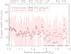 |
Fig. 6. Excess widths from the Fe XIII 202 Å line as a function of radial distance, obtained from the radial QS sector shown in Fig. 3, assuming two different instrumental widths. |
We have analysed the observations of the week-long campaign, and found similar results, as shown in the Appendix for May 8 (see Figs. G.1 and G.2). In this case, a marginal increase in the excess widths above 1.3 R⊙ is present.
As most of the 2007 observations were affected somewhat by the presence of the active region, we have recently obtained new observations, in July 2018, when the Sun was very quiet. The pointing was similar to the 2007 observations, in the south-west. As the EIS instrument has degraded and the solar signal is lower, these observations have lower quality than the earlier ones. In this case we also found line widths to be nearly constant, as shown in the Appendix.
Therefore, we conclude that, in agreement with the SUMER results, there is no significant evidence for a variation of the excess widths by more than 10 km s−1 out to 1.3 R⊙. The uncertainties in the observed and instrumental widths preclude firm conclusions in the 1.3–1.5 R⊙ region.
4. A case study: the 2007-12-17 off-limb observation
We have further analysed the same “quiet Sun” off-limb region considered by Gupta (2017), consisting of an E–W region out to 1.25 R⊙ and 30″ wide in the N–S direction. The excess widths measured by Gupta (2017) showed several inconsistencies. The widths of the strongest Fe XII lines were known to be different, although this was not illustrated in the paper. As this was an excellent observation with many spectral lines and good signal, we have considered it as a case study, to explore the instrumental and anomalous effects in the Fe XII lines.
The FWHM of the three strongest Fe XII lines are shown in Fig. 7. Both the single pixel values and the values obtained from the averaged spectra are shown. The FWHM of the weaker 192 Å line has a small decrease (2 mÅ) with radial distance. The nearly constant line widths in the weaker Fe XII line are in agreement with the widths of other lines: the strongest Fe XIII line, at 202 Å also shows a nearly constant FWHM with radial distance, see Fig. 8 (top). In the LW channel, the Fe XV line at 284 Å also indicates a nearly constant line width, although with a larger scatter. The increase in the width of the Fe XV line near the limb could be due to blending with an Al line nearby affecting the measurements, or more probably with opacity effects.
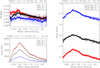 |
Fig. 7. Left: off-limb variations of the FWHM in the three Fe XII lines, obtained from a “quiet” region 30″ wide observed on 2007-12-17 (see Gupta 2017); variations of the peak line intensities (DN). Right: variations of the calibrated intensity line ratios, with the expected values shown as dashed lines. |
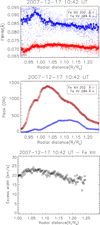 |
Fig. 8. Off-limb variations of the FWHM and peak line intensities for the strongest Fe XIII and Fe XV lines along the same “quiet” region 30″ wide as observed on 2007-12-17 and as on Fig. 7 (top and middle plot). Bottom plot: excess width in the Fe XIII line. |
Figure 8 (bottom) shows the excess width in the Fe XIII 202 Å line. As we have no indications (see also the Appendix) that the instrumental width varies along the E–W direction, its estimated value was subtracted (assuming the standard value in the EIS software, along with its thermal width, assuming an ion temperature of 1.8 MK. During this further analysis we found a software bug in the calculation by Gupta (2017), with the result that all the excess widths were overestimated by about 50%.
Returning to Fig. 7, we can clearly see two problems. One is that the instrumental widths of the stronger Fe XII lines are larger, as we have seen. The second is that the widths of 193 and 195 Å lines increase where the peak intensities are large, near the solar limb. The width of the stronger 195 Å line increases even more than the 193 Å line.
As already mentioned, we would expect the widths of these three lines to be the same. Furthermore, the intensity ratios of these lines, also shown in Fig. 7, vary with radial distance, contrary to their expected values, indicated with dashed lines. After an analysis of several observations, discussed below and in the Appendix, we found this anomalous behaviour to be typical and suggest that these variations are related to opacity effects in the stronger lines, as discussed below.
5. The anomalous Fe XII intensity ratios
We have seen that in certain places there appears to be some correlation between anomalous widths of the strongest Fe XII 193.5 and 195.1 Å lines, and anomalous intensities, when compared to the weaker 192.4 Å line. As these lines are the strongest features in the EIS spectra, being close to the peak of the EIS effective area, they are commonly used in the literature for a wide range of measurements, including line widths, electron densities and temperatures. We therefore explored these anomalies by analysing several datasets.
The ratios of the Fe XII 192.4, 193.5, and 195.1 Å lines are not sensitive to density or temperature. Del Zanna & Mason (2005) identified in laboratory plates obtained by B. C. Fawcett a weak density-sensitive line blending the 195.1 Å line. This transition is less than 1% the intensity of the strong line at typical quiet Sun densities, so can be ignored. At active region densities, this line can reach a 10% level, and the line profile becomes asymmetric.
Comparison with the well-calibrated Malinovsky & Heroux (1973) intensities shows exact agreement (within less than 1%) in the ratios of these Fe XII lines with theory (Del Zanna et al. 2012), as discussed in Del Zanna (2013a). One would therefore expect that these three lines should have a constant intensity ratio, with the exception of active region observations where the intensity of the 195.1 Å line should increase.
The 192/195 Å and 192/193 Å intensity ratios are in excellent agreement with the expected values in the dimmest regions for the earlier EIS observations. This is because the Del Zanna (2013a) calibration was based on earlier quiet Sun observations. With the ground calibration, the ratios are consistently lower by up to 15%. On a side note, in later observations the ratios have often shown decreases (by up to 30%), which would indicate a wavelength-dependent change in the sensitivity over time.
The anomalous behaviour in the intensity ratios is often associated with a broadening of the strongest lines, which in principle could be indicative either of an instrumental non-linear effect in the line cores or opacity. However, this anomalous behaviour does not seem to be related to a possible non-linearity in the EIS detector. We analysed several SYNOP1 studies, where two consecutive exposures, of 30 s and 90 s, are taken with the 1″ slit. In most cases we found that the anomalous ratios were the same in both exposures. If the reason for the variation in the ratio were due mainly to a non-linearity in the detector, the ratios should be different.
We can also rule out any blending in the strongest lines as it would increase their signal, and not decrease it. One effect which would naturally cause these anomalous ratios is opacity. Optical depth effects in coronal lines have rarely been reported, although they are known to be present in low-temperature lines formed in high-density regions or close to the solar limb.
The departures of the line ratios show a clear correlation with the intensities of the lines. As shown with some examples below and in the Appendix, we have found such departures in both 1 and 2″ slit spectra, in on-disk and off-limb spectra. These departures are normally larger (of the order of 30–40%) in observations where the peak intensities are above 2000 DN, and are more prominent in off-limb and active region observations.
These anomalous ratios have gone un-noticed in the literature, but we have found them in earlier (from 2006) and recent observations. The strongest departures occur where the lines are bright, independent of the slit used, the pointing (e.g. on-disk, at the limb or off-limb), and the source region (e.g. quiet Sun or active region).
We present here two examples, one on a quiet Sun off-limb observation, and one on an active region. More examples are presented in the Appendix.
5.1. Off-limb quiet Sun
Figure 9 summarises the main results obtained from a quiet Sun east limb observation with an ATLAS_60 study, recorded on 2013-02-14 at 09:49 UT with 60 s exposures. There were no active regions nearby, but the Sun was relatively active during this period, so the strongest 195 Å line was almost saturated near the limb, reaching a peak of 10 000 DN, as shown in Fig. 9, top plot. The 192/195 Å intensity ratio is close to the expected value in the dimmest regions (on-disk and far off-limb), but shows an anomalous behaviour in the brightest regions close to the limb. The 192/195 Å intensity ratio varies by as much as 35%. We note that the intensity variations are also related to an increase in the width of the 195 Å line. Similar behaviour is seen in the 192/193 Å ratio (not shown).
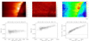 |
Fig. 9. Quiet Sun east limb observation on 2013-02-14 at 09:49 UT. Top images: peak intensity of the 195 Å line (DN), the observed FWHM (Å) of the 192 Å line, and the intensity ratio of the 192 and 195 Å lines. The coordinates are the pixel positions. The arrows indicate two regions, off-limb (OL) and on-disk (OD) chosen for further studies. Lower plots: scatter plots of the FWHM in the 192 and 195 Å lines, as a function of their peak intensity, and the intensity ratio of the 192/195 Å lines. The dashed line indicate the expected value. |
We have selected two regions in the EIS spectra, indicated with “OL” (off-limb, 5 × 7 pixels) and “OD” (on-disk, 3 × 4 pixels) and shown in Fig. 9. We averaged spectra in these two regions, and measured the line intensities. Using the Del Zanna (2013a) calibration, we find excellent agreement (within a few percent) among the intensities of the Fe XII lines in the on-disk case, as shown in Fig. 10 (top). The figure shows the emissivity ratio plots (cf. Del Zanna & Mason 2018), whereby the intensities of the lines are divided by their emissivities. If the plasma along the line of sight is iso-density, the curves should provide a crossing. The crossing indicated for the on-disk quiet Sun an electron density of 108.5 cm−3. For the off-limb case, the weaker lines indicate a far higher density of 108.8 cm−3, as one would expect as this is a much brighter region. The anomaly in the 193.5 and 195.1 Å lines is obvious.
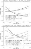 |
Fig. 10. Emissivity ratio plots for the main Fe XII lines in the on-disk (top) and off-limb (bottom) regions indicated in Fig. 9. The calibrated intensities (in photons cm−2 s−1 arcsec−2) are shown in the plots (Iob). |
We then performed a DEM analysis of the off-limb region using CHIANTI v.8 (Dere et al. 1997; Del Zanna et al. 2015) and a selection of lines, see Fig. 11. The peak emission is close to the temperature of formation of Fe XII in ionisation equilibrium, and there is very little emission at higher temperatures. The Sulphur and Iron lines indicate photospheric abundances (Asplund et al. 2009).
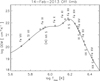 |
Fig. 11. DEM distribution for the off-limb region indicated in Fig. 9. The points indicate the ratio of the predicted versus observed radiance, multiplied by the DEM value at the temperature of maximum emissivity in each line. |
The contribution function of the Fe XII lines indicates that they are sensitive to temperatures in the 1–2.2 MK range. Integrating the DEM distribution over this temperature range, we obtain a column emission measure EM of 8.8 × 1027. Assuming a uniform distribution of the densities along the line of sight (filling factor unity), and the measured density (108.8 cm−3), we obtain a path length of 1.8 × 1010 cm. As the absolute calibration of the EIS instrument appears correct within 20% (Del Zanna 2013a), the main uncertainty in this estimate is the absolute value of the Iron abundance. If its value was for example higher by a factor of two, the EM would be a factor of two lower, and the path length would be 1010 cm.
The optical thickness at line centre for a spectral line is (cf. Del Zanna & Mason 2018):
 (2)
(2)
where kν0 is the absorption coefficient at line centre (at frequency ν0), Nl is the number density of the lower level, and ΔS the path length. If photons are scattered within a Doppler profile, that is, with a Gaussian function in frequency with a half-width ΔνD, the optical thickness at line centre is
 (3)
(3)
where flu is the absorption oscillator strength, c is the speed of light, me the electron mass. In terms of wavelengths, the Doppler width of a line, equivalent to the half-width ΔνD, is  , where ΔλFWHM is the measured FWHM of the line profile in wavelength. So the optical thickness at line centre can be written as
 (4)
(4)
with λ and ΔλFWHM expressed in Å. For the 195 Å line, flu = 2.97/4, neglecting the weaker line blending the main line.
The population of the lower level can be written as
 (5)
(5)
where Nl/N(Fe XII) = 0.9 is the relative population of the ground state at quiet Sun densities, N(Fe XII)/N(Fe) = 0.25 is the peak relative population of the ion, Ab(Fe) = 3.16 × 10⁻⁵ is the Fe photospheric abundance, NH/Ne = 0.83, and Ne is the averaged electron number density. We therefore have τ0 = 6.9 × 10⁻²⁰ Ne ΔS [cm−2] assuming ΔλFWHM = 0.02 Å.
With the measured averaged density of 7 × 108 cm−3, and assuming the path length obtained from the emission measure (1.8 × 1010 cm), we obtain τ0 = 0.87, which is a significant optical thickness at line centre for the 195 Å line. We note that the 192.4 Å line has an oscillator strength a third of the 195.1 Å line (flu = 0.98/4), so has a smaller opacity at line centre, 0.29.
To estimate how an opacity at line centre of 1 for the 195.1 Å line could affect the 195/192 Å intensity ratio, we assume that the source function Sν(τν) does not vary along the line of sight, and take averaged values of all the quantities. Of course Sν(τν) would depend at each location on the local angle-averaged intensity Jν, even if the plasma is uniformly distributed in density. We note that this simple approach is essentially the same as the widely-used one involving averaged escape factors. Obviously, a proper analysis would require a model of the spatial distribution of the density.
With this assumption, the peak intensity of each line is
 (6)
(6)
while the line source function Sν is:
 (7)
(7)
with standard notation. If we calculate, assuming optically thin conditions, the relative populations of the two upper levels producing the 195, 192 Å lines, we find that S195/S192 = 1.04. The I195/I192 ratio of the peak intensities of the two lines for negligible opacity is 3.2. For τ0(195) = 1 we have I195/I192 = 2.2, so we obtain a 0.7 reduction in the intensity ratio, which is similar to the observed value, 0.74 (using the Del Zanna 2013a calibration, the I192/I195 ratio in OL is 0.42).
5.2. Active region on-disk
Young et al. (2009) reported an analysis of EIS Fe XII line ratios to measure electron densities, but also showed in an Appendix the same Fe XII intensity ratios discussed here. They noted a variation of the ratios along the slit and suggested that perhaps this was due to a change in the instrument sensitivity along the slit. We re-analysed their 2007 May 6 observation and found that also in this case the 192/195 Å intensity ratio varies with the intensity of the lines by about 30%.
This was an early observation of an active region on 2007 May 6, with the 1″ slit and 40 s exposures. Young et al. (2009) reported line ratios along the slit for a single exposure. The chosen exposure is probably the No. 204 (counted from the east, over 330 exposures). Figure 12 (top) shows the logarithmically-scaled intensity of the strongest lines, as in Fig. 12 of Young et al. (2009), showing reasonable agreement (changing the exposure within a few pixels provides similar results). Figure 12 (middle) shows the 192/195 Å and 193/195 Å intensity ratios, using the EIS ground calibration. These ratios are virtually the same as those shown in Fig. B.1 in Young et al. (2009). The drop around pixel 220 in the 193/195 Å ratio is caused by a large piece of dust present on the EIS CCD at that location where the 193 Å line is.
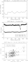 |
Fig. 12. Top: logarithmically-scaled intensity of the Fe XII 195 Å line along 304″ of the 1″ slit, across AR loops observed on 2007 May 6, as in Fig. 12 of Young et al. (2009). Middle: intensity ratios of the Fe XII lines, using the ground calibration. Bottom: intensity ratio of the Fe XII 192 versus 195 Å lines as a function of the peak intensity in the stronger line, and for two different radiometric calibrations. |
It turns out that the increased ratio noted by Young et al. (2009) was in a bright region in the top region. Figure 12 (bottom) shows the Fe XII 192/195 Å intensity ratio this time plotted as a function of the peak intensity of the 195 Å line, showing the clear trend which we have seen in most active region observations. The variation is significant, about 30%. The pluses in Fig. 12 are obtained with the EIS ground calibration, while the boxes are with the Del Zanna (2013a) calibration. As we have already mentioned, the Del Zanna (2013a) calibration was obtained assessing line ratios in quiet Sun areas in 2006−2007 in this wavelength region, hence provides a very good agreement with the expected values in the low-intensity areas in active regions.
The ratios have the same behaviour across the whole active region. Figure 13 shows the central part of the EIS raster, in the core of an active region. The brightest region is moss. The 192/195 Å intensity ratio increases in the moss areas. The width of the 195 Å line is also increased in the same areas. We have selected a moss area well away from saturation, at raster position 141, 142 and position along the slit between 159 and 162 pixels. Here, the 192/195 Å intensity ratio is 0.37 instead of the optically-thin value of 0.31, so the 195 Å intensity is reduced by a factor of 0.84.
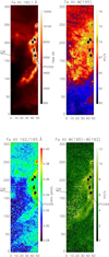 |
Fig. 13. Top: peak intensity (DN) and FWHM (km s−1) of the 195 Å line, with pixels above 12 000 blanked. Bottom: 192/195 Å intensity ratio (phot), and difference between the FWHM of the 195 and 192 Å lines (km s−1). Two regions selected for further analysis, on a moss and a quiet region (QR) within the active region are shown. |
The emissivity ratio plot shown in Fig. 14 (top) indicates, assuming that the 192 Å line is not affected by opacity, a density of 8 × 109 cm−3. The densities obtained from other ions such as Fe XIII, Fe XI, and Si X are slightly lower, around log Ne = 9.4−9.6. We have performed a DEM analysis on this moss region, adopting the coronal abundances obtained by Del Zanna (2013b), as they best reproduce the low-FIP versus high-FIP ions (the Fe abundance is 10−4 the H abundance). The total column EM = 2.3 × 1028 cm−5 within 1–3 MK. Assuming the Fe XII density, a path length of 3.6 × 108 cm is obtained. With a ground state population of 0.55, the ion abundance of 0.25 and ΔλFWHM = 0.02, we obtain that the optical thickness at the 195 Å line centre is 0.39. With the above assumption of constant line sources, and considering that the optical thickness of the 192 Å line is a third, we obtain that the 195/192 Å intensity ratio would be 2.75 instead of the optically-thin value of 3.2, corresponding to a 0.86 reduction, very close to the observed ratio of 0.84. If instead we adopted a lower density of 3 × 109 cm−3, we obtain an optical thickness at the 195 Å line centre of 1.2, with a corresponding estimated decrease in the 195/192 Å intensity ratio of 0.7.
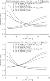 |
Fig. 14. Emissivity ratio plots for the main Fe XII lines in the moss and quiet regions indicated in Fig. 13. The calibrated intensities (in photons cm−2 s−1 arcsec−2) are shown in the plots (Iob). |
The active region area outside the moss region has a much lower electron density, around 1.6 × 109 cm−3 as shown in Fig. 14 (bottom). In this case, the diagnostics from other ions such as Fe XIII, Fe XI, and Si X are similar. Integrating the DEM over the 1–3 MK range, we obtain EM = 1.95 × 1027 cm−5 and a path length of 7.6 × 108 cm. The optical thickness at the 195 Å line centre is then 0.19, corresponding to an estimated decrease in the 195/192 Å intensity ratio by only 8%, relative to the optically-thin value.
6. Conclusions
The quiet Sun off-limb observations we have analysed do not indicate any significant variation in the widths of the coronal lines, up to 1.5 R⊙. Some variations are present, but they are within the uncertainties of these very difficult measurements, so we cannot confirm that there is any damping of Alfvén waves in the lower quiescent corona.
Our results, which extend out to 1.5 R⊙, indicate excess widths around 15–20 km s−1, and confirm those obtained from Skylab and SUMER in quiet Sun areas where no significant changes in excess line widths were found. A further analysis of the quiet Sun observations out to 1.2 R⊙ described in Gupta (2017) also indicates very small variations in the excess widths, with values also around 15–20 km s−1 (the previously published results were overestimated).
We look forward to the future measurements in the forbidden lines which will be obtained by DKIST. They will have a much greater accuracy in line width measurements, and will provide a range of diagnostics (see e.g. Del Zanna & DeLuca 2018).
We have carried out an analysis of several EIS datasets and found that the widths of the two strongest Fe XII lines are consistently larger than expected, and we suggest that this is an instrumental issue. We point out that these lines have been widely used in the literature to measure excess widths.
We found a wide-spread anomalous behaviour of the intensity ratios of the Fe XII lines in most off-limb and active region observations, and have provided evidence that the two strongest lines are affected by opacity. Opacity effects are very common in transition region lines, but have rarely been reported in coronal lines. There were several papers discussing the possibility of scattering of the strongest Fe XVII line at 15 Å in X-ray observations of active regions (see, e.g. Schmelz et al. 1997). However, most of the discrepancies were due to atomic data and/or blending (see Del Zanna 2011). Kastner & Bhatia (2001) report an analysis of opacity in the resonance Fe XV line at 284.16 Å, and suggested that the line intensity was increased due to opacity in some active region observations.
The fact that Fe XII lines are often affected by opacity has several implications. On a positive note, the ability to measure the optical thickness, in conjunction with an independent measurement of the electron density via line ratios (using weaker lines or other ions), gives us the possibility to estimate the path lengths of the sources.
On a negative note, these opacity effects and anomalous behaviour of the two strongest Fe XII lines most likely affect several published results. We have also found evidence that strong lines from other ions are also affected by opacity, so previous results based on widths and intensities (e.g. densities, emission measures) of the strongest lines, especially in off-limb observations, active regions and flares should be revisited.
Acknowledgments
GDZ and HEM acknowledge support by STFC (UK) via a consolidated grant to the solar/atomic physics group at DAMTP, University of Cambridge. GRG acknowledges support from the UK Commonwealth Scholarship Commission via a Rutherford Fellowship. We warmly thank the effort of all the EIS team members involved in the planning of EIS observations with the engineering study. We thank the anonymous referee for several useful suggestions which helped to improve the paper. Hinode is a Japanese mission developed and launched by ISAS/JAXA, with NAOJ as domestic partner and NASA and STFC (UK) as international partners. It is operated by these agencies in co-operation with ESA and NSC (Norway). CHIANTI is a collaborative project involving the University of Cambridge (UK), George Mason University, and the University of Michigan (USA).
References
- Asplund, M., Grevesse, N., Sauval, A. J., & Scott, P. 2009, ARA&A, 47, 481 [NASA ADS] [CrossRef] [Google Scholar]
- Brosius, J. W., Davila, J. M., & Thomas, R. J. 1998, ApJS, 119, 255 [NASA ADS] [CrossRef] [Google Scholar]
- Culhane, J. L., Harra, L. K., James, A. M., et al. 2007, Sol. Phys., 243, 19 [Google Scholar]
- Del Zanna, G. 2011, A&A, 536, A59 [NASA ADS] [CrossRef] [EDP Sciences] [Google Scholar]
- Del Zanna, G. 2012, A&A, 537, A38 [NASA ADS] [CrossRef] [EDP Sciences] [Google Scholar]
- Del Zanna, G. 2013a, A&A, 555, A47 [NASA ADS] [CrossRef] [EDP Sciences] [Google Scholar]
- Del Zanna, G. 2013b, A&A, 558, A73 [NASA ADS] [CrossRef] [EDP Sciences] [Google Scholar]
- Del Zanna, G., & DeLuca, E. E. 2018, ApJ, 852, 52 [NASA ADS] [CrossRef] [Google Scholar]
- Del Zanna, G., & Ishikawa, Y. 2009, A&A, 508, 1517 [NASA ADS] [CrossRef] [EDP Sciences] [Google Scholar]
- Del Zanna, G., & Mason, H. E. 2005, A&A, 433, 731 [NASA ADS] [CrossRef] [EDP Sciences] [Google Scholar]
- Del Zanna, G., & Mason, H. E. 2018, Liv. Rev. Sol. Phys., 15, 5 [CrossRef] [Google Scholar]
- Del Zanna, G., Andretta, V., Poletto, G., et al. 2009, in The Second Hinode Science Meeting: Beyond Discovery-Toward Understanding, eds. B. Lites, M. Cheung, T. Magara, J. Mariska, & K. Reeves, ASP Conf. Ser., 415, 315 [NASA ADS] [Google Scholar]
- Del Zanna, G., O’Dwyer, B., & Mason, H. E. 2011, A&A, 535, A46 [NASA ADS] [CrossRef] [EDP Sciences] [Google Scholar]
- Del Zanna, G., Storey, P. J., Badnell, N. R., & Mason, H. E. 2012, A&A, 543, A139 [NASA ADS] [CrossRef] [EDP Sciences] [Google Scholar]
- Del Zanna, G., Dere, K. P., Young, P. R., Landi, E., & Mason, H. E. 2015, A&A, 582, A56 [NASA ADS] [CrossRef] [EDP Sciences] [Google Scholar]
- Del Zanna, G., Raymond, J., Andretta, V., Telloni, D., & Golub, L. 2018, ApJ, 865, 132 [Google Scholar]
- Dere, K. P., Landi, E., Mason, H. E., Monsignori Fossi, B. C., & Young, P. R. 1997, A&AS, 125, 149 [NASA ADS] [CrossRef] [EDP Sciences] [Google Scholar]
- Doschek, G. A., & Feldman, U. 1977, ApJ, 212, L143 [CrossRef] [Google Scholar]
- Doschek, G. A., & Feldman, U. 2000, ApJ, 529, 599 [NASA ADS] [CrossRef] [Google Scholar]
- Doyle, J. G., Banerjee, D., & Perez, M. E. 1998, Sol. Phys., 181, 91 [NASA ADS] [CrossRef] [Google Scholar]
- Gupta, G. R. 2017, ApJ, 836, 4 [NASA ADS] [CrossRef] [Google Scholar]
- Hahn, M., & Savin, D. W. 2014, ApJ, 795, 111 [NASA ADS] [CrossRef] [Google Scholar]
- Hara, H., Watanabe, T., Matsuzaki, K., et al. 2008, PASJ, 60, 275 [NASA ADS] [Google Scholar]
- Harrison, R. A., Hood, A. W., & Pike, C. D. 2002, A&A, 392, 319 [NASA ADS] [CrossRef] [EDP Sciences] [Google Scholar]
- Hassler, D. M., Rottman, G. J., Shoub, E. C., & Holzer, T. E. 1990, ApJ, 348, L77 [NASA ADS] [CrossRef] [Google Scholar]
- Hollweg, J. V. 1978, Rev. Geophys. Space Phys., 16, 689 [NASA ADS] [CrossRef] [Google Scholar]
- Hollweg, J. V. 1984, ApJ, 277, 392 [NASA ADS] [CrossRef] [Google Scholar]
- Kastner, S. O., & Bhatia, A. K. 2001, ApJ, 553, 421 [NASA ADS] [CrossRef] [Google Scholar]
- Landi, E., & Feldman, U. 2003, ApJ, 592, 607 [NASA ADS] [CrossRef] [Google Scholar]
- Landi, E., Feldman, U., & Doschek, G. A. 2006, ApJ, 643, 1258 [NASA ADS] [CrossRef] [Google Scholar]
- Lang, J., Kent, B. J., Paustian, W., et al. 2006, Appl. Opt., 45, 8689 [NASA ADS] [CrossRef] [PubMed] [Google Scholar]
- Malinovsky, L., & Heroux, M. 1973, ApJ, 181, 1009 [NASA ADS] [CrossRef] [Google Scholar]
- Mason, H. E. 1990, in IAU Colloq. 115: High Resolution X-ray Spectroscopy of Cosmic Plasmas, eds. P. Gorenstein, & M. Zombeck, 11 [Google Scholar]
- O’Dwyer, B., Del Zanna, G., Mason, H. E., et al. 2011, A&A, 525, A137 [NASA ADS] [CrossRef] [EDP Sciences] [Google Scholar]
- Parker, E. N. 1988, ApJ, 330, 474 [Google Scholar]
- Schmelz, J. T., Saba, J. L. R., Chauvin, J. C., & Strong, K. T. 1997, ApJ, 477, 509 [NASA ADS] [CrossRef] [Google Scholar]
- Seely, J. F., Feldman, U., Schühle, U., et al. 1997, ApJ, 484, L87 [NASA ADS] [CrossRef] [Google Scholar]
- Träbert, E., Beiersdorfer, P., Brickhouse, N. S., & Golub, L. 2014, ApJS, 215, 6 [NASA ADS] [CrossRef] [Google Scholar]
- van Ballegooijen, A. A., Asgari-Targhi, M., Cranmer, S. R., & DeLuca, E. E. 2011, ApJ, 736, 3 [NASA ADS] [CrossRef] [Google Scholar]
- Wilhelm, K., Dwivedi, B. N., & Teriaca, L. 2004, A&A, 415, 1133 [NASA ADS] [CrossRef] [EDP Sciences] [Google Scholar]
- Wilhelm, K., Fludra, A., Teriaca, L., et al. 2005, A&A, 435, 733 [NASA ADS] [CrossRef] [EDP Sciences] [Google Scholar]
- Young, P. 2010, EIS Software Note No. 4 [Google Scholar]
- Young, P. 2011, EIS Software Note No. 7 [Google Scholar]
- Young, P. R., Watanabe, T., Hara, H., & Mariska, J. T. 2009, A&A, 495, 587 [NASA ADS] [CrossRef] [EDP Sciences] [Google Scholar]
Appendix A: Single 1″ slit observations (SYNOP1) with different exposure times
We analysed several SYNOP1 studies (taken on 2006 Dec. 23, 25, 26, 29, 2007 Jan. 5, 6, 7, 24, 2007 Feb. 1, 2007 Jun. 8, 9, 2007 Aug. 7, 2008 Jan. 7). Most observations were carried out at Sun centre to monitor the degradation of the instrument. In the SYNOP1 studies, two consecutive exposures, of 30 s and 90 s, are taken with the 1″ slit. Having different exposures is useful to assess the uncertainties in measuring the line widths and if the anomalous Fe XII ratios could be associated with a non-linear behaviour of the instrument. Figure A.1 shows as one example the intensities and line widths in a selection of lines in one observation across an AR. Only the strongest 195 Å line is saturated in the 90 s exposure, in one location. This line shows some increased widths close to the saturation area in the 90 s exposures, compared to the 30 s one. The 195 Å line is always broader than the 192 Å line, as is the 193 one. The nearby Fe XIII 202 Å line usually has the same width as the 192.4 Å line, as shown in Fig. A.1 and as we have seen previously.
The total intensity of the 195 Å line in the 90 s exposure is nearly three times the signal in the 30 s exposure (cf. Fig. A.2), meaning that little variability occurred between the two exposures. This is important, as we would then expect that also line ratios and widths to be the same in the two exposures.
EIS profiles are typically Gaussian. Indeed the first two plots in Fig. A.2 show that the intensities obtained from fitting a Gaussian are within a few percent those obtained by summing the intensities across the whole line profile (± one FWHM). We found similar results in all observations.
We note that the standard way to estimate uncertainties on the parameters of a Gaussian typically produces very small uncertainties in the widths. The second row of Fig. A.1 shows that there is a consistency of the widths in the two exposures, until when lines have peak values lower than about 200 DN. In this case line widths become very uncertain, with a typical scatter of 5 mÅ.
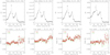 |
Fig. A.1. SYNOP1 single-slit observations on 2007-01-06 at 15:47 UT across an active region. Top row: peak DN along the slit, from the 90 s exposures. Bottom row: line widths (FWHM) from the 30 and 90 s exposures. The dashed line indicate the instrumental FWHM as estimated within the EIS software. |
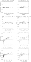 |
Fig. A.2. SYNOP1 single-slit observations on 2007-01-06 at 15:47 UT across an active region. From top to bottom: ratios of total counts in the 192 and 195 Å lines, as obtained by summing the pixel values and the Gaussian fit; ratio of the FWHM in the 195 versus the 192 Å lines; intensity ratio in the 195 Å line, between the 90 s and 30 s exposures; 192/195 Å and 192/193 Å line intensity ratios from the 90 s and 30 s exposures (in photons, dashed lines indicates expected values). |
The Fe XII intensity ratios become anomalous, as they vary with the intensity of the lines. The 192/195 Å ratio varies by
almost 40%. Blending cannot explain this behaviour: any blending in the two stronger lines would make the ratios vary in the opposite sense. The 195 Å line should increase its intensity in the active region, as the density-sensitive line in the self blend should become measurable. Instead, the intensity of the 195 Å line, compared to that of the 192 Å line, decreases. The important point is that the anomalous ratios are similar in both the 30 s and 90 s exposures. If the reason for the variation in the
ratio were due mainly to a non-linearity in the detector, the ratios should be different, as the 195 Å line is three times stronger in the 90 s exposure. We have seen this behaviour in all observations analysed.
Figure A.3 shows another SYNOP1 example, indicating very little variability in the Fe XII intensity ratios. However, the instrumental effect of the larger widths in the two stronger Fe XII lines is always present.
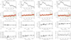 |
Fig. A.3. Quiet Sun SYNOP1 observations on 2007-06-09 at 06:12 UT. Top row: peak DN along the slit, from the 90 s exposures. Second row: line widths (FWHM) from the 30 and 90 s exposures. Note the larger scatter in the 30 s exposures, for low DN, below 200. Dashed lines: instrumental FWHM as in the EIS software. Third row: ratios of total counts in the 192 and 195 Å lines, as obtained by summing the pixel values and the Gaussian fit; 192/195 Å and 192/193 Å line intensity ratios from the 90 s exposures (in photons, dashed lines indicates expected values); Last row: effective FWHM in the three Fe XII lines, and the ratio of the 195 versus the 192 Å widths. |
Appendix B: A possible EIS saturation example
Figure B.1 shows one example where a saturation problem appears to be present. A portion of the EIS slit crossed an active region, around pixel coordinates 60–100, where counts peak. Panels a–b show the peak counts in the 192 and 195 Å lines with the 90 s exposures and the 195 Å line with the 30 s exposure.
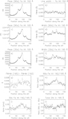 |
Fig. B.1. Active region SYNOP1 observations on 2006-12-29 at 11:15 UT. We note that the 195 Å line is saturated in one location, in the 90 s exposure. We also note the significant variation in the Fe XII intensity ratios. |
The 192 Å line does not show any significant variation in the width (panel b). On the other hand, the 195 Å line shows two strong increases in the width (panels d, f). These are the anomalous increases which are common in active region observations.
The second increase in the width around pixel 90 is more pronounced in the 90 s exposure (panel d), where the line reaches the EIS saturation limit, compared to the increase in the 30 s exposure. This is a different issue and is related to a saturation problem.
The overall difference in the widths of the two lines is around 4 mÅ (panel g) as we have seen in other cases. However, the difference increases up to 9 mÅ where the peak counts are (pixel 90).
Considering first the 30 s exposures, where both lines are far from the EIS saturation, we see in (panel i) that the ratio of the total intensities of the 192 and 195 Å lines is increased near the peak emission, from a value of about 0.3 to 0.35. Considering the 90 s exposures, the ratio is higher near the peak (panel h), an indication of a saturation problem. Indeed, considering the total intensity of the 195 Å line with the 90 s exposure, one would expect the ratios with the values obtained from the 30 s exposure to be 3, see panel l). However, the ratio consistently drops to lower values near the peak emission. This can only be an instrumental problem, unless the intensities changed only in those locations between the two exposures. The variation is not large though.
Appendix C: Our 2008-11-19 campaign
In Nov 2008, we ran a campaign to study the line width variations with the 2″ slit, scanning a small region of the Sun (60″ wide) with 60 s exposure times. We processed all observations, but found only one set to be useful.
Figure C.1 shows the variations of the line positions and FWHM as observed on 2008-11-19 with the EIS study GDZ_QS1_NS_60x512. The same solar region was observed with the bottom 512 and the top 512″ of the slit, successively. This is clear by looking at the variations of the intensities in the lines in the two parts of the CCD, divided by the vertical dashed line in Fig. C.1. This is important, and shows very little solar variability. We therefore expect the solar line widths to be the same. A small brightening was avoided, and 15 exposures were averaged. To further improve the signal, the spectra were rebinned by a factor of 3 along the slit. The variation of the line positions along the slit agrees very well with the values estimated by P. R. Young (shown as dashed lines), but the line widths still show some departures. It is worth noting very little change in the widths in the bottom part of the slit.
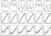 |
Fig. C.1. Top row: peak DN in a selection of SW lines, as a function of the position along the slit, for an average of 15 exposures of 60 s, with the 2″ slit on the quiet Sun, recorded on 2008-11-19 with the EIS study GDZ_QS1_NS_60x512. The dashed vertical line indicates the mid position of the 1024 slit. The bottom 512″ were observed by a raster starting at 11:38 UT, while the top 512″ were observed by a raster starting at 12:13 UT. Note the small temporal variation in the peaks of the lines. Middle row: line centroid positions; the dashed line indicates the estimated variation as available in the EIS software notes. Bottom row: FWHM in the lines, while the dashed line indicates the estimated variation as available in the EIS software notes. |
Appendix D: On-disk quiet Sun
We searched for EIS rasters with long exposures and with the full spectral range and the 1″ slit on the quiet Sun and found the first useful one was the study HPW001_FULLCCD_RAST_128x128_90S_SLIT1, with 90 s exposures and 128 slit positions. In spite of the long exposures, the strongest 195 Å line only reached a maximum of 5400 DN at line centre in a brightening near the limb, see Fig. D.1. Considering the dimmest regions, there is no obvious trend in the widths of the lines. However, the three lines have a consistently different width and the intensity ratios become anomalous above about 1500 DN in the brightest region, near the solar limb. The Fe XII intensity ratios are close to their expected values on-disk.
We searched for EIS rasters with long exposures, the full spectral range and the 2″ slit on the quiet Sun and found that one of the first ones was an Atlas_120x120_s2_40s with 40 s exposures on 2008-01-17. There is good signal in the Fe XII lines. Figure D.2 shows the main results. We see no trends in the widths. The counts in the lines are not very high. The Fe XII lines have however consistently different widths, as in the 1″ slit spectra. The line ratios are slightly below theory, indicating a change in the EIS calibration, in agreement with the results discussed in Del Zanna (2013a).
We searched for even longer exposures with the full spectral range and the 2″ slit and found the first useful one was an Atlas_120 taken on 2010-10-08. In spite of the long exposures, the strongest 195 Å line only had less then 3000 DN at line centre, see Fig. D.3. There is a small difference (3 mÅ) between the FWHM in the 192 and 195 Å lines. Above 2500 DN in the peak of the 195 Å line, some departure in the line ratio is visible. There is no obvious E-W variation of the line widths, as shown in the bottom of Fig. D.3. The 192/195 Å and 192/193 Å ratios are lower than expected in the dimmest regions, indicating instrumental degradation.
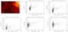 |
Fig. D.1. One of the earliest full-spectral EIS observations of the quiet Sun, with the 1″ slit on 2006-12-23. From left to right and top to bottom: peak DN in the Fe XII 195.1 Å line; FWHM of the three main Fe XII lines, as a function of their peak intensities (DN); intensity ratios of the lines, as a function of the peak intensities of the strongest line. The dashed lines indicate the expected values. |
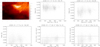 |
Fig. D.2. One of the earliest full spectral range quiet Sun on-disk observations with long exposures and with the 2″ slit (Atlas_120x120_s2_40s study), on 2008-01-17. |
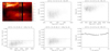 |
Fig. D.3. Quiet Sun on-disk observation with the 2″ slit and the Atlas_120 study, on 2010-10-08. |
Appendix E: Quiet Sun at the limb
Observations of the quiet Sun at the limb sometimes show strong anomalies, sometimes not. Figure E.1 shows an observation with the 1″ slit on 2007-03-11. There is little variation in the widths of the Fe XII lines, although the two stronger lines always have larger widths than the weaker line. The intensity ratios do not vary much.
We searched for QS observations with long exposures near the equator, and found that the first useful one was an Atlas_120 taken on 2011-01-04 at 12:59 UT. It observed up to about 100″ above the limb. The strongest 195 Å line was nearly saturated near the limb, see Fig. E.2. The 192 Å and 195 Å lines indicate a small decrease in the line width off-limb. The 192/195 Å and 192/193 Å ratios are lower than expected in the dimmest regions, indicating an instrumental degradation. The ratios show the anomalous effect in the brightest regions, most likely due to opacity.
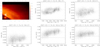 |
Fig. E.1. QS off-limb observation with the 1″ slit, 90 s exposures on 2007-03-11. |
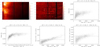 |
Fig. E.2. Quiet Sun observation at the limb with the 2″ slit and an Atlas_120 taken on 2011-01-04 at 12:59 UT. |
Appendix F: 2018 observations – Quiet Sun – bottom of the slit
We obtained QS rasters with the bottom of the slit, pointed near Sun centre, to use as a reference, mostly to see if there were any E-W variations in the line widths in this part of the slit. The signal was very low, so only the strongest 195 Å line was usable. Figure F.1 (top) shows the image of the width of the line, while Fig. F.1 (bottom) shows the averaged values along the E-W direction, indicating no obvious variations.
 |
Fig. F.1. An observation of the FWHM of the strongest 195 Å line, in the bottom of the EIS 2″ slit on the Quiet Sun near Sun centre, indicating no obvious E-W variations. |
Appendix G: The off-limb QS observations out to 1.5 R⊙ on 2007-05-08
Figures G.1 and G.2 show a sample of results from the analysis of the off-limb observation on 2007-05-8. The presence of the active region at the limb somewhat affected the nearby corona, which can be seen by a small increase in the ionisation temperatures, compared to the values we measured two days later. The observed line widths are also nearly constant, with a small increase with radial distance.
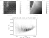 |
Fig. G.1. Selected results from the Hinode EIS off-limb observation on 2007-05-8 at 13:51 UT. From top to bottom: image of the FWHM and peak DN in the Fe XII 195.1 Å line; scatter plot of the FWHM as a function of peak intensity. |
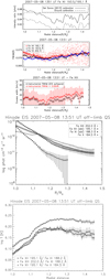 |
Fig. G.2. From top to bottom: measured intensity ratio of the Fe XII 193.5 versus 195.1 Å lines on 2007-05-8, as function of radial distance in the QS sector; observed FWHM of the main three lines, from averaged spectra along the radial QS sector, with the pixel-by-pixel FWHM of the 195.1 Å line (points); excess width from the Fe XIII line; radiances of selected lines along the radial QS sector; isothermal temperatures along the radial QS sector. |
The excess widths were estimated from the Fe XIII line, assuming the temperatures from the Fe XII/Fe X ratio, and adding a (small) uncertainty of 3 mÅ in the observed widths. The boxes show the results with the instrumental width as in the EIS software. The triangles assume a constant instrumental width of 64 ± 2 mÅ.
2018 July QS off-limb observations out to 1.5 R⊙
As most of the 2007 observations were affected somewhat by the presence of the active region, we have recently obtained new observations with the special EIS study gdz_off_limb1_60 in July 2018, when the Sun was very quiet. The pointing was similar to the 2007 observations, in the south-west. As the EIS instrument has degraded and the solar signal is lower, these observations are of less quality than the previous ones. Figure G.3 shows the widths obtained from the two main lines, obtained from a radial sector. As in the 2007 observations, a small decrease around the limb is visible. However, the variation is not significant considering the various uncertainties we have described above. The small increase above 1.2 R⊙ is also most probably not real, as the lines were very weak.
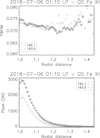 |
Fig. G.3. QS off-limb observations out to 1.5 R⊙, on 2018-07-06. Top plot: variation of the FWHM in the two strongest Fe XII lines, as a function of distance along a radial sector. Bottom plot: peak counts in the lines. |
Appendix H: AR observations on-disk
We searched for observations on active regions with the full spectral range and the 1″ slit. The earliest useful one was the study HPW001_FULLCCD_RAST_128x128_90S_SLIT1 with with 90 s exposures and 128 slit positions. The strongest lines are saturated in the brightest regions. We removed the pixels where the lines have more than 12 000 DN in their peak intensity. The range of peak values considered for the 195 Å line goes from 1000 to 12 000 DN, as shown in Fig. H.1. The widths of the lines tend to be narrower in the regions with lowest intensities. There is a small difference between the FWHM in the lines. The 192/195 Å and 192/193 Å ratios are slightly lower than theory in the dimmest regions, and show significant instrumental effects.
We searched for observations on active regions with the full spectral range and the 2″ slit and found the first useful one was a study with 40 s exposures, taken on 2007-05-21 at 07:27 UT (see Fig. H.2). This observation was studied by Del Zanna & Ishikawa (2009) as it contained a small flare. The strongest lines are saturated in the brightest regions. We removed the pixels where the lines have more than 12 000 DN in their peak intensity. There is no obvious variation with line width and intensity. However, the 195 Å line consistently has a larger width. The 192/195 Å and 192/193 Å ratios are close to their expected values in the dimmest regions, but show significant opacity effects in the brightest regions.
For active region observations, assuming a FWHM of 0.03 Å, a typical averaged density of 2 × 109 cm−3, “coronal” abundances (increased by 3.2 over photospheric, see Del Zanna & Mason 2018), Nl/N(Fe XII) = 0.75, an opacity at line centre of one would require a path length ΔS = 4 × 10⁴ Km, which is a large but not unreasonable path length.
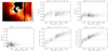 |
Fig. H.1. Active region on-disk observation on 2006-12-25 with the 1″ slit, with the HPW001_FULLCCD_RAST_128x128_90S_SLIT1 study. |
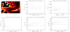 |
Fig. H.2. Active region on-disk observation on 2007-05-21 with the 2″ slit. |
All Figures
|
Fig. 1. Top row: peak DN in a selection of SW lines, as function of slit position, for 160 s exposure with 2″ slit on the quiet Sun, recorded on 2006-10-28. The dashed vertical line indicates the mid position of the 1024 slit. Middle row: line centroid positions (Å); the dashed line indicates the estimated variation as available in the EIS software notes. Bottom row: FWHM (Å) in the lines, while the dashed line indicates the estimated variation as available in the EIS software notes. The bottom axis is the position along the slit, from bottom (pixel 0) to the top (pixel 1023). |
| In the text | |
|
Fig. 2. Differences in the FWHM of the three main Fe XII lines, as a function of the position along the slit, for the same observation in Fig. 1. |
| In the text | |
|
Fig. 3. Monochromatic images (negative) in a few spectral lines, obtained on 2007-05-10 with Hinode EIS. The radial sector used to obtain averaged spectra in the quiet corona as a function of radial distance is indicated. |
| In the text | |
|
Fig. 4. Selected results from the Hinode EIS off-limb observation on 2007-05-10 at 10:21 UT. Top: images of the peak intensity (DN) and FWHM (mÅ) in the Fe XII 195.1 Å line. Bottom: scatter plot of the FWHM (Å) as a function of peak intensity. |
| In the text | |
|
Fig. 5. FWHM of the Fe XII 195.1, 193.5 Å and Fe XIII 202 Å lines, obtained from averaged spectra along the radial QS sector shown in Fig. 3. The points are the pixel-by-pixel FWHM of the 195.1 Å line. |
| In the text | |
|
Fig. 6. Excess widths from the Fe XIII 202 Å line as a function of radial distance, obtained from the radial QS sector shown in Fig. 3, assuming two different instrumental widths. |
| In the text | |
|
Fig. 7. Left: off-limb variations of the FWHM in the three Fe XII lines, obtained from a “quiet” region 30″ wide observed on 2007-12-17 (see Gupta 2017); variations of the peak line intensities (DN). Right: variations of the calibrated intensity line ratios, with the expected values shown as dashed lines. |
| In the text | |
|
Fig. 8. Off-limb variations of the FWHM and peak line intensities for the strongest Fe XIII and Fe XV lines along the same “quiet” region 30″ wide as observed on 2007-12-17 and as on Fig. 7 (top and middle plot). Bottom plot: excess width in the Fe XIII line. |
| In the text | |
|
Fig. 9. Quiet Sun east limb observation on 2013-02-14 at 09:49 UT. Top images: peak intensity of the 195 Å line (DN), the observed FWHM (Å) of the 192 Å line, and the intensity ratio of the 192 and 195 Å lines. The coordinates are the pixel positions. The arrows indicate two regions, off-limb (OL) and on-disk (OD) chosen for further studies. Lower plots: scatter plots of the FWHM in the 192 and 195 Å lines, as a function of their peak intensity, and the intensity ratio of the 192/195 Å lines. The dashed line indicate the expected value. |
| In the text | |
|
Fig. 10. Emissivity ratio plots for the main Fe XII lines in the on-disk (top) and off-limb (bottom) regions indicated in Fig. 9. The calibrated intensities (in photons cm−2 s−1 arcsec−2) are shown in the plots (Iob). |
| In the text | |
|
Fig. 11. DEM distribution for the off-limb region indicated in Fig. 9. The points indicate the ratio of the predicted versus observed radiance, multiplied by the DEM value at the temperature of maximum emissivity in each line. |
| In the text | |
|
Fig. 12. Top: logarithmically-scaled intensity of the Fe XII 195 Å line along 304″ of the 1″ slit, across AR loops observed on 2007 May 6, as in Fig. 12 of Young et al. (2009). Middle: intensity ratios of the Fe XII lines, using the ground calibration. Bottom: intensity ratio of the Fe XII 192 versus 195 Å lines as a function of the peak intensity in the stronger line, and for two different radiometric calibrations. |
| In the text | |
|
Fig. 13. Top: peak intensity (DN) and FWHM (km s−1) of the 195 Å line, with pixels above 12 000 blanked. Bottom: 192/195 Å intensity ratio (phot), and difference between the FWHM of the 195 and 192 Å lines (km s−1). Two regions selected for further analysis, on a moss and a quiet region (QR) within the active region are shown. |
| In the text | |
|
Fig. 14. Emissivity ratio plots for the main Fe XII lines in the moss and quiet regions indicated in Fig. 13. The calibrated intensities (in photons cm−2 s−1 arcsec−2) are shown in the plots (Iob). |
| In the text | |
|
Fig. A.1. SYNOP1 single-slit observations on 2007-01-06 at 15:47 UT across an active region. Top row: peak DN along the slit, from the 90 s exposures. Bottom row: line widths (FWHM) from the 30 and 90 s exposures. The dashed line indicate the instrumental FWHM as estimated within the EIS software. |
| In the text | |
|
Fig. A.2. SYNOP1 single-slit observations on 2007-01-06 at 15:47 UT across an active region. From top to bottom: ratios of total counts in the 192 and 195 Å lines, as obtained by summing the pixel values and the Gaussian fit; ratio of the FWHM in the 195 versus the 192 Å lines; intensity ratio in the 195 Å line, between the 90 s and 30 s exposures; 192/195 Å and 192/193 Å line intensity ratios from the 90 s and 30 s exposures (in photons, dashed lines indicates expected values). |
| In the text | |
|
Fig. A.3. Quiet Sun SYNOP1 observations on 2007-06-09 at 06:12 UT. Top row: peak DN along the slit, from the 90 s exposures. Second row: line widths (FWHM) from the 30 and 90 s exposures. Note the larger scatter in the 30 s exposures, for low DN, below 200. Dashed lines: instrumental FWHM as in the EIS software. Third row: ratios of total counts in the 192 and 195 Å lines, as obtained by summing the pixel values and the Gaussian fit; 192/195 Å and 192/193 Å line intensity ratios from the 90 s exposures (in photons, dashed lines indicates expected values); Last row: effective FWHM in the three Fe XII lines, and the ratio of the 195 versus the 192 Å widths. |
| In the text | |
|
Fig. B.1. Active region SYNOP1 observations on 2006-12-29 at 11:15 UT. We note that the 195 Å line is saturated in one location, in the 90 s exposure. We also note the significant variation in the Fe XII intensity ratios. |
| In the text | |
|
Fig. C.1. Top row: peak DN in a selection of SW lines, as a function of the position along the slit, for an average of 15 exposures of 60 s, with the 2″ slit on the quiet Sun, recorded on 2008-11-19 with the EIS study GDZ_QS1_NS_60x512. The dashed vertical line indicates the mid position of the 1024 slit. The bottom 512″ were observed by a raster starting at 11:38 UT, while the top 512″ were observed by a raster starting at 12:13 UT. Note the small temporal variation in the peaks of the lines. Middle row: line centroid positions; the dashed line indicates the estimated variation as available in the EIS software notes. Bottom row: FWHM in the lines, while the dashed line indicates the estimated variation as available in the EIS software notes. |
| In the text | |
|
Fig. D.1. One of the earliest full-spectral EIS observations of the quiet Sun, with the 1″ slit on 2006-12-23. From left to right and top to bottom: peak DN in the Fe XII 195.1 Å line; FWHM of the three main Fe XII lines, as a function of their peak intensities (DN); intensity ratios of the lines, as a function of the peak intensities of the strongest line. The dashed lines indicate the expected values. |
| In the text | |
|
Fig. D.2. One of the earliest full spectral range quiet Sun on-disk observations with long exposures and with the 2″ slit (Atlas_120x120_s2_40s study), on 2008-01-17. |
| In the text | |
|
Fig. D.3. Quiet Sun on-disk observation with the 2″ slit and the Atlas_120 study, on 2010-10-08. |
| In the text | |
|
Fig. E.1. QS off-limb observation with the 1″ slit, 90 s exposures on 2007-03-11. |
| In the text | |
|
Fig. E.2. Quiet Sun observation at the limb with the 2″ slit and an Atlas_120 taken on 2011-01-04 at 12:59 UT. |
| In the text | |
|
Fig. F.1. An observation of the FWHM of the strongest 195 Å line, in the bottom of the EIS 2″ slit on the Quiet Sun near Sun centre, indicating no obvious E-W variations. |
| In the text | |
|
Fig. G.1. Selected results from the Hinode EIS off-limb observation on 2007-05-8 at 13:51 UT. From top to bottom: image of the FWHM and peak DN in the Fe XII 195.1 Å line; scatter plot of the FWHM as a function of peak intensity. |
| In the text | |
|
Fig. G.2. From top to bottom: measured intensity ratio of the Fe XII 193.5 versus 195.1 Å lines on 2007-05-8, as function of radial distance in the QS sector; observed FWHM of the main three lines, from averaged spectra along the radial QS sector, with the pixel-by-pixel FWHM of the 195.1 Å line (points); excess width from the Fe XIII line; radiances of selected lines along the radial QS sector; isothermal temperatures along the radial QS sector. |
| In the text | |
|
Fig. G.3. QS off-limb observations out to 1.5 R⊙, on 2018-07-06. Top plot: variation of the FWHM in the two strongest Fe XII lines, as a function of distance along a radial sector. Bottom plot: peak counts in the lines. |
| In the text | |
|
Fig. H.1. Active region on-disk observation on 2006-12-25 with the 1″ slit, with the HPW001_FULLCCD_RAST_128x128_90S_SLIT1 study. |
| In the text | |
|
Fig. H.2. Active region on-disk observation on 2007-05-21 with the 2″ slit. |
| In the text | |
Current usage metrics show cumulative count of Article Views (full-text article views including HTML views, PDF and ePub downloads, according to the available data) and Abstracts Views on Vision4Press platform.
Data correspond to usage on the plateform after 2015. The current usage metrics is available 48-96 hours after online publication and is updated daily on week days.
Initial download of the metrics may take a while.