| Issue |
A&A
Volume 630, October 2019
|
|
|---|---|---|
| Article Number | A73 | |
| Number of page(s) | 14 | |
| Section | Interstellar and circumstellar matter | |
| DOI | https://doi.org/10.1051/0004-6361/201935920 | |
| Published online | 24 September 2019 | |
The physical and chemical structure of Sagittarius B2
V. Non-thermal emission in the envelope of Sgr B2
1
I. Physikalisches Institut, Universität zu Köln,
Zülpicher Str. 77,
50937
Köln,
Germany
e-mail: meng@ph1.uni-koeln.de
2
INAF – Osservatorio Astrofisico di Arcetri,
Largo Enrico Fermi 5,
50125
Firenze,
Italy
3
Laboratoire Univers et Particules de Montpellier, UMR 5299 du CNRS, Université de Montpellier,
place E. Bataillon, cc072,
34095
Montpellier,
France
4
Jansky Fellow of the National Radio Astronomy Observatory,
1003 Lopezville Rd.,
Socorro,
NM
87801,
USA
5
Max Planck Institute for Extraterrestrial Physics,
Giessenbachstrasse 1,
85748
Garching,
Germany
6
Agnes Scott College,
141 E. College Ave.,
Decatur,
GA
30030,
USA
Received:
20
May
2019
Accepted:
15
August
2019
Context. The giant molecular cloud Sagittarius B2 (hereafter Sgr B2) is the most massive region with ongoing high-mass star formation in the Galaxy. In the southern region of the 40-pc large envelope of Sgr B2, we encounter the Sgr B2(DS) region, which hosts more than 60 high-mass protostellar cores distributed in an arc shape around an extended H II region. Hints of non-thermal emission have been found in the H II region associated with Sgr B2(DS).
Aims. We seek to characterize the spatial structure and the spectral energy distribution of the radio continuum emission in Sgr B2(DS). We aim to disentangle the contribution from the thermal and non-thermal radiation, as well as to study the origin of the non-thermal radiation.
Methods. We used the Very Large Array in its CnB and D configurations, and in the frequency bands C (4–8 GHz) and X (8–12 GHz) to observe the whole Sgr B2 complex. Continuum and radio recombination line maps are obtained.
Results. We detect radio continuum emission in Sgr B2(DS) in a bubble-shaped structure. From 4 to 12 GHz, we derive a spectral index between − 1.2 and − 0.4, indicating the presence of non-thermal emission. We decomposed the contribution from thermal and non-thermal emission, and find that the thermal component is clumpy and more concentrated, while the non-thermal component is more extended and diffuse. The radio recombination lines in the region are found to be not in local thermodynamic equilibrium but stimulated by the non-thermal emission.
Conclusions. Sgr B2(DS) shows a mixture of thermal and non-thermal emission at radio wavelengths. The thermal free–free emission is likely tracing an H II region ionized by an O 7 star, while the non-thermal emission can be generated by relativistic electrons created through first-order Fermi acceleration. We have developed a simple model of the Sgr B2(DS) region and found that first-order Fermi acceleration can reproduce the observed flux density and spectral index.
Key words: stars: formation / ISM: individual objects: Sgr B2 / radio continuum: ISM / radio lines: ISM / ISM: clouds / stars: massive
© ESO 2019
1 Introduction
The giant molecular cloud Sagittarius B2 (hereafter Sgr B2) is the most massive (~107 M⊙, see e.g., Goldsmith et al. 1990) region with ongoing high-mass star formation in the Galaxy, and has a higher density (>105 cm−3) and dust temperature (~50–70 K) compared to other star forming regions in the Galactic plane (see e.g., Ginsburg et al. 2016; Schmiedeke et al. 2016; Sánchez-Monge et al. 2017). Sgr B2 is located at a distance of 8.34 ± 0.16 kpc, at only 100 pc in projection from the Galactic center (Reid et al. 2014)1. In the central ~2 pc, there are the two well-known hot cores Sgr B2(N) and Sgr B2(M) (see e.g., Schmiedeke et al. 2016; Sánchez-Monge et al. 2017), which contain at least 70 high-mass stars (see e.g., Gaume et al. 1995; De Pree et al. 1998, 2014). A larger envelope surrounding the two hot cores has a radius of 20 pc and contains more than 99% of the total mass of Sgr B2 (Schmiedeke et al. 2016, see also their Fig. 1 for a sketch of this region). The relatively high temperatures, densities, and pressure, as well as its proximity to the Galactic center make Sgr B2 a good target for studying high-mass star formation in extreme environments. With this in mind, we have started a project to characterize the physical and chemical properties via observations and modeling (Schmiedeke et al. 2016; Sánchez-Monge et al. 2017; Pols et al. 2018; Schwörer et al. 2019). The current work is the fifth paper in the series. While the first observational studies focused on the two central hot cores Sgr B2(N) and Sgr B2(M), in this work we investigate the physical properties of the envelope they are embedded in.
Previous studies of Sgr B2 suggest the presence of star forming activities throughout the envelope and not only in the central regions Sgr B2(N) and (M). Martín-Pintado et al. (1999) report the presence of filament-, arc- and shell-shaped dense gas likely produced by stellar feedback. Recent observations with ALMA at 3 mm revealed more than 200 high-mass protostellar cores distributed throughout the envelope (Ginsburg et al. 2018). A remarkable feature is the presence of about 60 dense cores in the southern region, following an arc-shape distribution. This group of cores is spatially coincident with the arc-shaped feature detected in NH3 by Martín-Pintado et al. (1999), which is referred to as Deep South (DS) by Ginsburg et al. (2018). At the position of Sgr B2(DS), Mehringer et al. (1993) report the detection of radio continuum and radio recombination line (RRL) emission (see also LaRosa et al. 2000; Law et al. 2008). Such continuum emission at radio wavelengths along with RRLs is usually related to thermal ionized gas from H II regions (e.g., Kurtz 2002, 2005). However, along with the thermal emission detected in previous studies, non-thermal emission, has also been found in Sgr B2 due to relativistic electrons (LaRosa et al. 2005; Hollis et al. 2007; Protheroe et al. 2008; Jones et al. 2011). Yusef-Zadeh et al. (2007a, 2013, 2016) studied the presence of non-thermal emission in the Galactic Center region including Sgr B2. Particularly, observations at 255 MHz, 327 MHz, and 1.4 GHz (Yusef-Zadeh et al. 2007b) revealed non-thermal emission in Sgr B2(M). The thermal andnon-thermal contribution to the radio continuum emission can be distinguished by their spectral energy distribution (SED). The SEDs of both thermal and non-thermal emission can be described by power-laws Sν ∝να, where α is the so-called spectral index, whichvaries from − 0.1 to +2 for thermal emission (see e.g., Sánchez-Monge et al. 2013) and becomes significantly negative for non-thermal emission (e.g., α = −0.8, see Platania et al. 1998).
In this paper, we present Very Large Array (VLA) observations of the whole Sgr B2 region in the frequency regime 4–12 GHz, with configurations BnC and D. Thus, this study focuses on spatial scales from 0.2–10 pc. The higher sensitivity and resolution compared to previous studies allow us to study in detail the presence and properties of radio-continuum sources, both thermal and non-thermal, throughout Sgr B2. Although the observations cover the whole envelope of Sgr B2, we pay special attention to Sgr B2(DS). In Sect. 2 we describe the observations as well as the data reduction process. Section 3 shows the results, and the study of the spectral index. In Sect. 4 we aim at decomposing the thermal and non-thermal components dominating the emission at radio wavelengths, while in Sect. 5 we discuss on the origin of the non-thermal emission. Finally, we summarize our study in Sect. 6.
2 Observations and data reduction
We used the VLA in its CnB and D configurations to observe the entire Sgr B2 complex in the frequency bands C (4–8 GHz) and X (8–12 GHz). The observations with the CnB configuration were conducted on May 3 and 5, 2016 (project 16A-195). On February 22and 23, 2017, the D configuration was employed for the observations (project 17B-063). The continuum emission was observed by combining a total of 64 spectral windows with a bandwidth of 128 MHz each. Alongside the continuum observations, high-resolution spectral windows were used for line observations. Eighteen RRLs in the frequency range from 4 to 12 GHz were observed with a spectral resolution between 31.25 and 62.5 kHz (1–2 km s−1). In Table 1, we list the rest frequencies of the 18 RRLs. We used the mosaic mode to cover the whole extent of Sgr B2 (~ 20′ × 20′). A total of 10 and 18 pointings, with primary beam sizes of 7.5′ and 4.5′ for the C and X bands, respectively, were used. The quasar 3C286 was used as a flux and bandpass calibrator. The SED of 3C286 from 0.5 to 50 GHz was measured by Perley & Butler (2013), with a flux of 5.059± 0.021 Jy at 8.435 GHz and a spectral index of − 0.46. The quasar J1820-2528, the flux of which is 1.3 Jy in the C and X bands, was used as phase calibrator. The calibration was done using the standard VLA pipelines provided by the NRAO2.
Calibration and imaging were done in Common Astronomy Software Applications (CASA) 4.7.2 (McMullin et al. 2007). The calibrated measurement sets of the CnB and D array data were concatenated to improve the uv sampling. Self-calibration was performed to reduce imaging artifacts and improve the final sensitivity of the image. Three loops of phase-only self-calibration were conducted, with solution time intervals of two seconds, equal to theintegration time of the observations. The self-calibrated measurement sets were used for imaging. All the pointings of the mosaic in each band were primary beam corrected and the mosaic was imaged using the CASA task tclean. With a robust factor of 0.5, the images of the C and X bands have synthesized beams of 2.7′′ × 2.5′′, with a position angle (PA) of − 82° and 1.8′′ × 1.5′′ (PA = 76°), respectively. The PA is defined positive north to east. Under such resolutions, the root mean square (RMS) noise of the C and X band images are 0.4 and 0.2 mJy beam−1 respectively. This RMS noise is limited by dynamic range effects due to the bright emission in the region. We achieve a dynamic range of about 4000 and 2000 for the X- and C-band images, respectively. To investigate the SED over the whole 4–12 GHz range, the measurement sets of the C and X bands were divided into 12 frequency ranges. Thus, 12 images from 4 to 12 GHz were obtained. The uv coverage was restricted to 0.6–50 kλ for each frequency range to ensure that every image is sensitive to same spatial scales. The 12 images are convolved to a final circular Gaussian beam of 4′′. In addition to the continuum emission, we also imaged the 18 RRLs. In order to increase the signal-to-noise ratio (S/N), we stacked the neighboring RRLs to produce a final set of four stacked RRLs (see Table 1 for details). All the RRL images were resampled to a common spectral resolution of 2.5 km s−1. Finally, and with the aim of compensating for the low sensitivity (3 mJy beam−1 per 2.5-km s−1 channel), the images of the four stacked RRLs are smoothed to a resolution of 8′′, resulting in a final sensitivity of 1 mJy beam−1 per 2.5-km s−1 channel.
Observed and stacked RRLs.
3 Results
In this section we discuss the distribution of the radio continuum emission in the Sgr B2 region, characterize the spectral index, and study the RRL emission. We pay special attention to the Sgr B2(DS) region.
3.1 Ionized gas in Sgr B2(DS)
The images of the Sgr B2 region in the C and X bands are shown in Fig. 1. Some relevant objects such as the regions Sgr B2(N), (M) and (S) are indicated, as well as source V and the H II region AA (see Mehringer et al. 1993). The DS region is the main focus of this article. It appears as a bubble-like structure with an outer-diameter of ~ 1.5 pc. The thickness of the bubble edge is ~ 0.3 pc, with the eastern part being stronger than the western region of the bubble, in both X and C-band images. Filaments and arcs are found along the edge of the bubble, while the emission towards the center is just at the RMS noise level.
The radio continuum emission in DS is spatially connected to the high-mass dust cores revealed by previous ALMA observationsat millimeter wavelengths (Ginsburg et al. 2018). As shown in Fig. 2, more than 60 dust cores are located at the outskirts of the bubble-like structure, with a larger population of dense cores to the east.
3.2 Spectral index analysis
The C and X band data, from 4 to 12 GHz, are divided into 12 tomographic maps and convolved to a common angular resolution of 4′′. To ensure that each of the 12 channel maps is sensitive to similar spatial scales, we have set the uv limit to the common range 0.6–50 kλ. Moreover, we have checked that large-scale background emission does not affect the spectral analysis. For this, we have inspected intensity profiles of the 12 channel maps, and found the background emission to be zero (see Appendix A and Fig. A.1). In Fig. 3, we show the portion of the map corresponding to Sgr B2(DS). The intensity decreases significantly from 4 to 12 GHz. We analyzed the SED of the radio emission in DS by fitting a power law to the 12 tomographic maps. We define the variation of flux with frequency as Sν ∝ να, where Sν denotes the flux density, ν stands for frequency, and α is the spectral index. The power-law fitting is conducted pixel by pixel for the whole map. For each pixel, the spectral index is fit only if the emission in all the 12 tomographic maps is above 3σ, otherwise the pixel is masked. To avoid effects of possible artifacts, the fitting minimizes a loss function  , where z is the square of the difference between the fit power-law function and the observed intensity in the 12 frequency ranges. The uncertainty of α is obtained from the corresponding diagonal element of the covariance matrix of the fitting.
The fit spectral index map of the whole Sgr B2 region, as well as the map of uncertainty of α are shown in Fig. 4. The hot cores N, M, as well as other sources in the whole Sgr B2 region, except DS, show spectral indices between − 0.01 and 2, which are consistent with thermal emission from H II regions. The central parts in N and M have spectral index values greater than 1, which indicates that the emission is optically thick. At the edges of these hot cores we determine flatter SEDs (e.g., α = −0.1), suggesting that the centimeter emission at the edges of these H II regions becomes optically thin.
In contrast to most regions in Sgr B2, the major part of DS shows negative spectral index values (see also Fig. 5). We have highlighted the SED of six selected positions in the DS region and shown them in Fig. 5. Source AA is included as reference for the spectral index, since it is a known H II region with optically thin free–free emission (Mehringer et al. 1993). As displayed in Fig. 5, source AA has α = 0.01 ± 0.06, consistent with optically thin free–free emission. The other five spots have negative spectral indices, ranging from − 0.4 to − 1.2. Such values indicate the existence of non-thermal emission in DS. As shown in the map, the distribution of the non-thermal emission extends to more than 1 pc and forms arc structures.
With the goal of confirming the spectral index values derived from the VLA data, we have used data from the Giant Metrewave Radio Telescope (GMRT) at 350 MHz (Meng et al., in prep.). We have recently observed a large region in the Galactic center around SgrB2, reaching an angular resolution of 12.2′′ × 11.7′′ (PA = 57°) and an rms noise level of 0.05 mJy beam−1. In Appendix B we compare the flux of DS at 350 MHz with the VLA data. The spectral index between 350 MHz and 4 GHz (see Fig. B.1) is consistent with the VLA spectral index map shown in Fig. 4, confirming the presence of non-thermal emission in DS.
3.3 Radio recombination line emission
In addition to the continuum emission, we also observed RRLs in the whole Sgr B2 region. Due to the low sensitivity of these maps, we have smoothed the images to 8′′. At this resolution we are still capable to resolve the structure of the DS region. On the smoothed maps, Gaussian fitting was conducted and peak intensity, centroid velocity, line width and integrated intensity were obtained for all the four stacked RRLs (see Fig. C.1).
The integrated intensity maps of the four RRLs show distinct spatial distribution. At 4.4 GHz, the emission appears relatively diffuse, while at 6.8 GHz, different clumpy structures are visible. At 8.9 GHz the northern part of DS is brighter, while at 10.5 GHz, the southern part of DS has more emission. Such a variation is inconsistent with a simple thermal RRL scenario but suggests the presence of other excitation mechanisms, which will be discussed in Sect. 4.2. The velocity maps of the four RRLs are in agreement for the four images. The eastern lobe of the bubble shows a velocity gradient ranging from velocities about 70 km s−1 in the center down to 55 km s−1 in the outer edge. As shown in the line width maps, the RRLs are typically broad, with values above 30 km s−1, significantly exceeding the thermal broadening of RRLs in H II regions with electron temperatures Te = 104 K (Δv ≈ 20 km s−1). Notably, the line width at the eastern edge of the bubble reaches more than 40 km s−1. The velocity difference between the eastern edge of DS and the center, together with the increase of line width at the eastern edge, suggests a possible interaction between the expanding H II region and its surrounding material.
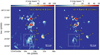 |
Fig. 1 Continuum images of Sgr B2 in C (panel a) and X (panel b) bands. Relevant regions are marked with their names (see Mehringer et al. 1993). The dashed boxes mark the region of DS. The synthesized beam of the C and X images are 2.7′′ × 2.5′′ and 1.82′′ × 1.53′′, respectively |
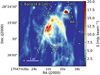 |
Fig. 2 C band (4–8 GHz) continuum emission map of Sgr B2(DS). The circles mark the positions of the high-mass protostellar cores identified by Ginsburg et al. (2018). The synthesized beam is shown as a yellow ellipse at the bottom left corner. |
4 Thermal and non-thermal components in Sgr B2(DS)
The power-law fitting of the continuum emission in Sgr B2(DS) results in a spectral index α that varies from − 1.2 to − 0.1. The observed range of values of α implies that the centimeter continuum emission in DS is a mixture of thermal and non-thermal contributions. In this section, we dissect the thermal and non-thermal components in the continuum emission and also analyze the properties of the RRL emission.
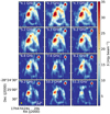 |
Fig. 3 Channel maps of the Sgr B2(DS) region. All the 12 maps have been produced considering the same uv range limited to 0.6–50 kλ, and have been convolved to a circular beam of 4′′. The synthesized beam is shown as a yellow circle in the bottom left panel. |
4.1 Disentangling the thermal and non-thermal components
In the following we present two different approaches to disentangle the contributions of the thermal and non-thermal emission in order to better characterize their origin in Sect. 5. The two methods are extrapolating high-frequency emission and fitting the SED with fixed spectral indices.
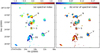 |
Fig. 4 Spectral index (α, panel a) andits uncertainty, (panel b) throughout the whole Sgr B2 region. The regions marked in both panels correspond to those regions also labeled in Fig. 1. See Sect. 3.2 for details in the calculation of the spectral index. |
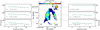 |
Fig. 5 Spectral index of DS. Six spots are taken as examples to show the fitting of SED and the fit spectral index (α). The contours are where the flux density at 4 GHz is 10 mJ beam−1. The angular resolution is 4′′ × 4′′, and the beam is shown in the lower left corner. |
4.1.1 Extrapolating high-frequency emission
Thermal emission at radio wavelengths is characterized by a relation in which the intensity increases with or is independent of the frequency. On the contrary, the non-thermal emission is characterized by the intensity decreasing with frequency. This suggests that the emission at higher frequencies (corresponding to 11.2 GHz in our dataset) is likely to be dominated by the thermal component, while the emission at lower frequencies (corresponding to 4 GHz) is dominated by the non-thermal component. In our first approach, we assume that the emission at the highest frequency in our data is dominated by pure thermal (free–free) emission.
The total flux of DS at 11.2 GHz is 0.5 Jy within a diameter of ~ 36′′, corresponding to a brightness temperature of 14 K. For a typical H II region temperature of 5 × 10³–104 K, the optical depth τ ranges from 1.4 × 10⁻³ to 2.8 × 10⁻³. Therefore, the free–free emission of DS is optically thin. We use the typical spectral index α = −0.1 of optically thin free–free emission to extrapolate the 11.2 GHz flux density to 4 GHz. The extrapolated thermal component is subtracted from the observed flux density at 4 GHz to get a pure non-thermal component. In Fig. 6 we show the derived thermal and non-thermal components at 4 GHz. The non-thermal emission appears more widespread, while the thermal component appears concentrated in different clumps located along the edge of the bubble. As expected, the H II region AA has strong thermal emission, while at 4 GHz, the contribution from the non-thermal component drops below the RMS level. Only in the southeastern region, connecting source AA with the bubble-like structure of DS, we find some presence of a possible contribution of non-thermal emission.
The total observed flux at 4 GHz (within the circle highlighted in Fig. 6) is ~ 1.5 Jy, for which we determine that ~60% has a non-thermal origin. We note that since we have assumed that the emission at 11.2 GHz is purely thermal, the contribution of thermal emission at 4 GHz is most likely overestimated and therefore, the non-thermal contribution may be underestimated.
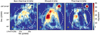 |
Fig. 6 Spatial distribution of synchrotron (or non-thermal, left panel), mixed (central panel, corresponding to observed image) and free–free (or thermal, right panel) components of DS at 4 GHz as derived from method described in Sect. 4.1.1. The thermal emission map is extrapolated from 12 GHz assuming that at this frequency the emission is originated by a thermal component with a spectral index α = −0.1. The non-thermal emission is obtained by subtracting the extrapolated thermal emission from the mixed emission. The contours are the same as in Fig. 5. All panels have a circular beam of 4′′ (shown in the bottom left corner of each panel). The dashed circles indicate the region in which we calculate the flux density of DS (see Sect. 4.1). |
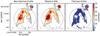 |
Fig. 7 Spatial distribution of the synchrotron (left panel), mixed (central panel) and free–free (right panel) components of DS at 4 GHz. All the three images are obtained after fitting the observed SED with the sum of two power-law functions: Sth (ν) ∝ ν−0.1 and Snt (ν) ∝ ν−0.7 for the thermal and non-thermal components, respectively (see details in Sect. 4.1.2). The contours are the same as in Fig. 5. All panels have a circular beam of 4′′ (shown in the bottom left corner of each panel). The dashed circles indicate the region in which we calculated the flux density of DS (see Sect. 4.1). |
4.1.2 Fitting the SED with fixed spectral indices
In a second approach, we aim at simultaneously determining the contribution of thermal and non-thermal emission. For this, we fit the SED covering the whole range from 4 to 12 GHz with two power-law functions describing each component. For the thermal component, the power-law is Sth(ν) ∝ ν−0.1, assuming that the emission is optically thin free–free. For the non-thermal component, we use Snt (ν) ∝ ν−0.7 (see Hollis et al. 2003; Protheroe et al. 2008; Jones et al. 2011). We fit the observed SED with a linear superposition of these two power-law functions and get the contribution of each component at different frequencies.
As shown in Fig. 7, at 4 GHz, the spatial distribution of the non-thermal component is more widespread compared tothe thermal component which is mainly concentrated in the central part of the eastern lobe. This is consistent with the spatial distribution of the two components shown in Sect. 4.1.1. The H II region AA appears to have pure thermal emission in the center, with a possible contribution of non-thermal emission in the outskirts. The presence of non-thermal emission in the outskirts of H II regions have been found in a handful of objects (e.g., Garay et al. 1996; Mücke et al. 2002; Veena et al. 2016, 2019).
From the simultaneous fit of a thermal and non-thermal components, we determine that 90% of the total emission at 4 GHz has a non-thermal origin in Sgr B2(DS). The difference of the relative contribution of thermal and non-thermal components derived from the two methods (see Sect. 4.1.1) can be due to either the assumption of the thermal dominance at 11.2 GHz considered in the model presented in the previous section, or the fixed values of α for the thermal and non-thermal components used in this method. Overall, the results of both methods are in agreement and confirm the presenceof extended non-thermal emission in Sgr B2(DS). Further observations at higher and lower frequencies may help tobetter constrain the properties and distribution of the thermal and non-thermal components in this region.
4.2 Stimulated RRLs
As discussed in Sect. 3.3, the RRLs integrated intensity distribution varies significantly among the four stacked frequencies. From Fig. C.1, we can see that the peak intensity of RRLs at the center of the eastern lobe increases monotonically with frequency, which suggests that the RRLs at this part of DS are excited under local thermodynamic equilibrium (LTE) conditions, since under LTE the peak intensity of RRLs obey Sν ∝ ν. However, at the edge of DS, as shown in Fig. 8, the peak intensities of the RRLs exhibit anti-correlation with frequency at 6.8, 8.9, and 10.5 GHz, which suggests that the RRLs in these regions are probably under non-LTE conditions.
We also find that the RRLs are likely excited under non-LTE conditions when comparing their emission with the continuum brightness. Under LTE, the integrated intensity of RRLs relates to optically thin free–free emission as
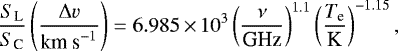 (1)
(1)
where SL and SC are the peak flux of RRL and flux of free–free continuum, respectively, and Te is the electron temperature. Adopting Te = 8000 K (see Mehringer et al. 1993), we derive the corresponding free–free continuum level of the four stacked RRLs (RRL-derived free–free emission, hereafter RFE). The comparison between the RFE and the continuum emission at the four frequencies is shown in Fig. 9. The observed continuum emission is supposed to be a mixture of free–free and synchrotron emission, which should have a higher intensity than the RFE maps. However, the RFE exceeds the observed continuum by a factor of ~ 2 at the low frequency end. One possible origin of this excess is that the RRLs are not under LTE conditions but stimulated.
To characterize the stimulation of RRLs, we introduce the RRL peak ratio η. According to theoretical models, the peak intensity of stimulated RRLs and frequency are anti-correlated at high frequencies (Shaver 1978). Therefore, we consider the RRLs at 8.9 and 10.5 GHz and define
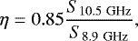 (2)
(2)
where S10.5 GHz and S8.9 GHz are the RRL peak intensities, respectively, while the normalization factor 0.85= 8.9∕10.5 result in η = 1 when LTE conditions hold. When the RRLs are stimulated, η < 1. In Fig. 10 we show the η map of DS.From the plot, we see that in the central and western part of DS, η ≈ 1, which indicates that the emission is under LTE. At the eastern edge of DS, we find η < 1, which suggests the presence of stimulated emission. Notably, source AA displays η = 1, meaning that its emission is under LTE, which is consistent with the scenario that source AA is an H II region with only thermal emission.
We quantify the correlation between non-thermal emission and the stimulation of RRLs, by plotting η against α pixel by pixel (see Fig. 11). A total of 63% of the pixels in DS have α < −0.1, meaning associated with non-thermal emission. Among these non-thermal pixels, 86% (53% of all the pixels in DS) have η < 1, i.e., the RRLs are stimulated under non-LTE conditions. Out of all the pixels, 58% have η < 1. The vast majority (92%) are associated with non-thermal emission. Therefore, most of the area in DS associated with non-thermal emission is also associated with stimulated RRLs, and similarly, almost all the parts associated with stimulated RRLs show non-thermal emission. The correlation between α and η seen in Fig. 11 is consistent with the scenario that RRLs can be stimulated by non-thermal emission (Shaver 1978).
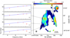 |
Fig. 8 Right: spectral index map of the Sgr B2(DS) as shown in the central panel of Fig. 5. The map of the uncertainty of spectral index is as shown in the right panel of Fig. 4. Left: peak intensities of the four stacked RRLs (see Table 1) at four selected positions. Position (a) corresponds to the well-known H II region AA, while the other positions have been selected to probe regions with negative spectral indices. The dashed line in each panels marks the scenario for LTE under which the flux is proportional to the frequency. |
5 Origin of thermal and non-thermal emission
We have found that the DS region, located within the envelope of Sgr B2, shows a mix of thermal free–free and non-thermal synchrotron continuum emission at radio wavelengths. This kind of radio continuum emission may have different origins: H II regions, supernova remnants (SNRs), planetary nebulae (PNe) or extragalactic radio sources. Although the most probable origin is the H II region, we have explored the other three scenarios. We searched the XMM-Newton catalog for X-ray sources in the region, and found no source associated with DS in the 0.5–12 keV continuum bands (Ponti et al. 2015). The lack of bright X-ray emission suggests that we can exclude a scenario in which DS is a SNR. In a different scenario, PNe can emit in the radio regime, however, their typical size ranges from 0.03 to 0.1 pc, i.e., significantly smaller than the radius of DS (0.5 pc). Additionally, the age of PNe is expected to be between 107 and 1010 yr (e.g., Bressan et al. 1993), much longer than the age of Sgr B2 (estimated to be about 0.74 Myr, see Kruijssen et al. 2015). Also, we estimate the total mass of the ionized gas in DS to be ~ 500 M⊙, which is much larger than the mass of a typical low-mass star that can generate a PN. Therefore, we exclude the possibility that DS is a PN. The minimum detectable flux density of our images is ~ 0.2 mJy, which can be used to estimate the expectable number of extragalactic radio sources. In the entire area of Sgr B2 (7′ × 7′), the expectednumber of extragalactic radio sources is ~1, while in the 1′ × 1′ area of DS, the number is ~0.03 (see Condon et al. 1998; Anglada et al. 1998). Additionally, the spatial extension of DS (~ 1′) is significantly larger than the typical size of extragalactic radio sources (see Condon et al. 1998). Therefore, the possibility that DS is an extragalactic radio source is excluded. Thus, the only remaining scenario is DS being an H II region. In this section, we discuss the properties of the central star and the possible mechanisms that can produce the observed non-thermal emission.
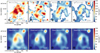 |
Fig. 9 Top panels: free–free continuum maps of the Sgr B2(DS) region derived from the four staked RRLs (RFE as described in Sect. 4.2, following Eq. (1)) at 4.4, 6.8, 8.9, and 10.5 GHz. Bottom panel: observed continuum emission at 4.4, 6.8, 8.9 and 10.5 GHz. For comparison, the observed continuum maps are also smoothed to 8′′, the beam is shown as the shaded circle in the lower left of each plot. |
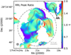 |
Fig. 10 Map of η (see Sect. 4.2) in DS. The X band continuum emission is overlaid as contours. The synthesized beam, corresponding to 8′′, is plotted as a dark circle at the lower left corner. The dashed circle indicates the area in which pixels are taken into account for Fig. 11. |
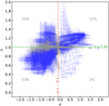 |
Fig. 11 η against spectral index (α). Only the pixels that are in the area marked by the dashed circle in Fig. 10 are taken into account, thus the influence of source AA is excluded. The criterion of non-thermal emission, α = −0.1, is shown with a vertical dashed line, while the criterion of stimulated RRL emission, η = 1, is shown as a horizontal dashed line. These two orthogonal lines divide the whole α–η space into four quadrants. For each quadrant, the number of pixels within it as a percentage of the number of all the pixels is written. The points with error bars crossing the α = −0.1 or η = 1 lines are colored gray and neglected in the statistics. |
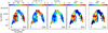 |
Fig. 12 Maps of shock velocity (U), volume density (n), and magnetic field strength (B) of DS that reproduce the observed flux density maps at the 12 frequencies (see Fig. 3) by the First-order Fermi acceleration model through a χ2 test using the model described in Padovani et al. (2019). The model also generates the modeled spectral index (αmod) map which isconsistent with the observed αobs map. |
5.1 Ionization by a central star
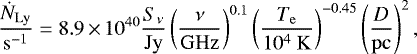
The flux of Lyman continuum photons, ṄLy, needed to ionized an H II region can be derived as following (Schmiedeke et al. 2016):
 (3)
(3)
where Sν is the flux at frequency ν, Te is the electron temperature, and D is the distance to the source. The total flux of the free–free emission in DS is 0.5 Jy at 11.2 GHz, assuming that the continuum emission at this frequency is pure thermal. For a typical H II region, the electron temperature ranges from 5000 to 10 000 K (Zuckerman et al. 1967). Taking D = 8.34 kpc for Sgr B2, we obtain a flux of Lyman continuum photons of 4–6 × 1048 s−1. Such a Lyman continuum flux corresponds to an O 7 ZAMS star (see Table II of Panagia 1973). We have searched the Spitzer infrared images (e.g., Ramírez et al. 2008) for a possible infrared counterpart of the star ionizing the H II region in DS, but found no clear candidate. Also the young stellar object catalog of Yusef-Zadeh et al. (2009) does not show any infrared source in the center of DS. One possible reason for the lack of a detected infrared source in DS is the high extinction. Assuming a column density of molecular hydrogen of 1024 cm−2 in DS (Schmiedeke et al. 2016; Ginsburg et al. 2018), the extinction at 5 μm is ~ 20, based on the grainmodel by Li & Draine (2001). For an O 7 star at a distance of 8.34 kpc, this extinction result in an apparent magnitude ~ 30, which is non-detectable in current infrared images.
5.2 Non-thermal emission origin
The interaction between cosmic-ray nuclei and the interstellar medium produces secondary electrons (and positrons). These secondary electrons can be a source of synchrotron emission like the one detected in Sgr B2(DS). Protheroe et al. (2008) analyze diffusion models and indicate that for secondary electrons to radiate synchrotron emission at GHz frequencies in ~ 1 mG magnetic field, cosmic-ray particles should have multi-GeV energies, whereas such cosmic-ray particles cannot penetrate into the cloud due tothe high gas density in Sgr B2 (see, e.g., Padovani et al. 2009, 2013). Thus, the penetration of cosmic rays from outside (e.g., from the nearby Galactic center) is excluded as a possible origin to the non-thermal emission observed in Sgr B2(DS).
However, the presence of synchrotron emission is the fingerprint of relativistic electrons. Padovani et al. (2015, 2016) showed thatparticle acceleration can take place at a shock location in protostars according to the first-order Fermi acceleration mechanism (also known as diffusive shock acceleration). In fact, local thermal particles are accelerated up to relativistic energies while crossing back and forth a shock surface thanks to magnetic fluctuations around the shock itself.
In a companion paper (Padovani et al. 2019), we present an extension to this theory applied to H II regions. We demonstrate that electrons can be efficiently accelerated under the hypothesis that the flow velocity in the reference frame of an expanding H II region hitting denser material is sufficiently high (> 35 km s−1) to switch onparticle acceleration. The main parameters of the model are the magnetic field strength, the flow velocity in the shock reference frame (hereafter velocity), the temperature, the volume density, and the ionization fraction. Assuming a complete ionized medium and a temperature of 8000 K (see Sect. 4.2), we studied the parameter space volume density-magnetic field strength and computed the emerging shock-accelerated electron flux for a shock radius of 0.36 pc, which is the average distance between the center of DS and the inner surface of the synchrotron emitting region. This electron flux is used to compute the synchrotron emissivity and then the flux density between 4 and 12 GHz for a beam of 4′′ and an average emitting region size3 of 0.85 pc. We performed a χ2 test to find the values of the velocity (U), density (n), and magnetic field strength (B) that best reproduce the observations. For the flux densities we obtain an average accuracy of about 20% assuming 33 ≲ U ≲ 50 km s−1, 104 ≲ n∕cm−3 ≲ 9 × 10⁴, and 0.3 ≲ B∕mG ≲ 4. From the model, we derive maps of the velocity, magnetic field strength and density in the Sgr B2(DS) region (see Fig. 12). The magnetic field strength is found to be in the range 0.5–2 mG as reported by Crutcher et al. (1996). The model also gives an α map of DS, which is in agreement with the observed α map (Fig. 5). It is interesting to notice that the velocity is lower where the density is higher. One reason might be that the flow is moving faster towards the east-west direction, which is the direction of minimum resistance. In contrast, the velocity is lower toward the northern direction where the density is higher. Although the RRL line width cannot be directly used to determine the shock speed, we note that it is significantly larger than the typical expansion velocity of an H II region (10 km s−1 Draine 2011), which points to an additional mechanism of acceleration. One possible origin of the high velocity is the presence of a stellar wind driven by the O 7 star that likely ionizes the H II region (see e.g., Veena et al. 2016; Pereira et al. 2016; Kiminki et al. 2017). We note that velocities of about 35 km s−1 are in agreement with what is obtained by simulations of H II regions of O and B stars driving strong stellar winds (Steggles et al. 2017).
It is important to remark that the flux densities (from which the spectral index is derived) estimated by our model are based on the assumption that all the parameters (magnetic field strength, velocity, temperature, density, and ionization fraction) are constant along the line of sight. For a proper modeling, one should account for the spatial variations of these quantities. However, the fact that model results are already fairly comparable with observations is an indication that shock-accelerated electrons may represent the key to explain the synchrotron emission in Sgr B2(DS). Previous studies (e.g., Yusef-Zadeh et al. 2007a,b, 2013, 2016) indicate that cosmic-ray induced non-thermal emission is common in the Galactic center region. On large scales, where the density is not as high as in the envelope of SgrB2, cosmic rays may play a dominant role in the production of relativistic electrons, while in extremely dense regions (and smaller scales, like Sgr B2(DS)) H II region shocks may be a dominant source of non-thermal emission.
6 Summary
We have observed the giant molecular cloud Sgr B2 with the VLA in its D and CnB configurations. We obtained continuum and RRL maps in the frequency range 4–12 GHz, covering a spatial extent of about 20′ × 20′, with a beam size of 4′′. We have focused our study on the Sgr B2(DS) region, located in the southern area of the Sgr B2 envelope. Our main results are:
-
Sgr B2(DS) is bright at radio wavelengths, with intensities in the range 10–50 mJy beam−1, within the observed 4 to 12 GHz frequency range. At 4′′ resolution, DS appears as bubble-like H II region with a diameter of about 1.5 pc, powered by an O 7 star, and surrounded by dense gas and a series of dense cores distributed in an arc structure around it.
-
We find that the total flux of DS decreases from 1.9 Jy at 4 GHz down to 0.5 Jy at 12 GHz. Spectral analysis shows that the spectral index of DS varies from − 0.4 to − 1.2, suggesting the presence of non-thermal emission, in addition to the thermal emission of the H II region. We decompose the thermal and non-thermal components in DS, and find that the thermal emission is clumpy and concentrated in the eastern lobe of the bubble-like structure, while the non-thermal emission appears widespread over the whole region.
-
The emission of RRLs in DS show a central velocity varying from 70 km s−1 in the center to 55 km s−1 in the outer edge. The line widths of the RRLs range from 30 to 40 km s−1. From the RRLs integrated intensity, we derive the corresponding thermal continuum emission, which exceeds the observedcontinuum by a factor of about 2 at the low frequency end. In addition, the RRLs intensity does not follow the Sν ∝ ν relation expected for RRLs under LTE conditions, but drops at high frequencies likely due to non-LTE effects. We find a correlation between the presence of non-thermal emission (i.e., negative spectral indices) and those regions where RRLs are excited under non-LTE conditions. This suggests that RRLs in Sgr B2(DS) are possibly stimulated by synchrotron emission.
-
We modeled the observed synchrotron emission, and found that relativistic electrons can be produced via first-order Fermi acceleration, which is triggered by the interaction between the expanding H II region and the denser surrounding material. The model, which is presented in a companion paper of Padovani et al. (2019), reproduces the observed flux density and spectral index. From the model, we derive maps of the flow velocity in the shock reference frame, magnetic field strength and density in the Sgr B2(DS) region. Velocities are found to be between 35 and 50 km s−1 as found in simulations of cometary H II regions of O and B stars driving strong stellar winds. The magnetic field strength is found to be in the range 0.3–4 mG as reported by Crutcher et al. (1996) and the density in the range of 1 − 9 × 104 cm−3.
In this work we have characterized the non-thermal emission observed towards the H II region Sgr B2(DS), and we have proposed that locally accelerated particles, under certain conditions of density, magnetic field, and shock velocity, can be the origin of the non-thermal emission. This result raises the question whether other H II regions may also show non-thermal emission. A handful of H II regions have been reported to have negative spectral indices suggestive of a non-thermal component (e.g., Garay et al. 1996; Veena et al. 2016, 2019), indicating that the presence of non-thermal emission in H II regions may be a more common event than previously thought. The advent of extremely sensitive facilities at radio wavelengths such as SKA (Square Kilometer Array) or the ngVLA (next generation Very Large Array) may trigger the systematic search for H II regions with non-thermal emission, thus allowing a study of the conditions under which non-thermal emission exists.
Acknowledgements
We thank the referee for his/her comments during the reviewing process.. F.M., A.S.M., P.S., A.S. research is carried out within the Collaborative Research Centre 956, sub-projects A6 and C3, funded by the Deutsche Forschungsgemeinschaft (DFG) - project ID 184018867. MP acknowledges funding from the European Unions Horizon 2020 research and innovation program under the Marie Skłodowska-Curie grant agreement No 664931. This research made use of Astropy4, a community-developed core Python package for Astronomy (Astropy Collaboration 2013, 2018).
Appendix A Intensityprofiles
In Fig. A.1 we plot the intensity profiles of the twelve channel maps across the Sgr B2(DS) region. The profiles are taken along the RA direction from (17:47:05, −28:25:10) to (17:47:38, −28:25:10). Since we set uv limit to 0.6–50 kλ, the large scale structures are filtered out, resulting in the background intensity to be ~ 0.
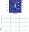 |
Fig. A.1 Top panel: continuum emission image of Sgr B2 at 4 GHz. The dashed line indicates the trajectory along which we get the intensity profile. Bottom panels: intensity profiles of the twelve channel maps. The uv limit of the twelve images has been set to 0.6–50 kλ and the images have been convolved to a circular beam of 4′′. The dashed line indicates the zero intensity level. |
Appendix B Combining GMRT and VLA
In this section we make use of recently observed GMRT observations to confirm the negative spectral indices measured towards the Sgr B2(DS) region. The GMRT observations were taken under the project number (31_021) and will be presented in detail in a forthcoming publication. In summary, we used the GMRT to observe the Galactic center at 350 MHz, with a total bandwidth of 32 MHz. The observations were centered at the position of Sgr B2. For comparison with the VLA data, we have selected data in the uv range 0.6–25 kλ. The short spacing is set to 0.6 kλ to match the same scales recovered in the VLA data. The synthesized beam of the GMRT image is 12.′′2 × 11.′′7 (PA= 57°). We have convolved the VLA images to the same resolution of the GMRT data, which results in the upper limit of the uv range for both the GMRT and VLA images to be ~ 25 kλ.
We obtain the spectral index in DS by interpolating the flux density between the 350 MHz and 12 GHz images. As shown in the right panel of Fig. B.1, the spectral index in DS is negative and in agreement with the spectral index values determined using the VLA data (cf. Fig. 4). In the left panels of Fig. B.1 we show the SED of the 13 channel images for two positions in DS. The SEDs in these positions can be describe by a combination of thermal and non-thermalemission, in agreement with the analysis based on the VLA data. However, the relatively coarse angular resolution of the GMRT images makes the study of the small-scale structure of the DS bubble not possible. Therefore, in this paper, we focus on the analysis of the VLA images and the sub-pc structures in DS. A complete analysis of the GMRT data will be used to study the large-scale structure of the Galactic center region in a forthcoming paper (Meng et al., in prep.).
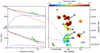 |
Fig. B.1 Right panel: spectral index image obtained from the 350 MHz GMRT emission map (Meng et al., in prep.) and the 4 GHz VLA continuum image. Both images have been obtained after limiting the short uv to 0.6 kλ, and convolving the images to a common beam of 12.2′′ × 11.7′′ (PA = 57°), which corresponds to ~25 kλ. Left panel: two examples of SEDs for two selected positions within DS. The observed fluxes are shown with green symbols, all of them measured from images with same spatial filtering and synthesized beam. For illustration, the thermal (blue dashed curve), non-thermal (red dashed line) and the mixed (black solid curve) components are marked. The curves are just qualitative descriptions of the possible contribution of the thermal and non-thermal components, and do not aim at fitting the data. |
Appendix C The RRL maps
In this section we show the maps of fit parameters of the four stacked RRLs (see Table 1). The fit parameters include integrated intensity, centroid velocity, line width, and peak intensity (see Fig. C.1).
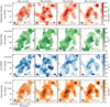 |
Fig. C.1 Maps of the fit parameters of RRLs in DS. From top to bottom the four rows: the integrated intensity, centroid velocity, line width, and peak intensity. The RRLs are fit with a Gaussian function. The synthesized beam (8 arcsec) is shown at the lower left corner of each panel. Continuum emission at respective frequencies (4.4, 6.8, 8.9 and 10.5 GHz) are overlaid as contours. |
References
- Anglada, G., Villuendas, E., Estalella, R., et al. 1998, AJ, 116, 2953 [NASA ADS] [CrossRef] [Google Scholar]
- Astropy Collaboration (Robitaille, T. P., et al.) 2013, A&A, 558, A33 [NASA ADS] [CrossRef] [EDP Sciences] [Google Scholar]
- Astropy Collaboration (Price-Whelan, A. M., et al.) 2018, AJ, 156, 123 [Google Scholar]
- Bressan, A., Fagotto, F., Bertelli, G., & Chiosi, C. 1993, A&AS, 100, 647 [NASA ADS] [Google Scholar]
- Condon, J. J., Cotton, W. D., Greisen, E. W., et al. 1998, AJ, 115, 1693 [NASA ADS] [CrossRef] [Google Scholar]
- Crutcher, R. M., Roberts, D. A., Mehringer, D. M., & Troland, T. H. 1996, ApJ, 462, L79 [NASA ADS] [CrossRef] [Google Scholar]
- De Pree, C. G., Goss, W. M., & Gaume, R. A. 1998, ApJ, 500, 847 [NASA ADS] [CrossRef] [Google Scholar]
- De Pree, C. G., Peters, T., Mac Low, M.-M., et al. 2014, ApJ, 781, L36 [NASA ADS] [CrossRef] [Google Scholar]
- Draine, B. T. 2011, Physics of the Interstellar and Intergalactic Medium (New Jersey: Princeton University Press) [Google Scholar]
- Garay, G., Ramirez, S., Rodriguez, L. F., Curiel, S., & Torrelles, J. M. 1996, ApJ, 459, 193 [NASA ADS] [CrossRef] [Google Scholar]
- Gaume, R. A., Claussen, M. J., de Pree, C. G., Goss, W. M., & Mehringer, D. M. 1995, ApJ, 449, 663 [NASA ADS] [CrossRef] [Google Scholar]
- Ginsburg, A., Henkel, C., Ao, Y., et al. 2016, A&A, 586, A50 [NASA ADS] [CrossRef] [EDP Sciences] [Google Scholar]
- Ginsburg, A., Bally, J., Barnes, A., et al. 2018, ApJ, 853, 171 [NASA ADS] [CrossRef] [Google Scholar]
- Goldsmith, P. F., Lis, D. C., Hills, R., & Lasenby, J. 1990, ApJ, 350, 186 [NASA ADS] [CrossRef] [Google Scholar]
- Gravity Collaboration (Abuter, R., et al.) 2018, A&A, 615, L15 [NASA ADS] [CrossRef] [EDP Sciences] [Google Scholar]
- Hollis, J. M., Pedelty, J. A., Boboltz, D. A., et al. 2003, ApJ, 596, L235 [NASA ADS] [CrossRef] [Google Scholar]
- Hollis, J. M., Jewell, P. R., Remijan, A. J., & Lovas, F. J. 2007, ApJ, 660, L125 [NASA ADS] [CrossRef] [Google Scholar]
- Jones, D. I., Crocker, R. M., Ott, J., Protheroe, R. J., & Ekers, R. D. 2011, AJ, 141, 82 [NASA ADS] [CrossRef] [Google Scholar]
- Kiminki, M. M., Smith, N., Reiter, M., & Bally, J. 2017, MNRAS, 468, 2469 [NASA ADS] [CrossRef] [Google Scholar]
- Kruijssen, J. M. D., Dale, J. E., & Longmore, S. N. 2015, MNRAS, 447, 1059 [NASA ADS] [CrossRef] [Google Scholar]
- Kurtz, S. 2002, in Hot Star Workshop III: The Earliest Phases of Massive Star Birth, ed. P. Crowther, ASP Conf. Ser., 267, 81 [NASA ADS] [Google Scholar]
- Kurtz, S. 2005, IAU Symp., 227, 111 [NASA ADS] [CrossRef] [Google Scholar]
- LaRosa, T. N., Kassim, N. E., Lazio, T. J. W., & Hyman, S. D. 2000, AJ, 119, 207 [NASA ADS] [CrossRef] [Google Scholar]
- LaRosa, T. N., Brogan, C. L., Shore, S. N., et al. 2005, ApJ, 626, L23 [NASA ADS] [CrossRef] [Google Scholar]
- Law, C. J., Yusef-Zadeh, F., & Cotton, W. D. 2008, ApJS, 177, 515 [NASA ADS] [CrossRef] [Google Scholar]
- Li, A., & Draine, B. T. 2001, ApJ, 554, 778 [Google Scholar]
- Martín-Pintado, J., Gaume, R. A., Rodríguez-Fernández, N., de Vicente, P., & Wilson, T. L. 1999, ApJ, 519, 667 [NASA ADS] [CrossRef] [Google Scholar]
- McMullin, J. P., Waters, B., Schiebel, D., Young, W., & Golap, K. 2007, in Astronomical Data Analysis Software and Systems XVI, eds. R. A. Shaw, F. Hill, & D. J. Bell, ASP Conf. Ser., 376, 127 [NASA ADS] [Google Scholar]
- Mehringer, D. M., Palmer, P., Goss, W. M., & Yusef-Zadeh, F. 1993, ApJ, 412, 684 [NASA ADS] [CrossRef] [Google Scholar]
- Mücke, A., Koribalski, B. S., Moffat, A. F. J., Corcoran, M. F., & Stevens, I. R. 2002, ApJ, 571, 366 [NASA ADS] [CrossRef] [Google Scholar]
- Padovani, M., Galli, D., & Glassgold, A. E. 2009, A&A, 501, 619 [NASA ADS] [CrossRef] [EDP Sciences] [Google Scholar]
- Padovani, M., Hennebelle, P., & Galli, D. 2013, A&A, 560, A114 [NASA ADS] [CrossRef] [EDP Sciences] [Google Scholar]
- Padovani, M., Hennebelle, P., Marcowith, A., & Ferrière, K. 2015, A&A, 582, L13 [NASA ADS] [CrossRef] [EDP Sciences] [Google Scholar]
- Padovani, M., Marcowith, A., Hennebelle, P., & Ferrière, K. 2016, A&A, 590, A8 [NASA ADS] [CrossRef] [EDP Sciences] [Google Scholar]
- Padovani, M., Marcowith, A., Sánchez-Monge, Á., Meng, F., & Schilke, P. 2019, A&A, 630, A72 [NASA ADS] [CrossRef] [EDP Sciences] [Google Scholar]
- Panagia, N. 1973, AJ, 78, 929 [NASA ADS] [CrossRef] [Google Scholar]
- Pereira, V., López-Santiago, J., Miceli, M., Bonito, R., & de Castro, E. 2016, A&A, 588, A36 [NASA ADS] [CrossRef] [EDP Sciences] [Google Scholar]
- Perley, R. A., & Butler, B. J. 2013, ApJS, 204, 19 [NASA ADS] [CrossRef] [Google Scholar]
- Platania, P., Bensadoun, M., Bersanelli, M., et al. 1998, ApJ, 505, 473 [NASA ADS] [CrossRef] [Google Scholar]
- Pols, S., Schwörer, A., Schilke, P., et al. 2018, A&A, 614, A123 [NASA ADS] [CrossRef] [EDP Sciences] [Google Scholar]
- Ponti, G., Morris, M. R., Terrier, R., et al. 2015, MNRAS, 453, 172 [NASA ADS] [CrossRef] [Google Scholar]
- Protheroe, R. J., Ott, J., Ekers, R. D., Jones, D. I., & Crocker, R. M. 2008, MNRAS, 390, 683 [NASA ADS] [Google Scholar]
- Ramírez, S. V., Arendt, R. G., Sellgren, K., et al. 2008, ApJS, 175, 147 [NASA ADS] [CrossRef] [Google Scholar]
- Reid, M. J., Menten, K. M., Brunthaler, A., et al. 2014, ApJ, 783, 130 [Google Scholar]
- Sánchez-Monge, Á., Kurtz, S., Palau, A., et al. 2013, ApJ, 766, 114 [NASA ADS] [CrossRef] [Google Scholar]
- Sánchez-Monge, Á., Schilke, P., Schmiedeke, A., et al. 2017, A&A, 604, A6 [NASA ADS] [CrossRef] [EDP Sciences] [Google Scholar]
- Schmiedeke, A., Schilke, P., Möller, T., et al. 2016, A&A, 588, A143 [NASA ADS] [CrossRef] [EDP Sciences] [Google Scholar]
- Schwörer, A., Sánchez-Monge, Á., Schilke, P., et al. 2019, A&A, 628, A6 [NASA ADS] [CrossRef] [EDP Sciences] [Google Scholar]
- Shaver, P. A. 1978, A&A, 68, 97 [NASA ADS] [Google Scholar]
- Steggles, H. G., Hoare, M. G., & Pittard, J. M. 2017, MNRAS, 466, 4573 [NASA ADS] [CrossRef] [Google Scholar]
- Veena, V. S., Vig, S., Tej, A., et al. 2016, MNRAS, 456, 2425 [NASA ADS] [CrossRef] [Google Scholar]
- Veena, V. S., Vig, S., Sebastian, B., et al. 2019, MNRAS, 482, 4630 [NASA ADS] [CrossRef] [Google Scholar]
- Yusef-Zadeh, F., Muno, M., Wardle, M., & Lis, D. C. 2007a, ApJ, 656, 847 [NASA ADS] [CrossRef] [Google Scholar]
- Yusef-Zadeh, F., Wardle, M., & Roy, S. 2007b, ApJ, 665, L123 [NASA ADS] [CrossRef] [Google Scholar]
- Yusef-Zadeh, F., Hewitt, J. W., Arendt, R. G., et al. 2009, ApJ, 702, 178 [NASA ADS] [CrossRef] [Google Scholar]
- Yusef-Zadeh, F., Wardle, M., Lis, D., et al. 2013, J. Phys. Chem. A, 117, 9404 [CrossRef] [Google Scholar]
- Yusef-Zadeh, F., Cotton, W., Wardle, M., & Intema, H. 2016, ApJ, 819, L35 [NASA ADS] [CrossRef] [Google Scholar]
- Zuckerman, B., Palmer, P., Penfield, H., & Lilley, A. E. 1967, ApJ, 149, L61 [NASA ADS] [CrossRef] [Google Scholar]
A new distance to the Galactic center has been measured to be 8.127 ± 0.031 kpc (Gravity Collaboration 2018). For consistency with the paper published within the same series of studies of Sgr B2, we use the distance reported by Reid et al. (2014).
All Tables
All Figures
|
Fig. 1 Continuum images of Sgr B2 in C (panel a) and X (panel b) bands. Relevant regions are marked with their names (see Mehringer et al. 1993). The dashed boxes mark the region of DS. The synthesized beam of the C and X images are 2.7′′ × 2.5′′ and 1.82′′ × 1.53′′, respectively |
| In the text | |
|
Fig. 2 C band (4–8 GHz) continuum emission map of Sgr B2(DS). The circles mark the positions of the high-mass protostellar cores identified by Ginsburg et al. (2018). The synthesized beam is shown as a yellow ellipse at the bottom left corner. |
| In the text | |
|
Fig. 3 Channel maps of the Sgr B2(DS) region. All the 12 maps have been produced considering the same uv range limited to 0.6–50 kλ, and have been convolved to a circular beam of 4′′. The synthesized beam is shown as a yellow circle in the bottom left panel. |
| In the text | |
|
Fig. 4 Spectral index (α, panel a) andits uncertainty, (panel b) throughout the whole Sgr B2 region. The regions marked in both panels correspond to those regions also labeled in Fig. 1. See Sect. 3.2 for details in the calculation of the spectral index. |
| In the text | |
|
Fig. 5 Spectral index of DS. Six spots are taken as examples to show the fitting of SED and the fit spectral index (α). The contours are where the flux density at 4 GHz is 10 mJ beam−1. The angular resolution is 4′′ × 4′′, and the beam is shown in the lower left corner. |
| In the text | |
|
Fig. 6 Spatial distribution of synchrotron (or non-thermal, left panel), mixed (central panel, corresponding to observed image) and free–free (or thermal, right panel) components of DS at 4 GHz as derived from method described in Sect. 4.1.1. The thermal emission map is extrapolated from 12 GHz assuming that at this frequency the emission is originated by a thermal component with a spectral index α = −0.1. The non-thermal emission is obtained by subtracting the extrapolated thermal emission from the mixed emission. The contours are the same as in Fig. 5. All panels have a circular beam of 4′′ (shown in the bottom left corner of each panel). The dashed circles indicate the region in which we calculate the flux density of DS (see Sect. 4.1). |
| In the text | |
|
Fig. 7 Spatial distribution of the synchrotron (left panel), mixed (central panel) and free–free (right panel) components of DS at 4 GHz. All the three images are obtained after fitting the observed SED with the sum of two power-law functions: Sth (ν) ∝ ν−0.1 and Snt (ν) ∝ ν−0.7 for the thermal and non-thermal components, respectively (see details in Sect. 4.1.2). The contours are the same as in Fig. 5. All panels have a circular beam of 4′′ (shown in the bottom left corner of each panel). The dashed circles indicate the region in which we calculated the flux density of DS (see Sect. 4.1). |
| In the text | |
|
Fig. 8 Right: spectral index map of the Sgr B2(DS) as shown in the central panel of Fig. 5. The map of the uncertainty of spectral index is as shown in the right panel of Fig. 4. Left: peak intensities of the four stacked RRLs (see Table 1) at four selected positions. Position (a) corresponds to the well-known H II region AA, while the other positions have been selected to probe regions with negative spectral indices. The dashed line in each panels marks the scenario for LTE under which the flux is proportional to the frequency. |
| In the text | |
|
Fig. 9 Top panels: free–free continuum maps of the Sgr B2(DS) region derived from the four staked RRLs (RFE as described in Sect. 4.2, following Eq. (1)) at 4.4, 6.8, 8.9, and 10.5 GHz. Bottom panel: observed continuum emission at 4.4, 6.8, 8.9 and 10.5 GHz. For comparison, the observed continuum maps are also smoothed to 8′′, the beam is shown as the shaded circle in the lower left of each plot. |
| In the text | |
|
Fig. 10 Map of η (see Sect. 4.2) in DS. The X band continuum emission is overlaid as contours. The synthesized beam, corresponding to 8′′, is plotted as a dark circle at the lower left corner. The dashed circle indicates the area in which pixels are taken into account for Fig. 11. |
| In the text | |
|
Fig. 11 η against spectral index (α). Only the pixels that are in the area marked by the dashed circle in Fig. 10 are taken into account, thus the influence of source AA is excluded. The criterion of non-thermal emission, α = −0.1, is shown with a vertical dashed line, while the criterion of stimulated RRL emission, η = 1, is shown as a horizontal dashed line. These two orthogonal lines divide the whole α–η space into four quadrants. For each quadrant, the number of pixels within it as a percentage of the number of all the pixels is written. The points with error bars crossing the α = −0.1 or η = 1 lines are colored gray and neglected in the statistics. |
| In the text | |
|
Fig. 12 Maps of shock velocity (U), volume density (n), and magnetic field strength (B) of DS that reproduce the observed flux density maps at the 12 frequencies (see Fig. 3) by the First-order Fermi acceleration model through a χ2 test using the model described in Padovani et al. (2019). The model also generates the modeled spectral index (αmod) map which isconsistent with the observed αobs map. |
| In the text | |
|
Fig. A.1 Top panel: continuum emission image of Sgr B2 at 4 GHz. The dashed line indicates the trajectory along which we get the intensity profile. Bottom panels: intensity profiles of the twelve channel maps. The uv limit of the twelve images has been set to 0.6–50 kλ and the images have been convolved to a circular beam of 4′′. The dashed line indicates the zero intensity level. |
| In the text | |
|
Fig. B.1 Right panel: spectral index image obtained from the 350 MHz GMRT emission map (Meng et al., in prep.) and the 4 GHz VLA continuum image. Both images have been obtained after limiting the short uv to 0.6 kλ, and convolving the images to a common beam of 12.2′′ × 11.7′′ (PA = 57°), which corresponds to ~25 kλ. Left panel: two examples of SEDs for two selected positions within DS. The observed fluxes are shown with green symbols, all of them measured from images with same spatial filtering and synthesized beam. For illustration, the thermal (blue dashed curve), non-thermal (red dashed line) and the mixed (black solid curve) components are marked. The curves are just qualitative descriptions of the possible contribution of the thermal and non-thermal components, and do not aim at fitting the data. |
| In the text | |
|
Fig. C.1 Maps of the fit parameters of RRLs in DS. From top to bottom the four rows: the integrated intensity, centroid velocity, line width, and peak intensity. The RRLs are fit with a Gaussian function. The synthesized beam (8 arcsec) is shown at the lower left corner of each panel. Continuum emission at respective frequencies (4.4, 6.8, 8.9 and 10.5 GHz) are overlaid as contours. |
| In the text | |
Current usage metrics show cumulative count of Article Views (full-text article views including HTML views, PDF and ePub downloads, according to the available data) and Abstracts Views on Vision4Press platform.
Data correspond to usage on the plateform after 2015. The current usage metrics is available 48-96 hours after online publication and is updated daily on week days.
Initial download of the metrics may take a while.