| Issue |
A&A
Volume 628, August 2019
|
|
|---|---|---|
| Article Number | A19 | |
| Number of page(s) | 22 | |
| Section | Stellar structure and evolution | |
| DOI | https://doi.org/10.1051/0004-6361/201935453 | |
| Published online | 29 July 2019 | |
Mass transfer on a nuclear timescale in models of supergiant and ultra-luminous X-ray binaries
1
Argelander-Insitut für Astronomie, Universität Bonn, Auf dem Hügel 71, 53121 Bonn, Germany
e-mail: mquast@astro.uni-bonn.de
2
Max-Planck-Institut für Radioastronomie, Auf dem Hügel 69, 53121 Bonn, Germany
3
Aarhus Institute of Advanced Studies (AIAS), Aarhus University, Høegh-Guldbergs Gade 6B, 8000 Aarhus C, Denmark
4
Department of Physics and Astronomy, Aarhus University, Ny Munkegade 120, 8000 Aarhus C, Denmark
Received:
12
March
2019
Accepted:
12
May
2019
Context. The origin and number of the Galactic supergiant X-ray binaries is currently not well understood. They consist of an evolved massive star and a neutron star or black-hole companion. X-rays are thought to be generated from the accretion of wind material donated by the supergiant, while mass transfer due to Roche-lobe overflow is mostly disregarded because the high mass ratios of these systems are thought to render this process unstable.
Aims. We investigate how the proximity of supergiant donor stars to the Eddington limit, and their advanced evolutionary stage, may influence the evolution of massive and ultra-luminous X-ray binaries with supergiant donor stars (SGXBs and ULXs).
Methods. We constructed models of massive stars with different internal hydrogen and helium gradients (H/He gradients) and different hydrogen-rich envelope masses, and exposed them to slow mass-loss to probe the response of the stellar radius. In addition, we computed the corresponding Roche-lobe overflow mass-transfer evolution with our detailed binary stellar evolution code, approximating the compact objects as point masses.
Results. We find that a H/He gradient in the layers beneath the surface, as it is likely present in the well-studied donor stars of observed SGBXs, can enable mass transfer in SGXBs on a nuclear timescale with a black-hole or a neutron star accretor, even for mass ratios in excess of 20. In our binary evolution models, the donor stars rapidly decrease their thermal equilibrium radius and can therefore cope with the inevitably strong orbital contraction imposed by the high mass ratio. We find that the orbital period derivatives of our models agree well with empirical values. We argue that the SGXB phase may be preceded by a common-envelope evolution. The envelope inflation near the Eddington limit means that this mechanism more likely occurs at high metallicity.
Conclusion. Our results open a new perspective for understanding that SGBXs are numerous in our Galaxy and are almost completely absent in the Small Magellanic Cloud. Our results may also offer a way to find more ULX systems, to detect mass transfer on nuclear timescales in ULX systems even with neutron star accretors, and shed new light on the origin of the strong B-field in these neutron stars.
Key words: binaries: general / stars: massive / X-rays: binaries
© ESO 2019
1. Introduction
X-ray binaries represent an evolved stage of the evolution of massive binary systems (Verbunt et al. 1992; Tauris & van den Heuvel 2006; Marchant et al. 2017). They contain an ordinary star, the mass donor, and a compact object, namely a neutron star (NS) or a black hole (BH). In these systems, X-ray radiation is released by the accretion of matter that is released by the mass donor onto the compact companion (Frank et al. 2002). Depending on the mass of the donor star, X-ray binaries are divided into low-mass (LMXBs) and high-mass X-ray binaries (HMXBs).
High-mass X-ray binaries may also help us to understand rare ultra-luminous X-ray sources (ULXs; Kaaret et al. 2017), their more luminous cousins in the X-ray sky. Furthermore, HMXBs may be progenitors of merging BHs (Marchant et al. 2016) and NSs (Tauris et al. 2017), and thus have a direct connection to the gravitational-wave signals detected by the Virgo interferometer, which is part of the Laser Interferometer Gravitational-Wave Observatory (LIGO; Abbott et al. 2016, 2017). A study of HMXBs, their formation and evolution thus provides a better understanding of future results from gravitational-wave surveys.
While the mass-transfer and accretion processes in LMXBs are quite well understood (Tauris & van den Heuvel 2006), our knowledge of these processes in HMXBs is more limited. The mass-transfer mode in HMXBs is thought to be either wind accretion (Shakura et al. 2014) or Roche-lobe overflow (RLO; Savonije 1978). Because the first mode requires an extreme stellar wind with mass-loss rates of the order of several 10−5 M⊙ yr−1 to achieve the observed X-ray luminosities, this is only expected to occur in HMXBs. RLO is often thought to occur in LMXBs because it provides a sufficiently high mass-transfer rate to explain the luminous X-ray emission. In HMXBs, however, RLO is expected to lead to a rapid shrinking of the orbit as the result of the high mass ratio between the donor star and the accretor, leading to a common-envelope (CE) phase. Van den Heuvel et al. (2017) argued that systems with a mass ratio ≳3.5 would always undergo unstable RLO mass-transfer. This would mean that a system containing an O star (≳20 M⊙) and an NS (< 3 M⊙) would quickly enter a CE phase. In this case, the resulting X-ray lifetime cannot exceed the thermal timescale of the donor star. Savonije (1978) indeed found an X-ray lifetime of only 3 × 10⁴ yr for a system with a mass ratio of 16, which is of the order of the thermal timescale of the O star.
High-mass X-ray binaries are subdivided into two main groups (Lewin et al. 1995). The first group harbours an evolved O- or B-type supergiant. These systems typically have a short orbital period (Walter et al. 2015), indicating that the supergiant might be close to filling its Roche lobe. The two mass-transfer modes, wind mass-transfer and RLO, could explain the persistent and luminous X-ray emission. The binaries of the second, more numerous, subgroup consist of an early Be-type donor and a compact object. The appearance of emission lines indicates the existence of a circumstellar disc of material that is thought to be streaming off the nearly critically rotating B star along its equatorial plane. Orbiting its host, the compact object eventually penetrates this disc and accretes matter at this stage (Apparao 1985). This process is seen as a transient X-ray source recurring within a few 10–100 days, corresponding to the period of the wide and eccentric orbit. This inefficient accretion mode does not greatly affect the orbital separation. Thus, the expected X-ray lifetime is the main-sequence time of a B star, about a dozen million years. Building on this, Meurs & van den Heuvel (1989) estimated the total number of X-ray binaries in our galaxy that host supergiants (SGXB) and Be stars (BeXBs). Taking observational biases into account, they expected that about 30 SGXB and 3000 BeXBs host X-ray binaries in the Milky Way. The fraction of SGXBs to BeXBs reflects the ratio between their expected X-ray life times, that is, thermal to nuclear timescale, which is roughly 1/100. This estimate agreed well with observations at the time (Lewin et al. 1995).
Bird et al. (2007; see also Bird et al. 2010) discovered that some SGXBs show peculiar behaviour. While some of them show X-ray transients on a timescale of a few hours (Heise & in’t Zand 2006), a second group has a characteristic high absorption corresponding to a column density of NH ≥ 1023 cm−2 (Manousakis et al. 2012). The first subgroup of SGXBs is referred to as supergiant fast X-ray transients (SFXTs). The other group is called obscured SGXBs. The mechanisms leading to their formation as well as the role these mechanism play in the evolution of SGXBs are poorly understood. The configuration of the obscured SGXBs has been considered to extend from the existence of a cocoon of dust that enshrouds the whole system (Chaty et al. 2008) to an unusually slow and dense stellar wind (v∞ ∼ 400 km s−1) (Manousakis & Walter 2012). While a dust cocoon could indeed form as the result of CE evolution, it is not obvious why a supergiant donor should exhibit a very slow wind velocity because neither observations nor numerical calculations suggest such slow winds for single stars. It is therefore reasonable to assume that the high attenuation might be connected to the existence of a companion and is not an intrinsic attribute of a supergiant.
Recently, Walter et al. (2015) reported 20 new SGXBs and 8 new BeXBs found by ESA’s International Gamma-Ray Astrophyiscs Laboratory (INTEGRAL). This leads to a total number of 36 SGXBs and 60 BeXBs known in the Milky Way. The current observed number of supergiant systems therefore appears to be too high to be explained by thermal timescale RLO of SGXBs. A way to address this problem is to postulate wind accretion in SGXBs (Shakura et al. 2014; Bozzo et al. 2016). However, population synthesis studies by Dalton & Sarazin (1995) predicted a number ratio of SGXBs/BeXBs of ≲0.15, even if wind accretion is assumed to be the main mass-transfer mode.
On the other hand, stabilising processes during RLO are a highly debated field of research (Ivanova 2015; Dermine et al. 2009; Blondin & Owen 1997; Savonije 1979). Pratt & Strittmatter (1976) discussed mass-transfer stabilisation due to the rotational slow-down of the donor star, caused by tidal breaking, and the subsequently diminishing centrifugal force in its outer layers. Stabilisation by widening of the Roche-lobe due to mass loss by a stellar wind was studied by Basko et al. (1977). Hjellming & Webbink (1987) investigated mass transfer on dynamical timescales using semi-analytical models. They found that any initial stability due to the rapid adiabatic expansion of the primary’s outer layer will switch to an unstable mode if these layers are super-adiabatic. Tauris et al. (2000) discovered the possibility of long-term stable mass transfer even if the mass ratio exceeds a value of 4. More recently, Pavlovskii et al. (2017) showed that RLO can be stable if the primary is a post-main-sequence star (case B mass transfer) that has already expanded through the Hertzsprung gap but has not yet developed a deep convective envelope (see also Pavlovskii & Ivanova 2015).
A similar timescale problem as in the SGXBs may exist in some ULX sources, many of which radiate highly above the Eddington accretion limit of a ∼10 M⊙ BH (Long et al. 1981; Kaaret et al. 2017). An interesting case is the ULX NGC 7793 P13. In this source, X-ray pulses were discovered by Israel et al. (2017b), indicating that the companion is an NS. With an estimated donor star mass of ∼20 M⊙, the mass ratio of the system is high, such that, again, stable mass transfer is not expected to occur. However, wind accretion alone cannot explain the high X-ray luminosity. How NGC 7793 P13 and three more X-ray pulsating ULXs (Bachetti et al. 2014; Israel et al. 2017a; Maitra et al. 2018) form and transfer mass is therefore not well understood.
In this study, we work out conditions under which stable mass transfer on a nuclear timescale can occur even though the donor star is much more massive than the compact companion. We explain our methods for modelling single-star and binary evolution in Sect. 2, including mass transfer to a compact object, and work out the criteria for long-term RLO and the connection of these evolutions to the internal structure of the donor. In Sect. 3 we investigate the sensitivity of the donor star radius to mass loss, and we present our binary evolution models in Sect. 4, including examples of systems with high mass ratios that undergo mass transfer on a nuclear timescale. In Sect. 5 we discuss the possible properties of NS and BH hosting ULXs in the light of our findings. In Sect. 6 we investigate possible paths for the evolution of SGXB and ULX progenitors, and in Sect. 7 we discuss their likely evolutions. Our conclusions are presented in Sect. 8.
2. Method
2.1. Modelling stellar evolution and mass transfer
We used the binary evolution code (BEC), a one-dimensional hydrodynamic Lagrangian code, to solve the equations of stellar structure (Kippenhahn & Weigert 1990) and model the binary interaction (Braun & Langer 1993). The code includes up-to-date physics (Wellstein & Langer 1999; Wellstein et al. 2001) and uses the OPAL opacity tables (Iglesias & Rogers 1996). For convection zones, the mixing length theory (MLT) by Böhm-Vitense (1958) was applied, where we adopted αML = 1.0 unless stated otherwise. We note that the value of αML is uncertain (Pinheiro & Fernandes 2013) and may differ for stars in different evolutionary stages and/or mass ranges. Nevertheless, a mixing length parameter of the order of unity is in agreement with observations (Cox & Giuli 1968; Ferraro et al. 2006). The rotation and magnetic fields were not taken into account. For stellar wind mass loss, we followed the assumptions made by Brott et al. (2011), unless stated otherwise.
We investigated the case of X-ray binaries. We evolved an ordinary star with a point-mass companion that represents the NS or BH. The point mass induces mass transfer when the donor star exceeds its Roche radius, and mass is carried to the compact companion accretor via the first Lagrangian point. Here, the Roche lobe is approximated by a sphere of radius RL that has the same volume as the Roche lobe, following Eggleton (1983),
where q = MD/MA is the mass ratio of donor and accretor, and a is the orbital separation. The mass-transfer rate was calculated using the method of Kolb & Ritter (1990). When the donor star did not fill its Roche volume, we computed the accretion of stellar wind material onto the compact star using the description of Bondi & Hoyle (1944).
When matter falls onto the compact object, it heats up and releases a large portion of the gained gravitational energy in X-rays. This leads to a feedback on the remaining material, of which the radiative force may expel a certain fraction. Hence the accretion rate and therefore the X-ray luminosity are self-regulated and are usually not expected to exceed the Eddington-accretion rate and luminosity of this object (but see Sect. 4.6). When we write the Eddington luminosity of an accretor with mass MA as
the Eddington accretion rate can be expressed as
where η is the fraction of rest-mass energy of the accreted material that is released as radiation, and κ is the opacity. We adopted η = 0.06, assuming a non-rotating BH, and  for an NS. Furthermore, we assumed only electron-scattering opacity (Kippenhahn & Weigert 1990). Under these assumptions, we may calculate the Eddington-accretion rate as
where we distinguish between NSs and the more massive BHs. In this equation, X is the hydrogen mass fraction of the accreted material. The different scaling of the Eddington rate with respect to the accretor mass arises from different mass–radius relations of BHs and NSs. While the BHs Schwarzschild radius is proportional to its mass, the NSs radius scales as  for a perfect Fermi gas. The NS mass–radius relation was scaled such that a 2 M⊙ NS has a radius of 12 km (Demorest et al. 2010). We computed the actual accretion rate as the minimum of the mass-transfer rate ṀRLO and the Eddington rate given by Eq. (4), that is, ṀA = min [ṀRLO, ṀEdd].
2.2. Internal H/He gradients
Schootemeijer & Langer (2018) derived the internal hydrogen and Helium gradients (H/He gradients) in the hydrogen-rich Wolf–Rayet stars of the SMC. They found that these gradients are different by more than a factor of ten for different objects. Because we show below that these gradients can play a key role in stabilising the mass transfer in SGXBs, we consider it as a free parameter in our models.
We evolved three stellar models of solar metallicity (Brott 2011) and initial masses of 50 M⊙, 60 M⊙, and 80 M⊙ to core helium mass fractions of 0.6, 0.7, and 0.8.
Subsequently, we adjusted the helium profile by setting the helium mass fraction above the convective core to
![$$ \begin{aligned} Y(m)=\max \left[Y_\text{ core}+\frac{\mathrm{d} Y}{\mathrm{d} m}(m-m_\text{ core}),~0.2638 \right] , \end{aligned} $$](/articles/aa/full_html/2019/08/aa35453-19/aa35453-19-eq7.gif)
with prescribed fixed values of dY/dm. Here m and Y denote the Lagrangian mass coordinate and the helium abundance, mcore is the mass of the convective core, and Ycore is its helium abundance. We then relaxed the models thermally, disregarding changes in their chemical profile due to mixing or burning. Then we exposed the models to a constant mass-loss rate of 10−5 M⊙ yr−1, which is of the order of magnitude of the mass-transfer rate on a nuclear timescale, MD/τnuc, D, to the response of the stellar radius and derived the mass–radius exponent
The results of this exercise are presented in Sect. 3.1.
While the initial masses of our models are in general higher than the donor masses observed in SGXBs, the masses of the stellar models are in good agreement with observations after the artificial mass loss. The advantage of first producing very massive models and a consequent mass reduction is shown in Sect. 6, where this procedure will provide an interpretation of the over-luminosity found in SGXBs.
2.3. Response of the Roche radius
If mass is transferred from the donor to the accretor, the Roche radius RL changes due to changing orbital separation. We considered the orbital evolution by changes in stellar masses and hence in mass ratio, by angular momentum loss through the donor’s stellar wind, and by angular momentum loss by isotropic re-emission of matter near the compact object. Additional effects, such as spin-up of the compact companion, spin-orbit coupling due to tidal effects, magnetic breaking, and gravitational-wave radiation are neglected.
For a circular orbit, the orbital angular momentum can be written as
where a is the orbital separation, MA and MD are the accretor mass and the donor mass, M = MA + MD and P is the orbital period. Using Kepler’s third law to replace P and solving for a, we find
The derivative with respect to time provides the change in orbital separation with time as
Following Tauris & van den Heuvel (2006), we consider the donor mass to decrease by dMD per time unit. Because only stellar wind and mass transfer can change the orbital separation, we introduce α as the fraction of dMD lost in a stellar wind and β as the fraction that is transferred to the accretor and then re-emitted isotropically with the specific orbital angular momentum of the accretor. In our simulations we adopted
and
Hence, we have that the accretion efficiency (accreted mass fraction of dMD) ϵ = 1 − α − β. Using this nomenclature, we express the loss of orbital angular momentum as
Inserting this into Eq. (9), with MA = MD/q and ṀA = −ϵ ṀD, yields after integration
where the subscript 0 refers to the initial state before the mass loss. Investigation of the limits of Eq. (13) using l’Hospital’s rule with respect to α, β, and ϵ helps to understand the orbital behaviour in the extreme cases. For pure wind mass loss (α = 1), it is

for dominating mass transfer and re-emission ( β = 1),
![$$ \begin{aligned} \frac{a}{a_0}=\frac{q_0+1}{q+1} \left(\frac{q_0}{q}\right)^{2} \exp \left[2(q-q_0)\right], \end{aligned} $$](/articles/aa/full_html/2019/08/aa35453-19/aa35453-19-eq17.gif)
and for conservative mass transfer (ϵ = 1), we obtain
In HMXBs, all of the three cases tend to decrease the mass ratio, hence q < q0. Keeping this in mind, we find that the orbit will always widen in the case of wind-dominated mass loss according to Eq. (14). For mass transfer with subsequent re-emission or accretion, we find a decreasing orbital separation because the exponential term in Eq. (15) and the fourth-power term in Eq. (16) dominate the total change in a.
Massive donor stars have a strong stellar wind, which makes wind mass transfer just before RLO unavoidable. In this pre-RLO phase, where the accretion is purely wind fed, orbital changes occur due to mass loss and angular momentum loss of the donor star and mass accretion onto the compact object. It is interesting to study the influence of pure wind accretion on the binary system because the wind mass loss is the main reason of orbital change in the pre-RLO phase. The widening of the orbit increases the Roche radius. However, a main-sequence donor does not increase its radius much for most of its lifetime. This would inhibit RLO until the donor star is relatively evolved.
When we consider pure wind mass loss and subsequent accretion of a mass fraction ϵ, we can rewrite Eqs. (9) and (12) as
![$$ \begin{aligned} \frac{\dot{a}}{a}=\left[\frac{2\alpha }{1+q}+2\epsilon q -2 +\frac{\alpha }{1+q^{-1}}\right]\frac{\dot{M_\text{ D}}}{M_\text{ D}} \cdot \end{aligned} $$](/articles/aa/full_html/2019/08/aa35453-19/aa35453-19-eq19.gif)
We note that ṀD is negative, hence the orbital separation only decreases if
This gives us the condition for a decreasing orbital separation in a phase of pure wind accretion as
On the other hand, if vwind/vorb ≫ 1 and q ≫ 1, the Bondi-Hoyle formula
can be expressed in terms of orbital and wind velocity
and hence the condition for a shrinking orbit is
Because (vwind/vorb)4 ≫ 1 and q2 ≫ 1, we simplify the criterion to

For an initially well-detached binary system that hosts a supergiant donor, the orbit is quite likely to widen because the orbital velocity will barely exceed a few 100 km s−1, while the wind velocity can be an order of magnitude higher. It is therefore difficult to start RLO during the early main-sequence phase of the donor star. The stellar wind widens the orbit while the donor radius increases hardly at all. A faster expansion, for instance, in the advanced stage of core hydrogen burning (Ycore ∼ 0.8), might overcome the orbital increase induced by the wind mass loss and start a RLO phase, however. We conclude that donor stars in RLO systems are therefore likely to be evolved.
We describe the change in Roche radius by defining a mass–radius exponent similar to Eq. (6) as
With this description of the orbital evolution, we find an analytical expression for the Roche-lobe responses to mass transfer as a function of mass ratio (Tauris & van den Heuvel 2006) as
![$$ \begin{aligned} \zeta _\text{ L}(q)=\left[1+\left(1-\beta \right)q\right]\Psi +\left(5-3\beta \right)q , \end{aligned} $$](/articles/aa/full_html/2019/08/aa35453-19/aa35453-19-eq27.gif)
where
Figure 1 shows the mass–radius exponent of the Roche lobe ζL plotted as a function of the mass ratio q. Because the typical mass ratio of HMXBs is ≥8, we would need ζL ≥ 12 in order to find long-term mass transfer through RLO.
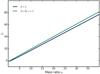 |
Fig. 1. Mass–radius exponent of the Roche radius (Eq. (25)) as a function of mass ratio q. The different colours denote different mass-loss modes. For the blue line the entire mass is transferred and re-emitted isotropically, while for the green line the entire transferred mass is accreted. |
The evolution of an SGXB where the donor star fills its Roche lobe depends on the mass–radius exponents. If ζR ≤ ζL, the Roche lobe shrinks faster than the star, which will overfill its Roche lobe even more, leading to a higher mass-transfer rate, and so on. This runaway process results in a CE evolution. If ζR > ζL, however, the donor radius is more sensitive to mass loss than the Roche radius, and the mass-transfer rate becomes self-regulated and can be estimated using the donor mass and its nuclear timescale as Ṁ ≈ M D/τ nuc (Soberman et al. 1997).
2.4. Binary evolution models
After investigating the mass–radius exponent of our single-star models, we selected those with high values of ζR. We added point-mass companions with 2 or 10 M⊙ and started the binary evolution. The initial orbital separation was selected such that the Roche radius exceeded the initial photospheric radius of the donor by 3%. We used the method described above to calculate the mass transfer and the accretion rate. We evolved the models with BEC until the hydrogen in the core of the donor star was exhausted or the mass-transfer rates exceeded ∼10−2 M⊙ yr−1, where we assumed that the mass transfer becomes dynamically unstable and the system enters a CE phase. Subsequently, we calculated the X-ray lifetime, defined as the time interval where the compact companion accretes at a higher rate than 10−13 M⊙ yr−1, which corresponds to an X-ray luminosity of ∼ 1033 erg s−1.
3. Results from single-star models
3.1. Response of the stellar radius
Here, we explore how the radii of our potential donor stars are affected by mass loss on a nuclear timescale. The resulting values of ζR can then be compared to the functions ζL plotted in Fig. 1 to obtain an estimate for which mass ratios we can expect stable mass transfer.
Figure 2 shows the mass–radius exponent ζR of our 60 M⊙ model evolved to a central helium mass fraction of Yc = 0.8. At the start of our mass-loss experiment, the model has a mass of 51 M⊙, a convective core of ∼32 M⊙, and a H/He gradient of about  in the core-envelope transition zone.
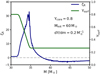 |
Fig. 2. Mass–radius exponent (blue) of our initial 60 M⊙ model evolved to a central helium abundance of 0.8, and a H/He gradient of |

We stripped the mass through a constant mass-loss rate of 10−5 M⊙ yr−1. As explained above, this rate is sufficiently low to maintain thermal equilibrium inside the model. Figure 2 shows that with decreasing stellar mass, the mass–radius exponent is low and negative at first because the stellar luminosity-to-mass ratio decreases. However, when He-enriched layers approach the surface, the mass–radius exponent climbs to values of 30, before it drops again to a low value when the stellar core is exposed. A value of ζD = 30 implies that a mass decrease by 1% induced the radius of the star to decrease by 30%. According to Fig. 1, such high values of ζD could give rise to a phase of stable mass transfer even for mass ratios as high as 15.
The drastic shrinkage of our models is related to the transition from a hydrogen-rich supergiant stage, with a radius of about 68 R⊙, to a much more compact and hydrogen-poor Wolf–Rayet-type structure with 6 R⊙. This is eminent from the correlation of the mass–radius exponent with the change in surface helium abundance, as shown in Fig. 2. Here, we note that the mass–radius exponent changes sign and evolves to high values somewhat before helium-enriched layers reach the surface of the star because the average envelope properties determine its radius. This is in agreement with previous stellar structure and evolution calculations (e.g. Köhler et al. 2015; Schootemeijer & Langer 2018).
Figure 3 shows that the internal H/He gradient is a suitable way to tune the mass–radius exponent ζD in our models. It depicts the result of the same experiment as explained above, but for six models with different steepness of the H/He-gradient. The models with steeper gradients reach higher values of ζD, even exceeding ζD = 40 in the most extreme case. While this may appear surprising at first because such high values of the mass–radius exponent have not yet been reported in the literature, it is a simple consequence of the mass in the transition layer between the He-rich core and the H-rich envelope, ΔMH/He, becoming very low for a steep internal H/He gradient, and ζD ≃ (RH − RHe)M/(RHeΔMH/He) becoming higher the lower ΔMH/He → 0. Here, RH is the stellar radius in the H-rich state, and RHe is the radius in the He-rich state, while M is the mass of the star.
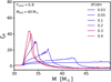 |
Fig. 3. Mass–radius exponent of our initial 60 M⊙ model in the same way as for the blue line in Fig. 2, but here for models where the internal helium gradient dY/dm has been artificially adjusted (see Sect. 2) to values indicated in the legend. |
Infinite H/He gradients, although not strictly excluded, are not expected in massive stars. However, it is important to point out that the range in steepness explored in Fig. 3 remains well within the range that has been derived by Schootemeijer & Langer (2018) from the observed properties of the WN-type Wolf–Rayet stars in the SMC. As we discuss in Sect. 5 below, this group of stars is quite relevant here because SGXBs may evolve into WN-type Wolf–Rayet binaries.
The mass–radius exponents of all our single-star models (50 M⊙, 60 M⊙, and 80 M⊙) and core helium abundances (0.6, 0.7, 0.8) are shown in the appendix (Figs. A.1–A.3), where we explore six different H/He gradients per models, as in Fig. 3. These figures show that in addition to the clear correlation between the mass–radius exponent and the helium gradient, higher mass–radius exponents are also obtained for a higher initial mass and for a later evolutionary stage (larger core helium mass fraction). Figure 4 summarises these results by showing the maximum value of the mass–radius exponent ζR as a function of the adopted internal helium gradient dY/dm for all our single-star models.
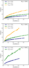 |
Fig. 4. Maximum value of the mass–radius exponent ζR as a function of the chosen internal helium gradient dY/dm for stellar models derived from three different initial masses as indicated in the legends. Different colours indicate different core helium abundances at the start of the mass-loss experiments (see Sect. 2). |
3.2. Influence of stellar inflation
In their analysis of the massive single star evolutionary models for LMC composition of Brott et al. (2011), Köhler et al. (2015), and Sanyal et al. (2015) found that the envelopes of models for stars above ∼40 M⊙ are inflated because they exceed the Eddington-limit in their subsurface layers. Whether such inflated envelopes (see Fig. 5, e.g.) exist in reality is still a matter of debate, although they have been confirmed by 3D radiation-hydrodynamic calculations (Jiang et al. 2015).
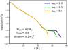 |
Fig. 5. Mass density as function of radius for our initially 60 M⊙ models with Ycore = 0.8 and |

The mass of the inflated envelope is mostly very low, that is, about 10−6 M⊙ in our models. However, its radius may be of the order of the radius of the un-inflated stellar interior. Obviously, radius inflation may play a great role in binary evolution. It is therefore important to analyse how inflation may affect the mass–radius exponent.
For this purpose, we investigated our 60 M⊙ single-star model at a core helium mass fraction of Ycore = 0.8 and  , from which we constructed three different initial models for our mass-loss experiment. The only difference in these models is the chosen mixing length parameter αML = l/HP, were l denotes the mixing length and HP the pressure scale height (cf. Sect. 2). We computed models with values for αML of 1 (our default choice), 1.5, and 50. Whereas the first two values are in the range discussed in comparison to 3D models of convection and real stars (Sonoi et al. 2019), we used αML = 50 to produce a stellar model in which inflation is suppressed but not absent (cf. Sanyal et al. 2015).
The mass–radius exponents of these three models are plotted in Fig. 6. We find that stellar inflation has a significant effect on ζR. While for strong inflation (αML = 1) the maximum value of ζR reaches 34, it only reaches 21 when inflation is suppressed (αML = 50). We also note that the value of the mass–radius exponent is initally more negative for the inflated models. However, the high peak of ζR occurs only when a H/He gradient appears beneath the surface.
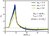 |
Fig. 6. Mass–radius exponent as function of stellar mass, with the three models displayed in Fig. 5 as initial models before assuming a constant mass-loss rate of 10−5 M⊙ yr−1. The colours correspond to the density profiles in Fig. 5. |
In Fig. 7 we compare the radius extension of the un-inflated part with that of the inflated envelope layer during the mass-loss experiment for our three models. Here, we followed Sanyal et al. (2015) to define the bottom of the inflated envelope as the point where the gas–pressure contribution Pgas/(Pgas + Prad) drops to 15% for the first time when going from the stellar center outwards. We refer to this position as R15. As the gas–pressure fraction in our model computed with αML = 50 never drops below 15%, we define the radius R30 as the position where the gas–pressure fraction first drops below 30%. The near coincidence of these two radii in the top and middle panel of Fig. 7 suggest that the exact threshold value of the gas–pressure fraction in defining the bottom of the inflated envelop is not important.
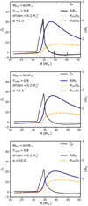 |
Fig. 7. Mass–radius exponent ζR (grey), stellar radius R (blue), and radii where the gas pressure contributes only 15% (R15) and 30% (R30) to the total pressure (see text), as function of the remaining stellar mass for the three models with different values of the mixing length parameter αML shown in Fig. 6 (the lines for ζR are identical). All radii are measured in units of the initial stellar radii R0, which can be read off Fig. 5. |
Figure 7 shows that before the helium gradient appears beneath the stellar surface (cf. Fig. 2), the stellar radius expands significantly as a result of inflation. This effect is stronger in the model computed with lower αML because the radius of the un-inflated part of the star (defined through R15 and R30 in Fig. 7) behaves in the same way in all three cases.
All three models have the same final configuration after they are stripped down to the helium core, therefore Fig. 7 offers a simple explanation of the dependence of the maximum of the mass–radius exponent on the mixing length parameter found in Fig. 6 because inflation is a much smaller effect for hot and compact models (Sanyal et al. 2015). For smaller αML, the hydrogen-rich models are more extended, and the drop in radius towards the compact stage is thus stronger than when αML is larger. We conclude that inflation is not a critical factor in producing high mass–radius exponents, but that it can contribute at the quantitative level, that is, it can enhance the mass–radius exponent by factors of the order of 2 for stars that exceed the Eddington limit.
4. Binary evolution models for SGXBs
In the previous section, we found that models of supergiant stars may show very high mass–radius exponents, with values up to ∼40. When we compare these to the mass–radius exponents of the Roche radius in Fig. 1, we expect that mass transfer on nuclear timescales may occur even in binaries with mass ratios of 20 or higher. To demonstrate this, we constructed appropriate initial models and combined them with point masses in model binary systems. We then calculated the detailed binary evolution of such systems with our binary evolution code (BEC).
We drew our initial models for these calculations from our 60 M⊙ models with a central helium mass fraction of Ycore = 0.8, from which we took one model with a rather shallow helium gradient ( ) and a second one with a helium gradient that was ten times steeper (
 ). The helium profiles of these two models are shown in Fig. 8. We note that a helium gradient of
  corresponds to the gradient that is left by the retreating convective core during core hydrogen burning, whereas a gradient that is steeper by about ten times can be established above the helium core during hydrogen shell burning, as derived for the SMC Wolf–Rayet stars by Schootemeijer & Langer (2018).
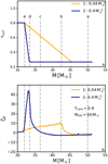 |
Fig. 8. Top panel: helium surface abundance as function of the total mass of the two stellar models from which the initial donor star models for our binary evolution calculations are derived. They are constructed such that mass located above the lines labelled a to e was removed before the binary calculation was started. Bottom panel: mass–radius exponent for the models as a function of the remaining stellar mass. Dashed lines correspond to the masses (labels a to e) in the upper panel. |
From each of these two models, we constructed five different initial models to calculate the binary evolution by removing the envelope mass down to the mass indicated by labels a to e in the top panel of Fig. 8. The choice of these amounts of removed envelope mass becomes clear from the bottom panel of Fig. 8, which shows the mass–radius exponent of the two models as a function of the remaining mass. It indicates that with the chosen envelope masses, our binary evolution models sample the possible range of the initial mass–radius exponent of the donor star.
For each of the ten initial donor star models described above, we performed several binary evolution calculations. We considered two different compact objects, a 2 M⊙ NS and a 10 M⊙ BH. Furthermore, we ran models with different assumptions on the donor star’s stellar wind mass loss, that is, without wind, with a constant stellar wind mass-loss rate, and with the mass-loss rate according to the prescription of Vink et al. (2001). Table B.1 gives an overview of the different binary evolution models, the details of the initial donor star models, and key quantities describing the evolution of the model binaries.
For the following discussion, we label the initial donor star models depending on their initial mass (using letters a to e according to Fig. 8), and numbers 1 or 2 depending on their helium gradient. For instance, model a1 refers to the initial donor star model with a helium slope of  (orange curve in Fig. 8) and an initial mass of 50 M⊙, while model e2 has
  (blue curve in Fig. 8) and an initial mass of 32 M⊙.
We further label the binary evolution models by indicating whether the accretor is a 10 M⊙ BH or a 2 M⊙ NS, using two letters (bh or ns). Finally, we indicate whether the donor star undergoes no mass-loss (0), mass loss with a constant rate of 10−6 M⊙ yr−1 (c), or time-dependent mass loss according to Vink et al. (2001)(v). For instance, the binary model d2ns0 consists of the initial donor model d2 as defined above and an NS accretor. During the binary evolution, the donor loses no mass through stellar wind.
4.1. Detailed example: Donor model d2 with a neutron star companion
Here, we discuss one of our binary evolution models in detail. For this we chose model d2 as donor star, which we placed together with a 2 M⊙ NS in an orbit of 9.1 d. The initial mass ratio in this binary is 16.8, such that highly unstable mass transfer might be expected. However, the envelope mass of model d2 was chosen such that the steep helium gradient in the initial donor model is located just beneath the surface, such that we expect an initial mass–radius exponent of ζR ≃ 40 in this case (Fig. 8).
Figure 9 shows the evolution of the mass-transfer rate as function of time for this model, where stellar wind mass loss is neglected. It shows that after a brief switch-on phase (∼104 yr), the model establishes a rather stationary mass-transfer rate of 3 × 10⁻⁶ M⊙ yr−1, which is maintained for ∼250 000 yr. During this time, the orbital period decreased from 9.1 d to 1.4 d. This was possible without leading to a CE situation because the donor star radius shrank from 36 R⊙ to 10 R⊙ at the same time. This shrinking of the donor star was enabled by the continuously increasing surface helium abundance during the mass transfer (Fig. 9): the donor star starts the mass-transfer phase as an early B-type supergiant (Teff ≃ 25 kK) and ends it as a late-type WNh star (Teff ≃ 50 kK).
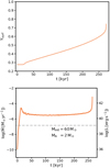 |
Fig. 9. Evolutionary properties of our model d2ns0, neglecting a 2 M⊙ NS companion and stellar winds. Top panel: surface helium mass fraction of the donor star as function of time during the mass-transfer phase. Bottom panel: evolution of the mass-transfer rate for the same model (left Y-axis). The right axis indicates the X-ray luminosity corresponding to the mass-transfer rate (not Eddington limited) assuming an accretion efficiency of η = 0.15. The dashed line gives the Eddington accretion limit for the NS that is applied in this calculation. Despite the high initial mass ratio of 16.8, the model settles into a stable mass transfer for about 0.25 Myr, with a mass-transfer rate of about the rate of the mass transfer on a nuclear timescale. |
Figure 9 also gives an indication of the X-ray luminosity that might be expected from binaries similar to our system d2ns0. In the evolutionary calculations, we assumed Eddington-limited accretion onto the NS, which would produce an X-ray luminosity of the order of 1039 erg s−1 (dashed horizontal line), comparable to what is found in some SGXBs. However, Fig. 9 also shows that if the NS could accrete at super-Eddington rates, X-rays of up to 1041 erg s−1 could be achieved. We discuss this possibility further in Sect. 5.1.
The mass transfer lasts for about 0.25 Myr with a mass-transfer rate of 3 × 10⁻⁶ M⊙ yr−1, which is two orders of magnitude above the Eddington limit of 3.6 × 10⁻⁸ M⊙ yr−1 of an NS and corresponds to an accretion luminosity 2.5 × 1040 erg s−1 (Fig. 9). The orbital period decreases from nine days to one day. Because the mass-transfer rate is much higher than the Eddington-accretion limit, most of the transferred mass in this calculation is re-emitted. According to Eq. (15), the orbital separation shrinks exponentially with the mass ratio. Because q ∝ MD and ṀRLO is roughly constant during most of the mass-transfer phase, the orbital separation also shrinks exponentially with respect to time.
During the mass transfer, about 1.5 M⊙ are removed. Figure 10 shows the evolution of the donor star during the mass-transfer phase in the Hertzsprung–Russel diagram. The evolutionary track starts at Teff ≃ 25 kK). As discussed before, the donor star becomes hotter and slightly more luminous during the mass-transfer phase. Its temperature remains for the longest time between 25 and 40 kK, which coincides with the regime where SGXB donor stars are observed (cf. Sect. 6.1).
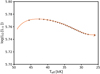 |
Fig. 10. Hertzsprung–Russel diagram for the donor star of binary model d2ns0. Black dots correspond to time differences of 104 yr. |
The connection of increasing surface helium abundance and increasing effective temperature has been recognized before by Brott (2011) and Köhler et al. (2015) for the evolution of massive single stars. In the cited works, the increasing surface helium abundance was due to rotational mixing and strong wind mass loss. Therefore only massive stellar models (> 60 M⊙) with high rotational velocities evolved to the hot part of the Hertzsprung–Russel diagram during core hydrogen burning.
4.2. Models without stellar winds
We first discuss the binary models with a a shallow helium gradient of  , neglecting stellar wind mass loss. Figure B.2 shows the evolution of mass-transfer rate, orbital period, and donor mass with time for binary models a1bh0, b1bh0, c1bh0, d1bh0, and e1bh0. Of these, models b1bh0 and c1bh0 undergo an extended phase of mass transfer of 0.5 Myr and 0.15 Myr, respectively. Despite the rather high mass ratio of q ≃ 4, this is much longer than the thermal timescale of the donor star (∼104 yr).
Figure B.2 also shows the X-ray luminosity corresponding to the mass-transfer rate, assuming an accretion efficiency of a non-rotating BH (η = 0.06). Because the accretion rate might be Eddington limited, this shows the highest achievable X-ray luminosity, where realistic values are expected between this and the value corresponding to the Eddington-accretion rate for a non-rotating BH. For super-Eddington accretion in these systems, a luminosity up to ∼ 1040 erg s−1 could be achieved. This matches the order of magnitude of X-ray luminosities that are observed in ultra-luminous X-ray sources. We note that our models do not only show a high mass-transfer rate, but also a long X-ray lifetime.
It is a remarkable feature of the two binary models b1bh0 and c1bh0 that the mass-transfer rate increases steeply after some hundred thousand years. This occurs at the time where the flat inner part of the helium profile (Y(m) = 0.8; cf. Fig. 8) reaches the surface, supporting the idea that a steep H/He gradient is needed to stabilise the mass transfer. As soon as the helium profile close to the surface is flat again, the mass transfer becomes unstable, as expected for a high mass ratio.
Why do only models b1bh0 and c1bh0 show a long-term mass transfer? As shown by Fig. 8, the donor star of model a1bh0 contains a massive hydrogen-rich envelope. The companion has to remove about 5 M⊙ to dig out the H/He transition layer. By doing so, the orbit shrinks dramatically (cf. Table B.1). When we assume that most of the transferred mass is re-emitted, we indeed find according to Eq. (15) that a/a0 = 0.42. This means that the orbital separation and hence the donor radius halve even before the helium gradient scratches the surface.
The mass transfer in models d1bh0 and e1bh0, on the other hand, is not long-term stable because the donor star has already lost so much mass that the helium-rich plateau is close to or even at the surface at the beginning of mass transfer, as is shown in Fig. 8. The donor star in model d1bh0 needs to lose only 1 M⊙ to find the flat helium profile in its outer envelope. For a mass-transfer rate on a nuclear timescale of 2 × 10⁻⁵ M⊙ (Fig. B.2), it would take only ∼50 000 yr to remove this layer. This is of the order of the thermal timescale. This means that mass-transfer on a nuclear timescale can hardly be distinguished from a from a runaway mass-transfer on a thermal timescale.
The evolution of donor models a1 and e1 are also shown, including an NS companion in Fig. B.1. None of these binary models undergoes mass transfer on a nuclear timescale. This is expected because Fig. 8 suggests a maximum mass–radius exponent of ζR ∼ 10. Because the initial mass ratio is ∼20, we find according to Fig. 1ζL ∼ 30 and thereby ζR < ζL. The Roche radius is more sensitive to mass transfers than the donor radius, therefore a runaway on a thermal timescale is unavoidable. Thus, the mass transfer for donor models a1ns0 and e1ns0 is not sufficiently stabilised by the helium gradient to allow an evolution on a nuclear timescale.
However, our models with a steeper H/He gradient can lead to mass transfer on a nuclear timescale in the case of an NS accretor as well, as we showed in Sect. 4.1. Figure B.1 displays the evolution of the mass-transfer rate for our models a2ns0 to e2ns0, which differ from models a1ns0 to e1ns0 only in the slope of the helium gradient. We see that model d2ns0 alone undergoes mass transfer on a nuclear timescale because the mass ratio is more extreme than in the case of BH accretors. Still, for NS accretors, mass transfer on a nuclear timescale is also clearly possible if the outer envelope of the donor star has a steep H/He gradient.
Finally, Fig. B.2 shows the mass-transfer rates and corresponding luminosities of our binary models that are composed of a donor with a steep H/He gradient ( ) and a 10 M⊙ BH companion (models a2bh0 to e2bh0). Similar to the case of donors with the shallower H/He gradient, only models c2bh0 and d2bh0 develop mass transfer on a nuclear timescale. However, because of the higher mass–radius exponents of models c2bh0 and d2bh0, the mass-transfer rates remain somewhat lower. Because of this, and because the initial donor radii of models c2bh0 and d2bh0 are somewhat larger than those of models c1bh0 and d1bh0, the mass transfer lasts for about 650 000 yr in both cases.
Both donor stars start to contract towards core helium ignition, such that the mass-transfer rate drops, and we end our calculations. We consider the further evolution of our systems qualitatively in Sect. 7.
4.3. Models including stellar winds
We showed that our binary models may undergo long-term mass transfer if the H/He transition layer of the donor star is close to the surface. Furthermore, in order to obtain mass transfer on a nuclear timescale, the H/He gradient needs to be steeper for NS accretors than for BH accretors because of the more extreme mass ratio in the former. Here, we debate the question whether an additional mass loss due to a stellar wind mass from the donor star could have an additional, perhaps stabilising, effect. To investigate this, we performed the same binary calculations as in the previous subsection, but with an additional constant donor wind mass-loss rate of 10−6 M⊙ yr−1, or, alternatively, with the mass-loss rate as given by Vink et al. (2001). We restrict these calculations to the donor star models that include the steep H/He gradient (donor models a2 to d2).
We start our discussion with the binaries that host a BH accretor (Fig. B.2). Comparing the calculations that include the two wind recipes to those without any wind, we find that they differ only slightly in the case of a constant mass-loss rate. The most import difference here is that the mass-transfer rate does not exceed the Eddington-accretion limit in the late phase of mass transfer when a wind is included. The X-ray lifetime as well as the orbital separation do not change very much compared to Fig. B.2. This is to be expected because the wind mass-loss rate of 10−6 M⊙ yr−1 is comparable to the mass-transfer rate in this case.
The situation is different when we include Vink’s mass-loss scheme. The predicted mass-loss rates are higher by an order of magnitude than the constant mass-loss rate discussed before (Ṁw ∼ 10−5 M⊙ yr−1), as shown with the dotted line in Fig. B.2. Vink’s wind mass-loss rate in our models is of the same order or even higher than the mass-transfer rate on a nuclear timescale for the corresponding binary models that are inferred without any stellar wind. This means that the donor star can shrink only due to its own wind mass loss. Mass transfer does not occur on a nuclear timescale because the Roche-lobe overflow is no longer self-regulated. In one case (model d2bhv), Roche-lobe overflow is not even initiated because the donor avoids any expansion. As discussed above, any stellar wind will expand the orbital separation. The fast-shrinking donor radius and the expanding orbital separation drive the systems far away from Roche-lobe filling. On the other hand, when the hydrogen-rich envelope is not yet removed or when the former convective core with a flat helium gradient is already at the surface, the radius is no longer sensitive enough to mass loss. In theses cases, even a strong stellar wind does not help to maintain a stable system.
In the case of NS accretors, we find that a donor wind could have a substantially stabilising effect. This is shown in the example of model d2bhc in Fig. B.1, for which a constant mass-loss rate of 10−6 M⊙ yr−1 extends the mass-transfer phase from 250 kyr in case of no wind to more than 600 kyr. However, a higher stellar wind mass-loss rate can have the opposite effect here as well. Model d2bhv does not undergo Roche-lobe overflow. The reason is that model d2 is the donor model with the highest ζR (cf. Fig. 8). In the definition of the mass–radius exponent (Eq. (6)), the timescale of radius change reads τ = R/Ṙ as  . When the Vink mass-loss recipe is applied, the mass-loss timescales is of the order of the nuclear timescale. Because ζR ∼ 30 for donor model d2, the timescale for radial changes is much shorter than the nuclear timescale. This means that changes in donor radius are due to the intrinsic mass loss, which decreases the radius in our models, and not to nuclear processes, which would expand the star. This results in a rapid radial shrinking of the donor star even before mass transfer is initiated. When ζR is smaller (models a2, b2, c2, and e2) or the mass-loss timescale is longer than the nuclear timescale, which is the case when the constant mass-loss rate is applied, the nuclear evolution of the donor star can increase the radius initially and thus initiate the mass transfer.
We conclude that the donor star winds may play an important role in determining the duration of the mass-transfer phase and thus the X-ray lifetime of SGXBs, which they may extend or decrease. We emphasise that the mass-loss rates of helium-enriched OB supergiants are uncertain by more than a factor of two (Ramírez-Agudelo et al. 2017). In addition, wind clumping (El Mellah et al. 2018) and X-ray emission in SGXBs may affect the donor star wind (e.g. Sander et al. 2018). A more detailed study of the influence of the donor wind on the SGXB evolution is therefore clearly warranted, but is beyond the scope of our present paper.
4.4. Orbital period derivatives
As discussed in Sect. 2.3, mass transfer induces changes in orbital separation. These changes may be observed as changes in orbital period. To show the effect of mass transfer due to Roche-lobe overflow on the orbital period, we derive expressions for the orbital period derivative for the case of pure isotropic re-emission ( β = 1), and for conservative mass transfer (ϵ = 1). Equations (15) and 16 describe the change in orbital separation for these cases.
The derivative of Kepler’s third law with respect to time leads to
When the change of orbital separation is expressed as a/a0 = f(q), as in Eqs. (15) and 16, then

With Ṁ = Ṁ1 for the case of isotropic re-emission, we find
and with Ṁ = 0 for conservative mass transfer,
For both cases, that is, from Eqs. (29) and (30), a high mass ratio (q ≫ 1) implies

Thus, we expect the orbital period derivative for mass transfer driven by Roche-lobe overflow to be essentially independent of the accretion rate of the compact object, as long as the mass ratio is high. Furthermore, Ṁ1 < 0 implies a decrease in orbital period during mass transfer, regardless of how conservative the mass transfer is. Hence, isotropic re-emission and conservative mass transfer lead to an orbital decay at a very similar rate.
The orbital period of model d2ns0, with a donor mass of ∼30 M⊙ (Table B.1) and a mass-transfer rate of ∼3 × 10⁻⁶ M⊙ yr−1 (Fig. 9), decreases with Ṗ/P ≈ −4.5 × 10⁻⁶ yr−1 for either a BH or NS companion. For donor models c2bh0 and d2bh0 with BH companions (Fig. B.2), the orbital decay rate is about one order of magnitude lower, with Ṗ/P ≈ −6 × 10⁻⁷ yr−1. If the H/He gradient is shallower, as in model b1bh0 (Fig. 13), the orbital decay is faster by more than one order of magnitude (Ṗ/P ≈ −10−5 yr−1).
Falanga et al. (2015) compiled and evaluated the orbital period changes of ten eclipsing SGXBs from a multi-decade monitoring campaign. Five sources in their sample showed a significant change in orbital period. All of these five sources showed decaying orbits (Ṗ/P < 0), with rates |Ṗ/P| ∼ 1 … 3 × 10⁻⁶ yr−1. The source EXO 1722-363 shows an orbital decay rate of Ṗ/P = (−21 ± 14) × 10−6 yr−1. Although the uncertainty is smaller than the measured value, Falanga et al. (2015) did not label this source as significant. We note that the orbital decay rate is consistent with zero within the 2σ error. For four more sources, no orbital decay within the 1σ environment was observed. We used the 1σ uncertainty provided by Falanga et al. (2015) as an upper limit for the orbital decay rate.
In Fig. 11 we compare the empirical values with the Ṗ/P-evolution of our model d2ns0 with an NS accretor together with our analytic estimate for its period derivative. All five sources for which an orbital decay rate was measured with high significance are in good agreement with the decay rate of our model. This means that deviations between the theoretical model and the observed orbital decay rate are not much larger than a factor of two (the time coordinate for the empirical values in Fig. 11 has no meaning). This is remarkable because our models were not tailored to reproduce the observed sources.
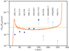 |
Fig. 11. Evolution of the orbital period derivative Ṗ/P of our model d2ns0 shown in Fig. 9 as given by the numerical simulation (orange line), together with our analytic estimate for the same model (see text; yellow line). Overplotted are the empirical decay rates of ten SGXBs as inferred by Falanga et al. (2015), who give six measured values with 1σ error bars (blue dots; for most of these, the error bar is smaller than the size of the dot) and four upper limits (blue arrows). We note that the time axis has no meaning for the period derivatives of the observed sources. |
The only source that does not fit our model well is Vela X-1. The upper limit of the decay rate lies one order of magnitude below our prediction. Equation (29) suggests that the mass-transfer rate must not exceed a few times 10−7 yr−1 in order to obtain a decay rate below the upper observation limit. We did not find such low mass-transfer rates in our models with NS accretors. We therefore conclude that the orbital change of Vela X-1 is at least not modelled with our simple prescription. This does not completely rule out Roche-lobe overflow as a possible accretion mode for this source. The low orbital decay rate may be explained if Vela X-1 were just in a transition state between wind-dominated accretion and atmospheric Roche-lobe overflow.
We note that orbital decay may be more complex than discussed in this section. In our simplified description, effects such as tidal interaction (Lecar et al. 1976; van der Klis & Bonnet-Bidaud 1984; Safi Harb et al. 1996; Levine et al. 2000) or the Darwin instability (Lai et al. 1994) are neglected. These mechanisms may also be able to drive orbital decay that is in agreement with the observed decay rates (Kelley et al. 1983; van der Klis & Bonnet-Bidaud 1984; Levine et al. 1993; Rubin et al. 1996; Safi Harb et al. 1996; Jenke et al. 2012). In any case, our calculations show that the observed orbital decay rates of SGXBs may be explained by the simple isotropic re-emission model as long as the mass transfer occurs on the nuclear timescale. The fact that highly non-conservative and conservative mass transfer show the same orbital decay rates for high mass ratios implies that SGXBs and ULXs should show similar values of Ṗ/P within this prescription.
5. Binary evolution models for ULXs
The Eddington luminosity of a 10 M⊙ BH is about 3 × 1039 erg s−1. Brighter X-ray sources are considered ultra-luminous X-ray sources (ULXs). As the mass-transfer rates on nuclear timescales in our models are in the range 10−5…10−6 M⊙ yr−1, some of them might be considered as models for ULXs with up to ∼1041 erg s−1 (cf. Table B.1) if the entire transferred matter were accreted.
5.1. ULXs with neutron star
It has recently been discovered that several ULXs show X-ray pulsations, which is only expected if the compact accretor is an NS (Kaaret et al. 2017). While the Eddington limit of NSs is well below 1039 erg s−1, some of the X-ray pulsating ULXs show X-ray luminosities that are clearly in the ULX regime (Bachetti et al. 2014). Whiles beaming effects might help to explain the very high X-ray luminosities (King 2001), some NSs in ULXs have been shown to experience an extreme spin-up on a short timescale, which may require actual accretion onto the NS at rates much above the classical Eddington limit (Israel et al. 2017a, but see King & Lasota 2019). One way to understand such high luminosities from accreting NSs is to invoke magnetic fields with a field strength above ∼1013 G, which could reduce the radiative opacity of the accreted matter and thus raise the Eddington limit (Herold 1979; Ekşi et al. 2015; Israel et al. 2017a).
It has also been suggested that ULXs that host NSs might host intermediate-mass donor stars (Karino 2016). However, Tauris et al. (2017) argued that corresponding models only work for donor star masses below 7 M⊙. The donor star in the ULX pulsar in NGC 5907 is constrained to be higher than ∼10 M⊙, and its orbital period is found to be  d (Israel et al. 2017a). Motch et al. (2014) determined the orbital period of the ULX pulsator NGC 7793 P13 to ∼64 d, where the mass donor is a B9Ia supergiant of about 20 M⊙ (Israel et al. 2017b). Except for being ultra-luminous, their parameters are reminiscent of those of the SGXBs.
Our model d2ns0 in Sect. 4.1 obtains a mass-transfer phase on nuclear timescales, with accretion rates that would lead to X-ray luminosities above 1040 erg s−1 if the NS could accrete all the matter. In order to probe this situation, we repeated the calculation displayed in Fig. 9, but allowed the NS to accrete the entire transferred matter. While this may not be realistic because a fraction of the transferred matter may always be expelled, it provides the limiting case, with more realistic models bounded by this and the Eddington-limited calculations shown in Sect. 4.1.
Figure 12 shows that the long duration of the X-ray bright mass-transfer phase is not only maintained by the conservative accretion model, but the time span of X-ray emission is almost doubled compared to the Eddington limited model. This is understandable because the mass of the NS grows significantly here, it would likely eventually collapse into a BH, as a total of about 1.4 M⊙ is transferred, and the thus-reduced mass ratio leads to slightly lower mass transfer rates. However, its X-ray luminosity could still be well over 1040 erg s−1 for more than 400 000 yr.
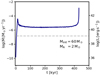 |
Fig. 12. Evolution of the mass-transfer rate for the same model as shown in Fig. 9 (left Y-axis) (Model d2ns0), but here calculated assuming conservative mass transfer. |
Our models do not attempt to reproduce any of the observed ULXs. However, they show that ULXs with NS accretors may accrete from Roche-lobe overflow for much longer than a thermal timescale of the donor star if their donor star is a helium-enriched supergiant.
5.2. Black-hole companions
Clearly, ULXs can form in binaries when one component is a sufficiently massive BH and the companion transfers mass at a high enough rate. In this situation, it has been recognised that beaming (King 2001; Körding et al. 2002), photon-bubbles (Begelman 2002; Ruszkowski & Begelman 2003), or magnetic accretion disc coronae (Socrates & Davis 2006) could help to raise the apparent or true Eddington limit, such that ULXs of up to 1041 erg s−1 can be explained with stellar mass BHs (Madhusudhan et al. 2008; Marchant et al. 2017).
In order to obtain non-negligible ULX lifetimes, the donor star in these models is usually of comparable or smaller mass than the BH, which severely limits the expected number of ULXs. In our models with helium-enriched donor stars, this restriction can be dropped. Assuming a 10 M⊙ BH, the initial mass ratio expected in such systems is significantly lower than in the case of an NS companion. Consequently, we find mass transfer on a nuclear timescale in more system when a BH is assumed to be present. In Fig. 13 we highlight our models b1bh0 with a donor star of initially 42.5 M⊙, which provides a high mass-transfer rate to an initially 10 M⊙ BH for almost 0.5 Myr, and which could provide an X-ray luminosity of ∼1041 erg s−1 when super-Eddington accretion is assumed.
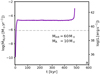 |
Fig. 13. Evolution of the mass-transfer rate as function of time for our model b1bh0, which starts with a 42.5 M⊙ supergiant and a 10 M⊙ BH in an 18 d orbit. |
In our models with NS accretors, only donor stars with steep H/He gradients led to Roche-lobe overflow phases on nuclear timescales. The mass ratio in systems with 10 M⊙ BH accretors is lower by five times, which leads to a slower shrinking of the orbit. Therefore even the ten times shallower H/He gradient is sufficient to achieve Roche-lobe overflow on nuclear timescales in these systems. This significantly may widen the parameter space for BH-ULX systems.
6. Implications for the origin of SGXBs
The way in which the donor stars of our supergiant and ULX binary models have been set up may raise doubts whether they are applicable for interpreting the observed systems. In particular, we have shown that mass transfer on a nuclear timescale was only achieved when the chemically homogeneous part of the hydrogen-rich envelop was removed before the mass transfer to the compact companion starts. This raises the question whether this may occur in reality.
6.1. Clues from observations
The first idea, that is, that the H/He transition layer is close to the surface of the donor star, appears to be supported by several observations. Using the data of Conti (1978) and Falanga et al. (2015), who determined the effective temperatures and surface gravities of several SGXB donors, we can compare the observed donor stars with stellar models in a spectroscopic Hertzsprung–Russel diagram (Langer & Kudritzki 2014). In this diagram, the ordinate values are proportional to the luminosity-to-mass ratio of the stars. Figure 14 shows that the SGXBs do not match single-star tracks of the corresponding mass. This has already been noticed by Conti (1978). For instance, the donor star in Vela X-1 appears close to the 100 M⊙ track, while its mass, inferred from radial velocity measurements, is only ∼25 M⊙.
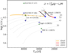 |
Fig. 14. Spectroscopic Hertzsprung–Russel diagram including data for SGXBs from Conti (1978; green crosses) and Falanga et al. (2015; blue crosses). The name of the source is added to the symbols. The parentheses include the donor masses as measured by Conti (1978) and Falanga et al. (2015). The grey dashed lines are tracks from single-star evolutionary models (Brott et al. 2011). The grey numbers indicate the initial mass of the corresponding stellar model. Red and orange lines indicate the evolution of our binary models. The starting point of each model is labelled with a blue star. The black dots correspond to time steps of 50 000 years. |
Because removing the stellar envelope decreases the mass but does not affect the luminosity significantly, it is not surprising that some of our SGXB models fit the spectroscopic Hertzsprung–Russel diagram position of Vela X-1 and other SGXB donors better than the single-star models. Figure 14 shows that model c2bh0 approaches the position of Vela X-1 near the end of its mass-transfer phase, where the mass of the donor star is about 33 M⊙ (cf. Table B.1), suggesting an initial donor mass closer to 60 M⊙. While Vela X-1 has no BH but an NS companion, this comparison shows that the luminosity-to-mass ratio (L/M) of our model may be close to that of the donor star in Vela X-1, implying that it did lose its hydrogen-rich envelope at an earlier stage of its evolution. Figure 14 shows that in all cases for which effective temperature and surface gravity could be determined, the corresponding L/M is well above that of the single-star models. This indicates that all the donor stars have already lost a significant portion, and perhaps all, of their non-enriched massive envelope.
Even more direct evidence for this comes from model atmosphere calculations and fits to observed donor star optical spectra of the SGXBs. An enhanced surface helium abundance was found in 4U 1700-377 (Clark et al. 2002), GX301-2 (Kaper et al. 2006), and Vela X-1 (Sander et al. 2018). A surface helium enrichment is expected to occur only after the chemically homogeneous non-enriched part of the stellar envelope is removed. The implication of the observed helium enrichments is that as a result of mass loss, whether by stellar winds or by Roche-lobe overflow, the donor star radii are currently decreasing. The remarkable circumstance that the donor stars in these systems are nevertheless very near Roche-lobe filling may imply that the orbit shrinks at the same time. This is only expected if the systems were currently undergoing Roche-lobe overflow. We conclude that SGXB observations provide ample evidence in support of the assumption that their donor stars have lost the non-enriched massive hydrogen envelope in a previous evolutionary phase.
We note that it is a consequence of the properties of the SGXBs we discussed that the initial mass of the NS progenitor in these systems must have been quite high, that is, higher than 30 to 40 M⊙. While BHs are generally expected to form from such massive stars, the presence of NSs in SGXBs could relate to the “island of explodability” at high mass that was found by Ugliano et al. (2012) and Sukhbold et al. (2016) in parametrised core-collapse explosion models. Brown et al. (2001) also suggested that stripped-envelope massive stars, that is, mass donors in close binary systems, tend to form NSs even for initial masses as high as 40 M⊙.
6.2. Clues from stellar models
The question to ask at this stage is through which mechanism the donor stars in SGXBs lost their H-rich envelopes before they entered the X-ray binary stage. As their initial masses appear all very high, it might be wondered whether the ordinary radiation-driven winds of massive stars are sufficient to reach this goal. Based on the massive star models in the literature (Smith 2014; Brott et al. 2011; Vink et al. 2001) and considering that the wind mass-loss rates for these very massive stars cannot be predicted to better than within a factor of ∼2 (with some of this coming from the metallicity spread in the Galaxy, e.g.), it may not be a problem to remove the required amounts of mass by stellar winds.
However, this mechanism would require a significant amount of fine-tuning. Because stellar wind mass loss always widens the orbits of binary stars (cf. Eq. (14) in Sect. 2.3), the expansion of the OB star needs to catch up with the increasing Roche radius at exactly the time when the H/He gradient appears near the stellar surface. Figure 1 shows that this is not impossible because the massive star models tend to increase in size as mass is being removed until shortly before helium-enriched layers appear at the stellar surface (see also Fig. 15 below). Only systems within a narrow initial period range would be able to fulfil the timing constraint, however.
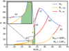 |
Fig. 15. Donor radius as a function of mass in thermal equilibrium (blue). The red lines show the Roche radius as a function of donor mass during the binary calculation that includes a 10 M⊙ accretor and no stellar wind of the donor. The yellow lines show the Roche radius after the binary calculation has stopped and CE is initiated. The orbital separation and hence the Roche radius was inferred using the energy budget description of CE. The green area marks the position of the H/He transition layer. |
The more common situation may be that the donor star fills its Roche radius at a time when the H/He-interface layer is still buried beneath a massive hydrogen-rich envelope. As we showed in Sect. 5, this leads to very high mass-transfer rates and likely to a CE evolution (see also Hjellming & Webbink (1987)). Here, the Roche-lobe overflow could start in the advanced phase of core hydrogen burning, or after core hydrogen exhaustion. While it is beyond the scope of this paper to comprehensively investigate the outcome of such an evolution, we provide a simple estimate as follows.
We show the radius evolution of our 60 M⊙ model (blue line), assuming mass loss on a nuclear timescale, in Fig. 15, together with the evolution of the Roche radius for our sequences a2bh0 to e2bh0 during the mass-transfer evolution (red lines). At the end of the mass-transfer evolution, a CE phase is expected. The yellow lines in Fig. 15 show the value of the donor Roche radius at a given donor star mass if the CE were removed at the corresponding time, where the Roche radius is obtained from equating the energy release ΔE from the decaying BH orbit with the envelope binding energy Ebin of the envelope above this orbit, where
and
is the effective binding energy, which includes gravitational binding energy reduced by the thermal energy. Here, MD, i is the donor star mass at the beginning of the CE evolution, MD is its mass at a putative end stage of the CE evolution, and ai and a are the corresponding orbital separations. The Roche radius during RLO was directly inferred from the binary calculation. At the point where the binary calculation stops, we used the last calculated donor model, orbital separation, and accretor mass to compute the Roche radius as function of the donor mass as described above. The stellar model of the donor at the beginning of the CE evolution defines the envelope binding energy Ebin as function of the remaining mass MD. The condition of Roche-lobe filling at the beginning of the CE evolution sets the orbital separation at that time for a given accretor mass. Assuming the accretor mass remains constant allows us to compute the Roche radius after the CE evolution as a function of donor mass MD at that time.
The evolution of our sequence a2bh0 in Fig. 15 provides a case where a merger appears to be the most likely outcome of the CE evolution. At its onset, the donor star mass is about 45 M⊙ and its H/He transition layer is buried beneath more than 10 M⊙ of hydrogen-rich envelope. At the same time, it is rather compact (RD ≃ 20 R⊙) because of its high mass-transfer rate. The yellow line for sequence a2bh0 in Fig. 15 shows that there is no possible final mass after the CE evolution for which the donor Roche radius would exceed its thermal equilibrium radius. While the donor radius may be smaller than its thermal equilibrium radius during mass transfer or immediately after a CE ejection, the implication is that if at all, it would be able to fit into its Roche radius only for a thermal timescale or less. Afterwards, it would expand and merge with the companion.
However, the picture is different for sequence b2, which is also expected to quickly undergo a CE evolution (cf. Fig. B.2). Figure 15 shows that in this case, the yellow line indicating the donor Roche radius crosses the blue line for the thermal equilibrium radius of the donor. Consequently, this model opens the possibility of a successful CE ejection at a time when the H/He-transition layer of the donor star is at the stellar surface. After this, the expectation is that the nuclear-timescale expansion of the donor would cause it to fill its Roche-lobe again soon, allowing mass transfer on a nuclear timescale onto the compact companion.
While our estimate in Fig. 15 includes many simplifications and is not to be understood as a quantitative model, it shows the interesting possibility that SGXBs can be interpreted as post-CE systems. In this frame, the emerging of the H/He transition layer at the donor surface at the end of the CE evolution is not a matter of fine-tuning, but is naturally produced by the sharp drop of its thermal equilibrium radius at this time. Potentially, all the models with initial masses in between those of sequences b2 and c2 could follow this path. The evolution of sequence b2 shows that in this scenario, a significant portion, or even the main portion, of the hydrogen-rich envelope may be transferred to the compact companion in a mass-transfer event on a thermal timescale before the onset of the CE evolution. The higher this fraction, the higher the chances to avoid a merger during the CE evolution.
We may point out that there are tentative observational counterparts for this type of evolution: the enigmatic X-ray binary SS 433 appears to have a supergiant mass donor that provides mass at the thermal mass-transfer rate (Fabrika 2004). Within our picture, SS 433 may qualitatively correspond to our models b2bh0 or c2bh0 at the time of the first mass-transfer peak (cf. Fig. B.2). It would then evolve into an ordinary SGXB after going through a CE phase (model b2bh0), or after avoiding a CE phase (model c2bh0).
Finally, our CE scenario for the pre-SGXB evolution may relate to the so-called obscured SGXBs that have recently been discovered (Chaty 2013). The ejected envelope may provide enough circumstellar material to produce the obscuration.
6.3. Metallicity dependence
We point out that the scenario for producing the SGXBs, either by well-timed stellar wind mass loss, such that it starts Roche-lobe overflow when the H/He transition layers appear at the surface, or through a pre-mass-transfer CE phase, may be favoured in a high-metallicity environment such as our Galaxy. This becomes clear when we compare the evolutionary tracks of massive single stars for solar metallicity with those computed with an initial composition as that in the SMC (Fig. 16). It shows that the first scenario does not appear to be available at low metallicity: While at solar metallicity, the models lose enough mass to expose their H/He transition layers without the help of a companion star, the low-metallicity models never do this.
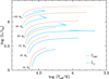 |
Fig. 16. Evolutionary tracks for solar and SMC metallicity during core hydrogen burning (Brott et al. 2011). |
In the Milky Way, Humphreys & Davidson (1979) found that the most massive stars avoid the upper right part of the Hertzsprung–Russel diagram. This has been related to the Eddington limit and the instabilities in the so-called luminous blue variables (Lamers & Fitzpatrick 1988; Ulmer & Fitzpatrick 1998; Gräfener et al. 2012; Sanyal et al. 2015). The proximity of the Galactic supergiants to the Eddington limit will therefore likely also facilitate the loss of the hydrogen-rich envelope when a compact companion is present. As a result of the iron opacity, the phenomenon is shifted to much higher luminosities and masses for low metallicities (Ulmer & Fitzpatrick 1998; Sanyal et al. 2017). Therefore, the mass of the hydrogen-rich envelop in SMC supergiants with compact companions, at the time they would likely fill their Roche-lobe, is likely much higher than in a comparable case in the Galaxy, and an immediate merger may be expected. While in the Milky Way, we have about as many SGXBs as BeXBs (Walter et al. 2015), only one SGXB is known in the SMC, but 81 confirmed BeXBs (Haberl & Sturm 2016). Our model may offer a natural explanation of this strong metallicity dependence.
A metallicity dependence would also be expected for the ULX application of our scenario. Our remarks about the donor stars in SGXBs also hold for ULX supergiant donors. This is particular relevant for ULXs with NS accretors because the mass ratio problem is the strongest in these sources. Consequently, we would preferentially expect ULXs with NSs at high metallicity. Our CE scenario may also have implications for understanding the generation of large-scale magnetic fields in stars. Based on the observation that magnetic white dwarfs are common in cataclysmic variables (CVs) but are absent in wide binaries (Wickramasinghe & Ferrario 2000) and Potter & Tout (2010) argued that the strong magnetic field in CVs with a magnetic white dwarf could be generated during their previous CE evolution. While their model appears only marginally successful, the idea may still apply. If it were transposable to massive X-ray binaries, it could imply that a CE phase in a pre-SGXB evolution may help to induce a strong field in the NS, with the effect of producing a ULX rather than an ordinary SGXB.
7. Evolution of SGXBs and SG-ULXs
We have ended our binary evolution calculations when either the mass-transfer rate exceeded ∼10−2 M⊙ yr−1, or when the models became thermally unstable as a result of core hydrogen exhaustion. Therefore, we can only conjecture about the further evolution of our model binaries and about the evolution of the observed SGXBs and SG-ULXs.
From the time dependence of the mass-transfer rates of our models, it can be concluded that after the H/He transition layer is lost during the nuclear-timescale evolution, the mass-transfer rate increases steeply. This is the case for our models b1bh0 and c1bh0 with BH accretors (Fig. B.2), and for model d2ns0 with an NS accretor (Fig. B.1), also for conservative mass transfer (Fig. 12). According to Hjellming & Webbink (1987), who inferred a maximum mass ratio of 2.14 for a binary to be stable against dynamical runaway, the onset of a CE evolution in these models appears likely. Because at this stage, our models are rather compact and still possess a significant envelope with a hydrogen mass fraction of 20%, we assume that a merger would be the likely outcome.
In another suite of our models, the mass transfer on a nuclear timescale lasts until hydrogen is exhausted in the core of the donor. The ensuing contraction of the donor model leads to a sharp drop of the mass-transfer rate, and the Roche-lobe overflow phase stops (model d2nsc, Fig. B.1, and models d2bh0 and d2bh0, Fig. B.2). We would expect that a hydrogen shell source will ignite in these models, which will expand their envelopes and initiate a mass transfer on a thermal timescale. Again, using the criterion of Hjellming & Webbink (1987), we would expect this to evolve into a CE phase, with a merger of both components as the result. Only two of our models with a time-dependant stellar winds (models b2bhv and c2bhvwith BH accretors) are expected to emerge as a Wolf–Rayet-BH binary.
However, our models are artificially constructed and are not self-consistently evolved from the zero-age main-sequence stage. For models a1 to e1, whose transition layer contains the shallower H/He gradient, the slope is naturally expected from the receding convective core during hydrogen burning. However, the steeper H/He gradient in models a2 to e2 is perhaps only formed after core hydrogen exhaustion (Schootemeijer & Langer 2018). In core helium burning supergiants, the mass transfer on a nuclear timescale might then stop at the time of core helium exhaustion. It may not be excluded that in this case, a merger during the short remaining time to the collapse of the donor star can be avoided, and a short-period double compact binary emerges.
A further investigation of the post-mass-transfer evolution of more self-consistent SGXBs and SG-ULXs clearly appears warranted.
8. Conclusions
We have refuted the long-standing paradigm that mass transfer in binary systems with a high mass ratio must be unstable and can last for at most a thermal timescale of the donor star. We first produced single-star models with mass radius exponents (e.g. Fig. 2) that far exceed those required for stable mass transfer in binaries with high mass ratios (Fig. 1). We then calculated detailed binary evolution models for SGXBs with NS and BH components, and found mass transfer on a nuclear timescale in many of them, with initial donor-to-accretor mass ratios of up to ∼20.
The key for the stability of the mass transfer in our models despite the inevitably strong orbital contraction is that their surface helium abundance is increasing. Thereby, the donor stars deflate their radius by a factor of a few during the mass transfer, and evolve from supergiants into Wolf–Rayet stars.
While our models are artificially constructed and not derived from earlier phases of binary evolution, their key feature appears to be supported by observations because the SGXB donors generally appear to be helium rich and overluminous for their mass (Fig. 14).
Furthermore, our models facilitate understanding several observations. The first is the large number of observed SGXBs in the Milky Way, which is proportional to the duration of their X-ray phase. The latter is drastically extended by our models. The second is the discovery of ULXs with supergiant donor stars and NS accretors. Again, in the standard picture, their lifetime is expected to be extremely short. We showed an example with an initial mass ratio of 17 and a ULX phase that due to stable Roche-lobe overflow lasted for more than 400 000 yr.
We argue that the SGXBs in the Milky Way, and perhaps also the ULXs with NS accretors, may have formed in a CE evolution, during which the loss of the H-rich envelope of the donor star was facilitated as it reached its Eddington limit. Such a CE phase might be related to the dense circumstellar medium found in the Galactic obscured SGXBs. While this could remove the fine-tuning problem of producing the SGXBs in their current state, it could also explain the nearly complete lack of SGXBs in the SMC, where stars reach their Eddington limit only at much higher mass.
If ULXs with NS accretors were to correspond to our CE scenario, they would preferentially be expected at high metallicity, and be rare at low metallicity, analogous to the SGXBs. ULXs with massive BH accretors, on the other hand, might have a preference for low metallicities, where the final BH masses are expected to be higher.
This scenario may also shed light on the question of how magnetar fields are created. It would make the ULXs with NS accretors, in which accretion rates of more than two orders of magnitude above the Eddington limit are thought to be enabled by extreme NS magnetic fields, the more massive cousins of polars, that is, CVs in which a main-sequence star sheds mass onto a magnetic white dwarf. These CVs are also thought to have undergone a previous CE evolution.
It is necessary to produce detailed progenitor models for SGXBs in order to validate the CE scenario. This may be useful as an understanding of the CE evolution of very massive stars as function of metallicity is also required to reliably predict the population of double BH binaries, into which some of the Galactic SGXBs might evolve. At the same time, there may be several avenues to provide stronger observational constraints to the CE evolution of very massive stars, including the search for binaries consisting of OB star and a BH or NS, many of which may have escaped detection so far.
Acknowledgments
We are grateful to Ed van den Heuvel and Philipp Podsiadlowski for useful comments and discussions. TMT acknowledges an AIAS-COFUND Senior Fellowship funded by the European Union’s Horizon 2020 Research and Innovation Programme (grant agreement no 754513) and the Aarhus University Research Foundation.
References
- Abbott, B. P., Abbott, R., Abbott, T. D., et al. 2016, Phys. Rev. Lett., 116, 061102 [Google Scholar]
- Abbott, B. P., Abbott, R., Abbott, T. D., et al. 2017, ApJ, 848, L12 [Google Scholar]
- Apparao, K. M. V. 1985, ApJ, 292, 257 [NASA ADS] [CrossRef] [Google Scholar]
- Bachetti, M., Harrison, F. A., Walton, D. J., et al. 2014, Nature, 514, 202 [NASA ADS] [CrossRef] [Google Scholar]
- Basko, M. M., Sunyaev, R. A., Hatchett, S., & McCray, R. 1977, ApJ, 215, 276 [NASA ADS] [CrossRef] [Google Scholar]
- Begelman, M. C. 2002, ApJ, 568, L97 [NASA ADS] [CrossRef] [Google Scholar]
- Bird, A. J., Malizia, A., Bazzano, A., et al. 2007, VizieR Online Data Catalog: II/170 [Google Scholar]
- Bird, A. J., Bazzano, A., Bassani, L., et al. 2010, ApJS, 186, 1 [NASA ADS] [CrossRef] [Google Scholar]
- Blondin, J. M., & Owen, M. P. 1997, ASP Conf. Ser., 121, 361 [NASA ADS] [Google Scholar]
- Böhm-Vitense, E. 1958, Z. Astrophys., 46, 108 [Google Scholar]
- Bondi, H., & Hoyle, F. 1944, MNRAS, 104, 273 [NASA ADS] [CrossRef] [Google Scholar]
- Bozzo, E., Oskinova, L., Feldmeier, A., & Falanga, M. 2016, A&A, 589, A102 [NASA ADS] [CrossRef] [EDP Sciences] [Google Scholar]
- Braun, H., & Langer, N. 1993, Space Sci. Rev., 66, 401 [NASA ADS] [CrossRef] [Google Scholar]
- Brott, I. 2011, PhD Thesis, Sterrrenkundig Instituut Utrech, The Netherlands [Google Scholar]
- Brott, I., de Mink, S. E., Cantiello, M., et al. 2011, A&A, 530, A115 [NASA ADS] [CrossRef] [EDP Sciences] [Google Scholar]
- Brown, G. E., Heger, A., Langer, N., et al. 2001, New Astron., 6, 457 [NASA ADS] [CrossRef] [Google Scholar]
- Chaty, S. 2013, AdSpR, 52, 2132 [Google Scholar]
- Chaty, S., Rahoui, F., Foellmi, C., et al. 2008, A&A, 484, 783 [NASA ADS] [CrossRef] [EDP Sciences] [Google Scholar]
- Clark, J. S., Goodwin, S. P., Crowther, P. A., et al. 2002, A&A, 392, 909 [NASA ADS] [CrossRef] [EDP Sciences] [Google Scholar]
- Conti, P. S. 1978, A&A, 63, 225 [NASA ADS] [Google Scholar]
- Cox, J. P., & Giuli, R. T. 1968, Principles of Stellar Structure (New York: Gordon and Breach) [Google Scholar]
- Dalton, W. W., & Sarazin, C. L. 1995, ApJ, 440, 280 [NASA ADS] [CrossRef] [Google Scholar]
- Demorest, P. B., Pennucci, T., Ransom, S. M., Roberts, M. S. E., & Hessels, J. W. T. 2010, Nature, 467, 1081 [NASA ADS] [CrossRef] [PubMed] [Google Scholar]
- Dermine, T., Jorissen, A., Siess, L., & Frankowski, A. 2009, A&A, 507, 891 [NASA ADS] [CrossRef] [EDP Sciences] [Google Scholar]
- Eggleton, P. P. 1983, ApJ, 268, 368 [NASA ADS] [CrossRef] [Google Scholar]
- Ekşi, K. Y., Andaç, İ. C., Çıkıntoğlu, S., et al. 2015, MNRAS, 448, L40 [NASA ADS] [CrossRef] [Google Scholar]
- El Mellah, I., Sundqvist, J. O., & Keppens, R. 2018, MNRAS, 475, 3240 [NASA ADS] [CrossRef] [Google Scholar]
- Fabrika, S. 2004, Phys. Rev., 12, 1 [Google Scholar]
- Falanga, M., Bozzo, E., Lutovinov, A., et al. 2015, A&A, 577, A130 [NASA ADS] [CrossRef] [EDP Sciences] [Google Scholar]
- Ferraro, F. R., Valenti, E., Straniero, O., & Origlia, L. 2006, ApJ, 642, 225 [NASA ADS] [CrossRef] [Google Scholar]
- Frank, J., King, A., & Raine, D. J. 2002, Accretion Power in Astrophysics, 3rd edn., 398 [Google Scholar]
- Gräfener, G., Owocki, S. P., & Vink, J. S. 2012, A&A, 538, A40 [NASA ADS] [CrossRef] [EDP Sciences] [Google Scholar]
- Haberl, F., & Sturm, R. 2016, A&A, 586, A81 [NASA ADS] [CrossRef] [EDP Sciences] [Google Scholar]
- Heise, J., & in’t Zand, J. 2006, in Fast X-ray Transients and X-ray Flashes, eds. W. H. G. Lewin, & M. van der Klis, 267 [Google Scholar]
- Herold, H. 1979, Phys. Rev. D, 19, 2868 [NASA ADS] [CrossRef] [Google Scholar]
- Hjellming, M. S., & Webbink, R. F. 1987, ApJ, 318, 794 [NASA ADS] [CrossRef] [Google Scholar]
- Humphreys, R. M., & Davidson, K. 1979, ApJ, 232, 409 [NASA ADS] [CrossRef] [Google Scholar]
- Iglesias, C. A., & Rogers, F. J. 1996, ApJ, 464, 943 [NASA ADS] [CrossRef] [Google Scholar]
- Israel, G. L., Belfiore, A., Stella, L., et al. 2017a, Science, 355, 817 [NASA ADS] [CrossRef] [Google Scholar]
- Israel, G. L., Papitto, A., Esposito, P., et al. 2017b, MNRAS, 466, L48 [NASA ADS] [CrossRef] [Google Scholar]
- Ivanova, N. 2015, in Binary Evolution: Roche Lobe Overflow and Blue Stragglers, eds. H. M. J. Boffin, G. Carraro, & G. Beccari, 179 [Google Scholar]
- Jenke, P. A., Finger, M. H., Wilson-Hodge, C. A., & Camero-Arranz, A. 2012, ApJ, 759, 124 [NASA ADS] [CrossRef] [Google Scholar]
- Jiang, L., Qian, S.-B., Zhang, J., & Liu, N. 2015, PASJ, 67, 118 [NASA ADS] [CrossRef] [Google Scholar]
- Kaaret, P., Feng, H., & Roberts, T. P. 2017, ARA&A, 55, 303 [Google Scholar]
- Kaper, L., van der Meer, A., & Najarro, F. 2006, A&A, 457, 595 [NASA ADS] [CrossRef] [EDP Sciences] [Google Scholar]
- Karino, S. 2016, PASJ, 68, 93 [NASA ADS] [CrossRef] [Google Scholar]
- Kelley, R. L., Rappaport, S., Clark, G. W., & Petro, L. D. 1983, ApJ, 268, 790 [NASA ADS] [CrossRef] [Google Scholar]
- King, A. 2001, Two Years of Science with Chandra, 1012 [Google Scholar]
- King, A., & Lasota, J.-P. 2019, MNRAS, 485, 3588 [NASA ADS] [CrossRef] [Google Scholar]
- Kippenhahn, R., & Weigert, A. 1990, Stellar Structure and Evolution (Berlin, Heidelberg: Springer-Verlag), 192 [Google Scholar]
- Köhler, K., Langer, N., de Koter, A., et al. 2015, A&A, 573, A71 [NASA ADS] [CrossRef] [EDP Sciences] [Google Scholar]
- Kolb, U., & Ritter, H. 1990, A&A, 236, 385 [NASA ADS] [Google Scholar]
- Körding, E., Falcke, H., & Markoff, S. 2002, A&A, 382, L13 [NASA ADS] [CrossRef] [EDP Sciences] [Google Scholar]
- Lai, D., Rasio, F. A., & Shapiro, S. L. 1994, ApJ, 420, 811 [NASA ADS] [CrossRef] [Google Scholar]
- Lamers, H. J. G. L. M., & Fitzpatrick, E. L. 1988, ApJ, 324, 279 [NASA ADS] [CrossRef] [Google Scholar]
- Langer, N., & Kudritzki, R. P. 2014, A&A, 564, A52 [NASA ADS] [CrossRef] [EDP Sciences] [Google Scholar]
- Lecar, M., Wheeler, J. C., & McKee, C. F. 1976, ApJ, 205, 556 [NASA ADS] [CrossRef] [Google Scholar]
- Levine, A., Rappaport, S., Deeter, J. E., Boynton, P. E., & Nagase, F. 1993, ApJ, 410, 328 [NASA ADS] [CrossRef] [Google Scholar]
- Levine, A. M., Rappaport, S. A., & Zojcheski, G. 2000, ApJ, 541, 194 [NASA ADS] [CrossRef] [Google Scholar]
- Lewin, W. H. G., van Paradijs, J., & van den Heuvel, E. P. J. 1995, X-ray Binaries (Cambridge, MA: Cambridge University Press) [Google Scholar]
- Long, K. S., Dodorico, S., Charles, P. A., & Dopita, M. A. 1981, ApJ, 246, L61 [NASA ADS] [CrossRef] [Google Scholar]
- Madhusudhan, N., Rappaport, S., Podsiadlowski, P., & Nelson, L. 2008, ApJ, 688, 1235 [NASA ADS] [CrossRef] [Google Scholar]
- Maitra, C., Carpano, S., Haberl, F., & Vasilopoulos, G. 2018, ArXiv e-prints [arXiv:1811.04807] [Google Scholar]
- Manousakis, A., & Walter, R. 2012, A&A, 547, A20 [NASA ADS] [CrossRef] [EDP Sciences] [Google Scholar]
- Manousakis, A., Walter, R., & Blondin, J. M. 2012, A&A, 547, A20 [NASA ADS] [CrossRef] [EDP Sciences] [Google Scholar]
- Marchant, P., Langer, N., Podsiadlowski, P., Tauris, T. M., & Moriya, T. J. 2016, A&A, 588, A50 [NASA ADS] [CrossRef] [EDP Sciences] [Google Scholar]
- Marchant, P., Langer, N., Podsiadlowski, P., et al. 2017, A&A, 604, A55 [NASA ADS] [CrossRef] [EDP Sciences] [Google Scholar]
- Meurs, E. J. A., & van den Heuvel, E. P. J. 1989, A&A, 226, 88 [NASA ADS] [Google Scholar]
- Motch, C., Pakull, M. W., Soria, R., Grisé, F., & Pietrzyński, G. 2014, Nature, 514, 198 [NASA ADS] [CrossRef] [Google Scholar]
- Pavlovskii, K., & Ivanova, N. 2015, MNRAS, 449, 4415 [NASA ADS] [CrossRef] [Google Scholar]
- Pavlovskii, K., Ivanova, N., Belczynski, K., & Van, K. X. 2017, MNRAS, 465, 2092 [NASA ADS] [CrossRef] [Google Scholar]
- Pinheiro, F. J. G., & Fernandes, J. 2013, MNRAS, 433, 2893 [NASA ADS] [CrossRef] [Google Scholar]
- Potter, A. T., & Tout, C. A. 2010, MNRAS, 402, 1072 [NASA ADS] [CrossRef] [Google Scholar]
- Pratt, J. P., & Strittmatter, P. A. 1976, ApJ, 204, L29 [NASA ADS] [CrossRef] [Google Scholar]
- Ramírez-Agudelo, O. H., Sana, H., de Koter, A., et al. 2017, A&A, 600, A81 [NASA ADS] [CrossRef] [EDP Sciences] [Google Scholar]
- Rubin, B. C., Finger, M. H., Harmon, B. A., et al. 1996, ApJ, 459, 259 [NASA ADS] [CrossRef] [Google Scholar]
- Ruszkowski, M., & Begelman, M. C. 2003, ApJ, 586, 384 [NASA ADS] [CrossRef] [Google Scholar]
- Safi Harb, S., Ogelman, H., & Dennerl, K. 1996, ApJ, 456, L37 [NASA ADS] [CrossRef] [Google Scholar]
- Sander, A. A. C., Fürst, F., Kretschmar, P., et al. 2018, A&A, 610, A60 [NASA ADS] [CrossRef] [EDP Sciences] [Google Scholar]
- Sanyal, D., Grassitelli, L., Langer, N., & Bestenlehner, J. M. 2015, A&A, 580, A20 [NASA ADS] [CrossRef] [EDP Sciences] [Google Scholar]
- Sanyal, D., Langer, N., Szécsi, D.-C., Yoon, S., & Grassitelli, L. 2017, A&A, 597, A71 [NASA ADS] [CrossRef] [EDP Sciences] [Google Scholar]
- Savonije, G. J. 1978, A&A, 62, 317 [NASA ADS] [Google Scholar]
- Savonije, G. J. 1979, A&A, 71, 352 [NASA ADS] [Google Scholar]
- Schootemeijer, A., & Langer, N. 2018, A&A, 611, A75 [NASA ADS] [CrossRef] [EDP Sciences] [Google Scholar]
- Shakura, N. I., Postnov, K. A., Kochetkova, A. Y., & Hjalmarsdotter, L. 2014, Eur. Phys. J. Web Conf., 64, 02001 [CrossRef] [EDP Sciences] [Google Scholar]
- Smith, N. 2014, ARA&A, 52, 487 [NASA ADS] [CrossRef] [MathSciNet] [Google Scholar]
- Soberman, G. E., Phinney, E. S., & van den Heuvel, E. P. J. 1997, A&A, 327, 620 [NASA ADS] [Google Scholar]
- Socrates, A., & Davis, S. W. 2006, ApJ, 651, 1049 [NASA ADS] [CrossRef] [Google Scholar]
- Sonoi, T., Ludwig, H.-G., Dupret, M.-A., et al. 2019, A&A, 621, A84 [NASA ADS] [CrossRef] [EDP Sciences] [Google Scholar]
- Sukhbold, T., Ertl, T., Woosley, S. E., Brown, J. M., & Janka, H.-T. 2016, ApJ, 821, 38 [Google Scholar]
- Tauris, T. M., van den Heuvel, E. P. J., & Savonije, G. J. 2000, ApJ, 530, L93 [NASA ADS] [CrossRef] [PubMed] [Google Scholar]
- Tauris, T. M., & van den Heuvel, E. P. J. 2006, in Formation and Evolution of Compact Stellar X-ray Sources, eds. W. H. G. Lewin, & M. van der Klis, 623 [CrossRef] [Google Scholar]
- Tauris, T. M., Kramer, M., Freire, P. C. C., et al. 2017, ApJ, 846, 170 [NASA ADS] [CrossRef] [Google Scholar]
- Ugliano, M., Janka, H.-T., Marek, A., & Arcones, A. 2012, ApJ, 757, 69 [NASA ADS] [CrossRef] [Google Scholar]
- Ulmer, A., & Fitzpatrick, E. L. 1998, ApJ, 504, 200 [NASA ADS] [CrossRef] [Google Scholar]
- Van den Heuvel, E. P. J., Portegies Zwart, S. F., & de Mink, S. E. 2017, MNRAS, 471, 4256 [NASA ADS] [CrossRef] [Google Scholar]
- van der Klis, M., & Bonnet-Bidaud, J. M. 1984, A&A, 135, 155 [NASA ADS] [Google Scholar]
- Verbunt, F. 1992, in Frontiers Science Series, eds. Y. Tanaka, & K. Koyama (Tokyo: Universal Academy Press), 57 [Google Scholar]
- Vink, J. S., de Koter, A., & Lamers, H. J. G. L. M. 2001, A&A, 369, 574 [NASA ADS] [CrossRef] [EDP Sciences] [Google Scholar]
- Walter, R., Lutovinov, A. A., Bozzo, E., & Tsygankov, S. S. 2015, A&ARv, 23, 2 [NASA ADS] [CrossRef] [Google Scholar]
- Wellstein, S., & Langer, N. 1999, A&A, 350, 148 [NASA ADS] [Google Scholar]
- Wellstein, S., Langer, N., & Braun, H. 2001, A&A, 369, 939 [NASA ADS] [CrossRef] [EDP Sciences] [Google Scholar]
- Wickramasinghe, D. T., & Ferrario, L. 2000, PASP, 112, 873 [NASA ADS] [CrossRef] [Google Scholar]
Appendix A: Mass–radius exponents for all stellar models
Because the response of the stellar radius to slow mass loss is the key for obtaining mass transfer on a nuclear timescale in our supergiant X-ray binaries, we show here the corresponding mass–radius exponents ζR for all of our stellar models. We encountered convergence problems for the model with an initially 80 M⊙ star with a core helium mass fraction of Yc = 0.8 and steep helium profiles (Fig. A.3 bottom). For helium gradients steeper than  , the numerical problems arose when the outer edge of the helium gradient came to the surface. Thus, ζR could not reach its peak value.
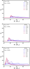 |
Fig. A.1. Mass–radius exponent as function of mass for our model with an initially 50 M⊙ star for different core helium abundances. |
Appendix B: Details for our binary evolution models
In Figs. B.1 and B.2 we show the time evolution of the mass-transfer rate for all our binary evolution models (except for the conservative systems; see Fig. 12. Table B.1 gives the key parameters of all binary models we computed here. It also gives the X-ray lifetime tX, which we define as the time period during which the accretion luminosity exceeds 1033 erg s−1. To estimate this, we introduce the quantities LX,Edd defined as the Eddington-limited accretion luminosity after half of the X-ray lifetime has passed. We define the quantity LX,max in the same manner as LX,Edd, but under the condition that the accretion was not Eddington limited, that is, as if the entire transferred mass were accreted by the compact object. We instead use the luminosity values in the middle of the mass-transfer phase because the arithmetic mean over time would be distorted by the initial peaks of the mass-transfer rate that appear in some calculations. In some models these peaks are two orders of magnitude above the long-term mass-transfer rate and last for roughly a tenth of the mass-transfer phase. The arithmetic mean would hence be shifted by one order of magnitude above the long-term X-ray luminosity. Our definition avoids this distortion and gives a better estimate of the typical luminosity during the mass transfer.
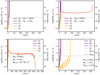 |
Fig. B.1. Evolution of the mass-transfer rate for three initial models and an NS accretor. The right axis in indicates the X-ray luminosity corresponding to the mass-transfer rate (not Eddington limited) assuming an accretion efficiency of η = 0.15. The dashed line indicates the Eddington-accretion limit of the accretor. |
Summary table of our computed binary evolution models.
All Tables
All Figures
|
Fig. 1. Mass–radius exponent of the Roche radius (Eq. (25)) as a function of mass ratio q. The different colours denote different mass-loss modes. For the blue line the entire mass is transferred and re-emitted isotropically, while for the green line the entire transferred mass is accreted. |
| In the text | |
|
Fig. 2. Mass–radius exponent (blue) of our initial 60 M⊙ model evolved to a central helium abundance of 0.8, and a H/He gradient of |
| In the text | |
|
Fig. 3. Mass–radius exponent of our initial 60 M⊙ model in the same way as for the blue line in Fig. 2, but here for models where the internal helium gradient dY/dm has been artificially adjusted (see Sect. 2) to values indicated in the legend. |
| In the text | |
|
Fig. 4. Maximum value of the mass–radius exponent ζR as a function of the chosen internal helium gradient dY/dm for stellar models derived from three different initial masses as indicated in the legends. Different colours indicate different core helium abundances at the start of the mass-loss experiments (see Sect. 2). |
| In the text | |
|
Fig. 5. Mass density as function of radius for our initially 60 M⊙ models with Ycore = 0.8 and |
| In the text | |
|
Fig. 6. Mass–radius exponent as function of stellar mass, with the three models displayed in Fig. 5 as initial models before assuming a constant mass-loss rate of 10−5 M⊙ yr−1. The colours correspond to the density profiles in Fig. 5. |
| In the text | |
|
Fig. 7. Mass–radius exponent ζR (grey), stellar radius R (blue), and radii where the gas pressure contributes only 15% (R15) and 30% (R30) to the total pressure (see text), as function of the remaining stellar mass for the three models with different values of the mixing length parameter αML shown in Fig. 6 (the lines for ζR are identical). All radii are measured in units of the initial stellar radii R0, which can be read off Fig. 5. |
| In the text | |
|
Fig. 8. Top panel: helium surface abundance as function of the total mass of the two stellar models from which the initial donor star models for our binary evolution calculations are derived. They are constructed such that mass located above the lines labelled a to e was removed before the binary calculation was started. Bottom panel: mass–radius exponent for the models as a function of the remaining stellar mass. Dashed lines correspond to the masses (labels a to e) in the upper panel. |
| In the text | |
|
Fig. 9. Evolutionary properties of our model d2ns0, neglecting a 2 M⊙ NS companion and stellar winds. Top panel: surface helium mass fraction of the donor star as function of time during the mass-transfer phase. Bottom panel: evolution of the mass-transfer rate for the same model (left Y-axis). The right axis indicates the X-ray luminosity corresponding to the mass-transfer rate (not Eddington limited) assuming an accretion efficiency of η = 0.15. The dashed line gives the Eddington accretion limit for the NS that is applied in this calculation. Despite the high initial mass ratio of 16.8, the model settles into a stable mass transfer for about 0.25 Myr, with a mass-transfer rate of about the rate of the mass transfer on a nuclear timescale. |
| In the text | |
|
Fig. 10. Hertzsprung–Russel diagram for the donor star of binary model d2ns0. Black dots correspond to time differences of 104 yr. |
| In the text | |
|
Fig. 11. Evolution of the orbital period derivative Ṗ/P of our model d2ns0 shown in Fig. 9 as given by the numerical simulation (orange line), together with our analytic estimate for the same model (see text; yellow line). Overplotted are the empirical decay rates of ten SGXBs as inferred by Falanga et al. (2015), who give six measured values with 1σ error bars (blue dots; for most of these, the error bar is smaller than the size of the dot) and four upper limits (blue arrows). We note that the time axis has no meaning for the period derivatives of the observed sources. |
| In the text | |
|
Fig. 12. Evolution of the mass-transfer rate for the same model as shown in Fig. 9 (left Y-axis) (Model d2ns0), but here calculated assuming conservative mass transfer. |
| In the text | |
|
Fig. 13. Evolution of the mass-transfer rate as function of time for our model b1bh0, which starts with a 42.5 M⊙ supergiant and a 10 M⊙ BH in an 18 d orbit. |
| In the text | |
|
Fig. 14. Spectroscopic Hertzsprung–Russel diagram including data for SGXBs from Conti (1978; green crosses) and Falanga et al. (2015; blue crosses). The name of the source is added to the symbols. The parentheses include the donor masses as measured by Conti (1978) and Falanga et al. (2015). The grey dashed lines are tracks from single-star evolutionary models (Brott et al. 2011). The grey numbers indicate the initial mass of the corresponding stellar model. Red and orange lines indicate the evolution of our binary models. The starting point of each model is labelled with a blue star. The black dots correspond to time steps of 50 000 years. |
| In the text | |
|
Fig. 15. Donor radius as a function of mass in thermal equilibrium (blue). The red lines show the Roche radius as a function of donor mass during the binary calculation that includes a 10 M⊙ accretor and no stellar wind of the donor. The yellow lines show the Roche radius after the binary calculation has stopped and CE is initiated. The orbital separation and hence the Roche radius was inferred using the energy budget description of CE. The green area marks the position of the H/He transition layer. |
| In the text | |
|
Fig. 16. Evolutionary tracks for solar and SMC metallicity during core hydrogen burning (Brott et al. 2011). |
| In the text | |
|
Fig. A.1. Mass–radius exponent as function of mass for our model with an initially 50 M⊙ star for different core helium abundances. |
| In the text | |
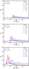 |
Fig. A.2. As Fig. A.1, but for our 60 M⊙ star model. |
| In the text | |
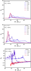 |
Fig. A.3. As Fig. A.1, but for our 80 M⊙ star model. |
| In the text | |
|
Fig. B.1. Evolution of the mass-transfer rate for three initial models and an NS accretor. The right axis in indicates the X-ray luminosity corresponding to the mass-transfer rate (not Eddington limited) assuming an accretion efficiency of η = 0.15. The dashed line indicates the Eddington-accretion limit of the accretor. |
| In the text | |
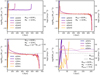 |
Fig. B.2. Similar to Fig. B.1, but with a BH accretor, η = 0.06. |
| In the text | |
Current usage metrics show cumulative count of Article Views (full-text article views including HTML views, PDF and ePub downloads, according to the available data) and Abstracts Views on Vision4Press platform.
Data correspond to usage on the plateform after 2015. The current usage metrics is available 48-96 hours after online publication and is updated daily on week days.
Initial download of the metrics may take a while.