| Issue |
A&A
Volume 681, January 2024
|
|
|---|---|---|
| Article Number | A31 | |
| Number of page(s) | 18 | |
| Section | Stellar structure and evolution | |
| DOI | https://doi.org/10.1051/0004-6361/202347090 | |
| Published online | 04 January 2024 | |
Forming merging double compact objects with stable mass transfer
1
Institute of Astronomy, KU Leuven, Celestijnlaan 200D, 3001 Leuven, Belgium
e-mail: This email address is being protected from spambots. You need JavaScript enabled to view it.
2
Dept. Astrophysics/IMAPP, Radboud University Nijmegen, Nijmegen, NL, The Netherlands
Received:
1
June
2023
Accepted:
9
September
2023
Abstract
Context. Merging double compact objects (COs) are one of the possible endpoints of the evolution of stellar binary systems. As they represent the inferred sources of every detected gravitational wave (GW) signal, modeling their progenitors is of paramount importance both to gain a better understanding of gravitational physics and to constrain stellar evolution theory.
Aims. Stable mass transfer (MT) between a donor star and a black hole (BH) is one of the proposed tightening mechanisms to form binary BHs that merge within the lifetime of the universe. We aim to assess the potential of stable non-conservative MT to produce different pairings of compact objects including BHs, neutron stars (NSs) and white dwarfs (WDs).
Methods. We investigated the conditions (orbital periods and mass ratios) required for MT between a star and a CO to be stable and to lead to binary COs that merge within a Hubble time. We use published results on the response of the stellar radii to rapid mass loss, covering different evolutionary stages and masses. Coupled with analytical models of orbital evolution, we determined the boundary for unstable MT as well as the post-interaction properties of binaries undergoing stable MT. In addition, we investigated the impact of the angular momentum loss prescription in the resulting hardening by accounting for both the isotropic re-emission from the accretor’s vicinity and mass outflow from the second Lagrangian point.
Results. Stable MT in systems with a CO + Roche lobe-filling star, in the completely non-conservative limit of isotropic re-emission from the vicinity of the accretor, is shown to be able to form any pair of merging double COs, with the exception of WD + BH and with a limited parameter space for NS + NS. Considering the possibility of mass outflow from the Lagrangian point L2, the resulting parameter space for GW progenitors is shifted toward smaller initial mass ratios (defined as the ratio of the donor mass over the CO mass), consequently ruling out the formation of NS + NS pairs while allowing the production of merging WD + BH binaries. We compare our results with observations of single-degenerate binaries and find that the conditions for the stable MT channel to operate are present in nature. We then show that stable MT in the isotropic re-emission channel can produce merging binary BHs with mass ratios > 0.1, consistent with the majority of inferred sources of the third gravitational wave transient catalogue. Enhanced angular momentum loss from L2 increases the minimum final mass ratio achievable by stable MT.
Key words: gravitational waves / X-rays: binaries / stars: evolution / binaries: general
© The Authors 2024
 Open Access article, published by EDP Sciences, under the terms of the Creative Commons Attribution License (https://creativecommons.org/licenses/by/4.0), which permits unrestricted use, distribution, and reproduction in any medium, provided the original work is properly cited.
This article is published in open access under the Subscribe to Open model. This email address is being protected from spambots. You need JavaScript enabled to view it. to support open access publication.
1. Introduction
Ground-based gravitational wave (GW) observatories of the LIGO, Virgo, and KAGRA (LVK) network have successfully identified coalescing compact objects (COs) originating from binary black holes (BHs), binary neutron stars (NSs), and binaries containing both a BH and a NS. Signals from these sources are compiled in the third gravitational-wave transient catalogue (GWTC-3, Abbott et al. 2023) and currently form a sample of over 90 detections, expected to grow significantly with future observing runs. In the next decade, third-generation detectors such as the Einstein Telescope (Maggiore et al. 2020) will provide hundreds of thousands of detections per year (Hall & Evans 2019), and the Laser Interferometer Space Antenna (Amaro-Seoane et al. 2017) will open up the frequency range of merging binary white dwarfs (WDs).
While the observed GW sample is increasing and progressively revealing new types of sources, our theoretical understanding of the evolutionary channels that form them is still limited. The main formation pathway leading to BH + BH and BH + NS mergers is still a matter of debate. On the one hand, dynamical interactions in globular clusters (Kulkarni et al. 1993; Sigurdsson & Hernquist 1993; Portegies Zwart & McMillan 2000), young stellar clusters (e.g., Mapelli 2016) or in isolated hierarchical systems (e.g., Thompson 2011) are predicted to contribute in forming close double BHs. On the other hand, isolated binary evolution scenarios rely either on a process that could prevent stars in very close binaries from expanding, like chemically homogeneous evolution (Marchant et al. 2016; Mandel & De Mink 2016), or on a hardening mechanism that allows wide binaries to come close enough.
Two main hardening mechanisms have been proposed for isolated binaries: evolution of the binary through a common envelope (CE) phase (Paczynski et al. 1976) or a stable mass transfer (MT) episode via Roche lobe overflow (van den Heuvel et al. 2017). The CE scenario was first contemplated in the context of the evolution of single-degenerate binaries with WD objects (e.g., Sparks & Stecher 1974; Chau et al. 1974), then introduced to explain the origin of cataclysmic variable stars (Webbink 1975), and subsequently suggested as the origin of Type I supernovae (SNe, Webbink 1984). CE was also advanced as the standard, late-evolutionary channel toward double degenerate binaries, both in the context of the final evolution of massive X-ray binaries as well as in the formation of NS binaries (van den Heuvel et al. 1976) and double WDs (e.g., Iben 1984). During such CE phase, the components of the binary system are engulfed by a common gaseous envelope; the resulting drag dissipates energy (and momentum) and dramatically shrinks the orbit. This process is expected to happen on a dynamical timescale, and the survival of the shrinked binary is subject to the envelope structure and companion masses.
Conversely, stable MT via Roche lobe overflow implies a quiet, long-lived phase of tightening (or broadening) of the system’s orbit. This happens on the thermal or nuclear timescale of the donor star and depends on the evolutionary stage of the donor itself. During a stable MT episode, the donor keeps its radius close to that of its Roche lobe, while material from its envelope escapes the star’s gravitational well and is transferred to the companion. The MT rate is governed by the response of the donor’s own radius to mass loss, and by the Roche lobe radius response. The mechanism is self-regulating (i.e., a maximum MT rate is expected to be reached and, subsequently, quenched), and thus dubbed stable.
While stable MT is usually involved in interacting non-degenerate binary systems before the formation of the first CO (e.g., Dominik et al. 2012; Langer et al. 2020), CE evolution has been considered the classical hardening channel toward the merging double-degenerate configuration, after the first CO is already formed (e.g., Belczynski et al. 2016; Liu et al. 2022). However, van den Heuvel et al. (2017) recently argued that the role of stable MT might be crucial in tightening the orbit of systems composed by a donor and a CO. This evolutionary scenario hypothesizes the MT episode to be completely non-conservative, and the avoidance of a CE episode to be dependent on the mass ratio of the system.
More specifically, the assumption of complete non-conservativeness has been translated in the past into modeling mass leakage from the system in the vicinity of the first-born CO with its specific angular momentum, in the isotropic re-emission channel (see van den Heuvel et al. 2017), usually justified by super-Eddington accretion rates in proximity to a compact accretor. However, the isotropic re-emission channel is just one possibility. At very high MT rates, systems can potentially experience outflows of mass through the L2 Lagrangian point (Lu et al. 2023), which would lead to further orbital shrinkage. The presence of a circumbinary outflow from systems such as the galactic microquasar SS433 could support this possibility (Fabrika 1993).
Population synthesis techniques are key to understanding the increasing sample of merging double COs via any kind of evolutionary channel, and recent studies have shown that the contribution from stable, non-conservative MT to the observed sample of merging binary BHs can be substantial and even larger than that from the CE channel (Neijssel et al. 2019; Bavera et al. 2021). There are however uncertainties in the critical mass ratios for CE. As the response of a star to mass loss depends on the structure of its envelope, several classical (e.g., Paczyński 1965) and more modern (e.g., Pavlovskii & Ivanova 2015) studies made use of stellar structure models to survey ranges of mass ratios and orbital periods for (un)stable MT; their results are subsequently implemented in binary population synthesis codes as physically motivated criteria for identifying CE. In particular, population synthesis studies usually assume a direct correlation between a specific stellar evolutionary stage with the (un-)successful CE survival (see, e.g., the mass ratio thresholds from Hjellming & Webbink 1987 and Hurley et al. 2002). This approach gives an overestimate of the CE channel contribution to binary BHs (Marchant et al. 2021). Furthermore, the adopted critical mass ratios for CE evolution may lead to an oversimplification of the progenitors’ initial conditions to produce merging double COs (Gallegos-Garcia et al. 2021).
The aim of this work is to assess the potential of non-conservative stable MT as a candidate evolutionary channel toward the merging double CO configuration. We put the emphasis on the production of all the different pairings of compact objects other than just the double BH scenario. We did so by investigating the parameter space of progenitor systems composed by a CO orbiting a Roche lobe-filling donor, using existing results on the response to a star to rapid MT (Ge et al. 2010, 2015, 2020) to resolve the boundary of critical mass ratios for CE evolution. We then computed the orbital shrinkage of the systems with angular momentum balance arguments and finally studied the possibility of the formation of the different GW source pairings. Crucially, our approach is semi-analytical, as it does not rely on the tools of population synthesis and/or detailed binary interaction simulations. Section 2 provides the methodology; we present our results for selected donor star’s masses in Sect. 3, while Sect. 4 compares the results with observations. We conclude by summarizing the main findings and discussing remarks and prospective work in Sect. 5.
2. Methodology
We always refer to quantities concerning the donor (accretor) in the MT episode with the subscript d (a), and to quantities at the start (end) of the MT episode with i (f). If neither i nor f is specified, we refer to quantities as variables in the evolution of the systems. We define the binary mass ratio, q, between a donor of mass md and an accretor of mass ma, at an arbitrary stage, as
 (1)
(1)
We also define a stripping factor, αcore, as the fraction of initial donor’s mass, md, i, that remains after the MT episode, leaving the donor with mass md, f:
 (2)
(2)
Therefore, the final mass ratio of the system is
 (3)
(3)
Sections 2.1 and 2.2 set the hypothesis on the shrinking mechanism and the merging time calculation and also present a functional study for a simple case of fixed donor mass md, i = 32 M⊙. Section 2.3 discusses the instability boundary calculation, with a description of the properties used from existing simulations in Sect. 2.4. Section 2.5 sets the constraint on the final donor star’s radius. Section 2.6 shows how we model mass outflow from L2.
2.1. The parameter space for GW progenitors
We hypothesize a completely non-conservative MT episode: the first-born CO is assumed to be accreting material from the donor at a super-Eddington rate, thus expelling mass from its surroundings with the accretor’s specific angular momentum. This scenario has been referred to as isotropic re-emission.
We defined the efficiency, ϵ, of the MT (i.e., the fraction of accreted mass, Δma, when the donor transfers Δmd), as
 (4)
(4)
Here, β = 0 is the limit of conservativeness (everything is accreted) and β = 1 describes the isotropic re-emission assumption. Assuming that β is a constant of evolution, an exact orbital solution for the period shrinkage, Pi/Pf, can be found by angular momentum balance arguments (Soberman et al. 1997):
 (5)
(5)
where, within our assumption of β = 1, the accretor mass will satisfy ma, i = ma, f, so that the final and initial mass ratio of the system are related by qf = αcore qi.
To assess if the binary system at the end of the MT can evolve into a GW source, we adopted the analytical expression for the delay time tmerge of an inspiraling binary (Peters 1964),
 (6)
(6)
 (7)
(7)
which holds for a circular orbit with final orbital separation af and neglects other sources of radiation apart from the gravitational quadrupole one. We therefore implicitly assume that the second born CO, at the start of the inspiral phase, has the post-MT mass md, f and starts the inspiraling at the post-MT separation af. We relax this assumption in Sect. 3.2.
2.2. Constant αcore
The initial conditions required for a GW progenitor system can be constrained by looking at the initial accretor mass vs initial orbital period (ma, i − log Pi) parameter space. To do so, we combined Eq. (5) with Eq. (6) and Kepler’s third law for the final orbital separation, af. By imposing the merging time being less than a Hubble time tH, in other words tmerge < tH ≃ 13.8 Gyr, one finds
 (8)
(8)
This condition can be generalized to other hardening channels if the value of Pi/Pf is a function of the initial and final mass ratios. We used this later when we considered outflows from the L2 point.
A visualization of the locus for fixed values of the stripping factor, αcore, and a donor initial mass of md, i = 30 M⊙ is shown in Fig. 1. The parameter space that stands below the solid curves is the promising portion for the initial properties of progenitor systems of GW sources. Systems with a larger initial orbital period, Pi, are more likely to originate sufficient shrinkage for a GW merger at large initial mass ratios, qi ≫ 1. These systems are also farther from reaching the mass ratio inversion (around q = 1, the colored diamonds along the curves) during the MT episode, and thus less likely to switch from orbital contraction to orbital expansion due to MT. The effect of different stripping factors, αcore, labeled along the correspondent curves, is also shown: we see that more stripping (moving from the αcore = 0.5 to the αcore = 0.3 curve) implies a less favorable parameter space for GW mergers after the mass inversion q = 1, as the broadening of the orbit during the MT is favored. On the other hand, less stripping of the donor (moving from the αcore = 0.5 to the αcore = 0.8 curve) allows for less extreme qi to form GW mergers.
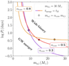 |
Fig. 1. Locus (see Eq. (8)) for the formation of a GW source through stable MT with a 30 M⊙ donor as a function of the CO accretor mass, ma, i, and orbital period, Pi. The solid curves represent the upper bounds on initial periods log Pi, to achieve a delay time of tmerge = tH; different stripping factors, αcore, are labeled along the corresponding curves. Colored diamonds correspond to the point, along their respective curves, at which the MT episode is expected to invert the mass ratio. |
2.3. The common envelope boundary
The assumption of a constant stripping factor is useful for illustrative purposes, but we want to trace a more accurate boundary in the parameter space (ma, i − Pi) of GW progenitors. To this purpose, we also want to take into account that, keeping a fixed donor mass, md, i, for more extreme initial mass ratios we expect to encounter the boundary of critical mass ratios, qcrit, for CE evolution (Soberman et al. 1997).
The (in-)stability of a MT episode is usually characterized with mass-radius exponents. We followed Soberman et al. (1997) in writing the donor’s mass-radius critical (or adiabatic) exponent ζad:
 (9)
(9)
From the calculations of Ge et al. (2020) we took ζad(R, M), that is the adiabatic mass radius exponent as a function of the stellar radius (encoding its evolutionary stage) and mass (see more in Sect. 2.4). The orbit response to the MT episode is quantified by the donor’s Roche lobe mass-radius exponent, ζRL:
 (10)
(10)
Performing the stability analysis for the adiabatic MT episode amounts to comparing the two dimensionless exponents ζRL and ζad. Stability requires that, after a mass loss-induced perturbation, δmd < 0, the star’s radius remains contained within its Roche lobe; in other words, ζad > ζRL. If this is not satisfied, the MT is unstable and we expect CE evolution to happen.
The donor’s Roche lobe mass-radius exponent, ζRL, must be computed according to the evolution of the binary system, so an assumption of the MT mode is needed; indeed, analytical expressions are provided in Soberman et al. (1997). In the case of conservative MT, one derives
 (11)
(11)
where we adopted the Eggleton (1983) prescription for RRL:
 (12)
(12)
with a being the orbital separation.
If we include non-conservativeness, ϵ < 1, by switching on an efficiency β > 0 for isotropic re-emission as in Eq. (4), the Roche lobe mass-radius exponent,  , assumes the following general form:
 (13)
(13)
In the assumption of fully non-conservative MT, i.e. ϵ = 0, and purely isotropic re-emission, i.e. β = 1, the above expression translates into
 (14)
(14)
where the superscript “iso” stands for isotropic re-emission.
By comparing the adiabatic mass-radius exponent of donor stars, ζad(Rd, i, md, i), with a family of Roche lobe mass-radius exponents,  , sharing the same initial mass, md, i, and radius, Rd, i, the threshold in mass ratio for which MT is unstable,
  , is found by requesting
 (15)
(15)
where we called  the critical mass ratio of an interacting binary system at the start of the unstable MT episode.
Once we derived critical mass ratios, we could build a common envelope boundary in the (ma, i − Pi) parameter space, for fixed md, i, with the following reasoning. Let us consider a donor star of radius Rd, i, which we assume to be equal to the Roche lobe radius, RRL, i, at the onset of MT. The value of ζad of the star at the evolutionary stage in which it fills its Roche lobe then yields the critical mass ratio  for unstable MT, by solving Eq. (15). Combining the information of
  and Rd, i = RRL, i, we can then infer a critical period for the instability boundary using Kepler’s third law:
![Mathematical equation: $$ \begin{aligned} P_{\mathrm{i, crit} }=\dfrac{2\pi }{\left[G(m_{\mathrm{d,i} }+m_{\mathrm{a,i} })\right]^{1/2}}\left.\left(\dfrac{R_{\rm RL}}{a}\right)\right|_{q^{\mathrm{iso} }_{\mathrm{crit} }}^{-3/2}R_{\mathrm{d,i} }^{3/2}. \end{aligned} $$](/articles/aa/full_html/2024/01/aa47090-23/aa47090-23-eq22.gif) (16)
(16)
Here we isolated the factor RRL/a, which is immediately known at the wanted mass ratio,  (see Eq. (12)). Notice that this factor was evaluated at
  , in other words at the start of the MT episode. We determined ζad as a function of the donor stars’ initial mass, md, i, and radius, Rd, i, and we used the simulations of Ge et al. (2020), described in more detail in Sect. 2.4.
2.4. Ge et al. simulations
The set of simulations from Ge et al. (2020) covers a grid of Population I stars, Z = 0.02, spanning the zero age main sequence (ZAMS) mass range 0.10 ≤ md, i/M⊙ ≤ 100 and evolutionary stages from ZAMS through the terminal age main sequence (TAMS), to the helium ignition, red giant branch (RGB) and asymptotic giant branch (AGB), as the case may be. Following the methodology described in Ge et al. (2010), they build “adiabatic mass loss sequences”: starting from an initial stellar model at an arbitrary state in its evolution, mass is removed from the surface while the stellar interior relaxes adiabatically to a new state of hydrostatic equilibrium. These adiabatic mass loss sequences yield ζad, fixing the critical mass ratio for dynamical timescale MT. The Hertzsprung-Russell diagram of the mass loss sequences, for 1.6 ≤ md, i/M⊙ ≤ 100, is shown in Fig. 2.
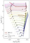 |
Fig. 2. Hertzsprung-Russell diagram of the adiabatic mass loss sequences from Ge et al. (2020), labeled by their mass. Different evolutionary phases (TAMS, helium ignition and end of core He-burning) are highlighted with different icons (unfilled triangle, circle, and square). The empirical Humphrey-Davidson (HD) limit, in dashed red (Humphreys & Davidson 1979), is also reported. |
We used the critical mass-radius exponents, ζad, from Ge et al. (2020) to derive the threshold for unstable MT using Eq. (15). Their mass-radius relations’ slopes are derived in the fully conservative approximation, namely by assuming a Roche lobe response, as in Eq. (11). They nevertheless claim that their exponents can also be used in the non-conservative cases to find critical mass-ratios for CE (see Ge et al. 2010).
From their simulations we also took the core mass, defined as the mass coordinate at which the helium abundance is halfway between the surface helium abundance and the maximum helium abundance in the stellar interior. We assumed this mc to be the remaining mass after the MT episode, so that our stripping factor αcore became
 (17)
(17)
Thus, if the binary system survives the MT episode, we assume it to be composed by an accretor with mass ma, f and a donor with md, f = mc. There is a subtlety though: during the main sequence (MS), mc as defined by Ge et al. (2020) recedes over a nuclear timescale. This receding resembles the monotonous one, predicted by single star evolution, of the convective core of massive stars. Adopting such mc before TAMS can thus lead to a consistent overestimation of the core left after the MT episode, as a Case A MT is expected to quickly strip the donor and make the core retract deeper. In this respect, we modeled the remaining mass as follows:
namely, we used the core mass at TAMS, mc|TAMS, as the remaining mass, md, f, after MT episodes initiated by pre-TAMS donors. This is still expected to be an overestimate of the final mass after MT.
For the largest initial donor star masses, namely 50 ≤ md, i/M⊙ ≤ 100, we limited our analysis to those initial models in the mass loss sequences that fall under the empirical Humphrey-Davidson limit (dashed red line in Fig. 2).
Figure 3 shows how the critical mass ratios for unstable MT are determined using two fixed donor masses from the Ge et al. (2020) grid. At any evolutionary stage, the critical mass ratios for isotropic re-emission,  , are shifted, with respect to the conservative case, toward smaller values (i.e., to larger accretor masses ma, i). Massive stars experience significant radial expansion in the Hertzsprung gap before developing a convective envelope, while lower mass stars develop a convective envelope and start rising on the Hayashi line without significant expansion after the MS. In terms of ζad, this results in the more massive star experiencing a monotonic increase of ζad over a large range of radii, while the opposite is the case for lower mass stars.
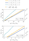 |
Fig. 3. Functional dependence of ζRL on the binary mass ratio qi ≡ md, i/ma, i, compared to the adiabatic index, ζad, for donor stars of 32 M⊙ (top panel) and 2 M⊙ (bottom panel) of different radii. The different colors of the solid lines show the conservative limit, ϵ = 1 (golden), and the completely non-conservative cases of purely isotropic re-emission, β = 1 (dark blue), and mass outflow from L2 (light blue), see the discussion in Sect. 2.6. Critical mass ratios, ζad, for the MT to be unstable, as calculated by Ge et al. (2020), are shown as horizontal lines (labeled by the donor star radius). For each radius and mode of MT, the critical mass ratio corresponds to the crossing points between ζad and ζRL. |
2.5. Final orbital separations
We computed the final orbital separations, af, by using the orbital shrinkage equation, Eq. (5), and Kepler’s third law. Even if the instability criterion is satisfied, we find cases where the predicted orbital separations af at the end of the MT episode are too small to contain a stripped helium star of the expected final mass. This is indicative of the occurrence of delayed dynamical instability (Hjellming & Webbink 1987) where, even if the start of the MT phase is stable, it can become unstable before the donor is fully stripped.
We thus set a hard boundary for the final Roche-lobe radius, RRL, f, of the donor at the end of the MT episode. We computed a set of MESAPaxton et al. (2010), 2013, 2015, 2018, 2019) models of helium zero age main sequence (He-ZAMS) stars with initial masses 0.275 M⊙ ≤ md, f ≤ 52.75 M⊙. We expanded the solar metallicity set of He-ZAMS in Poniatowski et al. (2021) with MESA v15140, and produced a set of values for the radius at the He-ZAMS stage, RHe − ZAMS, for each model. We then assumed that the limiting orbital separation for our model to hold is the one at which the final donor’s Roche-lobe radius ,RRL, f, is equal to the He-ZAMS radius, RHe − ZAMS, of the He-ZAMS model with corresponding stripped star mass. Namely, we imposed:
 (18)
(18)
Physically, the condition in Eq. (18) also implies an equilibrium configuration of our final stage after the MT episode. However, it might be an oversimplification. Investigating the details of this hard boundary requires detailed MESA modeling of the binary interactions and is planned in a follow-up of this work.
2.6. Modeling L2 outflow
2.6.1. Shrinkage of the orbit with L2 outflow
Isotropic re-emission is a simplified model of the dynamics of ejected material in a binary, and real binary systems could exhibit more complex outflows. For WD accretors, high MT rates ( ) are expected to result in rapid expansion and the formation of a red giant star (Nomoto 1982; Cassisi & Iben 1998; Shen & Bildsten 2007; Wolf et al. 2013). In a binary system this expansion would lead to overflow of the outer Lagrangian points. It has also been argued that, at high MT rates onto NS or BH companions, the accretion disk would grow and start ejecting most of the mass transferred through L2 (Lu et al. 2023), preventing in some cases the expansion of the orbit after the mass-ratio inversion. Such additional shrinkage sourced by L2 angular momentum loss can therefore be key to favoring the formation of merging double COs, but also impact the stability of MT.
In this respect, we modeled the L2 outflow in the form of a modified rule for the period shrinkage, Pi/Pf, using a generalized efficiency, ϵ, of the MT:
 (19)
(19)
Here, β + υ = 0 is the limit of conservativeness and υ = 1 corresponds to the assumption of all mass being lost through L2. The υ efficiency is still modeled as a constant during the MT episode.
We first numerically computed the distance between the second Lagrangian point, xL2, and the center of mass, xcm ≡ 1/(1 + q), of the system; we called such distance xL2 − xcm, expressed in units of orbital separation, a. We considered a Cartesian system with an origin (x = 0, y = 0, z = 0) located at the center of the donor star, with a  axis pointing toward the accretor and
  toward the direction of the angular momentum vector. We then constructed the following fit to the numerical solution for (xL2 − xcm)2:
![Mathematical equation: $$ \begin{aligned} \left(x_{L_2}-x_{\mathrm{cm} }\right)^2(q)\simeq 1+\sum _{n=1}^{5} a_n\times \left\{ \begin{matrix} q^{-(n-n_0)}& q\ge 1\\ [3pt] q^{(n-n_0)}& q{< }1\\ \end{matrix} \right. \end{aligned} $$](/articles/aa/full_html/2024/01/aa47090-23/aa47090-23-eq33.gif) (20)
(20)


The fit has a fractional error < 0.1% over the range 1 ≤ q < +∞. Thanks to the symmetry of the problem, the L2 position (xL2 − xcm)(q) for q < 1 is obtained from −(xL2 − xcm)(1/q).
Material ejected through L2 is assumed to carry away a specific angular momentum, j, corresponding to this Lagrangian point, j = a2(xL2 − xcm)2Ωorb, with Ωorb being the Keplerian angular frequency of the orbit. Following Soberman et al. (1997), the evolution of the orbital period, Pi/Pf, as a function of the mass ratio and including both isotropic re-emission and L2 mass loss can then be computed analytically as
![Mathematical equation: $$ \begin{aligned}&\dfrac{P_{\mathrm{i} }}{P_{\mathrm{f} }}=\exp \left[-3\beta \left(q_{\mathrm{f} }-q_{\mathrm{i} }\right)\right]\left(\dfrac{1+q_{\mathrm{f} }}{1+q_{\mathrm{i} }}\right)^{3\beta -1}\left(\dfrac{q_{\mathrm{f} }}{q_{\mathrm{i} }}\right)^3\times \nonumber \\&\qquad \quad \exp \left[-3\upsilon \int _{q_{\mathrm{i} }}^{q_{\mathrm{f} }} f(q)\,\mathrm{d}q\right],\text{with } \end{aligned} $$](/articles/aa/full_html/2024/01/aa47090-23/aa47090-23-eq36.gif) (21)
(21)
![Mathematical equation: $$ \begin{aligned}&f(q)\equiv \dfrac{(1+q)}{q}\,\left[x_{L_2}-x_{\mathrm{cm} }\right]^2. \end{aligned} $$](/articles/aa/full_html/2024/01/aa47090-23/aa47090-23-eq37.gif) (22)
(22)
Using the fit for (xL2 − xcm)2 in Eq. (20), the integral ∫qf(q) dq can be computed analytically, and we refer to Appendix A for more details about its solution.
With such a modified period shrinkage rule, one can immediately define the parameter space (ma, i, log Pi) for GW progenitor systems by using Eq. (8) with the adapted Pi/Pf of Eq. (21) and switching on an efficiency for L2 mass loss with υ > 0. Keeping the completely non-conservative limit ϵ = 0, we then had β = 1 − υ. The locus for fixed values of the stripping factor, αcore, and a donor initial mass of md, i = 30 M⊙ is shown in Fig. 4, with analogous notation as Fig. 1. As expected, we see that the extra source of angular momentum loss implies that the locus for the formation of a gravitational wave source moves toward more massive accretors. However, the expected change in orbital evolution also impacts the stability of MT, as we discuss in Sect. 2.6.2.
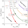 |
Fig. 4. Same diagram as in Fig. 1 with the modified shrinkage relation Pi/P in Eq. (21), a fixed stripping factor, αcore = 0.5, and a variable efficiency for L2 mass outflow, υ. Different efficiencies, υ, are labeled along the correspondent curve. |
2.6.2. Common envelope boundary with L2 outflow
As an outflow from L2 during the MT episode has consequences on the orbit evolution, the orbit response to MT is also affected and thus  in Eq. (13) needs to be properly modified:
 (23)
(23)
and f(q) is defined by Eq. (22). Since υ > 0 positively shifts the value of  , the expected effect on the critical mass ratios,
  , is a shift toward lower values (or accordingly, more massive CO accretors) with respect to
  . This is clearly shown in Fig. 3 for the limiting case of υ = 1. Analogously to what we did in Sect. 2.3 for
  , we determined
  for a donor with a given initial mass, md.i, and radius, Rd, i, in the presence of υ > 0 and ϵ = 0 by imposing the condition:
 (24)
(24)
3. Results
This section presents the results of the favorable parameter space for GW progenitor systems, in the form of (ma, i, log Pi) diagrams with a fixed donor mass, md, i. We show the results for a BH direct collapse (Sect. 3.1), NS remnant with kick velocity (Sect. 3.2), and WD accretors (Sect. 3.3); just one example for fixed md, i is shown for each case. The full set of results for 2 < md, i/M⊙ < 100 will be made publicly available at the time of publication on Zenodo1.
3.1. BH progenitor as the donor
When the initial mass, md, i, of the donor is md, i ≥ 25 M⊙, we assume that, after a later evolution of the stripped star following the MT episode, the star undergoes direct collapse into a BH. As such, we modeled the evolutionary history from the end of the MT episode until merging as if the direct collapse happens immediately after the MT. Therefore, this model ignores possible mass loss between the end of the MT phase and BH formation, which is expected to widen the orbit (see discussion in Sect. 3.4). We briefly discuss the possibility of having BHs kick for 25 ≲ md, i (M⊙)≲40 in Sec. 3.2. Afterward, the double CO system evolves only under the effect of gravitational interaction via quadrupole radiation emission (see Eq. (6)).
Figure 5 shows the parameter space (ma, i, log Pi) for GW progenitor systems that results from the described approach. The Roche lobe-filling star is a md, i = 32 M⊙ donor. Let us first consider the purely isotropic re-emission channel (solid lines). For any orbital period there is a range in mass ratio where MT is expected to be stable and to lead to sufficient hardening to produce a CO coalescence within a Hubble time. Such a strip extends between the common envelope boundary (solid red line) and the delay time boundary (solid blue line). Requiring that RRL, f > Rd, f at the end of the MT episode, as discussed in Sect. 2.5, significantly limits such a strip for more evolved donors. Nevertheless, the accretor masses, ma, f, spanned by the strip at different stages are such that 5 ≲ ma, i/M⊙ ≲ 37. Therefore, we confirm that the production of merging double BH from stable MT via isotropic re-emission is possible. This, however, relies on the assumption that such initial conditions are realized in nature, which can be informed by observations of single-degenerate binaries (see Sect. 4.1). We also rely on the assumption that the response to MT of the donor star, which potentially accreted mass from the BH progenitor in a previous evolutionary phase, is well approximated with the single star models of Ge et al. (2020).
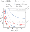 |
Fig. 5. Boundaries for unstable MT (red) and the formation of GW sources (blue) for a 32 M⊙ donor orbiting a CO of mass ma, i. The area below the gray line excludes systems for which the final orbital separation implies Rd, f < RRL, f. Results are shown for full isotropic re-emission (solid) and assuming all matter is ejected from L2 (dashed line). Different stages of evolution are illustrated by contours of constant Roche lobe radius (dotted gray line). Empty circles mark the formation of a convective envelope containing 10% of the donor’s mass. |
In Fig. 5 we also show the results after switching on an efficiency υ = 1 for L2 mass outflow. As illustrated in the simple model with fixed αcore of Fig. 4, the locus for the formation of a merging double CO is shifted toward higher accretor masses. However, the additional angular momentum loss also shifts the boundary for stability toward higher accretor masses. Nevertheless, a range in mass ratio and initial periods for merging double COs, from stable MT for υ > 0, is still predicted. The masses of the CO accretor in this strip are such that ma, i(M⊙)≳11, and thus the expected outcome is indeed merging binary BHs, though with different mass ratios with respect to the purely isotropic re-emission case.
The predicted strip for md, i = 32 M⊙ can be compared to the one derived, with a set of MESA simulations, by Marchant et al. (2021) for a 30 M⊙ metal-poor (Z = 0.00142), Roche lobe-filling donor star orbiting a CO. The results from our semi-analytical model are qualitatively consistent with the ones from their set of detailed simulations, for both the instability boundary and the merging time constraint, although our predictions overestimate the set of initial conditions that lead to a GW source (see Appendix B and Fig. B.1 for a discussion). As discussed in Appendix B, this holds for our results in the purely isotropic re-emission channel, as in their simulations the accretion rate for the stable MT episodes easily approaches the Eddington one, so that β ≃ 1 even though in the simulations the degree of non-conservativeness is not a free parameter.
Figure 6 summarizes our results for the GW merger strip in the form of a (ma, i, log Pi) diagram similar to Fig. 5, with different donor masses in the range of BH progenitors, i.e. md, i = 40 M⊙, 32 M⊙, 25 M⊙. In these diagrams we discretely vary the efficiencies for isotropic re-emission and mass outflow from L2, keeping the total ϵ = 1 − β − υ = 0. Firstly, we can see a shift toward larger accretor masses (i.e., smaller final mass ratios qf) as we increase md, i. Secondly, we notice the possibility of the second-born CO to result in either the more massive object of the merging CO + CO pair (this happens at longer initial periods) or the less massive one (lower initial periods). Thirdly, we observe that the coupling of the second-born BH with a first-born NS accretor, within the stable MT channel, is excluded.
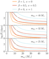 |
Fig. 6. Locus for the formation of a GW source through stable MT with 40 M⊙, 32 M⊙, 25 M⊙ donors, i.e. BH progenitors, as a function of the CO accretor mass., ma, i, and the orbital period, Pi. Different colors mark the favorable strips for merging double COs via purely isotropic re-emission (β = 1) and mass outflow from L2 with variable efficiencies υ > 0, keeping β + υ = 1. Solid black lines mark the range of known NS masses from binary systems (Tauris et al. 2017). |
Although we place no constraints on the first-born CO mass in our analysis, stellar evolution can prevent the formation of arbitrarily large BH masses, ma, i ≳ 30 M⊙, as considered in Fig. 6. At the Z = 0.02 metallicity of the Ge et al. (2020) simulation set, stellar winds potentially prevent the formation of such massive BHs (e.g., Spera et al. 2015). Nevertheless, we do not restrict the BH masses we study as we take the Ge et al. (2020) results to be also representative of lower metallicity environments, which is supported by our comparison to the stability boundary at low metallicity of Marchant et al. (2021) in Appendix B.
3.2. NS progenitor as the donor
The range of ZAMS masses, mZAMS, for leaving behind a SN remnant is a matter of debate: the upper ZAMS mass limit, classically posited as mZAMS ≲ 25 M⊙ by, for example, Fryer (1999), has recently been argued to be formed by “islands of explodability” (e.g., O’Connor & Ott 2011; Ugliano et al. 2012; Müller et al. 2016; Mabanta et al. 2019). On the other hand, the lower ZAMS mass limit is canonically set at mZAMS ≳ 8 M⊙ based evolution studies of single massive stars (e.g., Poelarends et al. 2008), but depends on metallicity (e.g., Langer 2012) and can be different for stars born in close binaries (Wellstein et al. 2001). In the following, we ignore the above complications and adopt the simplistic range 8 < mZAMS/M⊙ < 25. In particular, when the initial mass, md, i, of the donor is such that 8 ≤ md, i/M⊙ < 25, we assume that, after the MT episode and the later evolution of the stripped star, it explodes as a SN, leaving a compact NS remnant.
Since the population of galactic NSs is known to have a velocity dispersion much larger than that of OB-type stars, indicative of kicks during a SN explosion (see Lai et al. 2001 for a discussion), we also take this possibility into account in our calculations. As BHs have also been argued to have potential kick velocities at birth (see e.g., Atri et al. 2019), we also consider the case of a md, i = 32 M⊙ BH progenitor at the end of this section.
In the case of NSs, the post-SN orbital parameters have been derived by several authors (e.g. Sutantyo 1978; Hills 1983; Verbunt et al. 1990; Brandt & Podsiadlowski 1995; Kalogera 1996); in particular, we follow the notation and expressions given in Tauris et al. (1999; see Eqs. (6)–(8) of that work). We point out that the calculation of the post-SN properties given by Tauris et al. (1999) assumes a circular pre-SN orbit followed by an instantaneous SN explosion and subsequent kick.
With these same assumptions, and adopting a canonical mass of md, pSN = 1.4 M⊙ for the second-born CO, namely the NS remnant, we calculated the orbital separation, apSN, and the acquired eccentricity, epSN, of the system after the SN explosion; we used the subscript pSN to indicate the post-SN stage, to differentiate from the subscript f that we used above for the post-MT configuration. Also, as opposed to Tauris et al. (1999), we did not take into account the possible effects, on the orbit and on the first-born compact companion, of the passing shock wave from the SN (i.e., we set vim = 0 in Tauris et al. 1999).
To assess if the binary system at the end of the MT can evolve into a GW source, we adopted the analytical expression for the delay time tmerge found by Peters (1964):
![Mathematical equation: $$ \begin{aligned} t_{\mathrm{merge} }=\dfrac{12}{19}\dfrac{c_{\mathrm{pSN} }^4}{\mathcal{B} }\int _0^{e_{\mathrm{pSN} }}\mathrm{d}e\, \dfrac{e^{29/19}[1+(121/304)\,e^2]^{1181/2299}}{(1-e^2)^{3/2}}, \end{aligned} $$](/articles/aa/full_html/2024/01/aa47090-23/aa47090-23-eq46.gif) (25)
(25)
![Mathematical equation: $$ \begin{aligned} \text{ with}\quad c_{\mathrm{pSN} }^4\equiv a_{\mathrm{pSN} }^4\left[\dfrac{1-e_{\mathrm{pSN} }^2}{e_{\mathrm{pSN} }^{12/19}}\right]^4\left\{ \left[1+\dfrac{121}{304}e_{\mathrm{pSN} }^2\right]^{-870/2299}\right\} ^4. \end{aligned} $$](/articles/aa/full_html/2024/01/aa47090-23/aa47090-23-eq47.gif) (26)
(26)
This expression is the generalized form of Eq. (6) in the case of non-zero post-SN eccentricity.
To account for the possibility of kicks, we adopted the kick velocity distribution in Hobbs et al. (2005) for the second-born CO, that is, a 1D Maxwellian with dispersion 260 km s−1, and isotropic orientation in a frame of reference comoving with the SNe progenitor. For each initial orbital period, Pi, and compact object accretor mass, ma, i, we computed the post-MT orbital properties in the same way as we did for the BH progenitor in Sect. 3.1, obtaining a distribution of the post-SN properties, namely epSN, apSN due to the post-SN kick. Because of this, for each set of donor mass 8 ≤ md, i/M⊙ < 25, accretor mass, and initial orbital period, we had a probability, ptmerge < tH, of forming a merging double CO binary.
To illustrate the impact of a SN kick, we considered one specific binary system with an 8 M⊙ donor star and a 2 M⊙ accretor with an orbital period of 10 days. The binary undergoes a stable MT episode with isotropic re-emission, after which the donor star is stripped to md, f = 2.06 M⊙ and the orbital period is Pf = 0.48 days, and these are considered to be the pre-SN properties. We considered the occurrence of a kick to the resulting CO according to the distribution of kick properties described in the previous paragraph. There is a 52.5% probability that the binary is disrupted from the kick. For the remaining 47.5%, Fig. 7 illustrates the resulting distribution of post-SN eccentricities and periods: a fraction of them (35.5%) has conditions that allow for a merger within 13.8 Gyr, and the remaining 12% end up being too wide for GW radiation to drive to a merger within the age of the Universe.
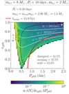 |
Fig. 7. Distribution of post-SN eccentricity, epSN, and orbital period, PpSN, for an example binary system (see Sect. 3.2 for details). Solid white lines indicate the final orbital parameters of the fixed kick velocity, w, and the variable angle, θ, formed between the kick velocity and the orbital velocity, assuming the kick to be on the orbital plane (i.e., ϕ = 0). Dashed black lines indicate the same for a fixed θ and a variable w. A thick solid red line shows the boundary separating wide (right of the curve) from merging (left of the curve) systems. |
The resulting merger probabilities are shown in Fig. 8 for the case of a donor star of md, i = 8 M⊙ under the assumption of isotropic re-emission. The favorable strip for GW mergers comprises a small interval of accretor masses, and for later evolutionary stages the common envelope boundary (solid red line) takes over and overlays any possible system with tmerge < tH. For this 8 M⊙ donor, we find that the CO accretors for which we form a GW source span, at different evolutionary stages, between 1.75 ≲ ma, i(M⊙)≲3.75. As we can observe in Fig. 9 by looking at the β = 1 contours, for the case of a md, i = 16 M⊙ and a md, i = 20 M⊙ donor we find that the range of CO accretors spans 2 ≲ ma, i(M⊙)≲10 and 3 ≲ ma, i(M⊙)≲15, respectively. For a narrow range of donor masses, just above the limit at which we expect core-collapse SNe, stable MT can then produce merging binary NSs. However, for a wider range of donor masses that would result in a NS, we require a CO accretor with a mass consistent with a BH.
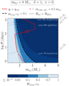 |
Fig. 8. Probability of forming a GW source through stable MT with an 8 M⊙ donor as a function of the CO accretor mass ma, i and orbital period Pi. The donor star is assumed to form a NS with an isotropic kick (see Sect. 3.2). Analogous symbols and notation, as in Fig. 5, are employed for the purely isotropic re-emission channel (β = 1). The contour color code maps the probabilities, ptmerge < tH, of obtaining merging times tmerge < tH, given the distribution of kick velocities from Hobbs et al. (2005) and isotropic kick directions, as explained in Sect. 3.2. |
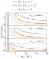 |
Fig. 9. Locus for the formation of a GW source through stable MT with 20 M⊙, 16 M⊙, 8 M⊙ donor, i.e., NS object progenitors, as a function of the CO accretor mass, ma, i, and orbital period, Pi. Contours indicate the region where the merger probability after the SN kick is ptmerge < tH > 0.1. Analogous notation to Fig. 6 is employed. |
The bottom panel of Fig. 9 shows the results for md, i = 8 M⊙ after switching on an efficiency υ = 1 for L2 mass outflow (light blue area). The pairing between NS and BH is here predicted all along the favorable GW strip. However, the additional angular momentum loss during the MT episode removes the possibility of forming a merging binary NSs, allowing solely for the formation of merging NS + BH systems where the NS is the second-born CO. The other panels in Fig. 9 show the results for md, i = 20 M⊙, 16 M⊙ and different efficiencies, β and υ. For these cases, we confirm the aforesaid prediction for merging NS + BH pairs with a second-born NS; this is true for any value of L2 outflow efficiency υ > 0.
Lastly, to investigate the effect of a possible kick imparted to a BH progenitor, we calculated the probability, ptmerge < tH, in the same fashion as for NS progenitors, for the case md, i = 32 M⊙. We assumed a) a mass loss of 10%, that is, the mass of the second-born BH was assumed to be md, pSN = 0.1 × md, f, and b) an imparted kick magnitude of 100 km s−1. The resulting parameter space for GW mergers is superimposable with the direct collapse results shown in Fig. 5. Assuming a small, fixed fraction of mass loss makes the system stay massive, and thus ptmerge < tH ≃ 1 are found below the time delay boundary at any log Pi.
3.3. WD progenitor as the donor
When the initial mass of the donor is md, i < 8 M⊙ we assume that, after the MT episode, the stripped star evolves into a WD, orbiting its compact companion with no further interaction.
Figure 10 shows the resulting diagram (ma, i, log Pi) of GW progenitors for the case of md, i = 3.2 M⊙. In the purely isotropic re-emission channel (solid lines), the favorable parameter space for merging WD + CO from stable MT is visibly limited to a thin strip of mostly systems with pre-TAMS interaction. A small post-TAMS region is also situated between the common envelope (solid red line) and the merging time (solid blue line) boundaries. The possible accretor masses, ma, i, at different initial orbital period are such that 0.75 ≲ ma, i/M⊙ ≲ 1.25: this predicts merging WD + WD pairs. As shown in Fig. 11 for the β = 1 contours, when we scale the donor mass, md, i, to larger values the strip shifts to larger values for ma, i. For md, i = 4 M⊙ in Fig. 11 (top panel), we find that the ma, i accretor masses spanned are such that 0.8 ≲ ma, i/M⊙ ≲ 1.5. We thus find space for a merging system with a first-born NS orbiting the second-born WD. On the other hand, for md, i = 2 M⊙ in Fig. 11 (bottom panel), we see that the favorable region is almost entirely suppressed.
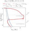 |
Fig. 10. Boundaries of unstable MT (red line) and the formation of GW sources (blue line) for a 3.2 M⊙ donor orbiting a CO of mass ma, i. Analogous symbols and notation to Fig. 5 are employed for the purely isotropic re-emission channel, β = 1. |
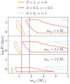 |
Fig. 11. Locus for the formation of a GW source through stable MT with 4 M⊙, 3.2 M⊙, 1.6 M⊙ donors, i.e., WD object progenitors, as a function of the CO accretor mass, ma, i, and orbital period, Pi. Analogous notation to Fig. 6 is employed. |
The middle panel of Fig. 11 shows the results for md, i = 3.2 M⊙, with an efficiency υ = 1 for L2 mass outflow (light blue area). Similar to the BH and the NS progenitor cases, the favorable strip to form a GW source via stable MT is shifted toward larger accretor masses with respect to the purely isotropic re-emission case. In this case, it could also be consistent with the formation of a WD + BH compact binary, where the WD is the second-born CO. This is also shown in the other panels of Fig. 11 with the results for md, i = 4 M⊙, 1.6 M⊙: the additional angular momentum loss (υ > 0.5 contours) allows for the formation of the WD + BH coupling for each of these systems. Like in the earlier cases, our results depend on whether systems with these properties form in nature, as the realization of such initial conditions is sensitive to the evolution of the binary system prior to the formation of the first-born CO.
3.4. The effect of wind mass loss
The set of simulations from Ge et al. series Ge et al. (2020), 2015, 2010) has been produced without modeling wind mass loss. We may expect, however, that mass lost via winds from the donor stars could impact their radii, Rd, i, and thus the evolutionary stage at which the MT episode is initiated, as well as the core mass, mc, hence the post-MT stage of the systems. This is especially true for the larger masses of the grid, md, i ≳ 10 M⊙, for which large fractions of the initial mass might be expelled via radiation-driven winds in a Z = 0.02 environment.
Wind mass loss from the more massive donor stars can also impact the orbital evolution between the end of the MT episode and the formation of the second-born CO. Mass loss after MT translates into larger merging times, as the final CO + CO system is less massive when gravitational radiation takes over in determining the orbital evolution during the inspiral phase. Additionally, mass lost from the vicinity of the donor star with its specific angular momentum is expected to widen the orbit. Angular momentum balance arguments yield that the orbital period Pf at the end of the MT episode can be widened to Pf, wind by a correcting factor
 (27)
(27)
which solely depends on the mass ratios qf = md, f/ma, f and qf, wind ≡ md, f|wind/ma, f. We are here referring to a Pf, wind period in which the donor star has reached the mass md, f|wind due to the wind mass loss effect.
As this correction can have an impact on resolving the GW merger boundaries, we want to be more quantitative and study the impact of wind mass loss in systems composed by a CO orbiting a donor star of mass md, i = 32 M⊙. To do so, we computed a set of simulations with MESA. We modeled the evolution of helium stars with initial masses md, f from Ge et al. (2020; see Sect. 2.4) resulting after the stripping MT episode from the donor star with md, i = 32 M⊙. The evolution of the models’ set was stopped at the end of the stars’ core C-burning phase. During this evolution, wind mass loss following the prescription from Sander & Vink (2020) was computed and accounted for. We used the final masses, md, f|wind, from the simulations to re-compute the merging times, tmerge|wind, with the described corrections on the masses and the orbital separation at the start of the inspiral phase.
We computed the correction in Eq (27) first with a metallicity Z = 0.02, suitable for a Milky Way-like environment; subsequently, we explored the possibility of a Large Magellanic Cloud-like environment (Z = 0.008). Figure 12 shows the resulting modified boundaries of the isotropic re-emission channel, both for the Milky Way and for the Large Magellanic Cloud. The favorable strip for merging double COs is significantly reduced, as the time delay boundary is shifted toward larger initial mass ratios and eventually reaches the Roche-lobe boundary at advanced evolutionary stages. This is especially true for Z = 0.02.
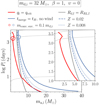 |
Fig. 12. Same as Fig. 5, but illustrating the impact of wind mass loss after the phase of stable MT. The dashed (dotted) blue line shows the modified delay time boundary (solid blue) due to wind mass loss effects, in an environment with Z = 0.02 (Z = 0.008), on the post-MT mass of the stripped star and on the orbital separation at the start of the inspiral phase (see text in Sect. 3.4 for more details). It is important to note that we are considering the effect under the isotropic re-emission β = 1 assumption on the MT episode. For the rest, analogous symbols and notation to Fig. 5 are employed. |
This test case shows that the effect of wind mass loss physics on our results can be impactful, at least in the cases of massive donors (md, i ≳ 10 M⊙) in Milky Way-like environments. We thus reserve a more extensive investigation of winds for future work.
3.5. Including conservativeness ϵ > 0
So far we have carried out our calculations assuming completely non-conservative MT, either in the isotropic re-emission channel with β = 1 and ϵ = 1 − β = 0 (Sect. 2.2), or with a L2 mass outflow with β + υ = 1 and ϵ = 1 − β − υ = 0 (Sect. 2.6). We want to quantify the impact of including an efficiency ϵ > 0 in our calculations of the GW merger boundaries. To this purpose, we are not considering here the additional source of loss from L2, and therefore the efficiency for conservative MT is such that ϵ = 1 − β.
Both the common envelope and the time delay boundaries are expected to change when conservative MT plays a role. The Roche lobe mass-radius exponent is expected to vary smoothly between the limiting cases of β = 1 (Eq. (14)) and ϵ = 1 (Eq. (11)), and is described in Eq. (13). In Fig. 3, this translates into a smooth variation between the solid blue line (isotropic re-emission) and the solid golden line (fully conservative). As a consequence, a shift in critical mass ratios is also expected. In practice, we derived the modified critical mass ratios,  , by solving
 (28)
(28)
On the other hand, the period shrinkage (or widening) Pf/Pi is also modified, varying smoothly between Eq. (5) and the conservative limit (see, e.g., Eq. (33) in Soberman et al. 1997). By solving the equation of angular momentum balance, one can find
 (29)
(29)
where the final mass ratio q = md, f/ma, f takes into account that the final accretor mass is
 (30)
(30)
Lastly, the boundary for Rd, f ≤ RRL, f depends on the amount of shrinkage (widening) of the orbit, and thus is also affected. In Fig. 13 we show the results of our calculations for a donor star of md, i = 32 M⊙. We discretely varied the efficiencies for isotropic re-emission β = 0, 0.5, 1 and conservative MT ϵ = 1 − β. Including conservativeness leads to less shrinkage (and / or widening, if the mass-ratio inversion is reached) of the orbit at the end of the MT episode; on the other hand, the accretor retains some transferred mass, so that the final binary is more massive. This explains the cut in parameter space at the longer initial periods, log Pi > 1.5, and the turnover of the delay time boundary (blue lines) at ∼15 M⊙. Additionally, the Roche lobe boundary Rd, f < RRL, f becomes less stringent as the shrinkage is less extreme, and the instability boundary is mainly affected at the larger accretor masses, where the shift in  is larger (see Fig. 3, top panel).
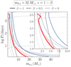 |
Fig. 13. Same as Fig. 5, but illustrating the impact of conservative MT. Boundaries are shown for the case of full isotropic re-emission, with ϵ = 0 (solid line), ϵ = 0.5 (dashed line) and ϵ = 1 (dotted line). The efficiency of isotropic re-emission and conservativeness are varied such that ϵ = 1 − β. |
Although we find that conservative MT can still produce merging binary BHs, the situation is different for donor stars that produce NSs and WDs. The same analysis done for those lower mass donors indicate that the favorable strip for GW formation vanishes for all possible orbital periods. This implies that understanding the conservativeness of MT with CO accretors is critical.
4. Comparison with observations
4.1. Single-degenerate binaries
Even if we expect a set of conditions for a single-degenerate system to lead to coalescing COs, it is not a given that those conditions are realized in nature. Whether the CO + star systems studied in Sect. 3 are formed depends on the evolution of the initially more massive star and its potential interaction with its companion before the formation of the first CO of the system. To check for the existence of the necessary conditions in the single-degenerate stage, we compared the properties of known systems at the CO + star stage to our theoretical predictions of GW progenitors’ initial properties.
To this purpose, we compiled data of known CO + star systems from the literature. For the high mass (X-ray) binaries (HM(XR)Bs) with BHs we collect the data for the six known systems with characterized orbital properties and masses: HD 96670 (Gomez & Grindlay 2021), M33 X-7 (Pietsch et al. 2006; Orosz et al. 2007), LMC X-1 (Mark et al. 1969; Hutchings et al. 1983, 1987), Cyg X-1 (Miller-Jones et al. 2021), VFTS 243 (Shenar et al. 2022) and HD 130298 (Mahy et al. 2022; see Table 1 for a summary of these systems’ properties). In this context, we call mstar the mass of the optical companion to the CO, mCO.
Summary of the six known HM(XR)Bs with BHs.
For HM(XR)Bs with NSs, we considered the galactic systems of Be/X-ray binaries where the CO is a NS, of which a sample of 60–80 is known in the Milky Way (Reig 2011). We collected the data listed in Table 1 of Tomsick & Muterspaugh (2010), which summarizes the sample with estimates of the Be star masses, mstar. To compute the ratio, mCO/mstar, of the NS mass versus the mass of the optical companion, we adopted the reference values for the masses shown in Tomsick & Muterspaugh (2010), without accounting for their uncertainties.
For low mass X-ray binaries (LM(XR)Bs), multiple examples exist, in the literature, with WD objects as accretors. However, these are Roche lobe-filling/strongly interacting systems (e.g., cataclysmic variables, Ritter & Kolb 2003 or classical novae, Darnley et al. 2004) where the current mass of the donor star does not represent its pre-interaction properties required in our analysis. Determinations of masses and periods for detached single-degenerate binaries with WDs are not commonly found in the literature. We first considered systems composed by a WD + MS star with determined orbital properties: the Zwicky Transient Facility (ZTF) catalogue by Brown et al. (2023) of ZTF systems (MS companions of spectral type M or later), and the compilation by Holberg et al. (2013) of Sirius-like systems (MS companions of spectral type K or earlier). We then considered systems composed of hot subdwarf stars of spectral type B or O (sdB/O) + MS companions (named ELCVNs after the prototype system, Maxted et al. 2011) and binaries with sdO + Be stars companions. These systems are assumed to be representative of a non-interacting stage preceding the single-degenerate configuration, as the subdwarf star is expected to evolve into a Helium WD. ELCVNs with determined mass ratios and orbital periods were taken from the catalogues in van Roestel et al. (2018; their Table A4.2) and Maxted et al. (2014; their Table 2). To these, we added ten systems found in the Kepler survey, with references in van Roestel et al. (2018). For sdO + Be/Xray stars, we used the compilation in Wang et al. (2023; Table 9). In each of these cases, we took the reference values for q and Porb without uncertainties.
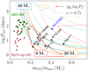 |
Fig. 14. Observed orbital periods, log Porb, and mass ratios, i.e. mCO/mstar, for high (and intermediate) mass X-ray binaries and quiescent OB + BH systems. The markers report data points (uncertainties are neglected) listed in a) Table 1 for HM(XR)Bs with BHs (black stars), with the corresponding labeled names, and b) Table 1 from Tomsick & Muterspaugh (2010) for HM(XR)Bs with NS (red stars). We also report the Casares et al. (2014) system (blue star). The triangles show the sample of confirmed sdO + Be stars in Table 9 of Wang et al. (2023). The solid, colored contours are the correspondent loci predicted by our calculations to be promising for GW progenitor systems via stable MT, within the assumption of purely isotropic re-emission, β = 1. Every contour is labeled with the associated fixed donor’s initial mass, md, i. The dotted, colored contours show the same loci (md, i/ma, i, log Pi) within the assumption of an efficiency for mass outflow via L2 such that υ = 0.5. |
Figure 14 shows the comparison between our theoretical predictions of the conditions needed to form a GW source (solid lines) and the six known HM(XR)Bs with BHs together with the considered sample of Be stars orbiting NSs and sdO + Be binaries (single markers). The population of HM(XR)Bs with BHs extends within 0 ≲ log Porb(day)≲1. The population of Be-Xray binaries with NSs lies within 0.05 ≤ mCO/mstar ≤ 0.18, with mass ratios for which we predict MT to be unstable. Similarly, the sample of sdO + Be stars lies in the unstable MT region (see also Fig. 15), spanning larger periods, 1.5 ≲ log Porb(day)≲2.5. The lack of lower-mass Be stars in X-ray binaries (barring uncertainties in mass determinations from spectral types) has been used to argue for efficient MT in binary systems before the formation of the first CO (Vinciguerra et al. 2020). In this context, efficient MT is able to preclude the formation of Be/X-ray binaries with higher mass ratios than the ones that would evolve stably and form merging binary NSs. Conservative MT prior to the first CO formation has also been advanced as an explanation for the evolutionary stage of some sdO + Be star systems (e.g., HR6819, Bodensteiner et al. 2020). As for Be/X-ray systems with BHs, only one candidate is known, HD 215227 (MWC 656, Casares et al. 2014), also reported in Fig. 14. However, this system might contain a hot subdwarf object orbiting the Be-star (Rivinius et al. 2022).
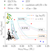 |
Fig. 15. Observed orbital periods, log Porb, and mass ratios, mCO/mstar, for low (and intermediate) mass single-degenerate binaries. More specifically: WD + MS stars from the ZTF catalogue of Brown et al. (2023; ZTF) and Holberg et al. (2013; Sirius-like); sdO/B + MS stars from van Roestel et al. (2018), Maxted et al. (2014) and ten Kepler systems (see main text); sdO/B + Be stars, which are separated into candidate systems (candidate sdO/B + Be), confirmed sdO + Be, and γCas-like systems, as in Wang et al. (2023). Markers report the reference data points without uncertainties. Solid, colored contours are the correspondent loci predicted by our calculations to be promising for GW progenitor systems via stable MT and follow the same notation as in Fig. 14. |
Figure 14 shows also the results of switching on an efficiency for mass outflow from L2 of υ = 0.75 (dashed lines). The predicted regions for GW progenitors’ parameter space are consistently shifted toward more extreme mass ratios in an area that is not yet populated by known observations of CO + star binaries prior to the remaining star filling its Roche lobe. HD 215227 is the only system within the region with a massive donor predicted to directly collapse into a BH (the representative contour being the one for md, i = 40 M⊙) and at the same time close to the predicted region for a NS remnant (the representative contour being the one for md, i = 20 M⊙).
Assuming that the post-MT state and the final fate of the optical companions for HM(XR)Bs are described by those of our theoretical results for the closest initial donor’s mass found in the Ge et al. (2020) table, we can assess if the conditions for the stable MT channel to produce a GW source are realized in nature. Some of these systems, however, present a non-negligible eccentricity (see Table 1). Our predictions, on the other hand, assume that, at the stage of the Roche lobe-filling donor, the CO + star system is already circular (we use Kepler’s third law in the form of Eq. (16)). To compare with our results for circular orbits we assume that, near the onset of Roche lobe overflow, the orbit circularizes to a period,  , such that
 (31)
(31)
resulting from the preservation of orbital angular momentum. For e we used the values of the observed eccentricities in Table 1. We then associated each mstar with the closest initial donor’s mass in our simulation set,  . We finally made a comparison, in Fig. 14, of the systems with the theoretical contours for different
  .
.
Table 2 summarizes the predicted evolution (or outcome) of the known systems with BHs, based on our purely isotropic re-emission, β = 1, and mass outflow from L2, υ = 0.75, evolutionary channels. We report the associated initial donor’s mass in the Ge et al. (2020) data and the modeled fate of the second-born CO. Lastly, we tabulate whether the systems have a set of initial properties that can lead to the evolution into merging double COs via stable MT (GW merger), or whether they are expected to evolve into a wide binary or undergo unstable MT.
Predicted outcome of the second-born (2nd) CO for the known HM(XR)Bs with BHs.
Barring the limitations of this comparison, for the isotropic re-emission case, β = 1, we find systems covering all outcomes, including unstable MT, the formation of wide CO + CO systems and merging CO + CO expected to undergo stable MT (i.e., they appear within their associated theoretical contours in Fig. 14). This provides support for the idea that the conditions for the stable MT channel are realized in nature, provided that we neglect stellar winds widening the orbit after interaction (see Sect. 3.4). Interestingly, HD 96670 presents conditions that can be compatible with the formation of a NS-BH merger. Considering cases with L2 mass outflow, υ > 0, the conditions for forming a GW source shift to larger CO masses, mCO. In particular, for υ = 0.75 we find that only MWC 656 (for which the presence of a BH is contested, Rivinius et al. 2022) is compatible with the formation of a GW source. We also notice that two systems, VFTS 243 and M33 X-7, do not show in Fig. 14 suitable properties for being GW progenitor systems via stable MT with either β = 1 or with υ = 0.75. For VFTS 243, however, we can find a GW merger outcome via stable MT by switching on an efficiency for L2 such that 0.25 ≲ υ ≲ 0.5 (see Fig. 6).
We show in Fig. 15 the same comparison as in Fig. 14 between our theoretical predictions and the compilation of LM(XR)Bs and single-degenerate representative systems collected from literature (colored markers). The systems with sdO + Be stars are separated into candidate systems (candidate sdO/B + Be) from optical spectroscopy and confirmed sdO + Be and γCas-like systems (from the prototype Secchi 1866); see Table 9 in Wang et al. (2023) for the distinction. For the single-degenerate binaries WD + MS, consistent biases toward small orbital period (log Porb < 0) binaries (as well as low mass for the MS companion) are present in photometric surveys such as ZTF. On the other hand, Sirius-like systems are usually best resolved with proper motion surveys, causing biases toward the wide orbits (mostly with log Porb > 3). The sample of ELCVNs and sdB/O + Be/Xray stars extends within −0.1 ≲ log Porb(day)≲2.5 and mostly encompasses mass ratios for which we predict MT to be unstable. This holds true whether or not additional L2 momentum loss is accounted for (dotted lines). The degenerate companions in ELCVNs systems are generally very low mass (∼0.2 M⊙) pre-Helium WDs, but more massive companions could shift the populated region to that predicted by us for GW mergers via stable MT.
4.2. Compact object mergers
We want to compare the GWTC-3 information with the results from our simulation set for the mass ratios, qf, and the total mass, mf = ma, f + αcoremd, i, achievable after the stable MT episode. To this purpose, Fig. 16 compares the total mass and mass ratios of detected CO mergers against our predictions for stable MT. Together with the results from our study, we show the 90% density interval as the credible region for some representative systems to illustrate the uncertainties in the total mass and mass ratios of the GW observations.
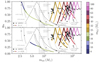 |
Fig. 16. Plane of final mass ratio qfin < 1 and total final mass, mtot. We report the estimation values with corresponding 90% credible intervals for the GWTC-3 signal (gray/black dots) and the posterior 90% iso-contour for a selection of those (gray dots and light gray curves). Resulting final mass ratios and total mass from our treatment are reported with color coding referring to different donor masses md, i in the simulation grid from Ge et al. series Ge et al. (2020), 2015, 2010). The assumption of completely non-conservative, purely isotropic re-emission, β = 1, channel is adopted in the top panel, while the bottom panel shows the results when switching on an efficiency for L2 mass outflow of υ = 0.75. Solid gray, dashed lines delineate regions where the primary and secondary can have a mass below 3 M⊙, and where both objects in the binary have masses above 3 M⊙. |
We notice a difference in the (mtot, qfin) shapes between the donor masses in the range of BH progenitors, namely md, i ≳ 20 M⊙, and the ones in the range of NS progenitors, i.e. 8 ≲ md, i/M⊙ ≲ 20. As for the BH progenitors, for each given donor mass the shape extends till qfin = 1, showing again that for all such donors the second-born CO could be either the more massive one (which happens at longer initial periods, Pi, see e.g., Fig. 6), or the less massive one (happening, conversely, at smaller initial periods, Pi in Fig. 6). For the NS progenitors, the shape does not reach the unitary final mass ratio (aside from a small portion of points in the case of md, i = 8 M⊙) because we assumed that the post-SN object would have a canonical mass of 1.4 M⊙ (see Sect. 3.2), resulting in a final mass ratio qf = 1.4/ma, f mostly such that qf < 1. Therefore, if the second-born CO is a NS (i.e., coming from a SN explosion of a donor star such that 8 ≲ md, i/M⊙ ≲ 20) of canonical mass, it will most likely be the less massive object in the CO + CO pair.
We also observe that the stable MT channel, in the purely isotropic re-emission limit, has the potential to reproduce the final properties of the majority of GWTC-3 signals, in terms of final mass ratios and thetotal mass of the mergers. Covered mass ratios are such that qfin ≳ 0.1. On the other hand, our predictions cover the full range of final total masses mtot (although we do not include the effect of pair instability SNe in our treatment of BH progenitors, which could limit the possible ranges). Notable exceptions are GW191219-163120, which stands at  and
and  ; GW200210-092254 at
  and
and  ; GW190814 at
  and
and  .
.
Including higher angular momentum loss by switching on an efficiency υ > 0 for L2 outflow (Fig. 16, bottom) results in less extreme final mass ratios (qfin ≳ 0.25 for υ = 0.75, as opposed to qfin ≳ 0.1 for β = 1) coming from merging binary BHs, and no possible path to the formation of a merging binary NSs from stable mass transfer (see Sect. 3.2). This is due to the common envelope boundary being shifted to smaller final mass ratios, qf, at the end of the MT episode, making any MT event from a hydrogen rich NS progenitor onto a NS unstable (see e.g., Fig. 8).
An important limitation of this comparison with the population of observed GWTC-3 CO + CO mergers comes from the fact that we are not considering the information on spins. The high inferred BH spins in HM(XR)Bs have been used to argue that they are subdominant progenitors of the observed population of binary BH mergers (e.g., Fishbach & Kalogera 2022; Gallegos-Garcia et al. 2022), while others think that spin measurements in HM(XB)s should be taken with care (Belczynski et al. 2021). Among the models that attempt to explain the near critical spins inferred for HM(XR)Bs, one idea is that the spin is inherited from their progenitor star being tidally locked in a short period orbit during its main sequence (Valsecchi et al. 2010; Qin et al. 2019). If this were the case, longer period OB + BH systems would be expected to have lower BH spins potentially consistent with the observed binary BH population. The detections of VFTS 243 (Shenar et al. 2022) and HD 130298 (Mahy et al. 2022) have started to probe these longer orbital periods and the Gaia mission is expected to provide hundreds of additional detections in this regime (e.g., Breivik et al. 2017; Mashian & Loeb 2017; Wiktorowicz et al. 2019; Janssens et al. 2022, 2023). However, such wide systems are expected to lack accretion disks (Sen et al. 2021; Hirai & Mandel 2021), making it impossible to apply current methods to measuring BH spins.
5. Conclusions
We studied the parameter space of the initial properties of systems composed of a first-born CO orbiting a Roche lobe-filling donor. At an arbitrary evolutionary stage, the system is expected to undergo a stable MT episode and, after the formation of the second-born CO, to evolve into a double CO configuration able to merge within a Hubble time. We summarize our main findings in the following:
-
Under the assumption of fully non-conservative MT and isotropic re-emission from the accreting CO, we find that stable MT can produce all possible pairings of merging double COs except for WD + BH binaries. This holds, barring limitations on the properties (masses and orbital periods) of single-degenerate binaries that arise from the evolution until the formation of the first CO.
-
The possible formation of NS + NS mergers from stable MT is limited to a narrow range in the initial properties. For a typical NS mass of 1.4 M⊙, any companion massive enough to form a second-born NS (md, i ≳ 8 M⊙) will have an extreme mass ratio, such that binary NSs can only be produced in a narrow range of donor masses and orbital periods.
-
Including additional angular momentum loss (by considering a fraction of the mass removing the angular momentum corresponding to L2), the initial orbital periods suitable for GW mergers via stable MT are shifted toward larger initial mass ratios q = md, i/ma, i. Such additional angular momentum loss can prevent stable MT from forming merging binary NSs. On the other hand, the inclusion of L2 mass outflow with efficiency ≥ 50% can allow a WD + BH pair to merge within the age of the universe.
-
We compared our results with observations of single-degenerate binaries, that is, HM(XR)Bs with black holes and Be-Xray binaries with NSs. For the isotropic re-emission calculations, the conditions required for the stable MT channel to operate seem to be present in nature. In particular, the candidate BH system HD 96670 (Gomez & Grindlay 2021) has properties consistent with the formation of a merging NS + BH. As future (and current) surveys are expected to unveil more high-mass BHs, in particular the wider-orbit counterparts to BH companions and the lower-mass optical companions to NS, we can expect to observe more systems showing such favorable conditions.
-
Considering isotropic re-emission, stable MT can produce merging binary BHs with mass ratios q ≥ 0.1. This covers the majority of the sources observed in the GWTC-3 catalogue, except for extreme cases such as GW190814. Considering enhanced angular momentum loss limits the minimum mass ratios that can be achieved. In particular, under the assumption that 75% of the material is removed with the angular momentum of the L2 point, we do not find BH mergers with q < 0.25.
We have made our results available to the community in tabular, machine-readable form on Zenodo2: tables at fixed donor mass, md, i, listing the boundaries (ma, i, log Pi) of GW progenitor systems at different efficiencies of angular momentum loss, i.e. varying discretely β ∈ [0, 1] and υ ∈ [0, 1] and keeping the total efficiency ϵ = β + υ = 1. Modified boundaries with some degree of conservativeness are also provided in the case ϵ = 1 − β, for β = 0, 0.5, 1.
Our work provides a simple, semi-analytical approach to studying the physics and limitations of the stable MT channel. We therefore implicitly assume the existence of specific configurations of CO + star systems. Although we have shown that a comparison to known systems in that intermediate stage is promising, it is important to validate our results using detailed binary evolution calculations, which we aim to do in future work. Simulations starting from two stars at the ZAMS, rather than after the formation of the first CO, are also necessary to determine the formation rates of these systems (e.g., Bavera et al. 2021; Gallegos-Garcia et al. 2021) and compare them to observed rates of CO coalescences. Detailed simulations can also show the impact of a previous MT phase on the donor star in a CO + star system, which will modify its response to MT and thus the MT stability itself.
https://zenodo.org/records/8334057
https://zenodo.org/records/8334057
Acknowledgments
A.P. acknowledges support from the FWO PhD fellowship fundamental research under project 11M8323N and the Interuniversity BOF project No. 20-VLIR-iBOF-021. P.M. acknowledges support from the FWO junior postdoctoral fellowship No. 12ZY520N and the FWO senior postdoctoral fellowship No. 12ZY523N. This project has received funding from the European Research Council (ERC) under the European Union’s Horizon 2020 research and innovation programme (grant agreement No. 772225/MULTIPLES). G.N. acknowledges support form the Dutch Science Foundation NWO.
References
- Abbott, R., Abbott, T. D., Acernese, F., et al. 2023, Phys. Rev. X, 13, 041039 [Google Scholar]
- Amaro-Seoane, P., Audley, H., Babak, S., et al. 2017, ArXiv e-prints [arXiv:1702.00786] [Google Scholar]
- Atri, P., Miller-Jones, J. C. A., Bahramian, A., et al. 2019, MNRAS, 489, 3116 [NASA ADS] [CrossRef] [Google Scholar]
- Bavera, S. S., Fragos, T., Zevin, M., et al. 2021, A&A, 647, A153 [NASA ADS] [CrossRef] [EDP Sciences] [Google Scholar]
- Belczynski, K., Holz, D. E., Bulik, T., & O’Shaughnessy, R. 2016, Nature, 534, 512 [NASA ADS] [CrossRef] [Google Scholar]
- Belczynski, K., Done, C., & Lasota, J. P. 2021, ArXiv e-prints [arXiv:2111.09401] [Google Scholar]
- Bodensteiner, J., Shenar, T., Mahy, L., et al. 2020, A&A, 641, A43 [NASA ADS] [CrossRef] [EDP Sciences] [Google Scholar]
- Brandt, N., & Podsiadlowski, P. 1995, MNRAS, 274, 461 [NASA ADS] [CrossRef] [Google Scholar]
- Breivik, K., Chatterjee, S., & Larson, S. L. 2017, ApJ, 850, L13 [CrossRef] [Google Scholar]
- Brown, A. J., Parsons, S. G., van Roestel, J., et al. 2023, MNRAS, 521, 1880 [NASA ADS] [CrossRef] [Google Scholar]
- Casares, J., Negueruela, I., Ribó, M., et al. 2014, Nature, 505, 378 [Google Scholar]
- Cassisi, S., Iben, Icko Jr., & Tornambè, A., 1998, ApJ, 496, 376 [NASA ADS] [CrossRef] [Google Scholar]
- Chau, W. Y., Henriksen, R. N., & Alexander, M. E. 1974, BAAS, 6, 488 [NASA ADS] [Google Scholar]
- Darnley, M. J., Bode, M. F., Kerins, E., et al. 2004, MNRAS, 353, 571 [NASA ADS] [CrossRef] [Google Scholar]
- Dominik, M., Belczynski, K., Fryer, C., et al. 2012, ApJ, 759, 52 [Google Scholar]
- Eggleton, P. P. 1983, ApJ, 268, 368 [Google Scholar]
- Fabrika, S. N. 1993, MNRAS, 261, 241 [NASA ADS] [Google Scholar]
- Fishbach, M., & Kalogera, V. 2022, ApJ, 929, L26 [NASA ADS] [CrossRef] [Google Scholar]
- Fryer, C. L. 1999, ApJ, 522, 413 [NASA ADS] [CrossRef] [Google Scholar]
- Gallegos-Garcia, M., Berry, C. P. L., Marchant, P., & Kalogera, V. 2021, ApJ, 922, 110 [NASA ADS] [CrossRef] [Google Scholar]
- Gallegos-Garcia, M., Fishbach, M., Kalogera, V., Berry, C. P., & Doctor, Z. 2022, ApJ, 938, L19 [NASA ADS] [CrossRef] [Google Scholar]
- Ge, H., Hjellming, M. S., Webbink, R. F., Chen, X., & Han, Z. 2010, ApJ, 717, 724 [NASA ADS] [CrossRef] [Google Scholar]
- Ge, H., Webbink, R. F., Chen, X., & Han, Z. 2015, ApJ, 812, 40 [Google Scholar]
- Ge, H., Webbink, R. F., Chen, X., & Han, Z. 2020, ApJ, 899, 132 [NASA ADS] [CrossRef] [Google Scholar]
- Gomez, S., & Grindlay, J. E. 2021, ApJ, 913, 48 [NASA ADS] [CrossRef] [Google Scholar]
- Hall, E. D., & Evans, M. 2019, CQG, 36, 225002 [NASA ADS] [CrossRef] [Google Scholar]
- Hills, J. G. 1983, ApJ, 267, 322 [NASA ADS] [CrossRef] [Google Scholar]
- Hirai, R., & Mandel, I. 2021, PASA, 38, e056 [NASA ADS] [CrossRef] [Google Scholar]
- Hjellming, M. S., & Webbink, R. F. 1987, ApJ, 318, 794 [Google Scholar]
- Hobbs, G., Lorimer, D. R., Lyne, A. G., & Kramer, M. 2005, MNRAS, 360, 974 [Google Scholar]
- Holberg, J. B., Oswalt, T. D., Sion, E. M., Barstow, M. A., & Burleigh, M. R. 2013, MNRAS, 435, 2077 [Google Scholar]
- Humphreys, R. M., & Davidson, K. 1979, ApJ, 232, 409 [Google Scholar]
- Hurley, J. R., Tout, C. A., & Pols, O. R. 2002, MNRAS, 329, 897 [Google Scholar]
- Hutchings, J. B., Crampton, D., & Cowley, A. P. 1983, ApJ, 275, L43 [NASA ADS] [CrossRef] [Google Scholar]
- Hutchings, J. B., Crampton, D., Cowley, A. P., Bianchi, L., & Thompson, I. B. 1987, AJ, 94, 340 [NASA ADS] [CrossRef] [Google Scholar]
- Iben, I. Jr., & Tutukov, A. V. 1984, ApJS, 54, 335 [NASA ADS] [CrossRef] [Google Scholar]
- Janssens, S., Shenar, T., Sana, H., et al. 2022, A&A, 658, A129 [NASA ADS] [CrossRef] [EDP Sciences] [Google Scholar]
- Janssens, S., Shenar, T., Sana, H., & Marchant, P. 2023, A&A, 670, A79 [NASA ADS] [CrossRef] [EDP Sciences] [Google Scholar]
- Kalogera, V. 1996, ApJ, 471, 352 [Google Scholar]
- Kulkarni, S. R., Hut, P., & McMillan, S. 1993, Nature, 364, 421 [Google Scholar]
- Lai, D., Chernoff, D. F., & Cordes, J. M. 2001, ApJ, 549, 1111 [NASA ADS] [CrossRef] [Google Scholar]
- Langer, N. 2012, ARA&A, 50, 107 [CrossRef] [Google Scholar]
- Langer, N., Schürmann, C., Stoll, K., et al. 2020, A&A, 638, A39 [NASA ADS] [CrossRef] [EDP Sciences] [Google Scholar]
- Liu, W. M., Yungelson, L., & Kuranov, A. 2022, A&A, 668, A80 [NASA ADS] [CrossRef] [EDP Sciences] [Google Scholar]
- Lu, W., Fuller, J., Quataert, E., & Bonnerot, C. 2023, MNRAS, 519, 1409 [Google Scholar]
- Mabanta, Q. A., Murphy, J. W., & Dolence, J. C. 2019, ApJ, 887, 43 [NASA ADS] [CrossRef] [Google Scholar]
- Maggiore, M., Van Den Broeck, C., Bartolo, N., et al. 2020, JCAP, 2020, 050 [CrossRef] [Google Scholar]
- Mahy, L., Sana, H., Shenar, T., et al. 2022, A&A, 664, A159 [NASA ADS] [CrossRef] [EDP Sciences] [Google Scholar]
- Mandel, I., & De Mink, S. 2016, in 41st COSPAR Scientific Assembly, 41, E1.16-13-16 [Google Scholar]
- Mapelli, M. 2016, MNRAS, 459, 3432 [NASA ADS] [CrossRef] [Google Scholar]
- Marchant, P., Langer, N., Podsiadlowski, P., Tauris, T. M., & Moriya, T. J. 2016, A&A, 588, A50 [NASA ADS] [CrossRef] [EDP Sciences] [Google Scholar]
- Marchant, P., Pappas, K. M. W., Gallegos-Garcia, M., et al. 2021, A&A, 650, A107 [NASA ADS] [CrossRef] [EDP Sciences] [Google Scholar]
- Mark, H., Price, R., Rodrigues, R., Seward, F. D., & Swift, C. D. 1969, ApJ, 155, L143 [NASA ADS] [CrossRef] [Google Scholar]
- Mashian, N., & Loeb, A. 2017, MNRAS, 470, 2611 [NASA ADS] [CrossRef] [Google Scholar]
- Maxted, P. F. L., Anderson, D. R., Burleigh, M. R., et al. 2011, MNRAS, 418, 1156 [NASA ADS] [CrossRef] [Google Scholar]
- Maxted, P. F. L., Bloemen, S., Heber, U., et al. 2014, MNRAS, 437, 1681 [NASA ADS] [CrossRef] [Google Scholar]
- Miller-Jones, J. C. A., Bahramian, A., Orosz, J. A., et al. 2021, Science, 371, 1046 [Google Scholar]
- Müller, B., Heger, A., Liptai, D., & Cameron, J. B. 2016, MNRAS, 460, 742 [Google Scholar]
- Neijssel, C. J., Vigna-Gómez, A., Stevenson, S., et al. 2019, MNRAS, 490, 3740 [Google Scholar]
- Nomoto, K. 1982, ApJ, 253, 798 [Google Scholar]
- O’Connor, E., & Ott, C. D. 2011, ApJ, 730, 70 [Google Scholar]
- Orosz, J. A., McClintock, J. E., Narayan, R., et al. 2007, Nature, 449, 872 [NASA ADS] [CrossRef] [Google Scholar]
- Orosz, J. A., Steeghs, D., McClintock, J. E., et al. 2009, ApJ, 697, 573 [NASA ADS] [CrossRef] [Google Scholar]
- Paczyński, B. 1965, Acta. Astron., 15, 89 [Google Scholar]
- Paczynski, B. 1976, in Structure and Evolution of Close Binary Systems, eds. P. Eggleton, S. Mitton, & J. Whelan, 73, 75 [NASA ADS] [CrossRef] [Google Scholar]
- Pavlovskii, K., & Ivanova, N. 2015, MNRAS, 449, 4415 [Google Scholar]
- Paxton, B., Bildsten, L., Dotter, A., et al. 2010, Astrophysics Source Code Library [record ascl:1010.083] [Google Scholar]
- Paxton, B., Cantiello, M., Arras, P., et al. 2013, ApJS, 208, 4 [Google Scholar]
- Paxton, B., Marchant, P., Schwab, J., et al. 2015, ApJS, 220, 15 [Google Scholar]
- Paxton, B., Schwab, J., Bauer, E. B., et al. 2018, ApJS, 234, 34 [NASA ADS] [CrossRef] [Google Scholar]
- Paxton, B., Smolec, R., Schwab, J., et al. 2019, ApJS, 243, 10 [Google Scholar]
- Peters, P. C. 1964, Phys. Rev., 136, B1224 [NASA ADS] [CrossRef] [Google Scholar]
- Pietsch, W., Haberl, F., Sasaki, M., et al. 2006, ApJ, 646, 420 [NASA ADS] [CrossRef] [Google Scholar]
- Poelarends, A. J. T., Herwig, F., Langer, N., & Heger, A. 2008, ApJ, 675, 614 [Google Scholar]
- Poniatowski, L. G., Sundqvist, J. O., Kee, N. D., et al. 2021, A&A, 647, A151 [NASA ADS] [CrossRef] [EDP Sciences] [Google Scholar]
- Portegies Zwart, S. F., & McMillan, S. L. W. 2000, ApJ, 528, L17 [Google Scholar]
- Qin, Y., Marchant, P., Fragos, T., Meynet, G., & Kalogera, V. 2019, ApJ, 870, L18 [Google Scholar]
- Reig, P. 2011, Ap&SS, 332, 1 [Google Scholar]
- Ritter, H., & Kolb, U. 2003, A&A, 404, 301 [NASA ADS] [CrossRef] [EDP Sciences] [Google Scholar]
- Rivinius, T., Klement, R., Chojnowski, S. D., et al. 2022, ArXiv e-prints [arXiv:2208.12315] [Google Scholar]
- Sander, A. A. C., & Vink, J. S. 2020, MNRAS, 499, 873 [Google Scholar]
- Secchi, A. 1866, Astron. Nachr., 68, 63 [Google Scholar]
- Sen, K., Xu, X. T., Langer, N., et al. 2021, A&A, 652, A138 [NASA ADS] [CrossRef] [EDP Sciences] [Google Scholar]
- Shen, K. J., & Bildsten, L. 2007, ApJ, 660, 1444 [NASA ADS] [CrossRef] [Google Scholar]
- Shenar, T., Sana, H., Mahy, L., et al. 2022, Nat. Astron., 6, 1085 [NASA ADS] [CrossRef] [Google Scholar]
- Sigurdsson, S., & Hernquist, L. 1993, Nature, 364, 423 [Google Scholar]
- Soberman, G. E., Phinney, E. S., & van den Heuvel, E. P. J. 1997, A&A, 327, 620 [NASA ADS] [Google Scholar]
- Sparks, W. M., & Stecher, T. P. 1974, ApJ, 188, 149 [NASA ADS] [CrossRef] [Google Scholar]
- Spera, M., Mapelli, M., & Bressan, A. 2015, MNRAS, 451, 4086 [NASA ADS] [CrossRef] [Google Scholar]
- Sutantyo, W. 1978, Ap&SS, 54, 479 [NASA ADS] [CrossRef] [Google Scholar]
- Tauris, T. M., Fender, R. P., van den Heuvel, E. P. J., Johnston, H. M., & Wu, K. 1999, MNRAS, 310, 1165 [NASA ADS] [CrossRef] [Google Scholar]
- Tauris, T. M., Kramer, M., Freire, P. C. C., et al. 2017, ApJ, 846, 170 [Google Scholar]
- Thompson, T. A. 2011, ApJ, 741, 82 [NASA ADS] [CrossRef] [Google Scholar]
- Tomsick, J. A., & Muterspaugh, M. W. 2010, ApJ, 719, 958 [NASA ADS] [CrossRef] [Google Scholar]
- Ugliano, M., Janka, H.-T., Marek, A., & Arcones, A. 2012, ApJ, 757, 69 [NASA ADS] [CrossRef] [Google Scholar]
- Valsecchi, F., Glebbeek, E., Farr, W. M., et al. 2010, Nature, 468, 77 [NASA ADS] [CrossRef] [Google Scholar]
- van den Heuvel, E. P. J. 1976, in Structure and Evolution of Close Binary Systems, eds. P. Eggleton, S. Mitton, & J. Whelan, 73, 35 [Google Scholar]
- van den Heuvel, E. P. J., Zwart, S. F. P., & de Mink, S. E. 2017, MNRAS, 471, 4256 [NASA ADS] [CrossRef] [Google Scholar]
- van Roestel, J., Kupfer, T., Ruiz-Carmona, R., et al. 2018, MNRAS, 475, 2560 [CrossRef] [Google Scholar]
- Verbunt, F., Wijers, R. A. M. J., & Burm, H. M. G. 1990, A&A, 234, 195 [NASA ADS] [Google Scholar]
- Vinciguerra, S., Neijssel, C. J., Vigna-Gómez, A., et al. 2020, MNRAS, 498, 4705 [NASA ADS] [CrossRef] [Google Scholar]
- Wang, L., Gies, D. R., Peters, G. J., & Han, Z. 2023, AJ, 165, 203 [NASA ADS] [CrossRef] [Google Scholar]
- Webbink, R. F. 1975, PhD Thesis, University of Cambridge, UK [Google Scholar]
- Webbink, R. F. 1984, ApJ, 277, 355 [NASA ADS] [CrossRef] [Google Scholar]
- Wellstein, S., Langer, N., & Braun, H. 2001, A&A, 369, 939 [NASA ADS] [CrossRef] [EDP Sciences] [Google Scholar]
- Wiktorowicz, G., Wyrzykowski, Ł., Chruslinska, M., et al. 2019, ApJ, 885, 1 [NASA ADS] [CrossRef] [Google Scholar]
- Wolf, W. M., Bildsten, L., Brooks, J., & Paxton, B. 2013, ApJ, 777, 136 [Google Scholar]
Appendix A: L2 calculations
To determine the change in orbital period due to an outflow from the L2 point one needs to compute the integral (see Section 2.6)
![Mathematical equation: $$ \begin{aligned} \int _{q_\mathrm{i} }^{q_\mathrm{f} }\frac{1+q}{q}\left[x_{L_2}(q)-x_{\mathrm{cm} }\right]^2 dq=\int _{q_\mathrm{i} }^{q_\mathrm{f} }f(q)\, dq, \end{aligned} $$](/articles/aa/full_html/2024/01/aa47090-23/aa47090-23-eq77.gif) (A.1)
(A.1)
where f(q) is defined as
![Mathematical equation: $$ \begin{aligned} f(q)=&\displaystyle \frac{1+q}{q}\,\left[1+\sum _{n=1}^5 a_n\times {\left\{ \begin{array}{ll} q^{-(n-n_0)}&q\ge 1 \\ q^{(n-n_0)}&q{< }1 \end{array}\right.} \right] \end{aligned} $$](/articles/aa/full_html/2024/01/aa47090-23/aa47090-23-eq78.gif) (A.2)
(A.2)
 (A.3)
(A.3)

In the above we made use of the fit to xL2 − xcm in Eq. 20. We also introduced the functions f≷(q) to describe the piece-wise function f(q) in the mass ratio regimes q ≷ 1, respectively. As the integrand f(q) is a piecewise function, we need to consider different possible outcomes depending on whether or not the binary crosses a mass ratio of unity during the MT event. Let us first consider the indefinite integral, I(q):
 (A.4)
(A.4)
By direct integration we have that
 (A.5)
(A.5)
with
and the coefficients an and n0 are given in Eq. 20. In this expression nmax = 5 and a0 = 0 = an > 5. The result of the definite integral can then be computed as
 (A.6)
(A.6)
Appendix B: Comparison to Marchant et al. (2021) results
As this work serves as a benchmark and is meant to be followed by a detailed set of MESA simulations, we also want to compare our results for a donor of md, i = 32 M⊙ with the ones presently available. To this purpose, we consider the work from Marchant et al. (2021), in which the evolution of a metal-poor (Z = 0.00142) 30 M⊙ donor star orbiting a CO is modeled with MESA. For the comparison, we show in Fig. B.1 the (ma, i/md, i − log Pi) parameter space. Their grid of simulations spans initial orbital periods, Pi, ranging from −0.3 < log Pi(days)< 3.5, and initial mass ratios, ma, i/md, i, between 0.01 and 0.59 (see Sect. 3.1 of their paper for more details on the grid), translating into CO masses 0.3 < ma, i/M⊙ < 17.7.
The delay time boundary computed by us in the isotropic re-emission channel is close to the one found by Marchant et al., in which the degree of non-conservativeness is not a free parameter (i.e., they are not fixing an efficiency, β). The efficiency of MT is instead determined by limiting the accretion rate into the CO by its Eddington limit, with all the surplus material being removed under the assumption of isotropic re-emission. For the 30 M⊙ donor considered by Marchant et al. (2021), MT rates exceed the Eddington limit of the CO by orders of magnitude, resulting in a near-zero efficiency. The simulations of Marchant et al. (2021) also include a treatment for outflows from the outer Lagrangian points (in situations in which the donor grows significantly beyond its Roche lobe); these outflows account for only a small fraction of the total ejected mass (see their figure 13). Considering this, their simulations can be compared to our results with β = 1.
The instability boundary in our study is pushed to lower mass ratios compared to the results of detailed simulations in Marchant et al. (2021). Our instability boundary for md, i = 32 M⊙ is much influenced by the hard limit on RHe − ZAMS < RRL, f (see Sect. 2.5), and a realistic condition can be even more conservative. This apparent discrepancy might therefore attenuate or disappear, once one resolves the boundaries with detailed simulations.
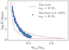 |
Fig. B.1. Parameter space (q0 = ma, i/md, i − log Pi) of GW progenitors initial properties, comparing results from the simulations from (Marchant et al. 2021; blue dots), for a donor of md, i = 30 M⊙ and results from this work (pink contour), for a donor of md, i = 32 M⊙. |
All Tables
All Figures
|
Fig. 1. Locus (see Eq. (8)) for the formation of a GW source through stable MT with a 30 M⊙ donor as a function of the CO accretor mass, ma, i, and orbital period, Pi. The solid curves represent the upper bounds on initial periods log Pi, to achieve a delay time of tmerge = tH; different stripping factors, αcore, are labeled along the corresponding curves. Colored diamonds correspond to the point, along their respective curves, at which the MT episode is expected to invert the mass ratio. |
| In the text | |
|
Fig. 2. Hertzsprung-Russell diagram of the adiabatic mass loss sequences from Ge et al. (2020), labeled by their mass. Different evolutionary phases (TAMS, helium ignition and end of core He-burning) are highlighted with different icons (unfilled triangle, circle, and square). The empirical Humphrey-Davidson (HD) limit, in dashed red (Humphreys & Davidson 1979), is also reported. |
| In the text | |
|
Fig. 3. Functional dependence of ζRL on the binary mass ratio qi ≡ md, i/ma, i, compared to the adiabatic index, ζad, for donor stars of 32 M⊙ (top panel) and 2 M⊙ (bottom panel) of different radii. The different colors of the solid lines show the conservative limit, ϵ = 1 (golden), and the completely non-conservative cases of purely isotropic re-emission, β = 1 (dark blue), and mass outflow from L2 (light blue), see the discussion in Sect. 2.6. Critical mass ratios, ζad, for the MT to be unstable, as calculated by Ge et al. (2020), are shown as horizontal lines (labeled by the donor star radius). For each radius and mode of MT, the critical mass ratio corresponds to the crossing points between ζad and ζRL. |
| In the text | |
|
Fig. 4. Same diagram as in Fig. 1 with the modified shrinkage relation Pi/P in Eq. (21), a fixed stripping factor, αcore = 0.5, and a variable efficiency for L2 mass outflow, υ. Different efficiencies, υ, are labeled along the correspondent curve. |
| In the text | |
|
Fig. 5. Boundaries for unstable MT (red) and the formation of GW sources (blue) for a 32 M⊙ donor orbiting a CO of mass ma, i. The area below the gray line excludes systems for which the final orbital separation implies Rd, f < RRL, f. Results are shown for full isotropic re-emission (solid) and assuming all matter is ejected from L2 (dashed line). Different stages of evolution are illustrated by contours of constant Roche lobe radius (dotted gray line). Empty circles mark the formation of a convective envelope containing 10% of the donor’s mass. |
| In the text | |
|
Fig. 6. Locus for the formation of a GW source through stable MT with 40 M⊙, 32 M⊙, 25 M⊙ donors, i.e. BH progenitors, as a function of the CO accretor mass., ma, i, and the orbital period, Pi. Different colors mark the favorable strips for merging double COs via purely isotropic re-emission (β = 1) and mass outflow from L2 with variable efficiencies υ > 0, keeping β + υ = 1. Solid black lines mark the range of known NS masses from binary systems (Tauris et al. 2017). |
| In the text | |
|
Fig. 7. Distribution of post-SN eccentricity, epSN, and orbital period, PpSN, for an example binary system (see Sect. 3.2 for details). Solid white lines indicate the final orbital parameters of the fixed kick velocity, w, and the variable angle, θ, formed between the kick velocity and the orbital velocity, assuming the kick to be on the orbital plane (i.e., ϕ = 0). Dashed black lines indicate the same for a fixed θ and a variable w. A thick solid red line shows the boundary separating wide (right of the curve) from merging (left of the curve) systems. |
| In the text | |
|
Fig. 8. Probability of forming a GW source through stable MT with an 8 M⊙ donor as a function of the CO accretor mass ma, i and orbital period Pi. The donor star is assumed to form a NS with an isotropic kick (see Sect. 3.2). Analogous symbols and notation, as in Fig. 5, are employed for the purely isotropic re-emission channel (β = 1). The contour color code maps the probabilities, ptmerge < tH, of obtaining merging times tmerge < tH, given the distribution of kick velocities from Hobbs et al. (2005) and isotropic kick directions, as explained in Sect. 3.2. |
| In the text | |
|
Fig. 9. Locus for the formation of a GW source through stable MT with 20 M⊙, 16 M⊙, 8 M⊙ donor, i.e., NS object progenitors, as a function of the CO accretor mass, ma, i, and orbital period, Pi. Contours indicate the region where the merger probability after the SN kick is ptmerge < tH > 0.1. Analogous notation to Fig. 6 is employed. |
| In the text | |
|
Fig. 10. Boundaries of unstable MT (red line) and the formation of GW sources (blue line) for a 3.2 M⊙ donor orbiting a CO of mass ma, i. Analogous symbols and notation to Fig. 5 are employed for the purely isotropic re-emission channel, β = 1. |
| In the text | |
|
Fig. 11. Locus for the formation of a GW source through stable MT with 4 M⊙, 3.2 M⊙, 1.6 M⊙ donors, i.e., WD object progenitors, as a function of the CO accretor mass, ma, i, and orbital period, Pi. Analogous notation to Fig. 6 is employed. |
| In the text | |
|
Fig. 12. Same as Fig. 5, but illustrating the impact of wind mass loss after the phase of stable MT. The dashed (dotted) blue line shows the modified delay time boundary (solid blue) due to wind mass loss effects, in an environment with Z = 0.02 (Z = 0.008), on the post-MT mass of the stripped star and on the orbital separation at the start of the inspiral phase (see text in Sect. 3.4 for more details). It is important to note that we are considering the effect under the isotropic re-emission β = 1 assumption on the MT episode. For the rest, analogous symbols and notation to Fig. 5 are employed. |
| In the text | |
|
Fig. 13. Same as Fig. 5, but illustrating the impact of conservative MT. Boundaries are shown for the case of full isotropic re-emission, with ϵ = 0 (solid line), ϵ = 0.5 (dashed line) and ϵ = 1 (dotted line). The efficiency of isotropic re-emission and conservativeness are varied such that ϵ = 1 − β. |
| In the text | |
|
Fig. 14. Observed orbital periods, log Porb, and mass ratios, i.e. mCO/mstar, for high (and intermediate) mass X-ray binaries and quiescent OB + BH systems. The markers report data points (uncertainties are neglected) listed in a) Table 1 for HM(XR)Bs with BHs (black stars), with the corresponding labeled names, and b) Table 1 from Tomsick & Muterspaugh (2010) for HM(XR)Bs with NS (red stars). We also report the Casares et al. (2014) system (blue star). The triangles show the sample of confirmed sdO + Be stars in Table 9 of Wang et al. (2023). The solid, colored contours are the correspondent loci predicted by our calculations to be promising for GW progenitor systems via stable MT, within the assumption of purely isotropic re-emission, β = 1. Every contour is labeled with the associated fixed donor’s initial mass, md, i. The dotted, colored contours show the same loci (md, i/ma, i, log Pi) within the assumption of an efficiency for mass outflow via L2 such that υ = 0.5. |
| In the text | |
|
Fig. 15. Observed orbital periods, log Porb, and mass ratios, mCO/mstar, for low (and intermediate) mass single-degenerate binaries. More specifically: WD + MS stars from the ZTF catalogue of Brown et al. (2023; ZTF) and Holberg et al. (2013; Sirius-like); sdO/B + MS stars from van Roestel et al. (2018), Maxted et al. (2014) and ten Kepler systems (see main text); sdO/B + Be stars, which are separated into candidate systems (candidate sdO/B + Be), confirmed sdO + Be, and γCas-like systems, as in Wang et al. (2023). Markers report the reference data points without uncertainties. Solid, colored contours are the correspondent loci predicted by our calculations to be promising for GW progenitor systems via stable MT and follow the same notation as in Fig. 14. |
| In the text | |
|
Fig. 16. Plane of final mass ratio qfin < 1 and total final mass, mtot. We report the estimation values with corresponding 90% credible intervals for the GWTC-3 signal (gray/black dots) and the posterior 90% iso-contour for a selection of those (gray dots and light gray curves). Resulting final mass ratios and total mass from our treatment are reported with color coding referring to different donor masses md, i in the simulation grid from Ge et al. series Ge et al. (2020), 2015, 2010). The assumption of completely non-conservative, purely isotropic re-emission, β = 1, channel is adopted in the top panel, while the bottom panel shows the results when switching on an efficiency for L2 mass outflow of υ = 0.75. Solid gray, dashed lines delineate regions where the primary and secondary can have a mass below 3 M⊙, and where both objects in the binary have masses above 3 M⊙. |
| In the text | |
|
Fig. B.1. Parameter space (q0 = ma, i/md, i − log Pi) of GW progenitors initial properties, comparing results from the simulations from (Marchant et al. 2021; blue dots), for a donor of md, i = 30 M⊙ and results from this work (pink contour), for a donor of md, i = 32 M⊙. |
| In the text | |
Current usage metrics show cumulative count of Article Views (full-text article views including HTML views, PDF and ePub downloads, according to the available data) and Abstracts Views on Vision4Press platform.
Data correspond to usage on the plateform after 2015. The current usage metrics is available 48-96 hours after online publication and is updated daily on week days.
Initial download of the metrics may take a while.