| Issue |
A&A
Volume 694, February 2025
|
|
|---|---|---|
| Article Number | A282 | |
| Number of page(s) | 16 | |
| Section | Astrophysical processes | |
| DOI | https://doi.org/10.1051/0004-6361/202451556 | |
| Published online | 19 February 2025 | |
Resolving the nano-hertz gravitational wave sky: The detectability of eccentric binaries with PTA experiments
1
Dipartimento di Fisica “G. Occhialini”, Università degli Studi di Milano-Bicocca, Piazza della Scienza 3, I-20126 Milano, Italy
2
INFN, Sezione di Milano-Bicocca, Piazza della Scienza 3, 20126 Milano, Italy
3
INAF – Osservatorio Astronomico di Brera, Via Brera 20, I-20121 Milano, Italy
⋆ Corresponding author; r.truant@campus.unimib.it
Received:
18
July
2024
Accepted:
30
November
2024
Pulsar timing array (PTA) collaborations have reported evidence of a nano-hertz (nano-Hz) stochastic gravitational wave background (sGWB) that is compatible with an adiabatically inspiraling population of massive black hole binaries (MBHBs). Despite the large uncertainties, the relatively flat spectral slope of the recovered signal suggests a possible prominent role of MBHB dynamical coupling with the environment and/or the presence of an eccentric MBHB population. This work is aimed at studying the capabilities of future PTA experiments to detect single MBHBs under the realistic assumption that the sGWB is originated from an eccentric binary population coupled with its environment. To this end, we generalised the standard signal-to-noise ratio (S/N) and Fisher information matrix calculations used in PTA for circular MBHBs to the case of eccentric systems. We considered an ideal 10-year MeerKAT and 30-year SKA PTAs and applied our method across a wide number of simulated eccentric MBHB populations. We find that the number of resolvable MBHBs for the SKA (MeerKAT) PTA is ∼30 (4) at S/N > 5 (> 3), featuring an increasing trend for larger eccentricity values of the MBHB population. This is the result of eccentric MBHBs at ≲10−9 Hz emitting part of their power at high harmonics, thus reaching the PTA sensitivity band. Our results also indicate that resolved MBHBs do not follow the eccentricity distribution of the underlying MBHB population; instead, low eccentricity values appear to be preferred (< 0.6). Finally, the recovery of binary intrinsic properties and sky localisation do not depend on the system eccentricity, while orbital parameters such as the eccentricity and initial orbital phase show clear trends. Despite their simplified nature, our results demonstrate that SKA will enable the detection of tens of MBHBs, ushering the community into the era of precision gravitational wave astronomy at nano-Hz frequencies.
Key words: gravitational waves / methods: numerical / galaxies: nuclei
© The Authors 2025
 Open Access article, published by EDP Sciences, under the terms of the Creative Commons Attribution License (https://creativecommons.org/licenses/by/4.0), which permits unrestricted use, distribution, and reproduction in any medium, provided the original work is properly cited.
This article is published in open access under the Subscribe to Open model. Subscribe to A&A to support open access publication.
1. Introduction
In the last three decades, multi-wavelength observations have indicated that massive black holes (> 106 M⊙, MBHs) reside at the centre of most of the galaxies, co-evolving with them and powering quasars and active galactic nuclei (Schmidt 1963; Genzel & Townes 1987; Kormendy 1988; Dressler & Richstone 1988; Kormendy & Richstone 1992; Haehnelt & Rees 1993; Genzel et al. 1994; Faber 1999; O’Dowd et al. 2002; Häring & Rix 2004; Peterson et al. 2004; Vestergaard & Peterson 2006; Hopkins et al. 2007; Merloni & Heinz 2008; Kormendy & Ho 2013; Ueda et al. 2014; Savorgnan et al. 2016). Galaxies do not evolve in isolation and, in the context of the currently favored hierarchical clustering scenario for structure formation, they are expected to merge frequently (White & Rees 1978; White & Frenk 1991; Lacey & Cole 1993). As a consequence, the presence of MBHs lurking in the centers of galaxies and the important role of galactic mergers suggest that massive black hole binaries (MBHBs) have formed and coalesced throughout cosmic history.
The dynamical evolution of MBHBs is ruled by many different processes (see e.g. the seminal work by Begelman et al. 1980). Following the merger of the two parent galaxies, dynamical friction, exerted by dark matter stars and gas, drags the two MBHs towards the nucleus of the newly formed system, reducing the initial MBH separation (∼kpc scales) down to a few parsecs (Yu 2002; Mayer et al. 2007; Fiacconi et al. 2013; Bortolas et al. 2020, 2022; Li et al. 2022). At these distances, a bound binary forms and dynamical friction ceases to be efficient. Interactions with single stars or torques extracted from a circumbinary gaseous disc take the main role in further evolving the MBHB separation (Quinlan & Hernquist 1997; Sesana et al. 2006; Vasiliev et al. 2014; Sesana & Khan 2015; Escala et al. 2004; Dotti et al. 2007; Cuadra et al. 2009; Bonetti et al. 2020; Franchini et al. 2021, 2022). These processes harden the MBHB down to sub-pc scales, where the emission of gravitational waves (GWs) drives it to final coalescence. During this last evolutionary stage, MBHBs are powerful GW sources, whose emission spans over a wide range of frequencies. In particular, low-z, high mass (> 107 M⊙) inpiralling MBHBs emit GWs in the nano-Hz frequency window (10−9 − 10−7 Hz), probed by Pulsar Timing Array (PTA) experiments (Foster & Backer 1990).
By monitoring an array of millisecond pulsars and measuring the changes in the time-of-arrival of their pulses, PTAs are sensitive to the incoherent superposition of all the GWs coming from the cosmic population of MBHBs (Sazhin 1978; Detweiler 1979). The overall signal is thus expected to have the properties of a stochastic GW background (sGWB). The specific amplitude and spectral shape of the signal are closely related to the galaxy merger rate and the environment in which MBHBs shrink (Phinney 2001; Jaffe & Backer 2003; Kocsis & Sesana 2011; Sesana 2013a; Ravi et al. 2014), and it can be disentangled from other stochastic noise processes affecting PTA measurements thanks to its distinctive correlation properties (Hellings & Downs 1983). Moreover, because of the sparseness of the most massive and nearby binaries, individual deterministic signals, usually referred to as continuous GWs (CGWs) might also be resolved (Sesana et al. 2009; Rosado et al. 2015; Agazie et al. 2023; EPTA Collaboration and InPTA Collaboration 2024b). Those would provide precious information about the most massive and nearby MBHBs in the universe and are ideal targets to extend multimessenger astronomy in the nano-Hz GW band (e.g. Burke-Spolaor 2013). For this reason, both types of signals (CGW and sGWB) are of great interest for PTA observations.
There are currently several operational PTA collaborations around the world: the European Pulsar Timing Array (EPTA, Kramer & Champion 2013; Desvignes et al. 2016), the North American Nanohertz Observatory for Gravitational Waves (NANOGrav, McLaughlin 2013; Arzoumanian et al. 2015), the Parkes Pulsar Timing Array (PPTA, Manchester et al. 2013; Reardon et al. 2016), the Indian PTA (InPTA, Susobhanan et al. 2021), the Chinese PTA (CPTA, Lee 2016) and the MeerKAT PTA (MPTA, Miles et al. 2023). The latest results published by several of those collaborations report evidence about the presence of an sGWB (at 2 − 4σ significance level, EPTA Collaboration and InPTA Collaboration 2023a; Agazie et al. 2023; Reardon et al. 2023; Xu et al. 2023), compatible with the existence of low-z MBHBs (Afzal et al. 2023; EPTA Collaboration and InPTA Collaboration 2024a). Quite interestingly, the amplitude of the signal is at the upper end of the predicted range of MBHB populations (see e.g. Sesana 2013b), and the best fit to the logarithmic spectral slope of the signal appears to deviate from the vanilla −2/3 value, expected from a circular population of MBHBs evolving solely through GW emission. Although uncertainties are too large to draw any conclusion, these two facts might bear important implications for the underlying MBHB population. On the one hand, the high signal amplitude likely implies a large contribution from very massive binaries at the upper-end of the MBH mass function. On the other hand, the tentative deviation in the spectral slope can hint at a strong coupling of the binaries with their stellar environment (i.e. stellar hardening, Quinlan & Hernquist 1997; Sesana et al. 2006) or at non-negligible orbital eccentricities (see e.g. Gualandris et al. 2022; Fastidio et al. 2024).
In light of the above considerations, it is therefore interesting to investigate the expected statistical properties of CGWs that might be resolved by future PTA experiments. In fact, although the topic has been addressed by several authors (e.g. Rosado et al. 2015; Kelley et al. 2018; Gardiner et al. 2024), most of the current literature focuses on fairly idealised cases. Both Rosado et al. (2015) and Gardiner et al. (2024) have assumed circular binaries in the context of a vast range of models that are not necessarily tailored to the currently detected signal. Kelley et al. (2018) brought eccentricity in the picture, but while employing a very simplified description of the signal and investigating a scenario where the GWB is almost a factor of three smaller than what currently inferred from the data. Moreover, none of the works above touch on PTA capabilities to estimate the source parameters. Studies in this area have so far involved only circular binaries (e.g. Sesana & Vecchio 2010; Ellis et al. 2012; Goldstein et al. 2019) and even when eccentricity has been considered (Taylor et al. 2016), the results have never been scaled at the overall MBHB population level.
In this work, we aim to relax several of the assumptions made in previous investigations with the goal of providing an extensive assessment of future PTA experiments capabilities of resolving CGWs. To this end, we employed state-of-the-art MBHB populations, including environmental coupling and eccentricity, tailored to reproduce the observed PTA signal. We also adapted the formalism of Barack & Cutler (2004) to PTA sources to develop a fast Fisher information matrix algorithm for eccentric binaries, limiting the description of the signal to the Earth term only. We applied this machinery to putative 10-year MeerKAT and 30-year SKA PTAs and we have identified resolvable CGWs via iterative subtraction (Karnesis et al. 2021) over a wide range of simulated eccentric MBHB populations compatible with the latest amplitude of the sGWB, offering a realistic assessment of the future potential of PTAs.
This paper is organised as follows. In Sect. 2, we offer an overview of the methodology used to characterise the emission of eccentric MBHBs and the time residuals that they imprint in PTA data. In Sect. 3, we describe the computation of the signal-to-noise ratio (S/N) and Fisher information matrix (FIM) for eccentric MBHBs. In Sect. 4, we present the population of eccentric MBHBs and the PTA experiments that we use. In Sect. 5, we discuss the results, focussing on the number of resolvable sources and the effect of the eccentricity in determining their number and their parameter estimation. In Sect. 6, we discuss some of the caveats of the present implementation. Finally, in Sect. 7, we summarise the main results of the paper. We adopted a Λ cold dark matter (ΛCDM) cosmology with parameters Ωm = 0.315, ΩΛ = 0.685, Ωb = 0.045, σ8 = 0.9, and h = H0/100 = 67.3/100 km s−1 Mpc−1 throughout the paper (Planck Collaboration XVI 2014).
2. The gravitational emission of eccentric massive black hole binaries
In this section we outline the basic concepts used to explore the detectability of CGWs generated by eccentric MBHBs.
2.1. The gravitational wave signal
The GW metric perturbation hab(t) in the trace-less and transverse (TT) gauge can be expressed as a linear superposition of two polarisations (h+ and h×) and their base tensor ( and
and  ):
):

where  is the GW propagation direction. In contrast to the monochromatic emission of a circular binary, the GW signal of an eccentric source is spread over a spectrum of harmonics of the orbital frequency. To model the signal of these eccentric sources, we use the GW waveform presented in Taylor et al. (2016), which provides the analytic expression of the GW emission of an eccentric binary. Specifically, adopting the quadrupolar approximation and making use of the Fourier analysis of the Kepler problem, h+, × can be written as
![$$ \begin{aligned} \begin{aligned} h_+(t)&= \sum _{n = 1}^{\infty } -\left(1+\cos ^2{\iota }\right) \left[a_n\cos {(2\gamma )} - b_n\sin {(2\gamma )}\right] + \left(1-\cos ^2{\iota }\right)c_n,\\ h_\times (t)&= \sum _{n = 1}^{\infty } 2\cos {\iota }\left[b_n \cos {(2\gamma )} + a_n \sin {(2\gamma )}\right], \end{aligned} \end{aligned} $$](/articles/aa/full_html/2025/02/aa51556-24/aa51556-24-eq5.gif)
where
![$$ \begin{aligned} \begin{aligned} a_n&= - n\zeta \omega ^{2/3}J_{n-2}(ne) -2eJ_{n-1}(ne)+(2/n) J_n(ne) \\&\quad + 2eJ_{n+1}(ne)-J_{n+2}(ne)\cos {(nl(t))}, \\ b_n&= -n\zeta \omega ^{2/3} \sqrt{1-e^2}\left[J_{n-2} (ne)-2J_n(ne) + J_{n+2}(ne)\right]\sin {(nl(t))}, \\ c_n&= 2\zeta \omega ^{2/3}J_n(ne)\cos (nl(t)). \end{aligned} \end{aligned} $$](/articles/aa/full_html/2025/02/aa51556-24/aa51556-24-eq6.gif)
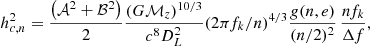
Here, e is the eccentricity of the MBHB, n is the harmonic number, and Jn(x) is the n–th Bessel function of the first kind. Also, ζ is the GW amplitude given by the combination of the redshifted chirp mass, ℳz, and the luminosity distance, DL:
Here, c is the light speed and G is the gravitational constant. The redshifted chirp mass is expressed as
with ℳ as the rest-frame chirp mass, M = m1 + m2 the total mass of the binary in the rest frame, and q = m2/m1 < 1 its mass ratio. With this definition of q, we identify m1 and m2 as the mass of the primary and secondary MBH, respectively. The variable, ι, is the inclination angle defined as the angle between the GW propagation direction and the binary orbital angular momentum,  . The quantity l(t) refers to the binary mean anomaly l(t) = l0 + 2π∫t0tfk(t′)dt′, wherefk(t′) corresponds to the observed Keplerian frequency defined as fk(t) = (1 + z)fk, r(t) with
  the rest frame Keplerian frequency and rbin(t) the semi-major axis of the MBHB orbit. In principle, rbin(t) can evolve during the observation time due to the GW emission and environmental interaction. However, here we assume that the orbital frequency and eccentricity do not evolve during the observation time, hence, fk(t) can be treated as a constant value, namely, fk (see the discussion on this assumption in Sect. 6). The orbital angular frequency is then given by ω = 2πfk, while γ is the angle that measures the direction of the pericenter with respect to the direction
  , defined as
  .
.
2.2. The timing residuals
A GW passing between the pulsar and the Earth perturbs the space-time metric, causing a modification in the arrival time of the pulse to the Earth. This induces a fractional shift in the pulsar rotational frequency,  , given by (e.g. Anholm et al. 2009; Book & Flanagan 2011)
where  is the unit direction vector to the pulsar and Δhab = hab(t, xE)−hab(tP, xP) is the difference in the metric perturbation computed at the moment in which the GW arrives at the solar system barycenter (t), and when it passed through the pulsar (tP = t − L/c, where L denotes the distance to the pulsar). We define xE to coincide with the solar system barycenter, which is the origin of the adopted coordinate system, while
  corresponds to the pulsar sky position. In practice, the PTA experiments are aimed at measuring the timing residual, which corresponds to the time-integrated effect of Eq. (6):
![$$ \begin{aligned} \begin{aligned} s(t)&= \int _{t_0}^{t} \mathrm{d}t\prime z(t\prime ) \\&= F^+(\hat{\Omega })\left[s_+(t)-s_+(t_0)\right] + F^\times (\hat{\Omega })\left[s_\times (t)-s_\times (t_0)\right]. \end{aligned} \end{aligned} $$](/articles/aa/full_html/2025/02/aa51556-24/aa51556-24-eq17.gif)
Here, s+, ×(t) = ∫t0th+, ×(t′)dt′, t0 is the time at which the observational campaign starts and t = t0 + Tobs is the epoch of the considered observation. The variable F+, × denote the ‘antenna pattern functions’ and encode the geometrical properties of the detector (for a PTA experiment the test masses are the Earth and the pulsar). In particular, F+, × depends on the GW propagation direction ( ) and the pulsar sky location (
 ). By making use of the polarisation basis tensor
  (see Taylor 2021), the pattern functions F+, × can be written as
![$$ \begin{aligned} F^+(\hat{\Omega }) = \dfrac{1}{2} \dfrac{[\hat{u}\cdot \hat{p}]^2 -[\hat{v}\cdot \hat{p}]^2}{1+\hat{\Omega }\cdot \hat{p}}, \end{aligned} $$](/articles/aa/full_html/2025/02/aa51556-24/aa51556-24-eq21.gif)
and
![$$ \begin{aligned} F^\times (\hat{\Omega }) = \dfrac{\bigl [\hat{u}\cdot \hat{p}\bigr ] [\hat{v}\cdot \hat{p}]}{1+\hat{\Omega }\cdot \hat{p}}, \end{aligned} $$](/articles/aa/full_html/2025/02/aa51556-24/aa51556-24-eq22.gif)
where  corresponds to the vector pointing to the GW source:
![$$ \begin{aligned} \hat{n} = -\hat{\Omega } = [\cos {\theta }\cos {\phi }, \, \cos {\theta }\sin {\phi }, \, \sin {\theta }], \end{aligned} $$](/articles/aa/full_html/2025/02/aa51556-24/aa51556-24-eq24.gif)
and  and
and  are defined as
![$$ \begin{aligned} \begin{aligned} \hat{u} = \frac{\hat{n}\times \hat{L}}{|\hat{n}\times \hat{L}|}&= [\cos {\psi }\sin {\theta }\cos {\phi } -\sin {\psi }\cos {\theta }, \\&\quad \cos {\psi }\sin {\theta }\sin {\phi } + \sin {\psi }\cos {\phi }, \\&\quad -\cos \psi \cos \theta ], \end{aligned} \end{aligned} $$](/articles/aa/full_html/2025/02/aa51556-24/aa51556-24-eq27.gif)
![$$ \begin{aligned} \begin{aligned} \hat{v} = \hat{u}\times \hat{n}&= [\sin {\psi }\sin {\theta }\cos {\phi } + \cos {\psi }\sin {\phi }, \\&\quad \sin {\psi }\sin {\theta }\sin {\phi } -\cos {\psi }\cos {\phi }, \\&\quad -\sin {\psi }\cos {\theta }]. \end{aligned} \end{aligned} $$](/articles/aa/full_html/2025/02/aa51556-24/aa51556-24-eq28.gif)
Here θ and ϕ are the sky location of the MBHB expressed in spherical polar coordinates (θ, ϕ) = (π/2 − Dec, RA), being Dec the declination and RA the right ascension of the binary. Finally, ψ is the polarisation angle, ranging between [0, π].
For simplicity, we considered only the Earth term1 and ignored any time evolution of the MBHB frequency, while neglecting higher order post-Newtonian effects, such as the pericenter precession and orbit-spin coupling. Those are expected to play a minor role in the output of PTA GW signal (Sesana & Vecchio 2010), and can be safely neglected, at least for a first order estimate. We will comment on the validity of these assumptions in Sect. 6. Under the framework outlined above, the values of the timing residuals can be written analytically as (Taylor et al. 2016)
![$$ \begin{aligned} \begin{aligned} s_+(t)&= \sum _{n=1}^{\infty } - \left(1+\cos ^2{i}\right) \left[\tilde{a}_n\cos {(2\gamma )} - \tilde{b}_n\sin (2\gamma )\right] \\&\quad + \left(1-\cos ^2{i}\right)\tilde{c}_n, \\ s_\times (t)&= \sum _{n=1}^{\infty } 2\cos {i} \,\left[\tilde{b}_n\cos {(2\gamma )}+\tilde{a}_n\sin {(2\gamma )} \right], \end{aligned} \end{aligned} $$](/articles/aa/full_html/2025/02/aa51556-24/aa51556-24-eq29.gif)
being:
![$$ \begin{aligned} \begin{aligned} \tilde{a}_n&= -\zeta \omega ^{-1/3}[J_{n-2}(ne)-2eJ_{n-1}(ne) (2/n)J_{n}(ne) \\&\quad + 2eJ_{n+1}(ne) -J_{n+2}(ne)]\sin (nl(t)) \\ \tilde{b}_n&= \zeta \omega ^{-1/3} \sqrt{1-e^2}[J_{n-2} (ne)-2J_{n}(ne)+J_{n+2}(ne)]\cos (nl(t))\\ \tilde{c}_n&= (2/n) \zeta \omega ^{-1/3}J_{n}(ne)\sin (nl(t)). \end{aligned} \end{aligned} $$](/articles/aa/full_html/2025/02/aa51556-24/aa51556-24-eq30.gif)
3. S/N and parameter estimations of massive black hole binaries in PTA data
In this section, we introduce the methodology used to compute the S/N and the FIM from the gravitational wave signal emitted by a single eccentric MBHB.
3.1. Signal-to-noise ratio for eccentric binaries
In general, to assess the possibility of detecting a nano-Hz CGW signal generated by an MBHB it is required to determine how its signal compares with the background noise present in the detector. This is usually done by computing the S/N. Given the deterministic nature of the CGW signal, the optimal way to compute the S/N is through matched filtering. Assuming that a CGW is present in the timing residual of a pulsar, the match filtering procedure gives the expression
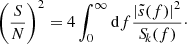
Estimating the S/N therefore requires the characterisation of the noise properties encoded in Sk(f); namely, the noise power spectral density (NPSD) of the k–th pulsar inside our array, in addition the knowledge of the signal  , which is the Fourier transforms of s(t) given by Eq. (13).
As shown by Eq. (15), the computation of the S/N requires the time residuals in the frequency domain, namely,  . However (as described in Sect. 2.1), in PTA experiments, the time residuals are framed on the time domain. Transforming these in the frequency domain can be easily addressed in the case of circular binaries given that the CGW signal is monochromatic (see e.g., Rosado et al. 2015). However, in the generic case of an eccentric binary, the signal is spread over a spectrum of harmonics and the term
  contains mixed products between residuals originated at different harmonics. To address this scenario, we worked under the assumption that the noise is a Gaussian and zero-mean stochastic stationary process and we adopted a similar approach to the one presented in Barack & Cutler (2004). In brief, even if Eq. (15) is given by the mixed product generated by different harmonics, their signal in the frequency domain is described by a delta function centred at the emission frequency, nfk. Consequently, the product of the residuals generated by harmonics emitting at different frequencies are orthogonal and cancel out. We can therefore treat each harmonic separately as a monochromatic signal and compute its S/N by exploiting the fact that
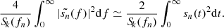
The S/N from an eccentric MBHB, for a single pulsar, is thus given by the summation in quadrature over all the harmonics:
while the total S/N in the PTA is given by the sum in quadrature of the S/N values produced in all the NPulsars included in the array:
Finally, the computation of the S/N of Eq. (17) requires a summation over all the harmonics, namely, n ∈ [1, +∞]. However the contribution to the S/N goes to zero for n → +∞ and the sum can be appropriately truncated. To select the harmonic of truncation, nmax, we adopted the simple criteria of nmax = 4 npeak, being npeak the harmonic number at which the power of the GW emission is maximised for the selected eccentricity. To compute this value we follow the numerical fit presented in Hamers (2021):
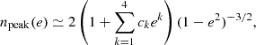
where c1 = −1.01678, c2 = 5.57372, c3 = −4.9271, c4 = 1.68506. We have checked how the exact value of nmax affects our results. Specifically, less than 1% relative difference is seen in the S/N when it is computed assuming nmax = 104 instead of nmax = 4 npeak.
3.2. Parameter estimation
Once the methodology to derive the S/N from an eccentric MBHB has been framed, the natural subsequent step is determining how well the system parameters can be measured. In the case of high S/N, they can be quickly estimated through the FIM formalism. Specifically, the GW signal we are considering is characterised by nine free parameters (see their definition in Sect. 2.1):

To reconstruct the most probable source parameters, λ, given a set of data, d, it is possible to work within the Bayesian framework and derive the posterior probability density function, p(λ|d):

where p(d|λ) is the likelihood function and p(λ) is the prior probability density of λ. If we assume that near the maximum likelihood estimated value,  , the prior probability density is flat, the posterior distribution p(λ|d) will be proportional to the likelihood and can be approximated as a multi-variate Gaussian distribution:
![$$ \begin{aligned} p(\boldsymbol{\lambda }| \boldsymbol{d}) \propto \exp \left[-\frac{1}{2}\Gamma _{ij}\Delta \lambda _i \Delta \lambda _j\right], \end{aligned} $$](/articles/aa/full_html/2025/02/aa51556-24/aa51556-24-eq42.gif)
where the indexes i and j run over all the components of the source parameter vector λ (in our case from 1 to 9), and  (
( ) are the differences between the ‘true’ source parameters (λ) and their most probable estimated values (
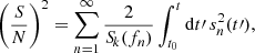
 ). Finally, Γij is the FIM, and its inverse provides a lower limit to the error covariance of unbiased estimators2. In the PTA case, the Fisher matrix is computed as
where ∂i and ∂j are the partial derivatives of time residual in the frequency domain, s(f), with respect to the λi and λj parameters, respectively. As for the S/N integral, the scalar product is defined in the frequency domain. However, we can apply the approximate identity given by Eq. (16) to write:
in which the partial derivatives are calculated numerically through
![$$ \begin{aligned} \partial _i s_n(t) = \left[\frac{s_n(t,\lambda _i + \delta \lambda _i/2) - s_n(t,\lambda _i - \delta \lambda _i/2)}{\delta \lambda _i}\right], \end{aligned} $$](/articles/aa/full_html/2025/02/aa51556-24/aa51556-24-eq48.gif)
where the step is set to be equal to δλi = 10−5λi. We note that when calculating the S/N and the FIM, we always assume to know all the parameters that fully specify the residuals, s(t).
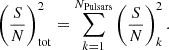
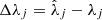
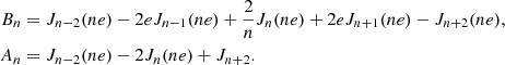
By assuming independent data streams for each pulsar in the array, the FIM obtained from the full PTA, (Γij)T, is simply given by the sum of the single FIMs derived for each pulsar, (Γij)k:
We stress that the covariance matrix is simply the inverse of the FIM (Γ−1), thus the elements on the diagonal represent the variances of the parameters ( ), while the off-diagonal terms correspond to the correlation coefficients between parameters (
 ).
).
3.3. Characterising the noise
The next fundamental ingredient in our computation is the noise description in PTA experiments. In particular, the pulsar NPSD can be broken down in two separate terms:
The term Sh(f) describes the red noise contributed at each given frequency by the sGWB generated by the incoherent superposition of all the CGWs emitted by the cosmic population of adiabatically MBHBs (Rosado et al. 2015):
For a real PTA, the noise is estimated at each resolution frequency bin of the array. In fact if we assume an observation time T, the PTA is sensitive to an array of frequency bins Δfi = [i/T, (i + 1)/T], with i = 1, …, N. If we now identify each frequency bin Δfi with its central frequency fi, then we can associate the characteristic strain produced by all the MBHBs emitting in that element with each frequency resolution element, as follows:
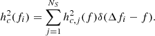
where the sum is over all sources, NS, and δ(Δfi − f) is a generalised delta function that assumes the value 1 when f ∈ Δfi, and 0 otherwise, thus selecting only MBHBs emitting within the considered bin. hc, j2(f) is the squared characteristic strain of the j–th source. Since we consider eccentric MBHBs, hc, j2(f) is the sum of the strain emitted at all the harmonics nfk, among which one has to select only those that lie within the frequency bin Δfi. Equation (29) can thus be generalised as
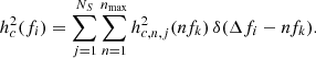
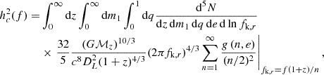
For each of the NS binaries the value of hc, n2, is given by Amaro-Seoane et al. (2010):
where 𝒜 = 1 + cos(i)2, ℬ = −2cos(i) and Δf = 1/T is the frequency bin width. The value of g(n, e) is computed according to
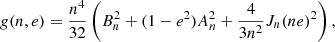
where An and Bn are
We stress that when evaluating the detectability of a given MBHB we will not take into account the contribution of its hc, j2(f) when computing the value of Sh(f).
We stress that an eccentric population of MBHBs could produce an sGWB with time-dependent features, leading to the breakdown of the stationarity assumption which we rely on (see Eq. 28). In this context, Falxa et al. (2024) recently developed a perturbative approach for identifying non-stationary features in the sGWB, showing that a near-eccentric source could introduce a time-dependence behavior in the recovery of the background parameters (amplitude and slope). Despite these recent efforts, the level of non-stationarity in the sGWB generated by an entire population of eccentric MBHBs remains unclear. Future studies are crucial for developing new frameworks able to address correlations between noise at different frequency bins. Since the treatment of non-stationary features goes beyond the scope of this paper we will assume throughout this work that all noise sources are stationary.
The term Sp(f) in the NSPD encodes all sources of noise unrelated to the sGWB, which are related to the telescope sensitivity, intrinsic noise in the pulsar emission mechanism, pulse propagation effects and so on. PTA collaborations parameterise the pulsar noise as a combination of three different terms:

Sw accounts for processes that generate a white stochastic error in the measurement of a pulsar arrival time. These include pulse jitter, changes in the pulse profile with time, or instrumental artefacts. Such processes are uncorrelated in time and the resulting noise is modelled as Sw = 2Δtcadσw2, where it is commonly assumed that the pulse irregularity is a random Gaussian process described by the root mean square value σw. Here, Δtcad is the time elapsed between two consecutive observations of the same pulsar, namely, the observation cadence. Then, Sred(f) and SDM(f) describe the achromatic and chromatic red noise contributions, respectively. While the former is the result of the pulsar intrinsic noise, the latter is the result of spatial variations in the interstellar electron content along the line of sight between the observer and the pulsar. These two red noises are usually modeled as a stationary stochastic process, described as a power law and fully characterised by an amplitude and a spectral index. Given the several mitigation strategies that can be employed for taking into account DM noise, in our analysis we ignored its contribution to the pulsar noise budget.
4. Massive black hole binary populations and pulsar timing arrays
4.1. The population of binaries
In this section, we briefly present the procedure used to generate the different populations of eccentric MBHBs that will be used throughout this paper. For further details, we refer to Sesana (2010, 2013b) and EPTA Collaboration and InPTA Collaboration (2024a).
4.1.1. Model description
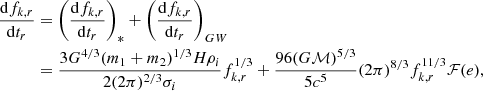
To study the detectability of single MBHBs, it is necessary to characterise their cosmological population as a whole. The sGWB spectrum generated by such a population can be calculated as the integrated emission of all the CGW signals emitted by individual binaries. Thus, the inclination and polarisation average3 characteristic strain of the sGWB can be expressed as
where d5N/(dm1 dq dz de dtr) is the comoving number of binaries emitting in a given logarithmic frequency interval, dlnfk, r, and primary mass, mass ratio, eccentricity and redshift in the range [m1, m1 + δm1], [q, q + δq], [e, e + δe] and [z, z + δz], respectively. In particular, this quantity can be re-written as
![$$ \begin{aligned} \begin{aligned} \frac{\mathrm{d}^5 N}{\mathrm{d}z\, \mathrm{d} m_1\, \mathrm{d}q\, \mathrm{d}e\, \mathrm{d} \ln f_{\mathrm{k} ,r}}&= \frac{d^3n}{\mathrm{d}z\, \mathrm{d} m_1\, \mathrm{d}q} \left(\frac{1}{f_{\mathrm{k} ,r}}\frac{\mathrm{d}f_{\mathrm{k} ,r}}{\mathrm{d}t_r}\right)^{-1} \left[\frac{\mathrm{d}z}{\mathrm{d} t_r} \frac{\mathrm{d} V}{\mathrm{d}z}\right] \\&= \frac{d^3n}{\mathrm{d}z\, \mathrm{d} m_1\, \mathrm{d}q} \left(\frac{1}{f_{\mathrm{k} ,r}}\frac{\mathrm{d}f_{\mathrm{k} ,r}}{\mathrm{d}t_r}\right)^{-1} \; \frac{4\pi c D_L^2}{(1+z)}, \end{aligned} \end{aligned} $$](/articles/aa/full_html/2025/02/aa51556-24/aa51556-24-eq61.gif)
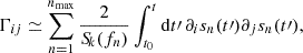
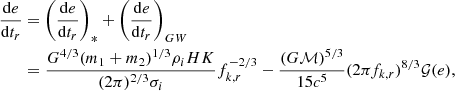
where n = dN/dV, d3n/(dz dm1 dq) is the differential merger rate comoving density of MBHBs and fk, r(dtr/dfk, r) represents the binary evolution timescale, which implicitly takes into account the variation of the hardening rate with the binary eccentricity (i.e. at fixed orbital frequency, eccentric binaries evolve faster). Following Sesana (2013b), the merger rate of MBHs can be expressed in terms of the galaxy merger rate, (d3nG/(dz dM* dq*), as
![$$ \begin{aligned} \begin{aligned} \frac{d^3n}{\mathrm{d}z\, \mathrm{d} m_{1}\, \mathrm{d}q}&= \frac{\mathrm{d}^3n_{\rm G}}{\mathrm{d}z\, \mathrm{d} M_{*}\, \mathrm{d}q_{*}} \frac{\mathrm{d} M_*}{\mathrm{d} m_{1}} \frac{\mathrm{d}q_*}{\mathrm{d} q}\\&=\left[\frac{\phi (M_*,z)}{M_* \ln 10} \frac{\mathcal{F} (z,M_*,q_{*})}{\tau (z,M_*,q_{*})} \frac{\mathrm{d}t}{\mathrm{d}z}\right] \frac{\mathrm{d} M_*}{\mathrm{d} m_{1}} \frac{\mathrm{d}q_*}{\mathrm{d}q}, \end{aligned} \end{aligned} $$](/articles/aa/full_html/2025/02/aa51556-24/aa51556-24-eq62.gif)
where ϕ(M*, z) is the galaxy stellar mass function and ℱ(z, M*, q*) the differential fraction of galaxies with mass M* at a given redshift paired with a satellite galaxy of mass in the interval [q*M*, (q* + dq*)M*]4. The value τ(z, M*, q) is deduced from N-body simulations and corresponds to the typical merger timescale for a galaxy pair with a given mass, redshift and mass ratio. The term (dM*/dm1)(dq*/dq) associates an MBH with each galaxy in the pair by using the MBH galaxy bulge mass scaling relation:

where ℰ represents an intrinsic scatter, generally around 0.3 − 0.5 dex (Sesana et al. 2016), and α and β define the zero point and logarithmic slope of the relation, respectively. To transform the total stellar mass into bulge mass, the relation M* = fb MBulge described in Sesana et al. (2016) is assumed.
Finally, the hardening of the binary in Eq. (36) is determined by using the stellar models of Sesana (2010):
and
where
and σi and ρi are the velocity dispersion and stellar density at the binary influence radius. H and K represent the hardening rate and the eccentricity growth rate, calibrated against numerical three-body scattering experiments (Sesana et al. 2006).
4.1.2. Generating MBHB populations consistent with PTA measurements
As described above, the cosmological coalescence rate of MBHBs depends on different assumptions about the galaxy merger rate and correlations between MBHBs and their hosts. In particular, the library of models presented in Sesana (2013b), Rosado et al. (2015), Sesana et al. (2016) combines a number of prescriptions from the literature which we summarise here:
-
Galaxy stellar mass function. Five different observational results are taken from the literature (Borch et al. 2006; Drory et al. 2009; Ilbert et al. 2010; Muzzin et al. 2013; Tomczak et al. 2014) and matched with the local mass function (Bell et al. 2003). For each of these functions, upper and lower limits were added to account for the errors given by the authors best-fit parameters. On top of this, an additional 0.1 dex systematic error was included to consider the uncertainties in the stellar masses determination. For all the mass functions, we separate between early/late-type galaxies and the analysis was restricted to z < 1.3 and M* > 1010 M⊙, since we expect that these systems contribute the most to the sGWB signal (see e.g. Sesana et al. 2009; Kelley et al. 2018; Izquierdo-Villalba et al. 2023).
-
Differential fraction of paired galaxies. The observational results of Bundy et al. (2009), de Ravel et al. (2009), López-Sanjuan et al. (2012) and Xu et al. (2012) were used when accounting for the evolution of the galaxy pair fraction.
-
Merger timescale for a galaxy pairs. We follow the fits done from the N-body and hydrodynamical simulations of Kitzbichler & White (2008) and Lotz et al. (2010).
-
Galaxy-MBH scaling relation. The masses assigned to each merging galaxy pair were drawn from several observational relations. However, given the high normalisation of the observed PTA signal, we only considered relations presented by Kormendy & Ho (2013), McConnell & Ma (2013) and Graham & Scott (2013).
To save computation time, we performed an ad hoc down-selection of the models and limited our investigation to 108 combinations of the above prescriptions producing a distribution of sGWB amplitudes consistent with the measured PTA signal, as per Fig. 2 of EPTA Collaboration and InPTA Collaboration (2024a).
As for the environmental coupling and eccentricity evolution, we adopted the following prescriptions:
-
Stellar density profile. Following Sesana (2010), the stellar density profile is assumed to be a broken power law following an isothermal sphere outside the influence radius, ri = 1.2 pc (M/106 M⊙)0.5, and a profile
at r < ri. Here, ρi = σ2/(2πGri2) and σ is determined from the Tremaine et al. (2002) scaling relation (see Sesana 2010, for further details). C is a normalisation factor of the stellar density profile and is assumed to take three different values (0.1, 1 and 10), to investigate the effect of changing the typical density of the environment.
-
Initial eccentricity. During the tracking of the hardening evolution, all the binaries are assumed to start with an initial eccentricity e0 at binary formation. Throughout the paper, we consider ten initial values of e0 = 0, 0.1, 0.2, 0.3, 0.4, 0.5, 0.6, 0.7, 0.8, 0.9.
Using the 108 population model, 10 eccentricity values, and 3 environment normalisations defined above, we generated 3240 numerical distributions of MBHBs using Eq. (36) and for each distribution, we performed a ten Monte Carlo sampling for a grand total of 32 400 MBHB populations. Each population consists of a list of ≈105 binaries characterised by their chirp mass, redshift, orbital frequency, and eccentricity. Due to the computational cost required to compute the FIM, the latter has been calculated only for a subsample of 3240 populations (10% of the total).
4.2. The array of pulsars
We explore the feasibility of detecting CGW signals using two different pulsar timing arrays: MeerKAT (NPulsars = 78) and SKA (NPulsars = 200). While pulsar monitoring at MeerKAT has been ongoing for 4.5 years, it will be superseded by the SKA Mid array by 2027. Given these constraints, we chose 10 years for MeerKAT while the 30-year time span of SKA follows projections commonly used in the literature.
(i) MeerKAT is a 64-antenna radio interferometer telescope located in South Africa. The regular monitoring of millisecond pulsar timing by MeerKAT is the basis of the MPTA. Recently, it was released the initial 2.5-years MPTA data (Miles et al. 2023). While the current data includes 88 pulsars, the release only contains the 78 pulsars that have at least 30 observations over this observing span, with a typical cadence of 14 days. The upper panel of Fig. 1 shows the position of those pulsars in the sky. Table A.1 of Miles et al. (2023) also reported the noise properties of each of the 78 pulsars, accounting for white-noise terms, frequency-dependent DM variations, and an achromatic red-noise process (see Sect. 3.3). In this work, we will use a 10-year MPTA-like system, featuring the same set of pulsars (number, sky position, and noise model) as the one presented in Miles et al. (2023).
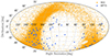 |
Fig. 1. Sky position of the pulsars included in the PTA experiments used in this work. The pulsars from MPTA are displayed in blue whereas the ones of SKA (full PsrPopPY population) are depicted in orange. |
(ii) Square Kilometer Array Mid telescope (SKA, Dewdney et al. 2009) planned to be operative in 2027, will be a large radio interferometer telescope whose sensitivity and survey speed will be an order of magnitude greater than any current radio telescope. For this work, we simulate a 30-year SKA PTA with 200 pulsars featuring a white noise of σw = 100 ns and an observing cadence of 14 days. To picture a more realistic scenario we also include red noise to the total noise power spectral density in Eq. (34), parameterised as a power law (see e.g. Lentati et al. 2015) of the form
where Ared the amplitude at one year and γred the spectral index. Red noise properties are drawn to be consistent with those measured in the EPTA DR2Full using the following procedure. We fit a linear log Ared − γ relation to the measured red noises in Table 4 of EPTA Collaboration and InPTA Collaboration (2023b). We then assign Ared and γ parameters consistent with this relation to 30% of the pulsars in the SKA array, drawing Ared randomly from a uniform log-distribution in the range to −15 < log Ared < −14, for which the corresponding γ is > 3. In this way, we mimic in the SKA array the fraction and properties of EPTA DR2Full pulsars with a robust red noise contribution. Note that while the remaining 70% of the pulsars will likely display some lower level of red noise, this is unlikely to affect the properties of the detected CGWs. In fact, for those pulsars the main stochastic red noise component is going to be the sGWB itself, which is already included in our calculation.
We then employ the pulsar population synthesis code PsrPopPY5 (Bates et al. 2014) to draw a realistic distribution of pulsars in the array. PsrPopPY generates and evolves realistic pulsar populations drawn from physically motivated models of stellar evolution and calibrated against observational constraints on pulse periods, luminosities, and spatial distributions. The final population of pulsars (105) is selected such that they would be observable (S/N > 9) by a SKA survey with an antenna gain of 140 K/Jy and integration time of 35 minutes. To avoid a particularly (un)fortunate pulsar sky disposition, from this distribution, we selected a different set of 200 pulsars for each one of the MBHB population presented in Sect. 4.1. The sky distribution of the whole pulsar sample of SKA is presented Fig. 1. Since PsrPopPy simulates hyper-realistic distributions of pulsars generated using theoretical considerations and observational constraints, the bulk of the generated full population of pulsars will lie close to the Galactic plane. However, the exceptional sensitivity of the SKA would also allow us to choose the most isotropic distributions of pulsars in the PTA, maximising sensitivity to any GW signals searched for by the PTA.
Figure 2 presents the sensitivity curve of our SKA PTA and MPTA computed using HASASIA Python package (Hazboun et al. 2019). As expected, SKA PTA features better sensitivity than the MPTA. However, at low frequencies, both of them are limited by the sGWB. To guide the reader, Fig. 2 also displays the sensitivity curves of SKA and MeerKAT PTAs when only white noise is considered. As shown in Fig. 2, for MPTA the two sensitivity curves are almost identical since only 4 of the 78 pulsars listed in Miles et al. (2023) have a reported red noise. Conversely, when achromatic red noise is included in the SKA PTA, due to the larger fraction of pulsars affected by it, the red noise slightly hider the array’s sensitivity at the lowest frequencies (< 10−8 Hz).
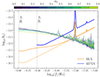 |
Fig. 2. Sensitivity curves of 10-year MPTA (blue) and 30-year SKA (orange) computed from HASASIA. The vertical dashed lines correspond to the frequency associated with the observing time span of MPTA and SKA (highlighted with vertical dashed lines). For completeness, the square mean of sGWB produced by our MBHB populations at different e0 models are represented in different colors. Pale (dark) blue and orange lines correspond to the MPTA and SKA sensitivity curves when accounting for pulsar white noise only (white plus red noise). |
4.3. Identifying individually resolvable MBHB
To extract individually resolvable CGWs, we employ a recursive technique similar to Karnesis et al. (2021) and Pozzoli et al. (2023). We sort the MBHB population by strain amplitude according to the expression in Eq. (31), but selecting only the second harmonic (n = 2). Following this ranking, we calculate the S/N of each source according to Eq. (18), including in the sGWB contribution to the noise the signals produced by all the other MBHBs. Whenever one source exceeds the S/N > 5 for SKA or S/N > 3 for MPTA6, the source is deemed resolved and its contribution to the sGWB is subtracted. As a consequence, the level of the noise in the pulsar array is lowered as well (see Eq. (28)), making more feasible the detection of dimmer CGWs that might be otherwise unobservable. We therefore re-evaluate the detectability of all the remaining sources by making use of the new (lowered) background. This procedure is repeated until there are no resolvable sources left in the analyzed MBHB population.
The above recursive procedure must be applied to several thousands of MBHB populations, each including ∼105 systems, which becomes extremely time-consuming. To boost the efficiency of our pipeline, we established a criterion that allows us to select only those sources with the largest chance of being resolvable. We established a threshold in the value of h = 2ζG5/3(πfk)2/3/c4 (hereafter hth) below which we do not compute the S/N, deeming the source too dim to be resolved. To determine the exact value of the threshold, we have computed the number of resolvable sources (Nres) at different hth cuts for 96 randomly selected MBHB catalogs at three different values of e0. We imposed the condition S/N > 5 for CGW detection and computed the number of resolvable sources using the SKA PTA, because of its larger performance in resolving dim GW sources compared to MPTA. Since, for this analysis, we are interested in the dimmest MBHB that the PTA experiment can resolve, we conservatively consider SKA PTA which features only white noise. Figure 3 shows the median number of Nres as a function of hth. As expected, Nres increases towards small values of hth, but it saturates below a certain threshold. This behavior is seen for all e0 used to start the MBHB evolution. Taking into account Fig. 3, throughout this work we will use the conservative value of hth = 6 × 10⁻¹⁷. We stress that small fluctuations are seen in the Nres median below our fiducial threshold. However, they are not statistically significant (±1 source) and the selected hth provides a good compromise between accuracy and computational efficiency. The recursive S/N evaluation-subtraction procedure is thus performed only on the subset of binaries with h > hth, providing a considerable speedup of the calculation.
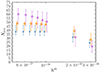 |
Fig. 3. Median number of resolvable sources of 96 randomly selected catalogs (Nres), with three diffented initial eccentricity, e0 = 0.0, e0 = 0.5, e0 = 0.9, as a function of the adopted thresholds in the GW signal amplitude (hth). Each set of marks and colors represents populations with different e0, as labeled in the figure. The values of Nres are computed by using the SKA PTA. |
5. Results
In this section, we present the main results of our work. The analysis has been performed taking into account different values of e0. This has enabled us to characterise the effect of eccentricity in determining the number of resolvable sources and the accuracy of the parameter estimation from the detected signal. To avoid confusion with the initial eccentricity used in the hardening model, e0, throughout the whole section we will tag the eccentricity of the detected MBHB as ers.
5.1. Number of resolvable sources
The upper panel of Fig. 4 shows the median number of resolvable sources (Nres) detected by the SKA and MPTA. The results have been divided according to the eccentricity at which the MBHB population was initialised (e0). This classification allows us to understand the impact of the eccentricity of the global MBHB population on the prospects of CGW detection. The median number of resolvable sources for 10-year MPTA is 4, independently of e0. Conversely, 30-years SKA provides larger Nres values (∼35), increasing with eccentricity. In particular, the number of detected binaries starts to increase when e0 > 0.2.
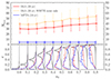 |
Fig. 4. Number of resolvable sources (Nres) for as a function of e0. Open dots represent median values from all the considered MBHB population models, while error bars represent the 84 and 16 percentile of the distribution. Blue points correspond to the results of 10-year MPTA data with S/N > 3, while the red ones represent the predictions for 30-year SKA data with S/N > 5. Orange points represent the 30-year SKA results but when accounting only for the white pulsar noise. The lower panel shows the eccentricity distribution of the whole MBHB population for different e0 models (black) and the eccentricity distribution of the MBHBs detectable as CGW sources (ers) for SKA PTA (red) and for MPTA (blue). We note that all the distributions are normalised to the same peak value for visualisation purposes. |
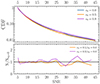 |
Fig. 5. Cumulative distribution function (CDF) of the S/N featured by MBHBs detected by 30-year SKA PTA. Blue, orange, and purple curves represent the CDF of all the models generated with e0 = 0, 0.5 and 0.9, respectively. The lower panel presents the number of sources found with a given value of S/N for e0 = 0.5 and e0 = 0.9 models (orange and purple line) normalised with the same value found in the e0 = 0 case. |
This trend can be ascribed to the appearance of resolvable high-eccentric MBHBs, with an observed Keplerian frequency outside of the PTA frequency range. Given their large eccentricity, these systems can push a large fraction of their GW signal inside the PTA band (more details in the description of Figs. 6 and 7 below). The eccentricity distribution of the detected MBHBs is presented in the lower panel of Fig. 4. Regardless of the adopted array, the eccentricity distribution of resolved sources peaks at lower values compared to the underlying overall MBHB population. Therefore, the eccentricity of the detected systems is not a good tracer of the eccentricity of the global MBHB population. This is because the more massive binaries, which circularise faster (see Eq. 40), are also more likely to be detected. Compared to MPTA, it is clear that the SKA PTA can generally observe more eccentric MBHBs, which is expected due to its longer timespan. In fact, the SKA PTA sensitivity extends to lower frequencies, where MBHBs had less time to circularise due to GW emission. For completeness, Fig. 4 depicts the number of resolvable sources for SKA PTA when only the pulsar white noise is taken into account. As shown, when the red noise is neglected the number of resolvable sources increases by ∼30%.
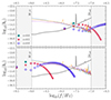 |
Fig. 6. Characteristic strain (hc) as a function of observed frequency (f). The upper panel shows a binary with ℳ ∼ 108.5 M⊙ and the observed Keplerian frequency fk ∼ 10−8 Hz; while the lower panel shows a binary of ℳ ∼ 1010 M⊙ and fk ∼ 10−9.5 Hz outside the SKA PTA sensitivity curve. In each panel, blue, orange, and purple lines represent the root mean square of the sGWB generated by all the models with e0 = 0, 0.5 and 0.9, respectively. The black line corresponds to the sensitivity curve of SKA PTA (white and red noise) 30-year data. The colored dots represent how the signal of an MBHB is distributed across different frequencies when the eccentricity is varied between 0, 0.5 and 0.9. |
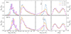 |
Fig. 7. Chirp mass distribution (ℳ, upper left panel), redshift (z, upper right panel), twice the observed Keplerian frequency (f2, lower left panel), and inclination angle (i, lower right panel) of the detected MBHBs. Each color represents the distributions when different eccentricity values are used to evolve the MBHB population (e0 = 0, blue, e0 = 0.5, orange and e0 = 0.9 purple). NBin represents the number of objects in a given bin of the histogram while Ntot is the total number of objects analyzed. While the upper panels represent the results for 30-year SKA PTA, the lower ones correspond to 10-year MPTA. |
Finally, Fig. 5 shows the distribution of the S/Ns of resolvable sources. For clarity, we only presented the results for the SKA PTA given that MPTA features the same trends (but extended down to S/N = 3). As we can see, 90% of the detected systems present S/N < 15, but there is a large tail towards larger values. Despite being just a few, the remaining 10% of sources with S/N > 15 will be optimal targets for multimessenger astronomy, since their sky localisation will be small enough to perform electromagnetic follow-ups (see Sect. 3.2 and Goldstein et al. 2019). Finally, to compare the S/N distributions for models initialised with different eccentricities we compute the ratio between the number of sources at different S/N bins for e0 = 0.5, 0.9 by the detected population with e0 = 0.0. As can be seen, no major differences in the S/N distribution are found.
5.2. Properties of the resolvable sources
In this section, we study the properties of the resolvable sources and explore possible dependencies with the eccentricity of the underlying MBHB population. For the sake of clarity, the analysis has been done only using three reference eccentricity models: e0 = 0.0, 0.5 and 0.9.
The left panels of Fig. 7 present the chirp mass distribution of the MBHB population detected by SKA and MPTA experiments. As shown, both PTAs will detect MBHBs with ℳ ∼ 109.5 M⊙, although MPTA will be biased towards more massive systems given its lower sensitivity. Interestingly, the detection of ℳ ≲ 109 M⊙ binaries by SKA is preferred when the underlying MBHB population is initialised with low eccentricities (e0 < 0.5). This is due to the typical eccentricity and observed Keplerian frequency of ℳ < 109 M⊙ systems. These MBHBs are placed at fk ∼ 10−8.5 Hz independently of e0, but their eccentricity raises when e0 increases (e.g. ∼0.4 and ∼0.6 for e0 = 0.5, 0.9 models, respectively). These relatively high values of fk and eccentricity cause these systems to emit part of their GW strain at high frequencies where the PTA sensitivity is already degrading. The net effect is the decrease of the source S/N with respect to a non-eccentric case. To illustrate this, the top panel of Fig. 6 presents the characteristic GW strain versus observed GW frequency for three binaries with the same mass and Keplerian frequency but different eccentricities. As shown, for circular binaries all the emitted power falls in the frequency region in which the PTA has the best sensitivity. However, for the extreme case of e > 0.5 most of the power is pushed at f > 3 × 10⁻⁸ Hz where the PTA is less sensitive. Consequently, our analysis suggests that the detection of low-mass MBHBs (ℳ < 109 M⊙) will be hindered in highly eccentric populations.
The redshift distribution of the resolvable sources is presented in the middle-left panels of Fig. 7. The distribution peaks at z < 0.25, independently of the PTA experiment used and the eccentricity of the underlying MBHB population. The SKA resolved population has a longer tail at high redshifts, due to its better sensitivity. Moreover, there is a small trend towards higher redshifts with increasing eccentricity, more prominent in SKA than MPTA. The frequency distribution of the second harmonic (i.e. the GW emission frequency of circular binaries) of the resolved binaries is shown in the middle-right panels of Fig. 7. The peak of the distribution seats around ∼10−8.5 − 10−8 Hz, being systematically higher for SKA PTA given its better sensitivity at high frequencies. As anticipated in Sect. 5.1, models with eccentric binaries enable the detection of MBHBs whose f2 = 2fk is smaller than the minimum frequency allowed by the PTA observing time. In the extreme case of e0 = 0.9, up to half of the detected systems display this feature in the MPTA array. An illustrative example of how the strain is distributed among all the harmonics for a source with Keplerian frequency outside the PTA band can be seen in the lower panel of Fig. 6. Finally, the inclination distribution shown in the rightmost panels of Fig. 7 is bimodal, preferring face-on/face-off binaries with respect to the observer (i < 50 deg and i > 125 deg). This is simply due to the angular pattern emission of GWs, which are stronger along the binary orbital angular momentum axis.
5.3. MBHB parameter estimation
Here, we explore the precision to which the CGW source parameters can be determined. To this end, we make use of the procedure presented in Sect. 3.2. We focus on parameters of astrophysical relevance. Specifically, the GW amplitude, ζ, the observed Keplerian frequency, fk, the orbital eccentricity, ers, the inclination angle, ι, and the initial orbital phase, l0. The latter parameters might help the identification of distinctive electromagnetic counterparts. In fact, accreting binaries at low inclination angles might appear as Type I AGN, displayng considerable variability in the optical/UV, while relativistic jets could be observable for nearly face-on systems (e.g. Fedrigo et al. 2024; Gutiérrez et al. 2024). Moreover, precise phase determination of eccentric binaries allows us to clearly identify the periastron passage epochs, which can be associated with a dimming in the electromagnetic emission due to temporary mini-disc disruptions caused by the close flyby of the two MBHs (Cocchiararo et al. 2024). Finally, we combine the two angles defining the source position in the sky to determine the 2D sky localisation uncertainty as (Sesana & Vecchio 2010)
where σθ, ϕ is the correlation coefficient between θ and ϕ computed from the Fisher matrix. With this definition the probability of a GW source to be found outside a certain solid angle ΔΩ0 is proportional to e−ΔΩ0/ΔΩ. Consequently, ΔΩ is an important quantity to take into account given that it provides information about the accuracy of pinpointing the GW source in the sky. Moreover, its specific value will shed light on the possibility of carrying out multimessenger studies by placing constraints on the size of the area to scan for electromagnetic follow-ups (see, e.g. Lops et al. 2023; Petrov et al. 2024).
Our results are presented in Fig. 8 for the SKA PTA as a function of the eccentricity of the detected source, ers, to determine its potential impact on the parameter estimation. MPTA parameter estimation features the same trends and is shown in Appendix A. Since the estimation precision depends on the source S/N, we have performed this exploration at fixed bins of S/N: 5 < S/N < 10, 10 < S/N < 15, and S/N > 15. For each case, we show the median value on the error of the parameter recovery and the central 68% of the distribution. The recovery of the GW amplitude displays a small correlation with ers, slightly improving for high eccentric binaries. For instance, the median relative error for systems with S/N > 15 and ers < 0.1 is ∼30% while for high eccentric cases is reduced down to ∼20%. As it is the case for all parameters, the GW amplitude recovery precision scales linearly with the inverse of the S/N. Notably, while at S/N > 15 the source amplitude can be determined with a median relative error of 0.2−0.3, at S/N < 10 it is poorly constrained. Conversely, the Keplerian frequency is extremely well determined, with a relative error that is always smaller than 1%. In this case, the trend with eccentricity is reversed, with the median error increasing with ers.
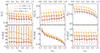 |
Fig. 8. Accuracy in recovering the source parameters as a function of the eccentricity of the detected source, ers: GW amplitude (Δζ/ζ, top left), Keplerian frequency (Δfk/fk, top middle), eccentricity (Δers, top right), inclination angle (Δι, bottom left), the initial phase of the orbit (Δl0, bottom middle) and sky localisation (ΔΩ, bottom right). All the results have been divided into three different S/N bins 3 < S/N < 10 (orange), 10 < S/N < 15 (dark orange), and S/N > 15 (dark red). |
The error associated with the binary eccentricity improves for highly eccentric systems, with values as low as ∼1 − 5% at ers > 0.6. The inclination of the MBHB orbit is essentially unconstrained, especially for systems at small S/N and for small eccentricities. The poor estimation of the inclination angle is likely due to its degeneracy with the GW amplitude, ζ; for the same reason, this can only be weakly constrained, with a relative error of around 30% at best. Further details can be found in the appendix. The initial phase of the orbit displays a clear dependence on ers, given it is better constrained for large eccentric cases. For instance, at 10 < S/N < 15, the Δl0 value associated with ers < 0.2 MBHB is ∼10 deg, while it drops down to ∼1 deg for ers > 0.6. This is not surprising since, for an eccentric orbit, the GW emission is strongly localised close to the pericenter; this allows for a precise measurement to be obtained for the orbital phase of the system.
Finally, the lower right panel of Fig. 8 presents the sky localisation. Interestingly, it does not show any dependence with ers; however, as expected, it strongly improves with S/N, since the parameter is characterised by a theoretical scaling with S/N−2. Binaries detected at 5 < S/N < 10 have a median sky-localisation of ΔΩ ∼ 200 deg2, making multimessenger follow-ups extremely challenging. On the other hand, systems with S/N > 15 feature median ΔΩ ∼ 20 deg2. We note that the 68% confidence region extends down to ≈2 deg2. Since SKA can resolve 30−40 binaries and about 10% of them will have S/N > 15 (see Fig. 5), we can therefore expect at least one CGW with source localisation at the ∼deg2 level, which would be a perfect target for electromagnetic follow-ups.
6. Caveats
In this section, we discuss the main caveats and assumptions related to the methodology.
6.1. Time-evolving binaries
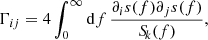
We have assumed that the MBHB orbital frequency does not evolve during the PTA observation time. However, this simplification may not hold, especially for massive and high-frequency binaries given their shorter GW timescales (see Eq. 39). To explore the fraction of MBHBs in our catalogues in which the non-evolving assumption is not fulfilled, we have computed the following quantity:
![$$ \begin{aligned} \mathcal{D} _f = \frac{\left[\frac{\mathrm{d}f_k}{\mathrm{d}t} T_{\rm obs}\right]}{\Delta f}\cdot \end{aligned} $$](/articles/aa/full_html/2025/02/aa51556-24/aa51556-24-eq70.gif)
Here, dfk/dt is determined according to Eq. (39); however, for simplicity, we accounted only for the GW term, while the factor (dfk/dt)×Tobs corresponds to the variation of the observed Keplerian frequency over the PTA observational time. The division by Δf accounts for the total variation of the MBHB frequency within the frequency bin width given by the PTA observation span. The upper panel of Fig. 9 presents the distribution of 𝒟f for all the binaries in our catalogue with h > hth (see Sect. 4.3). As shown, the distribution peaks at low values of 𝒟f (∼10−6), implying an almost null evolution of the binary frequency. Nevertheless, some cases show 𝒟f > 1, but they correspond to less than 0.1% of the MBHB population. The lower panel of Fig. 9 presents the 𝒟f distribution only for the subset of sources that are resolvable by SKA PTA. Not surprisingly, the distribution for this sub-sample of binaries peaks at larger values. This shift is caused by the fact that individually resolvable MBHBs are intrinsically systems with large masses and high frequencies (see Fig. 7). Despite this, the bulk of the system feature 𝒟f ∼ 10−3, consistent again with non-evolving binaries. Also for this sub-sample, binaries with 𝒟f > 1 only account for 0.1% of the resolvable sources. In light of these results, we can conclude that our assumption of non-evolving binaries can be safely adopted.
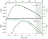 |
Fig. 9. Probability distribution function (PDF) of 𝒟f for binaries featuring h > hth (top panel) and binaries detected by SKA PTA (S/N > 5, bottom panel). In both panels, green lines correspond to the cumulative distribution function (CDF). |
6.2. Pericenter precession
Another assumption that is relevant to discuss concerns the inclusion of the pericenter precession. To quantify its impact on the S/N recovery, we adopted the same criteria presented in Sesana & Vecchio (2010). The precession of the pericenter induces an additional shift in the observed Keplerian frequency given by  with
with
This causes a bias in the recovery of the orbital frequency. However, this effect can be neglected as long as the shift caused by pericenter precession over the observed time is small compared to the frequency resolution of the detector, Δf. This is equivalent to enforce the condition 𝒟γ ≪ 1, where
![$$ \begin{aligned} \mathcal{D} _\gamma = \frac{\left[\frac{\mathrm{d}^2\gamma }{\mathrm{d}t^2} T_{\rm obs}\right]}{\Delta f}, \end{aligned} $$](/articles/aa/full_html/2025/02/aa51556-24/aa51556-24-eq73.gif)
with
![$$ \begin{aligned} \dfrac{\mathrm{d}^2\gamma }{\mathrm{d}t^2} = \dfrac{96 (2\pi )^{13/3}}{(1-e^2)c^7} [(1+z)M]^{2/3}\mathcal{M} _z^{5/3}G^{7/3}f_k^{13/3}. \end{aligned} $$](/articles/aa/full_html/2025/02/aa51556-24/aa51556-24-eq74.gif)
Fig. 10 shows the distribution of 𝒟γ for all MBHBs with h > hth (top panel) and for those detected by the SKA PTA (lower panel). Similar to the 𝒟f result, the systems with 𝒟γ > 1 represent only 0.1% of the resolved MBHBs. As a consequence, the effect of the pericenter precession can be ignored for our astrophysical-motivated populations of MBHBs.
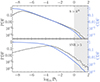 |
Fig. 10. Probability distribution function (PDF) of 𝒟γ for binaries featuring h > hth (top panel) and binaries detected by SKA PTA (S/N > 5, bottom panel). In both panels, blue lines correspond to the cumulative distribution function (CDF). |
6.3. Pulsar term
Similarly to other works, we did not account for the pulsar term since its inclusion in the matched filtering methodology requires a precise estimate of the distance between the pulsar and the Earth. To date, only a very reduced sample of pulsars has such an accurate measurement of this quantity. Despite this, ongoing efforts are being made to calculate the pulsar distance via the measurement of pulsar spin down and annual parallax motion (see e.g. Reardon et al. 2016).
When it comes to 2D sky localisation, including the Pulsar term in the analysis does not appear to make a significant difference in the size of the localisation area, at least in the case of circular, GW-driven binaries. It can, however, cause a small bias compared to the true sky location (Ferranti et al. 2024). Therefore, while Earth term-only estimates are robust in terms of localisation precision, including the pulsar term in the analysis might be required to pinpoint the correct direction in the sky.
Including the pulsar term in the CGW searches could also provide key information on how the MBHB evolves during the times needed for the pulse to cover the Earth-Pulsar distance. Under the assumption of GW-driven binaries, identification of the pulsar term allows us to effectively separate the system chirp mass from the distance in the signal amplitude parameter ζ (Ferranti et al. 2024 for examples involving circular binaries), greatly improving 3D localisation of the source in the sky. This assumption, however, is not necessarily fulfilled. At the low frequencies probed by PTAs, MBHBs can be still coupled to their environment, especially at the time of Pulsar-term production. In fact, since the typical Earth-Pulsar separation can range up to thousands of light years, the Pulsar and Earth terms of the signal could inform us about the binary properties at two different evolutionary stages. In this case, the change of parameters such as the orbital frequency and the eccentricity could help to better understand the environment in which the MBHB resided. As shown in Eq. (39), the Keplerian frequency of a binary evolving only due to GW emission varies as ∝f11/3, while if its dynamics is ruled by stellar scattering events, it changes as ∝f1/3. Including environmental coupling, however, increases the number of parameters in the model, and whether GW and environmental effects can be efficiently separated in a real analysis has still to be investigated.
6.4. Further complications in source detectability
Throughout this work, we use a simple S/N criterion to define source detectability, regardless of the nature of the GW signal. However, the shape of the waveform can be significantly different for circular and highly eccentric binaries and while the detectability of the former has been extensively demonstrated in the literature (Babak & Sesana 2012; Ellis et al. 2012; Ellis 2013), much less has been done on the eccentric binary front (Taylor et al. 2016). This is especially true for sources with f2 < 1/T, which can constitute up to 50% of the resolvable CGWs in the limit of high eccentricities for the MPTA (see Fig. 7). For these systems, the waveform consists of a single burst-like spike coincident with the binary periastron passage (e.g. Amaro-Seoane et al. 2010), which is very different from a repeated sinusoidal pattern. Although analytical templates can certainly be constructed for such signals, the effectiveness of match filtering in extracting them from real data has yet to be investigated.
7. Conclusions
In this work, we have studied the capability of future PTA experiments of detecting single MBHBs under the natural assumption that the sGWB is produced by an eccentric MBHB population. To this end, we generalised the standard approach used in PTA to assess the observability of circular MBHBs by computing the S/N and FIM for eccentric systems. We adopted a 10-year MPTA and 30-year SKA PTAs and applied our analysis to a wide number of simulated eccentric MBHB populations, compatible with the latest measured amplitude of the sGWB. The main results can be summarised as follows:
-
The expected number of resolvable sources detected by a 10-year MPTA (S/N > 3) is
 (68% credible interval), with no dependence on the eccentricity of the underlying MBHB population.
 -
The extraordinary sensitivity of a 30-year SKA PTA will enable the detection of
 (68% credible interval) sources with S/N > 5 for initially circular MBHB population. This number rises to
  in the case of very high MBHB initial eccentricity (e0 = 0.9). This is mostly caused by highly eccentric binaries with Keplerian frequency ≲109 Hz pushing part of their power into the SKA sensitivity band.
 -
The resolved MBHBs do not follow the eccentricity distribution of the underlying MBHB population. Instead, they tend to favor lower eccentricities. This is caused by the fact that the bulk of the detected MBHB population is placed in the frequency range 10−8.5 − 10−8 Hz. At those frequencies, GW emission is expected to dominate and, as a consequence, partial circularisation of the binary orbit has already taken place. Practically, this means that massive and high-frequency systems, most likely to be detected, should display low eccentricities with respect to the bulk of the population.
-
The chirp mass (ℳ) of the resolvable sources is ≳108.5 M⊙, but it depends on the specific PTA experiment. While the median value for MPTA is ∼109.5 M⊙, that for SKA shifts down to ∼109 M⊙. The results also show that the detection of binaries with ℳ ≲ 109 M⊙ is strongly disfavored, especially when the eccentricity of the underlying MBHB population is large.
-
The distribution of resolvable sources peaks at z < 0.25, regardless of the PTA used but, unsurprisingly, it is more skewed towards low-z for MPTA. Their typical frequency at the second harmonic (f2) sits at ∼10−8.5 Hz for SKA PTA and increases to ∼10−8 Hz for MPTA. The eccentricity of the MBHB population shifts the f2 median value towards low frequencies. This is caused by the fact that highly eccentric populations have a significant number of resolvable sources with f2 < 1/Tobs. Finally, the inclination between the MBHB and the observer shows a bi-modal distribution with maximum probability for face-one configurations. No correlation with the eccentricity of the MBHB population is seen.
-
The accuracy of recovering the source properties shows a mild dependence on the eccentricity of the system. Whereas the frequency, amplitude, and orbital inclination are almost independent of it, the eccentricity and initial orbital phase of the MBHB orbit show a clear trend. Specifically (and unsurprisingly), these parameters are better constrained for sources with large eccentricities.
-
The sky localisation does not show any dependence on the MBHB eccentricity. However, it roughly follows the expected S/N−2 trend. In particular, binaries detected with 5 < S/N < 10 feature a median ΔΩ ∼ 200 deg2, hindering any possible multimessenger follow-up. MBHBs with S/N > 15 display a median ΔΩ ∼ 20 deg2. We note that the scatter around these median values is up to 1 dex (68% confidence), due to the anisotropy of the pulsar distribution and intrinsic properties of the MBHB population. In the most optimistic case, we can expect 30-yr SKA to localise a particularly loud MBHB with a ∼20 deg2 level of accuracy.
In this work, we have developed a theoretical framework to assess the detectability and parameter extraction of eccentric MBHB from realistic populations. This allowed us to investigate the performance of future radio facilities such as MPTA and SKA. Being able to fully detect the presence of single MBHB sources at nHz frequencies will be fundamental in determining the astrophysical or cosmological nature of the signal recently reported by worldwide PTAs. This will open up the era of multi-messenger astronomy with MBHBs. In a future work, we plan to implement the procedure presented here in the populations of galaxies, MBHs, and MBHBs generated by galaxy formation models to explore the capabilities of associating CGW sources detected by PTAs with galaxies and AGNs.
For further information about the impact of including the pulsar distance in the computation of the S/N, we refer to Taylor et al. (2016).
For further details about the Fisher information matrix, we refer to Husa (2009) and Sesana & Vecchio (2010).
Although the choice for the detectability threshold is arbitrary, we have chosen different values for MPTA and SKA given the important differences on their sensitivity curves. To give an optimistic scenario about the MPTA single source detections, we have selected a relatively low S/N threshold of 3. Despite its low value, it is a widely used threshold in PTA studies (see e.g. EPTA Collaboration and InPTA Collaboration 2024a). Concerning SKA, we took a more conservative limit given its better sensitivity which enables the detection of MBHBs at higher S/Ns.
Acknowledgments
We thank the B-Massive group at Milano-Bicocca University for useful discussions and comments. R.T., D.I.V., A.S. and G.M.S. acknowledge the financial support provided under the European Union’s H2020 ERC Consolidator Grant “Binary Massive Black Hole Astrophysics” (B Massive, Grant Agreement: 818691). M.B. acknowledges support provided by MUR under grant “PNRR – Missione 4 Istruzione e Ricerca – Componente 2 Dalla Ricerca all’Impresa – Investimento 1.2 Finanziamento di progetti presentati da giovani ricercatori ID:SOE_0163” and by University of Milano-Bicocca under grant “2022-NAZ-0482/B”.
References
- Afzal, A., Agazie, G., Anumarlapudi, A., et al. 2023, ApJ, 951, L11 [NASA ADS] [CrossRef] [Google Scholar]
- Agazie, G., Anumarlapudi, A., Archibald, A. M., et al. 2023, ApJ, 951, L8 [NASA ADS] [CrossRef] [Google Scholar]
- Amaro-Seoane, P., Sesana, A., Hoffman, L., et al. 2010, MNRAS, 402, 2308 [NASA ADS] [CrossRef] [Google Scholar]
- Anholm, M., Ballmer, S., Creighton, J. D. E., Price, L. R., & Siemens, X. 2009, Phys. Rev. D, 79, 084030 [NASA ADS] [CrossRef] [Google Scholar]
- Arzoumanian, Z., Brazier, A., Burke-Spolaor, S., et al. 2015, ApJ, 810, 150 [NASA ADS] [CrossRef] [Google Scholar]
- Babak, S., & Sesana, A. 2012, Phys. Rev. D, 85, 044034 [NASA ADS] [CrossRef] [Google Scholar]
- Barack, L., & Cutler, C. 2004, Phys. Rev. D, 69, 082005 [NASA ADS] [CrossRef] [Google Scholar]
- Bates, S. D., Lorimer, D. R., Rane, A., & Swiggum, J. 2014, MNRAS, 439, 2893 [NASA ADS] [CrossRef] [Google Scholar]
- Begelman, M. C., Blandford, R. D., & Rees, M. J. 1980, Nature, 287, 307 [Google Scholar]
- Bell, E. F., McIntosh, D. H., Katz, N., & Weinberg, M. D. 2003, ApJS, 149, 289 [Google Scholar]
- Bonetti, M., Rasskazov, A., Sesana, A., et al. 2020, MNRAS, 493, L114 [Google Scholar]
- Book, L. G., & Flanagan, É. É. 2011, Phys. Rev. D, 83, 024024 [NASA ADS] [CrossRef] [Google Scholar]
- Borch, A., Meisenheimer, K., Bell, E. F., et al. 2006, A&A, 453, 869 [NASA ADS] [CrossRef] [EDP Sciences] [Google Scholar]
- Bortolas, E., Capelo, P. R., Zana, T., et al. 2020, MNRAS, 498, 3601 [Google Scholar]
- Bortolas, E., Bonetti, M., Dotti, M., et al. 2022, MNRAS, 512, 3365 [NASA ADS] [CrossRef] [Google Scholar]
- Bundy, K., Fukugita, M., Ellis, R. S., et al. 2009, ApJ, 697, 1369 [NASA ADS] [CrossRef] [Google Scholar]
- Burke-Spolaor, S. 2013, Class. Quant. Grav., 30, 224013 [Google Scholar]
- Cocchiararo, F., Franchini, A., Lupi, A., & Sesana, A. 2024, A&A, 691, A250 [NASA ADS] [CrossRef] [EDP Sciences] [Google Scholar]
- Cuadra, J., Armitage, P. J., Alexander, R. D., & Begelman, M. C. 2009, MNRAS, 393, 1423 [Google Scholar]
- de Ravel, L., Le Fèvre, O., Tresse, L., et al. 2009, A&A, 498, 379 [NASA ADS] [CrossRef] [EDP Sciences] [Google Scholar]
- Desvignes, G., Caballero, R. N., Lentati, L., et al. 2016, MNRAS, 458, 3341 [Google Scholar]
- Detweiler, S. 1979, ApJ, 234, 1100 [NASA ADS] [CrossRef] [Google Scholar]
- Dewdney, P. E., Hall, P. J., Schilizzi, R. T., & Lazio, T. J. L. W. 2009, IEEE Proc., 97, 1482 [Google Scholar]
- Dotti, M., Colpi, M., Haardt, F., & Mayer, L. 2007, MNRAS, 379, 956 [NASA ADS] [CrossRef] [Google Scholar]
- Dressler, A., & Richstone, D. O. 1988, ApJ, 324, 701 [NASA ADS] [CrossRef] [Google Scholar]
- Drory, N., Bundy, K., Leauthaud, A., et al. 2009, ApJ, 707, 1595 [NASA ADS] [CrossRef] [Google Scholar]
- Ellis, J. A. 2013, Class. Quant. Grav., 30, 224004 [NASA ADS] [CrossRef] [Google Scholar]
- Ellis, J. A., Jenet, F. A., & McLaughlin, M. A. 2012, ApJ, 753, 96 [NASA ADS] [CrossRef] [Google Scholar]
- EPTA Collaboration and InPTA Collaboration (Antoniadis, J., et al.) 2023a, A&A, 678, A50 [CrossRef] [EDP Sciences] [Google Scholar]
- EPTA Collaboration and InPTA Collaboration (Antoniadis, J., et al.) 2023b, A&A, 678, A49 [Google Scholar]
- EPTA Collaboration and InPTA Collaboration (Antoniadis, J., et al.) 2024a, A&A, 685, A94 [NASA ADS] [CrossRef] [EDP Sciences] [Google Scholar]
- EPTA Collaboration and InPTA Collaboration (Antoniadis, J., et al.) 2024b, A&A, 690, A118 [NASA ADS] [CrossRef] [EDP Sciences] [Google Scholar]
- Escala, A., Larson, R. B., Coppi, P. S., & Mardones, D. 2004, ApJ, 607, 765 [NASA ADS] [CrossRef] [Google Scholar]
- Faber, S. M. 1999, Adv. Space Res., 23, 925 [Google Scholar]
- Falxa, M., Antoniadis, J., Champion, D. J., et al. 2024, Phys. Rev. D, 109, 123010 [NASA ADS] [CrossRef] [Google Scholar]
- Fastidio, F., Gualandris, A., Sesana, A., Bortolas, E., & Dehnen, W. 2024, MNRAS, 532, 295 [NASA ADS] [CrossRef] [Google Scholar]
- Fedrigo, G., Cattorini, F., Giacomazzo, B., & Colpi, M. 2024, Phys. Rev. D, 109, 103024 [CrossRef] [Google Scholar]
- Ferranti, I., Shaifullah, G., Chalumeau, A., & Sesana, A. 2024, ArXiv e-prints [arXiv:2407.21105] [Google Scholar]
- Fiacconi, D., Mayer, L., Roškar, R., & Colpi, M. 2013, ApJ, 777, L14 [NASA ADS] [CrossRef] [Google Scholar]
- Foster, R. S., & Backer, D. C. 1990, ApJ, 361, 300 [NASA ADS] [CrossRef] [Google Scholar]
- Franchini, A., Sesana, A., & Dotti, M. 2021, MNRAS, 507, 1458 [NASA ADS] [Google Scholar]
- Franchini, A., Lupi, A., & Sesana, A. 2022, ApJ, 929, L13 [NASA ADS] [CrossRef] [Google Scholar]
- Gardiner, E. C., Kelley, L. Z., Lemke, A.-M., & Mitridate, A. 2024, ApJ, 965, 164 [NASA ADS] [CrossRef] [Google Scholar]
- Genzel, R., & Townes, C. H. 1987, ARA&A, 25, 377 [CrossRef] [Google Scholar]
- Genzel, R., Hollenbach, D., & Townes, C. H. 1994, Rep. Progr. Phys., 57, 417 [CrossRef] [Google Scholar]
- Goldstein, J. M., Sesana, A., Holgado, A. M., & Veitch, J. 2019, MNRAS, 485, 248 [NASA ADS] [CrossRef] [Google Scholar]
- Graham, A. W., & Scott, N. 2013, ApJ, 764, 151 [Google Scholar]
- Gualandris, A., Khan, F. M., Bortolas, E., et al. 2022, MNRAS, 511, 4753 [NASA ADS] [CrossRef] [Google Scholar]
- Gutiérrez, E. M., Combi, L., Romero, G. E., & Campanelli, M. 2024, MNRAS, 532, 506 [CrossRef] [Google Scholar]
- Haehnelt, M. G., & Rees, M. J. 1993, MNRAS, 263, 168 [Google Scholar]
- Hamers, A. S. 2021, Res. Notes Am. Astron. Soc., 5, 275 [Google Scholar]
- Häring, N., & Rix, H.-W. 2004, ApJ, 604, L89 [Google Scholar]
- Hazboun, J., Romano, J., & Smith, T. 2019, J. Open Source Softw., 4, 1775 [Google Scholar]
- Hellings, R. W., & Downs, G. S. 1983, ApJ, 265, L39 [NASA ADS] [CrossRef] [Google Scholar]
- Hopkins, P. F., Richards, G. T., & Hernquist, L. 2007, ApJ, 654, 731 [Google Scholar]
- Husa, S. 2009, Gen. Relat. Grav., 41, 1667 [CrossRef] [Google Scholar]
- Ilbert, O., Salvato, M., Le Floc’h, E., et al. 2010, ApJ, 709, 644 [Google Scholar]
- Izquierdo-Villalba, D., Sesana, A., & Colpi, M. 2023, MNRAS, 519, 2083 [Google Scholar]
- Jaffe, A. H., & Backer, D. C. 2003, ApJ, 583, 616 [NASA ADS] [CrossRef] [Google Scholar]
- Karnesis, N., Babak, S., Pieroni, M., Cornish, N., & Littenberg, T. 2021, Phys. Rev. D, 104, 043019 [NASA ADS] [CrossRef] [Google Scholar]
- Kelley, L. Z., Blecha, L., Hernquist, L., Sesana, A., & Taylor, S. R. 2018, MNRAS, 477, 964 [Google Scholar]
- Kitzbichler, M. G., & White, S. D. M. 2008, MNRAS, 391, 1489 [NASA ADS] [CrossRef] [Google Scholar]
- Kocsis, B., & Sesana, A. 2011, MNRAS, 411, 1467 [NASA ADS] [CrossRef] [Google Scholar]
- Kormendy, J. 1988, ApJ, 325, 128 [NASA ADS] [CrossRef] [Google Scholar]
- Kormendy, J., & Ho, L. C. 2013, ARA&A, 51, 511 [Google Scholar]
- Kormendy, J., & Richstone, D. 1992, ApJ, 393, 559 [NASA ADS] [CrossRef] [Google Scholar]
- Kramer, M., & Champion, D. J. 2013, Class. Quant. Grav., 30, 224009 [NASA ADS] [CrossRef] [Google Scholar]
- Lacey, C., & Cole, S. 1993, MNRAS, 262, 627 [NASA ADS] [CrossRef] [Google Scholar]
- Lee, K. J. 2016, ASP Conf. Ser., 502, 19 [NASA ADS] [Google Scholar]
- Lentati, L., Taylor, S. R., Mingarelli, C. M. F., et al. 2015, MNRAS, 453, 2576 [Google Scholar]
- Li, K., Bogdanović, T., Ballantyne, D. R., & Bonetti, M. 2022, ApJ, 933, 104 [NASA ADS] [CrossRef] [Google Scholar]
- López-Sanjuan, C., Le Fèvre, O., Ilbert, O., et al. 2012, A&A, 548, A7 [Google Scholar]
- Lops, G., Izquierdo-Villalba, D., Colpi, M., et al. 2023, MNRAS, 519, 5962 [NASA ADS] [CrossRef] [Google Scholar]
- Lotz, J. M., Jonsson, P., Cox, T. J., & Primack, J. R. 2010, MNRAS, 404, 575 [Google Scholar]
- Manchester, R. N., Hobbs, G., Bailes, M., et al. 2013, PASA, 30, e017 [NASA ADS] [CrossRef] [Google Scholar]
- Mayer, L., Kazantzidis, S., Madau, P., et al. 2007, Science, 316, 1874 [NASA ADS] [CrossRef] [Google Scholar]
- McConnell, N. J., & Ma, C.-P. 2013, ApJ, 764, 184 [Google Scholar]
- McLaughlin, M. A. 2013, Class. Quant. Grav., 30, 224008 [NASA ADS] [CrossRef] [Google Scholar]
- Merloni, A., & Heinz, S. 2008, MNRAS, 388, 1011 [NASA ADS] [Google Scholar]
- Miles, M. T., Shannon, R. M., Bailes, M., et al. 2023, MNRAS, 519, 3976 [NASA ADS] [CrossRef] [Google Scholar]
- Muzzin, A., Marchesini, D., Stefanon, M., et al. 2013, ApJ, 777, 18 [NASA ADS] [CrossRef] [Google Scholar]
- O’Dowd, M., Urry, C. M., & Scarpa, R. 2002, ApJ, 580, 96 [Google Scholar]
- Peterson, B. M., Ferrarese, L., Gilbert, K. M., et al. 2004, ApJ, 613, 682 [Google Scholar]
- Petrov, P., Taylor, S. R., Charisi, M., & Ma, C.-P. 2024, ApJ, 976, 129 [Google Scholar]
- Phinney, E. S. 2001, ArXiv e-prints [arXiv:astro-ph/0108028] [Google Scholar]
- Planck Collaboration XVI. 2014, A&A, 571, A16 [NASA ADS] [CrossRef] [EDP Sciences] [Google Scholar]
- Pozzoli, F., Babak, S., Sesana, A., Bonetti, M., & Karnesis, N. 2023, Phys. Rev. D, 108, 103039 [NASA ADS] [CrossRef] [Google Scholar]
- Quinlan, G. D., & Hernquist, L. 1997, New Astron., 2, 533 [NASA ADS] [CrossRef] [Google Scholar]
- Ravi, V., Wyithe, J. S. B., Shannon, R. M., Hobbs, G., & Manchester, R. N. 2014, MNRAS, 442, 56 [NASA ADS] [CrossRef] [Google Scholar]
- Reardon, D. J., Hobbs, G., Coles, W., et al. 2016, MNRAS, 455, 1751 [NASA ADS] [CrossRef] [Google Scholar]
- Reardon, D. J., Zic, A., Shannon, R. M., et al. 2023, ApJ, 951, L6 [NASA ADS] [CrossRef] [Google Scholar]
- Rosado, P. A., Sesana, A., & Gair, J. 2015, MNRAS, 451, 2417 [NASA ADS] [CrossRef] [Google Scholar]
- Savorgnan, G. A. D., Graham, A. W., Marconi, A. R., & Sani, E. 2016, ApJ, 817, 21 [Google Scholar]
- Sazhin, M. V. 1978, Soviet Ast., 22, 36 [NASA ADS] [Google Scholar]
- Schmidt, M. 1963, Nature, 197, 1040 [Google Scholar]
- Sesana, A. 2010, ApJ, 719, 851 [Google Scholar]
- Sesana, A. 2013a, Class. Quant. Grav., 30, 224014 [NASA ADS] [CrossRef] [Google Scholar]
- Sesana, A. 2013b, MNRAS, 433, L1 [NASA ADS] [CrossRef] [Google Scholar]
- Sesana, A., & Khan, F. M. 2015, MNRAS, 454, L66 [Google Scholar]
- Sesana, A., & Vecchio, A. 2010, Phys. Rev. D, 81, 104008 [NASA ADS] [CrossRef] [Google Scholar]
- Sesana, A., Haardt, F., & Madau, P. 2006, ApJ, 651, 392 [Google Scholar]
- Sesana, A., Vecchio, A., & Volonteri, M. 2009, MNRAS, 394, 2255 [NASA ADS] [CrossRef] [Google Scholar]
- Sesana, A., Shankar, F., Bernardi, M., & Sheth, R. K. 2016, MNRAS, 463, L6 [CrossRef] [Google Scholar]
- Susobhanan, A., Maan, Y., Joshi, B. C., et al. 2021, PASA, 38, e017 [Google Scholar]
- Taylor, S. R. 2021, ArXiv e-prints [arXiv:2105.13270] [Google Scholar]
- Taylor, S. R., Huerta, E. A., Gair, J. R., & McWilliams, S. T. 2016, ApJ, 817, 70 [NASA ADS] [CrossRef] [Google Scholar]
- Tomczak, A. R., Quadri, R. F., Tran, K.-V. H., et al. 2014, ApJ, 783, 85 [Google Scholar]
- Tremaine, S., Gebhardt, K., Bender, R., et al. 2002, ApJ, 574, 740 [NASA ADS] [CrossRef] [Google Scholar]
- Ueda, Y., Akiyama, M., Hasinger, G., Miyaji, T., & Watson, M. G. 2014, ApJ, 786, 104 [Google Scholar]
- Vasiliev, E., Antonini, F., & Merritt, D. 2014, ApJ, 785, 163 [Google Scholar]
- Vestergaard, M., & Peterson, B. M. 2006, ApJ, 641, 689 [Google Scholar]
- White, S. D. M., & Frenk, C. S. 1991, ApJ, 379, 52 [Google Scholar]
- White, S. D. M., & Rees, M. J. 1978, MNRAS, 183, 341 [Google Scholar]
- Xu, C. K., Shupe, D. L., Béthermin, M., et al. 2012, ApJ, 760, 72 [NASA ADS] [CrossRef] [Google Scholar]
- Xu, H., Chen, S., Guo, Y., et al. 2023, RAA, 23, 075024 [NASA ADS] [Google Scholar]
- Yu, Q. 2002, MNRAS, 331, 935 [Google Scholar]
Appendix A: Accuracy in the recovery of MBHB parameters for the MPTA case
In this section, we investigate the accuracy of recovering the binary parameters when using the 10-year MPTA. We point out that at very high eccentricities the results are noisy given that in MPTA these types of binaries are rarer than in SKA PTA (see lower panel of Fig 4). For these reasons, the results above ers > 0.8 are affected by low statistics and should be taken with caution. Figure A.1 presents the results. As shown, the errors in the parameter estimation for the 10-year MPTA generally follow the same trend as the ones for SKA. This confirms that the main driving factor in parameter estimation is the S/N. Notably, the error in the frequency is worse in MPTA than in SKA at a fixed S/N. This is because the frequency resolution of the PTA is set by the observation time Tobs. The second interesting result regards the better estimation of the source sky location for MPTA with respect to SKA. This is because the sky position of the MPTA pulsars follows a more isotropic distribution. Hence, is able to better triangulate the GW source sky position. On the contrary for SKA PTA we select an ultra-realistic pulsar sky distribution, and hence most of the pulsars are located inside the Galatic plane. This highlights the need to choose a distribution of pulsars in the sky as isotropic as possible.
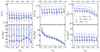 |
Fig. A.1. Accuracy for a 10-yr MPTA in recovering the source parameters as a function of the eccentricity of the detected source, ers: GW amplitude (Δζ/ζ, top left), Keplerian frequency (Δfk/fk, top middle), eccentricity (Δers, top right), inclination angle (Δi, bottom left), the initial phase of the orbit (Δl0, bottom middle), and sky localisation (ΔΩ, bottom right). All the results have been divided into three different S/N bins 3 < S/N < 10 (pale blue), 10 < S/N < 15 (blue) and S/N > 15 (dark blue). |
All Figures
|
Fig. 1. Sky position of the pulsars included in the PTA experiments used in this work. The pulsars from MPTA are displayed in blue whereas the ones of SKA (full PsrPopPY population) are depicted in orange. |
| In the text | |
|
Fig. 2. Sensitivity curves of 10-year MPTA (blue) and 30-year SKA (orange) computed from HASASIA. The vertical dashed lines correspond to the frequency associated with the observing time span of MPTA and SKA (highlighted with vertical dashed lines). For completeness, the square mean of sGWB produced by our MBHB populations at different e0 models are represented in different colors. Pale (dark) blue and orange lines correspond to the MPTA and SKA sensitivity curves when accounting for pulsar white noise only (white plus red noise). |
| In the text | |
|
Fig. 3. Median number of resolvable sources of 96 randomly selected catalogs (Nres), with three diffented initial eccentricity, e0 = 0.0, e0 = 0.5, e0 = 0.9, as a function of the adopted thresholds in the GW signal amplitude (hth). Each set of marks and colors represents populations with different e0, as labeled in the figure. The values of Nres are computed by using the SKA PTA. |
| In the text | |
|
Fig. 4. Number of resolvable sources (Nres) for as a function of e0. Open dots represent median values from all the considered MBHB population models, while error bars represent the 84 and 16 percentile of the distribution. Blue points correspond to the results of 10-year MPTA data with S/N > 3, while the red ones represent the predictions for 30-year SKA data with S/N > 5. Orange points represent the 30-year SKA results but when accounting only for the white pulsar noise. The lower panel shows the eccentricity distribution of the whole MBHB population for different e0 models (black) and the eccentricity distribution of the MBHBs detectable as CGW sources (ers) for SKA PTA (red) and for MPTA (blue). We note that all the distributions are normalised to the same peak value for visualisation purposes. |
| In the text | |
|
Fig. 5. Cumulative distribution function (CDF) of the S/N featured by MBHBs detected by 30-year SKA PTA. Blue, orange, and purple curves represent the CDF of all the models generated with e0 = 0, 0.5 and 0.9, respectively. The lower panel presents the number of sources found with a given value of S/N for e0 = 0.5 and e0 = 0.9 models (orange and purple line) normalised with the same value found in the e0 = 0 case. |
| In the text | |
|
Fig. 6. Characteristic strain (hc) as a function of observed frequency (f). The upper panel shows a binary with ℳ ∼ 108.5 M⊙ and the observed Keplerian frequency fk ∼ 10−8 Hz; while the lower panel shows a binary of ℳ ∼ 1010 M⊙ and fk ∼ 10−9.5 Hz outside the SKA PTA sensitivity curve. In each panel, blue, orange, and purple lines represent the root mean square of the sGWB generated by all the models with e0 = 0, 0.5 and 0.9, respectively. The black line corresponds to the sensitivity curve of SKA PTA (white and red noise) 30-year data. The colored dots represent how the signal of an MBHB is distributed across different frequencies when the eccentricity is varied between 0, 0.5 and 0.9. |
| In the text | |
|
Fig. 7. Chirp mass distribution (ℳ, upper left panel), redshift (z, upper right panel), twice the observed Keplerian frequency (f2, lower left panel), and inclination angle (i, lower right panel) of the detected MBHBs. Each color represents the distributions when different eccentricity values are used to evolve the MBHB population (e0 = 0, blue, e0 = 0.5, orange and e0 = 0.9 purple). NBin represents the number of objects in a given bin of the histogram while Ntot is the total number of objects analyzed. While the upper panels represent the results for 30-year SKA PTA, the lower ones correspond to 10-year MPTA. |
| In the text | |
|
Fig. 8. Accuracy in recovering the source parameters as a function of the eccentricity of the detected source, ers: GW amplitude (Δζ/ζ, top left), Keplerian frequency (Δfk/fk, top middle), eccentricity (Δers, top right), inclination angle (Δι, bottom left), the initial phase of the orbit (Δl0, bottom middle) and sky localisation (ΔΩ, bottom right). All the results have been divided into three different S/N bins 3 < S/N < 10 (orange), 10 < S/N < 15 (dark orange), and S/N > 15 (dark red). |
| In the text | |
|
Fig. 9. Probability distribution function (PDF) of 𝒟f for binaries featuring h > hth (top panel) and binaries detected by SKA PTA (S/N > 5, bottom panel). In both panels, green lines correspond to the cumulative distribution function (CDF). |
| In the text | |
|
Fig. 10. Probability distribution function (PDF) of 𝒟γ for binaries featuring h > hth (top panel) and binaries detected by SKA PTA (S/N > 5, bottom panel). In both panels, blue lines correspond to the cumulative distribution function (CDF). |
| In the text | |
|
Fig. A.1. Accuracy for a 10-yr MPTA in recovering the source parameters as a function of the eccentricity of the detected source, ers: GW amplitude (Δζ/ζ, top left), Keplerian frequency (Δfk/fk, top middle), eccentricity (Δers, top right), inclination angle (Δi, bottom left), the initial phase of the orbit (Δl0, bottom middle), and sky localisation (ΔΩ, bottom right). All the results have been divided into three different S/N bins 3 < S/N < 10 (pale blue), 10 < S/N < 15 (blue) and S/N > 15 (dark blue). |
| In the text | |
Current usage metrics show cumulative count of Article Views (full-text article views including HTML views, PDF and ePub downloads, according to the available data) and Abstracts Views on Vision4Press platform.
Data correspond to usage on the plateform after 2015. The current usage metrics is available 48-96 hours after online publication and is updated daily on week days.
Initial download of the metrics may take a while.