| Issue |
A&A
Volume 628, August 2019
|
|
|---|---|---|
| Article Number | A17 | |
| Number of page(s) | 9 | |
| Section | Extragalactic astronomy | |
| DOI | https://doi.org/10.1051/0004-6361/201834573 | |
| Published online | 29 July 2019 | |
Gaia GraL: Gaia DR2 gravitational lens systems
IV. Keck/LRIS spectroscopic confirmation of GRAL 113100−441959 and model prediction of time delays
1
Argelander-Institut für Astronomie, Universität Bonn, Auf dem Hügel 71, 53121 Bonn, Germany
e-mail: This email address is being protected from spambots. You need JavaScript enabled to view it.
2
Jet Propulsion Laboratory, California Institute of Technology, 4800 Oak Grove Drive, Pasadena, CA 91109, USA
3
CENTRA, Faculdade de Ciências, Universidade de Lisboa, Ed. C8, Campo Grande, 1749-016 Lisboa, Portugal
4
Institut d’Astrophysique et de Géophysique, Université de Liège, 19c, Allée du 6 Août, 4000 Liège, Belgium
5
Laboratoire d’Astrophysique de Bordeaux, Univ. Bordeaux, CNRS, B18N, allée Geoffroy Saint-Hilaire, 33615 Pessac, France
6
Université Côte d’Azur, Observatoire de la Côte d’Azur, CNRS, Laboratoire Lagrange, Boulevard de l’Observatoire, CS 34229, 06304 Nice, France
7
Instituto de Astronomia, Geofísica e Ciências Atmosféricas, Universidade de São Paulo, Rua do Matão, 1226, Cidade Universitária, 05508-900 São Paulo, SP, Brazil
8
Zentrum für Astronomie der Universität Heidelberg, Astronomisches Rechen-Institut, Mönchhofstr. 12-14, 69120 Heidelberg, Germany
9
California Institute of Technology, 1200 E. California Blvd, Pasadena, CA 91125, USA
10
International Space Science Institute (ISSI), Hallerstraße 6, 3012 Bern, Switzerland
11
School of Physics, The University of Sydney, NSW 2006, Australia
12
Niels Bohr Institute – Københavns Universitet, Juliane Maries Vej 30, 2100 Copenhagen, Denmark
13
School of Physics & Astronomy, North Haugh, St Andrews, UK
14
Universität Hamburg, Faculty of Mathematics, Informatics and Natural Sciences, Department of Earth Sciences, Meteorological Institute, Bundesstraße 55, 20146 Hamburg, Germany
Received:
5
November
2018
Accepted:
23
January
2019
Abstract
We report the spectroscopic confirmation and modeling of the quadruply imaged quasar GRAL 113100–441959, the first gravitational lens (GL) to be discovered from a machine learning technique that only relies on the relative positions and fluxes of the observed images without considering colour informations. Follow-up spectra obtained with Keck/LRIS reveal the lensing nature of this quadruply imaged quasar with redshift zs = 1.090 ± 0.002, but show no evidence of the central lens galaxy. Using the image positions and G-band flux ratios provided by Gaia Data Release 2 as constraints, we modeled the system with a singular power-law elliptical mass distribution (SPEMD) plus external shear, to different levels of complexity. We show that relaxing the isothermal constraint of the SPEMD does not lead to statistically significant different results in terms of fitting the lensing data. We thus simplified the SPEMD to a singular isothermal ellipsoid to estimate the Einstein radius of the main lens galaxy θE = 0.″851, the intensity and position angle of the external shear (γ,θγ) = (0.044, 11.°5), and we predict the lensing galaxy position to be (θgal,1, θgal,2) = (−0.″424, −0.″744) with respect to image A. We provide time delay predictions for pairs of images, assuming a plausible range of lens redshift values zl between 0.5 and 0.9. Finally, we examine the impact on time delays of the so-called source position transformation, a family of degeneracies existing between different mass density profiles that reproduce most of the lensing observables equally well. We show that this effect contributes significantly to the time delay error budget and cannot be ignored during the modeling. This has implications for robust cosmography applications of lensed systems. GRAL 113100–441959 is the first in a series of seven new spectroscopically confirmed GLs discovered from Gaia Data Release 2.
Key words: gravitational lensing: strong / quasars: general / astrometry
© ESO 2019
1. Introduction
Already suspected before general relativity (Einstein 1916), it was only after Einstein’s final formulation of its theory that strong gravitational lensing (GL) was described quantitatively. Then it took no less than three-quarters of a century to obtain a definitive observational proof when Walsh et al. (1979) discovered a pair of quasars separated by 6 arcsec, with identical colors, redshifts, and spectra, thereby confirming the first doubly imaged quasar. Because the study of GLs constitutes a unique tool in various fields of astronomy (see, e.g., Treu & Marshall 2016; Gilman et al. 2018; Jauzac et al. 2018; Zavala et al. 2018; Tagore et al. 2018, and references therein), they are highly sought after, but not without difficulty. Even in this era of all-sky surveys, their discovery remains a great challenge, with barely a few hundred systems currently confirmed. A list of currently known GLs can be found in Ducourant et al. (2018; hereafter Paper II).
Data from the ESA/Gaia space mission (Gaia Collaboration 2016) is expected to change the situation dramatically. Gaia is conducting the largest, most precise, most accurate all-sky astrometric survey from space. Its main goal is to chart a three-dimensional map of our Galaxy based on measurements of parallaxes, proper motions, positions and spectro-photometric parameters for more than a billion stars. With an order of magnitude improvement over typical HST astrometric accuracy, Gaia will also detect ∼600 000 quasars (Mignard 2012; Robin et al. 2012), of which 2900 are expected to be multiply imaged and resolved in the final Gaia Data Release (Gaia DR), including 250 systems with more than two lensed images (Finet & Surdej 2016).
As part of a larger effort to discover and study multiply imaged quasar systems hidden in the heart of the Gaia DRs, the Gaia GraL group has recently developed and successfully applied various techniques to identify new highly probable gravitational lens candidates from Gaia’s data. Our strategy is twofold and can be summarized as follows. Initially, our research focused on all known quasars that we compiled in an up-to-the-minute list populated primarily with the Million Quasars Catalog (Flesch 2015, 2017), searching for the presence in Gaia DR2 of one or more nearby (< 6″) point-like companion(s). This was the initial approach we took in Krone-Martins et al. (2018; hereafter Paper I). Next, we designed a dedicated method to blindly identify clusters of point-like objects from the information available in the Gaia DRs using the hierarchical triangular mesh technique (Kunszt et al. 2001). This was the approach we took in Delchambre et al. (2019; hereafter Paper III).
The list of clusters generated from these two approaches is expected to be polluted with contaminants, resulting primarily from chance alignements of unrelated sources. To discard the most obvious ones, we thus applied soft astrometric filters to differentiate genuine candidates from fortuitous clusters of stars by studying the image proper motions and parallaxes of known lenses, as measured by Gaia (see Paper II). Gaia DR2 also provides broadband photometric measurements in the G-band (330–1050 nm), in particular, a color indicator derived from the integrated flux of the low-resolution blue photometer (BP, 300−680 nm) and red photometer (RP, 630−1050 nm) spectra (Jordi et al. 2010; Evans et al. 2018). Because the GL phenomenon is achromatic, we also rejected clusters for which the individual component BP − RP color indicators significantly differ from each other. With the purpose of considering only the most plausible candidates, we classified the remaining clusters that successfully passed the astrometric and photometric filters with respect to their chance of being a multiply imaged quasar candidate. To this end, we assigned to each of them a probability that reflects the match between a candidate and the learning set composed of more than 108 simulated image configurations that we used to build extremely randomized trees (Geurts et al. 2006). When considering a non-singular isothermal ellipsoid (NIE) plus external shear as the lens model, various tests have shown this method to be efficient in identifying known GLs from fortuitous clusters of stars with a detection probability of 97% in the case of configurations with four lensed images along with a contamination ratio of 1.37%. Implementing this strategy to Gaia DR2, we discovered 15 new highly probable quadruply imaged quasar candidates, recently presented in Paper III. Furthermore in this blind search, we also found 17 well-known quadruply imaged quasars for which three or four components are detected in Gaia DR2. This constitutes additional evidence of the robustness of our methodology.
GRAL 113100–441959 was identified for the first time as a new highly probable GL candidate in Paper I, and was then rediscovered independently with an ERT probability of 96% from the blind search technique presented in Paper III (candidate number [12] their Fig. 3). This is likely the first gravitationally lensed quasar discovered from astrometric and photometric survey data. Prior to its spectroscopic confirmation, we were not able to perform any visual inspection of this candidate because the available surveys either lack spatial resolution and/or sensitivity (e.g., SkyMapper, Wolf et al. 2018, and ALLWISE, Wright et al. 2010), or they lack spatial coverage (e.g., Pan-STARRS, Chambers et al. 2016). The limited spatial resolution of current all-sky southern surveys probably explains why GRAL 113100–441959 remained unnoticed thus far, confirming that many GLs that can be observed from the ground are yet to be discovered.
In Sect. 2 we describe the spectroscopic observations and confirm the lensing nature of GRAL 113100–441959. In Sect. 3, we describe the detail of the simple lens modeling, and provide predictions for the time delays between pairs of lensed images in Sect. 4. Finally, we summarize our findings and conclude in Sect. 5.
2. Lens confirmation
2.1. Observations
On UT 2018 May 13, we observed GRAL 113100–441959 with the dual-beam Low Resolution Imaging Spectrometer (Oke et al. 1995) on the Keck I telescope. The conditions were photometric, and we obtained two 300 s spectra, at position angles (PAs) of 60° and 135°. We used the 1″ width slit, the 5600 Å dichroic, the 600 ℓ mm−1 blue grism (λblaze = 4000 Å), and the 400 ℓ mm−1 red grating (λblaze = 8500 Å). This instrument configuration covers the full optical window at moderate resolving power, R ≡ λ/Δλ ≈ 1100. The observations were processed using standard techniques within IRAF, and flux-calibrated using observations of the spectrophotometric white dwarf standard stars Feige 34, Feige 67, and Wolf 1346 obtained on the same night.
The target appears as a single source in the PA = 135° observation, which was aligned along the brighter NE components of the lens. Though the two components are not differentiated in the spectroscopy, the source is clearly spatially resolved, with a FWHM of  compared to the
  seeing.
In the PA = 60° observation, the target is clearly resolved into two sources separated by  with identical spectroscopic features. One component is significantly brighter than the other. Figure 1 presents the spectra of the brighter (NE) and fainter (SW) components, each extracted with
  box width. Based on Gaussian fits to the typical broad quasar emission lines such as C III] λ1909, Mg II λ2800, and Balmer transitions of hydrogen, we measured a redshift of z = 1.090 with a conservative estimate of the uncertainty of 0.002.
On UT 2018 July 31, GRAL 113100–441959 was also observed with the  Two Color Instrument (TCI) Lucky imager (Evans et al. 2016) mounted on the 1.54 m Danish telescope at La Silla, Chile. A sequence of eight spools of two minute exposures was obtained with the RED color channel. We combined all the quality bins of each spool to generate the 16 min total exposure image shown in Fig. 2.
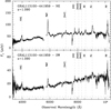 |
Fig. 1. Keck/LRIS spectra of images (A+B) and (C+D) at position angle 60°. Dashed lines identify emission lines used to confirm the lensing nature of GRAL 113100–441959. |
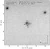 |
Fig. 2. First direct imaging of GRAL 113100–441959 obtained with the DK-1.54/TCI Lucky imager during the night of UT 2018 July 31 (on-site observer: Martin Burgdorf). The black squares locate the lensed imaged positions as reported in the Gaia DR2. |
2.2. The lensing nature of GRAL 113100–441959
Figure 1 presents the calibrated spectra of GRAL 113100–441959 from the PA = 60° observation; a wide aperture was extracted containing both observed components. The PA = 135° observation is identical to the one we have obtained for PA = 60°. The source is clearly identified as a quasar at zs = 1.090 based on strong detections of broad emission from C III] λ1909, Mg II λ2800, Hγ and Hβ. In addition, narrow, forbidden transitions of oxygen and highly ionized neon are also evident. These features, seen in both components of the PA = 60° spectra, clearly confirm the lensing nature of GRAL 113100–441959. There is no clear evidence of the lensing galaxy in the Keck data, neither in the sky-subtracted two-dimensional spectra, nor in the extracted, calibrated one-dimensional spectra.
3. Lens modeling
In this section, we describe the method applied to obtain a simple lens model that can adequately reproduce the lensing observables provided by Gaia DR2. Our motivation is to use this model to predict time delays between pairs of lensed images for a range of plausible lens redshift values.
3.1. Overview
The constraints on the lens mass distribution include the relative angular positions θi of the lensed images with respect to the brighter image (hereafter image A) and the flux ratios fi ≡ Fi/FA in the G-band between the images i and A. Because the number of constraints is quite limited, we reconstructed the lens mass distribution using only a simple physically motivated and fully parametrized model, described in Sect. 3.2.
Both the astrometric and photometric Gaia measurements are affected by statistical errors. However, the flux uncertainties as given in Gaia DR2 do not reflect various well-known sources of uncertainty that have to be taken into account in the modeling scenario, the most important of which are (i) microlensing effects of one or several of the macrolensed images (see, e.g., Wambsganss & Paczynski 1991; Chae et al. 2001; Akhunov et al. 2017), (ii) small scale structures in the lens galaxy at the image positions (Mao & Schneider 1998; Metcalf & Madau 2001; Hsueh et al. 2017, and references therein), (iii) differential dust-reddening (see, e.g., Murphy & Liske 2004; Jean & Surdej 2007; Ménard et al. 2008), and (iv) source variability which propagates into image light curves with lags due to time delays (Treu & Marshall 2016). To represent these unquantified effects, we thus used conservative 15% Gaussian errors for the image flux ratios. Both the lensing observables and their related uncertainties are reported in Table 1. Although the flux ratios may be strongly affected by these sources of uncertainty, their use increases the number of lensing observables. This allows for more flexibility as regards the choice of a lens model capable of capturing different sources of angular structure of the lensing potential.
Gaia’s lensing observables for GRAL 113100–441959.
We performed the modeling using pySPT (Wertz & Orthen 2018), a software package mainly dedicated to the study of the source position transformation (SPT) but which comes with several simple modeling tools, and gravlens, a lensing-dedicated software package developed by C. R. Keeton (Keeton 2001b, 2010, 2011).
3.2. Lens mass models
We modeled the mass distribution of the lens galaxy using a singular power-law elliptical mass distribution (SPEMD), which is broadly consistent with typical lens galaxies and has been extensively used in the literature (see, e.g., Suyu et al. 2009; Sonnenfeld et al. 2013; Birrer et al. 2016; Wong et al. 2017; Shajib et al. 2019). The corresponding dimensionless surface mass density profile, also known as the convergence, is defined by
 (1)
(1)
where θE is the Einstein radius, a the power-law slope1, and q the minor-to-major axis ratio of the elliptical iso-density contours. The on-sky Cartesian angular coordinates (θ1, θ2) are clockwise rotationally transformed into the coordinates  , whose axes are aligned with the minor and major axes of the lens. Specifically, we write
  where R is the rotation matrix and θq the position angle of the minor axis. The SPEMD simplifies into a singular isothermal ellipsoid (SIE) when a = 1, and into a singular isothermal sphere (SIS) when both a = 1 and q = 1. Closed-form expressions for the SPEMD deflection angle α and deflection potential ψ can be found in Keeton (2001a).
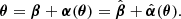
We also included external shear (see, e.g., Meylan et al. 2006) to describe the weak influence of long-scale structure and possible local massive objects. This adds the two parameters γ (shear strength) and θγ (shear position angle) to the lens model. In addition to the model parameters, both the position of the source (β1, β2) and the lens galaxy centroid (θgal, 1, θgal, 2) are also unknown quantities. A first estimate may, however, be inferred from the centroid of the four lensed image positions, namely  with respect to the image A, which has been used as a prior for both (β1, β2) and (θgal, 1, θgal, 2).
3.3. Modeling procedure
For a given lens model, the model parameter space is in general populated with several isolated local minima in the χ2-map. As a first step, we thus explored the parameter space using the differential evolution algorithm (Storn & Price 1997), which is designed to search for the global solution with no absolute guarantee to find it. A benefit of this method is that it requires no initial solution, only ranges of parameter values. We defined half the largest angular separation θmax between the images as a prior for θE, and considered the initial range [θmax/4, 4θmax]. For both the source position and lens galaxy centroid, we set the initial range [cj − θmax/2, cj + θmax/2] for each coordinate (j = 1, 2). We also set the initial ranges q ∈ [0.1, 1.0], γ ∈ [0.0, 0.3], a ∈ [0.5, 1.5], and [0, 2π] for the two angular parameters θq and θγ.
For this first step, we focused primarily on finding lens models that can reproduce the lensed image positions, and ignored the contribution of the observed flux ratios when defining the cost function to minimize. We defined the latter as the dispersion of the sources βi ≡ β(θobs, i, p) = θobs, i − α(θobs, i), which are traced back from the observed image positions θobs for a given set of parameters p. Because it does not require the lens equation to be solved, calculating βi is very efficient. We obtained a first set of parameters p0, which includes the SPEMD model parameters, the lens galaxy centroid, and the source position β0 derived from the mean value of βi resulting from the best fit. To decrease the chance of getting stuck in a local solution, we also ran the minimization process on subregions of the parameter space, and compared the subresults with the one obtained when running on the entire parameter space. Finally, we also used the flux ratios which have so far remained unused, as an additional constraint to separate plausible from poor local solutions. To this end, we merely compared the model-predicted image flux ratios to the observed ones, and discarded the local solutions showing differences Δf = |fi − fobs, i| larger than 0.3 (2σf), for at least one image.
As a second step, we refined the solution using a downhill simplex algorithm (Nelder & Mead 1965) with p0 as the first guess, and included the contribution of the image flux ratios explicitly in the cost function to minimize. Assuming that the errors follow a Gaussian distribution, the goodness of the fit was evaluated with a reduced χ2 statistics,  , where Nd.o.f. represents the number of degrees of freedom, naively defined as the difference between the number of lensing observables and that of the model free parameters (Andrae et al. 2010). The χ2 statistic results from the sum of the two contributions
  and
and  , characterized by
 (2)
(2)
where θobs and θ are respectively the observed and model-predicted positions of the lensed images, fobs and f are the observed and model-predicted flux ratios, and σ their associated uncertainties.
We initiated the modeling procedure by fixing the parameters a = 0 and q = 1, and successively increased the model complexity. We tested the statistical significance of including these parameters using an F-test (see, e.g., Bevington 1969). Following Cohn et al. (2001) and Protassov et al. (2002), we recall that adding a parameter to a given model is statistically significant, with a confidence level 0 < ν < 1 compared to the improvement expected for a random variable, if the difference between the χ2 statistics, |Δχ2| > h χ2/Nd.o.f., exceeds the reduced χ2 obtained for the unmodified model by a factor h = ppf(ν, ΔNd.o.f., Nd.o.f.)/ΔNd.o.f., where ppf is the so-called percent point function of the F-distribution (David 1949; Pearson 1951). For instance, if adding one parameter to a model having Nd.o.f. = 4 improves the fit from χ2 = 21.1 to 3.5, one obtains |Δχ2| = 17.6 ≥ 6.79 = (21.1/4) × ppf(0.68, 1, 4), and the F-test suggests that adopting the new model is statistically justified under the 1σ confidence level hypothesis. Similarly, one can compute the confidence level ν⋆ for which |Δχ2| = h χ2/Nd.o.f., and compare it with the 1σ confidence level ν1σ ≃ 0.68 = 68%. In our example, one has ν⋆ ≃ 86% > ν1σ, which leads to the same conclusion.
As a third step, we further explored the parameter space of the best fit model and deduced confidence intervals for each model parameter using a Bayesian inference method based on a Monte-Carlo Markov chain (MCMC) sampling. We sampled the posterior probability distribution function (pdf) of the model parameters using emcee (Foreman-Mackey et al. 2013), a Python package which implements the affine-invariant ensemble sampler for MCMC proposed by Goodman & Weare (2010). We monitored the chains, also called walkers, using the fraction of accepted to proposed candidates (the so-called acceptance rate, Mackay 2003), and assessed the convergence with the integrated autocorrelation time (Christen & Fox 2010; Goodman & Weare 2010), which gives an estimate of the number of posterior pdf evaluations required to draw an independent sample. We then computed the 1σ confidence intervals from the 16th and 84th percentiles.
3.4. Model properties
We first examined the SPEMD with a = 1 and q = 1 in an external shear field, hereafter denoted as the SISg model. This model is characterized by seven parameters (θE, γ, θγ, β1, β2, θgal, 1, θgal, 2) and Nd.o.f. = 4. With χ2/Nd.o.f. = (89.3 + 1.3)/4, the SISg model poorly fits the data, in particular the image positions. Although this result comes as no surprise considering the incredible simplicity of the SISg model, it provides a first estimate of the Einstein radius,  , and of the external shear,
  , see Table 2. Adding an ellipticity (q, θq) parameter to the SISg, thus transforming it into a SIEg, considerably improves the fit to χ2/Nd.o.f. = (0.0 + 1.2)/2, and is statistically significant with a confidence level ν⋆ = 75% (>68%) for the F-test. Letting the parameter a vary during the optimization process, we relaxed the isothermal hypothesis. This slightly improves the fit, χ2/Nd.o.f. = (0.0 + 1.1)/1, but is not statistically significant according to the F-test (ν⋆ = 28%). Increasing the model complexity favors slightly higher ellipticity (1 − q) along with smaller external shear strength. This clearly reflects the well-known degeneracy existing between these two sources of angular structure (see, e.g., Keeton et al. 1997; Keeton 2010; Kneib & Natarajan 2011).
Best-fit model parameters obtained for the three complexity levels of the SPEMD plus external shear.
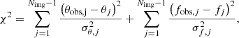
The errors σf adopted for the image flux ratios are to some extent arbitrary. We thus explored the impact on the fit when we modify these values. In this regard, we restrained ourselves to estimate these errors by rescaling σf to artificially obtain  , because this method has been shown to be incorrect (e.g., Andrae 2010). We found that the SIEg remains the one providing the most statistically significant results. As a next step, we sampled the pdfs for all SIEg parameters, using the best fit parameter values reported in Table 2 to initialize 250 walkers. The resulting pdfs and the correlation between model parameters are represented with two corner plots, in Figs. 3 and 4 respectively. The corresponding confidence intervals are also reported in Table 2. As expected, the shear-ellipticity degeneracy induces a significant correlation between the parameters (γ, θγ) and (q, θq). In Fig. 5, we represent the lensed image configuration, labeled from A to D, on top of a few predicted lensing quantities for the SIEg model reported in Table 2. The predicted mass within a circular aperture of radius θE is estimated to be in the range M(≤θE) = 2.498 ± 0.003 × 10¹¹ M⊙ for zl = 0.5 and M(≤θE) = 1.119 ± 0.002 × 10¹² M⊙ for zl = 0.9.
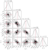 |
Fig. 3. Results of MCMC sampling for the SIEg model parameters. The diagonal panels illustrate the posterior pdfs while the off-axis ones illustrate the correlation between the parameters. The vertical red lines and red crosses correspond to the best solution obtained from the down-hill simplex algorithm and used to initiate the 250 walkers. The vertical dashed lines locate the 16th and 84th percentiles. |
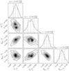 |
Fig. 4. Results of the MCMC sampling for the source position and lens galaxy centroid. The diagonal panels illustrate the posterior pdfs while the off-axis ones illustrate the correlation between the parameters. The vertical dashed lines locate the 16th and 84th percentiles. |
 |
Fig. 5. GRAL 113100−441959 image configuration. The black dots locate the image positions, and their size mimics the associated flux, as reported in the Gaia DR2. The solid line represents the tangential critical line, the diamond-shaped dashed line represents the corresponding caustic line, and the dotted line defines the direction of the external shear. Finally, the color map shows how the surface mass density κ is distributed. |
The axis ratio  agrees within 2σ with the value Wynne & Schechter (2018) obtained using Witt’s hyperbola. The slight disprecancy may be explained by the fact that they used different astrometric positions they derived from Dark Energy Camera (DECam) observations. Furthermore, these observations reveal the presence of the lens galaxy, the centroid of which should be determined (priv. comm.).
4. Model-predicted time delays
From the set of highly probable lens models obtained from the MCMC sampling, we computed the predicted time delays Δtij between pairs of images (θi, θj), which are defined by
![Mathematical equation: $$ \begin{aligned} \Delta t_{ij} = \frac{D_{\Delta t}}{c}\left[\frac{1}{2}\left(|\boldsymbol{\alpha }({\boldsymbol{\theta }}_i)|^2-|\boldsymbol{\alpha }({\boldsymbol{\theta }}_j)|^2\right) - (\psi ({\boldsymbol{\theta }}_i) - \psi ({\boldsymbol{\theta }}_j)) \right] , \end{aligned} $$](/articles/aa/full_html/2019/08/aa34573-18/aa34573-18-eq51.gif) (3)
(3)
where  is the time delay distance, with D the angular diameter distance between the observer and lens (Dl), observer and source (Ds), and lens and source (Dls). The angular diameter distance depends only on the redshift and the cosmology. From the Keck/LRIS spectra, the redshift of the source was found to be zs = 1.09. However, as there is no clear evidence of the lensing galaxy in the Keck/LRIS spectral data, we were prevented from determining its redshift zl (see Sect. 2.2). We thus computed the time delay distance, hence the time delays, for a set of lens redshifts in the plausible range zl ∈ [0.5, 0.9]. We adopted the ΛCDM model along with the final Planck 2018 results (Planck Collaboration VI 2018). The normalized Δtij h−1 against the lens redshift zl is shown in Fig. 6, in which the factor h is used to calibrate the Hubble constant H0 = 100 h km s−1 Mpc−1.
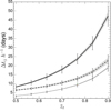 |
Fig. 6. Model-predicted time delays scaled with h. The error bars combine the three sources of uncertainties described in the text. The gray shaded regions depict the contribution of the SPT to the error budget. The solid line corresponds to images C−D, the dashed line to C−A, and the dotted line to C−B. For the sake of clarity, we shifted upwards the time delays between images C−A (dashed line) by a three-day offset. |
The error budget associated with Δtij was estimated by considering three sources of uncertainties. Firstly, we propagated the statistical error inferred from the MCMC sampling. This was simply done by constructing histograms for Δtij h−1 from the independent samples of SIEg model parameters reported in Figs. 3 and 4. An example of these histograms is illustrated in Fig. 7 for the case of zl = 0.7. Secondly, we considered the impact of hypothetical massive objects lying on the line-of-sight by scaling the theoretical time delay distance with an external convergence term κext such that 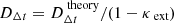 (see, e.g., Keeton 2003). We applied a different scaling for each set of model parameters used to construct the histograms (see Fig. 7). The κext values were randomly drawn from a zero mean normal distribution and characterized by a conservative standard deviation σκ = 0.03 (see, e.g., Wong et al. 2017). When combined, the typical errors are ∼7.7% for ΔtCB, ∼7.8% for ΔtCA, and ∼7.6% for ΔtCD, compared to the median values. Thirdly, we considered the impact of the Source Position Transformation (SPT), a degeneracy existing between different lens density profiles that reproduce equally well the lensing observables, except for the product Δt H0 (Schneider & Sluse 2013, 2014). A short summary is given in Appendix A. We SPT-transformed the SIEg model using the modified deflection law
 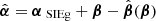 along with a radial stretching of the source plane defined by
 ![Mathematical equation: $ {\hat{\boldsymbol{\beta}}}(\boldsymbol{\beta}) = [1 + f(|\boldsymbol{\beta}|)]\ \boldsymbol{\beta} $](/articles/aa/full_html/2019/08/aa34573-18/aa34573-18-eq55.gif) . In particular, we considered the special case where the deformation function f(|β|) is the lowest-order expansion of more general functions, f(|β|) = f0 + f2|β|2/(2θE), where the constants f0 = f(0) and
. In particular, we considered the special case where the deformation function f(|β|) is the lowest-order expansion of more general functions, f(|β|) = f0 + f2|β|2/(2θE), where the constants f0 = f(0) and  quantify the magnitude of the deformation. This choice explores a large variety of degeneracies characterized by an isotropic transformation of the source plane. In the end, this at least defines a lower limit on the impact of the SPT on the time delays. In the particular case of f2 = 0, the SPT reduces to the well-known mass-sheet degeneracy (MSD) characterized by
 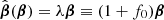 . In our analysis, we only explored degeneracies that cannot be explained by a MSD, hence f0 = 0.
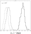 |
Fig. 7. Example of histograms for Δtij h−1 constructed for zl = 0.7 from the MCMC results. The solid line corresponds to images C−D, the dashed line to C−A, and the dotted line to C−B. |
As previously defined,  is not a curl-free field, and hence does not correspond to the deflection produced by a gravitational lens. To overcome this hurdle, one can (i) derive the closest curl-free approximation to
  in a circular region of the lens plane as proposed in Unruh et al. (2017) and applied in Wertz et al. (2018) and Wertz & Orthen (2018), or (ii) extract the curl-free part from
  using an Helmholtz-Hodge decomposition (Helmholtz 1858). In both cases, the new deflection law is denoted
  . We adopted the Helmholtz-Hodge decomposition strategy, given that the region of interest can be straightforwardly reduced to the annulus that includes all four images, leading to higher predicted time delay deviations than found with the first approach (Wertz & Schneider, in prep.). The higher the value of f2, the larger deformation of the source plane along with the deflection law
  , hence the larger deviations of the predicted image positions in comparison with the observations. For each set of the SIEg model parameters, we thus computed the highest acceptable f2 value, which guarantees the corresponding SPT-transformed model to produce an image configuration identical to the one observed by Gaia, within the astrometric and photometric error bars. For the best fit SIEg model reported in Table 2, we found |f2| = 1.67, which is representative of the values we obtained for the entire sample. We then repeated the process for the different lens redshifts. Finally, the impact of the SPT results in additional time delay deviations of 2.7% for ΔtCB, 7.7% for ΔtCA, and 4.1% for ΔtCD. This contribution corresponds to a significant fraction of the time delay error budget, in particular for ΔtCA where the SPT input reaches the same level as the statistical errors. We finally combined the three different sources of uncertainties to obtain the error bars displayed in Fig. 6.
As a result, the model-predicted time delays vary from (for zl = 0.5) ΔtCA h−1 = 3.48 ± 0.54 days, ΔtCB h−1 = 3.32 ± 0.35 days, and ΔtCD h−1 = 8.35 ± 0.98 days, to (zl = 0.9) ΔtCA h−1 = 19.75 ± 3.07 days, ΔtCB h−1 = 18.83 ± 2.00 days, and ΔtCD h−1 = 47.42 ± 5.61 days.
5. Conclusions
This paper presents the spectroscopic confirmation of the gravitationally lensed quasar GRAL 113100–441959, previously identified in Paper I as a highly probable GL candidate hidden in the Gaia DR2. We obtain Keck/LRIS spectroscopy on the night of UT 2018 May 13, revealing similar spectra for the combinations of sources A+B and C+D, for the slit at a position angle of 60°, and A+B and C+D for the slit at a position angle of 135°. We confirm the lensing nature of GRAL 113100–441959 by clearly identifying several similar emission spectral lines between the images (A+B) and (C+D), and measured redshits for these combination of lensed images of the quasar as zs = 1.09.
We modeled the main lens galaxy with a SPEMD plus external shear, and explored different levels of model complexity. This study indicates that the SIEg model (which is equivalent to SPEMD with a = 1) is the best choice in terms of goodness of the fit and statistical significance, given the available observational data. We infer the confidence intervals for each model parameter using a Bayesian inference method based on a MCMC sampling. We find  for the Einstein radius. The lens galaxy ellipticity is inferred to have an axis ratio of
 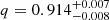 pointing to
  east of north. The shear strength is found to be moderate, γ = 0.044 ± 0.002, pointing
  east of north. This suggests that the ellipticity captures most of the source of angular structure. Finally, we predict the lensing galaxy to lie at
  from image A.
We also used the MCMC results to predict the three independent time delays between pairs of images. As the redshift zl of the lensing galaxy is still unknown, we provide the model-predicted time delays for a range of physically plausible zl, between 0.5 and 0.9. Finally, we assessed the error affecting our estimation, and in particular quantified the impact of the SPT. We find that the contribution of the SPT to the error budget cannot be ignored for precise applications of strongly lensed systems, as it can be as important as the other uncertainty sources. In the case of GRAL 113100–441959, SPT is extremely relevant for the time delay between the C−A images.
GRAL 113100–441959 is the first spectroscopically confirmed GL from the Gaia GraL sample of highly probable candidates recently presented in Papers I and III of this series. At the time we release this work, nine additional candidates from Paper III were already observed with the Keck/LRIS in other campaigns, with six of them being very likely lenses; the analysis of these other GL candidates will be presented in a companion paper.
The power-law slope a is linked to the three-dimensional slope γ′ of the power-law mass distribution through the relation a = 3 − γ′.
Acknowledgments
The authors would like to thank Paul Schechter for valuable discussions. OW is supported by the Humboldt Research Fellowship for Postdoctoral Researchers. The work of DS was carried out at the Jet Propulsion Laboratory, California Institute of Technology, under a contract with NASA. AKM acknowledges the support from the Portuguese Fundação para a Ciência e a Tecnologia (FCT) through grants SFRH/BPD/74697/2010, PTDC/FIS-AST/31546/2017, from the Portuguese Strategic Program UID/FIS/00099/2013 for CENTRA, from the ESA contract AO/1-7836/14/NL/HB and from the Caltech Division of Physics, Mathematics and Astronomy for hosting a research leave during 2017–2018, when this paper was partially prepared. AKM additionally acknowledges that this research was partially supported by the Munich Institute for Astro- and Particle Physics (MIAPP) of the DFG cluster of excellence “Origin and Structure of the Universe”. LD and JS acknowledge support from the ESA PRODEX Program “Gaia-DPAC QSOs” and from the Belgian Federal Science Policy Office. SGD and MJG acknowledge a partial support from the NSF grants AST-1413600 and AST-1518308, and the NASA grant 16-ADAP16-0232. We acknowledge partial support from “Actions sur projet INSU-PNGRAM”, and from the Brazil-France exchange programs Fundação de Amparo à Pesquisa do Estado de São Paulo (FAPESP) and Coordenação de Aperfeiçoamento de Pessoal de Nível Superior (CAPES) – Comité Français d’Évaluation de la Coopération Universitaire et Scientifique avec le Brésil (COFECUB). This work has made use of the computing facilities of the Laboratory of Astroinformatics (IAG/USP, NAT/Unicsul), whose purchase was made possible by the Brazilian agency FAPESP (grant 2009/54006-4) and the INCT-A, and we thank the entire LAi team, specially Carlos Paladini, Ulisses Manzo Castello, Luis Ricardo Manrique and Alex Carciofi for the support. This work has made use of results from the ESA space mission Gaia, the data from which were processed by the Gaia Data Processing and Analysis Consortium (DPAC). Funding for the DPAC has been provided by national institutions, in particular the institutions participating in the Gaia Multilateral Agreement. The Gaia mission website is: http://www.cosmos.esa.int/gaia. Some of the authors are members of the Gaia Data Processing and Analysis Consortium (DPAC).
References
- Akhunov, T. A., Wertz, O., Elyiv, A., et al. 2017, MNRAS, 465, 3607 [NASA ADS] [CrossRef] [Google Scholar]
- Andrae, R. 2010, ArXiv e-prints [arXiv:1009.2755] [Google Scholar]
- Andrae, R., Schulze-Hartung, T., & Melchior, P. 2010, ArXiv e-prints [arXiv:1012.3754] [Google Scholar]
- Bevington, P. R. 1969, Data Reduction and Error Analysis for the Physical Sciences (New York: McGraw-Hill), 154 [Google Scholar]
- Birrer, S., Amara, A., & Refregier, A. 2016, JCAP, 8, 020 [NASA ADS] [CrossRef] [Google Scholar]
- Chae, K.-H., Turnshek, D. A., Schulte-Ladbeck, R. E., Rao, S. M., & Lupie, O. L. 2001, ApJ, 561, 653 [NASA ADS] [CrossRef] [Google Scholar]
- Chambers, K. C., Magnier, E. A., Metcalfe, N., et al. 2016, ArXiv e-prints [arXiv:1612.05560] [Google Scholar]
- Christen, J. A., & Fox, C. 2010, Bayesian Anal., 5, 263 [CrossRef] [Google Scholar]
- Cohn, J. D., Kochanek, C. S., McLeod, B. A., & Keeton, C. R. 2001, ApJ, 554, 1216 [NASA ADS] [CrossRef] [Google Scholar]
- David, F. N. 1949, Biometrika, 36, 394 [CrossRef] [Google Scholar]
- Delchambre, L., Krone-Martins, A., Ducourant, C., et al. 2019, A&A, 622, A165 (Paper III) [NASA ADS] [CrossRef] [EDP Sciences] [Google Scholar]
- Ducourant, C., Wertz, O., Krone-Martins, A., et al. 2018, A&A, 618, A56 (Paper II) [NASA ADS] [CrossRef] [EDP Sciences] [Google Scholar]
- Einstein, A. 1916, Ann. Phys., 354, 769 [Google Scholar]
- Evans, D. F., Southworth, J., Maxted, P. F. L., et al. 2016, A&A, 589, A58 [NASA ADS] [CrossRef] [EDP Sciences] [Google Scholar]
- Evans, D. W., Riello, M., Angeli, F. De, et al. 2018, A&A, 616, A4 [NASA ADS] [CrossRef] [EDP Sciences] [Google Scholar]
- Finet, F., & Surdej, J. 2016, A&A, 590, A42 [NASA ADS] [CrossRef] [EDP Sciences] [Google Scholar]
- Flesch, E. W. 2015, PASA, 32, e010 [NASA ADS] [CrossRef] [Google Scholar]
- Flesch, E. W. 2017, VizieR Online Data Catalog: VII/280 [Google Scholar]
- Foreman-Mackey, D., Hogg, D. W., Lang, D., & Goodman, J. 2013, PASP, 125, 306 [CrossRef] [Google Scholar]
- Gaia Collaboration (Prusti, T., et al.) 2016, A&A, 595, A1 [NASA ADS] [CrossRef] [EDP Sciences] [Google Scholar]
- Geurts, P., Ernst, D., & Wehenkel, L. 2006, Mach. Learn., 63, 3 [Google Scholar]
- Gilman, D., Birrer, S., Treu, T., & Keeton, C. R. 2018, MNRAS, 481, 819 [NASA ADS] [CrossRef] [Google Scholar]
- Goodman, J., & Weare, J. 2010, Appl. Math. Comput. Sci., 5, 65 [Google Scholar]
- Helmholtz, H. 1858, J. für die reine und angewandte Mathematik, 1858, 25 [CrossRef] [Google Scholar]
- Hsueh, J.-W., Oldham, L., Spingola, C., et al. 2017, MNRAS, 469, 3713 [NASA ADS] [CrossRef] [Google Scholar]
- Jauzac, M., Harvey, D., & Massey, R. 2018, MNRAS, 477, 4046 [NASA ADS] [CrossRef] [Google Scholar]
- Jean, C., & Surdej, J. 2007, A&A, 471, 807 [NASA ADS] [CrossRef] [EDP Sciences] [Google Scholar]
- Jordi, C., Gebran, M., Carrasco, J. M., et al. 2010, A&A, 523, A48 [NASA ADS] [CrossRef] [EDP Sciences] [Google Scholar]
- Keeton, C. R. 2001a, ArXiv e-prints [arXiv:astro-ph/0102341] [Google Scholar]
- Keeton, C. R. 2001b, ArXiv e-prints [arXiv:astro-ph/0102340] [Google Scholar]
- Keeton, C. R. 2003, ApJ, 584, 664 [NASA ADS] [CrossRef] [Google Scholar]
- Keeton, C. R. 2010, Gen. Relat. Grav., 42, 2151 [Google Scholar]
- Keeton, C. R. 2011, Astrophysics Source Code Library [record ascl:1102.003] [Google Scholar]
- Keeton, C. R., Kochanek, C. S., & Seljak, U. 1997, ApJ, 482, 604 [NASA ADS] [CrossRef] [Google Scholar]
- Kneib, J.-P., & Natarajan, P. 2011, A&ARv, 19, 47 [NASA ADS] [CrossRef] [Google Scholar]
- Krone-Martins, A., Delchambre, L., Wertz, O., et al. 2018, A&A, 616, L11 (Paper I) [NASA ADS] [CrossRef] [EDP Sciences] [Google Scholar]
- Kunszt, P. Z., Szalay, A. S., & Thakar, A. R. 2001, in Mining the Sky, eds. A. J. Banday, S. Zaroubi, & M. Bartelmann, 631 [CrossRef] [Google Scholar]
- Mackay, D. J. C. 2003, Information Theory, Inference and Learning Algorithms (Cambridge, UK: Cambridge University Press), 640 [Google Scholar]
- Mao, S., & Schneider, P. 1998, MNRAS, 295, 587 [NASA ADS] [CrossRef] [Google Scholar]
- Ménard, B., Nestor, D., Turnshek, D., et al. 2008, MNRAS, 385, 1053 [NASA ADS] [CrossRef] [Google Scholar]
- Metcalf, R. B., & Madau, P. 2001, ApJ, 563, 9 [NASA ADS] [CrossRef] [Google Scholar]
- Meylan, G., Jetzer, P., North, P., et al. 2006, Gravitational Lensing: Strong, Weak and Micro (Berlin: Springer-Verlag) [Google Scholar]
- Mignard, F. 2012, Mem. Soc. Astron. It., 83, 918 [NASA ADS] [Google Scholar]
- Murphy, M. T., & Liske, J. 2004, MNRAS, 354, L31 [NASA ADS] [CrossRef] [Google Scholar]
- Nelder, J. A., & Mead, R. 1965, Comput. J., 7, 308 [Google Scholar]
- Oke, J. B., Cohen, J. G., Carr, M., et al. 1995, PASP, 107, 375 [NASA ADS] [CrossRef] [Google Scholar]
- Pearson, E. S. 1951, Biometrika, 38, 257 [CrossRef] [Google Scholar]
- Planck Collaboration VI. 2018, A&A, submitted [arXiv:1807.06209] [Google Scholar]
- Protassov, R., van Dyk, D. A., Connors, A., Kashyap, V. L., & Siemiginowska, A. 2002, ApJ, 571, 545 [NASA ADS] [CrossRef] [Google Scholar]
- Robin, A. C., Luri, X., Reylé, C., et al. 2012, A&A, 543, A100 [NASA ADS] [CrossRef] [EDP Sciences] [Google Scholar]
- Schneider, P., & Sluse, D. 2013, A&A, 559, A37 [NASA ADS] [CrossRef] [EDP Sciences] [Google Scholar]
- Schneider, P., & Sluse, D. 2014, A&A, 564, A103 [NASA ADS] [CrossRef] [EDP Sciences] [Google Scholar]
- Shajib, A. J., Birrer, S., Treu, T., et al. 2019, MNRAS, 483, 5649 [NASA ADS] [CrossRef] [Google Scholar]
- Sonnenfeld, A., Treu, T., Gavazzi, R., et al. 2013, ApJ, 777, 98 [NASA ADS] [CrossRef] [Google Scholar]
- Storn, R., & Price, K. 1997, J. Glob. Optim., 11, 341 [Google Scholar]
- Suyu, S. H., Marshall, P. J., Blandford, R. D., et al. 2009, ApJ, 691, 277 [Google Scholar]
- Tagore, A. S., Barnes, D. J., Jackson, N., et al. 2018, MNRAS, 474, 3403 [NASA ADS] [CrossRef] [Google Scholar]
- Treu, T., & Marshall, P. J. 2016, A&ARv, 24, 11 [Google Scholar]
- Unruh, S., Schneider, P., & Sluse, D. 2017, A&A, 601, A77 [NASA ADS] [CrossRef] [EDP Sciences] [Google Scholar]
- Walsh, D., Carswell, R. F., & Weymann, R. J. 1979, Nature, 279, 381 [NASA ADS] [CrossRef] [PubMed] [Google Scholar]
- Wambsganss, J., & Paczynski, B. 1991, AJ, 102, 864 [NASA ADS] [CrossRef] [Google Scholar]
- Wertz, O., & Orthen, B. 2018, A&A, 619, A117 [NASA ADS] [CrossRef] [EDP Sciences] [Google Scholar]
- Wertz, O., Orthen, B., & Schneider, P. 2018, A&A, 617, A140 [NASA ADS] [CrossRef] [EDP Sciences] [Google Scholar]
- Wolf, C., Onken, C. A., Luvaul, L. C., et al. 2018, PASA, 35, e010 [Google Scholar]
- Wong, K. C., Suyu, S. H., Auger, M. W., et al. 2017, MNRAS, 465, 4895 [NASA ADS] [CrossRef] [Google Scholar]
- Wright, E. L., Eisenhardt, P. R. M., Mainzer, A. K., et al. 2010, AJ, 140, 1868 [NASA ADS] [CrossRef] [Google Scholar]
- Wynne, R. A., & Schechter, P. L. 2018, ArXiv e-prints [arXiv:1808.06151] [Google Scholar]
- Zavala, J. A., Montaña, A., Hughes, D. H., et al. 2018, Nat. Astron., 2, 56 [NASA ADS] [CrossRef] [Google Scholar]
Appendix A: The source position transformation
In this appendix, we summarize the basic principles of the SPT. For a detailed discussion, we refer the reader to Schneider & Sluse (2014), Unruh et al. (2017), Wertz et al. (2018), and Wertz & Orthen (2018).
The relative lensed image positions θi(θ1) of a background point-like source located at the unobservable position β constitute the lensing observables that we measured with the highest accuracy and precision. When n images are observed, the mapping θi(θ1) only provides the constraints
 (A.1)
(A.1)
where α(θ) corresponds to the deflection law caused by a foreground surface mass density κ(θ), the so-called lens. The SPT addresses whether or not we are able to define an alternative deflection law, denoted as  , that preserves the mapping θi(θ1) for a unique source. If such a deflection law exists, the alternative source position
  differs in general from β. Furthermore, it defines the new lens mapping
  , which leads to
 (A.2)
(A.2)
An SPT consists in a global transformation of the source plane formally defined by a one-to-one mapping  , unrelated to any physical contribution such as the external convergence. To preserve the mapping θi(θ1), the alternative deflection law thus reads
 (A.3)
(A.3)
where in the first step we used Eq. (A.2) and in the last step we inserted the original lens equation. As defined, the deflection laws α(θ) and  yield exactly the same image positions of the source β and
  , respectively.
Because  is in general not a curl-free field, it cannot be expressed as the gradient of a deflection potential caused by a mass distribution
  . Provided its curl component is sufficiently small, Unruh et al. (2017) have established that one can find a curl-free deflection law
  that is similar to
  in a circular region of the lens plane denoted as 𝒰 where multiple images occur. The corresponding similarity criterion reads
 (A.4)
(A.4)
for θ ∈ 𝒰. In Wertz et al. (2018), the authors highlight the limitation of this approach and provide two alternative solutions.
All Tables
Best-fit model parameters obtained for the three complexity levels of the SPEMD plus external shear.
All Figures
|
Fig. 1. Keck/LRIS spectra of images (A+B) and (C+D) at position angle 60°. Dashed lines identify emission lines used to confirm the lensing nature of GRAL 113100–441959. |
| In the text | |
|
Fig. 2. First direct imaging of GRAL 113100–441959 obtained with the DK-1.54/TCI Lucky imager during the night of UT 2018 July 31 (on-site observer: Martin Burgdorf). The black squares locate the lensed imaged positions as reported in the Gaia DR2. |
| In the text | |
|
Fig. 3. Results of MCMC sampling for the SIEg model parameters. The diagonal panels illustrate the posterior pdfs while the off-axis ones illustrate the correlation between the parameters. The vertical red lines and red crosses correspond to the best solution obtained from the down-hill simplex algorithm and used to initiate the 250 walkers. The vertical dashed lines locate the 16th and 84th percentiles. |
| In the text | |
|
Fig. 4. Results of the MCMC sampling for the source position and lens galaxy centroid. The diagonal panels illustrate the posterior pdfs while the off-axis ones illustrate the correlation between the parameters. The vertical dashed lines locate the 16th and 84th percentiles. |
| In the text | |
|
Fig. 5. GRAL 113100−441959 image configuration. The black dots locate the image positions, and their size mimics the associated flux, as reported in the Gaia DR2. The solid line represents the tangential critical line, the diamond-shaped dashed line represents the corresponding caustic line, and the dotted line defines the direction of the external shear. Finally, the color map shows how the surface mass density κ is distributed. |
| In the text | |
|
Fig. 6. Model-predicted time delays scaled with h. The error bars combine the three sources of uncertainties described in the text. The gray shaded regions depict the contribution of the SPT to the error budget. The solid line corresponds to images C−D, the dashed line to C−A, and the dotted line to C−B. For the sake of clarity, we shifted upwards the time delays between images C−A (dashed line) by a three-day offset. |
| In the text | |
|
Fig. 7. Example of histograms for Δtij h−1 constructed for zl = 0.7 from the MCMC results. The solid line corresponds to images C−D, the dashed line to C−A, and the dotted line to C−B. |
| In the text | |
Current usage metrics show cumulative count of Article Views (full-text article views including HTML views, PDF and ePub downloads, according to the available data) and Abstracts Views on Vision4Press platform.
Data correspond to usage on the plateform after 2015. The current usage metrics is available 48-96 hours after online publication and is updated daily on week days.
Initial download of the metrics may take a while.