| Issue |
A&A
Volume 682, February 2024
|
|
|---|---|---|
| Article Number | A187 | |
| Number of page(s) | 7 | |
| Section | Cosmology (including clusters of galaxies) | |
| DOI | https://doi.org/10.1051/0004-6361/202348066 | |
| Published online | 27 February 2024 | |
Parameter-free Hubble constant from the quadruply lensed quasar SDSS J1004+4112
1
Universidad de Cantabria, Avda. de Los Castros 48, 39005 Santander, Spain
e-mail: This email address is being protected from spambots. You need JavaScript enabled to view it.
2
Instituto de Física de Cantabria (CSIC-UC), Avda. Los Castros s/n, 39005 Santander, Spain
Received:
25
September
2023
Accepted:
4
December
2023
Abstract
We present a free-form lens model for the multiply lensed quasar in the galaxy cluster SDSS J1004+4112. Our lens model draws minimal assumptions on the distribution of mass in the lens plane. We have paid particular attention to the model uncertainties on the predicted time delay originating from the particular configuration of model variables. Taking into account this uncertainty, we obtained a value of the Hubble constant of H0 = 74−13+9 km s−1 Mpc−1, which is consistent with recent independent estimates. The predicted time delay between the central image E and image C (the first to arrive) is ΔTE−C = 3200 ± 200 days for the estimated Hubble constant. Future measurements of ΔTE−C will allow for a tighter constraint to be imposed on H0 in this cluster-QSO system.
Key words: gravitation / gravitational lensing: strong / methods: statistical / galaxies: clusters: individual: SDSS J1004+4112 / cosmological parameters / cosmology: theory
© The Authors 2024
 Open Access article, published by EDP Sciences, under the terms of the Creative Commons Attribution License (https://creativecommons.org/licenses/by/4.0), which permits unrestricted use, distribution, and reproduction in any medium, provided the original work is properly cited.
This article is published in open access under the Subscribe to Open model. This email address is being protected from spambots. You need JavaScript enabled to view it. to support open access publication.
1. Introduction
The SDSS J1004+4112 galaxy cluster is a gravitational lens at a redshift of z = 0.68, which produces five images of a background quasar at redshift z = 1.734. This gravitationally lensed quasar was found in the Sloan Digital Sky Survey by Inada et al. (2003), when the large separation between its multiple images was noticed. Following the discovery of SDSS J1029+2623 (Inada et al. 2006), currently SDSS J1004+4112 is the second lensed quasar with the greatest reported separation.
There is a broad range of previously published works based on this lens system and many of them have been focused on observational constraints, for instance, cluster substructure (Oguri et al. 2004), central quasar image (faintest image E; Naohisa et al. 2005), background lensed sources (Sharon et al. 2005; Liesenborgs et al. 2009; Oguri 2010), and time delays between the four brightest images (ABCD) of the quasar (Fohlmeister et al. 2007, 2008; Muñoz et al. 2022).
Additionally, most lens mass models of SDSS J1004+4112 were performed using parametric techniques: Inada et al. (2003), Oguri et al. (2004), Fohlmeister et al. (2007, 2008), Oguri (2010), Forés-Toribio et al. (2022), Napier et al. (2023), Liu et al. (2023). Some non-parametric models are also available (e.g., Williams & Saha 2004; Saha et al. 2006; Liesenborgs et al. 2009; Mohammed et al. 2015). However, the model derived by Perera et al. (2024) is the only free-form model that includes the three independent delays between the four brightest images that have been recently and accurately measured (Muñoz et al. 2022).
Most recently, following the method proposed by Refsdal (1964), Napier et al. (2023) used the Lenstool software to measure the Hubble constant from six measured time delays (including three independent delays of SDSS J1004+4112) and parametric mass models. They obtained H0 = (71.5 ± 61) cm s−1 Mpc−1. In addition, Liu et al. (2023) focused on SDSS J1004+4112, using the GLAFIC software to estimate H0 from its measured delays and 16 parametric models with equal weight. The resulting Hubble constant is  .
.
In this work, we explore Refsdal’s method in the lensed quasar with the most precise time delays among those with a large number of observation constraints for the lensing mass and image separation exceeding 10/arcsec. A large number of observation constraints are required to successfully reconstruct the lensing mass from a non-parametric method, so galaxy-scale lensed quasars are usually studied from parametric models. At present, there are no non-parametric lens mass reconstructions that use the three well-measured time delays of SDSS J1004+4112 to estimate the Hubble constant. Thus, the current work complements the two recent studies of the system (see: Liu et al. 2023; Napier et al. 2023) to achieve a more comprehensive perspective.
For the lens mass reconstructions, the redshifts and image positions of seven lensed galaxies were considered, taken from Oguri (2010). The lensed sources are found at four different redshifts, which means that we do not need to be concerned about the mass-sheet degeneracy (Diego et al. 2007). In the case of sources at different redshifts, different models tend to find similar mass profiles that are not biased, demonstrating that the degeneracy does not exist for multiple lensed sources (Meneghetti et al. 2017). With regard to the measured time delays, as in the work of Forés-Toribio et al. (2022), their formal errors (see Muñoz et al. 2022) are enlarged by a factor of 5. We also remark that quasar image flux ratios at near-infrared and radio wavelengths (which are less sensitive to microlensing effects) are used to weight mass models. The method used for this cluster can be applied to future data with similar measurements.
The paper is organized as follows: Sect. 2 gives a brief description of the gravitational lensing theory, proposing the mathematical formulation of the problem and briefly explains the WSLAP+ strong lensing inversion code (Diego et al. 2005, 2007) used to derive the free-form lens model. Section 3 presents 21 different reconstructed lens models, used to account for the uncertainty in the predicted time delays from the lens model. In Sect. 4, the likelihood functions of H0 and the weight of each model are discussed. Finally, in Sect. 5, the obtained estimation of H0 is shown, followed by a discussion of the results in Sect. 6.
In this work, we assume a cosmology with parameters ΩM = 0.3 and ΩΛ = 0.7. The mass models derived in this work scale as 1/H0, which depends very weakly on the values of ΩM and ΩΛ within the currently accepted ranges of these parameters. The time delay also scales as 1/H0 which is by far the most relevant cosmological dependence.
2. Lens modeling
The reconstructed lens models of SDSS J1004+4112 described in this article are obtained with the free-form code WSLAP+ (Diego et al. 2005, 2007). Details are given in the references. Here, we simply give a brief description of the algorithm. The lensing problem in its most basic form is formulated linearly as
 (1)
(1)
with θ corresponding to the observed positions of the lensed images, β the unknown positions of the background galaxies, M(θ) the unknown mass distribution of the lens and α(θ, M(θ) the deflection angle that corresponds to the observed position θ.
The deflection angle is the contribution to the deflection of all the mass distribution, that is obtained by integrating
 (2)
(2)
where Dls, Dl, and Ds are the angular distances from the lens to the source galaxy, from the observer to the lens, and from the observer to the source correspondingly.
The problem is discretized assuming the lens is divided into Nc cells, in each of which the mass is nearly constant, assigning a mass mi to each cell. The deflection angle Eq. (2) is then approximated by a sum
 (3)
(3)
this is, the deflection is approximated by the contribution of Nc discrete masses mi (contained in the array of masses M), in positions θi in the direction of θ − θi and magnitude mi/|θ − θi|. The matrix γ hence contains the deflection field at position θj from a grid point at position θi with mass mi = 1.
The galaxy cluster SDSS J1004+4112 shows a distribution of tangential strong lensing arcs over the image. Discretizing these lensed arc positions into Nθ points, the lens equation can be formulated as a linear problem between unknown positions β and the masses mi
 (4)
(4)
where β and θ are 2Nθ vectors containing the x and y unknown positions in the source plane and the image positions in the image plane, while M is the mass vector containing the Nc mass cells. γ is a 2Nθ × Nc whose i-th row γi gives the linear relation between the mass distribution contained in the vector M and the deflection angle in the corresponding θi position contained in the i-th row of the θ vector. The mass distribution can also contain a contribution from a compact component associated with member galaxies. This component can be divided into different layers that from the point of view of Eq. (4) behave as additional grid points. The number of layers must be at least Nl = 1 if all galaxies are placed in the same layer and up to Nl = Ngal if we assign one layer per galaxy. In this work, we adopt one single layer for all galaxies, that is, Nl = 1.
The system has 2Ns + Nc + Nl unknowns (lens masses and source positions), that can be reduced assuming the Ns sources can be approximated by point sources, this is, forcing the θ positions of the arcs correspond to the Ns source positions. This can be formalized as
 (5)
(5)
where Γ is a 2Nθ × (Nc + Nl + 2Ns) known matrix given by the grid configuaration and positions of lensed galaxies and M contains all the unknowns, namely, the mass elements and positions of the lensed galaxies in the source plane.
As the problem may be ill-conditioned and too big to use matrix inversions, approximate numerical methods are used, for instance, the bi-conjugate gradient method (Press et al. 1997) can produce a fast solution to the system of equations given by Eq. (5). However, models obtained with this approach often return unphysical solutions where elements in the mass vector, M, can adopt negative values. This is solved by imposing the constraint that the mass must be always positive. This type of problem can be solved by somewhat slower, but still very fast quadratic programming algorithms (see Diego et al. 2005).
A first solution is obtained where the lens plane is initially discretized with a regular 16 × 16 grid. This is similar to assuming no prior knowledge about the distribution of the mass since all grid points play the same role in the system of equations given by Eq. (5). After this first solution, a multi-resolution grid is performed, which is based on the previously obtained lens model. This new grid increases the number of grid points in the areas where the matter concentration of the original solution is greater by making the cells’ size inversely proportional to the matter density. Figure 1 shows a multi-resolution grid with 199 points, which concentrates more grid points in the center as a higher mass density is expected.
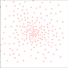 |
Fig. 1. Example of a dynamic grid with 199 points used for the smooth dark matter distribution. |
3. Lens model results
The uncertainty in the derived Hubble constant is dominated by the uncertainty in the lens model. In order to capture this uncertainty, we derived a range of models, all of them consistent with the observed set of linear constraints (positions of lensed galaxies and QSO). The observed time delays or relative magnifications, are not included in our set of constraints. In the case of WSLAP+, a major source of uncertainty in the lens model originates in the particular choice of the grid used to describe the smooth component of the mass. The grid configuration is a free variable in WSLAP+. For the number of constraints used in this work, grid configurations with 150–300 points can produce satisfactory results in terms of reproducing the position of lensed galaxies with relatively smooth critical curves. A larger number of grid points results in unstable and unreliable solutions and smaller numbers result in a lack of resolution. The cases presented should capture the expected range of uncertainty.
Another source of variability comes from the starting point of the minimization. It is possible to choose among an infinite number of initial conditions. After each minimization, each solution differs slightly from other solutions obtained with a different seed. We varied both the grid and initial seed to explore the range of valid models.
3.1. Range of lens models
We derived a total of 21 lens models: one with a uniform grid of 16 × 16 points, nine with a dynamical grid of 199 points, six with a different dynamical grid of 248 points, and an additional five models with a different dynamical grid of 299 points. However, only the 20 multiresolution grids were used to compute the estimation of the Hubble constant since the solution obtained with the regular 16 × 16 grid lacks resolution in the central region.
Figure 2 shows the convergence of 10 of the 21 models used, including the initial model obtained with the uniform grid 16 × 16 = 256 grid points. The first number in the legend indicates the number of grid points, while Model1, Model2, and Model3 are different realizations (different initial conditions) for the same grid configuration. Models that are not shown have similar profiles. These profiles are consistent with the ones derived by Liu et al. (2023) using a parametric model. Despite the relative similarity between profiles, the small changes between models are the main source of uncertainty in the predicted time delay, and hence in the derived value for the Hubble constant. Figure 3 shows the magnification map of the lens model, obtained with the dynamic grid of 199 points in Fig. 1 plotted in red on top of the galaxy cluster shown in blue.
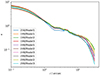 |
Fig. 2. Convergence κ for 10 models computed for a source at z = 1. |
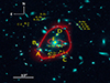 |
Fig. 3. Magnification map of the reconstructed lens of SDSS J1004+4112 using the dynamic grid with 199 points. |
3.2. Predicted time-delay for image E
Each of the lens models described in the previous subsection gives a prediction for the image E time-delay for a canonical Hubble constant H0 = 70 km s−1 Mpc−1. Thus, by re-scaling the predicted time delays to the value of the Hubble constant measured, H0 = 74 km s−1 Mpc−1 (see Sect. 5), we can obtain a predicted time-delay with respect to image C of 3200 ± 200 days. This is approximately 1 yr longer than the expected value reported in Forés-Toribio et al. (2022), who obtained a predicted time delay of about 8 yr.
A robust determination of the time delay of image E (with respect to image C) would play an important role since this measurement would significantly improve the precision in the estimation of the Hubble constant. However, image E is very faint. This means that the typical magnification ratio between images D and E is μD/μE ∼ 30 (with a great variation among different models) and, consequently, it is reasonable to assume that image E is about 30 times fainter than image D at optical wavelengths (neglecting possible extinction and microlensing effects). Hence, if the r-band magnitude of D is ∼21 (see Table 1 of Muñoz et al. 2022), the expected r-band magnitude of D would be ∼24.7 mag. Additionally, E is located in a bright and crowded sky region, so it seems extremely difficult to build its optical light curve from current facilities.
4. Constraints on H0
It is common to express the Hubble constant H0 as:
where h = H0/100 is referred to as the reduced Hubble constant and it is a dimensionless physical constant.
In order to measure H0, Refsdal (1964) proposed that the gravitational lensing effect could be used. In fact, when a light ray is deflected by a gravitational lens, its trajectory is modified and therefore its traveling time, due to the light’s finite propagation speed. The expression that describes the time delay of the perturbed ray with respect to the one that follows a straight path is displayed in Eq. (6):
![Mathematical equation: $$ \begin{aligned} t(\boldsymbol{\theta }) =\frac{1+z_l}{c}\frac{D_lD_s}{D_{ls}}\left[\frac{1}{2}(\boldsymbol{\theta }-\boldsymbol{\beta })^2-\Phi (\boldsymbol{\theta })\right], \end{aligned} $$](/articles/aa/full_html/2024/02/aa48066-23/aa48066-23-eq9.gif) (6)
(6)
with zl indicating the redshift of the lens.
The three angular distances involved in Eq. (6) are inversely proportional to the Hubble constant, H0, therefore, we say that the time delay scales as 1/h. In addition, the magnitude expressed in Eq. (6) is not measurable; instead, we chose to measure the time delay relative to one of the images.
Using the lens models derived in the previous section, we are able to confront the predictions of the time delay of the multiple images of the QSO with the observations, both relative to image C. Our lens models predict the time delay for a canonical value of H0 = 70 km s−1 Mpc−1, which is a reduced Hubble constant of h = 0.7. Hence, these time delays are re-scaled to a new reduced Hubble constant (h′) by multiplying the predicted time delays, x = h′/0.7
4.1. Likelihood
For each lens model, we can derive a probability for the presence of h by minimizing the weighted difference between the predicted and observed time delays (ΔTMi and ΔTobs, respectively):
![Mathematical equation: $$ \begin{aligned} p(M_i,h) \propto \prod _{j=\mathrm{A,B,C,D}} \exp \left[-\frac{(\Delta T_{M_i}^j-\Delta T_{\rm obs}^j)^2}{2\sigma _j^2} \right], \end{aligned} $$](/articles/aa/full_html/2024/02/aa48066-23/aa48066-23-eq10.gif) (7)
(7)
where the index j runs over the four positions, A, B, C, and D. In addition, the proportionality sign just expresses the lack of a normalization constant. The values of σj are computed at each of these four positions as the dispersions of the time delays predicted by the lens models. Image E has no observable time delay and hence is not included in the definition of the likelihood.
Since we have different lens models derived under different assumptions, we need to compute the joint probability from all models. We adopted the conservative approach that the combined probability from all lens models is the sum of probabilities of the models (see, e.g., Vega-Ferrero et al. 2018). A more aggressive approach would be to consider that the joint probability is the product of the individual probabilities, but this implies all models are independent from each other. This is not true since all lens models are derived using the same algorithm, with some assumptions common to several models (e.g., the grid configuration, definition of the compact component, or lensing constraints).
The joint probability is then defined as:
 (8)
(8)
where the sum runs over the N lens models, p(Mi, h) is the probability given in Eq. (7) and the term wi is the weight assigned to each model. Once again, the proportionality sign just indicates the lack of a normalization constant. This weight is determined by how well a particular model reproduces the observed flux ratios between the different images of the QSO. We define this weight as (dropping the subscript i);
![Mathematical equation: $$ \begin{aligned} w = \exp \left[-\frac{1}{2}\left(\frac{(\frac{F_{\rm B}}{F_{\rm C}}-\frac{\mu _{\rm B}}{\mu _{\rm C}})^2}{\sigma _{\mathrm{CB}}^2} \right.\right. + \left.\left.\frac{(\frac{F_{\rm D}}{F_{\rm C}}-\frac{\mu _{\rm D}}{\mu _{\rm C}})^2}{\sigma _{\mathrm{CD}}^2}\right)\right]\cdot \end{aligned} $$](/articles/aa/full_html/2024/02/aa48066-23/aa48066-23-eq12.gif) (9)
(9)
In the above definition, we have ignored image E since this is very close to the center of the BCG galaxy and extremely faint. In addition, initially, we did not include the flux ratio, FA/FC, in w Eq. (9) because the A image is very close to a critical line and, thus, the magnification ratio, μA/μC, in some models might be a strongly biased estimator of FA/FC. Hence, in an abundance of caution, image A was ignored for respect to the definition of the weight. We computed the flux ratios as the average of three flux ratios from our own measurements in the IR band F814W, measurements published in Oguri (2010) and radio flux in Hartley et al. (2021). The values of σCB, and σCD are the combination of the observed dispersion of flux ratios between different measurements and the expected variation due to the intrinsic variability:
 (10)
(10)
For the intrinsic variability in the F814W HST filter, we adopted a value of σint = 0.2 for image B and σint = 0.16 for image D from Li et al. (2018) and Morganson et al. (2014). The measured time delays, flux ratios measured by the indicated authors, and estimated intrinsic variability are summarized in Table 1. The flux ratios from Oguri and this work correspond to the F814W HST filter and Hartley’s in the 5 GHz radio band.
Observed time delay, flux ratios, and adopted intrinsic flux ratio variation for the QSO images of SDSS J1004.
5. H0 results
Each of the models obtained in this work has a different contribution to the prediction of the value of the Hubble constant. Figure 4 shows the contribution of each of the models to the final likelihood, this is, it shows the function defined by each weighted probability in the likelihood function in Eq. (8).
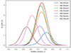 |
Fig. 4. Contribution of the seven models with the highest weights to the final likelihood. |
Our main results are incorporated in Fig. 5. In this figure, we show the probability for the reduced Hubble constant using three different schemes. The standard scheme relies on Eqs. (7)–(9) and the 20 lens models, leading to the probability distribution shown in blue. Selecting the 11 lens models with the highest resolutions (248 and 299 grid points), we were also able to obtain the distribution in red. Additionally, we considered the 20 lens models and a modified version of Eq. (9), including flux ratios with respect to A (flux ratios FB/FA, FC/FA, and FD/FA) and the corresponding model magnification ratios, to produce the probability distribution in green. The shaded regions outline the 68% confidence intervals. Thus,
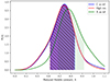 |
Fig. 5. Probability distribution of h obtained from time-delay predicted by the lens models using different analyses. |
6. Conclusions
These results are in agreement with recent estimates reported in Liu et al. (2023) and Napier et al. (2023). The present paper, along with these two works, show that the Hubble constant must lie in the 60 − 80 km s−1 Mpc−1 range. The uncertainty in H0 can be reduced in the future with deeper observations of this cluster, which would reveal more lensed galaxies and their corresponding redshifts. This would take advantage of lensing by galaxy clusters, which typically can have over an order of magnitude more lensing constraints than classic galaxy-QSO lensing. Also, future observations of lensed SNe in galaxy clusters will provide competitive constraints on H0, similar to those obtained with SN Refsdal (Vega-Ferrero et al. 2018; Kelly et al. 2023), or SN H0pe (Frye, in prep.).
To conclude, we analyze the contribution of this work to the Hubble tension problem. The Hubble tension refers to the 4σ to 6σ discrepancy between estimations of H0 from early universe measurements and late universe results. The most precise predictions of the Hubble constant using early universe results come from the CMB Plank Collaboration (Planck Collaboration XII 2020) that obtained H0 = 67.49 ± 0.53 km s−1 Mpc−1 with 68% confidence level (CL). In the late universe, however, the most precise results come from different techniques: using distance ladder Cepheid calibration in the Large Magellanic, Riess et al. (2019) estimated H0 = 74.03 ± 1.42 km s−1 Mpc−1; the SNe Ia distance calibration by the SH0ES collaboration (Riess et al. 2022) that obtained H0 = 73.30 ± 1.04 km s−1 Mpc−1 (68% CL); and gravitational lensing on quasars by H0LiCOW collaboration (Wong et al. 2019) that obtained  km s−1 Mpc−1 (68% CL) and TDCOSMO with
  km s−1 Mpc−1 (Shajib et al. 2023) in their latest result. There is a chance that the tension might be fictitious (e.g., the resulting effects of the selection of the SNe Ia or use of inadequate lens mass models) or real, in which case a modified cosmological model would be required (e.g., Dainotti et al. 2021; Goicoechea & Shalyapin 2023; Shalyapin et al. 2023). Nonetheless, our results do not show any tension with any of the results in either the early universe or late universe, although this is largely due to the lens model uncertainties.
Acknowledgments
We thank Dominique Sluse for his valuable comments and suggestions that allowed us to correct and improve this manuscript. As an answer to one of his suggestions, we incorporated Table A.1 in the Appendix in the current paper, as these can be useful in microlensing studies. In addition, Luis J. Goicoechea acknowledges the support from the grant PID2020-118990GB-I00 funded by MCIN/AEI/10.13039/501100011033.
References
- Dainotti, M. G., De Simone, B., Schiavone, T., et al. 2021, ApJ, 912, 150 [NASA ADS] [CrossRef] [Google Scholar]
- Diego, J. M., Protopapas, P., Sandvik, H. B., & Tegmark, M. 2005, MNRAS, 360, 477 [Google Scholar]
- Diego, J. M., Tegmark, M., Protopapas, P., & Sandvik, H. B. 2007, MNRAS, 375, 958 [NASA ADS] [CrossRef] [Google Scholar]
- Fohlmeister, J., Kochanek, C., Falco, E., et al. 2007, ApJ, 662, 62 [NASA ADS] [CrossRef] [Google Scholar]
- Fohlmeister, J., Kochanek, C., Falco, E., Morgan, C., & Wambsganss, J. 2008, ApJ, 676, 761 [NASA ADS] [CrossRef] [Google Scholar]
- Forés-Toribio, R., Muñoz, J. A., Kochanek, C. S., & Mediavilla, E. 2022, ApJ, 937, 35 [CrossRef] [Google Scholar]
- Goicoechea, L. J., & Shalyapin, V. N. 2023, in The Sixteenth Marcel Grossmann Meeting. On Recent Developments in Theoretical and Experimental General Relativity, Astrophysics, and Relativistic Field Theories, eds. R. Ruffini, & G. Vereshchagin (World Scientific Publishing Co. Pte. Ltd.), 1990 [Google Scholar]
- Hartley, P., Jackson, N., Badole, S., et al. 2021, MNRAS, 508, 4625 [NASA ADS] [CrossRef] [Google Scholar]
- Inada, N., Oguri, M., Pindor, B., et al. 2003, Nature, 426, 810 [NASA ADS] [CrossRef] [Google Scholar]
- Inada, N., Oguri, M., Morokuma, T., et al. 2006, ApJ, 653, L97 [Google Scholar]
- Kelly, P. L., Rodney, S., Treu, T., et al. 2023, Science, 380, abh1322 [NASA ADS] [CrossRef] [Google Scholar]
- Li, Z., McGreer, I. D., Wu, X.-B., Fan, X., & Yang, Q. 2018, ApJ, 861, 6 [NASA ADS] [CrossRef] [Google Scholar]
- Liesenborgs, J., De Rijcke, S., Dejonghe, H., & Bekaert, P. 2009, MNRAS, 397, 341 [NASA ADS] [CrossRef] [Google Scholar]
- Liu, Y., Oguri, M., & Cao, S. 2023, Phys. Rev. D, 108, 083532 [Google Scholar]
- Meneghetti, M., Natarajan, P., Coe, D., et al. 2017, MNRAS, 472, 3177 [Google Scholar]
- Mohammed, I., Saha, P., & Liesenborgs, J. 2015, PASJ, 67, 21 [NASA ADS] [CrossRef] [Google Scholar]
- Morganson, E., Burgett, W. S., Chambers, K. C., et al. 2014, ApJ, 784, 92 [NASA ADS] [CrossRef] [Google Scholar]
- Muñoz, J., Kochanek, C., Fohlmeister, J., et al. 2022, ApJ, 937, 34 [CrossRef] [Google Scholar]
- Naohisa, I., Oguri, M., Keeton, C. R., et al. 2005, PASJ, 57, L7 [Google Scholar]
- Napier, K., Sharon, K., Dahle, H., et al. 2023, Am. Astron. Soc. Meet. Abstr., 55, 130.02 [NASA ADS] [Google Scholar]
- Oguri, M. 2010, PASJ, 62, 1017 [NASA ADS] [Google Scholar]
- Oguri, M., Inada, N., Keeton, C. R., et al. 2004, ApJ, 605, 78 [NASA ADS] [CrossRef] [Google Scholar]
- Perera, D., Williams, L. L. R., Liesenborgs, J., Ghosh, A., & Saha, P. 2024, MNRAS, 527, 2639 [Google Scholar]
- Planck Collaboration XII. 2020, A&A, 641, A12 [NASA ADS] [CrossRef] [EDP Sciences] [Google Scholar]
- Press, W., Teukolsky, S., Vetterling, W., & Flannery, B. 1997, Numerical Recipes in Fortran 77 (Cambridge University Press) [Google Scholar]
- Refsdal, S. 1964, MNRAS, 128, 307 [NASA ADS] [CrossRef] [Google Scholar]
- Riess, A. G., Casertano, S., Yuan, W., Macri, L. M., & Scolnic, D. 2019, ApJ, 876, 85 [Google Scholar]
- Riess, A. G., Yuan, W., Macri, L. M., et al. 2022, ApJ, 934, L7 [NASA ADS] [CrossRef] [Google Scholar]
- Saha, P., Read, J. I., & Williams, L. L. R. 2006, ApJ, 652, L5 [NASA ADS] [CrossRef] [Google Scholar]
- Shajib, A. J., Mozumdar, P., Chen, G. C.-F., et al. 2023, A&A, 673, A9 [NASA ADS] [CrossRef] [EDP Sciences] [Google Scholar]
- Shalyapin, V. N., Goicoechea, L. J., Dyrland, K., & Dahle, H. 2023, ApJ, 955, 140 [NASA ADS] [CrossRef] [Google Scholar]
- Sharon, K., Ofek, E. O., Smith, G. P., et al. 2005, ApJ, 629, L73 [NASA ADS] [CrossRef] [Google Scholar]
- Vega-Ferrero, J., Diego, J. M., Miranda, V., & Bernstein, G. M. 2018, ApJ, 853, L31 [NASA ADS] [CrossRef] [Google Scholar]
- Williams, L. L., & Saha, P. 2004, AJ, 128, 2631 [NASA ADS] [CrossRef] [Google Scholar]
- Wong, K. C., Suyu, S. H., Chen, G. C.-F., et al. 2019, MNRAS, 498, 1420 [Google Scholar]
Appendix A: Additional estimated parameters
Table A.1 includes the convergence, κ; shear, γ; and shear direction, ϕ, for the quasar’s five images for the 20 lens models used in this work for the estimation of the Hubble constant, together with the mean value for these in the last row of the Table.
Convergence κ, shear γ and shear direction ϕ of the multi-resolution lens models for the different QSO images.
All Tables
Observed time delay, flux ratios, and adopted intrinsic flux ratio variation for the QSO images of SDSS J1004.
Convergence κ, shear γ and shear direction ϕ of the multi-resolution lens models for the different QSO images.
All Figures
|
Fig. 1. Example of a dynamic grid with 199 points used for the smooth dark matter distribution. |
| In the text | |
|
Fig. 2. Convergence κ for 10 models computed for a source at z = 1. |
| In the text | |
|
Fig. 3. Magnification map of the reconstructed lens of SDSS J1004+4112 using the dynamic grid with 199 points. |
| In the text | |
|
Fig. 4. Contribution of the seven models with the highest weights to the final likelihood. |
| In the text | |
|
Fig. 5. Probability distribution of h obtained from time-delay predicted by the lens models using different analyses. |
| In the text | |
Current usage metrics show cumulative count of Article Views (full-text article views including HTML views, PDF and ePub downloads, according to the available data) and Abstracts Views on Vision4Press platform.
Data correspond to usage on the plateform after 2015. The current usage metrics is available 48-96 hours after online publication and is updated daily on week days.
Initial download of the metrics may take a while.