| Issue |
A&A
Volume 645, January 2021
|
|
|---|---|---|
| Article Number | A44 | |
| Number of page(s) | 15 | |
| Section | Cosmology (including clusters of galaxies) | |
| DOI | https://doi.org/10.1051/0004-6361/202038248 | |
| Published online | 07 January 2021 | |
Cosmology with gravitationally lensed repeating fast radio bursts
1
Max-Planck-Institut für Radioastronomie, Auf dem Hügel 69, 53121 Bonn, Germany
e-mail: This email address is being protected from spambots. You need JavaScript enabled to view it.
2
Canadian Institute for Theoretical Astrophysics, University of Toronto, 60 St. George Street, Toronto, Ontario M5S 3H8, Canada
3
Dunlap Institute for Astronomy and Astrophysics, University of Toronto, 50 St. George Street, Toronto, Ontario M5S 3H4, Canada
4
Canadian Institute for Advanced Research, CIFAR Program in Gravitation and Cosmology, 661 University Ave, Toronto, Ontario M5G 1Z8, Canada
5
Perimeter Institute for Theoretical Physics, 31 Caroline Street North, Waterloo, Ontario N2L 2Y5, Canada
Received:
24
April
2020
Accepted:
16
October
2020
Abstract
High-precision cosmological probes have revealed a small but significant tension between the parameters measured with different techniques, among which there is one based on time delays in gravitational lenses. We discuss a new way of using time delays for cosmology, taking advantage of the extreme precision expected for lensed fast radio bursts, which are short flashes of radio emission originating at cosmological distances. With coherent methods, the achievable precision is sufficient for measuring how time delays change over the months and years, which can also be interpreted as differential redshifts between the images. It turns out that uncertainties arising from the unknown mass distribution of gravitational lenses can be eliminated by combining time delays with their time derivatives. Other effects, most importantly relative proper motions, can be measured accurately and disentangled from the cosmological effects. With a mock sample of simulated lenses, we show that it may be possible to attain strong constraints on cosmological parameters. Finally, the lensed images can be used as galactic interferometer to resolve structures and motions of the burst sources with incredibly high resolution and help reveal their physical nature, which is currently unknown.
Key words: gravitational lensing: strong / distance scale
© O. Wucknitz et al. 2021
 Open Access article, published by EDP Sciences, under the terms of the Creative Commons Attribution License (https://creativecommons.org/licenses/by/4.0), which permits unrestricted use, distribution, and reproduction in any medium, provided the original work is properly cited.
Open Access funding provided by Max Planck Society.
1. Introduction
The gravitational lens effect (Refsdal 1964a) can deflect light so strongly that it produces multiple images of a single source. Refsdal (1964b) argued that time delays (light travel time differences between images) can be used to determine distances and, thus, the Hubble constant (H0), at a time when it was not even clear that the effect would ever be seen in observations. For very distant systems, Refsdal (1966) showed that time delays can also be used to test cosmological theories.
The practical applications of this brilliantly simple idea turned out to be quite difficult. Even after the discovery of the first gravitationally lensed active galactic nucleus (AGN) by Walsh et al. (1979), it took many years before the time delay between the two images was agreed upon with sufficient accuracy. The main reasons for this difficulty come from the typically slow intrinsic variations of AGN as compared to the lensed supernovae that were originally proposed.
An even more fundamental difficulty is the influence of the a priori unknown mass distribution of the lens on the derived results. Parameterised mass models can often be fitted to the observed image configuration, flux ratios, and relative image distortions. In the best case, extended sources with rich substructures provide a wealth of constraints for realistic multi-parameter mass distributions. However, there are fundamental degeneracies between the lensing mass distribution and the unknown intrinsic source structure.
Best-known is the mass-sheet degeneracy (Falco et al. 1985; Gorenstein et al. 1988), according to which scaling a given mass distribution while adding a homogeneous mass sheet can leave the image configuration unchanged, provided that the source structure and position is scaled accordingly. This transformation also scales the time delay and thus the derived Hubble constant. More realistic, but very similar in effect, are changes of the radial mass profile of the lens. A more general degeneracy has been described by Schneider & Sluse (2014).
Additional measurements of the velocity dispersion of lensing galaxies can partly break these degeneracies, but at the cost of introducing additional complex astrophysics into the problem. Nevertheless, very competitive results have been achieved so far. Wong et al. (2019) describe results from a joint analysis of six gravitational lenses. Their result for the Hubble constant is precise to 2.4%, but disagrees with cosmic microwave background (CMB) results far beyond the formal uncertainties (Planck Collaboration VI 2020). Millon et al. (2020b) discuss systematic uncertainties in the lensing analysis. Kochanek (2020) presents a more pessimistic view and argues that accuracies below 10% are hardly possible, regardless of the formal precision.
Even though the tension between determinations of the Hubble constant with different methods is well below 10% at present, it is still highly significant. These differences may result from a limited understanding of the systematics involved or, for instance, a certain behaviour exhibited by dark energy that is different than that assumed based on simple models. Either way, there is a need for additional clean methods with preferably less (or, at least, different) systematics. In this work, we argue that a novel application of gravitational lensing is a very promising option. The unique properties of fast radio bursts (FRBs) are essential for this approach, which diverges from related ideas presented in the literature. For example, Li et al. (2018) and Liu et al. (2019) propose using the high accuracy of time delays measured from gravitationally lensed FRBs together with classical mass modelling. They argue that the absence of a bright AGN core in FRB host galaxies facilitates the use of optical substructures as lens modelling constraints.
This essential new observable – namely, time delay changes over time – has been discussed by Piattella & Giani (2017) for rather special lenses. Zitrin & Eichler (2018) explicitly investigate the fact that time derivatives of time delays (as expected from cosmic expansion) may be measurable with lensed FRBs. They also discuss the notion that the relative proper motion of the source has a strong effect that is difficult to distinguish from cosmological expansion.
Here, we argue that with coherent time-delay measurements, we can achieve levels of accuracy that are much better than the burst duration and not only does this allow us to disentangle cosmological effects from the proper motion, but we can even eliminate the unknown mass distributions of the lensing galaxies as the main source of potential systematic errors.
This manuscript is structured as follows. In Sect. 2, we describe the sources (FRBs) that can be used to determine time delays at a level of precision that even allows us to measure how they evolve over time. In Sect. 3, we describe how these new observables can be used to avoid the effects of the unknown mass distribution almost entirely. It turns out that relative transverse motion has a stronger effect than cosmology. We discuss how this effect can be removed, with the additional result of measuring the proper motion with unprecedented accuracy. In Sect. 4, we discuss the level to which we may be able to determine combinations of cosmological parameters based on realistic measurements. We find that with an ensemble of lens systems, we can potentially obtain competitive constraints on a number of parameters.
At the level of precision that is required and achievable, many additional small effects have to be considered. These possible caveats are the subject of Sect. 5. Similar to the proper motion, these are also interesting in themselves. The use of gravitationally lensed images as arms of a galaxy-size interferometer is discussed in Sect. 6. We can potentially resolve structures of a few kilometres at cosmological distances. At the same time, the required time-delay precision is only achievable for sources that actually have structures on these scales, which is only true for fast radio bursts. A discussion and summary is presented in Sect. 7.
2. Fast radio bursts (FRBs)
A new type of radio sources was discovered by Lorimer et al. (2007), which are bright radio bursts with durations of less than a few milliseconds. Similarly to pulsars, their signals are dispersed; they arrive later at lower frequencies. In FRBs, this dispersion is higher than expected from the integrated electron column density within the Milky Way, which is evidence for an extragalactic origin at cosmological distances. The first of these objects were detected only once, which makes an accurate localisation difficult. The discovery of the first repeating FRB by Spitler et al. (2016) changed the game completely. Observing the roughly known location with the Karl G. Jansky Very Large Array (VLA) allowed Chatterjee et al. (2017) to localise it to sub-arcsecond accuracy. This was sufficient to identify a host galaxy and thus determine the redshift z = 0.1927 of the host and FRB (Tendulkar et al. 2017). This comprised the final proof that (at least) this FRB originates at a cosmological distance. Marcote et al. (2017) determined the position to milli-arcsec (mas) accuracy with Very Long Baseline Interferometry (VLBI).
The first direct localisation at discovery of another FRB source was achieved with the Australian Square Kilometre Array Pathfinder (ASKAP) by Bannister et al. (2019), which led to the identification of a host galaxy at z = 0.3214. The same instrument is now finding new FRBs regularly. An even higher yield is produced by the Canadian HI Intensity Mapping Experiment (CHIME, CHIME/FRB Collaboration 2018), which does now find several new FRBs per day. CHIME also discovered the second repeating FRB (CHIME/FRB Collaboration 2019), so far without an accurate localisation. The first VLBI-localisation of another repeater found by CHIME was presented by Marcote et al. (2020).
Given that these instruments, even though they are considered wide-field, can only observe a small fraction of the sky, the number of FRBs that are detectable by a true all-sky survey with sensitivities comparable to current facilities must at least be hundreds, if not thousands per day. At the same time, radio astronomical technology is making rapid progress, which makes a full-sky FRB monitoring feasible in the foreseeable future.
Currently, the redshift distribution can only be estimated, which makes it difficult to predict the fraction that is gravitationally lensed. The Cosmic Lens All Sky Survey (CLASS, Browne et al. 2003) found that one out of 700 of their AGN source population is strongly lensed, with multiple images on arcsecond scales. Marlow et al. (2000) studied the redshift distribution of the CLASS parent source population and found a wide range with a mean of z = 1.2 and a root mean square (rms) scatter of 0.95. The known source redshifts from Browne et al. (2003) are 0.96, 1.013, 1.28, 1.34, 1.39, 2.62, 3.214, and 3.62. Even though the FRB population may be systematically closer to us, which reduces the chance of gravitational lensing, the future discovery of lensed FRBs is a realistic possibility. Some fraction of them will be repeating, which will allow us to measure how time delays evolve over time and to apply the approach presented in this work. We note that we have to distinguish between the concepts of bursting FRB sources, individual bursts from FRB sources, and lensed “echoes” (or images) of individual bursts.
With lensed bursts of millisecond durations, it is obvious that time delays can be measured with at least this level of accuracy. Typical time delays are on the order of days to months, and for order-of-magnitude estimates, we assume 106 s, that is, approximately 12 days; see Table 1 for the numbers that we use for our estimates. The fractional accuracy is then 10−9, a huge leap forward compared to the few-percent level that is (at the utmost) achievable with lensed AGN. Millon et al. (2020a) present a table of known and new time delays of quasars lensed by single galaxies. Uncertainties are mostly above one day. A particularly good time delay for B0218+357 is known from gamma-ray observations (Cheung et al. 2014) and radio monitoring (Biggs & Browne 2018). The results are consistent with each other and have uncertainties of 0.16 and 0.2 days, respectively. Significant improvement beyond this is not expected for lensed AGN.
Typical order-of-magnitude values referred to in the text.
As Li et al. (2018) argue, the uncertainty of the time delay measurements for lensed FRBs is entirely negligible in the total error budget. Because the lensed host galaxies of FRBs are generally not expected to harbour a strong AGN, their structure in optical images may make lens modelling more accurate as well, so that a level of 1% might be reachable with ten lensed FRBs (Li et al. 2018). We do have some concerns that even if this approach might certainly reduce some uncertainties, the fundamental mass-model degeneracies persist and could lead to significant systematic errors even in a joint analysis of many lenses. For this reason, we propose an alternative route for cosmology with lensed FRBs.
We need an even higher accuracy of the time delays to follow this route. Fortunately, this is made possible by lensed FRBs. If we can observe not only the intensity as function of time, but the full electromagnetic wave field from a source, and if we have two coherent copies of the wave field from the same burst, then we can determine the time delay (group delay) between them with an uncertainty given by the reciprocal bandwidth. With good signal-to-noise ratio (S/N), the accuracy can be improved even more. Modern radio receivers have bandwidths of hundreds of MHz up to a few GHz, so that uncertainties smaller than a nanosecond are certainly achievable. In principle, we may even use the (absolute) phase delay, with uncertainties given by the reciprocal observing frequency1. In reality, practical problems like clock drifts as well as ionospheric and atmospheric delays have to be considered. We show below that as result of time-varying time delays, different images will have different redshifts. For short bursts, this effect is so small that it generally does not have to be taken into account in the correlation analysis, but can easily be included when needed. What has to be included, on the other hand, are differences of dispersion in the interstellar medium of the lensing galaxy that produce frequency-dependent delay differences. These follow a λ2 law and can be corrected with a coherent de-dispersion.
Achieving nanosecond accuracy over time ranges of weeks and months is not entirely unrealistic, but we base our arguments on a much more conservative assumption of uncertainty, namely at the level of one microsecond (Table 1), which corresponds to a fractional uncertainty of the typical time delay on the order of 10−12. We note that this coherent way of measuring time delays does not rely on short bursts, or even on the presence of intrinsic intensity variations, because it uses the wave field itself. It is, however, essential that the images are mutually coherent, which is not the case for any sources other than FRBs, as explained in Sect. 6. Of course finding the time delay between the waves is made much easier when we have a good estimate from the intensity correlation.
3. Theory
3.1. Homogeneously expanding Universe
Our general idea is very simple: As result of the expansion of the Universe, time delays should also roughly increase at this rate, dΔt/dt ∼ H0 Δt, which over about three years (Table 1) corresponds to a change of 0.2 ms or a fractional change of 2 × 10⁻¹⁰, which is easily measurable with an accuracy of better than one percent. In the following, we derive how this time-delay increase is related to cosmological parameters and observables.
For the moment, we assume that the entire Universe, including the gravitational lens, expands uniformly with a geometry according to the following metric2:
 (1)
(1)
 (2)
(2)
 (3)
(3)
 (4)
(4)
Here t denotes cosmic time (also proper time of comoving observers), R(t) is the scale factor, and dL is the comoving length interval. The comoving spatial coordinates are xj and the spatial metric, γij, does not depend on time.
Under this condition, light rays follow spatial geodesics with a time-dependence defined by the speed of light. Light rays connecting the comoving source and the observer at different times follow the same spatial path and are shifted by a constant interval in the conformal time coordinate, η, which provides the important relation between scale factor and redshift,
 (5)
(5)
In the case of a gravitational lens, the time delay will not vary over time if measured in terms of η. Because the measured time delay, Δt, is a scaled version of Δη, its logarithmic time-derivative is a direct measurement of the current Hubble constant:
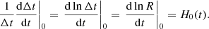 (6)
(6)
In this unrealistic situation, the time delay increases exactly in proportion with the expanding Universe. We could thus measure the Hubble constant directly, without mass model uncertainties and even without knowing image positions or redshifts. In reality the gravitational lens itself does not expand with the Hubble flow and we have to derive the effect in detail as shown in the following.
3.2. Lensing theory
With the image position θ, the true source position θs and the apparent deflection angle α, the lens equation reads
 (7)
(7)
where all angles are small two-dimensional vectors in the tangential plane relative to some reference axis.
Time delays can be derived using the methods described by Cooke & Kantowski (1975). For this, we do not need to assume a certain cosmological model as long as we parameterise it by angular size distances between observer and lens Dd, between observer and source Ds, and between lens and source Dds. Here, we use the subscripts d and s for deflector and source, respectively, and suppressed 0 for the current epoch (observer). We assume that the global geometry of the Universe still follows the homogeneous expansion according to Eqs. (1)–(4). Later in this paper, we include the effect of radial motion into these parameters.
An angular size distance, Dab, is defined as the ratio between a transverse offset at b and the corresponding angle measured at a, where both sides are considered at the cosmic time at which the signal passes. Because the spatial geodesics do not change in comoving coordinates and because the length is measured at b, this distance scales with Rb over time, as long as a and b are fixed in comoving coordinates. We later relax the assumption that light rays follow geodesics of the average global spacetime and allow for systematic overdensities (or underdensitites) near the light path.
The time delay measured by an observer consists of a geometric component and the Shapiro (or potential) component3,
![Mathematical equation: $$ \begin{aligned}&c\,\Delta t_0 = {D_{\rm eff}^\prime} \left[ \frac{(\boldsymbol{\theta }-\boldsymbol{\theta }_{\rm s})^2}{2} - \psi (\boldsymbol{\theta }) + \mathrm{const.} \right] {,} \end{aligned} $$](/articles/aa/full_html/2021/01/aa38248-20/aa38248-20-eq8.gif) (8)
(8)
 (9)
(9)
Later on, we absorb the  term into the constant.
The Shapiro delay is described via the lensing potential ψ, which is related to the delay, τd, as measured in the lens frame via
 (10)
(10)
The lens Eq. (7) results from Fermat’s principle with α = ∇θψ.
3.3. Lensing-induced redshifts
The time delay will slowly change over time in a way that is more complicated than in the relatively the naive equation in Eq. (6). Details are presented in the following.
The time derivative of the time delay can also be interpreted as additional lensing-induced redshift z(θ), in the sense that the time lag between subsequent bursts in image θ scales with 1 + z(θ). This scaling only has a meaning as relative redshift between images, z(θ1) − z(θ2), similar to the time delay itself, which only has a unique definition as delay between images.
The lag between bursts (in contrast to the delay between lensed images of the same burst) cannot be measured coherently and, therefore, has a much lower accuracy on the order of a millisecond. Because we measure the redshift as the difference of time derivatives of time delays, which are measured coherently, the achievable accuracy is actually given by the ratio of the coherent timing uncertainty and the burst separation. If we use Latin letters as indices for images and Arabic numbers for the bursts (dropping the subscript 0 in t0), the relation can be written as:
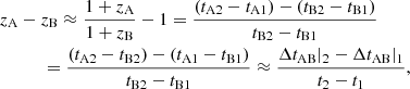 (11)
(11)
which is correct to the first order in z and thus sufficient for all practical purposes. For real measurements, we can use as many bursts as available and fit them jointly.
Based on the values in Table 1, the measurement accuracy in z is on the order of 10−14 even under our conservative assumptions. This is better than for the relative change of the time delay because the relevant baseline is the time between bursts, which can be many years, and which increases without limit if the FRB is repeating persistently. It is this extreme precision that makes gravitationally lensed FRBs such a promising tool. Because we want to measure a tiny effect (time-delay increase due to the expanding Universe) with extreme precision, we have to consider many other effects that may influence the results. In the analysis below we find no show-stoppers, but some of the additional effects (most importantly the proper motion) are interesting even in themselves.
3.4. Distance parameters in a Robertson-Walker Universe
For most of the final analysis, we assume that the general geometry (with the exception of the lens) is expanding homogeneously according to Eqs. (1) and (4). This means that the angular size distance, Dab, can be written as a comoving (and thus constant) angular size distance multiplied with the scale factor, Rb. This is a common assumption in lensing theory, but at the level of accuracy that is required to understand the current tension in cosmological parameters, this simplification may no longer be sufficient.
World models that are homogeneous on large scales, but have small-scale deviations near the light paths, have been introduced by Kantowski (1969), Dyer & Roeder (1972) and Dyer & Roeder (1973). The basic idea is that matter is clumped, but clumps near the line of sight are explicitly described as gravitational lenses, so that the remaining density around the light rays may be reduced relative to the global mean, which reduces the focusing and increases the angular size distances. These inhomogeneities can also be described explicitly as perturbations at certain redshifts along the line of sight. Even if we can describe the effect well (e.g. if the inhomogeneity parameter in the Dyer-Roeder distance is known), they break the symmetry of the homogeneously expanding geometry.
In the following derivations, we typically start with the general case (described by angular size distances and their derivatives) before we consider the homogeneous case, in which the time-derivatives of distance parameters and the prefactor in Eq. (8) can be derived as follows, using variants of Eq. (6):
 (12)
(12)
 (13)
(13)
 (14)
(14)
In the scenario in which the geometry of the entire Universe, including the lens, expands homogeneously, the potential and, thus, the image positions do not change, so that Eq. (14) describes the only variation with time in Eq. (8). This confirms our general result from Eq. (6).
We note that the relation
 (15)
(15)
always holds, even in the inhomogeneous case.
3.5. Non-expanding lens
We write the Shapiro delay in Eq. (10) in terms of a physical vector, x = Ddθ and assume that the function τd(x) is invariant as result of the invariant mass distribution in physical space. By writing the equation twice, once for a reference epoch (superscript ref) and once in general but for the same argument of τd, we can derive how the lensing potential ψ of a constant physical mass distribution varies over time:
 (16)
(16)
 (17)
(17)
The resulting deflection angle scales such that
 (18)
(18)
 (19)
(19)
The last form is designated for homogeneous expansion and means that it is invariant for fixed physical vector, x, which is exactly what we expect for an invariant physical mass distribution. This relation automatically holds for an isothermal lens, in which the deflection angle does not vary in the radial direction. Therefore, such a mass distribution produces time delays growing with H0, but this behaviour can only be utilised if we know that the lens is isothermal. In that situation, we do not need the relative redshifts at all, but we can determine the Hubble constant directly from the time delays, for instance, by using the formalism presented by Wucknitz (2002).
For the time derivative of Eq. (8), we can neglect the resulting shift of image positions because they do not affect the light travel time as result of Fermat’s principle. For the time-derivative of the potential at fixed θ, we have to consider both scalings in Eq. (16) and remember that the gradient is the deflection angle:
 (20)
(20)
 (21)
(21)
![Mathematical equation: $$ \begin{aligned}&\qquad \ \ = \frac{H_{\rm d}}{1+z_{\rm d}} \, \Bigl [ (\boldsymbol{\theta }-\boldsymbol{\theta }_{\rm s})\cdot \boldsymbol{\theta }- \psi (\boldsymbol{\theta }) \Bigr ]{.} \end{aligned} $$](/articles/aa/full_html/2021/01/aa38248-20/aa38248-20-eq23.gif) (22)
(22)
The last equation is designated for the homogeneous Universe.
3.6. Transverse motion
It has been known for years that the transverse motion of a gravitational lens relative to the optical axis has an effect on the observed redshifts of lensed images. This effect can be interpreted in different ways; for instance, as a Doppler effect (Birkinshaw & Gull 1983), gravitomagnetic effect of the moving lens (e.g. Pyne & Birkinshaw 1993; Kopeikin & Schäfer 1999), as energy transfer in the scattering of photons by the lens (Wucknitz & Sperhake 2004), or directly as time delays changing with the changing geometry (Zitrin & Eichler 2018).
With transverse velocities, Vs, Vd and V0, of the source, lens, and observer, we can define the proper motions
 (23)
(23)
 (24)
(24)
and write the result of Wucknitz & Sperhake (2004) for the motion-induced redshift as
![Mathematical equation: $$ \begin{aligned} c\, z_{\rm p.m.}(\boldsymbol{\theta }) = \left[ {D_{\rm eff}^\prime} \left( \dot{\boldsymbol{\theta }}_{\rm d}-\dot{\boldsymbol{\theta }}_{\rm s}\right) - \boldsymbol{V}_0\right]\cdot \boldsymbol{\theta }{.} \end{aligned} $$](/articles/aa/full_html/2021/01/aa38248-20/aa38248-20-eq26.gif) (25)
(25)
As a consistency check for the difference between images, we can take the contribution to the time-derivative of Eq. (8) due to the proper motion of the source and confirm that it is consistent with Eq. (25) in the case of a fixed lens and observer. When taking the derivative, we can again neglect the shift of the images because of Fermat’s principle.
For a transverse speed of 300 km s−1, the induced redshift for image separations of 1 arcsec amounts to 5 × 10⁻⁹, corresponding to radial Doppler speeds of 1.5 m s−1. Birkinshaw & Gull (1983) had already suggested measuring this effect on the CMB caused by moving clusters of galaxies, but concluded that it is difficult. Molnar & Birkinshaw (2003) estimated that detecting the effect with optical spectroscopy is challenging even for massive clusters of galaxies. Radio frequencies can be measured with much higher accuracy, but redshifts can only be determined for sufficiently narrow spectral features.
With repeating FRBs, we can eventually measure relative redshifts with a precision on the order of 10−14 and not by measuring the radio frequency, but the time lag between bursts, via coherent measurements of time delays as explained above. This accuracy corresponds to transverse speeds of only about one metre per second or proper motions on the order of 10−13 arcsec per year. Later in this paper, we demonstrate how well the proper motion can be disentangled from the various other effects on the redshifts.
We note that in the equation for the scaling of the lensing potential of a non-expanding lens in Eq. (16), we implicitly assumed that the centre of the scaling law is the coordinate origin. An offset in this centre is equivalent to an additional proper motion that corresponds roughly to the offset over a Hubble time.
3.7. Combining delays and redshifts
We now try to combine the equations for the time delays, Eq. (8), with the ones for its derivatives (or redshifts), including the contribution from the non-expanding lens, Eq. (21), and the transverse motion of the source from Eq. (25). For simplicity, we assume that lens and observer are at rest, which is still fully general, because only relative motion matters. For each image, we have one equation for the time delay and one for the redshift:
![Mathematical equation: $$ \begin{aligned}&\Delta t_0 = \frac{D_{\rm eff}^{\prime}}{c} \left[ \frac{\boldsymbol{\theta }^2}{2} - \boldsymbol{\theta }\cdot \boldsymbol{\theta }_{\rm s}- \psi (\boldsymbol{\theta }) \right] + \mathrm{const.} {,}\end{aligned} $$](/articles/aa/full_html/2021/01/aa38248-20/aa38248-20-eq27.gif) (26)
(26)
![Mathematical equation: $$ \begin{aligned}&z(\boldsymbol{\theta }) = \frac{D_{\rm eff}^{\prime }}{c} \, \Biggl \{ \frac{\mathrm{d}\ln {D_{\rm eff}^\prime} }{\mathrm{d}t_0} \left[\frac{\boldsymbol{\theta }^2}{2} - \boldsymbol{\theta }\cdot \boldsymbol{\theta }_{\rm s}- \psi (\boldsymbol{\theta })\right] +\frac{\mathrm{d}\ln D_{\rm eff}}{\mathrm{d}t_0}\,\psi (\boldsymbol{\theta }) \nonumber \\&\qquad \ \ - \frac{\mathrm{d}\ln D_{\rm d}}{\mathrm{d}t_0}\, (\boldsymbol{\theta }-\boldsymbol{\theta }_{\rm s}) \cdot \boldsymbol{\theta }- \dot{\boldsymbol{\theta }}_{\rm s} \cdot \boldsymbol{\theta }\Biggr \} + \mathrm{const} {.} \end{aligned} $$](/articles/aa/full_html/2021/01/aa38248-20/aa38248-20-eq28.gif) (27)
(27)
If we consider only the differences between images, we can eliminate the additive constants. A lens system with n images provides n − 1 equations each of type, Eqs. (26) and (27). The unknowns are n − 1 potential differences, two components of the source position, two of the proper motion, and some number of cosmological parameters. Even in a quadruply lensed system there are not enough constraints to determine all unknowns, not even if the cosmology is known. Fortunately, as we see in the text below, nature is so kind that it allows us to eliminate all unwanted parameters and determine the more interesting ones.
Because the potential is the major uncertainty in classical applications of gravitational lensing for cosmology, we substitute the time delay for both occurrences of the potential in Eq. (27), which is trivial for the term in square brackets. We are then left with equations for the redshifts with only cosmological and geometrical terms:
 (28)
(28)
 (29)
(29)
 (30)
(30)
 (31)
(31)
We eliminated the unknown lensing potential and find that the position and proper motion of the source only appear in the combination  . Because we have to determine or eliminate the proper motion in any case, the unknown source position does not add additional free parameters. When studying the proper motion itself, the deviation in
  is still small, for galaxy-scale lenses it is typically ≪1 km s−1.
Cosmological parameters can be determined or constrained via the proxies Zt and Zθ.
In the homogeneous case, we can now apply Eqs. (12) and (13) and find
 (32)
(32)
 (33)
(33)
For an isothermal lens, the potential can be eliminated even without redshifts and Eq. (26) is reduced to
 (34)
(34)
as described by Wucknitz (2002). With this, the two terms with Hd in Eqs. (29) and (32) cancel out and we are left with a pure dependence on H0 and no other cosmological parameters. Unfortunately, this only helps if we know about the isothermality.
After eliminating the lensing potential, we are left with effectively n − 1 equations from the redshifts less the additive constant. Unknowns are the proper motion and cosmological parameters. For a double-imaged system, we cannot constrain the cosmological parameters, but we can still estimate one component of the proper motion with slightly reduced accuracy. The terms with Zt and Zθ in Eq. (28) are on the same order of magnitude, about 2 × 10⁻¹², as shown in Table 1. Because the proper-motion-induced redshift is much larger, typically 5 × 10⁻⁹, we can neglect the cosmological terms for a measurement of the proper motion component along the image separation with an accuracy on the order of 0.1 km s−1, but we have to know the distance parameters to convert it to physical units.
For a quad system, we can determine the full proper motion vector in the same way and, in addition, obtain constraints on the cosmological parameters. We can treat the additive constant in Eq. (28) as a free parameter, invert the set of equations, and express our two “cosmological parameters” Zt and Zθ as well as the proper motion as known linear functions f1, f2, f3 of the constant:
![Mathematical equation: $$ \begin{aligned}&f_1(\mathrm{const}) = Z_t = H_0 \left[1 - \frac{H_{\rm d}}{(1+z_{\rm d})\,H_{\rm 0}}\right] {,} \end{aligned} $$](/articles/aa/full_html/2021/01/aa38248-20/aa38248-20-eq38.gif) (35)
(35)
 (36)
(36)
 (37)
(37)
Here, the parameters are also written for the homogeneous case in an alternative way that separates the effect of H0 and the other cosmological parameters. For this, we introduced the reduced distance parameter, deff = H0Deff/c, which is independent of H0. If the other parameters are known, H0 and  can be determined uniquely. Otherwise, the information from several lensed FRBs can be combined to determine all parameters (see Sect. 4).
These equations show explicitly that the two proxy cosmological parameters, Zt and Zθ, and the proper motion can be expressed as linear functions of a free parameter. This means that one lens system provides only one effective constraint on cosmology, for instance, on the Hubble constant if all other parameters are known. More is possible by combining several lenses, as we show in later sections.
Even in the inhomogeneous case, we have good constraints on cosmology, but slightly more obscure. Equation (35) remains unchanged, but the right hand sides of Eqs. (36) and (37) have to be replaced by their more general versions by using Eqs. (30) and (31).
3.8. Radial motion
The radial motion of source, lens, and observer impacts the result for two reasons. Firstly, there is the direct effect on the time derivative of distances. In Euclidean geometry, we would have  . This simple relation does not hold for cosmological distances, but the order of magnitude would be similar. The characteristic
  is on the order of 10−21 s−1 for 1 Gpc and 300 km s−1. Compared to the Hubble constant, this is below one percent, so that the direct effect of radial motion is not of concern here, although it should be investigated further.
The second effect of relevance is relativistic aberration, which shifts the apparent positions of sources towards the apex of motion. When approaching a source, it appears compressed, which can be interpreted as an increased angular size distance. To first order we find the corrected distance,
 (38)
(38)
which depends on the motion of the observing side only4. For non-relativistic velocities, this is an insignificant scaling. The effect on the derived proper motion is larger than its formal precision, but still remains rather small. Radial motion also modifies the observed redshifts, which are needed to calculate distances given a cosmological model. This is a small effect that we can neglect.
We conclude that uniform radial motion generally would not require significant corrections. A realistic acceleration, however, can have a relevant effect on time-derivatives of the distances and, therefore, on the observed redshifts. For the additional contribution to the time derivative of the time delays in Eq. (8), we need the effect on the effective distance, to the first order in the velocities
 (39)
(39)
 (40)
(40)
Here, the accelerations, a0 and ad, are measured in their respective comoving frames and the latter had to be scaled for redshift to obtain the derivative of vd with respect to the observed time. Formally, we also have to consider that velocities relative to the Hubble flow decrease due to the expansion5, but this effect is smaller than the Hubble expansion itself by a factor of v/c and, therefore, negligible.
For the observer, we assume that the diurnal motion and orbit around the Solar system barycentre have been corrected. Another relevant effect is the Galactocentric acceleration. As we argue in Sect. 5.1, these effects can be corrected for with sufficient accuracy.
The radial acceleration of the lensing galaxy is potentially more critical because it cannot be measured independent of the lensing redshifts and, thus, it acts as additional source of (probably highly non-Gaussian) statistical errors. For the Milky Way, the acceleration within the local group is dominated by the gravitation of the Large Magellanic Cloud. With a total mass of 1.4 × 10¹¹ M⊙ (Erkal et al. 2019) and a distance of 50 kpc, the gravitational acceleration divided by c is 2.6 × 10⁻²⁰ s−1, which corresponds to about one percent of the Hubble constant. If this is typical for lensing galaxies, the effect on the achievable accuracy is limited, but a good sample of lens systems should be used to identify possible outliers.
Finally, we see that radial acceleration of the source has no effect on the derived cosmological parameters. This is essential, because values similar to the Galactocentric acceleration or even much larger have to be expected, which would otherwise invalidate the method. Very high velocities of the source can still be relevant due to the direct effect on time derivatives of distance parameters. High velocities are expected in tight orbits around massive objects, which may hopefully be identified by their time dependence. In the unlikely case that FRBs are emitted from relativistically moving systems, for example, in AGN jets, their motion would swamp the effects that we are interested in. This curse for cosmology would be a blessing for FRB physics and, thus, time delays and relative lensing redshifts could be used to study the FRB motion with the highest precision.
4. Cosmology with ensembles of lensed FRBs
We explain in the analysis above how one gravitationally lensed repeating FRB provides one constraint on the combination of proxy cosmological parameters Zt and Zθ. If all cosmological parameters with the exception of the Hubble constant are known, Zθ can be calculated and Zt is simply proportional to H0 with a known scale factor, so that we have a direct measurement of the Hubble constant. Using our reference numbers, we expect an accuracy of 0.5%. In reality, we have to take into account the accuracy of the image positions and how accurately the system of equations can be solved for H0, which will depend on the image configuration of the lens.
For this first investigation of the potential as cosmological probes, we are not attempting to define a truly representative sample of lensed FRBs – which is currently impossible given that we do not even know the source redshift distribution. Instead, we use a rather arbitrary sample of lenses with isothermal elliptical potentials plus external shear, all with the same Einstein radius E = 1 arcsec6. Adding an external convergence or using a range of power-law indices would generally make the results better by providing more diversity, which reduces degeneracies. Having external shear and ellipticity, or at least some lenses with shear and some with ellipticity, also turns out to be important, which has to be investigated further.
The potential for our simple family of models is given by
 (41)
(41)
in which (γx, γy) represents the external shear and ϵ the ellipticity of the potential. For small ellipticities, this is a good approximation of an elliptical mass distribution. The parameters were chosen from Gaussian distributions and the source positions from a uniform distribution within the central caustic to produce quadruple images. For the simulations, we assume a spatially flat homogeneous cosmological model with H0 = 70 km s−1 Mpc−1, matter density ΩM = 0.7, dark-energy density Ωw = 0.3 and equation-of-state parameter w = −1, equivalent to a cosmological constant. This cosmology is used to calculate, from the lens models in angular coordinates, the time delays and their time derivatives7. The image configurations are illustrated in Fig. 1 and parameters are listed in Table A.1. With the exact values as mock measurements we use Markov chain Monte Carlo (MCMC) simulations to explore the parameter space that is consistent with these measurements. Practically we use the MultiNest software (Feroz et al. 2009) and its Python interface (Buchner et al. 2014; Buchner 2016).
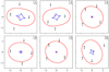 |
Fig. 1. Geometry of the six lenses in our mock sample. The outer red curves are the critical curves and the inner blue diamond-shaped curves are the caustics. Images are shown as black dots labelled by increasing time delay and the true source positions are the red dots near the centres. The scale is given in arcseconds. |
The only explicit free parameters for the MCMC simulation are the cosmological parameters. The image positions are fitted implicitly within the loop by analytically minimising the deviations of the image positions and the redshifts. This χ2 is then used for the likelihood of the outer MCMC loop. Tests show that this accelerated approach introduces only negligible errors. The time delays themselves can be used directly because of their extreme precision. Their uncertainty matters only in so far as the time delays are used to determine the relative redshifts.
As our measurement uncertainties, we assume 10−14 for the relative redshifts and 0.5 mas for the image positions (0.35 mas for each component). It so happens that these errors influence the resulting uncertainty to a very similar extent, so that both have to be reduced for a significant improvement.
Firstly, we investigate how well individual parameters can be determined from individual lenses, assuming that all others are known. Table 2 shows the resulting uncertainties for the Hubble constant and the matter density, assuming the other is known and a spatially flat Universe with w = −1. We find that the uncertainties vary strongly from lens to lens, which means that more realistic samples should be investigated in the future. Generally, we find that more asymmetric lenses (visible as larger caustics) are better, but the details have to be worked out.
Uncertainties (standard deviations) of H0 and ΩM determined individually (assuming the other and w known) from the six lenses.
Because a measurement of the Hubble constant alone is not equipped to solve the current parameter tension, we also simulate fits of sets of parameters to the full ensemble of lenses. Figure 2 and Table 3 show results for the Hubble constant and matter density for a flat Universe with w = −1. Figure 3 and Table 4 add w as free parameter. Some of the correlations between these parameters are significant, but none are so extreme to preclude the determination of all. This may change if we relax the condition of a spatially flat Universe.
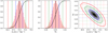 |
Fig. 2. Posterior distribution of H0 and ΩM using all lenses simultaneously. Two left panels show the marginalised distributions. Vertical dashed lines are the 1, 2, 3σ limits (68.3%, 95.4%, 99.7%, respectively, in blue, green, red) and the median (black solid). The total plot range is adapted to the 3σ range. The right panel shows the two-dimensional distribution. The marginalised limits are included as shaded horizontal and vertical lines. The contours show the 2-dimensional 1, 2, 3σ limits, respectively, in blue, green, red. The total range is the same as in the left panels. |
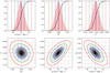 |
Fig. 3. Posterior distribution of H0, ΩM and w using all lenses simultaneously. The upper row shows marginalised distributions for individual parameters, the lower row for all combinations of two. See Fig. 2 for a detailed description. |
Uncertainties (standard deviations) of H0 and ΩM determined from all six lenses combined for a spatially flat Universe with w = −1.
Uncertainties (standard deviations) of H0, ΩM, and w determined from all six lenses combined for a spatially flat Universe.
The potential for the achievable accuracy with this approach is competitive with that achievable by combinations of other methods, particularly with regard to the matter density and the equation of state of dark energy. It remains to be seen how realistic our assumptions are.
5. Caveats
There are a number of effects that can perturb the measured time delays and (more importantly) their time-derivatives. Most relevant is the proper motion, which can be determined and implicitly corrected for quad systems as shown above. The accuracy of this correction depends on the astrometric accuracy. The radial motion is also discussed above, where we note that the motion of the Earth relative to the background metric must be taken into account.
5.1. Motion of the observer
As explained above, we have to correct the arrival times of bursts for a number of effects. Firstly, there is the diurnal motion of the observer (which is extremely well-known) and the Earth’s orbit around the Solar system barycentre. Relative to the known planets and the Sun, this motion is certainly known to better than 300 m, which would correspond to the claimed timing accuracy of one microsecond. Unfortunately we need to know the motion relative to a local inertial frame. Should there be additional large unknown masses in the Solar system, for instance, an unknown distant planet, its direct influence on the motion of the inner planets may be small, but it does introduce a relative motion between the true barycentre and the one derived from the known planets.
With timing observations of a binary pulsar, relative radial acceleration between the pulsar and us can be measured very accurately. Verbiest et al. (2008) did this for PSR J0437–4715 with an accuracy corresponding to a/c of 1.2 × 10⁻¹⁹ s−1, which is about 5% of the Hubble constant. Within the measurement accuracy, the result is consistent with the Galactocentric acceleration and kinematic effects, with a remaining uncertainty of any unmodelled contributions of 6 × 10⁻¹⁹ s−1. This constraint was improved by Deller et al. (2008) with a new measurement of the parallax, with a limit of 1.6 × 10⁻¹⁹ s−1 at the 2-σ level. The acceleration measurement itself was also improved by Reardon et al. (2016) by an order of magnitude and is now at an uncertainty of 1.2 × 10⁻²⁰ s−1. It is still consistent with the Galactic and kinematic contributions.
For our acceleration relative to an inertial frame, we have to consider the total Galactocentric acceleration of the observer. This amounts to a/c = 8 × 10⁻¹⁹ s−1 or about one third of the Hubble constant. It is thus a very relevant effect that must be corrected for. MacMillan et al. (2019) show an overview of results from Galactic kinematics compared with VLBI measurements via the resulting apparent proper motion of extragalactic sources. These measurements include the acceleration of the Milky Way towards the average Hubble flow. Their accuracy (on the order of 6 × 10⁻²⁰ s−1) is currently sufficient to correct lensing redshift measurements for most of the effect, but further improvements are required.
With a sufficiently large sample of lensed FRBs, our local acceleration can be measured (and corrected) from the observed lensing redshifts because its effect is position dependent. This can potentially even be used to improve the Solar system ephemeris, to find unknown masses in the outer Solar system, and to study the acceleration of the Milky Way relative to the background. This approach carries the disadvantage that it can absorb potential large-scale anisotropies, which may then go unnoticed.
5.2. Evolution of lens structure
Our entire argument is based on the assumption that the mass distribution of the lens stays constant with time. According to Table 1 we are measuring relative changes of time delays on the order 2 × 10⁻¹⁰, corresponding to substantial changes over time scales of 10 Gyr, which means that even small violations of the assumption will matter. Typical rotational time scales are much smaller, but they are not relevant as long as the rotating mass distribution is symmetric. Major encounters or mergers will certainly introduce large perturbations, but we hope that such systems can be excluded based on their morphology. Walker (1996) discusses how gravitational lensing by moving stars in the Milky Way might influence pulsar timing, discussing effects that are almost always too small to be relevant.
Other changes are still of concern and have to be investigated in the future using structure formation simulations. These not only have the potential to provide the mass distribution at a given moment, but also the changes over time. Even if they do not reproduce realistic mass distributions of galaxies exactly, they will allow us to estimate typical effects on observed lensing-induced differential redshifts.
5.3. Masses near the line of sight
Our approach of combining time delays and their time derivatives (redshifts) allows us to eliminate the unknown mass distribution of the lens and break the mass-sheet degeneracy, as long as all unknown masses are at the same known redshift. Additional over- or underdensities along the line of sight will not automatically be corrected for. Because even their total static effect is usually small (e.g. Millon et al. 2020b), we expect that the remaining error in our method will not introduce large systematics, but this has to be investigated in detail.
More worrying are the potential effects on the time derivatives due to moving or evolving masses near the line of sight. Their influence has to be studied, again, likely based on simulations of the large-scale structure formation.
Masses outside of the main lens will have only a small effect. The zeroth-order (in position) redshift caused by the evolving lensing potential does not effect the relative redshifts. The first order is expected to be much lower and absorbed in the proper motion, for which it introduces only a small error. Only higher orders remain, which are sufficiently low for masses that are not too close to the line of sight. It is thus expected that most lens systems should not be problematic, but this has to be worked out quantitatively.
5.4. Astrometry of lensed images
The ability to measure and correct for the relative proper motions relies on accurate measurements of the relative positions of the lensed images, with uncertainties on sub-mas levels. For bright persistent sources, for instance, lensed AGN, this is not problematic. With VLBI at L-band near 1.4 GHz we can achieve resolutions of a few mas, even better at higher frequencies. The achievable positional uncertainty scales with the resolution divided by the S/N, such that relative positions better than 0.1 mas, at least for pointlike sources, are routinely achieved.
For FRBs, the situation is more difficult. Firstly, they are short, so that the S/N will generally be lower than for AGN sources. With careful gating (S/N-based weighted averaging), it is still realistic to achieve an S/N of 100, which would be sufficient8. Another difficulty is the very poor image fidelity due to the sparse UV coverage for individual bursts or images. Even with proper model-fitting to the observed visibilities, this causes highly non-Gaussian errors, which can only be beaten down by combining several bursts.
Finally, we can only see one image at a time, so the positions cannot be measured directly relative to each other, but have to be relative to a nearby calibrator source using phase-referencing. This always leaves residual errors due to the atmosphere and ionosphere. In principle, these can be reduced by observing a number of reference sources around the target, but if they are not within the same primary beam of the telescopes, we have to alternate scans of target and references, which means we may miss individual bursts. Alternatively, we can point at the target and detect bursts in realtime to move to calibrators directly after a burst. This, however, is not a standard VLBI observing mode.
For the first repeating FRB, Marcote et al. (2017) achieved an accuracy of 2–4 mas per axis by combining four bursts. The second VLBI localisation of another FRB by Marcote et al. (2020) had a similar accuracy even for individual bursts. There is certainly room for significant improvement, but the astrometry will nevertheless be challenging.
In addition to VLBI, we can also use the timing of the lensed burst images year-round to measure or improve the astrometry, which is similar to the technique for determining positions from pulsar timing. If we have a frequently repeating FRB with good coverage along the Earth’s orbit around the Sun, the effects of the orbit can be disentangled from the long-term differential redshifts. The orbit itself is then a lever arm of 1 AU. With a timing accuracy of one microsecond9, this corresponds to a positional accuracy of about 0.4 mas per measurement, unaffected by the atmosphere or ionosphere. The timing measurement requires much less effort than a full global VLBI experiment, so that it can be repeated for very many, maybe thousands of bursts, with the corresponding increase in precision.
5.5. Microlensing
We have to distinguish between two types of microlensing. The first is due to individual masses along the line of sight, as analysed by Chang & Refsdal (1979). Even if a large fraction of dark matter exists in the form of compact masses, the chance of lensing is small for any given line of sight and our proposed method will generally not be affected. This type of microlensing in FRBs has already been proposed to study the abundance of compact objects by Muñoz et al. (2016), who argue that masses in the range 10–100 M⊙ can be detected or constrained using incoherent methods. Using spectral features in the emission caused by (coherent) interference between the lensed images, Eichler (2017) describe how the range probed can be extended to much lower masses. The typical order of magnitude of the time delay between lensed images of a point-mass, assuming a modest amplification ratio, is given by the light-crossing time of the Schwarzschild radius, which is 10 μs for one Solar mass and scales proportionally to the mass.
What is potentially more problematic for our application is microlensing caused by the dense ensemble of masses in the lensing galaxy. Because the density must be high for macrolensing to occur, macro-images will always be affected by some degree of microlensing. Microlensing by the star field can produce a high number of subimages but, overall, only a few of them contribute significantly to the total flux (Saha & Williams 2011). The probability distribution of this number also depends on the type of image (minimum, maximum, or saddle-point of the arrival-time function). For known (non-FRB) lens systems, the micro-images cannot be resolved, not even with VLBI observations of radio lenses. The only observed signature is the total amplification, and its variation seen in light curves. Astrometric effects are slowly getting in reach now for the GAIA satellite.
Time delays in this type of microlensing have not been investigated thus far. Our preliminary simulations indicate that typical time delays between the brighter micro-images are on the same order of magnitude as the corresponding single-lens time delays, or larger by a factor of only a few. For a Solar mass, thus we have to expect delays in the range of a few times 10 μs. This is well above the assumed accuracy of one microsecond (Table 1) and thus potentially detrimental for our proposed cosmological application of (macro-) time delays. Luckily the situation is not hopeless. What is relevant for our purposes is not so much the accuracy of the absolute time delays, but the accuracy of their rate of change. For a rough estimate of the typical time scale, we can divide the Einstein radius of typical masses (a few times 1011 km, angular scale a few μarcsec) by the typical transverse velocity, which results in many decades. Because we were assuming to measure changes over approximately three years, the effect is reduced by at least an order of magnitude, which brings it into an acceptable range.
We can measure the wave field, which enables us to distinguish the microlensed images via their time delays. Generally, we expect there to only be a few relevant subimages, so that we can monitor their relative separations over the years and use this data to estimate the possible error on the derived macro time delays. The micro time delays can be measured with nanosecond precision, which provides invaluable and entirely new information about the mass distribution and motion of compact objects in the lensing galaxies. In contrast to optical microlensing studies, in which most constraints are degenerate with the source size, we can directly measure micro time delays (which are a measure for the masses) and their changes over time (which are a measure of their kinematics). Both the potential for dark-matter studies and the possible problematic influence on the cosmological application have to be studied in detail in the future.
5.6. Interstellar scattering
The interstellar plasma has a refractive index for radio waves that is proportional to the electron density and to λ2. Density fluctuations cause deflections that are similar in nature to microlensing and can produce a high number of subimages that interfere with each, which we observe as interstellar scintillation. The effect is independent for the lensed macro-images, so that it spreads out the correlation between the measured wave fields and reduces the accuracy of a macro-delay determination. Sophisticated methods have been developed to study the effect in scintillating pulsars, but these rely on a good time coverage in order to model the scattering field. For FRBs we do not have this luxury, but have to try and reduce the effect as much as possible by observing at high frequencies. Scattering sizes roughly scale with λ2.2, corresponding time delays with λ4.4.
The range of scattering delays depends critically on the line of sight. For scattering within the Milky Way, low Galactic latitudes generally show much stronger effects. Using the NE2001 model for the distribution of free electrons in the Milky Way (Cordes & Lazio 2002), we find that for 1.4 GHz the scattering delay is always below 1 μs for Galactic latitudes above ±20°, and mostly even above ±10°, so that the redshift accuracy will stay within our assumed limits for most of the sky. In known FRBs, it has been determined that the intergalactic medium generally adds much less scattering than the Milky Way. Scattering in the host is extremely variable. By finding FRBs at low frequencies, for instance with CHIME, those with low scattering in the host are automatically selected.
An additional important factor in lensed FRBs may be the scattering in the lensing galaxy itself, or in the intergalactic or intracluster medium around it. If the lens scatters as strongly as the disk of the Milky Way, the range of scattering delays would indeed make a delay measurement with the required accuracy impossible. To our advantage, the most efficient gravitational lenses are massive elliptical galaxies. As result of their old population of stars and the corresponding absence of H II regions and supernova remnants, their already thin interstellar medium is also calm without strong fluctuations in the plasma density. They are thus expected to have levels of scattering that are orders of magnitude lower, if diffractive scattering can happen at all. Admittedly, the physical processes involved in scattering are not even fully understood in the Milky Way and the extrapolation to elliptical galaxies might turn out to be too optimistic.
Because of the strong frequency dependence, we can always reduce the effect by going to higher frequencies. This will generally be necessary if we want to study the delays of micro-images in detail. If, in the worst case, the scattering is too strong to measure time delays with accuracies of a microsecond, we will notice immediately because no sharp peak will be found in the coherent correlation. The accuracy can be estimated from the width of the peak and there is no danger that an unexpected large error would go unnoticed.
5.7. Ionospheric and atmospheric delays
These effects are relevant for VLBI-astrometry of the lensed images, but can be neglected for the redshifts derived from measured time delay changes. The troposphere has an effect of less than 10 nanoseconds at zenith and most of that is predictable. The effect of the ionosphere is frequency-dependent and very variable. The column density of electrons is almost always below 100 TECU (one TECU corresponds to 1016 m−2), which at 1 GHz causes delays of about 130 nanoseconds. The delay scaling is inversely proportional to the observing frequency squared and it may generally, thus, be neglected.
5.8. Finding lensed FRBs
The main caveat is that no gravitationally lensed FRB repeaters are known thus far. The ASKAP and CHIME telescopes are already finding FRBs at a high rate, which, with a lensing fraction of about one in 1000, would mean about one lensed FRB per year. However, because they cover only a small fraction of the sky at a given moment, they will almost always miss the lensed copies of bursts. Researchers might try to identify lensed candidates by their expected microlensing signature and then try to find repeats and lensed copies with targeted observations, but this approach would hardly find enough suitable systems.
What is needed for the search of gravitationally lensed FRBs is a telescope that continuously monitors a significant fraction of the sky without interruption, so that no bursts or lensed images would be missed. A good option is to concentrate on the circumpolar region, for example north of the declination 50°, which always has an elevation greater than 10° at latitudes above 50°. This patch corresponds to more than one tenths of the entire sky, or about 20 times the field of view of CHIME. At the same level of sensitivity as CHIME, we expect to find 40 FRBs per day (Fonseca et al. 2020) or a substantial number of lensed ones per year.
The most efficient instrument for such a wide-field monitoring is a regular array of antennas or small dishes with a beamformer based on a two-dimensional Fast Fourier Transform as proposed by Otobe et al. (1994) and Tegmark & Zaldarriaga (2009). A one-dimensional version of this approach is already being used by CHIME-FRB (Ng et al. 2017; Masui et al. 2019), and an application for the two-dimensional case is straight forward. Appropriate antenna arrays were developed as design studies for the Square Kilometre Array (SKA). The EMBRACE test array (Torchinsky et al. 2015, 2016) is an 8 × 8 m array consisting of 4600 dual-polarisation (only one fully equipped) elements for the frequency range between 900–1500 MHz. The original analogue beamformer cannot directly be used for the FFT-based beamformer design, but we are considering options to combine the existing array or a variant of it with a CHIME-like beamformer as a first step in the direction of a sensitive wide-field FRB search instrument.
6. The gravitational lens as interferometer
The notion of mutual coherence between gravitationally lensed images has already been discussed by Schneider & Schmid-Burgk (1985) and others. Within the framework of our discussion, we can think of the gravitational lens as a huge intergalactic interferometer, the arms of which are given by individual lensed images. We assume that these have an apparent separation of θ, which corresponds to a baseline in the lens plane of L = Dd θ. The angular resolution at a wavelength of λd (measured in the lens plane) is then λd/L. The corresponding linear resolution in the source plane we call Δx, which would be seen by the observer as the angular resolution Δθ, with
 (42)
(42)
 (43)
(43)
Here, we assumed that the “arms of the interferometer” are fixed. In reality, however, the images will slightly shift with position in the source plane, which adds geometric and potential components to the phase difference between parts of the source. Fortunately, these effects are cancelled out because of Fermat’s principle, as discussed in Sect. 3.5. A gravitational lens really is equivalent to a fixed Young’s double slit.
Using our order-of-magnitude estimates from Table 1, neglecting the lens redshift and the differences between distance parameters, and using a wavelength of λ0 = 20 cm, we get a linear resolution of 40 km and an angular resolution of 3 × 10⁻¹⁶ arcsec, or about 0.3 femto-arcsec. With the actual values from our lens sample, we find (for a 2 arcsec image separation) linear and angular resolutions of 4–11 km and 15–53 atto-arcsec, respectively.
The images are mutually coherent only as long as this lens-interferometer does not resolve all their structures, in other words, for only as long as the sources have structures on scales below about ten kilometres. We emphasise that most of this paper relies on this assumption because otherwise we could not achieve the required precision in the measured redshifts. Cho et al. (2020) find narrow structures in FRB 181112 with rise time of down to 15 μs, or 10 μs when correcting for redshift. This corresponds to a maximum source size of 3 km, which is small enough to maintain coherence.
As long as there is at least some level of mutual coherence, we can now use the lens as interferometer with (for a quad) six independent baselines. At the very least, we can compare amplitudes of correlations (“visibilities”) between baselines and in this way measure the sizes of source components. It remains to be discussed how well the effects of microlensing and interstellar scattering can be corrected for in the analysis. These will be different for the different macro-images, so that they can be treated as responses of the virtual interferometer stations corresponding to the images. The resolution corresponding to the subimages caused by these effects is much poorer, so that they will not introduce differential effects across the FRB source. In other words, we should be able to measure phase differences between the visibilities of subcomponents of the source, or even between subsequent bursts. Depending on the achievable S/N we may be able to measure relative positions with accuracies of a kilometre or even better. The extreme precision of such a measurement at cosmological distances cannot be admired enough.
We cannot expect to measure consistent phases between bursts that are separated more than the interstellar scintillation timescale. With the assumed reduced precision of a microsecond, we can measure positional offsets between bursts with an accuracy on the order of 50 femto-arcsec or typically 104 km, which is still impressive for sources at Gpc distance. Uniform motion will be absorbed in the relative proper motion, but any deviation from that, for example, due to orbital motion, will be easily measurable with exquisite precision. Dai & Lu (2017) discuss this and other aspects of motion of the source, lens, and observer in the context of lensed FRBs; however, these authors only consider incoherent measurements with millisecond accuracy.
7. Discussion
With gravitationally lensed FRBs, time delays can potentially be measured very accurately, not only to milliseconds, as expected from their short nature, but even to microseconds or even nanoseconds because we can measure the wave fields of the images and correlate them coherently. For repeating FRBs, this presents the opportunity to measure how time delays change over timescales of months and years. These changes are described as differential redshifts between the images. Here, we derive how the differential redshifts are related to parameters of the lens and the cosmological model. We find that in quadruply imaged systems we have sufficient information to be able to combine the time delays themselves with their time-derivatives (or the redshifts) to eliminate uncertainties from the a priori unknown mass distribution of the lens entirely.
In classical gravitational lensing, where mass models are fitted to the observable image configuration (and perhaps other parameters such as the velocity dispersion of the lens), fundamental parameter degeneracies remain that cannot be removed without further assumptions. Because the true mass distributions are unknown, it is difficult to estimate the biases introduced by the assumptions. The mass-model uncertainties are generally seen as the most serious source of systematic errors in lensing.
Removing this main uncertainty with lensed FRBs does not come at no cost: the differential redshifts are extremely small and a number of additional effects have to be taken into account in the analysis. Most important is the relative transverse motion of the source, lens, and observer. This contribution from proper motion is about three orders of magnitude larger than the cosmological effect, but for quad systems it can be determined and removed, as long as the relative image positions are accurately known. Such measurements are possible with VLBI.
Kochanek et al. (1996) argue that proper motion measurements at cosmological distances would be very valuable to study our motion relative to a rest frame defined by external galaxies independent of the CMB dipole or to study local kinematics. They estimate that with VLBI, normal peculiar velocities of galaxies are “too small for direct detection given current life expectancies”. VLBI precision has improved since then and life expectancies have generally increased, but the statement is still true. The proper motion from Table 1 corresponds to less than one μarcsec over a decade, which is beyond detectability with VLBI. Kochanek et al. (1996) propose to measure quad lenses with VLBI to utilise the lensing magnification to boost the motion and to provide nearby reference sources but even then, obtaining a measurement is challenging. The relative redshift induced by proper motion, on the other hand, enables very accurate measurements and any conclusions will only be limited by the sample variance. Large-scale systematic motion, such as cosmic rotation on sub-horizon scales, can then be studied with high accuracy, as well as other unexpected effects.
This is not the first time that time-derivatives of time delays have been discussed in the literature. Zitrin & Eichler (2018) investigate a number of aspects of observing cosmic expansion and other secular changes (including transverse motion) in realtime. They calculate rates of change of time delays for special mass models, but they do not combine time delays and their derivatives to determine cosmological parameters, nor do they describe how quad systems can be used to separate transverse motion and cosmology. Piattella & Giani (2017) calculate expected drifts of redshifts, image positions, and time delay for point-mass lenses, but do not discuss which quantities can be measured with lensed FRBs.
At this moment it is not possible to estimate achievable accuracies for cosmological parameters reliably because many important parameters are unknown. Typical source redshifts are the most important in this regard, but we also find that subtle details of the mass distribution of lensing galaxies can lead to very different accuracies of our proposed method. As a first attempt we used a simulated sample of lenses (not claimed to be representative) as basis for an assessment of the achievable results. With six lenses we find that accuracies of a few percent may be realistic for the Hubble constant, the matter density, and the equation-of-state parameter, w, of the dark energy. We repeat that these estimates are based on strong assumptions for the lenses and, currently, for the assumed spatial flatness of the Universe.
Given that the classical approach of lensing time delays is producing competitive results despite the known limitations, it should also be applied to lensed FRBs. Li et al. (2018) and Liu et al. (2019) argue that lensed FRBs provide better constraints on the lens mass distribution than lensed AGN because of the absence of a bright dominant component in the host. Combining both methods is probably the best option. At the very least, we can use classical modelling for lensed FRBs and use the differential redshifts as additional constraints. Even if this does not improve the cosmological result, using the time delays themselves in addition to the redshifts provides one additional constraint on the mass distribution – it is only one because we add three equations for the relative time delays but we also need to add the source position as free parameter.
Further investigations of a number of aspects are needed, most importantly: the effects of evolution of the mass distribution in the main lens and along the line of sight. These can be estimated based on structure formation simulations. Besides the unknown redshift distribution, we may use lens models of existing well-studied non-FRB lenses and determine how well those lenses would be suited for cosmology based on the assumption that their sources could be FRBs.
Microlensing is another important effect. According to our estimates, it does not invalidate our approach but, rather, it provides entirely new information on the masses in the lenses and may in this way shed some light on the dark matter problem. Time delays between micro-images cannot be measured with other sources and their properties still have to be investigated theoretically.
The physical nature of FRB sources is currently not understood at all, but we know that they must either be small or at least have subcomponents of at most a few kilometres in size. This means there is no chance to resolve their structures with any astronomical instrument, not even with space VLBI. Gravitational lenses can be used as a natural telescopes, not just in the classical mode of magnifying the sources, but by providing interferometric baselines on the scale of a galaxy. The electromagnetic fields of lensed images can be correlated with each other and interferometric visibilities can be produced, which would resolve structures of a few kilometres at cosmological distances. This approach cannot be used for standard AGN sources because they would be fully resolved out. Having small structures is not only necessary for measuring highly precise coherent delays, but the correlations will resolve structures and help studying the sources in turn.
Besides additional work on the theoretical understanding, it is now of the highest importance that instruments are built that are equipped with the capacity to find gravitationally lensed repeating FRBs in sufficient numbers. New arrays such as ASKAP and CHIME completely changed the game regarding the number of FRBs, but they are not optimised for the discovery of lensed ones because they generally end up missing most of the lensed images. Continuous coverage of a large field on the sky appears to be the best way of finding lensed FRBs. The required technology exists, along with even some of the hardware, and FFT telescopes can be built as efficient lensed-FRB machines. The potential for cosmology and other aspects of astrophysics is certainly within reach and worth the effort.
When using this absolute phase delay, a frequency-independent phase shift depending on the type of image has to be taken into account. In principle, this could even be used to determine the types of images.
We use a slightly sloppy notation in which the functions R(t), R(η) and R(z) are written with the same letter.
With +const, we denote an additive term that does not depend on θ and therefore cancels in time delays between images. This constant can be different in different equations.
Of course, physical effects should only depend on relative motion. A situation with a moving source can be Lorentz-transformed to that of a moving observer. The relativistic length contraction does not matter here because it is of second order. More important is the effect of redefined simultaneity. In one situation, we define the distance at the moment of emission and in the other at the moment of observation. The relative motion between these two moments accounts for the difference in the two descriptions.
This is not a physical effect in the sense of a deceleration but because the object moves into a region with a slightly different Hubble flow, the relative speed is reduced.
We emphasise that the knowledge of this restriction is not used when deriving cosmological parameters from the simulated data. This is different from fitting isothermal models.
AstroPy (Astropy Collaboration 2013, 2018) was used for the cosmological calculations and results were checked against our own integration code that is more general and can also compute Dyer-Roeder distances for inhomogeneous models.
Marcote et al. (2020) find bursts with SNR of about 50 for the 100-m Effelsberg telescope, even without optimal gating of the small-scale structure.
We repeat that this accuracy is not available for lags between bursts, but only for lensing delays between images. If the time delays are a good fraction of a year, we still have very accurate measurements between different Earth positions, which is sufficient for a good localisation.
Acknowledgments
L.G.S. is a Lise Meitner independent research group leader and acknowledges funding from the Max Planck Society. Ue-Li Pen receives support from Ontario Research Fundresearch Excellence Program (ORF-RE), Canadian Foundation for Innovation (CFI), Simons Foundation, and Alexander von Humboldt Foundation. He acknowledges the support of the Natural Sciences and Engineering Research Council of Canada (NSERC, funding reference number RGPIN-2019-067, CRD 523638-201). He also receives substantial support from the Max-Planck-Institut für Radioastronomie.
References
- Astropy Collaboration (Robitaille, T. P., et al.) 2013, A&A, 558, A33 [NASA ADS] [CrossRef] [EDP Sciences] [Google Scholar]
- Astropy Collaboration (Price-Whelan, A. M., et al.) 2018, AJ, 156, 123 [Google Scholar]
- Bannister, K. W., Deller, A. T., Phillips, C., et al. 2019, Science, 365, 565 [NASA ADS] [CrossRef] [Google Scholar]
- Biggs, A. D., & Browne, I. W. A. 2018, MNRAS, 476, 5393 [CrossRef] [Google Scholar]
- Birkinshaw, M., & Gull, S. F. 1983, Nature, 302, 315 [NASA ADS] [CrossRef] [Google Scholar]
- Browne, I. W. A., Wilkinson, P. N., Jackson, N. J. F., et al. 2003, MNRAS, 341, 13 [NASA ADS] [CrossRef] [Google Scholar]
- Buchner, J. 2016, PyMultiNest: Python interface for MultiNest, Astrophysics Source Code Library [record ascl:1606.005] [Google Scholar]
- Buchner, J., Georgakakis, A., Nandra, K., et al. 2014, A&A, 564, A125 [NASA ADS] [CrossRef] [EDP Sciences] [Google Scholar]
- Chang, K., & Refsdal, S. 1979, Nature, 282, 561 [Google Scholar]
- Chatterjee, S., Law, C. J., Wharton, R. S., et al. 2017, Nature, 541, 58 [NASA ADS] [CrossRef] [Google Scholar]
- Cheung, C. C., Larsson, S., Scargle, J. D., et al. 2014, ApJ, 782, L14 [NASA ADS] [CrossRef] [Google Scholar]
- CHIME/FRB Collaboration (Amiri, M., et al.) 2018, ApJ, 863, 48 [NASA ADS] [CrossRef] [Google Scholar]
- CHIME/FRB Collaboration (Amiri, M., et al.) 2019, 566, 235 [Google Scholar]
- Cho, H., Macquart, J.-P., Shannon, R. M., et al. 2020, ApJ, 891, L38 [CrossRef] [Google Scholar]
- Cooke, J. H., & Kantowski, R. 1975, ApJ, 195, L11 [CrossRef] [Google Scholar]
- Cordes, J. M., & Lazio, T. J. W. 2002, ArXiv e-prints [arXiv:astro-ph/0207156] [Google Scholar]
- Dai, L., & Lu, W. 2017, ApJ, 847, 19 [NASA ADS] [CrossRef] [Google Scholar]
- Deller, A. T., Verbiest, J. P. W., Tingay, S. J., & Bailes, M. 2008, ApJ, 685, L67 [NASA ADS] [CrossRef] [Google Scholar]
- Dyer, C. C., & Roeder, R. C. 1972, ApJ, 174, L115 [NASA ADS] [CrossRef] [Google Scholar]
- Dyer, C. C., & Roeder, R. C. 1973, ApJ, 180, L31 [CrossRef] [Google Scholar]
- Eichler, D. 2017, ApJ, 850, 159 [NASA ADS] [CrossRef] [Google Scholar]
- Erkal, D., Belokurov, V., Laporte, C. F. P., et al. 2019, MNRAS, 487, 2685 [NASA ADS] [CrossRef] [Google Scholar]
- Falco, E. E., Gorenstein, M. V., & Shapiro, I. I. 1985, ApJ, 289, L1 [Google Scholar]
- Feroz, F., Hobson, M. P., & Bridges, M. 2009, MNRAS, 398, 1601 [NASA ADS] [CrossRef] [Google Scholar]
- Fonseca, E., Andersen, B. C., Bhardwaj, M., et al. 2020, ApJ, 891, L6 [NASA ADS] [CrossRef] [Google Scholar]
- Gorenstein, M. V., Falco, E. E., & Shapiro, I. I. 1988, ApJ, 327, 693 [NASA ADS] [CrossRef] [Google Scholar]
- Kantowski, R. 1969, ApJ, 155, 89 [NASA ADS] [CrossRef] [Google Scholar]
- Kochanek, C. S. 2020, MNRAS, 493, 1725 [CrossRef] [Google Scholar]
- Kochanek, C. S., Kolatt, T. S., & Bartelmann, M. 1996, ApJ, 473, 610 [NASA ADS] [CrossRef] [Google Scholar]
- Kopeikin, S. M., & Schäfer, G. 1999, Phys. Rev. D, 60, 124002 [NASA ADS] [CrossRef] [MathSciNet] [Google Scholar]
- Li, Z.-X., Gao, H., Ding, X.-H., Wang, G.-J., & Zhang, B. 2018, Nat. Commun., 9, 3833 [NASA ADS] [CrossRef] [Google Scholar]
- Liu, B., Li, Z., Gao, H., & Zhu, Z.-H. 2019, Phys. Rev. D, 99, 123517 [CrossRef] [Google Scholar]
- Lorimer, D. R., Bailes, M., McLaughlin, M. A., Narkevic, D. J., & Crawford, F. 2007, Science, 318, 777 [NASA ADS] [CrossRef] [PubMed] [Google Scholar]
- MacMillan, D. S., Fey, A., Gipson, J. M., et al. 2019, A&A, 630, A93 [NASA ADS] [CrossRef] [EDP Sciences] [Google Scholar]
- Marcote, B., Paragi, Z., Hessels, J. W. T., et al. 2017, ApJ, 834, L8 [NASA ADS] [CrossRef] [Google Scholar]
- Marcote, B., Nimmo, K., Hessels, J. W. T., et al. 2020, Nature, 577, 190 [NASA ADS] [CrossRef] [Google Scholar]
- Marlow, D. R., Rusin, D., Jackson, N., et al. 2000, AJ, 119, 2629 [NASA ADS] [CrossRef] [Google Scholar]
- Masui, K. W., Shaw, J. R., Ng, C., et al. 2019, ApJ, 879, 16 [CrossRef] [Google Scholar]
- Millon, M., Galan, A., Courbin, F., et al. 2020a, A&A, 639, A101 [CrossRef] [EDP Sciences] [Google Scholar]
- Millon, M., Courbin, F., Bonvin, V., et al. 2020b, A&A, 640, A105 [CrossRef] [EDP Sciences] [Google Scholar]
- Molnar, S. M., & Birkinshaw, M. 2003, ApJ, 586, 731 [NASA ADS] [CrossRef] [Google Scholar]
- Muñoz, J. B., Kovetz, E. D., Dai, L., & Kamionkowski, M. 2016, Phys. Rev. Lett., 117, 091301 [NASA ADS] [CrossRef] [Google Scholar]
- Ng, C., Vanderlinde, K., Paradise, A., et al. 2017, in 32nd URSI GASS. [arXiv:1702.04728] [Google Scholar]
- Otobe, E., Nakajima, J., Nishibori, K., et al. 1994, PASJ, 46, 503 [Google Scholar]
- Piattella, O. F., & Giani, L. 2017, Phys. Rev. D, 95, 101301 [CrossRef] [Google Scholar]
- Planck Collaboration VI. 2020, A&A, 641, A6 [NASA ADS] [CrossRef] [EDP Sciences] [Google Scholar]
- Pyne, T., & Birkinshaw, M. 1993, ApJ, 415, 459 [CrossRef] [Google Scholar]
- Reardon, D. J., Hobbs, G., Coles, W., et al. 2016, MNRAS, 455, 1751 [NASA ADS] [CrossRef] [Google Scholar]
- Refsdal, S. 1964a, MNRAS, 128, 295 [NASA ADS] [CrossRef] [MathSciNet] [Google Scholar]
- Refsdal, S. 1964b, MNRAS, 128, 307 [NASA ADS] [CrossRef] [Google Scholar]
- Refsdal, S. 1966, MNRAS, 132, 101 [CrossRef] [Google Scholar]
- Saha, P., & Williams, L. L. R. 2011, MNRAS, 411, 1671 [NASA ADS] [CrossRef] [Google Scholar]
- Schneider, P., & Schmid-Burgk, J. 1985, A&A, 148, 369 [Google Scholar]
- Schneider, P., & Sluse, D. 2014, A&A, 564, A103 [NASA ADS] [CrossRef] [EDP Sciences] [Google Scholar]
- Spitler, L. G., Scholz, P., Hessels, J. W. T., et al. 2016, Nature, 531, 202 [NASA ADS] [CrossRef] [Google Scholar]
- Tegmark, M., & Zaldarriaga, M. 2009, Phys. Rev. D, 79, 083530 [NASA ADS] [CrossRef] [Google Scholar]
- Tendulkar, S. P., Bassa, C. G., Cordes, J. M., et al. 2017, ApJ, 834, L7 [NASA ADS] [CrossRef] [Google Scholar]
- Torchinsky, S. A., Olofsson, A. O. H., Censier, B., et al. 2015, J. Instrum., 10, C07002 [CrossRef] [Google Scholar]
- Torchinsky, S. A., Olofsson, A. O. H., Censier, B., et al. 2016, A&A, 589, A77 [CrossRef] [EDP Sciences] [Google Scholar]
- Verbiest, J. P. W., Bailes, M., van Straten, W., et al. 2008, ApJ, 679, 675 [NASA ADS] [CrossRef] [Google Scholar]
- Walker, M. A. 1996, PASA, 13, 236 [CrossRef] [Google Scholar]
- Walsh, D., Carswell, R. F., & Weymann, R. J. 1979, Nature, 279, 381 [NASA ADS] [CrossRef] [PubMed] [Google Scholar]
- Wong, K. C., Suyu, S. H., Chen, G. C. F., et al. 2019, MNRAS, 498, 1420 [CrossRef] [Google Scholar]
- Wucknitz, O. 2002, MNRAS, 332, 951 [NASA ADS] [CrossRef] [Google Scholar]
- Wucknitz, O., & Sperhake, U. 2004, Phys. Rev. D, 69, 063001 [NASA ADS] [CrossRef] [Google Scholar]
- Zitrin, A., & Eichler, D. 2018, ApJ, 866, 101 [NASA ADS] [CrossRef] [Google Scholar]
Appendix A: Details of the mock lens sample
Lens model parameters: external shear, ellipticity of the potential, source position, scaling factor for time delays and the two coefficients for the redshifts.
Parameters of all the lensed images: position, potential, time delay, and redshift due to Hubble expansion.
All Tables
Uncertainties (standard deviations) of H0 and ΩM determined individually (assuming the other and w known) from the six lenses.
Uncertainties (standard deviations) of H0 and ΩM determined from all six lenses combined for a spatially flat Universe with w = −1.
Uncertainties (standard deviations) of H0, ΩM, and w determined from all six lenses combined for a spatially flat Universe.
Lens model parameters: external shear, ellipticity of the potential, source position, scaling factor for time delays and the two coefficients for the redshifts.
Parameters of all the lensed images: position, potential, time delay, and redshift due to Hubble expansion.
All Figures
|
Fig. 1. Geometry of the six lenses in our mock sample. The outer red curves are the critical curves and the inner blue diamond-shaped curves are the caustics. Images are shown as black dots labelled by increasing time delay and the true source positions are the red dots near the centres. The scale is given in arcseconds. |
| In the text | |
|
Fig. 2. Posterior distribution of H0 and ΩM using all lenses simultaneously. Two left panels show the marginalised distributions. Vertical dashed lines are the 1, 2, 3σ limits (68.3%, 95.4%, 99.7%, respectively, in blue, green, red) and the median (black solid). The total plot range is adapted to the 3σ range. The right panel shows the two-dimensional distribution. The marginalised limits are included as shaded horizontal and vertical lines. The contours show the 2-dimensional 1, 2, 3σ limits, respectively, in blue, green, red. The total range is the same as in the left panels. |
| In the text | |
|
Fig. 3. Posterior distribution of H0, ΩM and w using all lenses simultaneously. The upper row shows marginalised distributions for individual parameters, the lower row for all combinations of two. See Fig. 2 for a detailed description. |
| In the text | |
Current usage metrics show cumulative count of Article Views (full-text article views including HTML views, PDF and ePub downloads, according to the available data) and Abstracts Views on Vision4Press platform.
Data correspond to usage on the plateform after 2015. The current usage metrics is available 48-96 hours after online publication and is updated daily on week days.
Initial download of the metrics may take a while.