| Issue |
A&A
Volume 698, May 2025
|
|
|---|---|---|
| Article Number | A161 | |
| Number of page(s) | 7 | |
| Section | Cosmology (including clusters of galaxies) | |
| DOI | https://doi.org/10.1051/0004-6361/202450857 | |
| Published online | 11 June 2025 | |
The strong lensing model of MACS J0035.4−2015
1
Max-Planck-Institut für Astrophysik, Karl-Schwarzschild-Str. 1, 85748 Garching, Germany
2
Technical University of Munich, TUM School of Natural Sciences, Physics Department, James-Franck Str. 1, 85748 Garching, Germany
3
Institute of Astronomy and Astrophysics, Academia Sinica, 11F of ASMAB, No. 1, Section 4, Roosevelt Road, Taipei 10617, Taiwan
⋆ Corresponding author: chitsanupongsomma@googlemail.com
Received:
24
May
2024
Accepted:
18
February
2025
We used strong gravitational lensing to study the mass distribution of the galaxy cluster MACS J0035.4−2015, by modeling its total mass distribution. The combination of high-resolution imaging from the Hubble Space Telescope with ground-based spectroscopy from the Multi Unit Spectroscopic Explorer mounted at the Very Large Telescope allowed us to model the observed multiple image positions with ≈0.″3 precision. We find that MACS J0035.4−2015 can be best described by a combination of an elliptical dark matter halo modeled as an isothermal mass profile, with the brightest cluster galaxy and cluster members each modeled with a spherical truncated isothermal parameterization. With these assumptions, the total mass is estimated to be ≈ 6 × 10¹³ M⊙ within 100 kpc. The data and mass model presented here form the basis for future cosmological and astrophysical studies of this cluster.
Key words: gravitational lensing: strong / galaxies: clusters: individual: MACS J0035.4−2015 / cosmological parameters / cosmology: observations / dark matter / dark energy
© The Authors 2025
 Open Access article, published by EDP Sciences, under the terms of the Creative Commons Attribution License (https://creativecommons.org/licenses/by/4.0), which permits unrestricted use, distribution, and reproduction in any medium, provided the original work is properly cited.
This article is published in open access under the Subscribe to Open model.
Open Access funding provided by Max Planck Society.
1. Introduction
Gravitational lensing is a powerful tool in modern cosmology that allows us not only to measure the total projected mass distribution of galaxies and galaxy clusters, but also to detect very high-redshift sources due to its magnification properties, and to investigate the global structure and the background content of the Universe. According to different cosmological observations, for example observations of the cosmic microwave background (Planck Collaboration VI 2020; Smoot et al. 1992; Hinshaw et al. 2013), baryon acoustic oscillations (e.g., Verde et al. 2002; Eisenstein et al. 2005; Sevilla-Noarbe et al. 2021; Adame et al. 2025, and Type Ia supernovae Riess et al. (1998), Perlmutter et al. (1999), Astier et al. (2006), Suzuki et al. (2012), Scolnic et al. (2022), Rubin et al. (2025), Abbott (2024), the energy density makeup of the Universe today is essentially 5% baryonic visible matter, about 25% cold dark matter (both of which are included in the total matter density parameter, Ωm), and about 70% a form of dark energy, ΩΛ. The dark energy component is needed for the current acceleration of the expansion of the Universe, and its nature is still poorly understood.
Both gravitational strong lensing and weak lensing are very effective ways to measure the mass distribution of baryonic matter and dark matter in galaxy clusters (e.g., Tyson et al. 1990; Clowe et al. 2006; Kneib & Natarajan 2011; Natarajan et al. 2024). The strong lensing technique is based on the observed positions and time delays (when available) of multiple images of lensed background galaxies, which depend on the angular diameter distances to the lens galaxies (DL), to the background source galaxies (DS), and between the lens and source galaxies (DLS). Since distance measures in cosmology depend on the evolution of the Universe and hence on cosmological models, one can use strong lensing to constrain cosmological parameters and thus determine their relative contributions to the total energy density of the Universe.
To obtain robust estimates of the cosmological parameters, different cosmological probes are often combined as each of them has distinct parameter degeneracies and possible biases (Planck Collaboration VI 2020). Gravitational lensing is a promising technique that yields orthogonal constraints relative to some observations (Jullo et al. 2010; Caminha et al. 2016). A static strong lensing system with positions of multiple images only allows measurements of the ratio of the angular diameter distances and hence is independent of the Hubble constant, H0. Systems with time delays between multiple images, such as supernovae and quasars, can be used to place new constraints on the values of H0 and of the cosmological parameters describing the global geometry of the Universe (see, e.g., Grillo et al. 2020; Kelly et al. 2023; Pascale et al. 2025; Grillo et al. 2024; Vega-Ferrero et al. 2018).
However, to perform cosmography with strong lensing, a precise description of the mass distribution of the cluster lens is needed, which requires large numbers of constraints. Different photometric surveys, for example the Massive Cluster Survey (MACS; Ebeling et al. 2001), the Cluster Lensing And Supernova survey with Hubble (CLASH; Postman et al. 2012), the Hubble Frontier Fields (HFF; Lotz et al. 2017), and the Reionization Lensing Cluster Survey (RELICS; Coe et al. 2019), have identified thousands of multiple images deflected and distorted by massive galaxy clusters, whose apparent positions are accurate to less than an arcsecond thanks to the high spatial resolution of the Hubble Space Telescope (HST). Nonetheless, spectroscopic information is crucial for obtaining a clean sample of strong lensing constraints, and the redshift information of multiple images makes the model sensitive to the background cosmology. Extensive spectroscopic studies on lensing clusters have been carried out, notably with ground-based 8-meter class telescopes in the optical and near-infrared wavelengths (see, e.g., Richard et al. 2021; Caminha et al. 2019; Rosati et al. 2014), to complement the imaging data. These datasets enable us to construct strong lens mass models of galaxy clusters for cosmological inferences.
We investigated the cluster MACS J0035.4−2015 (hereafter MACS J0035; RA = 00:35:26.12, Dec = −20:15:44.24). We present the multiple image selection with photometric and spectroscopic data from the MACS survey in Sect. 2. The strong lensing models, methodology, and total mass reconstruction of MACS J0035 are presented in Sect. 3. Finally, the result and the future development of this work are discussed in Sect. 4. All magnitudes are in the AB system (Oke 1974; Oke & Gunn 1983).
2. Photometric and spectroscopic data
The galaxy cluster MACS J0035 (Fig. 1) was first observed by HST under the MACS program (HST program IDs 10491 and 12884; see, e.g., Ebeling et al. 2001; Horesh et al. 2010) in optical wavelengths with the filters F606W and F814W. Later, additional optical and near-infrared observations, totaling four HST orbits were obtained under the RELICS program (ID 14096; Coe et al. 2019), including the additional filters F475W, F105W, F125W, F140W, and F160W and reaching a nominal limiting detection limit of ≈27.2 to 26.5 magnitudes from the blue to near-infrared filters. These additional filters are crucial for the identification of multiple lensed images and for the selection of galaxy cluster members (CMs). The final HST catalogs and imaging reduction are described in Coe et al. (2019) and can be retrieved through the Mikulski Archive for Space Telescope1.
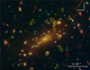 |
Fig. 1. Galaxy cluster MACS J0035 with a redshift of zL = 0.3529 at RA: 8.8588913, Dec: −20.2622861 (the coordinates mark the center of the BCG). This image includes 21 multiple images from 7 different sources, all highlighted in yellow. Diamonds indicate CMs with spectroscopic confirmation and selected from the photometry, in cyan and magenta, respectively. The BCG is marked with a blue circle. Red circles indicate multiple images with no secure spectroscopic redshift but belonging to secure families. |
Subsequently, MACS J0035 was targeted by the Multi Unit Spectroscopic Explorer (MUSE; Bacon et al. 2010) under the European Southern Observatory (ESO) program ID 0103.A-0777 (P.I. A. Edge). The observations were carried out in February and July of 2019, composed of two observational blocks each with three exposures. The total integration time is 97 minutes with a final seeing of  measured from stars in the field. We used the standard ESO recipe execution tool with the associated MUSE recipes version 2.6 (Weilbacher et al. 2016, 2020) to reduce the raw data and create the final data cube. We used the self-calibration mode of the reduction pipeline to minimize the instrumental residuals and improve the sky subtraction, especially because some of the exposures have high moon illumination of ≈50%. Moreover, we applied the Zurich Atmosphere Purge (Soto et al. 2016) to remove any persistent residuals not removed with the standard procedure.
The final data cube has ≈1′ on each side and covers the wavelength range from 4750 Å to 9350 Å. Although the seeing is not optimal, the data are good enough to measure 74 secure redshifts from 61 single extragalactic objects (where some objects are multiply lensed thus have multiple redshift measurements) and one additional star on the field of view. To measure redshifts, we extracted one-dimensional spectra of all detected sources in HST and applied a blind search in the data cube following the prescription described in Caminha et al. (2023, see their Sect. 2.2). Each redshift measurement has a quality flag (QF) to assess its robustness with the following definition: QF = 3 is a measurement using several absorptions and/or emission lines; QF = 2 is a measurement of a single spectral feature but with secure identification (such as C II lines); QF = 9 indicates the redshift was measured using one narrow, or noise emission line with insecure identification; stars have QF = 4. In this work, we considered only secure measurements (i.e., QF = 3 or 2) in order to avoid misidentifications, especially of multiple images and CMs, that could contaminate the lens model. We identified a total of 21 lensed images from 7 different background sources, as indicated on Fig. 1. Each background source has at least two secure spectroscopic confirmations. The one-dimensional MUSE spectra of multiple images is shown in Fig. 2 and the list containing the coordinates and redshift values is presented in Table 1. In Table 2 we present the first few rows of the redshift catalog and the full version is available in the electronic version of the manuscript, or upon request to the authors.
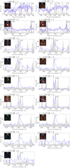 |
Fig. 2. Spectra of multiply lensed sources. Blue lines indicate the spectroscopic data and gray regions of variance. Vertical lines show the main spectral features present in each wavelength range. In cases where the continuum is clearly detected, the red line corresponds to the template used to estimate the exact redshift. The small HST cutouts in the top-left region of each panel are 2 arcsec per side. |
Catalog of the multiple images used as model constraints.
MUSE redshift catalog (extract).
3. Strong lensing model
This section focuses on the methodology to model the total mass distribution of the galaxy cluster MACS J0035 by assuming a fixed cosmological model with parameters given by H0 = 6.93 km/s/Mpc, Ωm = 0.287 and Ωm + ΩΛ = 1 (i.e., a flat Universe). For these quantities, one arcsecond on the sky at the lens redshift of zL = 0.3529 corresponds to a physical scale of 5.032 kpc.
3.1. Lens modeling
To find the best lens model for MACS J0035, we used GLEE (software developed by A. Halkola and S. H. Suyu; see, e.g., Suyu & Halkola 2010; Suyu et al. 2012) to investigate the mass parameterization that better fits the observed positions of multiple images, as well as to sample the posterior distribution of the mass parameters. To find the best-fit model, we defined the χ2 function as
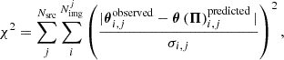
where Nsrc is the number of the background sources, Nimgj is the number of multiple images belonging to the jth source, and  and
and  are, respectively, the observed and model predicted position of the ith image of the jth source. The set of free parameters describing the mass distribution is represented by the vector Π. The uncertainty on the observed image positions is σi, j. Given the well-known limitation of parametric models (Johnson & Sharon 2016; Grillo et al. 2015) and additional deflections by line-of-sight massive perturbers (usually on the order of
  ; Jullo et al. 2010; Host 2012; Chirivì et al. 2018), we first assumed an uncertainty of
  to obtain the best-fit model and compare different mass parameterizations. For the sampling of the posterior distributions in Sect. 3.3, we rescaled σ in order to have a χ2/d.o.f. = 1, where d.o.f. is the number of degrees of freedom in each model.
We adopted different parameterizations for the cluster large-scale component and for the galaxy CMs. The former component dominates the mass budget of the cluster and accounts mainly for the dark matter halo (DMH). In this work, we used two commonly used parameterizations for this component in order to test which profile better reproduces the multiple image positions. The first model is the pseudo-isothermal elliptical mass distribution (PIEMD; Kassiola & Kovner 1993; Chirivì et al. 2018) with a core radius. In this parameterization, the lensing convergence is given by
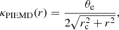
where θe is the Einstein radius, rc the core radius and r the radial coordinate that is constant over ellipses with r 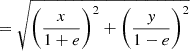 , and e being the ellipticity. In addition to these parameters, the orientation of the DMH is also free to vary and parameterized by θDMH, with respect to the x-axis and increasing clockwise. Thus, the total number of free parameters describing the PIEMD model is six. The second parameterization for the DMH is given by the Navarro-Frenk-White (NFW) model (Navarro et al. 1996). In this model, the spherical density profile and convergence are described in Golse & Kneib (2002) and Keeton (2002). The two free parameters are the characteristic density ρs, and the scale radius rs. The ellipticity in the NFW halo is implemented in the lens potential, following Halkola et al. (2006).
To account for the CMs, we parameterized the galaxies using the dual pseudo-isothermal elliptical mass distribution (dPIE; Elíasdóttir et al. 2007; Suyu & Halkola 2010). The lensing convergence for this model is given by
with truncation radius rt, and Einstein radius θe. The centroids of all CMs are fixed to the estimates obtained on the HST photometry using Source Extractor (SExtractor; Bertin & Arnouts 1996).
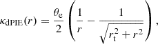
To reduce the number of free parameters describing the CMs, we adopted a mass-to-light scaling relation. One commonly used scaling is given by

This scaling relation is known as the tilt of fundamental plane (Dressler et al. 1987; Bender et al. 1992), where the total mass-to-light ratio increases with the luminosity as Mi/Li ∼ Li0.2. This relation is used to account for the systematic increase in the mass-to-light ratio relation observed in early-type galaxies and is shown to provide a better fit in cluster strong lensing studies (Grillo et al. 2015). We used the MAGAUTO parameter from SExtractor (Bertin & Arnouts 1996) in the HST filter F160W for the reference brightest cluster galaxy (BCG) magnitude, that is, 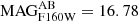 .
.
3.2. Best-fit parameterization
By assuming different lens models and varying the free parameters, we obtained the result shown in Table 3. In the first model, we only included the DMH. This simple model has only six free parameters but is capable of reproducing the positions of all multiple images with a relatively low δrms of  . In the next two models, the BCG is also taken into account, with both a circular and an elliptical symmetry. By introducing the BCG we can see a significant improvement in χ2. Furthermore, by adding the CMs to the next two models (following the scaling relations of Eq. (4)), the precision increases significantly without adding additional free parameters. For all PIEMD models, the axis ratio b/a of the DMH is about 0.3 (see, e.g., Table 4), which is very low for a mass distribution considering that we allowed the parameter range to be between 0.3 and 1. To investigate if this extreme axis ratio value is caused by an additional component not included in the model, we included an external shear component in the sixth and the seventh models (see Table 3). However, after including the shear in the model, the ellipticity of the DMH did not change and the best-fitting shear amplitude is very small (≈5 × 10⁻³). This suggest that the shear has no significant effect on the ellipticity of the DMH. Finally, we also tested a model with a NFW parameterization for the DMH to check how well a different model could fit the observed multiple images positions.
Table of the best-fit lens models.
Comparing two different models of the DMH (PIEMD and NFW).
To distinguish the goodness of different models, we used the Bayesian information criterion (BIC; Schwarz 1978) and the Akaike information criterion (AIC):

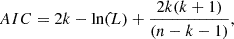
with the maximum likelihood  , the total number of free parameters k and the number of constraints n. Both quantities penalize models with an increased number of free parameters but with no significant improvements in the goodness of the fit. The model with the lowest BIC and AIC is chosen as a reference to avoid overfitting due to excessive freedom of the mass parameterization. Although model “DMHPIEMD” has the lowest AIC, it has the highest BIC value of the models in Table 3 and is an oversimplification of a cluster mass distribution because it does not account for the BCG and CMs (see, e.g., Grillo et al. 2015). On the other hand, the model “DMHPIEMD + BCGcir + CM” is favored by both BIC and AIC and we used this as our reference mass parameterization.
In Fig. 4 we show the critical curves for z = 3 for this best-fit model and the position of multiple images. It is worth noticing that the model with a NFW parameterization (DMHNFW + BCGcir + CM) has very similar BIC and AIC values, indicating that the two models are equivalent in terms of goodness of fit. However, in GLEE the ellipticity is introduced in the lens potential, and in cases of high ellipticity it gives unphysical convergency maps (Golse & Kneib 2002; Dúmet-Montoya et al. 2012), which is the case of our models (see Table 4 with small b/aDMH). Therefore, we adopted the PIEMD parameterization as the reference. The results of the NFW model are also presented in Table 4.
3.3. MCMC sampling
For the sampling runs of the favored model “DMHPIEMD+ BCGcir + CM”, we rescaled the positional errors in order to have χ2/d.o.f. = 1 and thus sensible confidence intervals for the values of the parameters. The value of the rescaled error is now 0.30″. With this, we accounted for effects that are not included in the modeling, such as the effect of line-of-sight perturbers (Jullo et al. 2010; Host 2012; Chirivì et al. 2018), and limitations of the parametric description. We let the Monte Carlo Markov chain (MCMC) run until the chain reached 2.5 × 10⁶ samples to ensure convergence. This MCMC method is based on the Metropolis–Hastings algorithm and provides the distribution and the uncertainties for the free parameters shown in Fig. 3 and Table 4. From the posterior distribution, we observe an offset of the x-coordinate of the DMH relative to the BCG center, and a strong and expected degeneracy between the quantities θe and rcore. In addition to this, the mass parameters of the DMH and BCG ( and
and  ) are anticorrelated in such a way that the total mass within the multiple image positions does not change (since this is the quantity that strong lensing robustly measures).
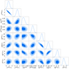 |
Fig. 3. Distribution of the DMHPIEMD + BCGcir + CM model. We see strong degeneracies in the xDMH-yDMH and |


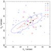 |
Fig. 4. Critical line (solid blue) and caustic (dashed red) of model DMHPIEMD + BCGcir + CM at source redshift z = 3. The positions of the lensed multiple images are indicated by circles, in seven different colors for the seven lensed background sources, as indicated in the legend. Open circles mark the images positions, and filled circles are the source positions. |
3.4. MACS J0035 total mass profile
To obtain the total mass profile, we randomly selected 100 models from the MCMC chain of the favored model “DMHPIEMD + BCGcir + CM”. For each of the 100 models, we generated using GLEE the two-dimensional convergence (κ) maps with a size of 120 arcsec per side, corresponding to ≈600 kpc at the cluster redshift. By summing up κ of each pixel in a circle centered around the BCG (at RA = 8.8588913, Dec = −20.2622861) with a certain radius r and multiplied with Σcrit and the area of the pixels, we obtained the total mass, M, as a function of r. In Fig. 5 we show the total cumulative mass as a function of radius r with the 68% confidence level uncertainties. Given the positions of multiple images, we obtained a precise measurement of the total mass in the region between 40 kpc and 200 kpc, which is reflected by the small error bars in this region.
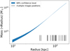 |
Fig. 5. Total radial mass distribution of MACS J0035. The range is from 101 to about 102 kpc. Since there are no multiple images in the inner core, our model cannot reconstruct the total mass in that area very well. The vertical segments in black indicate the locations of the lensed images. |
4. Conclusions
We performed a strong lensing analysis of the galaxy cluster MACS J0035 to constrain the mass parameter(s) of the cluster. We summarize our conclusions as follows:
-
By assuming fixed cosmological parameters, we could reconstruct the mass model of MACS J0035. We tested several mass distribution parameterizations and used the BIC and AIC to determine the reference model (see Table 3). The multiple images are located in the inner cluster core (< 35″), and our model can recover their positions with a
 .
. -
Our parametric model seems to have a large uncertainty when describing some parameters; in particular, the centroid of the DMH has an uncertainty of ± ∼ 1″ and the ellipticity is overestimated. This might be caused by an additional component not included in the model, and thus the mass distribution of the DMH may be more complex than we have assumed. Unfortunately, the number of strong lensing model constraints – 7 families and 21 multiple images in total – is not large enough to enable more freedom in the parameterization of the mass distribution.
-
The axis ratio b/a of the DMH predicted by our model is
 , which is extraordinarily low. This might be caused by an additional component not included in the model, and thus the mass distribution of the DMH might be more complex than we have assumed.
In conclusion, the strong gravitational lensing model presented in this study can be used to better understand the distant Universe. By applying this model to the MACS J0035 galaxy cluster, we have not only improved our knowledge of the cluster’s mass distribution and the magnification of background objects, but also identified several high-redshift objects that could provide valuable insights into the early stages of galaxy formation and evolution. This approach lays the groundwork for future observational work aimed at studying these high-z objects in greater detail, enhancing our understanding of the Universe’s expansion and the nature of dark matter and dark energy. Finally, the methodology developed here can be extended to other galaxy clusters, offering a framework for further cosmological studies
Data availability
The full version of Table 2 is available at the CDS via anonymous ftp to cdsarc.cds.unistra.fr (130.79.128.5) or via https://cdsarc.cds.unistra.fr/viz-bin/cat/J/A+A/698/A161
Final data products for the RELICS program are available at https://archive.stsci.edu/prepds/relics/
Acknowledgments
CS, GBC and SHS thank the Max Planck Society for support through the Max Planck Research Group and Max Planck Fellowship for SHS. This research is supported in part by the Excellence Cluster ORIGINS which is funded by the Deutsche Forschungsgemeinschaft (DFG, German Research Foundation) under Germany’s Excellence Strategy – EXC-2094 – 390783311.
References
- Adame, A. G., Aguilar, J., Ahlen, S., et al. 2025, JCAP, 2025, 021 [CrossRef] [Google Scholar]
- Astier, P., Guy, J., Regnault, N., et al. 2006, A&A, 447, 31 [NASA ADS] [CrossRef] [EDP Sciences] [Google Scholar]
- Bacon, R., Accardo, M., Adjali, L., et al. 2010, in Ground-based and Airborne Instrumentation for Astronomy III, eds. I. S. McLean, S. K. Ramsay, & H. Takami, SPIE Conf. Ser., 7735, 773508 [Google Scholar]
- Bender, R., Burstein, D., & Faber, S. 1992, ApJ, 399, 462 [NASA ADS] [CrossRef] [Google Scholar]
- Bertin, E., & Arnouts, S. 1996, A&AS, 117, 393 [NASA ADS] [CrossRef] [EDP Sciences] [Google Scholar]
- Caminha, G. B., Grillo, C., Rosati, P., et al. 2016, A&A, 587, A80 [NASA ADS] [CrossRef] [EDP Sciences] [Google Scholar]
- Caminha, G. B., Rosati, P., Grillo, C., et al. 2019, A&A, 632, A36 [NASA ADS] [CrossRef] [EDP Sciences] [Google Scholar]
- Caminha, G. B., Grillo, C., Rosati, P., et al. 2023, A&A, 678, A3 [NASA ADS] [CrossRef] [EDP Sciences] [Google Scholar]
- Chirivì, G., Suyu, S. H., Grillo, C., et al. 2018, A&A, 614, A8 [NASA ADS] [CrossRef] [EDP Sciences] [Google Scholar]
- Clowe, D., Bradač, M., Gonzalez, A. H., et al. 2006, ApJ, 648, L109 [NASA ADS] [CrossRef] [Google Scholar]
- Coe, D., Salmon, B., Bradač, M., et al. 2019, ApJ, 884, 85 [Google Scholar]
- DES Collaboration (Abbott, T. M. C., et al.) 2024, ApJ, 973, L14 [NASA ADS] [CrossRef] [Google Scholar]
- Dressler, A., Faber, S. M., Burstein, D., et al. 1987, ApJ, 313, L37 [CrossRef] [Google Scholar]
- Dúmet-Montoya, H. S., Caminha, G. B., & Makler, M. 2012, A&A, 544, A83 [NASA ADS] [CrossRef] [EDP Sciences] [Google Scholar]
- Ebeling, H., Edge, A. C., & Henry, J. P. 2001, ApJ, 553, 668 [Google Scholar]
- Eisenstein, D. J., Zehavi, I., Hogg, D. W., et al. 2005, ApJ, 633, 560 [Google Scholar]
- Elíasdóttir, A., Limousin, M., Richard, J., et al. 2007, arXiv e-prints [arXiv:0710.5636] [Google Scholar]
- Golse, G., & Kneib, J.-P. 2002, A&A, 390, 821 [NASA ADS] [CrossRef] [EDP Sciences] [Google Scholar]
- Grillo, C., Suyu, S. H., Rosati, P., et al. 2015, ApJ, 800, 38 [Google Scholar]
- Grillo, C., Rosati, P., Suyu, S. H., et al. 2020, ApJ, 898, 87 [Google Scholar]
- Grillo, C., Pagano, L., Rosati, P., & Suyu, S. H. 2024, A&A, 684, L23 [NASA ADS] [CrossRef] [EDP Sciences] [Google Scholar]
- Halkola, A., Seitz, S., & Pannella, M. 2006, MNRAS, 372, 1425 [Google Scholar]
- Hinshaw, G., Larson, D., Komatsu, E., et al. 2013, ApJS, 208, 19 [Google Scholar]
- Horesh, A., Maoz, D., Ebeling, H., Seidel, G., & Bartelmann, M. 2010, MNRAS, 406, 1318 [NASA ADS] [Google Scholar]
- Host, O. 2012, MNRAS, 420, L18 [NASA ADS] [CrossRef] [Google Scholar]
- Johnson, T. L., & Sharon, K. 2016, ApJ, 832, 82 [Google Scholar]
- Jullo, E., Natarajan, P., Kneib, J.-P., et al. 2010, Science, 329, 924 [CrossRef] [Google Scholar]
- Kassiola, A., & Kovner, I. 1993, ApJ, 417, 450 [Google Scholar]
- Keeton, C. R. 2002, arXiv e-prints [astro-ph/0102341] [Google Scholar]
- Kelly, P. L., Rodney, S., Treu, T., et al. 2023, Science, 380, abh1322 [CrossRef] [Google Scholar]
- Kneib, J.-P., & Natarajan, P. 2011, A&A Rev., 19, 47 [Google Scholar]
- Lotz, J. M., Koekemoer, A., Coe, D., et al. 2017, ApJ, 837, 97 [Google Scholar]
- Natarajan, P., Williams, L. L. R., Bradač, M., et al. 2024, Space Sci. Rev., 220, 19 [CrossRef] [Google Scholar]
- Navarro, J. F., Frenk, C. S., & White, S. D. M. 1996, ApJ, 462, 563 [Google Scholar]
- Oke, J. B. 1974, ApJS, 27, 21 [Google Scholar]
- Oke, J. B., & Gunn, J. E. 1983, ApJ, 266, 713 [NASA ADS] [CrossRef] [Google Scholar]
- Pascale, M., Frye, B. L., Pierel, J. D. R., et al. 2025, ApJ, 979, 13 [Google Scholar]
- Perlmutter, S., Aldering, G., Goldhaber, G., et al. 1999, ApJ, 517, 565 [Google Scholar]
- Planck Collaboration VI. 2020, A&A, 641, A6 [NASA ADS] [CrossRef] [EDP Sciences] [Google Scholar]
- Postman, M., Coe, D., Bení tez, N., et al. 2012, ApJS, 199, 25 [Google Scholar]
- Richard, J., Claeyssens, A., Lagattuta, D., et al. 2021, A&A, 646, A83 [EDP Sciences] [Google Scholar]
- Riess, A. G., Filippenko, A. V., Challis, P., et al. 1998, AJ, 116, 1009 [Google Scholar]
- Rosati, P., Balestra, I., Grillo, C., et al. 2014, The Messenger, 158, 48 [NASA ADS] [Google Scholar]
- Rubin, D., Aldering, G., Betoule, M., et al. 2025, AAS, 245, 250.02 [Google Scholar]
- Schwarz, G. 1978, Ann. Stat., 6, 461 [Google Scholar]
- Scolnic, D., Brout, D., Carr, A., et al. 2022, ApJ, 938, 113 [NASA ADS] [CrossRef] [Google Scholar]
- Sevilla-Noarbe, I., Bechtol, K., Kind, M. C., et al. 2021, ApJS, 254, 24 [NASA ADS] [CrossRef] [Google Scholar]
- Smoot, G. F., Bennett, C. L., Kogut, A., et al. 1992, ApJ, 396, L1 [Google Scholar]
- Soto, K. T., Lilly, S. J., Bacon, R., Richard, J., & Conseil, S. 2016, MNRAS, 458, 3210 [Google Scholar]
- Suyu, S. H., & Halkola, A. 2010, A&A, 524, A94 [NASA ADS] [CrossRef] [EDP Sciences] [Google Scholar]
- Suyu, S. H., Hensel, S. W., McKean, J. P., et al. 2012, ApJ, 750, 10 [Google Scholar]
- Suzuki, N., Rubin, D., Lidman, C., et al. 2012, ApJ, 746, 85 [NASA ADS] [CrossRef] [Google Scholar]
- Tyson, J. A., Valdes, F., & Wenk, R. A. 1990, ApJ, 349, L1 [CrossRef] [Google Scholar]
- Vega-Ferrero, J., Diego, J. M., Miranda, V., & Bernstein, G. M. 2018, ApJ, 853, L31 [NASA ADS] [CrossRef] [Google Scholar]
- Verde, L., Heavens, A. F., Percival, W. J., et al. 2002, MNRAS, 335, 432 [NASA ADS] [CrossRef] [Google Scholar]
- Weilbacher, P. M., Streicher, O., & Palsa, R. 2016, MUSE-DRP: MUSE Data Reduction Pipeline, Astrophysics Source Code Library [record ascl:1610.004] [Google Scholar]
- Weilbacher, P. M., Palsa, R., Streicher, O., et al. 2020, A&A, 641, A28 [NASA ADS] [CrossRef] [EDP Sciences] [Google Scholar]
All Tables
All Figures
|
Fig. 1. Galaxy cluster MACS J0035 with a redshift of zL = 0.3529 at RA: 8.8588913, Dec: −20.2622861 (the coordinates mark the center of the BCG). This image includes 21 multiple images from 7 different sources, all highlighted in yellow. Diamonds indicate CMs with spectroscopic confirmation and selected from the photometry, in cyan and magenta, respectively. The BCG is marked with a blue circle. Red circles indicate multiple images with no secure spectroscopic redshift but belonging to secure families. |
| In the text | |
|
Fig. 2. Spectra of multiply lensed sources. Blue lines indicate the spectroscopic data and gray regions of variance. Vertical lines show the main spectral features present in each wavelength range. In cases where the continuum is clearly detected, the red line corresponds to the template used to estimate the exact redshift. The small HST cutouts in the top-left region of each panel are 2 arcsec per side. |
| In the text | |
|
Fig. 3. Distribution of the DMHPIEMD + BCGcir + CM model. We see strong degeneracies in the xDMH-yDMH and |
| In the text | |
|
Fig. 4. Critical line (solid blue) and caustic (dashed red) of model DMHPIEMD + BCGcir + CM at source redshift z = 3. The positions of the lensed multiple images are indicated by circles, in seven different colors for the seven lensed background sources, as indicated in the legend. Open circles mark the images positions, and filled circles are the source positions. |
| In the text | |
|
Fig. 5. Total radial mass distribution of MACS J0035. The range is from 101 to about 102 kpc. Since there are no multiple images in the inner core, our model cannot reconstruct the total mass in that area very well. The vertical segments in black indicate the locations of the lensed images. |
| In the text | |
Current usage metrics show cumulative count of Article Views (full-text article views including HTML views, PDF and ePub downloads, according to the available data) and Abstracts Views on Vision4Press platform.
Data correspond to usage on the plateform after 2015. The current usage metrics is available 48-96 hours after online publication and is updated daily on week days.
Initial download of the metrics may take a while.