| Issue |
A&A
Volume 627, July 2019
|
|
|---|---|---|
| Article Number | A84 | |
| Number of page(s) | 21 | |
| Section | Cosmology (including clusters of galaxies) | |
| DOI | https://doi.org/10.1051/0004-6361/201833645 | |
| Published online | 04 July 2019 | |
Lyman α-emitting galaxies in the epoch of reionization
1
Institute of Theoretical Astrophysics, University of Oslo, PO Box 1029 Blindern, 0315 Oslo, Norway
e-mail: This email address is being protected from spambots. You need JavaScript enabled to view it.
2
Cosmic Dawn Center (DAWN), Denmark
3
Dark Cosmology Centre, Niels Bohr Institute, University of Copenhagen, Juliane Maries Vej 30, 2100 Copenhagen Ø, Denmark
4
Marie Kruses Skole, Stavnsholtvej 29-31, 3520 Farum, Denmark
5
Niels Bohr Institute, University of Copenhagen, Lyngbyvej 2, 2100 Copenhagen Ø, Denmark
6
WestGrid, Vancouver, BC, Canada
Received:
14
June
2018
Accepted:
8
April
2019
Abstract
With a total integration time of 168 h and a narrowband filter tuned to Lyα emission from z = 8.8, the UltraVISTA survey has set out to find some of the most distant galaxies, on the verge of the epoch of reionization. Previous calculations of the expected number of detected Lyα-emitting galaxies (LAEs) at this redshift based for example on extrapolation of lower-redshift luminosity functions did not explicitly take into account the radiative transfer of Lyα. In this work we have combined a theoretical model for the halo mass function, that is, the expected number of haloes per volume, with numerical results from high-resolution cosmological hydro-simulations post-processed with radiative transfer of ionizing UV and Lyα radiation, assessing the visibility of LAEs residing in these haloes. We have taken into account uncertainties such as cosmic variance and the anisotropic escape of Lyα, and predict that once the survey has finished, the probabilities of detecting none, one, or more than one are roughly 90%, 10%, and 1%, respectively. This is a significantly smaller success rate than in earlier predictions, due to the combined effect of a highly neutral intergalactic medium (IGM) scattering Lyα to such large distances from the galaxy that they fall outside the observational aperture, and to the actual depth of the survey being less than predicted. Because the IGM affects narrowband (NB) and broadband (BB) magnitudes differently, we argue for a relaxed colour selection criterion of mNB − mBB ≃ +0.85 in the AB system. Since the flux is dominated by the continuum, however, even if a galaxy is detectable in the NB, its probability of being selected as a narrowband excess object is ≲35%. Various additional properties of galaxies at this redshift are predicted, for example, the Lyα and UV luminosity functions, the stellar mass–halo mass relation, the spectral shape, the optimal aperture, as well as the anisotropic escape of Lyα through both the dusty, interstellar medium and through the partly neutral IGM. Finally, we describe and make public a fast numerical code for adding numbers with asymmetric uncertainties (“x+σ+−σ−”) which proves significantly more precise than the standard, but wrong, way of separately adding upper and lower uncertainties in quadrature.
Key words: radiative transfer / galaxies: high-redshift / dark ages / reionization / first stars
Deceased 9.6.2018.
© ESO 2019
1. Introduction
Unveiling the evolution and the constituents of the early Universe is as exciting and important as it is arduous. While the formation of structure from primordial fluctuations to massive haloes can be accounted for purely by gravitational collapse of matter, the mechanisms that lead to the emission of light – the primary way of gaining information from the high-redshift Universe – are less clear. The first generation of stars seems to have emerged some 200 Myr after the Big Bang (Barkana & Loeb 2001; Visbal et al. 2012; Bowman et al. 2018). In a virtually neutral Universe, the escape of ionizing radiation was inhibited, but eventually the Universe was reionized and galaxies became more easily detectable.
Hard UV radiation is emitted from the most massive and hence hot stars of a starburst, attempts to escape the surrounding neutral gas, and carves out bubbles of ionized hydrogen in the interstellar medium (ISM). Because of the high densities involved during the epoch of reionization (EoR), recombination happens on very short timescales, eventually reprocessing a third of the radiation bluewards of 912 Å into a single emission line – the Lyα line at 1216 Å. Consequently, up to 10% of the total, bolometric luminosity can be emitted in Lyα, as first predicted by Partridge & Peebles (1967). At high redshifts, where the metallicity may be expected to be substantially lower and the initial mass function (IMF) may be more top-heavy than the Salpeter (1955) IMF assumed by Partridge & Peebles (1967), the fraction may be even higher, up to 20–40% (Raiter et al. 2010). This fortunate fact facilitates observations of galaxies that would otherwise be impossible to detect. In addition to the Lyα precipitated by stars, a notable amount is surmised to be emitted from cooling radiation following the cold accretion of gas onto the galaxies (see discussion in Sect. 3.3.2).
When the UltraVISTA survey (discussed in detail below) set out, the most distant known galaxy was the Iye et al. (2006) Lyα emitter (LAE) at z = 6.96, which held its record for five years. Eventually, a few LAEs at redshifts beyond 7 were reported (e.g. Vanzella et al. 2011; Shibuya et al. 2012; Finkelstein et al. 2013), and more recently, galaxies at z = 8.68 (Zitrin et al. 2015), z = 11.09 (Oesch et al. 2016), and z = 9.1 (Hashimoto et al. 2018) were detected, showing that the survey should at least have a chance of detecting LAEs at z = 8.8. The galaxy detected by Oesch et al. (2016) was detected due to the Lyα break rather than the line, while the one found by Hashimoto et al. (2018) was detected in O III albeit with tentative evidence for a Lyα line; thus, an UltraVISTA-detection at z = 8.8 could be the highest-redshift LAE to date.
Detecting the most distant astronomical object has long been a goal in itself, but pushing such observations to the limit is not just a question of increasing the volume of the explored part of the Universe, or breaking a record. Although the difference in lookback time between, for example, z = 8 and 9 is merely a hundred Myr, this is a significant fraction of the age of the Universe at this time, which was only half a Gyr. Thus, these extreme observations offer crucial insights into the timescales of the formation, evolution, and general properties of galaxies and the intergalactic medium (IGM). Moreover, the number density and clustering of LAEs at z > 6 can put constraints on reionization (Furlanetto et al. 2006; McQuinn et al. 2007; Iliev et al. 2008; Jensen et al. 2013). As yet, quantifying the clustering of LAEs has been rather inadequate due to limited sample sizes, but at these redshifts even the detection of a single galaxy provides important constraints.
Commissioning of the 4.1 m survey telescope VISTA, located close to the VLT on a neighbouring peak, and its wide-field infrared camera VIRCAM (Sutherland et al. 2014) was completed in 2009. VISTA is used mainly for large, multi-year, public surveys (Arnaboldi et al. 2017). One of these is UltraVISTA (McCracken et al. 2012), which utilizes the VISTA telescope to obtain deep imaging of 1.2 × 1.5 deg2 of the COSMOS field (Scoville et al. 2007) in the four near-IR filters Y, J, H and Ks. Half of this field, the four so-called ultra-deep stripes covering about 1 deg2, are also observed in a narrowband (NB) filter NB118 centred at 1.19 μm (Milvang-Jensen et al. 2013), corresponding to Lyα redshifted from z = 8.8, or less than 600 Myr after the Big Bang. This wavelength was chosen to be relatively free of airglow emission. Unfortunately the filter turned out to be subject to a small shift in wavelength of approximately 3.5 nm when mounted in VIRCAM, which, while still effectively probing the same redshift, is large enough that airglow lines are partly entered, resulting in a somewhat lower sensitivity (Milvang-Jensen et al. 2013).
The NB survey, which constitutes ∼10% of the full UltraVISTA survey, set out in December 2009 to construct an ultra-deep image from 168 h of integration. An original 5σ detection limit of F = 3.7 × 10⁻¹⁸ erg s−1 cm−2 (corresponding to an AB magnitude of 26.0) was expected (Nilsson et al. 2007); however, due to the above-mentioned shift, as well as a too-optimistic sky background assumed by the ESO Exposure Time Calculator used at the time, it turned out to be somewhat shallower. Based on the GTO data (Milvang-Jensen et al. 2013), the detection limit for the final UltraVISTA is predicted to be F = 1.5–1.7 × 10⁻¹⁷ erg s−1 cm−2 (see e.g. Matthee et al. 2014). The depth and the large area still results in a much larger volume than in previous surveys.
The observational part of the NB survey was completed in 2018. Since the data reduction is extremely time-consuming, the latest data release (DR3) only contains 60% of the final NB exposure; so far there is no sign of the detection of z = 8.8 LAEs. To determine if we can hope to detect any at all, we must estimate the luminosity function (LF) of LAEs at a hitherto unexplored epoch of the history of the Universe. In essence, there are two complementary approaches to address this problem; one can look at LFs of galaxies probed at lower redshift, and then extrapolate to z = 8.8, assuming a model for the evolution of both galaxies and the IGM. Alternatively, one may resort to numerical simulations, relying on the faith in our understanding of the physics governing the formation of structure.
Prior to the launch of UltraVISTA, Nilsson et al. (2007) made predictions for the expected number of detected LAEs at z = 8.8. At this time, realistic Lyα radiative transfer (RT) was in its infancy and unavailable to most astronomers. Instead these authors followed three different approaches: Model 1 used the semi-analytical galaxy formation model GALFORM (Cole et al. 2000) with a common Lyα escape fraction of fesc = 0.02 or 0.2 for galaxies of all masses, to match LF observations at lower redshifts (Le Delliou et al. 2006). Model 2 uses the phenomenological model of Thommes & Meisenheimer (2005), normalized to match the observed mass function of galaxy spheroids at z = 0. Model 3 uses a Schechter (1976) LF with parameters extrapolated linearly from fits at 3.1 ≤ z ≤ 6.5. The three models predict between three and 20 detections.
With similar extrapolations of lower-redshift LFs, Faisst et al. (2014) predicted a less optimistic 0.6 ± 0.3, while Matthee et al. (2014, see below) predicted, with their most optimistic LF, a number of ≲23. However, using the Nilsson et al. (2007) LF extrapolation, but with realistically estimated depth, predicts only 0.19.
Observations of LAEs at z = 8.8 have been attempted before. Willis & Courbin (2005) uses the VLT/ISAAC narrowband to sample a volume of 340 h−3 cMpc3 to a limiting flux of 3.28 × 10⁻¹⁸ erg s−1 cm−2, while Cuby et al. (2007), using the same instrument, chooses a larger area of 31 arcmin2 albeit to a shallower threshold of ∼1.3 × 10⁻¹⁷ erg s−1 cm−2. Taking advantage of the lensing effect of three clusters, Willis et al. (2008) reaches 3.7 × 10⁻¹⁸ in an area of 12 arcmin2. Sobral et al. (2009) surveyed 1.4 deg2 down to ∼7.6 × 10⁻¹⁷ erg s−1 cm−2 with UKIRT/WFCam in the HizELS survey at z ≃ 9, and Matthee et al. (2014) searches the hitherto largest area of 10 deg2 with CFHT/WIRCam and VLT/SINFONI followup down to 7 × 10⁻¹⁷ erg s−1 cm−2. However, all surveys returned null-results.
Numerically predicting the expected number of observed galaxies is a challenging task, but can essentially be divided into two sub-projects. First, calculating the number of galaxies in the cosmic volume surveyed by UltraVISTA, and second, calculating the observability of those galaxies. In principle, everything could be computed in a single numerical simulation calculating the galaxy formation and emission of light from the galaxies. In practise, however, the simultaneous needs for a large volume and high resolution obliges us to split up the project into several parts. In the following, the various parts of the project are outlined.
Galaxies reside in dark matter haloes, the number density of which is given by the halo mass function (HMF) which can be estimated analytically or determined via large cosmological simulations, or using a combination hereof. Whether or not a given halo hosts a galaxy is given by a halo occupation distribution, which is defined once the concept of a galaxy is defined. The easiest approach is to simply define a galaxy as any conglomerate of baryons, or even any dark matter (DM) halo, whether or not these particles have made themselves visible by producing any kind of luminous matter. Subsequently we can then ask the question “Is a given galaxy observable?”
Simulating galaxy formation realistically requires not only inclusion of hydrodynamics, but also higher resolution than that offered by large-scale simulations. Moreover, for the RT markedly higher resolution is needed, making it impossible to simulate a statistically robust sample of galaxies with sufficient resolution. These difficulties are dealt with by carrying out a fully cosmological, hydrodynamical, but medium-sized, simulation that is large enough for the interaction between individual galaxies to be accounted for. Subsequently, a number of galaxies are extracted from the simulation, and resimulated at higher resolution. Several different models for star formation and feedback are investigated.
Finally, two RT schemes are employed: While the cosmological simulation uses an on-the-fly approximation of the ionizing UV background (UVB), a full Lyman continuum (LyC) RT is performed on the extracted galaxies and their environments, after which the Lyα RT is conducted, monitoring the spatial and spectral distribution of the photons that reach the observer, that is, those which are not absorbed by dust, or scattered out of the line of sight (LOS) by the IGM.
The two sub-projects – calculating the number density and the observability – are described in Sects. 2 and 3, respectively. The results are presented in Sect. 4, discussed in Sect. 5, and summarized in Sect. 6.
2. Galaxy number density
2.1. Halo mass function
The problem of calculating the distribution of the masses Mh of collapsed haloes was addressed first by Press & Schechter (1974; hereafter PS), who considered the spherical collapse of gravitationally interacting matter from an initial, smoothed density field. The resulting HMF expressed as number density per logarithmic mass bin can be written as
 (1)
(1)
where ρM, 0 is the present-day average mass density of the Universe, σ(Mh, z) is the rms fluctuations of the density field smoothed with a top-hat filter W(R) of radius R = (3Mh/4πρM(z))1/3, and f(σ) is discussed below.
For a linearly extrapolated density field characterized by a power spectrum P(k), the rms fluctuation is given by
 (2)
(2)
where  is the Fourier transform of the real-space filter1W(R), and δ(z)=D(z)/D(0) is the linear growth rate normalized to unity today. The growth rate function, in turn, involves an integral over the expansion history, but is very well approximated (Lahav et al. 1991; Carroll et al. 1992) by
 (3)
(3)
The last term in Eq. (1), f(σ), is the multiplicity function giving the mass fraction associated with halos in a unit range of lnν, with ν ≡ δcr/σ and δcr ≃ 1.686 the critical density contrast needed for gravitational collapse. Only in the PS formalism is it possible to obtain an analytical form of f(σ); in general it must be empirically derived by fitting to halo abundances in cosmological simulations. The PS HMF gave good fits to simulations at that time, but as computing resources improved, it was found numerically that it over- (under-) predicts the collapsed fraction at the low- (high-) mass end (e.g. Governato et al. 1999).
By introducing two extra parameters, Sheth & Tormen (1999; hereafter ST) gave an improved formalism (further detailed in Sheth et al. 2001 and Sheth & Tormen 2002), allowing for ellipsoidal structures to form. In the ST formalism the multiplicity function is given by
![Mathematical equation: $$ \begin{aligned} f(\sigma ) = A \sqrt{\frac{2\tilde{\nu }}{\pi }} \left[ 1 + \tilde{\nu }^{-p} \right] \mathrm{e}^{-\tilde{\nu }/2}, \end{aligned} $$](/articles/aa/full_html/2019/07/aa33645-18/aa33645-18-eq6.gif) (4)
(4)
where A ≃ 0.322 is a normalization constant,  with a = 0.707 describing a high-mass cutoff in an N-body simulation, and p = 0.3 is given by the shape of the HMF at low masses in the simulation. The PS HMF is recovered using
  .
.
While the ST HMF is much more accurate, especially at low redshifts, it still tends to overpredict the abundance of haloes at higher redshifts, when comparing to large, cosmological simulations. On the basis of the so-called Bolshoi simulation – an 8.5 billion particle simulation of comoving volume (250 h−1 Mpc)3 – Klypin et al. (2011) provide a simple z-dependent correction factor which brings the analytical predictions much closer to the results of the simulation:
![Mathematical equation: $$ \begin{aligned} F(z) = \frac{[5.501\delta (z)]^4}{1 + [5.500\delta (z)]^4}\cdot \end{aligned} $$](/articles/aa/full_html/2019/07/aa33645-18/aa33645-18-eq9.gif) (5)
(5)
The Bolshoi simulation uses a (near-)WMAP seven-year data cosmology (Jarosik et al. 2011). For our analysis we have adopted the ST HMF with the correction factor in Eq. (5); in Sect. 5.2 we discuss the implications of using other HMFs and the more recent Planck cosmology (Ade et al. 2016).
2.2. UltraVISTA area and depth
To get the total number of galaxies, the number density must be multiplied by the volume surveyed by UltraVISTA. However, not all parts of the area are equally exposed. VIRCAM comprises 16 detectors (each with its own NB118 filter), which cannot be placed adjacently but instead are separated by a large fraction of a detector size. To acquire a contiguous image, the camera is shifted in the declination direction between exposures (or “paw prints”), resulting in most of the area being exposed twice, while the top and bottom 5.5′ are exposed just once, in units of a single paw print exposure time. With a final, total exposure time of 168 h, split equally in the three paw prints, most of the area will reach an exposure time of 112 h. Moreover, detector #16 and, to a lesser extent, #4 have sizable unreliable regions, which are excluded from the analysis. The result is that various parts of the area is sensitive to different depths. For details on exposures2. The total (non-dead) area exposed at least once is 1.07 deg2, which at z = 8.8 corresponds to 150 h−2 Mpc2, or 14.5 × 10³ h−2 cMpc2.
The depth of the volume is also not unequivocal; since the transmission curves of the filters are not tophats, different observed wavelengths, and hence different distances, are probed to different depths. Moreover, the 16 filters are slightly different, and have slightly different central wavelengths. In general, they all have roughly “full” transmission (i.e. around 60%) in a window of ∼70 Å. Outside of this region the transmission tapers off in such a way that the average FWHM is 123 ± 3 Å. If the emission lines were delta functions, at z = 8.8 this would translate into galaxies within a slab of 19 h−1 cMpc thick being detected. Since resonant scattering in fact broadens the emission lines by several Ångströms (in the rest frame), galaxies on the edges of this slab are less conspicuous than more centrally located ones. For an extensive description of the filters and transmission curves, see Milvang-Jensen et al. (2013).
The consequence is that the exact volume becomes a function of the flux limit of the observation; whereas a faint galaxy may only be detected if it lies at the centre of a filter, a bright galaxy may be detected even if it lies in the wing. Thus, any survey probes bright galaxies in a larger volume than fainter ones. An approximate volume can be computed from the average filter FWHM and the area exposed at least once; this estimate yields 290 h−3 Mpc3, or 2.7 × 10⁵ h−3 cMpc3.
Likewise, line broadening from RT effects may make galaxies both more and less visible: a Lyα line that would be detectable if it were a delta-like line can be smeared out over tens of Ångströms (in the observer’s frame), lowering the flux density below the sensitivity threshold. On the other hand, a (bright) line lying so far out in the wing of the filter that it would be undetectable as a delta-line, could be broadened into the sensitive part of the filter.
To address these complications, in the following calculations we integrate the simulated spectra over the exact filter shapes for each of the 16 filters. Additionally, we split the UltraVISTA NB118 image up in 52 regions with individual limiting magnitudes, corresponding to the regions that are exposed once or twice with different detectors3.
3. Galaxy observability
Whether or not a galaxy is observable depends on many factors, from its formation history, to its ability to create luminous objects, to the emitted light making its way out through the galaxy and down to us. To simulate this numerically requires detailed modelling; in particular, high resolution and a realistic H I field is needed for the Lyα RT. In the following, the simulations of the galaxies and the RT is described.
3.1. Cosmological hydro-simulations
3.1.1. The code
The galaxies were simulated using smoothed particle hydrodynamics (SPH). The TreeSPH type code Hernquist & Katz (1989) used to simulate the formation and evolution of galaxies to z = 8.8 is in most aspects identical to the code described by Sommer-Larsen & Fynbo (2017). In particular, the superwind prescription for starburst-driven energy feedback was implemented, and a Chabrier (2003) IMF is employed. This enables the continuing formation of starburst-driven (metal-enriched) outflows (discussed further in Sect. 5.5), in line with indications of recent observations of O VI and O VII absorption in the Galactic CGM. Such outflows are also of great significance to the Lyα RT (see Sect. 5.5), especially during the EoR (Dijkstra & Wyithe 2010; Dijkstra et al. 2011). The code used for the present work differs from the one described in Sommer-Larsen & Fynbo (2017) in a few aspects: (1) a “stretched” version of the Haardt & Madau (1996) UVB was used, rather than the Haardt & Madau (2012) UVB – the stretched UVB turns on at z = 12, whereas the original Haardt & Madau (1996) UVB turns on at z = 6 (see Laursen et al. 2011 for more detail), (2) early stellar feedback (ESF) was not implemented in the simulations described in this work, and (3) the effects of self-shielding of the UVB by gas is not described using the mean field approximation of Rahmati et al. (2013). Instead we assume that the UVB is fully shielded in regions where the mean free path of Lyman limit photons is less than 0.1 kpc.
3.1.2. Simulations
One expects the brightest and most Lyα-luminous galaxies observable at z = 8.8 to be located in higher-density, proto-cluster regions of the Universe. Hence, emphasis is placed on simulating such regions at high resolution. To this end, the well-known “zoom-in” technique (e.g. Navarro & White 1994; Oñorbe et al. 2013) is applied in two steps, as detailed in the following.
First, a low resolution, DM-only simulation is run to z = 0, using 1283 particles in a (150 h−1 cMpc)3 box with periodic boundary conditions, and starting at zi = 39. The cosmological parameters of the simulation (and the subsequent simulations described below) are {ΩM, ΩΛ, h, n, σ8} = {0.3, 0.7, 0.7,0.95, 0.9}. This is somewhat different from the cosmology of the HMF, but we will only use these simulations to assess the link between DM and baryons, and moreover, unless otherwise stated, factor out the h-dependence from cosmological quantities.
Two of the most massive DM haloes, at z = 0, are selected for re-simulation using the zoom-in technique; they correspond in several aspects to the Virgo and (sub-)Coma clusters, with virial masses at z = 0 of about 3 × 10¹⁴ and 1.2 × 10¹⁵ M⊙ and “temperatures” of kT ∼ 3 and 6 keV, respectively (see Sommer-Larsen et al. 2005; Romeo et al. 2006 for more detail). For each cluster, all DM particles within the virial radius at z = 0 have been traced back to the initial conditions at zi. The particles are contained within “virial volumes” having a linear extent of 20 − 30 h−1 cMpc, and within these volumes the numerical resolution is increased by 512 times in mass, and eight times in linear resolution. In addition, each higher resolution DM particle is split into a gas particle and a DM particle – a baryonic fraction fb = mSPH/(mDM + mSPH)=0.15 is assumed, in quite good agreement with recent values reported by the WMAP and Planck collaborations.
The mass resolution reached inside the resampled Lagrangian sub-volumes is mDM = 2.2 × 10⁸ h−1 M⊙ and mSPH = m⋆ = 3.9 × 10⁷ h−1 M⊙. Using the code described in Sect. 3.1.1, the evolution of the two virial volumes and the lower-resolution regions around these is then simulated from zi = 39 to z = 8.8. The gravity softening lengths ϵ are kept fixed in comoving coordinates until a redshift of 15, and at later times they are constant in physical coordinates. In the higher-resolution regions, at z < 15, ϵSPH = ϵ⋆ = 0.75 h−1 kpc and ϵDM = 1.3 h−1 kpc.
At z = 8.8, 20 galaxies of stellar mass M⋆ ≳ 3 × 10⁸ M⊙, corresponding to an absolute UV magnitude at 1600 Å of MUV ≲ −20 (see Fig. 4), are selected from the two simulations. The galaxies are identified in the higher-resolution regions of the two proto-cluster simulations using the algorithm described, for example, in Sommer-Larsen et al. (2005). For each of the 20 galaxies, the DM particles inside of the virial radius (at z = 8.8) are traced back to the initial conditions at zi of the two resolution-increased proto-cluster simulations described above. It is found that, in each case, this virial volume is contained within a sphere of radius 3 h−1 cMpc. For each galaxy, the numerical resolution in this sphere (located within the higher-resolution region of the corresponding proto-cluster initial conditions) is additionally increased by 64 times in mass, and four times in linear resolution. Consequently, the mass resolution reached inside these re-sampled spheres is mDM = 3.4 × 10⁶ h−1 M⊙ and mSPH = m⋆ = 6.1 × 10⁵ h−1 M⊙.
The 20 sets of nested, twice resolution-increased initial conditions form the base of the “production” simulations presented in this work. For each of the 20 sets, the code described in Sect. 3.1.1 was used to simulate the evolution of the formation region of a fairly massive galaxy, from zi = 39 to z = 8.8. For computational reasons, the 20 high-resolution (HR) regions were not evolved at the same time as one simulation, but were rather simulated one-by-one, resulting in a total of 20 production simulations. At z < 15, ϵSPH = ϵ⋆ = 188 h−1 pc and ϵDM = 335 h−1 pc in the HR regions. The minimum smoothing length is lmin = 10 h−1 pc. At z = 8.8, the HR regions reach out to distances of about 150 kpc (physical) from the central galaxies. The virial radii of the central galaxies range from 12–25 kpc, so the HR regions around the galaxies stretch 6–12 times as far as the virial radius. Consequently, other (typically smaller) galaxies are also present in these 20 simulations. Using the galaxy detection algorithm referred to above, a total of about 500 galaxies are identified – most of the analysis presented in this work builds on this sample of simulated galaxies.
In addition to the 20 simulations discussed above, for convergence study purposes, seven of the 20 galaxies were also simulated at a mass resolution eight times higher, and a linear resolution that was twice as high. The initial conditions for these seven simulations were constructed in the same way as described above, except that (for computational purposes) each galaxy was represented by a radius 1 h−1 cMpc sphere in the initial conditions (rather than the radius 3 h−1 cMpc spheres described above), in which the mass resolution is increased by 512 times (rather than the 64× above), and the linear resolution was increased by a factor of eight (rather than the factor of four above). The seven simulations were then run from zi = 39 to z = 8.8. The mass resolution reached inside these re-sampled spheres is, consequently, mDM = 4.3 × 10⁵ h−1 M⊙ and mSPH = m⋆ = 7.6 × 10⁴ h−1 M⊙. Moreover, at z < 15, ϵSPH = ϵ⋆ = 94 and ϵDM = 167 h−1 pc in the (ultra-)HR regions. At z = 8.8, the HR regions only reach out to a couple of virial radii from the central galaxies, but the simulations can nevertheless be used for some aspects of convergence studies, detailed in Appendix A.
3.2. Ionizing UV radiative transfer
As described above, the hydro-simulations employ an approximate scheme for the RT of ionizing UV radiation. Beginning at zre = 12, a UVB field similar in shape to Haardt & Madau (1996) is assumed to build up, exposing all regions characterized by a Lyman-limit photon mean free path greater than 0.1 kpc fully to the field, while the remaining regions are assumed to be self-shielded. This results in roughly half of the hydrogen by mass in the simulation being ionized at z ∼ 10–11, consistent with what is inferred from WMAP polarization maps (Bennett et al. 2013, zre = 10.6 ± 1.0), the cosmological parameters of which our simulation is quite close to, but ∼100 Myr earlier than the more recent result by Ade et al. (2016,  ). The implications of this are discussed in Sect. 5.2.
To model the local LyC coming from stars in the galaxy, we post-processed the snapshots at z = 8.8 with a detailed LyC RT scheme. The physical properties of the SPH particles are first interpolated onto an adaptively refined grid of base resolution 1283, with up to 15 additional levels of refinement, such that no cell contains more than one particle. The smallest cells thus have a linear extent 20 h−1 Mpc/(1 + 8.8)/128/215 ≃ 0.5 h−1 pc, although the “true” resolution of our hydro-simulations is given by the minimum smoothing length lmin = 10 h−1 pc. The same adaptive mesh refinement (AMR) was used in the subsequent Lyα RT. At each stellar source in the simulation twelve rays are “emitted”, covering all 4π directions isotropically. As one moves further away from the source, or enters refined cells, these rays are then split recursively into four rays each to maintain adequate resolution (at least several ray segments per every cell in the volume). Along the rays, the equlibrium photoionization state of each cell is calculated iteratively, taking into account both transfer of stellar LyC photons and the above-mentioned UVB. The stellar LyC RT was computed separately in the frequency bands [13.6, 24.6] eV, [24.6, 54.4] eV, and [54.4, ∞] eV. For details, see Razoumov & Sommer-Larsen (2006, 2007).
3.3. Lyα radiative transfer
3.3.1. Galactic radiative transfer
To conduct the Lyα RT we used the code MOCALATA (Laursen et al. 2009a,b). MOCALATA is a ray-tracing Monte Carlo code that operates on an AMR grid, so we used the same grid that was constructed for the LyC RT. Similar codes have previously been applied to both cosmological simulations (e.g. Tasitsiomi 2006; Zheng et al. 2010; Kollmeier et al. 2010; Barnes et al. 2011; Trebitsch et al. 2016) and in idealized model galaxies (e.g. Zheng & Miralda-Escude 2002; Verhamme et al. 2006; Dijkstra et al. 2006; Gronke & Dijkstra 2014). We briefly outline the characteristics of the code below:
Each cell contains the physical variables that are important for the RT, which are Lyα and continuum emissivity LLyα and LFUV, gas temperature T, velocity field vbulk, as well as densities nH I and nd of neutral hydrogen and dust. Lyα emissivity is calculated as the sum of Lyα photons produced from recombinations following ionization (mainly from hot stars, but also from the UVB field) and decays following collisions of neutral atoms with electrons; so-called cooling radiation, discussed in more detail in the next section. That is, the total Lyα emissivity (in erg s−1 cm−3) is
 (6)
(6)
where ne and nH II are the electron and proton densities, respectively, hν0 = 10.2 eV is the energy of a Lyα photon, and
 (7)
(7)
with T4 ≡ T/104 K is the probability of a recombination resulting in a Lyα photon (Pengelly & Seaton 1964; Martin 1988; Cantalupo et al. 2008). Furthermore,
![Mathematical equation: $$ \begin{aligned} \alpha _{\rm {B}} = 2.753\times 10^{-14}\,\mathrm{cm} ^3\,\mathrm{s} ^{-1}\, \frac{\lambda _{{\text{ H}} {\text{ II}}}^{1.500}}{[1 + (\lambda _{{\text{ H}} {\text{ II}}}/2.740)^{0.407}]^{2.242}} \end{aligned} $$](/articles/aa/full_html/2019/07/aa33645-18/aa33645-18-eq13.gif) (8)
(8)
with λH II ≡ 2 × 157 807 K/T is the case B recombination coefficient (Hui & Gnedin 1997), and
 (9)
(9)
with kB the Boltzmann constant is the collisional excitation rate coefficient (Callaway et al. 1987; Goerdt et al. 2010).
Individual photons are emitted from a given cell with a probability proportional to the emissivity in that cell, in a random direction, and is followed as it scatters stochastically on the neutral hydrogen out through the ISM, until it either escapes the galaxy or is absorbed by dust. The galaxy is “observed” from six different directions, thus providing a measure of the anisotropic escape of Lyα from the galaxies, while at the same time producing realistic spectra and images in these directions (see Laursen et al. 2009a for details). We have verified that the statistics (median, 16th, and 84th percentiles) of this approach is comparable to those of considering the full, 4π escape. Each of the 500 RT simulations was conducted using 106 photons.
3.3.2. Cooling radiation from cold accretion
As mentioned in the previous section, accretion of gas onto galaxies is expected to give rise to some emission of Lyα photons in addition to the photons resulting from star formation. Exactly how much is a matter of debate, since numerical predictions (e.g. Goerdt et al. 2010; Faucher-Giguere et al. 2010) require accurate knowledge of the thermal state of the gas, which is difficult, and since observations are lacking or indirect (see discussions in Dijkstra 2014 and Prescott et al. 2015). As a (semi-) analytical estimate showing that it should at least not be readily neglected, the cooling radiation  can be taken to be proportional to the gas mass accretion rate Ṁgas and the potential difference |ΔΦ| from the gas begins to accrete till it settles at the core.
Free-falling gas will deposit its released energy in bulk kinetic form. In contrast, gas falling at constant velocity will heat and subsequently cool. Taking the ambient temperature of the halo gas to be equal to the virial temperature and the velocity of gas in the cold streams to be equal to the sound speed implies that the gas falls at a constant velocity roughly equal to the virial velocity. In this case, all the energy released will go into heat, and one proportionality factor will be fγ ≃ 1. This approximation tends to be accurate especially at high redshifts (Goerdt & Ceverino 2015). A more conservative choice might be fγ = 0.3 (Dijkstra & Loeb 2009). The amount of radiation emitted as Lyα depends on the temperature of the gas, but as discussed in Fardal et al. (2001), the vast majority of the cooling radiation comes from gas with T ∼ 104 K, implying that a fraction fα ∼ 0.5 is emitted as Lyα.
The gravitational potential will have the form fϕGMvir/rvir, where fϕ is a factor that depends on the exact density profile, for example ∼5 for an NFW profile with a halo concentration of 5 (Navarro et al. 1996; Binney & Tremaine 2008). For a virial overdensity Δc and absolute density ρcrit(z)≃ρM, 0(1 + z)3 (valid at high z), the virial mass and radius are related as ![Mathematical equation: $ r_\mathrm{{vir}} = (3 / [4\pi \Delta_c \rho_\mathrm{{M,0}}])^{1/3} (1+z)^{-1} M_\mathrm{{vir}}^{1/3} $](/articles/aa/full_html/2019/07/aa33645-18/aa33645-18-eq16.gif) .
.
The accreted gas sparks star formation, and the star formation rate will thus be SFR = Ṁgas/(1−R+η), where the proportionality accounts for, gas which is quickly recycled from short-lived stars with a return fraction R ∼ 0.3–0.5 (Vincenzo et al. 2016), and gas ejected due to galactic outflows with mass loading factor η = Ṁout/SFR.
Observed mass loading factors are typically of order unity (e.g. Heckman et al. 2015), but with a large scatter, and do seem to decrease with galaxy mass. This is reasonable, since it is easier to expel gas from a shallower gravitational potential. If the winds are energy-driven, so that the energy of the wind per unit time is proportional to the SFR, then  . Here, we assume that the outflow velocity is of the same order as the circular/virial velocity (Martin 2005). For momentum-driven winds, where ṀoutVout ∝ SFR, the scaling becomes
  . Galactic baryon fractions can be explained by energy-driven winds from SNe in low-mass galaxies, and by momentum-driven winds at higher masses, although rather consistent with energy-driven winds as well (Stringer et al. 2012). Consequently, a range of theoretical and empirical models of the mass loading have been characterized as
  , with β generally either −2/3 or −1/3 (but also intermediate values, or outside this range), and the normalization α11 at 1011 M⊙ generally lying roughly in the range 1–10 (but also lower and higher values), for example Peeples & Shankar (2011), Hopkins et al. (2012), Zahid et al. (2014), Barai et al. (2015), and Muratov et al. (2015) (see also Schroetter et al. 2015, for a comparison of several models).
Thus we may write
 (10)
(10)
 (11)
(11)
 (12)
(12)
Here, the distinction between “small” and “large” masses will depend somewhat on the parameter values, but will lie around Mvir ∼ 1012 M⊙.
Having expressed the accretion rate in terms of SFR, we can then compare to the Lyα originating from star formation (Kennicutt 1998):
 (13)
(13)
For energy-driven winds, with β = −2/3, the exponent of Mvir vanishes for small masses, such that, for typical values of the remaining constants, cooling radiation lies at a constant ∼10% of the luminosity from star formation,  . Varying the constants in the ranges discussed above results in the ratio
  %. This is seen in Fig. 3, where also the ratio is shown when varying β as well, in the range [ − 2/3, −1/3]. It should be noted that in dusty galaxies,
  will be more susceptible to absorption than
  , since the former is produced by stars that tend to inhabit the same regions as the dust, while the latter predominantly is produced farther out in the galaxy.
3.3.3. Intergalactic radiative transfer
Because of the high neutral fraction of the Universe at z = 8.8, in general the blue peak of the Lyα emission line is completely suppressed; as light leaves a galaxy, the CGM and the IGM begins to “erase” the spectrum from around the line centre, or even somewhat into the red wing, gradually working its way out through the line towards bluer and bluer wavelengths. As the lines are substantially broadened due to the scattering in the ISM, the necessary distance travelled before the full line is out of resonance with the CGM is longer than our computational box. The often-used approximation of simply removing the blue half of the spectrum is rather imprecise and will underestimate the impact of the IGM at these high redshifts where the density of neutral gas is so high. Even if IGM absorption were not an issue, a neighbouring galaxy at a modest distance can still induce a sizable reduction of both peaks.
To achieve a less stochastic description of the observed profiles we used another approach. “Inside” the galaxies, where photons are all the time scattered both into and out of the LOS, we use the accurate RT described in Sect. 3.3.1, but after a certain distance r0 from the centre, when the probability of being scattered into the LOS can be neglected, we instead multiply the spectrum at that point with the median transmission curve 𝒯(λ)=⟨e−τ(λ)⟩. To calculate 𝒯(λ), we used the publically available RT code IGMTRANSFER (Laursen 2010). The median is taken over 103 sightlines per galaxy in a cosmological volume, and a prediction interval (PI) is defined by the range of 𝒯 lying between the 16th and the 84th precentiles of the individually calculated transmission functions. That is, along a random direction we can be 68% certain that the transmission lies inside the PI. IGMTRANSFER has previously been used to model the impact of the CGM on Lyα line profiles at lower redshift; Laursen et al. (2011) found that setting r0 ∼ 1.5rvir was a reasonable value of the threshold between the full and the approximative RT scheme. At z = 8.8, however, where the large neutral fraction of the IGM gives rise to significant scattering out to large distances from the galaxies, this value will underestimate the transmitted flux considerably. Hence, in this work we calculated the full RT out to 10rvir, which convergence tests reveal to be sufficient. Lately, there has been some focus of the impact of the resolution of the CGM (Peeples et al. 2019; van de Voort et al. 2018), indicating that increased resolution leads to increased H I column densities (which would scatter Lyα more) but also to increased clumpiness (which would let Lyα escape more easily). The net result is difficult to predict, but although our IGM simulation already has quite high resolution, as some of our galaxies only have the highest resolution out to rHR ∼ 6rvir in some directions, in the analysis described below we weighed these directions by rHR/10rvir. The impact of this weighing scheme on the final results is small.
4. Results
4.1. Stellar masses
Figure 1 shows the stellar mass of the simulated galaxies, as a function of halo mass.
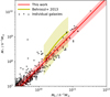 |
Fig. 1. Stellar mass M⋆ as a function of halo mass Mh (SMHM relation) for individual galaxies in the hydro-simulation (black dots), and a power law fit (red) to this distribution. For comparison, a model of the SMHM relation by Behroozi et al. (2013) extrapolated to z = 8.8 is shown in yellow. Shaded areas show the 68% scatter. |
Fitting a power law to the distribution for masses above 109 M⊙, we find that the stellar mass is related to the halo mass roughly as
 (14)
(14)
Behroozi et al. (2013) present a model of the stellar mass–halo mass (SMHM) relation which is consistent with observed stellar mass functions, specific SFRs, and cosmic SFRs from z = 0 − 8. Extrapolating the model to z = 8.8 (in the Mh range that Behroozi et al. (2013) use for z = 8), Fig. 1 shows that our SMHM relation are in rough agreement with their model (see also Somerville & Davé 2015 for a more recent review). In the following figures, most quantities are shown as functions of halo mass, because this is what is predicted from the HMF, but a secondary x axis in the top of the plots display an approximate scale for the corresponding stellar mass, based on the SMHM relation in Eq. (14).
As discussed in Sect. 3.3, a fraction of the stars emit enough ionizing radiation to give rise to Lyα emission; from the H II regions, assuming a Salpeter (1955) IMF, 1.1 × 1042 erg s−1 is produced per SFR of 1 M⊙ yr−1 (Kennicutt 1998), while for a Chabrier (2003) IMF the Lyα luminosity is a factor ∼1.8 times higher, with a modest dependency on stellar mass. In addition to this, accreting gas is shock-heated, subsequently cooling and emitting Lyα, as discussed in Sect. 3.3.2. Figure 2 show the “intrinsically” emitted Lyα – that is, before any RT effects – for the two processes. If Lyα did not scatter, nor were absorbed by dust, this would result in the flux shown with the secondary y.
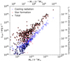 |
Fig. 2. Total, “intrinsically” emitted Lyα |


Figure 3 shows the ratio  in our galaxy sample. Overplotted is the relation theoretically predicted in Sect. 3.3.2, varying all parameters in the discussed ranges (red), and varying all except for the mass loading slope β (blue), which is kept constant at −2/3; this particular slope describes energy-driven winds, which is the way in which we have implemented the winds in our simulations.
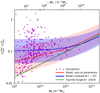 |
Fig. 3. Ratio |

For comparison, the green line shows the relation as calculated by Faucher-Giguere et al. (2010). For large masses, all three models roughly converge. However, for small masses our models predict a larger fraction of cooling radiation, mainly because we explicitly included a model for gas ejection; due to the shallower potential of small galaxies gas is more easily expelled, thus lowering the SFR and hence increasing the ratio.
For masses up to Mh ∼ 1010 h−1 M⊙, star formation in our simulations is rather stochastic so that the ratio fluctuates quite a lot; in some cases, cooling radiation can even dominate the total (albeit small) luminosity.
4.2. UV luminosity function
As discussed in the introduction, the Lyα luminosity is primarily linked to star formation, specifically the massive O and B stars. Since these stars are responsible not only for Lyα but for the bulk of the entire UV spectrum, the Lyα LF and the UV LF are intrinsically connected (see, e.g. Gronke et al. 2015), so comparing the predicted UV LF to observations will support our confidence in the simulations. Because of the small size of our cosmological volume, it cannot be used to determine the HMF. Instead we use the ST HMF (Eq. (1), calibrated to the Bolshoi simulation) to give us the number density of halo masses, and then translate this to an LF by using the relation between halo mass and brightness for our simulated galaxies. That is, with halo number density and masses measured in h3 Mpc−3 and h−1 M⊙, respectively, the LF can be written as
 (15)
(15)
In the Sect. 4.2.1. below, we describe how to obtain the final term in Eq. (15).
4.2.1. Relation between halo mass and UV luminosity
Trac et al. (2015) argue for a triple power law relation between the UV luminosity and the halo masses. Expressed in terms of magnitudes,
![Mathematical equation: $$ \begin{aligned} M_{\rm {UV}} =& -2.5 \left[ \log L_0 + a \log \left( \frac{M_{\rm {h}}}{M_{\mathrm{h} ,a}} \right) \right. \nonumber \\ &+ (b-a)\left. \log \left(1 + \frac{M_{\rm {h}}}{M_{\mathrm{h} ,b}} \right) \right. \\ &+ (c-b)\left. \log \left(1 + \frac{M_{\rm {h}}}{M_{\mathrm{h} ,c}} \right) \right] + 51.6 \nonumber \end{aligned} $$](/articles/aa/full_html/2019/07/aa33645-18/aa33645-18-eq35.gif) (16)
(16)
where L0 is an overall amplitude, Mh, a, Mh, b, and Mh, c are three characteristic mass scales, and a, b, and c are three power law slopes.
To determine the UV magnitudes of the simulated galaxies, each galaxy’s UV spectrum is calculated using the stellar population synthesis code STARBURST99 (Leitherer et al. 1999). Subsequently, for each galaxy 104 sightlines are followed from the locations of star formation in random directions, with the probability of starting a sightline from a given location proportional to the UV luminosity of stars in that region. Integrating dust extinction along the lines of sight, we obtain a distribution of observed UV magnitudes at 1600 Å in different directions.
Figure 4 shows the halo mass–magnitude relation thus obtained, with the reddened values (red points with error bars) showing the median and the 68% scatter. Comparing to the unreddened values (blue points), effects of reddening are seen to only affect the most massive galaxies, with M⋆ ≳ 109 h−1 M⊙.
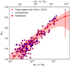 |
Fig. 4. UV magnitude MUV at 1600 Å as a function of halo mass Mh. For each galaxy the “intrinsic” UV magnitude calculated with STARBURST99 (blue dots) and the reddened magnitudes calculated using the median and 68% scatter of the luminosity-weighted extinction along isotropically distributed sightlines from the star (red dots with error bars) are shown. The red line shows the best fit of the analytical relation in Eq. (16), with the red shaded region showing the prediction interval within which 68% measurements would fall. Only the most massive galaxies are seen to have UV escape fraction significantly below unity, with the red points falling below the blue. |
In addition to the simulated MUV magnitudes, the best fit of the functional form in Eq. (16) with 68% PI is shown in red. At low masses, this PI primarily reflects a scatter in the galaxies’ intrinsic luminosities, while at high masses the anisotropic escape of the UV radiation due to dust, as well as the fact that we have so few galaxies more massive than ∼1011 M⊙ comes into play. The overturn of the 16th percentile to lower values of MUV at high Mh is not necessarily unphysical, but is quite uncertain. We note that this anisotropic escape of UV photons is not necessarily correlated with the anisotropic escape of Lyα.
4.2.2. Comparing to observations
The derivative of Eq. (16), needed to evaluate Eq. (15), is
 (17)
(17)
The parameters of the fit to MUV(Mh) (Eq. (16)) can now be plugged into Eq. (17), which in turn enables us to evaluate the UV LF Eq. (15). Due to the small number of galaxies detected at such high redshift, no concensus of a z ∼ 9 LF exists, but Bouwens et al. (2015) report a rather well-constrained UV LF at z ∼ 8, as well as a less well-constrained one around z ∼ 10 which is improved in Oesch et al. (2018). Figure 5 shows our calculated UV LF, together with the those observations. It is reassuring to see that the z = 8.8 LF lies between those of z ∼ 8 and z ∼ 10.
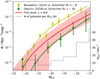 |
Fig. 5. Luminosity function Φ at 1600 Å of the simulated galaxies (red solid). The red shaded region shows the 68% spread in Φ, which at the faint end reflects a scatter in the intrinsic UV luminosity, and at the bright also the anisotropic escape of UV radiation due to dust, as well as small-number statistics. Yellow and green dots with error bars show the observed LFs at z ∼ 8 (Bouwens et al. 2015) and z ∼ 10 (Oesch et al. 2018), respectively, with the associated solid lines showing the best-fitting Schechter (1976)-functions. The number of simulated galaxies used for our fit is shown in solid black, with the corresponding numbers on the right y axis. |
We note, however, that the LF at MUV ≲ −20 is quite uncertain, with the sharp drop of the 16th percentile is caused by the overturn seen in Fig. 4.
4.3. Typical line shapes
The most prominent feature of an LAE is arguably the emission line profile, and much valuable knowledge can be extracted from it. Scattering on neutral hydrogen slowly pushes the photons farther from the line centre, so larger column densities are associated with broader emission lines. The same is true for larger temperatures, as the thermal motion of hotter atoms will engender larger Doppler shifts (e.g. Harrington 1973; Neufeld 1990). The relative height of the red and the blue peaks provides a measure of the global kinematics of the galaxy, since blue (red) photons are suppressed by outflowing (infalling) gas, by being Doppler-shifted into the frame of reference of the gas elements (e.g. Dijkstra et al. 2006). At higher redshifts the blue peak is also influenced by the CGM (e.g. Laursen et al. 2011). The longer the photons travel, the more prone they are to dust absorption, so photons emitted in the dense and dusty star-forming regions, which would have to scatter to the wings of the spectrum, escape less easily than photons emitted in the outskirts of the galaxy (e.g. from cooling radiation). As a result, dust is expected to narrow the spectrum (Laursen et al. 2009b). However, the intertwinement of these effects also makes the interpretation of Lyα observations notoriously difficult, motivating the need for a more profound theoretical understanding.
Figure 6 shows the median spectra for galaxies in different mass ranges.
 |
Fig. 6. Median spectra of galaxies in various halo mass ranges, normalized to the same stellar mass (109.5 h−1 M⊙), and including the impact of the IGM on the line. The shaded areas show the 68% PIs. Although the median flux in the line hardly rises above the continuum, prominent lines are seen for a significant fraction of the galaxies. Also shown (using the right y axis) is the median transmission of the 16 filters (yellow), and the IGM transmission 𝒯(λ) (black), with the shaded regions showing the 68% scatter. |
In the figure, the spectra have been normalized to the same stellar mass, namely M⋆ = 109.5 h−1 M⊙, which is the mass of the most massive mass range. In each mass range ten to tweny galaxies have been used, and for each galaxy, the median and the dispersion of six directions, each with 100 different realizations of the impact of the IGM, has been used. While the typical spectrum of even the most massive galaxies is virtually erased by the IGM, within 1σ many lines do rise above the continuum. Despite the normalization, the lines decrease somewhat in intensity with decreasing stellar mass. While this may in part be attributed to less cooling radiation, the main reason is that more massive galaxies are more likely to ionize larger bubbles around themselves, facilitating the transfer of Lyα.
4.4. Escape fractions
As soon as the first generation of stars end their lives, the ISM is polluted with metals. A fraction of these metals deplete to form dust grains. As galaxies must probably have gone through at least some star formation episodes to make themselves visible, it therefore comes as no surprise that most visible galaxies must also contain some amount of dust. Because of the long path length of Lyα (compared to continuum photons) due to scattering, Lyα is particularly prone to dust absorption4. Observationally, it is difficult to distinguish between photons lost to dust and photons scattered out of the LOS by the IGM, but in the simulations this is possible. However, only the most massive galaxies have been able to generate enough dust to give to a measurable colour excess; thus, averaged over all directions the Lyα escape fraction fesc is close to unity. Nevertheless, the complex density field entails a quite anisotropic escape, where some sightlines are blocked by dense clouds, instead beaming the radiation in other directions. Defining the escape fraction as the ratio of observed Lyα flux to what would be observed if all photons escaped isotropically, fesc will thus exceed unity in some directions. This is seen in Fig. 7, where the large spread between different sightlines is also noticed. It should be noted that that part of the spread in the median of the escape fractions is due to averaging over only six directions.
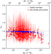 |
Fig. 7. Escape fraction fesc of Lyα as a function of halo mass Mh, defined as the ratio of the number of Lyα photons that make it out through the galaxy to the total number emitted (i.e. if there were no dust and galaxies were isotropic, fesc would be unity in all directions). The red points and the error bars denote the median and the 68% scatter of the six directions along the Cartesian axes, while the blue points show the global average. The extent of the error bars is chiefly dictated by the anisotropy of the ISM, but the scatter in the median values is partly due to only using six directions for the statistics. Only for galaxies above Mh ∼ 1010 h−1 M⊙ does dust play a significant role for the escape fraction. After escaping the galaxy, photons may still be scattered out of the LOS, so the observed fesc would be (much) smaller than these values. To guide the eye, a dashed, grey line is shown at fesc = 1. |
4.5. Optimal aperture
As discussed in Sect. 3.3.3, scattering in the IGM persists out to many virial radii. Photons travelling in the direction towards the observer are lost from the LOS, but do not vanish; instead they become part of the Lyα background. Similarly, photons that initially leave the galaxy in another direction, have a small chance of being scattered towards the observer. This mechanism creates a halo of Lyα light around the galaxy, which has indeed been observed at all redshifts down to z ∼ 0 (Hayes et al. 2013; Leclercq et al. 2017).
The half-light radii of our simulated galaxies increase from a few kpc, to roughly 5 kpc, to ∼10 or even tens of kpc for small, intermediate, and massive halos, respectively. When measuring the total flux received from a galaxy, a larger aperture will always result in more flux, but also in more background noise. The standard aperture for measuring flux has a diameter of 2″, corresponding at z = 8.8 to just under 10 kpc. For the most massive galaxies, which as yet are the only ones we have a chance of detecting, we will hence miss of the order half of flux (see Fig. 8).
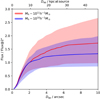 |
Fig. 8. Measured flux as a function of aperture diameter Dap, normalized to the flux measured at Dap = 2″, for Mh ∼ 1011 h−1 M⊙ (red) and Mh ∼ 1010 h−1 M⊙ (blue) galaxies, with the shaded regions giving the 68% PI. For the Mh ∼ 1011 h−1 M⊙ galaxies, the observed flux for Dap = 2″ is ∼50% compared to Dap → ∞, but since a smaller Dap means less noise, slightly better results are achieved for |

In fact, due to the increased noise for large apertures, the “optimal” aperture turns out to be a slightly smaller 1 4, although the difference in the total number of observed galaxies is on the < 10% level when comparing to using a 2″ aperture.
Sadoun & Zheng (2016) similarly discuss the fraction of photons that fall outside an aperture of diameter 2″ for a strong and a weak ionizing background. For the weak UVB, corresponding to early in the EoR, they predict that the flux should be suppressed by a larger factor of approximately ten. However, their LAE model is modeled as a smooth gas distribution, which forces photons to scatter to larger distances than in a clumpy medium before being able to escape.
4.6. Translating flux threshold to minimum observable mass
Figure 9 shows the expected observed flux F measured within a 1 4 circular aperture centred on the brightest pixel for the simulated galaxies as a function of their halo mass. Viewing the galaxies from different directions introduce a large scatter in the observed flux, both due to the anisotropy of the galaxies, and due to the inhomogeneous IGM. The scattered points show the median observed flux (i.e. of the radiation that makes it through both ISM and IGM), while the error bars show the 68% scatter in the flux introduced by the anisotropic ISM alone.
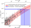 |
Fig. 9. Flux F measured inside a 1 |

Assuming a power law-like relation between F and Mh (which should be suitable at least over a limited mass range), but with a turnover at high masses where dust and possibly a more compact ISM makes Lyα escape harder (see Laursen et al. 2009b), a double power law given by
 (18)
(18)
with  is found, through a non-linear least squares fit using Python’s curve_fit algorithm, as the best fit to the data in the relevant range (the negative exponent in the last term probably makes this functional form impractical at higher masses). The red, shaded region captures the 68% PI from both the anisotropic escape, the inhomogeneous IGM, and the spread in flux from galaxies of similar masses. If instead we fit a single power law, so there is no turn-over at high masses, the resulting value of Mh, min is a bit smaller; we return to discussing the consequences of this and the related confidence of the fit in Sect. 4.7.2.
The 16 detectors of UltraVISTA have a varying threshold for detecting sources at a given significance, and even have variations in different regions of the detectors. For a 5σ detection and an aperture of 1 4, they have an median threshold of mAB, thres = 25.25 ± 0.24, corresponding to a flux threshold of
  , shown in Fig. 9 as the horizontal, blue, dashed line with the shaded region indicating the spread. These values are as measured in a 1
 4 aperture, and do not include an aperture correction, since we measured the flux in our simulated images using this aperture.
The first thing to notice is that indeed some of the simulated galaxies make it above the flux threshold, at least in certain directions – the question is whether such galaxies are sufficiently common that there is a significant probability that UltraVISTA will detect them. Assuming the relation Eq. (18) to hold true, this flux threshold can be translated into a minimum observable halo mass
 (19)
(19)
seen in Fig. 9 as the vertical blue dashed line. This corresponds roughly to a minimum observable stellar mass of  .
.
4.7. Translating minimum observable halo mass to expected number of observed galaxies
Integrating the HMF from a given mass scale M′ to infinity, we can find the total number of haloes that are at least as massive as M′. Figure 10 shows the resulting cumulative halo mass function in the volume surveyed by UltraVISTA.
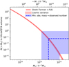 |
Fig. 10. Cumulative halo mass function (solid red), normalized to the approximate volume surveyed by UltraVISTA. The red shaded region represents the 1σ standard deviation on the number counts resulting from cosmic variance. The dashed blue line shows the minimum observable halo mass (Eq. (19)) in the UltraVISTA survey and the corresponding number of observed galaxies. The blue shaded region shows the 68% PI for this. |
4.7.1. Cosmic variance
Density fluctuations in the large-scale structure lead to uncertainties in the number counts, known as cosmic variance. The expected standard deviation due to this effect is shaded red in Fig. 10. This uncertainty is obtained following Trenti & Stiavelli (2008), who estimate the cosmic variance employing a combination of excursion set theory (Bond et al. 1991) and N-body simulations. We have made use of the associated online calculator5, which allows for a Sheth & Tormen (1999) bias instead of a Press & Schechter (1974) bias, as well as changing the value of σ8 to our preferred value of 0.82. All their simulations have {ΩM, ΩΛ}={0.26, 0.74}, rather close to the {0.27, 0.73} of the Bolshoi simulation. Taking into account cosmic variance results in a relative uncertainty on the number of galaxies increasing from 17% at Mh = 1010 h−1 M⊙ to 48% at Mh = 1012 h−1 M⊙.
The vertical blue dashed line shows the minimum observable halo mass Mh, min, discussed in the previous section, and the horizontal line shows the corresponding number of galaxies that will be observed. When the 68% PI of the Mh, min, shown as the blue shaded region, is combined with the cosmic variance, the resulting expectation value of the number of observed galaxies is  .
.
4.7.2. Poisson noise
In addition to cosmic variance, there will be an uncertainty from usual Poisson noise. For large values of N, the Poisson noise converges towards  , but for small values this approximation becomes increasingly inaccurate, as the 68% confidence interval (CI) becomes increasingly asymmetric6.
Since the number of galaxies is an integer, it makes little sense to quote a number such as that found in the previous section; instead it is more illuminating to find the probability of detecting a given integer number. From the standard definition of the Poisson distribution, we can then finally state the disheartening probabilities of observing none, one, or two or more galaxies as
 (20)
(20)
One should perhaps not place too much significance in the exact probabilities. As mentioned in Sect. 4.6, if the flux-mass relation in Fig. 9 is fitted with a single, rather than double, power law, the detection threshold intercepts the fit at slightly lower value of  , implying an expected number of detections of
  , and probabilities
  %. Considering the results from the two fits, we report the result as roughly 90%, 10%, and 1% chance of observing zero, one, or two or more galaxies in the survey, respectively.
4.8. Luminosity function
Following the same approach as in Sect. 4.2, a Lyα LF can be constructed. This is seen in Fig. 11, where we also compare to the models presented in Nilsson et al. (2007) and Matthee et al. (2014); the latter is an upper limit LF allowed by the limits of their survey.
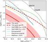 |
Fig. 11. Lyα LF predicted from our simulations (red with shaded area showing the 68% PI), compared to the three models of Nilsson et al. (2007, described in Sect. 1). Also shown, with the red dashed line, is the Lyα LF predicted from our simulations if we did not take into account RT effects. Additionally, the upper limit LF of Matthee et al. (2014) is shown in green. The grey region marks observational upper limits from Willis & Courbin (2005) and Cuby et al. (2007). |
Our LF lies well below all models, but is less steep at the bright end than the closest models.
Figure 11 also shows how the predicted Lyα LF would look if we did not take into account Lyα RT. At the bright end, this differs from the correct LF by almost two orders of magnitude, highlighting the crucial role of a proper RT treatment.
5. Discussion
5.1. Colour selection – different impact of the IGM on narrowband and broadband observations
In Sect. 4.7 we predicted that the probability of detecting just one, or two or more, z = 8.8 galaxies in the NB118 image of the final UltraVISTA survey is of the order of 10% and ≲1%, respectively. But even if a galaxy is brighter than the detection threshold, it still needs to be selected as a candidate z = 8.8 emitter. How to do this is not as simple as identifying a galaxy having emission from a rest frame optical line – where it is essentially a question of having a higher flux density in a NB than in a broad band (BB) – as we will discuss here:
If there were no emission line, a flat spectrum would have mNB − mBB = 0, where in this case mNB is the magnitude in the Lyα NB118 filter, and mBB is the J band magnitude. However, at redshifts that are high enough for the IGM to suppress all flux blueward of the line – both line and continuum – and even a significant part of the red half, NB and BB magnitudes are affected differently. The reason is that the NBs are centred on the line, so that (less than) 50% of the flux is transmitted, whereas in the J band – which transmits in λ ∼ [11 650–13 500] Å – the Lyα break is located quite far to the blue, so that roughly 85% is transmitted. For 50% transmission in the NB, a flat spectrum with no emission line would then have a colour of mNB − mBB = −2.5log(50/85)≃0.6. In reality, because the IGM erases a significant part of the flux – again both line and continuum – redward of the line centre the NB transmission is closer to 25%, in which case the colour of a line-less spectrum lies at ∼1.3. In these calculations, the Lyα line centres have been assumed to coincide with the NB centre.
Figure 12 shows a colour-magnitude diagram of the simulated galaxies.
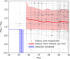 |
Fig. 12. Colour-magnitude diagram of the simulated galaxies. Black dots show individual galaxies, with grey error bars showing the 68% scatter for different sightlines. The red line shows a running median (with shaded 68% PI) of the mNB − mBB colour as a function of NB magnitude for all galaxies when we artificially remove their Lyα emission lines. The selection criteria are shown with blue dashed lines; the magnitude threshold is the same as in Sect. 4.6, while the colour threshold is set to mNB − mBB < +0.85, corresponding roughly to the lower limit of the “no Lyα”. Although no galaxy on average falls inside the selection square, the directional variance results in a probability of a few tens of % of being selected, albeit for the brightest galaxies only. |
The error bars correspond to different sightlines. To calculate a more realistic colour of a line-less spectrum than the qualitative estimate in the preceding paragraph, the colours and magnitudes are also calculated were we artificially remove the Lyα emission from the synthetic spectra before calculating the NB and BB magnitudes. In this case, the scatter is much smaller and is caused mainly by inhomogeneities in the IGM. A running median (with 16th and 84th percentiles) of the galaxies’ colours in this case is shown in the figure in red. The median colour is seen to be rather independent of NB magnitude, with a value around mNB − mBB ≃ 1.25, except for the brightest galaxies where dust begins to play a role; here the reddening causes a slight upturn in the colour index. The lower limit of the 68% PI lies around mNB − mBB ≃ +0.85. Using this value as the colour threshold, together with the magnitude limit of the individual detectors, a “selection square” is defined, shown with blue, dashed lines in Fig. 12 (the blue-shaded region shows the spread in the detector limits).
Considering only the median colours and magnitudes of the galaxies, not even the brightest ones fall inside the selection square. However, taking into account the variability in brightness in different directions, the brightest ones do in fact have a non-zero probability Psel of being selected as LAEs. The brightest galaxy in the sample, which is also the most massive with Mh = 3.4 × 10¹¹ h−1 M⊙, has a 35% chance of being selected, that is, to meet the colour selection criterion and being brighter than the detection limit of the survey. There is no clear trend of Psel with halo mass, but for Mh ≳ 1011 h−1 M⊙, Psel lies between a few % and 35%, while for Mh ≲ 1011 h−1 M⊙, Psel is virtually zero.
5.2. Halo mass function and cosmology
The HMF was, and typically is, calculated considering dark matter only. Although baryons make up only ∼0.16 of the total mass, their ability to cool and condense leads to more concentrated mass profiles, resulting in principle in higher halo masses. Thus, Stanek et al. (2009) and Cui et al. (2012) find an increased number density of cluster scale haloes in simulations including gas cooling and star formation. However, also taking into account the effect of AGN feedback prevents overcooling of the gas, counteracting this concentration. Martizzi et al. (2014) find that, incidentally, the resulting mass function is quite close to the DM-only HMF. We therefore choose to ignore baryonic effects on the HMF.
Of greater concern might be the functional form of the multiplicity function f(σ) (Eq. (4)). Both the PS and the ST HMFs are “universal”, in the sense that their multiplicity functions are independent of power spectrum and expansion history of the Universe. Several successive authors have noted departures from universality (e.g. Tinker et al. 2008; Crocce et al. 2010; Watson et al. 2013). Tinker et al. (2008) let the parameters of f(σ) be a function of redshift, and in the BolshoiP simulation (an “updated” version of the Bolshoi simulation with Ade et al. 2016 cosmology), Klypin et al. (2016) showed that this HMF fits their halo abundances well, albeit only in the range 0 < z < 2.5.
Behroozi et al. (2013) extended the Tinker et al. (2008) HMF to z = 8, although only for masses up to Mh ∼ 1011.5 h−1 M⊙, which is lower than the upper limit for the minimum detectable mass in UltraVISTA. However, Rodríguez-Puebla et al. (2016) provide a fitting formula for a HMF that gives good fits to the BolshoiP simulation at higher masses. Extending that fit to z = 8.8 increases the number density of haloes with masses around the minimum detectable halo mass four-fold from the  found in Sect. 4.7.1 to
  or, in terms of probabilities of detecting an integer number of galaxies,
  %. This would seem to imply that, although a non-detection is still the most likely outcome, the prospects of finding a few are less pessimistic. However, as mentioned in Sect. 3.2, since in the Ade et al. (2016) cosmology the Universe reionizes later, this would counteract detectability.
5.3. Field galaxies vs. cluster galaxies
The fact that the galaxies are taken from a proto-cluster region might be a concern, since they could evolve differently from a “typical” galaxy. However, although cluster galaxies form earlier, and peak earlier in star formation, than field galaxies, the two have comparable specific SFRs (Muldrew et al. 2017). Since our model assigns a brightness to a galaxy based on its mass, but the mass distribution itself is taken from the HMF, which is unrelated to the simulated galaxies, we do not consider this to be an issue.
5.4. Ionization state of the IGM
The largest uncertainty in our forecast is arguably the ionization state of the IGM. Although the LyC RT is treated accurately, it hinges on the assumed evolution of the UVB field. The global neutral fraction in our hydro-simulation is xH I ≃ 0.13, but in the IGM the fraction is much lower, of the order 10−4–10−3. This is still enough to erase the blue part of the Lyα line, and the CGM and residual neutral clumps cause the damping wing to erase a large part of the red wing as well.
Even if we have overestimated the impact of the CGM/IGM, it is hard to imagine that even a small fraction of the blue wing escapes; although some galaxies are surrounded by highly ionized bubbles, galaxy and quasar spectra show complete Gunn-Peterson troughs (e.g. Fan et al. 2005; see however Hu et al. 2016 and Matthee et al. 2018 for a counterexample at z = 6.6) If we redo our analysis by simply removing the blue half of the spectrum – thus neglecting the effect of the damping wing – the expected number of detected LAEs increases to  . Only if we completely neglect the IGM do we predict a large success rate, with
  .
.
We have not considered alternative SEDs for our LyC RT. Harder UV fields, for example preticipated by binary stars, lead to larger LyC escape fractions (Stanway et al. 2016; Ma et al. 2016; Rosdahl et al. 2018), implying an earlier EoR. The increased UV flux also leads to lower H I column densities in the ISM, facilitating the escape of Lyα from the ISM. At these high redshifts where there is not much dust, Lyα escape fraction are close to unity anyway, but a lower NH I means that the Lyα photons escape closer to the line centre. However, this actually impedes their escape through the IGM; when the photons are far from the line centre, at least the part that are in the red wing may have a chance of escaping (as they are only redshifted further from resonance when travelling through the expanding Universe); but when they are close to the line centre, the large damping wing of the IGM absorption makes the photon scatter until they are farther from the galaxy. The combined effect of the earlier EoR and the easier escape is difficult to predict without new simulations. The effect could also be counteracted to some extent by the fact that the increased feedback might have a tendency to reduce star formation.
5.5. Starburst-driven outflows
When massive stars explode as supernovae, they heat up the ISM, causing it to expand and form bubbles. If the SN explosion rate is sufficiently high, the SN remnants overlap before they can cool radiatively, in which case these bubbles – assisted by super-Eddington photon pressure – may extend beyond galactic scales, manifesting themselves as outflowing superwinds (see e.g. Powell et al. 2011, and references therein).
Such winds have been observed at lower redshifts, mainly through blueshifted absorption lines (e.g. Kunth et al. 1998; Pettini et al. 2001; Shapley et al. 2003), and are usually thought to be the explanation for the often-observed asymmetric Lyα line profiles (e.g. Verhamme et al. 2006; Tapken et al. 2007; Yamada et al. 2012; Erb et al. 2014), where the red peak is enhanced with respect to the blue. One of the largest uncertainties in hydro-simulations in general is arguably how the feedback from stellar energy output affects the surrounding gas. Although many cosmological simulations have employed various implementations of feedback that are able to generate outflows, when it comes to Lyα RT in general the predicted line profiles tend to be rather symmetric (e.g. Tasitsiomi 2006; Gronke & Bird 2017) or even have an increased blue peak (e.g. Laursen & Sommer-Larsen 2007; Barnes et al. 2011; Yajima et al. 2012; Smith et al. 2015). That is, despite gas being ejected from the galaxies, infalling gas accreting onto the galaxies dominate the kinematics, leading to the opposite effect. Only in simulations of isolated disc galaxies has a prominent red peak been successfully reproduced, and only when observed face-on where the wind is strongest (Verhamme et al. 2012).
One may surmise that the asymmetric profile be created on scales much smaller than what is usually resolved, for example by stellar winds inside the H II regions where most of the Lyα is produced, so that in effect photons in a simulation like our have a larger probability of being “injected” redward of the line centre. However, even simulations of Lyα escape from molecular clouds with sub-parsec resolution seem to produce quite symmetric line profiles (Kimm et al. 2019). Moreover, even if they did begin from the sources shifted from the centre, it is not clear that it would result in global asymmetric profiles, since subsequent scattering in a static medium has a tendency to “pull” photons back toward the line centre (Osterbrock 1962).
Observations based primarily on O VI absorption lines indicate that the CGM around star-forming galaxies at z ∼ 0 contains considerable amounts of oxygen (e.g. Tumlinson et al. 2011; Prochaska et al. 2011). Also lower-ionization species such as Si II, Si III, and N II are detected (e.g. Prochaska et al. 2017, and references therein). Based on observations of potential O VII absorption in the hot CGM of the Milky Way, Gupta et al. (2012) infer the presence of large amounts of oxygen in the CGM as well (see however Wang & Yao 2012).
Computer simulations indicate that models based on inefficient stellar feedback (“low”-feedback models) cannot reproduce the level of O VI column densities observed in the CGM to impact parameters of 150–200 kpc (e.g. Stinson et al. 2012, 2013; Hummels et al. 2013). The simulations presented in this work were stopped at z = 8.8, but in another project (Sommer-Larsen & Laursen, in prep.), the same code was used to simulate the formation and evolution of eight field disc galaxies to z = 0 in a cosmological context using the zoom-in technique. At z = 0, the galaxy luminosities, stellar masses, and specific SFRs span the ranges L ∼ 0.2 − 0.6 L⋆, M⋆ ∼ 3 − 6 × 10¹⁰ M⊙, and sSFR ∼ 0.04 − 0.1 Gyr−1, respectively.
For each of the eight galaxies, 6800 sightlines are shot through the galaxy in random directions and with impact parameters b spanning the range b = 2 − 500 kpc. Along each LOS the total O VI column density NO VI is determined. Averaging over the eight galaxies, Fig. 13 shows the median NO VI as a function of impact parameter b, compared to the observational data from Tumlinson et al. (2011) for “star-forming” galaxies (sSFR ≳ 0.01 Gyr−1) of luminosities in the range L ∼ 0.1 − 1 L⋆. As can be seen from the figure, the match between simulations and observations is quite acceptable, indicating that the simulations capture at least these outflow properties correctly – see also Sommer-Larsen & Fynbo (2017) for the case of the high-impact parameter and high-metallicity DLA towards Q0918+1636, at z = 2.58; this system is very well reproduced by simulations based on a code similar to the one utilized in this work, and it is shown that by far the majority of the α-element absorption seen in this system at galacto-centric distances ≳20 − 30 kpc is caused by metals that have been produced in the inner part of the galaxy, and subsequently transported outwards by galactic winds.
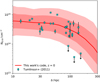 |
Fig. 13. Median O VI column density NO VI (red) as a function of impact parameter b, averaged over 6800 sightlines through eight z = 0 disc galaxies simulated using the same code as the one utilized in this work. Shaded regions indicate the 1σ and 2σ deviations from the median, respectively. The observations of “star-forming” galaxies by Tumlinson et al. (2011) are shown by cyan squares. |
6. Summary and conclusions
We have numerically explored the prospects of detecting Lyα-emitting galaxies on the verge of the Epoch of Reionization. To ensure both good number statistics and high resolution, we employed a combination of a semi-analytical halo mass funtion matched to a large-scale N-body simulations and zoom-in simulations of hydrodynamical, cosmological simulations. This was combined with accurate RT schemes of both ionizing UV and Lyα.
Physical uncertainties such as variance in the escape of Lyα in different directions – both out through the ISM of the galaxies and further through the IGM – galaxy-to-galaxy variation, and statistical number variance, as well as observational uncertainties such as differing filter shapes and varying detector exposure, were taken into account. In general, such uncertainties are asymmetrical, and a numerical scheme for adding asymmetrical errors is described (in Appendix B) and made public.
With these simulations we have been able to predict a number of physical characteristics of galaxies at redshift z = 8.8. Our stellar mass–halo mass relation is consistent with the observationally based model by Behroozi et al. (2013), extrapolated to z = 8.8. At the investigated redshift the Lyα LF is largely unconstrained, but the predicted UV LF is shown to be consistent with observations.
Our main findings – which apply to z = 8.8 – are:
-
Scattering in the CGM prevents Lyα from escaping a galaxy until large distances from its emission site. This results in of the order of half of the flux falling outside standard apertures. However, since larger apertures also implies more noise, it does not help to enlarge it, and in fact we find that, for the UltraVISTA survey, an aperture of 1
 4 results in a slightly larger probability of detecting a galaxy.
 -
Scattering in the IGM erases completely the blue part of the spectrum, and a large fraction (∼25%) of the red half. This means that, on average, the Lyα line is suppressed to continuum level.
-
The escape of Lyα is, however, very dependent on the direction from which a galaxy is observed. Both the anisotropy of the ISM, and inhomogeneities in the transmittance of the IGM, results in the spectra exhibiting prominent peaks in a significant fraction of directions, enabling us to see them in some cases (see Fig. 6).
-
Accurate treatment of the Lyα RT and the halo number statistics enables us to predict the expected number of LAEs in the UltraVISTA survey; the probabilities of detecting none, one, or two or more LAEs are roughly 90%, 10%, and 1%, respectively (see Eq. (20)).
-
Since the Lyα break lies far to the blue in the J broadband filter, and since the damping wing of the IGM absorption extends far into the red wing of Lyα, the IGM suppresses a much smaller fraction in BB than in the NB. Thus, a colour selection criterion of mNB − mBB ≲ 0 may miss many possible LAEs. Simulating the colours of our galaxies without the Lyα emission lines, we show that the lower 1σ limit lies approximately at mNB − mBB = +0.85, which we argue is a better criterion.
-
Using that criterion, we find that even if a galaxy is detectable in the NB, its has only ≲35% chance of being selected as an LAE.
-
We investigated factors that might lead to a larger probability of success. All things being equal, using a Planck cosmology rather than a WMAP7 increases the predicted number of detections from ∼0.06 to ∼0.26, but the associated earlier onset of the EoR might counteract this increased probability. Assuming an unrealistically less aggressive IGM (simply removing the blue wing of the Lyα line) further increase the expected number to ∼0.5, while neglecting the IGM altogether would result in approximately two detections.
On the whole, while the UltraVISTA (broadband) survey has already resulted more than 100 papers directly using the data7 and many more papers using the data via the photometric, photo-z and stellar mass catalogues (Ilbert et al. 2013; Muzzin et al. 2013; Laigle et al. 2016), the hunt for LAEs seems unprofitable. According to our simulations, increasing the probable number of detections to one would require roughly another 1000 h of observations with UltraVISTA. However, as our simulations show that galaxies that are bright enough to be detected with UltraVISTA do indeed exist (Fig. 9), and as the analysis is still in progress, we are still hopeful8,9.
We note that other functional forms of the filter are possible, for example a Gaussian filter for which  , where the relation between mass and radius is Mh = (2π)3/2R3ρM.
See www.vista.ac.uk
With approximately half a detector size between each detector, and an equivalent shift between each of three pointings, each of the four stripes is characterized by 13 different limiting magnitudes (see Fig. 2 of Milvang-Jensen et al. 2013).
We note that, theoretically, it is possible to have the reverse effect, meaning to have a dusty, multi-phase ISM that preferentially lets Lyα escape (Neufeld 1991; Hansen & Peng 2006). However, as shown by Laursen et al. (2013) and Duval et al. (2014) this requires physically unrealistic scenarios; in particular an almost vanishing velocity field together with (super-)solar metallicities and very high density contrasts between the phases.
For instance, the Poisson uncertainty on the numbers 100 and 10, is not ±10 and ±3.16 as one might naively expect, but  and
and  , respectively (Gehrels 1986).
SHARCNET: www.sharcnet.ca.
Acknowledgments
We are most grateful to the anonymous referee for many excellent suggestions and corrections. The Dark Cosmology Centre was funded by the Danish National Research Foundation (DNRF). The Cosmic Dawn Center is funded by DNRF. PL, BM-J, and JPUF acknowledge support from the ERC-StG grant EGGS-278202. Galaxy simulations were performed on the facilities provided by High Performance Computing Centre at the University of Copenhagen. Stellar ionization calculations were performed on the kraken cluster of the Shared Hierarchical Academic Research Computing Network. In the process of writing our HMF calculator, comparisons with results from the online HMF calculator HMFCALC (Murray et al. 2013) have been extremely helpful. As we submitted this article, JSL tragically passed away after a few weeks’ illness. He is deeply missed, both as a superb colleague and as a good friend.
References
- Ade, P. A. R., Aghanim, N., Arnaud, M., et al. 2016, A&A, 594, A13 [NASA ADS] [CrossRef] [EDP Sciences] [Google Scholar]
- Arnaboldi, M., Gadotti, D., Hilker, M., et al. 2017, The Messenger, 168, 15 [NASA ADS] [Google Scholar]
- Barai, P., Monaco, P., Murante, G., Ragagnin, A., & Viel, M. 2015, MNRAS, 447, 266 [NASA ADS] [CrossRef] [Google Scholar]
- Barkana, R., & Loeb, A. 2001, Phys. Rep., 349, 125 [NASA ADS] [CrossRef] [Google Scholar]
- Barlow, R. 2003, ArXiv e-prints [arXiv:physics/0306138] [Google Scholar]
- Barnes, L. A., Haehnelt, M. G., Tescari, E., & Viel, M. 2011, MNRAS, 416, 1723 [NASA ADS] [CrossRef] [Google Scholar]
- Behroozi, P. S., Wechsler, R. H., & Conroy, C. 2013, ApJ, 770, 57 [NASA ADS] [CrossRef] [Google Scholar]
- Bennett, C. L., Larson, D., Weiland, J. L., et al. 2013, ApJS, 208, 20 [Google Scholar]
- Binney, J., & Tremaine, S. 2008, Galactic Dynamics, 2nd edn., (Princeton, USA: Princeton University Press), 1 [Google Scholar]
- Bond, J. R., Cole, S., Efstathiou, G., & Kaiser, N. 1991, ApJ, 379, 440 [NASA ADS] [CrossRef] [Google Scholar]
- Bouwens, R. J., Illingworth, G. D., Oesch, P. A., et al. 2015, ApJ, 803, 34 [NASA ADS] [CrossRef] [Google Scholar]
- Bowman, J. D., Rogers, A. E., Monsalve, R. A., Mozdzen, T. J., & Mahesh, N. 2018, Nature, 555, 67 [NASA ADS] [CrossRef] [Google Scholar]
- Callaway, J., Unnikrishnan, K., & Oza, D. H. 1987, Phys. Rev. A, 36, 2576 [NASA ADS] [CrossRef] [Google Scholar]
- Cantalupo, S., Porciani, C., & Lilly, S. J. 2008, ApJ, 672, 48 [Google Scholar]
- Carroll, S. M., Press, W. H., & Turner, E. L. 1992, ARA&A, 30, 499 [NASA ADS] [CrossRef] [Google Scholar]
- Chabrier, G. 2003, Publ. Astron. Soc. Pac., 115, 763 [CrossRef] [Google Scholar]
- Cole, S., Lacey, C. G., Baugh, C. M., & Frenk, C. S. 2000, MNRAS, 319, 168 [NASA ADS] [CrossRef] [Google Scholar]
- Crocce, M., Fosalba, P., Castander, F. J., & Gaztañaga, E. 2010, MNRAS, 403, 1353 [Google Scholar]
- Cuby, J.-G., Hibon, P., Lidman, C., et al. 2007, A&A, 461, 911 [NASA ADS] [CrossRef] [EDP Sciences] [Google Scholar]
- Cui, W., Borgani, S., Dolag, K., Murante, G., & Tornatore, L. 2012, MNRAS, 423, 2279 [NASA ADS] [CrossRef] [Google Scholar]
- Dijkstra, M. 2014, Publ. Astron. Soc. Aust., 31, e040 [NASA ADS] [CrossRef] [Google Scholar]
- Dijkstra, M., & Loeb, A. 2009, MNRAS, 400, 1109 [NASA ADS] [CrossRef] [Google Scholar]
- Dijkstra, M., & Wyithe, J. S. B. 2010, MNRAS, 408, 352 [NASA ADS] [CrossRef] [Google Scholar]
- Dijkstra, M., Haiman, Z., & Spaans, M. 2006, ApJ, 649, 14 [NASA ADS] [CrossRef] [Google Scholar]
- Dijkstra, M., Mesinger, A., & Wyithe, J. S. B. 2011, MNRAS, 414, 2139 [NASA ADS] [CrossRef] [Google Scholar]
- Duval, F., Schaerer, D., Östlin, G., & Laursen, P. 2014, A&A, 562, A52 [NASA ADS] [CrossRef] [EDP Sciences] [Google Scholar]
- Erb, D. K., Steidel, C. C., Trainor, R. F., et al. 2014, ApJ, 795, 33 [NASA ADS] [CrossRef] [Google Scholar]
- Faisst, A. L., Capak, P., Carollo, C. M., Scarlata, C., & Scoville, N. 2014, ApJ, 788, 87 [NASA ADS] [CrossRef] [Google Scholar]
- Fan, X., Strauss, M. A., Becker, R. H., et al. 2005, AJ, 132, 117 [Google Scholar]
- Fardal, M. A., Katz, N., Gardner, J. P., et al. 2001, ApJ, 562, 605 [NASA ADS] [CrossRef] [Google Scholar]
- Faucher-Giguere, C.-A., Keres, D., Dijkstra, M., Hernquist, L., & Zaldarriaga, M. 2010, ApJ, 725, 633 [NASA ADS] [CrossRef] [Google Scholar]
- Finkelstein, S. L., Papovich, C., Dickinson, M., et al. 2013, Nature, 502, 524 [NASA ADS] [CrossRef] [Google Scholar]
- Furlanetto, S. R., Zaldarriaga, M., & Hernquist, L. 2006, MNRAS, 365, 1012 [NASA ADS] [CrossRef] [Google Scholar]
- Gehrels, N. 1986, ApJ, 303, 336 [NASA ADS] [CrossRef] [Google Scholar]
- Goerdt, T., & Ceverino, D. 2015, MNRAS, 450, 3359 [NASA ADS] [CrossRef] [Google Scholar]
- Goerdt, T., Dekel, A., Sternberg, A., et al. 2010, MNRAS, 407, 613 [Google Scholar]
- Governato, F., Babul, A., Quinn, T., et al. 1999, MNRAS, 307, 949 [NASA ADS] [CrossRef] [Google Scholar]
- Gronke, M., & Bird, S. 2017, ApJ, 835, 1 [NASA ADS] [CrossRef] [Google Scholar]
- Gronke, M., & Dijkstra, M. 2014, MNRAS, 444, 1095 [NASA ADS] [CrossRef] [Google Scholar]
- Gronke, M., Dijkstra, M., Trenti, M., & Wyithe, S. 2015, MNRAS, 449, 1284 [NASA ADS] [CrossRef] [Google Scholar]
- Gupta, A., Mathur, S., Krongold, Y., Nicastro, F., & Galeazzi, M. 2012, ApJ, 756, 4 [NASA ADS] [CrossRef] [Google Scholar]
- Haardt, F., & Madau, P. 1996, ApJ, 461, 20 [NASA ADS] [CrossRef] [Google Scholar]
- Haardt, F., & Madau, P. 2012, ApJ, 746, 125 [NASA ADS] [CrossRef] [Google Scholar]
- Hansen, M., & Oh, P. S. 2006, MNRAS, 367, 979 [NASA ADS] [CrossRef] [Google Scholar]
- Harrington, J. P. 1973, MNRAS, 162, 43 [NASA ADS] [Google Scholar]
- Hashimoto, T., Laporte, N., Mawatari, K., et al. 2018, Nature, 557, 392 [NASA ADS] [CrossRef] [Google Scholar]
- Hayes, M., Östlin, G., Schaerer, D., et al. 2013, ApJ, 765, L27 [NASA ADS] [CrossRef] [Google Scholar]
- Heckman, T. M., Alexandroff, R. M., Borthakur, S., Overzier, R., & Leitherer, C. 2015, ApJ, 809, 147 [NASA ADS] [CrossRef] [Google Scholar]
- Hernquist, L., & Katz, N. 1989, ApJS, 70, 419 [NASA ADS] [CrossRef] [Google Scholar]
- Hopkins, P. F., Quataert, E., & Murray, N. 2012, MNRAS, 421, 3522 [Google Scholar]
- Hu, E. M., Cowie, L. L., Songaila, A., et al. 2016, ApJ, 825, L7 [NASA ADS] [CrossRef] [Google Scholar]
- Hui, L., & Gnedin, N. Y. 1997, MNRAS, 292, 27 [Google Scholar]
- Hummels, C. B., Bryan, G. L., Smith, B. D., & Turk, M. J. 2013, MNRAS, 430, 1548 [NASA ADS] [CrossRef] [Google Scholar]
- Ilbert, O., McCracken, H. J., Fevre, O. L., et al. 2013, A&A, 556, A55 [NASA ADS] [CrossRef] [EDP Sciences] [Google Scholar]
- Iliev, I. T., Shapiro, P. R., McDonald, P., Mellema, G., & Pen, U.-L. 2008, MNRAS, 391, 63 [NASA ADS] [CrossRef] [Google Scholar]
- Iye, M., Ota, K., Kashikawa, N., et al. 2006, Nature, 443, 186 [NASA ADS] [CrossRef] [PubMed] [Google Scholar]
- Jarosik, N., Bennett, C. L., Dunkley, J., et al. 2011, ApJS, 192, 14 [NASA ADS] [CrossRef] [Google Scholar]
- Jensen, H., Laursen, P., Mellema, G., et al. 2013, MNRAS, 428, 1366 [NASA ADS] [CrossRef] [Google Scholar]
- Kennicutt, R. C. 1998, ARAA, 36, 189 [NASA ADS] [CrossRef] [Google Scholar]
- Kimm, T., Blaizot, J., Garel, T., et al. 2019, MNRAS, 486, 2215 [NASA ADS] [CrossRef] [Google Scholar]
- Klypin, A. A., Trujillo-Gomez, S., & Primack, J. 2011, ApJ, 740, 102 [Google Scholar]
- Klypin, A., Yepes, G., Gottlöber, S., Prada, F., & Heß, S. 2016, MNRAS, 457, 4340 [NASA ADS] [CrossRef] [Google Scholar]
- Kollmeier, J. A., Zheng, Z., Dav, R., et al. 2010, ApJ, 708, 1048 [NASA ADS] [CrossRef] [Google Scholar]
- Kunth, D., Mas-Hesse, J. M., Terlevich, E., et al. 1998, A&A, 334, 11 [NASA ADS] [Google Scholar]
- Lahav, O., Lilje, P. B., Primack, J. R., & Rees, M. J. 1991, MNRAS, 251, 128 [NASA ADS] [CrossRef] [Google Scholar]
- Laigle, C., McCracken, H. J., Ilbert, O., et al. 2016, ApJS, 224, 1 [NASA ADS] [CrossRef] [Google Scholar]
- Laursen, P. 2010, ArXiv e-prints [arXiv:1012.2886] [Google Scholar]
- Laursen, P., & Sommer-Larsen, J. 2007, ApJ, 657, L69 [NASA ADS] [CrossRef] [Google Scholar]
- Laursen, P., Razoumov, A. O., & Sommer-Larsen, J. 2009a, ApJ, 696, 853 [Google Scholar]
- Laursen, P., Sommer-Larsen, J., & Andersen, A. C. 2009b, ApJ, 704, 1640 [NASA ADS] [CrossRef] [Google Scholar]
- Laursen, P., Sommer-Larsen, J., & Razoumov, A. O. 2011, ApJ, 728, 52 [NASA ADS] [CrossRef] [Google Scholar]
- Laursen, P., Duval, F., & Östlin, G. 2013, ApJ, 766, 124 [NASA ADS] [CrossRef] [Google Scholar]
- Le Delliou, M., Lacey, C. G., Baugh, C. M., & Morris, S. L. 2006, MNRAS, 365, 712 [NASA ADS] [CrossRef] [Google Scholar]
- Leclercq, F., Bacon, R., Wisotzki, L., et al. 2017, A&A, 608, A8 [NASA ADS] [CrossRef] [EDP Sciences] [Google Scholar]
- Leitherer, C., Schaerer, D., Goldader, J. D., et al. 1999, ApJS, 123, 3 [NASA ADS] [CrossRef] [Google Scholar]
- Ma, X., Hopkins, P. F., Kasen, D., et al. 2016, MNRAS, 459, 3614 [NASA ADS] [CrossRef] [Google Scholar]
- Martin, C. L. 2005, ApJ, 621, 227 [Google Scholar]
- Martin, P. G. 1988, ApJS, 66, 125 [NASA ADS] [CrossRef] [Google Scholar]
- Martizzi, D., Mohammed, I., Teyssier, R., & Moore, B. 2014, MNRAS, 440, 2290 [NASA ADS] [CrossRef] [Google Scholar]
- Matthee, J. J., Sobral, D., Swinbank, A. M., et al. 2014, MNRAS, 440, 2375 [NASA ADS] [CrossRef] [Google Scholar]
- Matthee, J., Sobral, D., Gronke, M., et al. 2018, A&A, 619, A1 [NASA ADS] [CrossRef] [EDP Sciences] [Google Scholar]
- McCracken, H. J., Milvang-Jensen, B., Dunlop, J., et al. 2012, A&A, 544, A156 [NASA ADS] [CrossRef] [EDP Sciences] [Google Scholar]
- McQuinn, M., Hernquist, L., Zaldarriaga, M., & Dutta, S. 2007, MNRAS, 381, 75 [NASA ADS] [CrossRef] [Google Scholar]
- Milvang-Jensen, B., Freudling, W., Zabl, J., et al. 2013, A&A, 560, A94 [NASA ADS] [CrossRef] [EDP Sciences] [Google Scholar]
- Muldrew, S. I., Hatch, N. A., & Cooke, E. A. 2017, MNRAS, 14, 1 [Google Scholar]
- Muratov, A. L., Kereš, D., Faucher-Giguère, C. A., et al. 2015, MNRAS, 454, 2691 [NASA ADS] [CrossRef] [Google Scholar]
- Murray, S., Power, C., & Robotham, A. 2013, Astron. Comput., 3–4, 23 [CrossRef] [Google Scholar]
- Muzzin, A., Marchesini, D., Stefanon, M., et al. 2013, ApJS, 206, 8 [Google Scholar]
- Navarro, J. F., & White, S. D. M. 1994, MNRAS, 267, 401 [NASA ADS] [CrossRef] [Google Scholar]
- Navarro, J. F., Frenk, C. S., & White, S. D. M. 1996, ApJ, 462, 563 [NASA ADS] [CrossRef] [Google Scholar]
- Neufeld, D. A. 1990, ApJ, 350, 216 [NASA ADS] [CrossRef] [Google Scholar]
- Neufeld, D. A. 1991, ApJ, 370, L85 [NASA ADS] [CrossRef] [Google Scholar]
- Nilsson, K. K., Orsi, A., Lacey, C. G., Baugh, C. M., & Thommes, E. 2007, A&A, 474, 385 [NASA ADS] [CrossRef] [EDP Sciences] [Google Scholar]
- Oesch, P. A., Brammer, G., van Dokkum, P. G., et al. 2016, ApJ, 819, 129 [NASA ADS] [CrossRef] [Google Scholar]
- Oesch, P. A., Bouwens, R. J., Illingworth, G. D., Labbé, I., & Stefanon, M. 2018, ApJ, 855, 105 [NASA ADS] [CrossRef] [Google Scholar]
- Oñorbe, J., Garrison-Kimmel, S., Maller, A. H., et al. 2013, MNRAS, 437, 1894 [Google Scholar]
- Osterbrock, D. E. 1962, ApJ, 135, 195 [NASA ADS] [CrossRef] [Google Scholar]
- Partridge, R. B., & Peebles, P. J. E. 1967, ApJ, 147, 868 [NASA ADS] [CrossRef] [Google Scholar]
- Peeples, M. S., & Shankar, F. 2011, MNRAS, 417, 2962 [NASA ADS] [CrossRef] [Google Scholar]
- Peeples, M. S., Corlies, L., Tumlinson, J., et al. 2019, ApJ, 873, 2 [NASA ADS] [CrossRef] [Google Scholar]
- Pengelly, R. M., & Seaton, M. J. 1964, MNRAS, 127, 145 [NASA ADS] [CrossRef] [Google Scholar]
- Pettini, M., Shapley, A. E., Steidel, C. C., et al. 2001, ApJ, 554, 981 [NASA ADS] [CrossRef] [Google Scholar]
- Powell, L. C., Slyz, A., & Devriendt, J. 2011, MNRAS, 414, 3671 [NASA ADS] [CrossRef] [Google Scholar]
- Prescott, M. K. M., Momcheva, I., Brammer, G. B., Fynbo, J. P. U., & Møller, P. 2015, ApJ, 802, 32 [NASA ADS] [CrossRef] [Google Scholar]
- Press, W. H., & Schechter, P. 1974, ApJ, 187, 425 [NASA ADS] [CrossRef] [Google Scholar]
- Prochaska, J. X., Weiner, B., Chen, H. W., Mulchaey, J., & Cooksey, K. 2011, ApJ, 740, 1 [NASA ADS] [CrossRef] [Google Scholar]
- Prochaska, J. X., Werk, J. K., Worseck, G., et al. 2017, ApJ, 837, 169 [NASA ADS] [CrossRef] [Google Scholar]
- Rahmati, A., Pawlik, A. H., Raičevic, M., & Schaye, J. 2013, MNRAS, 430, 2427 [NASA ADS] [CrossRef] [Google Scholar]
- Raiter, A., Schaerer, D., & Fosbury, R. A. E. 2010, A&A, 523, A64 [NASA ADS] [CrossRef] [EDP Sciences] [Google Scholar]
- Razoumov, A. O., & Sommer-Larsen, J. 2006, ApJ, 651, L89 [NASA ADS] [CrossRef] [Google Scholar]
- Razoumov, A. O., & Sommer-Larsen, J. 2007, ApJ, 668, 674 [NASA ADS] [CrossRef] [Google Scholar]
- Rodríguez-Puebla, A., Behroozi, P., Primack, J., et al. 2016, MNRAS, 462, 893 [NASA ADS] [CrossRef] [Google Scholar]
- Romeo, A. D., Sommer-Larsen, J., Portinari, L., & Antonuccio-Delogu, V. 2006, MNRAS, 371, 548 [NASA ADS] [CrossRef] [Google Scholar]
- Rosdahl, J., Katz, H., Blaizot, J., et al. 2018, MNRAS, 479, 994 [NASA ADS] [Google Scholar]
- Sadoun, R., & Zheng, Z. 2016, Miralda-Escudé, J., 7, 1 [Google Scholar]
- Salpeter, E. E. 1955, ApJ, 121, 161 [Google Scholar]
- Schechter, P. 1976, ApJ, 203, 297 [Google Scholar]
- Schroetter, I., Bouché, N., Péroux, C., et al. 2015, ApJ, 804, 1 [NASA ADS] [CrossRef] [Google Scholar]
- Scoville, N., Aussel, H., Brusa, M., et al. 2007, ApJS, 172, 1 [NASA ADS] [CrossRef] [Google Scholar]
- Shapley, A. E., Steidel, C. C., Pettini, M., & Adelberger, K. L. 2003, ApJ, 588, 65 [NASA ADS] [CrossRef] [Google Scholar]
- Sheth, R. K., & Tormen, G. 1999, MNRAS, 308, 119 [NASA ADS] [CrossRef] [Google Scholar]
- Sheth, R. K., & Tormen, G. 2002, MNRAS, 329, 61 [NASA ADS] [CrossRef] [Google Scholar]
- Sheth, R. K., Mo, H. J., & Tormen, G. 2001, MNRAS, 323, 1 [NASA ADS] [CrossRef] [Google Scholar]
- Shibuya, T., Kashikawa, N., Ota, K., et al. 2012, ApJ, 752, 114 [Google Scholar]
- Smith, A., Safranek-Shrader, C., Bromm, V., & Milosavljevic, M. 2015, MNRAS, 449, 4336 [NASA ADS] [CrossRef] [Google Scholar]
- Sobral, D., Best, P. N., Geach, J. E., et al. 2009, MNRAS Letters, 398, 68 [Google Scholar]
- Somerville, R. S., & Davé, R. 2015, ARA&A, 53, 51 [NASA ADS] [CrossRef] [EDP Sciences] [Google Scholar]
- Sommer-Larsen, J., Romeo, A. D., & Portinari, L. 2005, MNRAS, 357, 478 [NASA ADS] [CrossRef] [Google Scholar]
- Sommer-Larsen, J., & Fynbo, J. P. U. 2017, MNRAS, 464, 2441 [NASA ADS] [CrossRef] [Google Scholar]
- Stanek, R., Rudd, D., & Evrard, A. E. 2009, MNRAS, 394, L11 [NASA ADS] [CrossRef] [Google Scholar]
- Stanway, E. R., Eldridge, J. J., & Becker, G. D. 2016, MNRAS, 456, 485 [NASA ADS] [CrossRef] [Google Scholar]
- Stinson, G. S., Brook, C., Prochaska, J. X., et al. 2012, MNRAS, 425, 1270 [NASA ADS] [CrossRef] [Google Scholar]
- Stinson, G. S., Brook, C., Macciò, A. V., et al. 2013, MNRAS, 428, 129 [NASA ADS] [CrossRef] [Google Scholar]
- Stringer, M. J., Bower, R. G., Cole, S., Frenk, C. S., & Theuns, T. 2012, MNRAS, 423, 1596 [NASA ADS] [CrossRef] [Google Scholar]
- Sutherland, W., Emerson, J., Dalton, G., et al. 2014, A&A, 575, A25 [Google Scholar]
- Tapken, C., Appenzeller, I., Noll, S., et al. 2007, A&A, 72, 63 [NASA ADS] [CrossRef] [EDP Sciences] [Google Scholar]
- Tasitsiomi, A. 2006, ApJ, 645, 792 [NASA ADS] [CrossRef] [Google Scholar]
- Thiele, T. N. 1889, Forelæsninger over almindelig Iagttagelseslære: Sandsynlighedsregning og mindste Kvadraters Methode, ed. C. A. Reitzel [Google Scholar]
- Thommes, E., & Meisenheimer, K. 2005, A&A, 891, 877 [NASA ADS] [CrossRef] [EDP Sciences] [Google Scholar]
- Tinker, J. L., Kravtsov, A. V., Klypin, A., et al. 2008, ApJ, 688, 709 [NASA ADS] [CrossRef] [Google Scholar]
- Trac, H., Cen, R., & Mansfield, P. 2015, ApJ, 813, 54 [NASA ADS] [CrossRef] [Google Scholar]
- Trebitsch, M., Verhamme, A., Blaizot, J., & Rosdahl, J. 2016, A&A, 593, A14 [NASA ADS] [CrossRef] [EDP Sciences] [Google Scholar]
- Trenti, M., & Stiavelli, M. 2008, ApJ, 676, 767 [Google Scholar]
- Tumlinson, J., Thom, C., Werk, J. K., et al. 2011, Science, 334, 948 [NASA ADS] [CrossRef] [Google Scholar]
- van de Voort, F., Springel, V., Mandelker, N., van den Bosch, F. C., & Pakmor, R. 2018, MNRAS, 6, 1 [Google Scholar]
- Vanzella, E., Pentericci, L., Fontana, A., et al. 2011, ApJ, 730, L35 [NASA ADS] [CrossRef] [Google Scholar]
- Verhamme, A., Schaerer, D., & Maselli, A. 2006, A&A, 460, 397 [NASA ADS] [CrossRef] [EDP Sciences] [Google Scholar]
- Verhamme, A., Dubois, Y., Blaizot, J., et al. 2012, A&A, 546, A111 [NASA ADS] [CrossRef] [EDP Sciences] [Google Scholar]
- Vincenzo, F., Matteucci, F., Belfiore, F., & Maiolino, R. 2016, MNRAS, 455, 4183 [NASA ADS] [CrossRef] [Google Scholar]
- Visbal, E., Barkana, R., Fialkov, A., Tseliakhovich, D., & Hirata, C. M. 2012, Nature, 487, 70 [NASA ADS] [CrossRef] [Google Scholar]
- Wang, Q. D., & Yao, Y. 2012, ArXiv e-prints [arXiv:1211.4834] [Google Scholar]
- Watson, W. A., Iliev, I. T., D’Aloisio, A., et al. 2013, MNRAS, 433, 1230 [Google Scholar]
- Willis, J. P., & Courbin, F. 2005, MNRAS, 357, 1348 [NASA ADS] [CrossRef] [Google Scholar]
- Willis, J. P., Courbin, F., Kneib, J. P., & Minniti, D. 2008, MNRAS, 384, 1039 [NASA ADS] [CrossRef] [Google Scholar]
- Yajima, H., Li, Y., Zhu, Q., & Abel, T. 2012, MNRAS, 424, 884 [NASA ADS] [CrossRef] [Google Scholar]
- Yamada, T., Matsuda, Y., Kousai, K., et al. 2012, ApJ, 751, 29 [NASA ADS] [CrossRef] [Google Scholar]
- Zahid, H. J., Torrey, P., Vogelsberger, M., et al. 2014, Astrophys. Space Sci., 349, 873 [NASA ADS] [CrossRef] [Google Scholar]
- Zheng, Z., & Miralda-Escude, J. 2002, ApJ, 578, 33 [NASA ADS] [CrossRef] [Google Scholar]
- Zheng, Z., Cen, R., Trac, H., & Miralda-Escudé, J. 2010, ApJ, 716, 574 [NASA ADS] [CrossRef] [Google Scholar]
- Zitrin, A., Labbé, I., Belli, S., et al. 2015, ApJ, 810, L12 [NASA ADS] [CrossRef] [Google Scholar]
Appendix A: Convergence studies
As described in Sect. 3.1.2, we carried out seven simulations for convergence study purposes, at eight times higher mass resolution and a linear resolution twice as high as the production simulations described and utilized in this work. Unfortunately, the HR regions for these simulations turned out to be too small to robustly carry out Lyα RT, which by nature is non-local. Nevertheless, other properties of the galaxies formed can be compared to the results of the production runs.
Figure A.1 shows the absolute, dust-uncorrected 1600 Å AB magnitudes MUV for ten galaxies at 512× vs. 64× resolution. As can be seen from the figure, the correspondence between the 512× and 64× magnitudes is quite good, with differences being < 0.3 mag.
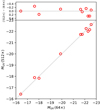 |
Fig. A.1. Absolute UV magnitudes at 1600 Å MUV for the very high-res simulations (512×) vs. production runs (64×). No dust correction has been performed. The top plot shows the difference between the magnitudes. To guide the eye, the grey line shows where MUV(64 × ) = MUV(512 × ). |
Figure A.2 shows the median stellar metallicity [O/H] for nine of the galaxies at 512× vs. 64× resolution. For eight of the galaxies, there is reasonable agreement between 512× and 64× values, with differences being ≲0.2 dex. For the ninth galaxy, the difference is somewhat larger, ∼0.5 dex. This galaxy is small, however, with the 64× version consisting of 69 star particles, so stochastic effects are significant. These results indicate that convergence has been successfully achieved.
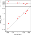 |
Fig. A.2. Median stellar metallicity [O/H] for nine galaxies: very high-resolution simulations (512×) vs. production runs (64×). The top plot shows the difference between the metallicities. To guide the eye, the grey line shows where [O/H](64 × ) = [O/H](512 × ). |
Appendix B: Adding asymmetric uncertainties
On several occasions during this work, it was necessary to add numbers with uncertainties, or errors, not governed by Gaussian probability density functions (PDFs). That is, numbers that are written not as X = x0 ± σ, but as  , where x0 is the central value, and σ− and σ+ are the lower and upper error, respectively. Examples in this work include adding the scatter of the detector limiting magnitudes with the scatter in galaxy fluxes to obtain a PI for the minimum observable mass in Sect. 4.6, adding this PI with the cosmic variance to obtain a PI for the observed number of galaxies in Sect. 4.7, and adding NB and BB magnitudes with errors in Sect. 5.1. If the full PDFs are known, the result X + Y can simply be obtained by convolution or Monte Carlo sampling. In many cases, however, they are not. When only the set {x0, σ−σ+} is known, there cannot be a unique solution, since infinitely many PDFs can be described by the same three numbers.
A widespread yet incorrect approach to this problem is to let the sum of two such numbers be equal to the sum of the central values, with the errors given by the upper and lower errors added in quadrature separately. That is, to set
 (B.1)
(B.1)
This procedure has no statistical justification. That it must be wrong can be seen from considering the central limit theorem: In the limit of many distributions of the same asymmetry, the combined PDF should approach a Gaussian distribution. In contrast, errors added according to Eq. (B.1) never decrease in asymmetry.
Part of the confusion arises from the ambiguity in what represents “the central value”. A common interpretation is the most probable value of the distribution, that is, the mode. An unwary scientist may then think that mode[X + Y]=mode[X]+mode[Y]. But if X and Y are both skewed in the same direction, say towards negative values such that σ− > σ+, the mode will be skewed in the same direction. If x0 represents the mean μ, the combined mean will, indeed, be the sum of the two means, but errors added in quadrature will be even more off. We argue that, for asymmetric errors, a more natural estimator of the central value is the median, and a natural estimator of a CI is the 68% range that is given by the 16th and 84th percentiles. In this case there is equal probability that a number drawn from the PDF lies above and below the central value and, more importantly, one can be sure that the central value lies between the lower and the upper values, which is not necessarily the case for the mode and the mean when dealing with asymmetric PDFs.
A further argument for using the {50, 16, 84} percentiles is that – in contrast to other estimators – they do not care whether the variable in question is linearly or logarithmically distributed (for instance, the median of an ensemble of measured fluxes picks out the same data point as the median of the magnitudes).
A statistical error on x can be thought of as deriving from a nuisance parameter a. If a itself has an uncertainty σa, then in the “normal”, linear case that uncertainty propagates to x as  . Asymmetric errors arise when the relationship between σx and σa is non-linear. As mentioned above, if the full PDFs of X and Y are not known, there is no ‘correct’ solution to the problem. Nevertheless, as described in the following it is possible to construct a method that is a significant improvement over the (standard) quadrature adding. This method is simply a numerical implementation of the technique described by Barlow (2003). We provide a Python function capable of performing such additions online10.
B.1. Error propagation
B.1.1. Piecewise linear error propagation
In the simplest non-linear approach, propagating the uncertainty from a to x knowing only the set {x0, σ−, σ+} can be achieved assuming a piecewise linear dependency. A similar method using a quadratic relationship (not to be confused with ‘addition of errors in quadrature’) has also been implemented in the public code. There is no a priori reason to favour one over the other; the piecewise linear transformation has an unphysical kink, while the quadratic one has a turnover somewhere outside of the 68% CI, but their results are comparable nonetheless (and both much better than the “standard” method).
First, the nuisance parameter a is transformed to a variable u given by a unit Gaussian, while we consider X(u)=x(u)−x(0) as the dependent variable. The function propagating the PDF of the nuisance parameter is then
 (B.2)
(B.2)
A consequence of this transformation is that the expectation value, or the average, of X is no longer equal to the most likely value, but instead given by
 (B.3)
(B.3)
Thus, if X(u) is a non-linear function of u, its expectation ⟨X⟩ is not X(⟨u⟩), and if X(0) is quoted as the central value, it is not the mean. It will still be the median, though, and could as such still be quoted as the central value. The error propagation is illustrated in Fig. B.1.
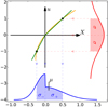 |
Fig. B.1. Error propagation of a nuisance parameter u (red with transparent 1σ confidence interval) to a variable X (blue with 1σ− − 1σ+ confidence intervals) through a piecewise linear relationship (green line). Here, σ− = 0.25 and σ+ = 0.50. A quadratic relationship between u and X is also shown (orange). The mean μ differs from the central value by a factor |

With this transformation we obtain PDFs corresponding to the three-number set, which can then be convolved with the PDF of another three-number set. But convolving two non-Gaussian distributions does not necessarily result in a PDF of the same form as the original functions, as is the case for Gaussian distributions. However, even though the form is not preserved, some things are; the Thiele semi-invariant cumulants (Thiele 1889) still add under convolution. The first three of these are the usual mean (Eq. (B.3)), the variance
 (B.4)
(B.4)
and the unnormalized skewness
![Mathematical equation: $$ \begin{aligned} \gamma&= {\langle X^3 \rangle } - 3{\langle X \rangle }{\langle X^2 \rangle } + 2{\langle X \rangle }^3 \\&= \frac{1}{\sqrt{2\pi }} \left[ 2({\sigma _{+}}^3 - \sigma _{-}^3) - \frac{3}{2} ({\sigma _{+}} - \sigma _{-}) ({\sigma _{+}}^2 + \sigma _{-}^2) \right. \nonumber \\&\quad + \frac{1}{\pi } ({\sigma _{+}} - \sigma _{-})^3 \left. \right]. \nonumber \end{aligned} $$](/articles/aa/full_html/2019/07/aa33645-18/aa33645-18-eq70.gif) (B.5)
(B.5)
The problem of adding n PDFs has now been reformulated so as to find the distribution that has mean, variance, and unnormalized skewness equal to the sums of the indvidual distributions:  , meaning to revert Eqs. (B.3)–(B.5), which express these quantities in terms of σ− and σ+. This must be done numerically. Defining D ≡ σ+ − σ− and
  the equations
 (B.6)
(B.6)
![Mathematical equation: $$ \begin{aligned}&D = \frac{2}{3S} \left[ \sqrt{2\pi }\gamma - D^3 \left(\frac{1}{\pi }-1 \right) \right], \end{aligned} $$](/articles/aa/full_html/2019/07/aa33645-18/aa33645-18-eq74.gif) (B.7)
(B.7)
are solved iteratively, starting with D = 0 (takes only a handful of iterations). The resulting PDF is then given by
 (B.8)
(B.8)
 (B.9)
(B.9)
 (B.10)
where the (biased) mean is calculated through
 (B.11)
and
 (B.12)
is the mean uncertainty.
B.1.2. Quadratic error propagation
The quadratic equivalent of Eq. (B.2) – depicted as the yellow line in Fig. B.1 – is given by
 (B.13)
where
 (B.14)
 (B.15)
The cumulants, that is, the quadratic equivalents of Eqs. (B.3)–(B.5) then become (Barlow 2003)
 (B.16)
 (B.17)
 (B.18)
from which we can solve for x0, σ−, and σ+ using Eqs. (B.8)–(B.10).
B.2. Testing the scheme
B.2.1. Offset of the central value
In order to test the method, we carried out a series of additions of PDFs. The tested functions are of various functional forms (lognormal, loglogistic, Fréchet, and Weibull), and for each pair the value of their parameters are drawn randomly in intervals such that their skewness ranges from zero (symmetric) to ten (highly asymmetric). Their central values and lower and upper uncertainties are calculated, and compared to their “true” values obtained through a convolution of their full PDFs. The result is shown in Fig. B.2 for the central values of the “usual” (left) and the piecewise linear error propagation (right) method.
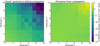 |
Fig. B.2. Offset of the central value x0 from the “true” value x0, true obtained through convolution of 105 random realizations of lognormal, loglogistic, Fréchet, and Weibull distribution, in the case of the “usual”, but wrong, method of adding errors in quadrature (left), and a piecewise linear error propagation (right), as a function of the skewness of the two addends. Here, offset is defined as (x0 − x0, true)/x0, true. The former method is off by a large fraction for relatively small skewnesses, whereas the latter method is correct on the < 1% level even out to skewnesses of 8–9. |
The colour shows the offset of x0 of the two methods from the true result, defined as (x0 − x0, true)/x0, true, as a function of the normalized skewnesses of the two PDFs (defined as the third moment about the mean, divided by the cube of the second moment about the mean). The “usual” method causes an unwanted bias of x0 of > 1% already for small skewnesses of ∼0.5, and for moderate skewnesses of approximately five and above, the bias is > 10%!. This is for adding only two PDFs; if multiple PDFs are added, the bias accumulates, leading to unacceptably large inaccuracies. In contrast, propagating errors through a piecewise linear transformation is accurate on the < 1% level even out to large skewnesses of ∼8
Similar figures can be constructed for the offset of σ− and σ+ and for the quadratic relationship. For the PDFs tested, the piecewise linear method performs slightly better than the quadratic with regards to x0, while the opposite is true for σ− and σ+ (with both methods performing much better than the “usual” method). In this work, because the PIs are somewhat uncertain anyway, we are more concerned with the central value; hence we have chosen to apply the piecewise linear error propagation throughout.
B.2.2. Central limit theorem
As mentioned above, the central limit theorem states that, when adding multiple asymmetric PDFs, their sum should be asymptotically normal, and hence the ratio between the upper and lower errors should approach unity. Conversely, if errors of the same asymmetry are added in quadrature, they stay asymmetric, and the ratio does not change.
To test if our code reproduces this behaviour, we added an increasing number of copies of the same distribution. For a moderate skewness, we arbitrarily chose  . Five different functional forms leading to these asymmetric errors are used as a proxy for how the sum evolves as more terms are added; besides the four used in the previous section, we also use a skewed Gaussian.
Figure B.3 shows in blue how these five different functions first quickly decrease from σ+/σ− = 1.5, then slowly approach σ+/σ− = 1. Both methods (in green and yellow) follow this behaviour nicely. On the other hand, when added in quadrature the ratio stays at σ+/σ− = 1.5.
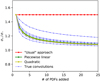 |
Fig. B.3. Decline of the ratio between upper (σ+) and lower (σ−) error when adding multiple PDFs of the same asymmetry, as a function of number of PDFs added. Blue curves show five examples of functional forms that all have |

All Figures
|
Fig. 1. Stellar mass M⋆ as a function of halo mass Mh (SMHM relation) for individual galaxies in the hydro-simulation (black dots), and a power law fit (red) to this distribution. For comparison, a model of the SMHM relation by Behroozi et al. (2013) extrapolated to z = 8.8 is shown in yellow. Shaded areas show the 68% scatter. |
| In the text | |
|
Fig. 2. Total, “intrinsically” emitted Lyα |
| In the text | |
|
Fig. 3. Ratio |
| In the text | |
|
Fig. 4. UV magnitude MUV at 1600 Å as a function of halo mass Mh. For each galaxy the “intrinsic” UV magnitude calculated with STARBURST99 (blue dots) and the reddened magnitudes calculated using the median and 68% scatter of the luminosity-weighted extinction along isotropically distributed sightlines from the star (red dots with error bars) are shown. The red line shows the best fit of the analytical relation in Eq. (16), with the red shaded region showing the prediction interval within which 68% measurements would fall. Only the most massive galaxies are seen to have UV escape fraction significantly below unity, with the red points falling below the blue. |
| In the text | |
|
Fig. 5. Luminosity function Φ at 1600 Å of the simulated galaxies (red solid). The red shaded region shows the 68% spread in Φ, which at the faint end reflects a scatter in the intrinsic UV luminosity, and at the bright also the anisotropic escape of UV radiation due to dust, as well as small-number statistics. Yellow and green dots with error bars show the observed LFs at z ∼ 8 (Bouwens et al. 2015) and z ∼ 10 (Oesch et al. 2018), respectively, with the associated solid lines showing the best-fitting Schechter (1976)-functions. The number of simulated galaxies used for our fit is shown in solid black, with the corresponding numbers on the right y axis. |
| In the text | |
|
Fig. 6. Median spectra of galaxies in various halo mass ranges, normalized to the same stellar mass (109.5 h−1 M⊙), and including the impact of the IGM on the line. The shaded areas show the 68% PIs. Although the median flux in the line hardly rises above the continuum, prominent lines are seen for a significant fraction of the galaxies. Also shown (using the right y axis) is the median transmission of the 16 filters (yellow), and the IGM transmission 𝒯(λ) (black), with the shaded regions showing the 68% scatter. |
| In the text | |
|
Fig. 7. Escape fraction fesc of Lyα as a function of halo mass Mh, defined as the ratio of the number of Lyα photons that make it out through the galaxy to the total number emitted (i.e. if there were no dust and galaxies were isotropic, fesc would be unity in all directions). The red points and the error bars denote the median and the 68% scatter of the six directions along the Cartesian axes, while the blue points show the global average. The extent of the error bars is chiefly dictated by the anisotropy of the ISM, but the scatter in the median values is partly due to only using six directions for the statistics. Only for galaxies above Mh ∼ 1010 h−1 M⊙ does dust play a significant role for the escape fraction. After escaping the galaxy, photons may still be scattered out of the LOS, so the observed fesc would be (much) smaller than these values. To guide the eye, a dashed, grey line is shown at fesc = 1. |
| In the text | |
|
Fig. 8. Measured flux as a function of aperture diameter Dap, normalized to the flux measured at Dap = 2″, for Mh ∼ 1011 h−1 M⊙ (red) and Mh ∼ 1010 h−1 M⊙ (blue) galaxies, with the shaded regions giving the 68% PI. For the Mh ∼ 1011 h−1 M⊙ galaxies, the observed flux for Dap = 2″ is ∼50% compared to Dap → ∞, but since a smaller Dap means less noise, slightly better results are achieved for |
| In the text | |
|
Fig. 9. Flux F measured inside a 1 |
| In the text | |
|
Fig. 10. Cumulative halo mass function (solid red), normalized to the approximate volume surveyed by UltraVISTA. The red shaded region represents the 1σ standard deviation on the number counts resulting from cosmic variance. The dashed blue line shows the minimum observable halo mass (Eq. (19)) in the UltraVISTA survey and the corresponding number of observed galaxies. The blue shaded region shows the 68% PI for this. |
| In the text | |
|
Fig. 11. Lyα LF predicted from our simulations (red with shaded area showing the 68% PI), compared to the three models of Nilsson et al. (2007, described in Sect. 1). Also shown, with the red dashed line, is the Lyα LF predicted from our simulations if we did not take into account RT effects. Additionally, the upper limit LF of Matthee et al. (2014) is shown in green. The grey region marks observational upper limits from Willis & Courbin (2005) and Cuby et al. (2007). |
| In the text | |
|
Fig. 12. Colour-magnitude diagram of the simulated galaxies. Black dots show individual galaxies, with grey error bars showing the 68% scatter for different sightlines. The red line shows a running median (with shaded 68% PI) of the mNB − mBB colour as a function of NB magnitude for all galaxies when we artificially remove their Lyα emission lines. The selection criteria are shown with blue dashed lines; the magnitude threshold is the same as in Sect. 4.6, while the colour threshold is set to mNB − mBB < +0.85, corresponding roughly to the lower limit of the “no Lyα”. Although no galaxy on average falls inside the selection square, the directional variance results in a probability of a few tens of % of being selected, albeit for the brightest galaxies only. |
| In the text | |
|
Fig. 13. Median O VI column density NO VI (red) as a function of impact parameter b, averaged over 6800 sightlines through eight z = 0 disc galaxies simulated using the same code as the one utilized in this work. Shaded regions indicate the 1σ and 2σ deviations from the median, respectively. The observations of “star-forming” galaxies by Tumlinson et al. (2011) are shown by cyan squares. |
| In the text | |
|
Fig. A.1. Absolute UV magnitudes at 1600 Å MUV for the very high-res simulations (512×) vs. production runs (64×). No dust correction has been performed. The top plot shows the difference between the magnitudes. To guide the eye, the grey line shows where MUV(64 × ) = MUV(512 × ). |
| In the text | |
|
Fig. A.2. Median stellar metallicity [O/H] for nine galaxies: very high-resolution simulations (512×) vs. production runs (64×). The top plot shows the difference between the metallicities. To guide the eye, the grey line shows where [O/H](64 × ) = [O/H](512 × ). |
| In the text | |
|
Fig. B.1. Error propagation of a nuisance parameter u (red with transparent 1σ confidence interval) to a variable X (blue with 1σ− − 1σ+ confidence intervals) through a piecewise linear relationship (green line). Here, σ− = 0.25 and σ+ = 0.50. A quadratic relationship between u and X is also shown (orange). The mean μ differs from the central value by a factor |
| In the text | |
|
Fig. B.2. Offset of the central value x0 from the “true” value x0, true obtained through convolution of 105 random realizations of lognormal, loglogistic, Fréchet, and Weibull distribution, in the case of the “usual”, but wrong, method of adding errors in quadrature (left), and a piecewise linear error propagation (right), as a function of the skewness of the two addends. Here, offset is defined as (x0 − x0, true)/x0, true. The former method is off by a large fraction for relatively small skewnesses, whereas the latter method is correct on the < 1% level even out to skewnesses of 8–9. |
| In the text | |
|
Fig. B.3. Decline of the ratio between upper (σ+) and lower (σ−) error when adding multiple PDFs of the same asymmetry, as a function of number of PDFs added. Blue curves show five examples of functional forms that all have |
| In the text | |
Current usage metrics show cumulative count of Article Views (full-text article views including HTML views, PDF and ePub downloads, according to the available data) and Abstracts Views on Vision4Press platform.
Data correspond to usage on the plateform after 2015. The current usage metrics is available 48-96 hours after online publication and is updated daily on week days.
Initial download of the metrics may take a while.