| Issue |
A&A
Volume 622, February 2019
|
|
|---|---|---|
| Article Number | A104 | |
| Number of page(s) | 20 | |
| Section | Cosmology (including clusters of galaxies) | |
| DOI | https://doi.org/10.1051/0004-6361/201732179 | |
| Published online | 05 February 2019 | |
Comparison of the excess mass around CFHTLenS galaxy-pairs to predictions from a semi-analytic model using galaxy-galaxy-galaxy lensing
1
Argelander-Institut für Astronomie, Universität Bonn, Auf dem Hügel 71, 53121 Bonn, Germany
e-mail: This email address is being protected from spambots. You need JavaScript enabled to view it.
2
Exzellenzcluster Universe, Boltzmannstr. 2, 85748 Garching, Germany
3
Ludwig-Maximiliams-Universität, Universitäts-Sternwarte, Scheinerstr. 1, 81679 München, Germany
Received:
26
October
2017
Accepted:
11
December
2018
Abstract
The matter environment of galaxies is connected to the physics of galaxy formation and evolution. In particular, the average matter distribution around galaxy pairs is a strong test for galaxy models. Utilising galaxy-galaxy-galaxy lensing as a direct probe, we map out the distribution of correlated surface mass-density around galaxy pairs in the Canada-France-Hawaii Telescope Lensing Survey (CFHTLenS). We have compared, for the first time, these so-called excess mass maps to predictions provided by a recent semi-analytic model, which is implanted within the dark-matter Millennium Simulation. We analysed galaxies with stellar masses between 109 − 1011 M⊙ in two photometric redshift bins, for lens redshifts z ≲ 0.6. The projected separation of the galaxy pairs ranges between 170 − 300 h−1 kpc, thereby focusing on pairs inside groups and clusters. To allow us a better interpretation of the maps, we discuss the impact of chance pairs, that is galaxy pairs that appear close to each other in projection only. We have introduced an alternative correlation map that is less affected by projection effects but has a lower signal-to-noise ratio. Our tests with synthetic data demonstrate that the patterns observed in both types of maps are essentially produced by correlated pairs which are close in redshift (Δz ≲ 5 × 10⁻³). We also verify the excellent accuracy of the map estimators. In an application to the galaxy samples in the CFHTLenS, we obtain a 3σ − 6σ significant detection of the excess mass and an overall good agreement with the galaxy model predictions. There are, however, a few localised spots in the maps where the observational data disagrees with the model predictions on a ≈3.5σ confidence level. Although we have no strong indications for systematic errors in the maps, this disagreement may be related to the residual B-mode pattern observed in the average of all maps. Alternatively, misaligned galaxy pairs inside dark matter halos or lensing by a misaligned distribution of the intra-cluster gas might also cause the unanticipated bulge in the distribution of the excess mass between lens pairs.
Key words: gravitational lensing: weak / large-scale structure of Universe / cosmology: observations / galaxies: formation / galaxies: evolution / methods: numerical
© ESO 2019
1. Introduction
According to the standard paradigm of galaxy physics, there must exist a strong correlation between the distributions of dark matter and galaxies (Mo et al. 2010). Semi-analytic models (SAMs) of galaxies are one method utilised to simulate the various complexities of galaxy physics by combining analytic prescriptions, where possible, with results from numerical simulations of the cosmological dark-matter density field (e.g. Springel et al. 2005 and Henriques et al. 2015, H15 hereafter). However, while the main physical mechanisms of galaxy evolution seem to be identified by observations, specific details concerning feedback and baryonic physics (of, in particular, star formation) are somewhat unclear. As a result, prescriptions that are encoded in SAMs are frequently phenomenological and employ free parameters calibrated to observables. Typical examples include the stellar-mass function of galaxies or, as for H15, the fraction of quiescent galaxies as function of redshift.
The galaxy-matter correlations as function of galaxy type, cosmic time (redshift), spatial scale, and environment encode useful statistical information about galaxy physics, and they can be used to test SAMs. An important tool for gathering this information is that of weak gravitational lensing, an effect which shears the shapes of distant galaxies (“sources”) through differential light deflection in the presence of a tidal gravitational field between the source and the observer (for a review, see Schneider et al. 2006). Importantly, the shear distortion, as described by the theory of general relativity, does not depend on the nature of the gravitating matter, making lensing an ideal probe for dark-matter physics.
Galaxy-galaxy lensing is one application in weak lensing that considers the correlation between positions of galaxies (lenses) and the shear signal of source galaxies in the background. This is a probe of the radial profile of the surface mass-density of matter around an average lens (e.g. Clampitt et al. 2017; Viola et al. 2015; Choi et al. 2012; Mandelbaum et al. 2006). Galaxy-galaxy-galaxy lensing is a recent extension of the second-order galaxy-galaxy lensing that probes the third-order correlations between the projected matter density and the galaxy number-density with two correlation functions (Simon et al. 2013, 2008; Watts et al. 2005; Schneider & Watts 2005). For the scope of this study, we only work with the lens-lens-shear correlation function and use this correlator synonymously with galaxy-galaxy-galaxy lensing. This kind of statistic is similar to galaxy-galaxy lensing in the sense that it measures the mean tangential shear around pairs of lenses or, after application of a lensing mass-reconstruction, the lensing convergence that is correlated with lens pairs (Simon et al. 2012). Because the lensing convergence is essentially the projected matter density on the sky, the map produced from a galaxy-galaxy-galaxy lensing visualises the typical matter environment of galaxy pairs in projection. With galaxy-galaxy-galaxy lensing being a connected three-point correlation function (by definition), the map shows the convergence in excess of the convergence around two individual galaxies. We therefore refer to this map as “excess mass map”. Since the introduction of galaxy-galaxy-galaxy lensing, alternative lensing measures of mass around average lens pairs have also been proposed and obtained from data, partly to probe the filamentary structure of the cosmic web (Epps & Hudson 2017; Clampitt et al. 2016; Johnston 2006).
As discussed in Saghiha et al. (2012) and recently shown by Saghiha et al. (2017, hereafter S17) galaxy-galaxy-galaxy lensing can test SAMs by comparing model predictions for the average matter density around galaxy pairs to measurements. The analysis in S17 is based on the CFHTLenS1 measurements in Simon et al. (2013, herafter S13), and uses lens galaxies with stellar masses between ∼109 − 1011 M⊙ and redshifts below z ≲ 0.6. S17 find the H15 model to be in good agreement with the CFHTLenS observations, while other models strongly disagree with the data. In addition, S17 argue that, for the same data, galaxy-galaxy-galaxy lensing has more discriminating power in this test than second-order galaxy-galaxy lensing. In particular, the strong dependence on galaxy morphology and galaxy colour makes galaxy-galaxy-galaxy lensing a powerful test for galaxy models.
We revisit the CFHTLenS data and the most promising galaxy model in S17 (i.e. the H15 model) for this paper, in an effort to gain more insight into the matter-galaxy relation on spatial scales of a few 100 h−1 kpc. In particular, we create mass maps such that we are able to probe the matter environment of galaxy pairs on smaller physical scales than the related aperture statistics that are utilised in S17. These maps offer a better intuitive interpretation of the signal, by directly mapping out the average surface-matter density that is correlated with lens pairs for a fixed separation of the pair. Conversely the aperture statistics are useful for quantitative measurements because they are an average of the noisy galaxy-galaxy-galaxy-lensing correlation function for a broad range of separations, closely connected to the angular galaxy-matter bispectrum on the sky. We perform measurements of the excess mass around CFHTLenS galaxy pairs and, in a first study of this kind, compare these maps to the H15 model predictions. Moreover, for future studies, we introduce and investigate a promising new variant of the excess mass which we designate the “pair convergence”. In tests with synthetic data and from theoretical arguments, we find that it is less affected by nonphysical lens pairs that are merely close on the sky in projection (referred to as “chance pairs” in the following).
The structure of the paper is as follows. In Sect. 2, we introduce our notation as well as the definitions of all correlation functions relevant for second-order and third-order galaxy-galaxy lensing. Section 3 introduces the excess mass map and establishes its relation to the correlation function of galaxy-galaxy-galaxy lensing. Importantly, we discuss the effect of chance pairs on the excess map, and we introduce the pair convergence, a variation of the excess mass that is less affected by chance pairs. Our two investigated data sets, the simulated mocks and CFHTLenS data, are briefly described in Sect. 4. In Sect. 5 we outline the two estimators for the excess mass (or the pair convergence). We apply these estimators to CFHTLenS data and simulated H15 data in Sect. 6, verify our computer implementation of the CFHTLenS mapping code, and quantify its accuracy. Finally, in Sect. 7 we discuss our conclusions for the excess mass around CFHTLenS pairs and how they qualitatively compare to the H15 predictions.
2. Formalism
2.1. Lensing notation
Let δm(x) be the fractional density contrast  in the matter-density field ρm(x) relative to the mean density
  at a comoving position x. We define positions x with respect to a fiducial light ray with the observer at the origin (Bartelmann & Schneider 2001). For this, let fK( χ) θ at comoving distance χ be the transverse, comoving separation vector of a neighbour light ray from the fiducial ray, where fK( χ) denotes the comoving angular diameter distance and θ the angular separation of the light ray on the sky. We assume a flat sky and denote angular positions by Cartesian vectors θ = θ1 + iθ2 in a complex notation with origin θ = 0 in the direction of the fiducial ray. For sources distributed along radial distance χ according to the probability density function (PDF) ps( χ), the effective convergence at θ is a projection of δm(x) onto the sky:
 (1)
(1)
 (2)
(2)
where c is the vacuum speed of light, and H0 is the Hubble constant; a( χ) is the scale factor with a( χ)=1 for χ = 0; and χh is the radius of the observable Universe (Schneider et al. 2006). The convergence is related to the (Cartesian) shear field γc(θ) up to a constant κ0 through the convolution integral
 (3)
(3)
with the kernel
 (4)
(4)
(Kaiser & Squires 1993). We call the real part κE(θ) of the convergence the E-mode of the convergence field and the imaginary part κB(θ) its B-mode. In the weak-lensing regime, lens-lens couplings are negligible (Hilbert et al. 2009) so that B-modes serve as indicator of systematic errors for our lensing analysis. In practical studies, we exploit that measurements of the image ellipticity of source galaxies can be converted into unbiased estimates of γc at the positions θ of the sources if |κ| ≪ 1 (e.g. Simon & Schneider 2017). In the following, we therefore denote by ϵi an unbiased estimator of γc(θi) at the position θi of a source galaxy.
We consider the tangential- and cross-shear components γt and γ× of γc(θ) relative to an orientation angle φ, namely we define the φ-rotated shear,
 (5)
(5)
and its decomposition
 (6)
(6)
Also, for mathematical convenience, we denote differences between two vectors θi and θj on the flat sky by
 (7)
(7)
with the polar coordinates θij and φij.
2.2. Galaxy clustering and galaxy-galaxy lensing
In galaxy-galaxy lensing, we correlate positions of lens galaxies with the tangential shear around these galaxies. For this, consider the number density Ng(θ) of lens galaxies on the sky and their density contrast
 (8)
(8)
relative to the mean number density N̅g. Similar to κ(θ), the density contrast κg(θ) constitutes a projection along the line-of-sight θ. Specifically, let δg(x) be the relative fluctuations δng/n̅g in the three dimensional number density of galaxies at a position relative to the fiducial light ray and pd( χ) the PDF of galaxy distances χ inside the observed light cone. Then the density contrast of lenses on the sky is
 (9)
(9)
(e.g. Hoekstra et al. 2002).
Following Peebles (1980), we quantify the second-order angular clustering of lenses by the correlation of two density contrasts with separation ϑ,
 (10)
(10)
Owing to statistical isotropy and homogeneity of the random field δg, the correlation function ω(ϑ) depends only on the separation ϑ of the two points. Likewise, we assume isotropy and homogeneity for the matter-density fluctuations δm so that all following functions that correlate two or more points depend only on the mutual separation of points.
For a cross-correlation of lens positions with the projected matter density, we define the correlation between the number density of lenses and the mean tangential shear
 (11)
(11)
with φ being the polar angle of ϑ = ϑ eiφ. The imaginary part or cross-component  of this correlator vanishes in the statistical average because of a parity invariance of the random fields (Schneider 2003). Physically, galaxy-galaxy lensing probes the (axis-symmetric) profile of the stacked (i.e. ensemble-averaged) convergence
  around lenses at separation ϑ:
 (12)
(12)
(Kaiser 1995).
2.3. Galaxy-galaxy-galaxy lensing
A correlation function similar to galaxy-galaxy lensing can be defined by measuring the average tangential shear at θ3 around a pair of lenses at θ1 and θ2. This is introduced as one of two correlation functions of galaxy-galaxy-galaxy lensing in Schneider & Watts (2005) by
 (13)
(13)
where ϕ3 = φ2 − φ1 denotes the angle spanned by the two separation vectors θ1 − θ3 and θ2 − θ3 with polar angles φ1 and φ2 respectively. Figure 1 sketches the geometry. The tangential shear is thus defined relative to the line that bisects the angle between the two lenses.
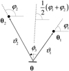 |
Fig. 1. Geometry in the galaxy-galaxy-galaxy lensing correlation function 𝒢 for lenses at θ1 and θ2, and a source at θ3. The separations between source and lenses are ϑ1 and ϑ2. The separations of the lenses is θ12 = |θ1 − θ2|. This figure is copied from Schneider & Watts (2005). |
From a mathematical point of view, 𝒢 is a correlator between the random field κg(θ) at θ1 and θ2, and the random field γc(θ) at θ3. Since both fields vanish on average, i.e., ⟨κg(θ)⟩ = ⟨γc(θ)⟩ = 0 for all θ, the correlation function 𝒢 contains no additive contributions from correlators smaller than third order (the so-called unconnected terms) and thus vanishes for purely Gaussian random fields (e.g. Mo et al. 2010).
3. Mapping of mass correlated with lens pairs
3.1. Definitions of the excess mass
In the case of galaxy-galaxy lensing, the correlator  can be related to the stacked convergence around individual lenses. This is modified in the case of galaxy-galaxy-galaxy lensing, whereby the correlator 𝒢 can now be related to the stacked convergence around individual pairs of lenses (Simon et al. 2008, 2013). We show this by considering first the shear pattern around an average lens pair. Stacking the shear field around two lenses at θ1 and θ2 results in the average
![Mathematical equation: $$ \begin{aligned}&\frac{\left\langle {N_{\rm g}(\boldsymbol{\theta }_1)N_{\rm g}(\boldsymbol{\theta }_2)\gamma _{\rm c}(\boldsymbol{\theta }_3)}\right\rangle }{\left\langle {N_{\rm g}(\boldsymbol{\theta }_1)N_{\rm g}(\boldsymbol{\theta }_2)}\right\rangle } = \frac{\left\langle {[1+\kappa _{\rm g}(\boldsymbol{\theta }_1)][1+\kappa _{\rm g}(\boldsymbol{\theta }_2)]\gamma _{\rm c}(\boldsymbol{\theta }_3)}\right\rangle }{1+\omega (\theta _{12})}\nonumber \\&\,\,= \frac{\left\langle {\kappa _{\rm g}(\boldsymbol{\theta }_1)\,\kappa _{\rm g}(\boldsymbol{\theta }_2)\gamma _{\rm c}(\boldsymbol{\theta }_3)}\right\rangle + \left\langle {\kappa _{\rm g}(\boldsymbol{\theta }_1)\,\gamma _{\rm c}(\boldsymbol{\theta }_3)}\right\rangle +\left\langle {\kappa _{\rm g}(\boldsymbol{\theta }_2)\, \gamma _{\rm c}(\boldsymbol{\theta }_3)}\right\rangle }{1+\omega (\theta _{12})}, \end{aligned} $$](/articles/aa/full_html/2019/02/aa32179-17/aa32179-17-eq19.gif) (14)
(14)
where we have used  , and define θ12 as the separation of the lenses. In order to understand why the left-hand side of Eq. (14) equals the average shear around two lens galaxies, we consider the number-density field of lenses projected on a regular grid with a large number of micro-cells, each with a solid angle σ. We define the micro-cells such that they are sufficiently fine as to contain at most one lens, such that ∫σdσ Ng(θ)=0 or 1. We then have a contribution to ⟨Ng(θ1)Ng(θ2)γc(θ3)⟩ only for ∫σdσ Ng(θ1)=∫σdσ Ng(θ2)=1, while ⟨Ng(θ1)Ng(θ2)⟩ in the denominator is the probability to have a pair of galaxies at θ1 and θ2 at the same time (and is therefore a normalisation factor).
Now, through the definitions Eq. (5) and (11) for galaxy-galaxy lensing we additionally have  and can therefore cast Eq. (14) into
 (15)
(15)
This shows that 𝒢 is, apart from a phase factor, indeed related to the average shear around lens pairs given by the first term on the right-hand side – but rescaled with 1 + ω(θ12) and in excess of the mean shear around individual lenses as given by the two terms that involve  .
.
For the excess mass map, we consider a two-dimensional convergence map  that corresponds to the excess shear in Eq. (15) around lenses at given separation θ12. We construct this map in a specific coordinate frame, for which ϑ is the relative separation from the map centre 𝒪. See the sketch in Fig. 2. The lenses are located at θ1 = −θ12 ex/2 and θ2 = +θ12 ex/2 with ex being a unit vector in the x-direction. Applying the linear Kaiser–Squires transformation in Eq. (3) to Eq. (15) in this coordinate frame yields, up to a constant κ0, a convergence map that can be expanded according to
 (16)
(16)
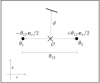 |
Fig. 2. Cartesian coordinate frame for a map of excess mass or the pair convergence. Lenses with separation θ12 are at the positions as indicated by the solid points. A location inside the map is identified by the two-dimensional vector ϑ. |
Here the average convergence  around lens pairs corresponds to the shear stack ⟨NgNgγc⟩/⟨NgNg⟩ in Eq. (15), and the average convergence
  around individual lenses corresponds to the average shear
  , centred on the location of each lens. We emphasise that 1 + ω(θ12) is a constant in this map, and that
  is, by definition of 𝒢, the average convergence around all galaxies in the sample – including those that do not have a partner at separation θ12.
Since the relation between κ(θ) and γc(θ) is only defined up to a constant κ0, we cannot uniquely determine the excess mass map from the excess shear (see Eq. (3)). It is, however, reasonable to assume that  , being the three-point correlation function ⟨κgκgκ⟩, quickly approaches zero for large ϑ which might be used to define κ0. Alternatively, for the maps presented here, we fix κ0 by asserting that
  vanishes when averaged over the entire map area. We will neglect κ0 in the following equations for convenience.
For what follows we also consider the pair convergence of lens pairs as a variant of the excess mass map, which is the straightforward difference signal
 (17)
(17)
between the stacked convergence around lens pairs and the stacked convergence around two individual lenses. Since the excess mass map, originating from the connected correlation function 𝒢, is free of unconnected correlations (by definition), our interpretation is that the excess mass is the connected part of the pair convergence, and the extra term  is the unconnected part of the pair convergence.
While the excess mass exactly vanishes for Gaussian random fields, the pair convergence generally does not; although it is entirely determined by second-order correlations in this case. This can be seen from the definition Eq. (17) of  and Eq. (16) with
  , giving
 (18)
(18)
We visualise the excess mass as a two-dimensional map by plotting either  , or
, or  for the pair convergence, as function of ϑ for a fixed lens-lens separation θ12 and orientation. The resulting maps have two known symmetries (Simon et al. 2008). First, there is a parity symmetry: correlation functions are unchanged under a reflection of shear and the lens density across an axis owing to the parity invariance of cosmological fields (Schneider 2003). As a consequence, quadrants in the maps are statistically consistent when mirrored across the line connecting two lenses. Second, another symmetry is present because we correlate density fluctuations κg at θ1 and θ2 from the same galaxy sample: a permutation of lens indices results in the same correlation function. These symmetries combine to produce, in the absence of noise, an exact reflection symmetry of the map with respect to both the x- and y-axes. We exploit this symmetry to enhance the S/N in the maps by averaging the quadrants inside each map.
Physically, the dimensionless quantities  and
and  are surface-mass densities in units of the (average) critical density
  , defined by
 (19)
(19)
where GN is Newton’s gravitational constant. In our analysis, lenses have a typical distance of zd ≈ 0.4 and sources of zs ≈ 0.93 so that we estimate  as the fiducial value for the critical surface mass density in our analysis below.
3.2. Impact of chance galaxy pairs
The following is a simple discussion exploring the impact of uncorrelated lens pairs on excess mass or pair convergence maps. In the construction of our maps, we select galaxy pairs within a sample by their angular separation θ12 on the sky. Therefore, there will be pairs that are well separated in radial distance from each other, such that third-order correlations involving these are negligible for practical purposes. On the other hand, we will have pairs which have non-negligible third-order correlations with the lensing convergence as they are at similar distance. Naturally, however, making a distinction between what is negligible or otherwise is somewhat arbitrary. Nonetheless we could define a reasonable threshold for the correlation amplitude or a maximum radial separation of galaxies in a pair and use this to restrict our sample to those pairs with higher expected S/N. For the purpose of this simple discussion, however, we assume that we have a sample of lenses with a fraction 1 − ptp of pairs for which a stack of convergence shall be free of any third-order correlations; thus giving the expectation value
 (20)
(20)
These are the “chance pairs”; sources which are pairs only in projection on-sky. The remaining fraction ptp of (physically connected) pairs, to which we refer as “true pairs”, shall have a different yet unspecified stack  that depends in detail on the average surface mass-density around those pairs and the critical density
  at the distance of the pair. The stack around true pairs carries the interesting physical information so that, ideally, we would like to define an excess mass that is independent from chance pairs. This is neither true for an excess mass map nor for a pair convergence map.
We start by exploring the behaviour of pure samples of chance or true pairs. For pure samples of chance pairs (i.e. ptp = 0) the excess mass and pair convergence vanish because mass cannot be correlated with two statistically independent lenses. Indeed, we will find  , ω(θ12)=0, and consequently
  . On the other hand, if we have a pure sample of true pairs (ptp = 1) with a clustering amplitude ωtp (at separation θ12), we will find
 (21)
(21)
for the excess mass. We obtain the equation for  by setting ωtp to zero in Eq. (21).
Usually we have a mixture of chance pairs and true pairs, and the impact of chance pairs on the excess mass is not immediately obvious. To explore this case, let us now assume that 0 < ptp < 1 and that the mean tangential shear  is as unchanged from the pure case. In this mixture, the clustering amplitude is reduced to ω = ptp ωtp, and the convergence stack around all pairs,
 (22)
(22)
is the weighted average of the stacks in the pure samples. Then using Eqs. (20)–(22) in Eq. (16) results, after some algebra, in the excess mass of a mixed sample:
 (23)
(23)
In conclusion, while the presence of chance pairs merely diminishes the overall amplitude of the true pair excess-mass  in the mixture, there is also a second term in the last line of Eq. (23) that changes the overall appearance of the map by adding an extra signal, mainly at the lens positions, that is proportional to the convergence stack around chance pairs.
This extra signal can be avoided in the pair convergence. Namely, by plugging Eqs. (20) and (22) into Eq. (17) we get
 (24)
(24)
for a mixture sample. The presence of chance pairs does at most change the overall amplitude in the pair convergence; each value in the map gives a lower limit to the pair convergence around true pairs inside the brackets of Eq. (24).
4. Data
4.1. The Canada-France-Hawaii Telescope Lensing Survey
The CFHTLenS is a multi-colour, wide-field lensing survey with measurements of galaxy photometry in the five bands u*g′r′i′z′ (AB system), observed as part of the CFHT Legacy Survey Wide (Heymans et al. 2012). The survey covers 154 deg2 of the sky, consisting of four contiguous fields: W1 (≈64 deg2), W2 (≈23 deg2), W3 (≈44 deg2), and W4 (≈23 deg2). The seeing is optimised for lensing measurements in the r′-band and lies typically between 0.″66 − 0.″82; the camera resolution is 0.″187 per CCD pixel. Each field is a mosaic of a set of Megacam pointings with 1 × 1 deg2 field-of-view each. The data reduction uses the processing pipeline THELI (Erben et al. 2013), shear measurements of source galaxies are made using lensfit (Miller et al. 2013), and estimates for galaxy photometric redshifts and stellar masses are obtained using PSF-matched photometry and the computer code BPZ (Hildebrandt et al. 2012, Benitez 2000). The photometric estimator zph for the redshift is the maximum in the posterior redshift distribution of a galaxy. The final galaxy catalogue comprises these physical parameters of 7 × 10⁶ objects2. For our analysis, we use only Megacam pointings that are flagged as “good” for lensing studies. This amounts to roughly 75 per cent of the pointings with an effective area of A ≈ 95 deg2, which we determined by counting the number of unmasked pixels in the mask files of the 129 good pointings. For the selection of lens and source catalogues we follow the criteria in S13, where additionally several tests for systematic errors in the galaxy-galaxy-galaxy lensing measurements (for our samples) have already been performed. S13 also shows plots of the redshift distributions of galaxy samples.
Our source samples are galaxies with i′< 24.7, photometric redshifts of 0.65 ≤ zph < 1.2, and non-vanishing statistical weights wi according to lensfit. This gives roughly 2.2 × 10⁶ sources inside the good pointings, and a mean w-weighted redshift of z̅s ≈ 0.93. The lower limit in zph is chosen to reduce the overlap in redshift between lens and source samples in order to suppress systematic errors in the correlation functions. The effective number density of our sources is  . To correct for the additive and multiplicative bias mi in the estimators ϵi of the shear of the ith source, we follow the instructions in Miller et al. (2013). For this, the correction for mi is easily included in our shear-related estimators by replacing ϵi ↦ ϵi (1 + mi)−1 and wi ↦ wi (1 + mi). We note that we always have mi > −1 (see Appendix A in S13).
For the lens samples, we select galaxies with flux limit i′≤22.5 from two photo-z bins: 0.2 ≤ zph < 0.44 (“low-z”) and 0.44 ≤ zph < 0.6 (“high-z”). In addition, we select galaxies only from the stellar-mass range between 5 × 10⁹ ≤ Msm/M⊙ < 3.2 × 10¹¹ which combines all stellar-mass samples sm1 to sm6 in S13. This selection picks galaxies around the characteristic mass M* ≈ 5 × 10¹⁰ M⊙ of the stellar-mass function (Wright et al. 2017, and references therein). The estimates for stellar masses assume an initial-mass function according to Chabrier (2003) and have a typical RMS error of 0.3 dex (Velander et al. 2014). Counting only good pointings, we have in total 1.8 × 10⁵ galaxies in the low-z sample, yielding N̄g ≈ 0.5 arcmin−2, and 2.5 × 10⁵ galaxies in the high-z sample, N̅g ≈ 0.7 arcmin−2. The mean redshifts are z̅d ≈ 0.35, 0.51 for low-z and high-z respectively. The RMS error of the redshift estimates is σ(z)≈0.04 (1 + z) with an outlier rate of roughly 3%.
The lower limit of allowed stellar masses in addition to the i′≤22.5 flux limit makes our lens sample approximately volume-limited inside the redshift intervals, as can be seen from Fig. A.1. The figure shows absolute rest-frame magnitudes and colours versus redshift for the CFHTLenS galaxies: the blue dots are galaxies with stellar-mass selection, and the orange dots are galaxies without stellar-mass selection. Only the few galaxies that are fainter than Mu ≳ −18.5 or Mg ≳ −19.5 are missing for zph ≳ 0.4. By comparing the distribution of blue and orange points in the colour plots we also see that the stellar-mass selection rejects galaxies bluer than Mg − Mr ≲ 0.3 or Mu − Mg ≲ 0.6 at all redshifts (left column in figure).
4.2. Synthetic lensing data and mock galaxies
Our mock lensing-data are generated by tracing the distortion of light bundles that traverse 64 independent light cones of the N-body Millennium Simulation (Springel et al. 2005; Hilbert et al. 2009). The Millennium Simulation is a purely dark-matter simulation with a spatial (comoving) resolution of 5 h−1 kpc that is sampled by ∼1010 mass particles, populating a cubic region of comoving side length of 500 h−1 Mpc. The fiducial cosmology of the Millenium Simulation has the following parameters: Ωm = 0.25 = 1 − ΩΛ for density parameters of matter and dark energy; Ωb = 0.045 for the baryon density; σ8 = 0.9 for the normalisation of the linear matter power spectrum at z = 0; a Hubble parameter of H0 = h 100 km s−1 Mpc−1 with h = 0.73; and primordial fluctuations as in the Harrison-Zeldovich model. The fiducial cosmology in the Millennium Simulation is somewhat different compared to recent results by the Planck Collaboration XIII (2016). However, we expect that this recent update in cosmological parameters only mildly affects our model predictions, similar to the clustering properties of SAM galaxies in Henriques et al. (2017) where the authors rescale the Millennium Simulation results to the Planck cosmology for a comparison.
Regarding the synthetic lensing data, the simulated light-bundle distortions are an average over source distances with a probability distribution that is the same as that of CFHTLenS sources (see Fig. 5 in S13). Each of the 64 simulated light cones yields a 4 ° ×4° square with information on the theoretical lensing convergence and shear along the line-of-sight at 40962 pixel positions. The total area of the mock data is therefore 1024 deg2. We mainly use the convergence grid for the estimator in Sect. 5.3. Only where we compare the convergence-stack method to the shear-stack method (Sect. 5.1), or where we quantify the model residuals in the maps, do we also generate synthetic shear catalogues. For these catalogues, we uniformly pick random source positions on the grid and assign each the shear value closest to that position as the observed source ellipticity. We therefore do not incorporate any shape noise.
For mock lens galaxies, we apply the H15 SAM-description, adjusted to the fiducial cosmology of the Millennium Simulation. We then follow the steps in S17 (specifically those listed in their Sect. 3.2), to obtain the mock lens samples for low-z and high-z, with a selection function that is consistent with that of galaxies in CFHTLenS, and including an emulation of statistical errors in both stellar masses and photometric redshifts. In particular, the mock samples have redshift distributions that are consistent with the CFHTLenS samples.
5. Estimators of excess mass
We present two estimators for both, the excess mass map (Eq. (16)) and the pair convergence map (Eq. (17)), which aim for different applications. In one version, we stack the shear field around pairs of galaxies and carry out a convergence reconstruction of the stack afterwards. This approach is suitable for observational weak-lensing data where only estimates of (reduced) shear are available for a set of discrete positions of source galaxies. In another version, we stack the convergence on contiguous grids directly, either for quick model predictions of the excess mass or to assess the accuracy of the shear-stacking method.
For practical implementations of both estimators, we note that frequently occurring phase factors e2iφij of separation vectors in our usual complex notation θij = θij eiφij are easily computed by  .
.
5.1. Shear stack
Let  be positions of nd lens galaxies on the sky, and (ϵi, wi,
  ) the details of ns source galaxies with ellipticities ϵi, statistical weights wi, and positions
  . From this, we compute the excess shear in Eq. (15) that is based on both the shear stack around galaxy pairs – the first term of the right-hand side of this equation – and the average shear around individual galaxies, which are the other terms on the right-hand side. Importantly, the excess shear is not identical to the average shear around galaxy pairs; it is usually only a small fraction of the latter.
The overall strategy for an estimator of the excess mass map is: (i) we estimate the excess shear by stacking source ellipticities around lens pairs in an appropriate reference frame and with weights 1 + ω(θ12) (first term in Eq. (15)) and (ii) add the terms that involve  to the stack (other terms); (iii) we apply the Kaiser–Squires inversion, Eq. (3), to obtain the excess mass map in Eq. (16); (iv) finally, we subtract a constant κ0 from the map. The computation of the pair convergence is only slightly different as we explicitly set ω(θ12)≡0 in this procedure. The following describes the details of the stacking and the convergence reconstruction. Therein we assume that estimates of ω(ϑ) and
  are already available; see the following section for estimators of those.
For stacking, we define a two-dimensional grid with Np × Np grid pixels (we choose Np = 200); pixels shall have a square geometry. Each grid cell mn has the vector position pmn = m + i n where (m, n) are its coordinates in a Cartesian stacking frame. Let ( ) be the positions of a selected lens pair ij within the separation bin
  , and
, and  are the details of a source close to the lens pair. We map θ-coordinates to p-coordinates by a rotation αij and scaling |Aij|, both encapsulated inside Aij = |Aij| eiαij, and a translation Bij,
 (25)
(25)
The complex-valued parameters Aij and Bij are determined by the mapping of the two lens positions to the fixed positions  and
and  in the stack,
 (26)
(26)
(see Fig. 3 for an illustration). The positions of sources  are therefore
  in the stacking frame. Additionally, the source ellipticities ϵk have to be rotated by
  in the p-frame. Before mapping ϵk to the stacking frame we subtract off the average shear around each lens position in the θ-frame to obtain the excess shear. The complete stack for the excess shear at the grid pixel mn is then the weighted sum
![Mathematical equation: $$ \begin{aligned}&\Delta \gamma _{mn}= \nonumber \\&\,\,\sum \limits _{i,j,k=1}^{n_{\rm d},n_{\rm s}}\!\! \frac{\Delta _{ijk}^{mn}\ w_k\,\mathrm{e} ^{2\mathrm{i}\alpha _{ij}}}{W_{mn}}\, \Big ([1+\omega (\theta _{ij}^\mathrm{dd})]\,\epsilon _k +\mathrm{e} ^{2\mathrm{i}\varphi _{ik}}\,\overline{\gamma }_{\rm t}(\theta _{ik}^\mathrm{ds}) +\mathrm{e} ^{2\mathrm{i}\varphi _{jk}}\,\overline{\gamma }_{\rm t}(\theta _{jk}^\mathrm{ds})\Big ), \end{aligned} $$](/articles/aa/full_html/2019/02/aa32179-17/aa32179-17-eq73.gif) (27)
(27)
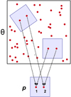 |
Fig. 3. Schematic of the stacking procedure. Positions θ on the sky are mapped to stacking frame positions p defined by the fixed positions of a selected lens pair (red points) in the stacking frame. The stacking-frame positions of the lenses are denoted by |


where the total weight is
 (28)
(28)
and  flags if the source position
  falls within the grid cell mn and
  otherwise; by
  we denote the separation between the lenses i and j, and by
  the difference vector between the lens i and the source k; the angle φik is the polar angle of
  .
.
We then convert the stack Δγmn of excess shear into a map of the excess convergence. Owing to a sparse sampling of the shear stack by discrete source positions around lens pairs, an additional smoothing of this map is required. We apply this smoothing with a kernel K to Δγmn before the conversion to the excess mass map or the pair convergence map, namely by means of
 (29)
(29)
for the Gaussian kernel
 (30)
(30)
which has the kernel size σrms in units of our grid-pixel size. Using the weights Wmn for the smoothing ignores grid pixel with no shear information and gives more weight to pixels with a higher Wmn in the average of neighbouring pixels. We use a smoothing scale of σrms = 4 for our maps.
In the last step, we apply the algorithm by Kaiser & Squires (1993) to  on the grid, employing Fast-Fourier Transformations, to obtain the a smoothed map
  of the excess convergence with a constant offset κ0. The real part in the excess convergence contains the E-mode of the signal, and the imaginary part is the B-mode. Applying the Kaiser–Squires technique on a finite field produces systematic errors which typically have the effect of increasing the signal towards the edges. We therefore remove 50 pixel from the outer edges of the grid in the final map. The inner cropped map has then the dimensions 100× 100 pixel2. The constant offset κ0 depends on the details of the implementation of the Kaiser–Squire algorithm and the number Np of grid pixels. To have consistent maps in the following, we assert that the average excess-convergence over the cropped map has to vanish. We therefore subtract this average from the final map.
5.2. Galaxy-galaxy lensing and lens clustering
The second-order statistics  and ω(ϑ) are estimated from the data by the following standard techniques. For the angular correlation function ω(ϑ) of the lens galaxies, we prepare a mock catalogue with nr uniform random positions within the unmasked region of the survey. We then count the number DD(ϑ; Δϑ) of lens pairs within the separation bin [ϑ − Δϑ/2, ϑ + Δϑ/2), the number of random-galaxy pairs RD(ϑ; Δϑ), and the number of random-random pairs RR(ϑ; Δϑ). For the count rates, we consider all permutations of galaxy and mock positions, which means the total number of DD, RR, and DR for all separations equals nd(nd − 1), nr(nr − 1), and ndnr, respectively. According to Landy & Szalay (1993), we then estimate (for nd, nr ≫ 1)
 (31)
(31)
for the angular clustering of lenses at separation ϑ.
To measure the mean tangential shear  and the cross shear
  within the separation bin [ϑ − Δϑ/2, ϑ + Δϑ/2), we apply the estimator
 (32)
(32)
where  is the phase factor of
  , and Δds(ϑ; Δϑ)=1 for ϑ − Δϑ/2 ≤ θds < ϑ + Δϑ/2 and Δds(ϑ; Δϑ)=0 otherwise (e.g. Bartelmann & Schneider 2001).
Figure 4 is a summary of our measurements of ω(ϑ; Δϑ) and  for both the CFHTLenS data and the H15 galaxy mocks. The measurements are sub-divided into the low-z and high-z redshift bins. We show the tight constraints from the mocks as 2σ regions, and the CFHTLenS measurements as large stars and square with 1σ error bars (obtained by jackknife re-sampling, see Sect. 5.5). The small data points in the bottom panel are the CFHTLenS cross-shear
  of the lens samples, which are plotted as absolute value in the logarithmic plot. The mean of all cross-shear data points is consistent with zero. Regarding a redshift dependence of the measurements, the low-z data points are somewhat higher than the high-z data points for both statistics, a trend which is also predicted by the H15 model. The model predictions for the tangential shear
  are in very good agreement with the CFHTLenS data although the slope for the low-z profile is slightly shallower compared to H15 for ϑ ≲ 5 arcmin. A more detailed comparison of the galaxy-galaxy-lensing signal to H15 can be found in S17.
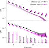 |
Fig. 4. Angular clustering (top panel) and mean tangential shear (bottom panel) of our different lens samples. The large data points show the CFHTLenS measurements for the low-z (stars) and high-z sample (squares) with 1σ error bars, and the coloured regions are 2σ predictions based on the H15 mocks. The grey regions are the predictions for the low-z samples, the magenta regions predict the amplitude of the high-z samples. The small data points with large errors bars at the bottom of the lower panel are the absolute values of the mean cross-shear for the CFHTLenS lenses. |
The amplitude of the angular clustering ω(ϑ) in the model, on the other hand, is about 30% lower than observed. This might partly be explained by a distance distribution pd( χ) of lenses that is actually narrower in CFHTLenS than the assumed distribution in the model. If so, galaxy-galaxy lensing  would be little affected as long as the mean distance of lenses and sources is nevertheless sufficiently accurate. The clustering amplitude ω(ϑ), however, would be affected more strongly because it depends on
  , although it is unlikely that a systematically broadened pd( χ) in the model alone can fully explain the observed discrepancy. This would require the RMS variance of pd( χ) in the model to be biased high by as much as 40%. We obtain this crude estimate by assuming a narrow top-hat shape for pd( χ) with width Δr and centre rc, as in Eq. (11) of Simon (2007). In this case, the amplitude of ω(ϑ) scales with (Δr)−1.
More likely, the disagreement between the clustering of H15 galaxies and CFHTLenS galaxies reflects the current model uncertainties: in particular, Henriques et al. (2017) find a systematically too low amplitude of the galaxy clustering at z = 0.1 in the stellar mass range between  for the H15 model. They find an amplitude too low by ∼20 − 30% at a projected separation between the galaxies of a few 100 h−1 kpc (see their Fig. 13). This comparison to galaxies from the Sloan Digital Sky Survey, albeit at z = 0.1 instead of 0.2 ≲ z ≲ 0.6, is consistent with our finding. The authors argue that the systematic error in the galaxy clustering is related to the treatment of supernova feedback and the gas reincorporation time in the model, affecting the clustering and prevalence of low-mass galaxies. We also refer to the recent work by Cohn (2017) for a thorough discussion on the impact of SAM and simulation parameters on several observational properties of galaxies. As to measurements of galaxy-galaxy-galaxy lensing in this study, we point out that the estimator for the excess mass map uses 1 + ω(ϑ) rather than ω(ϑ) at ϑ ≈ 1 arcmin for which the discrepancy is around 7%, and for the pair convergence map we do not use the angular clustering of lenses at all.
5.3. Convergence stack
In a variant of the previous estimator for maps of the excess mass, we stack the excess convergence  or
or  around lens pairs in simulated data directly. Let
  be the positions of nd lens galaxies and κ(θ) a simulated grid of convergence values. Similar to Sect. 5.1, we use a shear-free affine transformation to map θ positions around a given pair ij of lenses to the stacking frame with coordinates p. The estimation process proceeds in four steps: (i) we stack the convergence around a set of selected lens pairs from the separation bin
  to obtain
  ; (ii) we stack the convergence around individual lenses to obtain
  in the stacking frame; (iii) we estimate 1 + ω averaged for the distribution of lens-lens separations in the sample of selected lens pairs; and (iv) we combine the steps (i) to (iii) to compute the excess mass map
  with an estimate of ω, which is averaged over the distribution of lens-lens separations in the stack. As before, setting ω ≡ 0 in (iii) yields the pair convergence map.
For the steps (i) and (ii), we use square grids with Np × Np pixels and coordinates pmn = m + i n. The lens positions are defined to be at the fixed location  and
and  . Using the definitions Eq. (26) for the parameters of the mapping between the p-frame and the θ-frame for a given lens pair ij, we obtain
 (33)
(33)
for the position θ in the convergence grid that corresponds to the stack position pmn. We then compute the stack  for the grid pixel mn by the average
 (34)
(34)
where  indicates if
  is inside the κ-grid or
  otherwise. In case of
  , we choose the grid point in κ(θ) that is closest to
  .
.
To obtain a map of the average convergence around individual lenses in step (ii), we have to factor in that the convergence around pairs in the stack is differently scaled for any new lens pair in the stack. Therefore, to obtain  for a distribution of scale parameters |Aij| we apply the following technique. For each lens galaxy at
  , we randomly pick a position
  for an “imaginary” uncorrelated lens, where ϕi defines a uniformly random orientation ϕi ∈ [0, 2π) and δθi is a random separation from the ith lens. For δθi, we randomly pick a separation
  from a list of all separations of selected lens pairs in the data. This assures that (ii) consistently uses the same distribution of rescalings |Aij| that are applied in step (i). Since the positions of imaginary lenses are uncorrelated with both κ(θ) and the lens positions, a stack around lens-imaginary pairs yields (on average)
  if the lens is mapped to
  and the imaginary lens mapped to
  ; we obtain
  if we swap the lens positions in the stack. Therefore, by adding the maps for both cases we obtain the stack
  , which justifies the estimator
 (35)
(35)
where  and
and  are defined as before with the exception that we use
  for the position of the second lens in the lens pair ij.
Finally, we combine the information from the previous steps to compute the excess mass around the lens pairs by
![Mathematical equation: $$ \begin{aligned} \overline{\Delta \kappa }_{\rm emm}^{mn}= \Big [1+\omega (\vartheta ;\Delta \vartheta )\Big ]\, \overline{\kappa }_{\rm pair}^{mn}-\overline{\kappa }_{\rm rnd}^{mn}\;. \end{aligned} $$](/articles/aa/full_html/2019/02/aa32179-17/aa32179-17-eq130.gif) (36)
(36)
For a consistent comparison with maps obtained by shear stacking, Sect. 5.1, we smooth the excess mass map with the same kernel as in Eq. (29),
 (37)
(37)
we apply the same cropping, and we subtract the average of  from the cropped map.
5.4. Combining measurements
Our data consist of i = 1…nf separate fields: four fields W1 to W4 for the CFHTLenS data and 64 fields for the synthetic data. Separated fields means here that we ignore contributions from galaxy pairs or triples where not all galaxies are inside the same field. For a combined measurement, we apply the estimators described in the previous sections for each field individually and then average them as described in the following. Our strategy for performing measurements of galaxy-galaxy-galaxy lensing with CFHTLenS data is an improvement in comparison to Simon et al. (2013). In that work, measurements in nf = 129 individual pointings were performed and combined afterwards for a final result. Here, using the continuous fields W1–4, each consisting of many adjacent pointings, allows us to include also galaxy tuples with galaxies from different pointings. We find that this new strategy can enhance the overall S/N in the CFHTLenS maps moderately by 10–30 per cent, depending on the lens samples and their redshift binning.
For a combined estimate of the mean tangential shear  , we imagine the application of Eq. (32) to a merged catalogue of all fields where positions between any pair of galaxies from separate fields are larger than the considered range of ϑ. For this merged catalogue, let
  and
and  be the number of lenses and sources inside field i, and
  the estimator Eq. (32) for galaxies in field i only. We then split the sums over lens-source pairs in Eq. (32) for the merged catalogue into additive contributions from each field to obtain
 (38)
(38)
with the field weights
 (39)
(39)
for the combined estimate. Here  are the statistical weights of sources s in field i, and the flag
  applies to positions in field i only.
For the combined estimate of 1 + ω, we have to determine the count rates DD, DR, and RR in the merged catalogue. To this end, we cannot simply add the count rates of all individual fields. Instead we have to pay attention to the field variations of numbers  of observed galaxies and of unclustered random galaxies in the merged survey. For example, the number of random positions inside field i should depend on the effective area of the field. To quantify this, let pi be the probability that a random position of unclustered galaxies is inside field i, and nr is the total number of random points for all fields; the distribution of mocks in field i complies with the selection function in field i. Only if all fields have the same effective area (or selection function in general), we will find pi = pj = 1/nf for i ≠ j. This, for example, is exactly the case for the 64 fields in our simulated data, and approximately for the 129 CFHTLenS pointings that make up the fields W1–4. For a measurement of the angular clustering of lenses in CFHTLenS, we combine the count rates inside the individual pointings, hence here nf = 129; for all other correlation functions we perform measurements inside the large fields W1-4. Now, counting the total number of random-random pairs in the merged catalogue we find
 (40)
(40)
where  is the count rate RRi in field i normalised with the total number (pinr)2 of random pairs in this field. Conveniently, the value of rri does not depend, on average, on the absolute number of mock positions that we actually in the individual measurement of field i. Therefore, for the combined result of normalised counts
  , we take the average of all individual rri weighted with
  . Similarly, we obtain for the normalised count rate dr = DR/(ndnr) of DR pairs in the merged catalogue
 (41)
(41)
where  is the fraction of galaxies in field i, and dri refers to the normalised rate in field i which, as before, does not depend on the number of mock positions used. Consequently, we compute the combined dr by taking a weighted sum of individual dri. The normalised count
  of DD pairs is
 (42)
(42)
In summary, we compute the count rates (ddi, dri, rri) for each separate field i and then perform the previous weighted sums for the combined rates (dd, dr, rr). By means of the estimator (31), we then get
 (43)
(43)
for the combined clustering amplitude of all fields.
With regard to combining measurements of the shear stacks from a set of nf separate fields we do the following. We apply the estimator Eq. (27) with identical grid parameters to each field i for  and the statistical weights
  . Therein, we constantly use the clustering amplitude 1 + ω as estimated once from the merged catalogue and the measurement of the tangential shear
  in field i. This is consistent with the technique in Simon et al. (2008) but a slight variation compared to Simon et al. (2013) where 1 + ω is measured for each CFHTLenS pointing individually. We then combine the measurements of the excess shear inside the fields into
 (44)
(44)
Finally, we apply the smoothing Eq. (29) to the combined Δγmn and perform the remaining steps in Sect. 5.1 for a combined map of the excess mass.
For a combined measurement of the excess mass map with the convergence-stack technique in Sect. 5.3, we just take the equally weighted average of all grids  obtained from the individual nf = 64 fields. An optimised weighting scheme is not necessary here because this simplistic approach already produces maps with negligible statistical noise for our simulated data.
5.5. Statistical errors
For an estimate of the statistical error in the CFHTLenS maps of the excess mass, we perform the jackknife technique (see e.g. Knight 1999). The basic idea is as follows. Let G(d) be an estimator for some quantity G based on the complete data set d. In our case, G(d) is our estimator for the smoothed excess mass map (or pair convergence map)  at the grid pixel mn, and d comprises the merged catalogue of all separate fields. For the jackknife estimator, we split the complete data d = d1 ∪ d2 ∪ … ∪ dnjn into njn disjoint samples, and we compute a sample {G−i : i = 1…njn} of estimates G−i := G(d ∖ di) based on d without the subset di. We define with
 (45)
(45)
for
 (46)
(46)
the estimator of the jackknife error-variance of G(d). For the following maps, we compute the jackknife error  for every pixel value
  and quote
  for the S/N of a pixel value.
We expect that positional shot-noise and shape noise of the sources as well as cosmic variance are the dominating contributors of statistical noise in our measurement; see, for example, Kilbinger & Schneider (2005) for a discussion of statistical noise in related lensing correlation-functions. For the jackknife scheme, we remove individual pointings di from the merged catalogue; each CFHTLenS pointing has a square geometry and 1 × 1 deg2 area. Since these pointings are significantly larger than our maps with typical angular scale of a few arcmin, we expect a sensible estimate for errors owing to cosmic variance at these scales (Shirasaki et al. 2017).
6. Results
In this section, we present maps of the excess mass  and pair convergence
  for CFHTLenS lenses and for H15 galaxies in our synthetic data. We compute the maps for two photo-z bins and two angular separations of lenses on the sky: the separation bins 40″ ≤ θ12 < 60″ (“close-θ”) and 60″ ≤ θ12 < 80″ (“wide-θ”); and the two redshift bins 0.2 ≤ zph < 0.44 (“low-z”) and 0.44 ≤ zph < 0.6 (“high-z”). We only report E-mode maps in this section; the corresponding B-mode maps can be found in the Appendix. The B-modes are consistent with a vanishing signal. Moreover, we study the impact of a redshift slicing of lenses as means to reduce the fraction of chance pairs in a shear stack.
6.1. Code verification
For Fig. 5, we compare the reconstruction of the excess mass with synthetic data for two different methods: shear stacking (Sect. 5.1) and convergence stacking (Sect. 5.3). For convenience, in the high-z bin we show only the reconstructions for close-θ galaxies. The relative deviations of maps for other samples, including the maps of the pair convergence, are comparable to the single case shown here. The bottom panel employs, for  , the shear-stacking that we apply to the CFHTLenS data. The top panel displays the map
  using direct convergence stacking. Each of the 64 fields contains 2 × 10⁴ sources with no intrinsic shape noise, to reduce the noise in the maps for this comparison. Inside the panels, we indicate the lens positions
  and
and  by black crosses. We overall find an excellent agreement for both approaches, with relative differences usually around five per cent or less, wherever the signal is larger than 5 × 10⁻⁴. However, the differences grow larger close to the lens positions inside the map, as indicated by the contours of
  , shown with the error levels in increments of 10%. Nevertheless, the errors are below 20% except within a couple of pixels separation from the lens positions. Presumably this error is owing to pixellation and binning of the correlation function
  . The 10% error contours at the edges of the map are likely just numerical noise, which becomes relevant for values of
  that are close to zero; the convergence stacking randomly picks a separation to an imaginary lens to subtract second-order correlations from the map. We reiterate that shear stacking is insensitive to constant offsets in κ so that this level of agreement here is only valid for a consistent definition of κ0.
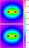 |
Fig. 5. Verification test with simulated data: a comparison of the E-mode excess mass |


6.2. Excess mass maps
The panels A to H in Fig. 6 show the estimated excess mass  , as measured in CFHTLenS (bottom panels C, D, G, H), in comparison to the H15 model predictions (top panels A, B, E, F). The samples are split by column into the low-z and high-z redshift bins; see the labels at the top. The mean redshifts and the angular separations of lenses inside the bins correspond to a range of projected distances between ≈ 170−300 h−1 kpc; the two lens positions are indicated by stars. We quote the distance scale inside the panels. The measurements in CFHTLenS are subject to strong statistical noise due to positional shot-noise and shape noise of the sources. Based on a jackknife resampling of the data, the contour lines encircle areas of 3σ and 5σ significance. Clearly, we find a better than 3σ detection only in the central part of the map, close to and between the lens positions. In comparison, cosmic variance and shot noise by lenses are the only noise components present in the panels for the H15 data. Similar to the H15 model predictions for the aperture statistics in S17, statistical noise is negligible here so that we do not show S/N contours.
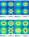 |
Fig. 6. Comparison of the E-mode excess mass (panels A–H) and the pair convergence (panels I–P) between CFHTLenS data (from shear stacks) and the H15 model (from convergence stacks). The maps are arranged in bins of lens redshifts (columns) and projected angular separations of lenses. The mean angular separations for close-θ and wide-θ lenses are converted into projected distances and quoted inside the panels. The lens positions are indicated by stars. The contour lines indicate the significance levels 3σ and 5σ for the CFHTLenS measurements. |
The B-mode of the excess mass in the top panels of Fig. A.2 are indicators of systematic errors. To enhance the significance of the indicators, we also combine the B-mode maps for low-z and high-z in this figure (third column). The consistency of the indicators with random noise supports that systematic errors are negligible inside the maps, at least those that can be detected by B-modes.
Apart from noise in the CFHTLenS maps, we find a good agreement with the predictions for H15 galaxies: a strong concentration of excess mass close to the lens positions and a drop of the signal by about Δκemm = 4 × 10⁻³ from the centre to the outer regions of the maps. This drop corresponds to a change in the excess surface-mass density of  for the fiducial value of
  in Eq. (19). We also observe a tentative indication of a morphological difference between CFHTLenS data and H15, in particular for the panels A vs. C and F vs. H: the excess mass has a bulge-like distribution in vertical direction which is absent in the simulations; the distribution in the simulated maps is more concentrated along the line connecting the lenses inside the map.
Intrigued by this tentative feature in the CFHTLenS data, we produce for a quantitative analysis significance maps of the residuals between CFHTLenS and H15, which are the two panels in Fig. 7. For these two maps, we first compute shear stacks from a synthetic lens and shear catalogue, using exactly the same binning parameters and lens selections as for the CFHTLenS shear stacks. Then we subtract the model shear-stacks from the CFHTLenS shear-stacks, and we then proceed as described in the Sects. 5.1 and 5.5 to produce a S/N map of the residual excess mass. The subtraction of shear steaks avoids the problem of the unknown offset κ0 in the maps. As we are interested in the potential conflicts between H15 and CFHTLenS data, we additionally combine in this process the (residual) shear stacks of the low-z and high-z samples for the same separation bin, giving us two maps instead of four: the left panel for close-θ lenses and the right panel for wide-θ lenses. In these maps, we find an agreement between CFHTLenS and H15 within 3σ with the exceptions of four spots, close to the position of the lenses inside the maps. Here the residuals become negative and attain up to 3.5σ significance (inside the dashed contours). Inside these spots, the CFHTLenS signal is thus lower than the H15 excess mass, which gives rise to the appearance of a squeezed, elongated bulge between the spot positions in the panels C, D, and H of Fig. 6.
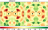 |
Fig. 7. Signal-to-noise ratio of residuals in the CFHTLenS excess mass after subtraction of the shear stacks from the H15 model predictions (E-mode). To increase the significance in both maps, we combine the residual signals from the low-z and high-z samples for the same angular separation. The contours indicate regions of 2σ or 3σ significance; dashed lines are for negative residuals. Left panel: model residuals for the combined close-θ separation bin. Right panel: model residuals for the wide-θ separation bin. |
6.3. Pair convergence maps
In the panels I to P of Fig. 6, we plot the distribution of pair convergence  for our galaxy samples. Again, we have the H15 model predictions in the top panels I, J, M, N, and the corresponding CFHTLenS measurements in the bottom panels K, L, O, and P; the samples are split in redshift and in angular separation of the lenses. We have pointed out in Sect. 3.2 that the distribution of the pair convergence is less affected by chance pairs. However, the then-missing contribution by chance pairs in the maps has the effect that the significance levels for the pair convergence are lower, and the overall amplitude of the signal is also diminished by the fraction of chance pairs in the lens sample. For instance, the significance of the pair convergence between lenses is now just below 3σ for close-θ. In addition, the signal drop Δκ from the map centre to the outer regions is typically smaller for the pair convergence, roughly by a factor of two, namely
  . Again, the B-mode maps in the lower part of Fig. A.2 imply negligible systematic errors.
Moreover, the difference between the signals at the lens positions (stars) and the centre of the maps is smaller than for the excess mass. For the pair convergence of the mock data, we have no pronounced peak at the lens positions but just a diffuse halo in which the lenses are embedded. Although this is similar for the CFHTLenS wide-θ samples (panels O and P), this is not the case for the close-θ samples (panels K and L). This may, in part, be related to the 10–20 per cent inaccuracy of the shear stacking that we find within a few pixels of the lens positions; see Sect. 6.1. More prominently, and different to the H15 prediction, there is a bulge in the distribution of the pair convergence between the galaxies; see in particular the “gummy-bear” like shape in panel P. Similar to the excess mass maps  , this is produced by a relative suppression of signal at the four corners around the lens pair and may be a tentative indication of a disagreement between the H15 prediction and CFHTLenS galaxies. The significance and pattern of residuals is similar to Fig. 7 and not shown here for this reason.
6.4. Fraction of correlated lens pairs
It is interesting to estimate the number of true pairs in the shear stacks of CFHTLenS that are used for Fig. 6. There is, however, no clear distinction between true pairs and chance pairs in reality, in contrast to the idealised discussion in Sect. 3.2. Nevertheless, we can define a statistical measure for the fraction of correlated pairs in a stack by looking at the redshift difference |zi − zj| of the lenses i and j in a pair: galaxies have a typical correlation length of r0 ∼ 5 h−1 Mpc and quickly decorrelate for separations greater than several r0, making them essentially uncorrelated chance pairs. Therefore, as practical measure for the level p̂tp of correlated pairs in a shear stack, we count the number of pairs in a sample and angular separation bin, and we count the expected number nrnd of pairs for lenses with same positions on the sky but uncorrelated redshifts. Based on this we use p̂tp := (npair − nrnd)/npair as a measure for the fraction of excess pairs; uncorrelated lenses, such as chance pairs, would exhibit no excess. In principle, in future studies we could increase the fraction of correlated pairs in a stack by rejecting pairs with |zi − zj|> Δz, provided precise redshift estimators are available (r0 corresponds to Δz ≈ 10−3 for lenses that are on the same line-of-sight). Realistically, a rejection below several 10−3 for Δz is not sensible because peculiar velocities of the galaxies, especially for those in galaxy clusters, spread out the radial distribution of correlated galaxy pairs.
To quantify p̂tp for our CFHTLenS lens pairs and for additional hypothetical Δz-cuts applied to CFHTLenS, we use the H15 lenses (which emulate CFHTLenS but have exact redshifts) in the following way.
-
For different Δz, we count in H15 the number npair of pairs with |zi − zj|≤Δz in the close-θ or wide-θ redshift bin.
-
Then we randomly reassign the redshifts of the lenses in the sample by bootstrapping (with replacement), and we again count the number nrnd of pairs with |zi − zj|≤Δz but in the randomised sample. For the reassignment of redshifts, we only allow as random redshift for a lens k the redshift of another lens l with similar stellar mass. This means, the difference in stellar mass has to be |log10(smk/sml)| ≤ 0.2 dex for the stellar masses smk and sml. We apply this restriction in the bootstrapping because the redshift distribution of lenses is probably slightly dependent on brightness and hence stellar mass, which has to be accounted for in the randomised sample to avoid a bias in nrnd.
The thick black lines in Fig. 8 and the left-hand axis quote our results for p̂tp for lenses in the two redshift bins and the two angular separation bins. This shows that using lens pairs in low-z or high-z with a maximum redshift difference of Δz = 10−3 increases p̂tp to about 32 − 45%, whereas ignoring the lens redshifts (Δz ≫ 1), as we do in the CFHTLenS analysis, reduces p̂tp to below 0.1%. On the other hand, excluding lens pairs with redshift differences greater than Δz reduces the number of pairs in a shear stack by the values that are given by the thin orange lines and the right-hand y-axis. The different line styles belong to the various photo-z and separation bins. We find that a choice of Δz = 0.1 reduces the number of pairs to about 50% of the total number of pairs in low-z or high-z, whereas Δz ∼ 10−3 cuts this number down to below a few per cent. For completeness, we also give the mean redshift difference of lens pairs in H15, which is typically for both separation bins and photo-z bins ⟨|zi − zj|⟩ = 4.0 × 10⁻³, 2.4 × 10⁻², 6.7 × 10⁻² for Δz = 0.01, 0.05, 0.1. In CFHTLenS and our photo-z and separation bins, where we apply no Δz cut, this value is ⟨|zi − zj|⟩ = 0.115.
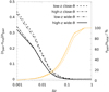 |
Fig. 8. Plot of the estimated fraction (npair − nrnd)/npair of correlated lens pairs in a shear stack (thick lines and y-axis on the left-hand side) for lenses that have redshift difference smaller than Δz (x-axis). We obtain the plotted values for low-z or high-z from H15 by counting the number of pairs npair and the pairs nrnd with randomised redshifts for the angular separations close-θ or wide-θ. In addition, the thin orange lines and the right-hand y-axis show for each separation bin the number of lens pairs npair relative to the total number of pairs, i.e., the npair for Δz ≫ 1. |
6.5. Enriching the levels of correlated lens pairs
The previous section implies that the level of correlated lens pairs in a shear stack may be increased by rejecting pairs that are well separated in redshift. Here we briefly study the impact of this rejection on the maps by using the synthetic data. For this purpose, we focus on the high-z sample and H15 lenses from the close-θ separation bin only; the low-z lenses or the wide-θ separation bin have a qualitatively similar behaviour. We sub-divide the full high-z lens sample into redshift slices of constant width Δz such that lens pairs in each slice have at most a separation of Δz in redshift. For each slice, we stack the shear field around the lenses separately and combine all separate shear stacks into one final shear stack later on, as outlined in Sect. 5.4. In particular, for each individual stack we measure and utilise the mean tangential shear  and angular clustering ω(ϑ) of the lenses in this slice only. We note that this way of rejecting well-separated pairs is wasteful, especially for a very fine slicing, because pairs which have |zi − zj|≤Δz but where each lens resides in a different slice are also rejected. While this is acceptable for our synthetic data, which lacks shape noise, it is sub-optimal for applications to noisy real data. We leave the development of a less wasteful technique to future work.
Figure 9 is a display of the resulting simulated maps for four different slicing parameters Δz = 10−1, 10−2, 5 × 10⁻³, 2 × 10⁻³ and redshifts within the range 0.4 ≤ z ≤ 0.7; the panels A to D are for the excess mass, the panels E to H show the pairs convergence around an average lens pair. We highlight the qualitative changes between the maps when going to a finer slicing by normalising each map to its maximum value. This hides the most prominent effect, namely that the amplitude of the maximum signal in the excess mass maps increases from Δκemm/10−2 = 1.8–10.4 from the coarsest to the finest slicing. This amplitude increase is directly related to the amplitude dependence of the aperture statistics 〈𝒩2 Map〉 on the variance of pd( χ) (Sect. 5.3 in S13). The trend for the pair convergence is less clear: the maximum signal progresses along Δκ/10−3 = 5.3, 8.1, 6.2, 3.2 from Δz = 10−1 to 2 × 10⁻³. The drop in the pair convergence amplitude below Δz ∼ 5 × 10⁻³ despite an increasing p̂tp might indicate that we start to remove lens pairs from the sample that carry a significant correlation signal in the shear stacks. This means, the restrictive slicing might start to affect  in Eq. (24) of the simplified model.
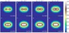 |
Fig. 9. Simulated change in the excess mass (EMM; panels A to D) and pair convergence (PCM; panels E to H) around lens pairs when enriching the level of correlated pairs by further sub-dividing the lens samples into slices with width Δz = 10−1, 10−2, 5 × 10⁻³, 2 × 10⁻³ (left to right). The shear stacks of the slices are combined for the final maps inside the panels. To highlight the relative differences between the maps, all maps are normalised to the maximum signal in the map; the intensity scale varies over the range 10%–100% of the maximum. The maps use the H15 high-z sample and pairs, indicated by the stars, that fall into the close-θ separation bin. |
Apart from the overall change in amplitude the change in the normalised maps is minor for the excess mass (cf. panel A and D) and invisible for the pair convergence. This observation is consistent with the discussion in Sect. 3.2, where we assume a clear-cut dichotomy of correlated “true” and uncorrelated “chance” pairs. In this simplified scenario, the normalised pair convergence is unchanged when increasing the fraction of true pairs, whereas for the excess mass the chance pairs add extra convergence close to the lens positions in the map, weighted by the fraction of true pairs. As the fraction p̂tp increases from panel A to panel D, we therefore anticipate a change in the normalised excess-mass map close to the lens positions, which is indeed visible: we start to see a merging of the halos around the lens positions to one common halo in the excess mass map; similar to what can be seen for the pair convergence.
7. Discussion
Our work is the first direct comparison of the galaxy-galaxy-matter correlation function, measured on real data at arc-minute scales, to the predictions of a galaxy model. We demonstrate that shear-based estimators directly and accurately measure the correlated surface-mass density around physical galaxy pairs, by using a combination of synthetic data, fine redshift slicing of lenses, and direct stacking of convergence. We then apply this method to photo-z binned lenses in real data. Furthermore, we demonstrate that small distortions in the excess mass maps, caused by nonphysical (chance) pairs near the lens positions, can be suppressed by the newly introduced pairs-convergence statistics. We discuss this in depth in the following.
The results for the excess mass maps in the panels C, D, G, and H in Fig. 6 show a clear 3σ − 6σ detection within the inner few 100 h−1 kpc around CFHTLenS galaxy-pairs, and the signal has the expected qualitative behaviour for changes in galaxy separation and redshift. Specifically, our E-mode signal in the excess mass map decreases with lens separation at a fixed redshift (as can be seen by comparing panels C to G and panels D to H) and it decreases with redshift (as seen by comparing panels C to D and panels G to H). Both trends are broadly expected, as the same angular separation of galaxies on the sky at increasing redshift corresponds to larger projected separation, and the three-point correlation function of the matter density field decreases with physical scale; galaxies are essentially tracers of the matter density and therefore their three-point correlations have a similar qualitative behaviour. The signal also varies with the lensing efficiency as expressed by Eq. (19). The relative decrease of  between low-z (z̅d = 0.35) and high-z (z̅d = 0.52) is approximately 15% and thus contributes to a signal decrease. An additional signal decrease towards higher redshift may be given by gravitational growth of structure which amplifies the non-Gaussianity of the density fields with time. Finally, the consistency of explicit convergence stacking and shear stacking with synthetic data in Sect. 6.1 shows that the CFHTLenS maps can be interpreted as maps of excess convergence that is correlated with galaxy pairs, in concordance with the theory presented in Sect. 3. In addition, Fig. 9 underscores that the characteristic patterns in the maps originate from physically close lens pairs that have Δz ≲ 5 × 10⁻³, even if the majority of pairs are chance pairs as in our CFHTLenS data (Fig. 8).
We have also introduced the pair convergence  as alternative measure of the excess mass
  to suppress the contamination by chance (uncorrelated) pairs in the correlation statistics, and we detect it with a significance of 3σ − 4σ for our CFHTLenS lenses. The maps are shown in panels K, L, O, and P in Fig. 6. As to the motivation for an alternative measure, our mapping technique of the excess mass stacks shear around galaxy pairs, within a given separation interval on the sky. However, the vast majority of selected pairs are actually well separated in physical distance; they are uncorrelated chance pairs. In fact, in each of the low-z and high-z samples fewer than 5% of our lens pairs have redshift differences of Δz = 5 × 10⁻³ or less (see Fig. 8). Fortunately, the main effect of the chance pairs is to dilute the correlation signal and to slightly distort the excess mass
  close to the lens positions inside the map (see Sect. 3.2). It may be desired to remove this distortion by rejecting chance pairs in the stack, which, however, is difficult owing to the typical errors σ(z)≈0.04 of the photometric-redshift estimations in CFHTLenS. Therefore, we have defined by Eq. (17) the slightly modified statistic of the pair convergence
  which is not distorted by uncorrelated pairs (but also has a somewhat different meaning). On the other hand, the (weakly distorted) excess mass
  may be, after all, mathematically preferable because it is only a function of the matter-galaxy bispectrum and thus exactly vanishes for Gaussian density fields (Schneider & Watts 2005).
As expected from the recent work by S17, there is a good agreement between the H15 predictions for the excess mass and our measurements with CFHTLenS data, although we find some evidence for morphological differences to the SAM predictions, especially for the pair convergence. S17 measured, among other things: the 𝒢-related aperture statistics 〈𝒩2Map〉(θap) for angular scales θap between 1 and 10 arcmin, for their galaxy samples sm1 to sm6 in both the low-z and high-z redshift bins, and they find a good match between observations and the H15 model for all stellar-mass samples, reported in their Table 6. Therefore, we expect that the H15 excess-mass maps should also agree well with the measurements despite probing somewhat smaller angular scales. Indeed the H15 distribution of excess mass and its overall amplitude is consistent with CFHTLenS, as can be seen from panels A to H in the Fig. 6. With regard to possible differences between the H15 predictions and CFHTLenS, we notice a bulge of excess mass in the vertical direction at the centre the excess-mass maps. This can especially be seen in the panels H and P in comparison to the models F and N, respectively, in Fig. 6. To quantify the differences, we produce two maps of model residuals in Fig. 7 where we find good agreement between model and CFHTLenS almost everywhere inside the maps within 3σ confidence, with the exceptions of four spots of negative residuals with approximately 3.5σ significance (close-θ in the left panel) and 3σ significance (wide-θ in the right panel). The corresponding map for the pair convergence is similar and therefore not shown. The suppression of the correlation signal at these spots produces the elongated bulge of excess mass perpendicular to the orientation of the lens pair.
We have taken precautions to suppress spurious signals in the lensing maps owing to intrinsic alignments of sources, and have performed basic tests to confirm that the bulge feature is not induced by a trivial systematic error. For overlapping distance distributions of lenses and sources, we may find sources at lens distances. In this case, correlations of intrinsic source ellipticities with the matter density around lens pairs can add signal to our maps of the excess mass or pair convergence. Although this effect is currently not well studied, S13 argue that the alignment signal can be suppressed by reducing the overlapping area A of pd(z) and ps(z), where A := ∫dz a(z) is the integral over a(z)=min{pd(z),ps(z)}. Using photometric redshifts, our separation of lens and source distributions is not perfect, but the overlap of the distributions is small: approximately A = 4% for low-z and A = 12% for high-z (S13). In particular, the bulge is still visible for panel H in Fig. 6 despite the small 4% overlap for low-z. Therefore, the bulge is probably unrelated to intrinsic alignments. Furthermore, numerical artefacts in the computer code that produce a bulge feature are also unlikely as can be seen by the verification test in Fig. 5. Here systematic errors are present close to the lens positions only. We note that masking of data is not included in the verification test, however this is not a plausible cause of this effect: mask-related systematic errors should not have a preferred map direction, unless the orientation of galaxy pairs at zd ≳ 0.2 is correlated with the orientation of mask features. As masking is mainly produced by satellite tracks, stars, instrumental CCD effects, cosmic rays, or low-redshift galaxies (Erben et al. 2013), this is unlikely. As another possible systematic effect, we test if blending of galaxy images could bias the shear estimates of CFHTLenS sources and affect the excess maps (Miller et al. 2013). For the test, we have produced new maps with same binning parameters as in the panels A to H in Fig. 6, although now rejecting sources within nine arcsec of a lens galaxy for the shear stack. We find no significant difference to the maps without rejection, and, in particular, the bulge feature persists (not shown to save space). Finally, we stack the shear patterns of all panels K, L, O, and P in Fig. 6 to investigate a possible residual pattern in the B-modes that is correlated with the prominent bulge feature in the pair convergence maps. We overlay the B-mode signal as black contours in Fig. A.3 on top of the combined E-mode. The merged stacks of all lenses clearly show the bulge at the centre, although the B-mode amplitude is typically below 5 × 10⁻⁴ near the bulge and thus small compared to the E-mode signal. However, the B-mode signal is correlated with the bulge, and extends to larger separations in the vertical direction at the positions of the lenses (crosses) compared to its vertical extension at the bulge location. This may equally be a coincidence or an indication of a systematic effect for the bulge appearance. Nonetheless, a clear interpretation of an alignment between a residual B-mode signal and the E-mode bulge is difficult, since we lack a model for systematic errors here that convincingly connects both.
On the speculative side, if the bulge in the distribution of excess mass is indeed a physical effect it could point to missing elements in the dark-matter simulation or the SAM galaxy model (or the similar SAMs in S17) used for this study. One conceivable element might be the extra lensing signal caused by the intra-cluster medium (ICM) that constitutes 10 − 15% of the mass of matter halos in galaxy clusters. On the one hand, if the ICM distribution is aligned with the distribution of dark matter, there will be no qualitative change in the distribution of excess mass, because additional gravitational lensing by the ICM only rescales the dominating dark-matter signal. On the other hand, a misalignment between the ICM and the dark-matter distribution might produce a weak bulge feature if the ICM density is increased perpendicular to the lens-lens axis. This could be tested with cosmological simulations that include baryons, or analytically with a halo model that includes misaligned mass-distributions (e.g. Cooray & Sheth 2002). Similarly, we could imagine a bulge feature being induced by a statistical misalignment between the orientation of lens pairs and the orientation of their parent halo. As an extreme example, one might consider a distribution of galaxies distributed in the equatorial plane of a prolate halo: stacking the surface matter-density of the halo around pairs of these galaxies would result in an elongated excess signal perpendicular to the orientation of lens pairs. This too could be tested with simulations or a halo model by populating non-spherical dark-matter halos with a misaligned galaxy distribution.
By selecting galaxy pairs with projected separations of around 250 h−1 kpc our analysis probes the matter environment of pairs inside galaxy groups and clusters. While this regime is of particular interest to test the predictive power of galaxy models, such as H15, future applications this probe may also be utilised to analyse the filamentary large-scale distribution of matter around physical pairs. To this end, future works should aim to map the pair convergence around luminous red galaxies at ∼10 h−1 Mpc separation, in a way that is similar to that presented in Epps & Hudson (2017) and Clampitt et al. (2016), where successful detections have been reported.
Acknowledgments
We thank the anonymous referee for the thoughtful comments. This work has been supported by the Deutsche Forschungsgemeinschaft through the project SI 1769/1-1 and through the Collaborative Research Center TR33 “The Dark Universe”. Patrick Simon also acknowledges support from the German Federal Ministry for Economic Affairs and Energy (BMWi) provided via DLR under project no. 50QE1103. Stefan Hilbert acknowledges support by the DFG cluster of excellence “Origin and Structure of the Universe” (http://www.universe-cluster.de/).
References
- Bartelmann, M., & Schneider, P. 2001, Phys. Rep., 340, 291 [NASA ADS] [CrossRef] [Google Scholar]
- Benitez, N. 2000, ApJ, 536, 571 [NASA ADS] [CrossRef] [Google Scholar]
- Chabrier, G. 2003, PASP, 115, 763 [NASA ADS] [CrossRef] [Google Scholar]
- Choi, A., Tyson, J. A., Morrison, C. B., et al. 2012, ApJ, 759, 101 [NASA ADS] [CrossRef] [Google Scholar]
- Clampitt, J., Miyatake, H., Jain, B., & Takada, M. 2016, MNRAS, 457, 2391 [NASA ADS] [CrossRef] [Google Scholar]
- Clampitt, J., Sánchez, C., Kwan, J., et al. 2017, MNRAS, 465, 4204 [NASA ADS] [CrossRef] [Google Scholar]
- Cohn, J. D. 2017, MNRAS, 466, 2718 [NASA ADS] [CrossRef] [Google Scholar]
- Cooray, A., & Sheth, R. 2002, Phys. Rep., 372, 1 [NASA ADS] [CrossRef] [Google Scholar]
- Epps, S. D., & Hudson, M. J. 2017, MNRAS, 468, 2605 [NASA ADS] [CrossRef] [Google Scholar]
- Erben, T., Hildebrandt, H., Miller, L., et al. 2013, MNRAS, 433, 2545 [NASA ADS] [CrossRef] [Google Scholar]
- Henriques, B. M. B., White, S. D. M., Thomas, P. A., et al. 2015, MNRAS, 451, 2663 [NASA ADS] [CrossRef] [Google Scholar]
- Henriques, B. M. B., White, S. D. M., Thomas, P. A., et al. 2017, MNRAS, 469, 2626 [Google Scholar]
- Heymans, C., Van Waerbeke, L., Miller, L., et al. 2012, MNRAS, 427, 146 [NASA ADS] [CrossRef] [Google Scholar]
- Hilbert, S., Hartlap, J., White, S. D. M., & Schneider, P. 2009, A&A, 499, 31 [NASA ADS] [CrossRef] [EDP Sciences] [Google Scholar]
- Hildebrandt, H., Erben, T., Kuijken, K., et al. 2012, MNRAS, 421, 2355 [NASA ADS] [CrossRef] [Google Scholar]
- Hoekstra, H., van Waerbeke, L., Gladders, M. D., Mellier, Y., & Yee, H. K. C. 2002, ApJ, 577, 604 [NASA ADS] [CrossRef] [Google Scholar]
- Johnston, D. E. 2006, MNRAS, 367, 1222 [NASA ADS] [CrossRef] [Google Scholar]
- Kaiser, N. 1995, ApJ, 439, L1 [NASA ADS] [CrossRef] [Google Scholar]
- Kaiser, N., & Squires, G. 1993, ApJ, 404, 441 [NASA ADS] [CrossRef] [Google Scholar]
- Kilbinger, M., & Schneider, P. 2005, A&A, 442, 69 [NASA ADS] [CrossRef] [EDP Sciences] [Google Scholar]
- Knight, K. 1999, Mathematical Statistics, Chapman& Hall/CRC Texts in Statistical Science, (CRC Press) [Google Scholar]
- Landy, S. D., & Szalay, A. S. 1993, ApJ, 412, 64 [NASA ADS] [CrossRef] [Google Scholar]
- Mandelbaum, R., Seljak, U., Kauffmann, G., Hirata, C. M., & Brinkmann, J. 2006, MNRAS, 368, 715 [Google Scholar]
- Miller, L., Heymans, C., Kitching, T. D., et al. 2013, MNRAS, 429, 2858 [Google Scholar]
- Mo, H., van den Bosch, F. C., & White, S. 2010, Galaxy Formation and Evolution (Cambridge: Cambridge University Press) [Google Scholar]
- Peebles, P. J. E. 1980, The large-scale structure of the universe (Princeton, NJ: Princeton University Press) [Google Scholar]
- Planck Collaboration XIII. 2016, A&A, 594, A13 [NASA ADS] [CrossRef] [EDP Sciences] [Google Scholar]
- Saghiha, H., Hilbert, S., Schneider, P., & Simon, P. 2012, A&A, 547, A77 [NASA ADS] [CrossRef] [EDP Sciences] [Google Scholar]
- Saghiha, H., Simon, P., Schneider, P., & Hilbert, S. 2017, A&A, 601, A98 [NASA ADS] [CrossRef] [EDP Sciences] [Google Scholar]
- Schneider, P. 2003, A&A, 408, 829 [NASA ADS] [CrossRef] [EDP Sciences] [Google Scholar]
- Schneider, P., & Watts, P. 2005, A&A, 432, 783 [NASA ADS] [CrossRef] [EDP Sciences] [Google Scholar]
- Schneider, P., Kochanek, C., & Wambsganss, J. 2006, Gravitational lensing: strong, weak and micro, Saas-Fee Advanced Course: Swiss Society for Astrophysics and Astronomy (Berlin: Springer) [Google Scholar]
- Shirasaki, M., Takada, M., Miyatake, H., et al. 2017, MNRAS, 470, 3476 [NASA ADS] [CrossRef] [Google Scholar]
- Simon, P. 2007, A&A, 473, 711 [NASA ADS] [CrossRef] [EDP Sciences] [Google Scholar]
- Simon, P., & Schneider, P. 2017, A&A, 604, A109 [NASA ADS] [CrossRef] [EDP Sciences] [Google Scholar]
- Simon, P., Watts, P., Schneider, P., et al. 2008, A&A, 479, 655 [NASA ADS] [CrossRef] [EDP Sciences] [Google Scholar]
- Simon, P., Schneider, P., & Kübler, D. 2012, A&A, 548, A102 [NASA ADS] [CrossRef] [EDP Sciences] [Google Scholar]
- Simon, P., Erben, T., Schneider, P., et al. 2013, MNRAS, 430, 2476 [NASA ADS] [CrossRef] [EDP Sciences] [Google Scholar]
- Springel, V., White, S. D. M., Jenkins, A., et al. 2005, Nature, 435, 629 [NASA ADS] [CrossRef] [PubMed] [Google Scholar]
- Velander, M., van Uitert, E., Hoekstra, H., et al. 2014, MNRAS, 437, 2111 [NASA ADS] [CrossRef] [Google Scholar]
- Viola, M., Cacciato, M., Brouwer, M., et al. 2015, MNRAS, 452, 3529 [CrossRef] [Google Scholar]
- Watts, P., & Schneider, P. 2005, in Gravitational Lensing Impact on Cosmology, eds. Y. Mellier, & G. Meylan (Cambridge: Cambridge University Press), IAU Symp., 225 [Google Scholar]
- Wright, A. H., Robotham, A. S. G., Driver, S. P., et al. 2017, MNRAS, 470, 283 [NASA ADS] [CrossRef] [Google Scholar]
Appendix A: Additional figures
As additional characterisation of the population of lens galaxies in our analysis of the excess mass, we plot in Fig. A.1 their distribution of absolute rest-frame magnitudes or colours for (photometric) redshifts zph between 0.2 and 0.6. Moreover, Figs. A.2 and A.3 are maps of the B-mode signal of the excess mass which are a diagnostic for systematic errors in the correlation signal.
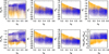 |
Fig. A.1. Properties of the targeted sample of lens galaxies in the lensing analysis. Shown are scatter plots of absolute rest-frame u*g′r′i′z′-magnitudes, colours, and stellar masses versus the photometric redshift zph (BPZ) of the CFHTLenS galaxies with flux limit i′≤22.5 in the stellar-mass interval 5 × 10⁹ ≤ Msm < 3.2 × 10¹¹ M⊙ (blue dots). The brighter orange dots show the scatter for lenses for all stellar masses which are clearly flux limited at higher redshifts zph. The data points are from galaxies in the field W1 only; other fields look similar. |
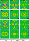 |
Fig. A.2. B-mode maps of the excess mass around CFHTLenS galaxy pairs for the excess mass (top panels) and the pair convergence (bottom panels). The angular scale and redshift selections are indicated inside the panels. The crosses show the lens positions inside the map. The contours indicate regions with significance greater or equal 3σ. |
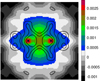 |
Fig. A.3. Average of all pair-convergence maps in Fig. 6, panels K, L, O, and P, and the corresponding B-mode maps by combining all shear stacks used for that figure. The E-mode is shown here as intensity scale, the B-mode is shown as overlay of iso-contours for the levels 2 × 10⁻⁴, 4 × 10⁻⁴, and 6 × 10⁻⁴. |
All Figures
|
Fig. 1. Geometry in the galaxy-galaxy-galaxy lensing correlation function 𝒢 for lenses at θ1 and θ2, and a source at θ3. The separations between source and lenses are ϑ1 and ϑ2. The separations of the lenses is θ12 = |θ1 − θ2|. This figure is copied from Schneider & Watts (2005). |
| In the text | |
|
Fig. 2. Cartesian coordinate frame for a map of excess mass or the pair convergence. Lenses with separation θ12 are at the positions as indicated by the solid points. A location inside the map is identified by the two-dimensional vector ϑ. |
| In the text | |
|
Fig. 3. Schematic of the stacking procedure. Positions θ on the sky are mapped to stacking frame positions p defined by the fixed positions of a selected lens pair (red points) in the stacking frame. The stacking-frame positions of the lenses are denoted by |
| In the text | |
|
Fig. 4. Angular clustering (top panel) and mean tangential shear (bottom panel) of our different lens samples. The large data points show the CFHTLenS measurements for the low-z (stars) and high-z sample (squares) with 1σ error bars, and the coloured regions are 2σ predictions based on the H15 mocks. The grey regions are the predictions for the low-z samples, the magenta regions predict the amplitude of the high-z samples. The small data points with large errors bars at the bottom of the lower panel are the absolute values of the mean cross-shear for the CFHTLenS lenses. |
| In the text | |
|
Fig. 5. Verification test with simulated data: a comparison of the E-mode excess mass |
| In the text | |
|
Fig. 6. Comparison of the E-mode excess mass (panels A–H) and the pair convergence (panels I–P) between CFHTLenS data (from shear stacks) and the H15 model (from convergence stacks). The maps are arranged in bins of lens redshifts (columns) and projected angular separations of lenses. The mean angular separations for close-θ and wide-θ lenses are converted into projected distances and quoted inside the panels. The lens positions are indicated by stars. The contour lines indicate the significance levels 3σ and 5σ for the CFHTLenS measurements. |
| In the text | |
|
Fig. 7. Signal-to-noise ratio of residuals in the CFHTLenS excess mass after subtraction of the shear stacks from the H15 model predictions (E-mode). To increase the significance in both maps, we combine the residual signals from the low-z and high-z samples for the same angular separation. The contours indicate regions of 2σ or 3σ significance; dashed lines are for negative residuals. Left panel: model residuals for the combined close-θ separation bin. Right panel: model residuals for the wide-θ separation bin. |
| In the text | |
|
Fig. 8. Plot of the estimated fraction (npair − nrnd)/npair of correlated lens pairs in a shear stack (thick lines and y-axis on the left-hand side) for lenses that have redshift difference smaller than Δz (x-axis). We obtain the plotted values for low-z or high-z from H15 by counting the number of pairs npair and the pairs nrnd with randomised redshifts for the angular separations close-θ or wide-θ. In addition, the thin orange lines and the right-hand y-axis show for each separation bin the number of lens pairs npair relative to the total number of pairs, i.e., the npair for Δz ≫ 1. |
| In the text | |
|
Fig. 9. Simulated change in the excess mass (EMM; panels A to D) and pair convergence (PCM; panels E to H) around lens pairs when enriching the level of correlated pairs by further sub-dividing the lens samples into slices with width Δz = 10−1, 10−2, 5 × 10⁻³, 2 × 10⁻³ (left to right). The shear stacks of the slices are combined for the final maps inside the panels. To highlight the relative differences between the maps, all maps are normalised to the maximum signal in the map; the intensity scale varies over the range 10%–100% of the maximum. The maps use the H15 high-z sample and pairs, indicated by the stars, that fall into the close-θ separation bin. |
| In the text | |
|
Fig. A.1. Properties of the targeted sample of lens galaxies in the lensing analysis. Shown are scatter plots of absolute rest-frame u*g′r′i′z′-magnitudes, colours, and stellar masses versus the photometric redshift zph (BPZ) of the CFHTLenS galaxies with flux limit i′≤22.5 in the stellar-mass interval 5 × 10⁹ ≤ Msm < 3.2 × 10¹¹ M⊙ (blue dots). The brighter orange dots show the scatter for lenses for all stellar masses which are clearly flux limited at higher redshifts zph. The data points are from galaxies in the field W1 only; other fields look similar. |
| In the text | |
|
Fig. A.2. B-mode maps of the excess mass around CFHTLenS galaxy pairs for the excess mass (top panels) and the pair convergence (bottom panels). The angular scale and redshift selections are indicated inside the panels. The crosses show the lens positions inside the map. The contours indicate regions with significance greater or equal 3σ. |
| In the text | |
|
Fig. A.3. Average of all pair-convergence maps in Fig. 6, panels K, L, O, and P, and the corresponding B-mode maps by combining all shear stacks used for that figure. The E-mode is shown here as intensity scale, the B-mode is shown as overlay of iso-contours for the levels 2 × 10⁻⁴, 4 × 10⁻⁴, and 6 × 10⁻⁴. |
| In the text | |
Current usage metrics show cumulative count of Article Views (full-text article views including HTML views, PDF and ePub downloads, according to the available data) and Abstracts Views on Vision4Press platform.
Data correspond to usage on the plateform after 2015. The current usage metrics is available 48-96 hours after online publication and is updated daily on week days.
Initial download of the metrics may take a while.