| Issue |
A&A
Volume 621, January 2019
|
|
|---|---|---|
| Article Number | A113 | |
| Number of page(s) | 19 | |
| Section | Planets and planetary systems | |
| DOI | https://doi.org/10.1051/0004-6361/201833014 | |
| Published online | 15 January 2019 | |
Analysis of a long-lived, two-cell lightning storm on Saturn★
1
Space Research Institute, Austrian Academy of Sciences,
Schmiedlstr. 6,
8042 Graz, Austria
e-mail: georg.fischer@oeaw.ac.at
2
Institute of Physics, University of Graz,
Universitätsplatz 5,
8010 Graz, Austria
3
LESIA, Observatoire de Paris, CNRS, PSL, UPMC/SU, UPD,
5 Place Jules Janssen,
92195 Meudon, France
4
Commission des observations planétaires, Société Astronomique de France, Paris, France
5
Geological and Planetary Sciences, 150–21, California Institute of Technology,
Pasadena,
CA 91125, USA
6
Department of Physics and Astronomy, The University of Iowa,
Iowa City,
IA 52242, USA
Received:
13
March
2018
Accepted:
14
November
2018
Lightning storms in Saturn’s atmosphere can last for a few days up to several months. In this paper we analyze a lightning storm that raged for seven and a half months at a planetocentric latitude of 35° south from the end of November 2007 until mid-July 2008. Thunderstorms observed by the Cassini spacecraft before this time were characterized by a single convective storm region of ~2000 km in size, but this storm developed two distinct convective storm cells at the same latitude separated by ~25° in longitude. The second storm cell developed in March 2008, and the entire two-cell convective system was moving with a westward drift velocity of about 0.35 deg per day, which differs from the zonal wind speed. An exhaustive data analysis shows that the storm system produced ~277000 lightning events termed Saturn electrostatic discharges (SEDs) that were detected by Cassini’s Radio and Plasma Wave Science (RPWS) instrument, and they occurred in 439 storm episodes. We analyzed the SED intensity distributions, the SED polarization, the burst rates, and the burst and episode durations.
During this storm Cassini made several orbits around Saturn and observed the SEDs from all local times. A comparison with optical observations shows that SEDs can be detected when the storm is still beyond the visible horizon. We qualitatively describe this so-called over-the-horizon effect which is thought to be due to a temporary trapping of SED radio waves below Saturn’s ionosphere. We also describe the first occurrence of so-called SED pre- and post-episodes, which occur in a limited frequency range around 4 MHz separated from the main episode. Pre- and post-episodes were mostly observed by Cassini located at local noon, and should be a manifestation of an extreme over-the-horizon effect. Combined radio and imaging observations suggest that some decreases in SED activity are caused by splitting of the thunderstorm into a bright cloud and a dark oval.
Key words: planets and satellites: atmospheres / planets and satellites: gaseous planets / methods: data analysis
Table C.1 is only available at the CDS via anonymous ftp to cdsarc.u-strasbg.fr (130.79.128.5) or via http://cdsarc.u-strasbg.fr/viz-bin/qcat?J/A+A/621/A113
© ESO 2019
1 Introduction
Radio emissions from Saturn lightning were detected by both Voyagers (Warwick et al. 1981, 1982) and by the Cassini spacecraft (Fischer et al. 2006), and the strong intensities of Saturn lightning also led to a detection with radio telescopes on Earth (Zakharenko et al. 2012; Konovalenko et al. 2013). The Saturn electrostatic discharges (SEDs) are typically 10 000 times stronger than terrestrial “sferics” (short for radio signals from atmospheric lightning) in the frequency range of a few MHz (Fischer et al. 2006). They were found to be related to convective clouds that can easily be observed with the Cassini camera as well as with ground-based optical telescopes of amateur astronomers (Porco et al. 2005; Dyudina et al. 2007; Fischer et al. 2007a; 2007b; 2011a; 2011b; Sánchez-Lavega et al. 2011).
Thunderstorms in Saturn’s atmosphere are formed by strong vertical convection or updrafts that lead to visible white plumes consisting of high-altitude clouds (Hueso & Sánchez-Lavega 2004; Fischer et al. 2008; Read 2011). These clouds overshoot the outermost ammonia cloud layer, from where they are observable by a space-borne satellite such as Cassini or ground-based amateur astronomers. Saturn lightning flashes were optically observed for the first time around Saturn equinox in 2009 when the ring shine was minimal allowing the detection of illuminated cloud tops on Saturn’s night side by the Cassini camera (Dyudina et al. 2010). From these observations the flash depth was restricted to 125–250 km below the upper cloud layer. The most likely location of Saturn lightning flashes is within its water cloud layer. The main charges in terrestrial thunderclouds are created in a temperature range from − 10 to − 25°C (Rakov & Uman 2003), and such temperatures can be found in Saturn’s water cloud layer at pressure levels of 8–10 bar, roughly 200 km below the cloud tops (Fischer et al. 2008). Hence, a similar charging process is likely at work on Earth and on Saturn.
Until the occurrence of the “Great White Spot” (Fischer et al. 2011b), a region called the “storm alley” at the planetocentric latitude of 35° south was the most active region on the planet in the Cassini era (Fischer et al. 2011a). Convective outbursts of irregular shape (typically circular or oval) with active temporal evolution and a size of ~ 2000 km were growing there and decaying in a matter of days, weeks, or even months. The Great White Spots (GWS) as biggest convective outbursts on Saturn can have latitudinal extensions of 10 000 km (Sanchez-Lavega & Battaner 1987), and they typically occur about once per Saturn year (29.5 Earth years). The last GWS developed at 35°N in December2010, and it developed an eastward tail that wrapped around the whole planet within a few weeks (Fischer et al. 2011b; Sánchez-Lavega et al. 2011). Thanks to Cassini and ground-based observations the atmospheric dynamics of the last GWS was well characterized (e.g., Sayanagi et al. 2013, Sánchez-Lavega et al. 2019). García-Melendo et al. (2013) presented winds in the storm from Cassini observations and the vertical cloud structure from radiative transfer anddynamical modeling. Lightning activity in the GWS lasted until August 2011 with peak rates around 10 SEDs per second. This is about one to two orders of magnitude larger than the rate in the smaller ~ 2000 km sized thunderstorms, where it is typically a few SEDs per minute. Such smaller convective outbursts are much more common. They occurred at a planetocentric latitude of 35°N in the Voyager era (Hunt et al. 1982; Sromovsky et al. 1983; Ingersoll et al. 1984) and at 35°S in the Cassini era (Porco et al. 2005; Vasavada et al. 2006; Fischer et al. 2007b; Dyudina et al. 2007). The Voyager SED storms occurred shortly after vernal equinox (Saturn solar longitude LS from 2° to 12°), and the Cassini era SED storms in the storm alley at 35°S were observed in the time interval from May 2004 until July 2010, that is from shortly after southern summer until vernal equinox (LS from 284° to 5°).
In this paper we return to the smaller, 2000 km convective-type thunderstorms on Saturn and analyze in detail an SED storm that lasted from 27 November 2007 until 15 July 2008. This storm is called SED storm F, following previous storms dubbed storm 0 and storms A–E (Porco et al. 2005; Fischer et al. 2007a; Dyudina et al. 2007). Storm F was not the last 2000 km sized storm, but there were a few more in the southern hemisphere before the GWS and a few afterwards in the northern hemisphere.
In Sect. 2, the trajectory of Cassini during SED storm F will be shown, and we will briefly describe theCassini RPWS (Radio and Plasma Wave Science) instrument and the optical instruments used for this study. Together with an overview of the SED activity, images of the storm taken by the Cassini camera and the longitudinal drift of the storm derived from ground-based telescopic observations and Cassini will be presented in Sect. 3. In Sect. 4 a statistical analysis comprising the physical characteristics of SED intensities, polarization, burst rates, and episode durations will be presented. The paper continues with Sect. 5, where we will discuss SED pre- and post-episodes, the distribution of episodes in subspacecraft western longitude, the over-the-horizon effect, the continuous SED detections of 6–10 March 2008, the occurrence of dark ovals, and the splitting of a convective system. A summary with conclusions (Sect. 6) ends this paper. An appendix is provided to describe the Cassini RPWS observational modes and polarization measurements, and a list with the main physical characteristics of all 439 SED episodes is provided as supplementary material.
2 Observational geometry and instruments
2.1 Observational geometry
Figure 1 shows a three-dimensional view of the Cassini trajectory from the start to the end of SED storm F. During this time SEDs were observed for the first time from all local times (LT) since previous storms had only been observed from Saturn’s morning side (Fischer et al. 2006; 2007b).
The SED storm started on day of year (DOY) 331 of 2007 (27 November) and ended on DOY 197 of 2008 (15 July); these times are marked in the figure by a triangle and a square, respectively. During those 232 days the Cassini spacecraft made 25 orbits of varying apoapse and periapse distances around Saturn with orbital periods declining in steps from 16 to 7 days. The periapse passes took place on the night side around midnight, and the apoapse passes shifted from early afternoon to shortly before noon. Cassini was mostly on the morning side in the southern hemisphere, and on the afternoon side in the northern hemisphere. The orbital inclination of Cassini increased from ~ 12° in kronocentric latitude to ~ 75° in latitude with time by Titan gravity-assisted maneuvers. To raise the orbital inclination, Titan flybys T38 to T44 were made at the outbound leg around a Saturn local time (LT) of 11 h, and Cassini’s various orbital periods (~ 16, 12, 10.6, 9.6, 8.0, and 7.1 days) had different resonances with Titan’s orbital period of 16 days. The apoapse distance decreased in steps from ~ 37 RS (Saturn radii, 1 RS = 60,268 km) to 21 RS during the course of SED storm F (see Fig. 1).
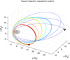 |
Fig. 1 Illustration of Cassini’s trajectory (about 25 orbits) during the SED storm from 27 November 2007 (marked by a triangle) until 15 July 2008 (marked by a square) in Saturn’s equatorial system. The trajectory is colored from blue (low inclination orbits) to red (high inclination orbits) to follow its temporal evolution. Saturn is schematically illustrated at the origin of the coordinate system with the z-axis along Saturn’s rotation axis, and the positive x-axis points toward the Sun in a plane formed by the rotation axis and the line from Saturn to the Sun. |
2.2 Cassini RPWS
The radio bursts of Saturn lightning were observed with the Cassini Radio and Plasma Wave Science (RPWS) instrument (Gurnett et al. 2004). In the frequency range of the SEDs the RPWS High Frequency Receiver (HFR) acted as a frequency sweeping receiver and swept from 325 kHz to ~ 16 MHz with an instantaneous bandwidth of 25 kHz within a few seconds. Different frequency step sizes, integration times, and antennas could be chosen resulting in many different observational modes. However, there were three prevalent modes with which the SEDs were observed (Fischer et al. 2011c), namely: (i) the survey mode, (ii) a fast polarimeter survey mode, and (iii) the so-called direction-finding (DF) mode (Cecconi & Zarka 2005). These modes are characterized by different duty cycles and detection efficiencies with respect to SEDs (see Appendix A). Shorter sweeping intervals and the usage of the more sensitive dipole in the survey mode typically led to about four to five times more SEDs in the survey mode (i) compared to the DF-mode (iii), where, in the latter mode, the RPWS monopole antennas are used. A description of how SEDs are extracted from RPWS data and the prescribed intensity thresholds are given in Fischer et al. (2006) and in Appendix B of this paper. Furthermore, the way SED polarization is measured is also described in more detail in this appendix.
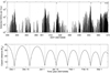 |
Fig. 2 Number of detected SEDs per hour in logarithmic scale as a function of time (in DOY 2007/2008, upper panel), and radial distance of Cassini as function of time (lower panel). This figure gives the first part of SED storm F from late November 2007 until 9/10 March 2008. The periapse times are marked by dotted vertical lines in both panels. The horizontal lines at the top indicate times when SED episodes lasted for a full Saturn rotation. |
2.3 Cassini ISS
The images shown in the next section were taken by the Wide Angle Camera (WAC) of the Cassini Imaging Science Subsystem (ISS, Porco et al. 2004). The WAC is a wide-angle refractor with 0.2 m focal length and a field of view of 3.5° and a CCD detector consisting of a 1024 square array of pixels. The storm clouds can be imaged with many filters that provide estimates of the cloud altitudes, for example, the narrow-band (5–20 nm wide) filters at the methane absorption bands MT1, MT2, and MT3 can probe different altitudes in the atmosphere. MT1 (central wavelength at 619 nm) and MT2 (727 nm) sense lower and intermediate cloud altitudes, respectively. Storm clouds were even seen at the strong methane absorption band MT3 at 889 nm. At this wavelength, MT3 senses the highest part of Saturn’s atmosphere, and the absorption optical depth of one (i.e., τ = 1) occurs at a pressure level of 0.33 bars (Dyudina et al. 2007). During SED storm F the cloud features were imaged by the ISS camera on seven different days, namely 6 December 2007, 4 March, 23 April, 19 May, 4 June, 18 June 2008, and 10 July 2008. The clouds were seen in day side images, typically observed with the clear filters (CL1, CL2) or the continuum band filters (CB1 at 619 nm, CB2 at 750 nm, CB3 at 938 nm).
2.4 Ground-based instrumentation
The Cassini optical observations are complemented by ground-based observations made by amateur astronomers. The latter provide more extended temporal coverage by monitoring the storm shape evolution and its longitudinal drift. The amateurs observed the storms on more than 70 days in the time interval from the beginning of December 2007 until the end of June 2008. The optical telescopes used by amateurs are mostly reflectors with an aperture from 15 to 40 cm (Delcroix & Fischer 2010). Many amateurs post their images at the website of the Planetary Virtual Observatory and Laboratory1 (Hueso et al. 2010) or the Association of Lunar and Planetary Observers (ALPO) of Japan2.
3 Observational records
3.1 Radio records
The SED storm before storm F had taken place in January and February 2006, and it was designated with the letter E (Fischer et al. 2007b). After storm E there was a long quiet period of about 21 months. During this time no SEDs and no prominent storm cloud features were observed by the Cassini instruments (Fischer et al. 2008). SED storm F described in this paper started in November 2007. We divide SED storm F into two different time intervals (Fischer et al. 2011c). Figure 2 shows the first interval of SED storm F from late November 2007 until early March 2008. The second interval of SED storm F displayed in Fig. 3 goes from early March 2008 until mid-July 2008. The first interval is characterized by a single storm cell. In the second interval SED storm F consists of two storm cells at the same latitude, but separated by ~ 25° in longitude.
The upper panels of Figs. 2 and 3 show the number of detected SEDs per hour as a function of time, and the lower panels show the spacecraft distance to Saturn. The vertical dotted lines in both panels of these figures indicate the times when the Cassini spacecraft was at periapses. The number of detected SEDs not only reflects the strength of the thunderstorm, but it is also a function of many observational parameters. The most influential parameter is the distance of the spacecraft, since the SED intensity falls off with distance squared, and so many low intensity SEDs are below the background level at large distances. Other observational parameters (see appendix) are the receiver mode, the attitude of the spacecraft, or the local time of the storm since the low-frequency cutoff of the SEDs is set by different peak electron densities in Saturn’s ionosphere on the day- and night side (Fischer et al. 2011c). From the vertical dotted lines in both panels of Figs. 2 and 3 one can see that peaks in SED numbers are mostly found around periapse passes.
Viewed from Cassini, SEDs from a single storm usually occur in episodes which start (stop) at the time when the storm enters (exits) the radio horizon. In general, the radio horizon of SEDs is not identical to the visible horizon of the storm seen from Cassini. It has been shown with previous SED storms, that the radio horizon usually extends beyond the visible horizon, which is called over-the-horizon (OTH) effect (Zarka et al. 2006; Fischer et al. 2007b). SED episodes are usually separated from one another by a quiet period of a few hours (absence of SED detections), since the presumably active storm on the other side of the planet (beyond the radio horizon) cannot be observed. In case of two storm cells with ~ 25° longitudinal separation (second part of SED storm F) the episodic on–off behavior is practically unchanged, only the SED activity will occur over an increased longitude range. In Figs. 2 and 3 the episodic behavior can hardly be seen due to the highly compressed time scale and the limited resolution of the figure (see e.g., Fig. 2 of Fischer et al. 2007b to discern episodic behavior). There are a few instances of time when the SEDs can be detected for more than a full Saturn rotation with no quiet period between consecutive episodes. Those times are marked with thick horizontal lines at the top of the upper panels in Figs. 2 and 3. One can see such lines three times after periapse passes in Fig. 2, and 14 times after periapse passes in Fig. 3. We believe that this is due to the over-the-horizon effect combined with a better visibility of the southern storm from higher southern spacecraft latitudes during periapse passes (see Sect. 5.3). However, in Fig. 2 there is one instance with continuous SED detections taking place when Cassini is more distant and located in the northern hemisphere. This is the case from 6–10 March when the RPWS instrument recorded no episodic gaps for nine consecutive Saturn rotations. This can only be explained by the presence of another storm, and we will discuss the reasons for the continuous SED detection in more detail in Sect. 5.4.
Figure 2 shows that the first part of storm F has several gaps in SED activity lasting for a few days or several Saturn rotations. For example, there is almost no SED activity for nearly five days right after periapsis of 27 January 2008. These gaps are due to internal variations of the strength of the thunderstorm, and such strong variations have been observed in previous storms (Fischer et al. 2006). We propose that some declines in SED activity during SED storm F are related to a splitting process of convective thunderstorm cells. This will be discussed in more detail in Sect. 5.6. Figure 3 shows the second part of SED storm F from early Marchuntil mid-July, where there are fewer gaps in SED activity. For example, there is one gap in SED activity from 11 to 14 March. There is strong evidence that there was a second active storm cell during the second part of the storm displayed in Fig. 3. This might be the reason for fewer gaps in SED activity, since it is less probable that two storm cells are inactive at the same time compared to just one inactive storm cell.
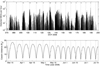 |
Fig. 3 Number of detected SEDs per hour as a function of time (in DOY 2008, upper panel), and distance of Cassini as function of time (lower panel). This figure gives the second part of SED storm F from 10 March until 15 July 2008. Similar to the previous figure, the periapse times are marked by dotted vertical lines in both panels, and the horizontal lines indicate times when SED episodes lasted for a full Saturn rotation. |
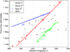 |
Fig. 4 Location of cloud features as a function of time as imaged by Cassini (diamonds) and ground-based amateur astronomers (dots). All longitudes in this figure and paper are western longitudes in degrees of Voyager SLS. The x-axis was inverted to have larger western longitudes on the left side. The y-axis goes from the start of storm F (27 November 2007) until its end (15 July 2008) with the start of the storm on the top. The different colors denote the storm cells F1, F2 and spot S3 as discussed in the text. |
3.2 Images
Storm systems with SED activity appear as bright white spots, most likely due to overshooting cloud tops as a result of a sudden increase in cloud vertical growth from updraft intensification. They are usually easy to identify on images of Saturn taken by the Cassini camera as well as on high quality images from ground-based telescopes made by amateurs (Porco et al. 2005; Delcroix & Fischer 2010). The prominent cloud features related to SED storm F were observed both by space- and ground-based instruments. The Cassini cameras imaged the clouds on seven different days mentioned in Sect. 2.3, and ground-based images show storm clouds starting from 1 December 2007 until 30 June 2008. The optical images showed that there is not only a single predominant cloud feature like in previous storms, but after mid-March 2008 there are at least two longitudinally separated storm cells.
Figure 4 shows the longitudinal location of prominent cloud features around 35°S planetocentric latitude from ground-based observations and Cassini ISS images as a function of time. The main cloud feature was centered around 36°S planetocentric latitude from the beginning to the end of the storm, and it drifted from ~ 270° to almost ~ 350° western longitude. All longitudes (and drift rates) in this paper are given in Voyager SLS (Desch & Kaiser 1981). The main feature F1 is marked as red line in Fig. 4, and a linear fit of all red points (from ground-based amateur as well as Cassini measurements) gives a drift of 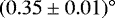 per Earth day. Taking the most prominent features from the Cassini ISS images from 6 December 2007 (DOY 340, at 275°) and 4 March 2008 (DOY 64, at302°) the drift is slightly smaller with 0.30° per day which is the value given by Fischer et al. (2011c) for the first part of SED storm F. We also note that the longitudinalas well as latitudinal extension of the storm is typically about 2°− 3°.
In mid-March 2008, a second bright cloud spot appeared around 38°S planetocentric latitude and around 280° longitude, roughly ~ 25° further east from the main drift line F1. This second storm marked withthe green drift line F2 was observed by many amateurs and Cassini, and it drifted at a rate of  per day. So due to the similar drift of cloud features F1 and F2 the longitudinal distance between both storm clouds was almost constant. Interestingly, this second storm cell F2 occurred in mid-March 2008 at a longitude around 280°, only 10° westward from where the first storm cell F1 emerged in late November 2007. The emergence of the second storm cell could be due to instabilities created by the first storm at the same longitude, or due to gravity waves from the first storm which have been observed to create additional cells in terrestrial thunderstorms (Balachandran 1980). This is similar to the later Great White Spot on Saturn, where additional thunderstorm cells developed in its eastward tail (Sayanagi et al. 2013).
Figure 4 also shows the drift of a third cloud feature called S3. This third cloud feature at 35°S planetocentric latitude existed from the end of January 2008 until the beginning of April 2008. Compared to F1 and F2, cloud feature S3 had a faster drift of 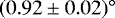 per day (blue line in Fig. 4). In the ground-based images S3 rather appeared as a faint spot in contrast to F1 and F2 which both appeared as bright white spots. We will discuss in Sect. 5.3 that the feature S3 probably did not show any SED activity, which is why we call it “spot” and not “storm”.
The red, green and blue lines in Fig. 4 describe the drifts of the clouds F1, F2 and S3, respectively. The linear dependence of their western longitudes θi (in degrees of Voyager SLS) as a function of time di (DOY 2007) is as follows:

Storm F1 lasted from 27 November 2007 until 15 July 2008. It was imaged for the first time on 1 December 2007 and for the last time on 30 June 2008, but in this case we set the limits from the beginning until the end of the SED activity. Storm F2 was observed optically from 14 March until 18 June 2008, although its SED activity probably last several days longer. The cloud feature S3 lasted from 27 January to 4 April 2008, as indicated by the limits for di in DOY 2007 in the equations above.
The drift of the storm cells around 0.35° per day corresponds to a westward wind speed of about 3.3 m s−1 with respectto the Voyager SLS rotation period. This is similar to previous SED storms of 2004–2006 around 35°S latitude, whose drift rates were in the range from 0.2–0.6° per day (Dyudina et al. 2007), corresponding to wind speeds of ~ 2–6 m/s. It is interesting to note that the zonal wind speed profile measured by Cassini ISS shows a westward peak velocity of (11.4 ± 3) m/s at that latitudes (García-Melendo et al. 2011). This difference could partly be due to vertical wind shear, which is a prerequisite for storm splitting as discussed in Sect. 5.6. Additionally, the peak of the westward jet is located at 34°S, whereas the storm cells rather tend to be centered around 36°S (Vasavada et al. 2006; Dyudina et al. 2007; Del Genio et al. 2007; Sromovsky et al. 2018), so there could be a small latitude difference. The drift speed of spot S3 with 0.92° per day corresponds to a speed of 8.9 m/s, which is within the error bars of the environmental wind given by García-Melendo et al. (2011). The drift speed of the head of the Great White Spot was even further away from the environmental winds: its westward drift rate of 2.8° per day corresponds to a wind speed of about 27 m/s (Sayanagi et al. 2013), and storms drifting with a different velocity than the environmental winds are suggestive of deeply rooted convection at the water cloud level (Sánchez-Lavega et al. 2011).
The amateur images of Saturn from February and March 2008 not only show the single storm cell F1, but there is also another cloud feature named spot S3 which is thought to have no SED activity. Figure 5 illustrates this with two images, one from 23 February and another one from 6 March. The latter even shows an extended storm cell F1, and it is interesting to compare it with the Cassini ISS image taken two days earlier. Figure 6 shows two Cassini images from 2008 with the storm clouds. The left image taken on 4 March shows the single bright storm F1, and we have also indicated the features A, B, and C corresponding to the right image from Fig. 5. The largest cloud feature A corresponds to the storm cloud F1. The left Cassini image of Fig. 6 actually shows that features B and C are dark ovals. Feature B, which looks like a westward extension of A (F1) in the ground-based image, turns out to be a dark oval being close to storm F1. Feature C corresponding to spot S3 also turns out to be a large dark oval in the high-resolution Cassini image. The different appearance is mostly due to the usage of different filters in the ground-based image (green filter) versus the Cassini image (continuum band filter CB3 around 938 nm). There is also a Cassini image from 4 March taken with a green filter (not shown), which shows faint white spots as features B and C. Furthermore, some dark vortices are sometimes accompanied by bright features as well. The notion that spot S3 is actually a large dark oval is also supported by an image taken with Cassini VIMS (Visual and Infrared Mapping Spectrometer) on 9 February 2008. Figure 5 inSromovsky et al. (2018) shows this dark oval around 300° western longitude (60° eastern longitude), about 8° in longitudewestward of the bright thunderstorm. These longitudes are consistent with the longitudes of S3 and F1 shown in Fig. 4 for the first half of February 2008. The reason why only this dark oval (and not numerous other ones) was seen as faint spotin the ground-based images is probably its exceptionally large size. There are no other Cassini ISS images of spot S3 except those of 4 March.
The right image taken on 18 June shows a pair of bright white features (F1 on the left, F2 on the right) at the same latitude, separated by about ~33° in longitude. For the observation of 18 June the observed storm cloud longitudes are somewhat off from the linear fits of Eqs. (1) and (2). Using the fitted lines the longitudinal difference between storms F1 and F2 varies only from ~26.7° to ~27.5°. Again one can see some more dark ovals which are located at the same latitude as the bright spots in the well-known storm alley at ~35° south. For example, one can easily identify 3 dark spots between the two white spots in the 18 June image of Fig. 6 (right panel). The relation between the dark ovals and the convective storms will be further discussed in Sect. 5.5 in comparison with previous works (Dyudina et al. 2007; Baines et al. 2009; Sromovsky et al. 2018). It is likely that the SED activity of storm cell F2 started exactly on 14 March 2008, since this is the first day when we have a clear evidence of it in ground-based images3. Furthermore, there was very little SED activity from 10 March noon until 14 March at 06:00 SCET (see Fig. 3), and SED rates started to rise again exactly on 14 March. The exact end of SED activity in storm cell F2 can not be determined since it is impossible to distinguish it from SEDs from F1.
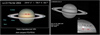 |
Fig. 5 Amateur images of Saturn with south pointing upward from February and March 2008. Left panel: RGB image of Saturn taken by Jean-Jacques Poupeau on 23 February 2008, 23:47 UT. The prominent cloud feature close to the central meridian is the storm cell F1. The faint cloud feature about 20° westward of F1 is marked with red lines, and this is spot S3 as discussed in the text. Right panel: Saturn image in green filter taken by Maximo Suarez on 6 March 2008, 23:20 UT. The magnified inset panel shows four features named A, B, C, and D, where the latter is questionable. Feature A corresponds to storm cell F1 with feature B being a westward extension of A. Feature C corresponds to spot S3. |
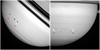 |
Fig. 6 Cassini ISS images from 4 March 2008 (left panel), and 18 June 2008 (right panel). The left image shows mainly one bright storm cloud, whereas there are two bright storms in the right image. In the 4 March image the bright storm F1 is located at 302° western longitude. We have marked the features A, B, and C corresponding to the features shown in the right panel of Fig. 5, that were imaged by M. Suarez two days later. This shows that spot S3 is actually a large dark oval. The 18 June image shows two bright spots at 310.3° (F2) and at 343.4° (F1) western longitude, with the older storm cell F1 further west (left) than the younger storm cell F2. All spots are located around ~35° south planetocentric latitude. The left image (file name W00043078.jpg) was taken with filters CB3 and CL2, and the right image (file name W00046585.jpg) was taken with filters CB3 and IRP0 (Images by NASA/JPL/SSI). |
4 Statistical analysis
In this section we analyze the SED intensities, polarization, burst rates, and the durations of the SED episodes for the complete storm. Using the detection criteria described in Fischer et al. (2006) and in the appendix, 277 046 SEDs were detected during storm F. The SEDs were made up of more than half a million SED pixels (500 492 single time–frequency measurements). One SED is produced by a single lightning event. Since its duration can be longer than the receiver integration time (typically 35 ms) at one frequency, several measurements at successive frequency channels (“SED pixels”) can be made during one SED. Using the numbers above, an average SED consists of 1.8 SED pixels. About 68.5% of the SED pixels were detected in the survey mode, ~23.0% in the fast polarimeter mode, and ~8.5% in the DF-mode. The number of SEDs detected during SED storm F is a factor of about 12 higher than all SEDs detected by both Voyagers (~ 23 000 SEDs), and a factor of 5–6 higher than all SEDs detected by Cassini during the previous shorter storms (~ 49 000 SEDs). Hence, we employ a statistical analysis and compare the results with previous storms.
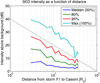 |
Fig. 7 Intensities of SED storm F pixels as a function of distance between storm F1 and Cassini. The data was divided in 18 distance intervals with a bin size of 2 RS, centered at the values of 3, 5, 7,... 37 RS. For each interval we calculated the median intensity value (50% percentile, blue curve), the 80% percentile (green curve), the 95% percentile (red curve), and the maximum (100% percentile, cyan curve). The gray line represents an inverse-square law ( |

4.1 SED intensities
Since the geometrical dimensions of the SED source are much smaller than the distance to the observer, the SED intensity is an inverse-square function of distance. Using such an approach, Zarka (1985) obtained a reasonable agreement between model and measurements of the variation of SED maximum intensity as a function of time during the Voyager 1 flyby. Previous Cassini SED measurements with sufficient SED rates were made only during parts of one orbit with small variations in distance. For storm F the distance variation was more than one order of magnitude (about 3 RS to about 37 RS). Figure 7 shows a statistical analysis of the SED intensities as a function of distance. We binned all SEDs as a function of their distance to the planet in 18 bins with a bin size of 2 RS (centered at values from 3 RS to 37 RS). For each binwe calculated the intensities of the percentiles of 100, 95, 80, and 50%. The 50% percentile is the median value, and half of the SED pixels in that bin are smaller than the median intensity. The intensities of the 100% percentile represents the maximum, and SEDs are detected from the detection threshold (see appendix) up to the maximum intensity. The cyan curve as the maximum SED intensity in Fig. 7 follows the inverse-square law relatively well (gray line). The same holds for the red curve representing the 95% percentile. The small variations in the curves are probably due to the internal variation of the storm’s intensity or due to different ionospheric conditions. There are probably no beaming effects since SEDs are thought to radiate isotropically (Zarka 1985), but absorption generally depends on the ionospheric electron density which is varying with local time. The most intense SED pixel was detected on 18 May 2008 at 02:01 SCET (spacecraft event time) with an intensity of 39.5 dB above the background. The mean intensity of all storm F SED pixels is 6.0 dB, and the median intensity is 3.9 dB. After the model of Dulk et al. (2001) the galactic background has a relatively constant flux density of ~ 10−19 W m−2 Hz−1 in the frequency range of the SEDs from 2 to 16 MHz (see Fig. 1 in Zarka et al. 2004). This means that the flux densities of the detected SED pixels range over almost four orders of magnitude from ~ 10−19 to ~ 10−15 W m−2 Hz−1. The antenna resonance around 7–8 MHz is also in the SED frequency range, but it enhances both the background and the signal.
The distribution of SED intensities approximates an exponential law as can be seen in Fig. 8. Similar distributions for single SED episodes have already been shown in Fischer et al. (2007b). The small plateau in the first one or two bins close to the intensity threshold for the distribution of intensities over all episodes is due to the detection algorithm (see appendix) in combination with the varying distance of the spacecraft. In Fig. 8 we also show the relative similarity of the intensity distribution of all SED pixels (in gray) to those from the single episode (in black) of 10 May 2008 before noon, when Cassini was very close to Saturn. We also note that for such a closest approach episode, where SED intensities typically extend over more than three orders of magnitude (see Fig. 7), the shape of the distribution is similar to an exponential decay. Only the SEDs above the intensity threshold are detected, and these SEDs lie on the tail of a distribution whose shape can also be modeled with a generalized extreme value distribution (Pagaran & Fischer 2014). With such a model fit it could be possible to roughly estimate the number of SEDs below the detection threshold. Here we only use a two-term exponential model to fit the distribution of all SED intensities. The dashed fitted curve in Fig. 8 is given by
 (4)
(4)
with I as the intensity in dB above background and N as the number of SED pixels. The first term approximates the intensities above ~ 5 dB, whereas the second term mainly fits the intensities below ~5 dB. The first bin was not included in the fit due to the close threshold level.
4.2 SED polarization
The polarization of SED radio waves is an important property with which the hemisphere and the emission mode of the SED source can most likely be determined. The methodology to determine the SED polarization from RPWS measurements is described in Fischer et al. (2007a) and shortly summarized in Appendix B of this paper. Fischer et al. (2007a) found right-hand polarized SEDs below 2 MHz from a southern hemisphere source and suggested that the polarization sense is related tothe direction of the magnetic field in the two hemispheres relative to the radio wave propagation vector. They suggested that the ordinary mode is dominant (the extraordinary mode is more attenuated) leading to right-handed SED polarization from southern hemisphere sources since the radio wave propagation vector is opposite to the magnetic field vector there. Consequently, SEDs from the northern hemisphere should be left-hand polarized, which was the case for the SEDs from the first giant thunderstorm of 2010/2011 observed in the northern hemisphere by Cassini (Fischer et al. 2011b). Fischer et al. (2007a) measured the SED polarization of SED storm E from January and February 2006, and since then several other SED storms have occurred at a latitude of 35° in the southern hemisphere, whose polarization analyses are yet to be performed.
The vast majority of SEDs from storm F below 2 MHz exhibit a right-handed circular polarizationsimilar to storm E. The polarization is described by the Stokes parameters q, u, and v. The mediancircular polarization of more than 6000 SED pixels below 2 MHz from storm F is  , the median linear polarization is
  , and the median total polarization is
  . Left-handed polarization was found for only ~2.6% of the SED pixels. In principle, no SED should have a total polarization of d > 1, but about 5.1% of the SED pixels show a total polarization larger than one. This is mostly due to errors in the polarization measurement, which are typically around 15%. This confirms the results and conclusions of Fischer et al. (2007a).
We note that we also tried to perform a direction-finding analysis of storm F SED radio waves, since RPWS has such a capability, and since it would be interesting to see if in this way the two storm cells F1 and F2 could be discerned. However, this attempt was not successful. We used almost the same data as for the polarization measurements (i.e., below 2 MHz, see appendix), but limited them to a Cassini distance of less than 12 Saturn radii. From these ~ 5500 SED pixels, about 60% were retrieved in a 2-antenna mode, and about 40% with the 3-antenna mode. For the 2-antenna mode the direction-finding has to be done with the assumption of pure circular polarization (Stokes parameters q = 0 and u = 0), and this is a crude assumption since the median linear polarization of SEDs was found to be  (see above). As a consequence only 12% of the 2-antenna SED pixels had an incoming radio wave vector that originated from the planet Saturn. Surprisingly, this rate was even smaller (only 1.5%) for the the 3-antenna SED pixels for which no assumption about the linear polarization has to be made. The reason for this failure is most likely due to the fact that the RPWS 3-antenna direction-finding mode uses two consecutive 2-antenna measurements separated by 10–160 ms in time depending on the receiver mode (Gurnett et al. 2004, Vogl et al. 2004). Since SEDs are short and bursty signals, their properties might change within this delay time of several tens of milliseconds, thereby corrupting the 3-antenna direction-finding measurement.
 |
Fig. 8 Distribution of SED pixel intensities of storm F with a bin size of 0.4 dB. The gray bars represent all SED pixels, and the black bars show the distribution of pixels from a single SED episode, the closest approach episode of 10 May 2008 before noon. For a better visibility the black bars of the single episode are magnified by a factor of 10 with respect to the scale on the ordinate. The dashed fitted curve is given by the two-term exponential model of Eq. (4). |
4.3 SED burst rates and durations
The SED burst rates highly depend on the distance of the spacecraft to Saturn and are typically ~ 102 h−1 at average distances and reach ~ 103 h−1 at periapse as can be seen in Figs. 2 and 3. The highest rate of 3872 h−1 (about 1 SED per second) was measured on 20 February 2008 from 13:00 to 14:00 SCET. With 277 046 SED detections (not SED pixels) during 2578 h one arrives at an average rate of 107 h−1 (~ 1.8 SEDs min−1). The 2578 h is the sum of all episode durations during the 231.38 days (5553 h) of SED storm F from 27 November 2007 until 15 July 2008, that is SEDs were detected for slightly less than half of this time only when the storm was on the side of Saturn facing Cassini.
All the burst rates given so far are as detected, which means they do not account for the duty cycle of the instrument. The duty cycle gives the percentage of time the receiver dwells at SED frequencies, which depends on the mode of the instrument. For the mostly used survey mode the duty cycle is 32%, and a combined duty cycle taking into account the number of detected SEDs in each receiver mode is 34.4% (see appendix). The detected average rate of 107 h−1 then corresponds to a so-called extrapolated or “true” rate of ~ 311 h−1 (~ 5.2 SEDs min−1) for SED storm F. This rate is similar to the true rate of 367 h−1 of SED storm E (Fischer et al. 2007b). The SED peak detection rate of 3872 h−1 during SED storm F was measured in the fast polarimeter mode with a duty cycle of 47% (see appendix), hence, the true peak rate would be 8238 h−1 (or ~2.3 SEDs per second). However, we note that these extrapolated values do not reflect the absolute SED rate of the storm. An increasing number of SEDs drops below the galactic background level for an increasing spacecraft distance, and we only see the tail of the intensity distribution (see Sect. 4.1). Other factors influencing the SED detectability are the spacecraft-antenna attitude, the different sensitivities of RPWS dipole and monopole, and the local time of the source influencing the SED ionospheric absorption and cutoff frequency. In a future paper we will try to get a better estimate for the true SED rate by taking all these points into account.
The SED burst durations follow an exponential distribution given by n ∝exp(−t∕t0). This means that the number of SEDs n is exponentially decreasing with increasing burst duration t. The distribution is characterized by the so-called e-folding time t0 with typical values from ~35 to ~50 ms (Fischer et al. 2008). For example, the SEDs from the previous SED storm E recorded in the survey mode had an e-folding time of (49 ± 3) ms (Fischer et al. 2007b). For SED storm F we found an e-folding time of (49 ± 1) ms for the SED recorded in the survey mode (above 1825 kHz), and an e-folding time of (46 ± 1) ms for the SEDs in the fast survey mode. The mean SED duration is (66 ± 45) ms for the SEDs above 1825 kHz in the survey mode, and it is (54 ± 42) ms for the SEDs in the fast survey mode. The combined value for the mean SED duration in these two modes would be (63 ± 45) ms. The SEDs measured in the direction-finding mode (and in the survey mode below 1825 kHz) have such long integration times (> 80 ms) that they would skew the result toward longer times, and so we excluded them here.
4.4 SED episode durations
SEDs are usually organized in episodes, lasting typically half a Saturn rotation. Saturn’s atmospheric storm features have a higher angular velocity than the observer Cassini around Saturn leading to a cessation of SEDs when the source is beyond the radio horizon. Figure 9 shows the distribution of episode durations of all 439 SED storm F episodes plus so-called pre- and post-episodes that will be explained in the next subsection.
The duration of an SED episode depends on several factors. Many SED episodes typically last somewhat longer than half a Saturn rotation (due to the over-the-horizon effect), and in Fig. 9 one can see a peak around an episode duration of six hours. This is followed by a sharp decline toward longer episode durations up to ten hours. The longer durations should be due to the addition of the second storm cell after March 2008 (see Figs. 4 and 6) and an extension of the radio horizon when Cassini is at middle to high southern latitudes. There is even a small hump with episode durations from 10 to 13.5 h with some of these lasting even longer than the Saturn system III period of 10.6567 h (Desch & Kaiser 1981). These are the closest approach (periapsis) episodes where Cassini has a high angular velocity (in the same sense as the rotation of Saturn) andcan follow the SED storms for some time. This effect has already been modeled by Zarka (1985) for the Voyager flybys of Saturn during which the SEDs were discovered. At large radial distances from Saturn a spacecraft can be regarded as an almost stationary observer where the subspacecraft western longitude changes by 360°∕10.66 h ≈ 34° h−1. During periapse passes with closest approach radial distances around 4 RS this rate went down below 20° h−1 for Cassini, thereby prolonging the time of visibility of an atmospheric feature. In the cases where one SED episode follows immediatelyafter the other (i.e., continuous SED detections without gap between episodes) it is sometimes difficult to tell when one episode ends and the next one begins. One way to do this is to place the boundary at the minimum of the SED rate profile. This was difficult during the interval 6–10 March 2008 when the SED activity and detection continued for nine consecutive Saturn rotations without interruption. In that case we arbitrarily placed the boundary between episodes at roughly the same subspacecraft western longitudes. We define one SED episode as the SED activity related to one Saturn rotation as viewed from the spacecraft. This means that we understand one Saturn rotation as the somewhat variable time (longer at periapsis!) during which the subspacecraft longitude completes 360°. So the continuous SED detection from 6–10 March 2008 (DOY 066–070) consists of nine SED episodes (cf. episodes F175–F183 of Table C.1 in the supplementary material) and not just a single one. In Figs. 2 and 3 we have indicated the times when SED episodes lasted longer than one Saturn rotation which, with the exception of 6–10 March 2008, always happened at the periapse passes. The episodes from those times make up the small hump from 10 to 13.5 h in Fig. 9.
The mean duration of the 439 regular episodes is 5.63 h. The longest SED episode lasted 13.36 h, and that was the periapsis episode of 16 June 2008 centered around noon (cf. episode F382 of Table C.1 available at CDS). This table enlists the most important characteristics of the 439 SED episodes. The table gives the episode name, center, start and stop times of each episode, the number of detected SEDs and SED pixels, the mean distance of Cassini, the subspacecraft western longitude at the episode center, and the subspacecraft western longitude range of the episode from the beginning to its end. The table also shows the 83 pre- and post-episodes. Pre-episodes are indicated by an additional letter “a” at the episode’s name, and for post-episodes the additional letter “b” is used. Figure 9 shows episode durations that are shorter than half a Saturn rotation. Some episodes are simply shorter due to low SED rates. But, the peak in the first bins is due to the existence of what we call pre- and post-episodes. Their characteristics are described in more detail in the next section.
 |
Fig. 9 Distribution of SED storm F episode durations in half hour bins in a stacked histogram. The distribution contains 522 values, which includes 439 regular episodes, 49 pre-episodes, and 34 post-episodes. |
 |
Fig. 10 Sample episodes with pre- and post-episodes. Left panel: storm episode F298 with a pre-episode. Right panel: episode F036 with a post-episode. We show the extracted SEDs displayed versus time (in hours of SCET, spacecraft event time) and frequency. The frequency range (with linear scale from 1.8 to 16.2 MHz) in the left and right panels are exactly the same. In the left panel nine hours are displayed, and in the right panel it is seven hours. The colors indicate the SED pixel intensities in dB above background. |
5 Discussion
This discussion section contains descriptions and investigations of noteworthy phenomena that occurred during SED storm F. In the first subsection the new phenomenon of SED pre- and post-episodes is described. In the next subsection the course of the SED storm F is illustrated with a plot of the subspacecraft western longitude ranges of SED episodes as a function of time. Here we will discuss if the second and third cloud features F2 and S3 showed electrical activity or not. This is followed by a discussion of the over-the-horizon effect in the third subsection. Next we will try to explain the continuous SED detection from 6–10 March 2008. In the fifth subsection we discuss the presence of dark ovals that are most likely not electrically active but are seen in images throughout the lifetime of SED storm F. In the sixth and final subsection we consider the dynamics of Saturn’s thunderstorm and suggest that some decreases of SED activity might be related to splitting thunderstorm cells.
5.1 Description of SED pre- and post-episodes
Figure 10 shows a typical pre-episode in the left panel, and a typical post-episode in the right panel, displayed as extracted SEDs versus time and frequency. The left panel shows a pre-episode with a duration of about two hours (from 14 to 16 h SCET), which is separated by at least one hour from the main episode, which starts after 17 h SCET. Its most striking characteristic is its limited frequency range from ~ 2−6 MHz. Similarly, the right panel shows a so-called post-episode around 17 h SCET, which appears to be separated from the main episode and starts roughly one hour after the main episode ended. Its frequency range is even more limited, from ~ 2−4 MHz. In summary, the limited frequency range and the separation from the main episode are the two defining characteristics of pre- and post-episodes.
Since the lightning discharges are stochastic and can occur at any time, the frequency-sweeping receiver can dwell at any frequency during the time of the discharge. As a consequence, in the general case of straight-line propagation from the source to Cassini, SEDs should be equally distributed at frequencies above the ionospheric cutoff frequency. Since this is not the case for pre- and post-episodes, it is likely that they arise from an ionospheric propagation effect of SEDs from the main storm cloud, and not from another storm cloud which is within the visible horizon of the spacecraft.
For both panels of Fig. 10 one can see that the temporal difference between the center of the respective main episode and the pre- or post-episode is around four hours. This translates to a western longitude difference of ~ 120°, which means that they are observed at a time when the storm cloud is beyond the visible horizon. Hence, we suggest that the existence of pre- and post-episodes is a consequence of the over-the-horizon effect, which will be described in more detail in Sect. 5.3. It has already been observed for previous SED storms that the over-the-horizon effect is alsofrequency dependent, and frequencies above 10 MHz are almost never observed beyond the visible horizon (Zarka et al. 2006; Fischer et al. 2007b; Gautier et al. 2013). The pre- and post-episodes show an even more restricted frequency range, and they are a new phenomenon which occurred first with SED storm F. There are a few cases of SED episodes with three parts, that is a main episode which is accompanied by a pre-episode and a post-episode, but usually there is either a pre-episode or a post-episode. Figure 9 shows that the absolute majority of all 49 pre-episodes and 34 post-episodes are shorter than one hour, and almost all of them are shorter than 2.5 h. The mean duration of the 83 pre- and post-episodes is 0.97 h. According to our definition, a short pre- or post-episodeis not regarded as a full episode, since only together with its main episode it represents the SED activity of one Saturn rotation viewed from the spacecraft. Nevertheless, we show the statistics of the pre- and post-episodes in Fig. 9 since they are a new and interesting phenomenon. The duration of the main episodes of Fig. 9 is determined without taking the durations of the pre- or post-episodes into account.
Figure 11 shows the position of Cassini in local time and kronocentric latitude during the times when pre-episodes (magenta stars) or post-episodes (cyan stars) were recorded. It can be clearly seen that pre- and post-episodes were preferentially observed from ± 3 h around localnoon, that is when the storm cloud was either located around local dawn or local dusk. Both pre- and post-episodes also rather tended to occur when Cassini was at northern latitudes. The black dots show which regions of local time and latitude were sampled by Cassini during SED storm F. Cassini was mostly on the morning side in the southern hemisphere and on the afternoon side in the northern hemisphere. The equatorial plane was crossed at almost fixed local times, around 23 LT at periapsis and around 11 LT at apoapsis. The Cassini latitude was increasing with time, see also Fig. 1.
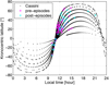 |
Fig. 11 Local time and kronocentric latitude of Cassini during the recording of pre-episodes (magenta stars) and post-episodes (cyan stars). The black dots show the position of Cassini in local time and latitude from 27 November 2007 until 15 July 2008 with a resolution of one dot per hour. |
5.2 Distribution of episodes in subspacecraft western longitude
The course of SED storm F can be illustrated with the following Figs. 12 and 13 which plot the subspacecraft western longitude ranges of SED episodes as a function of time. Due to the long duration of SED storm F, we have subdivided the plot of SED western longitude ranges versus time into two figures. Figure 12 extends from the beginning of the storm in the end of November 2007 until mid-March 2008, and Fig. 13 shows the longitudinal range in the same format from mid-March to the end of the storm in mid-July 2008. The western longitude ranges of the SED episodes are displayed as almost vertical black lines in different line styles (solid, dashed, dotted) depending on the number of SEDs of the respective episode (≥ 200, 20–200, < 20). Each line is drawn from the time/western longitude coordinate when the SED episode starts until it ends, with the end point always at a larger western longitude than the start point (i.e., we add 360° for end points with western longitudes smaller than at start points). This leads to a clearer arrangement compared to a plot with a strict western longitude range from 0° to only 360°, and it can be seen in Figs. 12 and 13 that a y-axis range over 1.5 rotations (0°−540°) is sufficient to display all SED storm F episodes in such a way.
For each SED episode there is a red asterisk which is located roughly in the middle of each episode. It marks the mean western longitude at the so-called episode center time, which is the mean time of all SEDs from the respective episode. Similarly, the mean western longitude is the mean longitude of all SEDs from one episode. In Fig. 12 these red asterisks gather around the almost horizontal solid red line, which displays the west longitude of the visible storm cloud F1 as a function of time. The solid red line has a slope of ~0.35° per day as stated in Eq. (1). A linear fit of the center times of all SED episodes with more than 20 SEDs versus western longitude over the time of Fig. 12 (start of storm until 15 March 2008; and excluding episodes with a mean western longitude smaller than 200° and larger than 360°) gives a line with a slope of 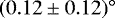 per day, which means it is somewhat smaller than the drift of the visible storm cloud. However, another linear fit of the same parameters over the time of Fig. 13 (15 March 2008 until end of storm) gives a line with a slope of
  /day with the intercept
  . In this case the slope of the fitted line is close to the ~0.35° per day for the visible storm cell F1. The second storm cell F2 has practically the same slope as storm cell F1, but its intercept of 124° (see Eq. (2)) is 31° smaller than the intercept of F1. The intercept of F2 is relatively close to the intercept of the fitted line, which means that our linear fit is close to the position of storm cell F2. This can be seen in Fig. 13, where the red asterisks rather gather around the dashed red line describing the western longitude drift of the second storm cell F2 than around the solid red line of storm cell F1. This is a clear indication that (besides the initial storm cell F1) the second storm cloud F2, which emerged in mid-March 2008, is also a thunderstorm emitting SEDs. Other arguments supporting this notion is the large optical brightness of the storm cell F2 as it can be seen in the right panel of Fig. 6, and the increased longitude range of SED episodes in the second half of the storm. The average longitude range of all SED episodes (pre- and post-episodes excluded) of Fig. 12 from the beginning of the storm until mid-March 2008 is 165°, and the average longitude range of all SED episodes of Fig. 13 from mid-March 2008 until the end of the storm is 188°. The difference of 23° is close to the longitudinal separation of the visible storm clouds F1 and F2 of 27°, suggesting that both storm clouds emit SEDs in the second half of SED storm F.
The western longitude of the third visible cloud S3 is indicated in Figs. 12 and 13 by a barely visible red dotted line that starts in the end of January 2008 in Fig. 12 and ends in early April 2008 in Fig. 13. During the course of the time it drifts to larger western longitudes with a rate of ~ 0.92° per day (see Eq. (3)). In the days after mid-March it has drifted to a western longitude of ~ 340°. If the spot S3 would emit SEDs at that time, they should be detectable in a western longitude range up to ~ 420−430°, but there are barely any SEDs beyond 360° from 15 to 20 March, for example. This suggests that the spot S3 is not a thunderstorm and does not emit SEDs, at least in the second half of SED storm F displayed in Fig. 13. We cannot judge the SED activity of spot S3 with this method before that time (February to mid-March 2008) since it is to close to the main storm cloud F1. However, the appearance of spot S3 as dark oval in the Cassini images suggests that it did not emit any SEDs.
A good way to characterize the visibility of the storm cloud from the observer Cassini is the emission angle α. It is defined as the angle between the local zenith at the location of SED storm F1 and the vector from the SED storm to Cassini. We calculated the angle α as a function of time, taking the oblateness of Saturn into account. The green dots mark the times and subspacecraft western longitudes when the emission angle α is 90° (storm cloud exactly at the visible horizon seen from Cassini), and the blue dots indicate the times and western longitudes for α =135° (storm cloud beyond the visible horizon by 45°). It is interesting to note that the green and blue dots in Figs. 12 and 13do not form straight lines, but can also show variations from one Saturn rotation to the next. For example, the minimum longitude range between two green dots at the same Saturn rotation is just ~ 4° (22 March), and the maximum longitude range is up to ~252° (30 June) with an average longitude range of the visible horizon of 151° (from where the storm is visible by Cassini). These variations are increasing from one Cassini orbit to the next, and they are related to the increasing inclination of the spacecraft’s orbit. The reason why the average longitude range of the visible horizon is by almost 30° smaller than half a Saturnrotation (180°) is due to thefact that during SED storm F Cassini spent 77% of the time in the northern hemisphere from where a storm located at a latitude of 35° south is observed more rarely. Figure 12 shows that for a spacecraft with a low latitude (first two to threeorbits during SED storm F in December 2007) the longitude range of the visible horizon is around 180° and the α = 90° boundary does not vary that much. Indeed, for a spacecraft in the equatorial plane it would be possible to approximate the α =90° boundaries by straight lines shifted by ± 90° from the western longitude position of the storm cloud. This approximation was applied by Fischer et al. (2007b) in their Fig. 7 for SED storm E since the Cassini latitude was always within ± 1° of the equatorial plane and Cassini’s distance was mostly beyond 20 Saturn radii. The variation of the longitude range of the visible horizon depending on Cassini’s latitude (neglecting Cassini’s distance which is always larger than 2.5 Saturn radii during SED storm F) can be understood in the following way. The visibility of the SED storm at 35° south is worst (minimum longitude range between green points in Figs. 12 and 13) when Cassini reaches its highest northern latitude (around 17 h Cassini LT), which usually happens a few hours before periapsis. Then the northern latitude decreases quickly, the ring plane is crossed around periapsis (around 23 LT), and a few hours later Cassini reaches its highest southern latitude (around 5 LT, see Fig. 11 or Fig. 1). At such high southern latitudes the visibility of the southern SED storm reaches its maximum (maximum longitude range between green points), and the change from minimum to maximum storm visibility happens within less than one day. The boundaries of α = 135° (blue dots in Figs. 12 and 13) show a similar variation due to the same reason related to the latitude of Cassini. We also note that the boundaries of α = 90° and α = 135° are drawn in Figs. 12 and 13 only for storm F1, and not for storm F2 which also shows SED activity. We refrained from drawing the boundaries for storm F2 since the plots would be too confusing with so many lines. The shapes of the these boundaries for storm F2 would be similar to storm F1. One can imagine them as the boundaries of storm F1 shifted by 27° to smaller western longitudes, since storm F2 is located 27° further east than storm F1 at the same latitude.
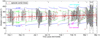 |
Fig. 12 Subspacecraft western longitude ranges of SED episodes from the end of November 2007 until mid-March 2008. The western longitude ranges are displayed as almost vertical black lines. These lines are dotted for SED episodes with less than 20 SEDs, dashed for episodes with more than 20 but less than 200 SEDs, and solid for episodes with greater than or equal to 200 SEDs. For each episode the red asterisk marks the western longitude at the center time of the respective episode (i.e., mean time of all SEDs from this episode). The western longitude ranges of pre-episodes are colored in magenta, and the ranges of post-episodes are colored in cyan. The almost horizontal red lines indicate the western longitudes of the storm cells F1 (red solid line), F2 (red dashed line), and S3 (red dottedline), respectively. Similar to Fig. 2, the black horizontal lines on top indicate times when SED episodes lasted for a full Saturn rotation, which means that the western longitude range goes up to 360° for such episodes. Additionally, the interval of continuous SED detections from 6–10 March is indicated by black vertical dot-dashed lines. The green dots mark the times and subspacecraft western longitudes when the emission angle α is 90°, and the blue dots indicate the times and western longitudes for α = 135°. The angle α is defined as the angle between the local zenith at the location of SED storm F1 and the vector from the SED storm to Cassini. More detailed explanations can be found in the text. |
 |
Fig. 13 Subspacecraft western longitude ranges of SED episodes from mid-March until mid-July 2008. The figure has the same formatas the previous Fig. 12. |
5.3 Over-the-horizon effect
The over-the-horizon (OTH) effect is the effect that SEDs can be detected by Cassini even when the SED source is beyond the visible horizon as seen from the spacecraft. This means that there is a radio horizon extending beyond the visible horizon, and the effect was described by Zarka et al. (2006), Fischer et al. (2007b), and Dyudina et al. (2007). A potential explanation was first offered by Zarka et al. (2006), who proposed that it is due to a temporary trapping of SED radio waves below Saturn’s ionosphere before they are released. A quantitative modeling with ray-tracing was successfully performed by Gautier (2013), Gautier et al. (2011, 2013). They used an ARTEMIS-P code, a ray tracing code in magnetoionic plasma, and showed that the OTH effect is frequency dependent.
The over-the-horizon effect can also be illustrated with plots like Figs. 12 and 13. As already mentioned, the green dots in Figs. 12 and 13 mark the times and western longitudes when the emission angle α equals 90°. This means that at α = 90° the storm cloud is exactly at the visible horizon as seen from Cassini. The western longitude region between the green points (e.g., from about 180° to 360° at the end of November 2007, see Fig. 12) marks the times and western longitudes when the SED storm is within the visible horizon as seen from Cassini, where α < 90°. It is obvious(see Figs. 12 and 13) that most SEDs are detected when the thunderstorm can be seen from Cassini, and the radio waves propagate in a straight line to the RPWS antennas on Cassini. However, there are also many SED episode longitude ranges (vertical black lines) that extend beyond the limit of α =90°, and all SEDs detected outside this region experience the over-the-horizon effect, which means that the radio waves can reach Cassini although the storm cloud is not within the visible horizon anymore. In Figs. 12 and 13 we have also used blue dots to indicate the times and western longitudes when the emission angle α equals 135°. This value was taken because previous observations (Zarka et al. 2006; Fischer et al. 2007b) have shown that the over-the-horizon effect typically extends 45° beyond the horizon. Indeed, most SED episode ranges are limited by the blue dots in Figs. 12and 13, and only a few extend beyond that. The so-called pre- and post-episodes, marked by magenta and cyan color in Figs. 12 and 13, are typically located around the α = 135° boundary or partly beyond it. This substantiates our claim that the pre- and post-episodes are manifestations of an extreme over-the-horizon effect.
It can clearly be seen in Figs. 12 and 13 that the longitudinal extension of SED episodes (length of vertical black lines) mostly reaches a maximum shortly after periapsis when the storm’s visibility also has its maximum. Additionally, some of these SED episodes have longitudinal extensions up to 360°, albeit the fact that the maximum longitude range of the visible horizon for SED storm F is only ~ 252°. In this case the SED storm must be within the radio horizon (which is larger than the visible horizon) for a full Saturn rotation, even when the storm cloud is on the opposite side of the planet as viewed from the spacecraft (i.e., shifted by 12 h in local time). We have indicated the SED episodes lasting for a full Saturn rotation in Figs. 12 and 13 by horizontal black lines at the top. With a single exception (6–10 March) these horizontal black lines only occur right after Cassini periapsis, when the storm’s visibility has its maximum. Very often there is not just a single SED episode with a longitudinal extension of 360°, but a few of them with one following the other. In these cases we have no obvious gaps between consecutive episodes for a few Saturn rotations. Here we usually set the boundary between one SED episode and the next around the minimum of the SED rate, since we define one SED episode as related to just one Saturn rotation and not several Saturn rotations. A detailed inspection of Figs. 12 and 13 shows that the SED episodes with longitudinal extensions up to 360° right after Cassini periapse passes can be explained by the over-the-horizon effect. After most periapse passes there are actually no blue points denoting the α = 135° boundary for some time. This means that we have α < 135° for a few Saturn rotations, and during this time the storm cloud is within the radio horizon of 45° beyond the visible horizon. The geometry is such that with Cassini at high southern latitudes and the storm cloud at 35° south, we have an emission angle α < 135°. It would be interesting to know how the radio waves propagate to the spacecraft in the situation where the storm is on the opposite side of Saturn viewed from Cassini. Are the waves trapped below the ionosphere and later released at the latitude of the storm, or do they propagate over the south pole of Saturn? A modeling of the over-the-horizon effect with suitable ionospheric electron densities, which is beyond the scope of this paper, could possibly answer this question.
To get some more insight into the over-the-horizon (OTH) effect, we have plotted the occurrence of SEDs as a function of the local time of the spacecraft and of the SED storm F1 in Fig. 14, and we distinguished and color-coded the SEDs by their emission angle α. SEDs that directly propagate from the storm to the spacecraft (i.e., α ≤ 90°) are displayed as black points. It can be seen that the direct SEDs cluster around the black dashed line, which marks the region where the local time of the spacecraft and the storm are the same. The figure shows that the OTH SEDs occur preferentially when the storm cloud is on the night side of the planet and the spacecraft is on the day side. There are some exceptions, especially when the spacecraft is around local noon (12 h LT), where it usually is at higher northern latitudes (see Fig. 11). This leads to OTH SEDs even when the local time difference between the storm and Cassini is less than six hours, because the storm is located at 35° south. (We note that we restricted the SEDs in Fig. 14 to those observed within a spacecraft latitude of ± 45° within the equatorial plane to avoid confusion.) Another notable exception are some OTH SEDs from SED storms at the afternoon side (14–18 h LT) that seem to be able to propagate to Cassini located on the nightside toward local midnight. Furthermore, SED storms on the early morning side (0–6 h LT) can not only propagate to the day side toward local noon but also to the night side before midnight (18–24 h LT). The magenta points of Fig. 14 show that the extreme OTH SEDs with α ≥135° are preferentially observed with Cassini around local noon, and the SEDs originate from a storm on the night side. In this case the SEDs can come from a storm located on the early morning side (0–6 h LT) or from a storm on the late evening side(21–24 h LT). As mentioned previously, it is so far not known if these extreme OTH SEDs propagate to Cassini over the morning and evening limbs or over the south pole. Many of the extreme OTH SEDs stem from pre- orpost-episodes as the previous three figures have shown it. For the second half of storm F there is an additional systematic error in the local time of the storm by +1.7 h LT, since the SEDs could also come from storm F2 which is located ~27° further east in longitude. However, we note that the general characteristic of our overall plot is similar to a plot that shows only the first halfof the storm. We excluded the time interval of uninterrupted SED detections of 6–10 March when another storm cloud should have been present.
In summary, the over-the-horizon (OTH) effect preferentially occurs when the SED storm is located on the night side and the spacecraft on the day side. This has already been noted in previous publications (Zarka et al. 2006; Fischer et al. 2007b, 2008; Dyudina et al. 2007). However, for all previous SED storms observed by Cassini the spacecraft was always located on the morning side and never on the afternoon or evening side. With Cassini on the morning side all OTH SEDs in previous storms were observed at the beginning of the SED episode when the storm on the night side came within the radio horizon before it came into view and the direct SEDs were observed. With SED storm F we have now seen that the OTH effect can also occur with Cassini located on the afternoon side. In this case the OTH SEDs start to occur toward the end of the SED episode when the storm leaves the visible horizon on the night side. Such OTH SEDs were first observed at the beginning of SED storm F in late November and early December 2007 (see Fig. 12). The aim of this subsection was to show under which geometrical conditions the OTH effect can occur. Detailed quantitative modeling based on ray-tracing calculations will be published in the near future.
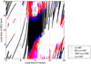 |
Fig. 14 Occurrence of SEDs as a function of the local time of Cassini and the local time of the storm cell F1. The different colors classify the SEDs by their emission angle α, i.e., the angle between the local zenith at the storm and Cassini. The black dots show all “direct” SEDs (α ≤ 90°), which propagate in a straight line from the storm to Cassini. The blue and red points show the over-the-horizon (OTH) SEDs in the range of 90° < α < 100° and 100° ≤ α < 135°, respectively. The magenta points show the extreme OTH SEDs with α ≥ 135°. Additionally, the dashed lines separate the day side from the night side (SED storm at 35° south has a solar zenith angle of 90° at local times of 5.6 h and 18.4 h.) For clarity of the plot we have restricted the data to latitudes of Cassini within ± 45° vfrom the equatorial plane, and we have excluded the time from 6–10 March due to the presence of another storm. |
5.4 The continuous SED detections of 6–10 March 2008
In the time interval 6–10 March 2008 (see Figs. 2 and 12) SEDs were continuously observed for nine consecutive Saturn rotations without episodic gaps. In those days the spacecraft was actually around apoapsis (at local times from 11.9 to 13.4 h), and in this case the explanation with the increased visibility range plus the over-the-horizon effect fails. The longitude range of the visible horizon is only ~ 140° during those days, and the α = 135° boundaries (most typical radio horizon) enclose a longitude range of ~ 255°, which is insufficient to explain the longitude ranges of 360° of the SED episodes. It also can not be related to pre- and post-episodes, which tended to occur with Cassini around local noon, since the SEDs of 6–10 March showed no restricted frequency range. It is likely that the storm cloud F2 started to emit SEDs in mid-March and not in early March, so that it also did not contribute to the continuous SED detections of 6–10 March. Nevertheless, an active SED storm F2 during 6–10 March, located ~25° eastward of F1, would have increased the SED longitude range by only ~25°. This is stillinsufficient to explain the observed SED longitude range of 360°. Spot S3 in Fig. 4 was located at 329° western longitude on 8 March. Similarly, its longitudinal separation from the main storm cell F1 (around 304° on 8 March) is also too narrow, and we rather suggested that the spot S3 showed no SED activity. Therefore, we conclude that there must be at least another storm cloud that is sufficiently separated in longitude with respect to the main storm cell F1 (at least by ~90°−120° depending on the storm latitude and the amount of the over-the-horizon effect). The images of amateur astronomers hardly show any other spots than those of storms F1, F2 and S3 in early March. The most likely candidate is a white spot observed by Tomio Akutsu around 40° western longitude on 11 March2008. However, it is not located in the storm alley, but in the Southern Tropical Zone (STrZ) at a planetocentric latitude around 25° south, and it would be the first time that an SED storm is located at such a latitude. Another smaller spot in the image of Tomio Akutsu is located around 49° western longitude at a high southern latitude (~60° south). Both spots can be seen in Fig. 15. They are located ~ 100° westward of storm F1 and thus could explain the continuous SED detections.
There is another extremely faint spot around 134° in western longitude imaged by A. Kazemoto on 7 March 2008. Its latitude is around 33° south, but it so faint that it is hardly discernible. Although its longitude would help explain the uninterrupted SED detections, its faintness does not suggest SED activity. (We note that a bright spot in the storm alley, supposedly observed around 33° longitude close to the central meridian of 25° at 23:20 UT on 3 March by Paulo Casquinha4, is most likely misdated. The positions of Rhea and Dione in his picture suggest that this observation was most probably made one day earlier.) Therefore, the most likely storms that added to the continuous SED detection of 6–10 March, are the white spots observed around 40°−50° western longitude by Tomio Akutsu on 11 March 2008.
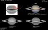 |
Fig. 15 Images from ground-based Saturn observations by Tomio Akutsu from 11 March 2008 with south being upward. The inverted image in the top row on the left shows the two candidate cloud features for the continuous SED detections of 6–10 March. An RGB image can be seen on the right side of the top row, and two infrared images are in the bottom row. |
5.5 Dark ovals
Dark ovals were observed during previous thunderstorms (Dyudina et al. 2007), and Baines et al. (2009) proposed that their dark color originates from carbon soot particles that could have been produced by dissociation of methane in the lightning channels. The soot particles might be attached to ammonia and ammonium hydrosulfide condensates, and they are thought to be transported to high altitudes above the 1 bar level by vertical convection. An alternative explanation has recently been given by Sromovsky et al. (2018), and they suggest that the dark ovals are less reflective because of reduced optical depth. Observations by Dyudina et al. (2007) have revealed the thunderstorm clouds as bright clouds that within a few weeks or so can be transformed into dark ovals. The suggested scenario is that the deep convection produces lightning and bright clouds consisting of large ammonia particles that rise up to the overlying cloud deck and push out the particles in that layer. When the convective pulse subsides, these large ammonia particles fall back leavingbehind less optical depth than the background clouds, which makes them appear darker (Sromovsky et al. 2018).
The dark ovals are absent in the first Cassini images of the storm from 6 December 2007, about ten days after the start of the SED storm. But, more and more dark ovals developed as the storm progressed (see e.g., Fig. 6), and the Cassini images of 19May 2008 show several of them spanning almost half the circumference of Saturn at the storm alley’s latitude. Most of the dark ovals drift westward and are located on the western side of the bright cloud from where they originate. Since the dark ovals were observed up to several weeks after the cessation of SED activity, one can conclude that they are not sources of lightning. Furthermore, assuming otherwise that the dark ovals would show lightning activity, their longitudinal placement half way around Saturn toward the end of storm F should have resulted in almost continuous SED detections without quiet periods between episodes. However, this was not the case. Finally, the dark ovals have a relatively stable shape, in stark contrast to the irregular morphology of the bright convective regions with SED activity. During SED storm F there was an exceptionally large dark oval that was identified as spot S3 even in ground-based images. Similarly, also this dark oval seemed to have no SED activity.
5.6 Splitting of convective system
Contemporaneous records from SED dynamic spectra and images enable us to attribute a remarkable decrease in the number of SEDs to a potential splitting of a convective cell. The following discussion refers to the splitting of a convective storm into a convective storm (bright cloud) and a dark oval. The feature S3, which appeared as faint spot in many ground-based images, also turned out to be an exceptionally large dark oval (see Sect. 3.2). Storm cell F2 is on a parallel drift line eastward of F1 in Fig. 4 with an almost constant separation of about 25° in longitude. This second storm cell of storm F seems to have developed independently and did not result from cell splitting.
In studies of terrestrial thunderstorms (Klemp 1987), convective cells tend to split when the CAPE (Convective Available Potential Energy) is high, and the wind shear is high in magnitude but low in directional strength. A single convective storm cell can split into two (or several) cells, and the daughter cells may either split further, or merge again to form a bigger cell than the parent cell. The splitting of convective cells has a remarkable signature in discharge frequency. Before the cell splitting, the lightning flash rate increases, which is due to the intensification of updrafts. An overshooting cloud top becomes observable, caused by a rapid increase in vertical cell growth. The cloud cell base shrinks in size. The exact opposite happens at the onset or after the cell splitting. At this later stage there is an intensification of downdraft; this reduces charge separation causing a decrease in flash rate. However, a decrease of the flash rate does not always indicate that a splitting has occurred, but the mature stage of thunderstorm development may have been reached, and decay by precipitation may have already started. A recent study of Earth’s atmosphere showcases several heavy thunderstorm events from a supercell, and how the lightning parameters change as a function of time before, during and after the onset of convective cell splitting (Meyer et al. 2013, and references therein). After the splitting takes place, two separate storm cells are formed. In the general terrestrial case, one cell moves to the right and the other moves to the left of the mean wind direction. In an ideal situation, they are mirror images to each other. In terrestrial thunderstorms occurring in the northern hemisphere, the left(right)-moving cell takes anticyclonic (cyclonic) updraft rotation. When the wind direction changes anticyclonically with increasing height, a right-moving cell dominates while the left-moving cell dissipates (Klemp & Wilhelmson 1978; Holton 2004). The dominant right-moving cell becomes the main source of electrical activity. The left-moving cell might be dissipating by precipitation. Rafkin & Barth (2015) applied these concepts to convective clouds on Titan, and in their model they found that for an increasing wind shear the storms transition to a multicellular regime.
It is not easy to transfer the situation from Earth to Saturn since we do not exactly know the change of wind direction with altitude for Saturnian thunderstorms. However, in Sect. 3.2 we have noted the difference in wind speed between a storm cell and the ambient flow, which suggests that a vertical wind shear is present in Saturn’s storm alley. There is a minimum in wind speed around 34° south latitude around which the convective storms are located. Their vorticity is mostly not clearly defined, parts of the storm located further northward and southward are moving with the ambient eastward flow. The centers of the storms are usually in the southward region (e.g., Vasavada et al. 2006). This usually leads to cyclonic vorticity further northward and anticyclonic vorticity further southward (for the southern hemisphere) as was shown in the images of the dragon storm by Dyudina et al. (2007). They showed in their Fig. 3 that the SED storm of September 2004 consisted mainly of three outbreaks α (DOY 253), β (DOY 257), and γ (DOY 269) characterized by bright white cloud features and a corresponding increase in SED activity. A closer look at the sequence of images in their Fig. 3 reveals that splitting processes also take place. Outbreak α seems to split around DOY 254 into a dark oval and a cloud feature that three days later becomes outbreak β. Similarly, around DOY 262 β splits into another dark oval and another cloud feature, which a week later becomes outbreak γ. In both cases, the dark ovals (no lightning activity, traced by lines in Fig. 3 of Dyudina et al. 2007) are further north and drift westward with respect to the bright cloud features (strong lightning activity) in the southeast.
The situation is similar for the splitting at the end of January 2008, when the spot S3 grows out of F1, see Fig. 4. Spot S3 is further west with respect to F1 and most likely shows no SED activity (see Sect. 5.3) whereas F1 returns as the main source of SED activity after a relatively quiet period of about two weeks. The decrease in lightning burst numbers after splitting can clearly be seen in Fig. 2 toward the end of January 2008. Despite the fact that the spacecraft is getting closer to Saturn on its inbound leg toward the periapsis on 27 January, the SED rate is decreasing. No more SEDs are observed for five days after periapsis on 27 January, and the electrical activity is very low afterwards for almost two weeks. We argue that this decrease in SED activity is caused by the splitting process, in which the dark oval S3 splits from F1. This dark oval was imaged as feature C by Cassini ISS on 4 March (see Fig. 6).
Other dark ovals might be related to SED activity minima and splitting processes, too. For example, feature B in Fig. 6, imaged slightly westward of storm cell F1 on 4 March (DOY 64), could be related to the SED minimum from the end of February 2008 (DOY 55–58), which is shown in Fig. 2. The dark oval very close to storm F2, which was imaged by Cassini ISS on 18 June in the right part of Fig. 6, might be related to the SED minimum around 15 June (see Fig. 3). The image of the storm alley from 23 April in Fig. 16 shows three large dark ovals westward of storm F1 with longitudinal distances of 10°−12° between each other. Storm cell F1 looks smaller and weaker compared tostorm cell F2 further eastward close to the limb. We now assume that dark ovals have typical drift rates of around ~ 0.9° per day, similar to the drift rate of spot S3. This means that the first dark oval at 333° western longitude might have spawned from storm cell F1 around 13 days prior to 23 April (DOY 114), the day the image of Fig. 16 was taken. So the splitting should have taken place around DOY 101, and one can see an SED minimum around DOY 100 in Fig. 3. The big dark oval at 345° western longitude could go back to a splitting process another 13 days earlier which would be around DOY 88. Indeed, there is a broad SED minimum around DOY 90 and starting at DOY 88. Finally, the dark oval at 355° western longitude should have spawned another 11 days earlier, around DOY 77, but there is no SED minimum in Fig. 3 on that day. However, there is a clear SED minimum around DOY 72, and a slightly smaller average drift rate of around 34∕42 = 0.81° per day for this dark oval could also relate it to an SED minimum.
It is not possible to check the relationship between all dark ovals and all SED minima throughout SED storm F for mainly two reasons:first, there is only a sparse ISS image coverage which does not allow to directly image the splitting process as it was done in Dyudina et al. (2007) with Cassini images almost every other day. Second, the existence of two storm cells at the same time after mid-March 2008 can hide some SED minima since we cannot distinguish between SEDs coming from F1 and F2. Nevertheless, the examples given above suggest that there is a relation between dark ovals, splitting processes and SED minima.
 |
Fig. 16 Contrast-enhanced image of Saturn’s storm alley made by Cassini ISS on 23 April 2008. The image with the file name W00044681.jpg was taken with filters CB2 and IRP0. There are three large dark ovals westward of storm cell F1, and we indicated their western longitudes. Storm cell F2 can also be seen further eastward close to the limb. |
6 Summary and conclusions
In this paper we analyzed a lightning storm that lasted seven and a half months in Saturn’s atmosphere at a planetocentric latitude of 35° south from the 27th of November 2007 until the 15th of July 2008. The Cassini RPWS (Radio and Plasma Wave Science) instrument observed about a quarter of a million SED events produced by lightning (or about half a million SED pixels, i.e., single time–frequency measurements) in three prevalent observational modes (survey mode, fast polarimeter survey mode, and direction-finding mode). The SEDs were organized in 439 SED episodes with a mean duration of ~ 5.6 h. For the first time, SEDs were observed from all local times during 25 Cassini orbits, and not only from Saturn’s morning side as in the previous storms. The number of SEDs observed in this storm depended largely on the distance of the Cassini spacecraft, and we showed that the SED maximum intensities decrease with distance squared. Hence, at large distances, a number of low intensity SEDs are below the background level. The average burst rate of detected SEDs was 1.8 SEDs per minute, and the maximum rate was about 1 SED per second. The SED polarization below 2 MHz was found to be mainly right-hand polarized with a median circular degree of −0.66 and a median linear degree of 0.29, similar to previous storms on the southern hemisphere.
The storm started as single convective cell, and this main convective cloud feature lasted from the beginning to the end of the storm. In mid-March 2008 a second bright storm cell appeared at the same latitude farther east, separated by ~ 25° in longitude. Both storm cells drifted westward with a similar rate of ~0.35° per Earth day, and both of them showed SED activity which resulted in an extended longitude range over which SEDs were observed in the second half of the storm starting in March 2008. This is the first time that Saturn lightning from two storm cells has been observed in parallel. There was even a third feature: it was fainter in the ground-based images and turned out to be a large dark oval in the Cassini images, and it most likely showed no SED activity. It split from the main storm cloud in late January 2008 and drifted westward with a rate of ~ 0.92° per day. It is very likely that this splitting process has led to the low SED activity of late January and early February 2008, similar to splitting processes in terrestrial thunderstorms. We found several examples of other dark ovals whose splitting from the main thunderstorm cell also caused minima in SED activity.
We note that the drift rate of the two convective storms of 0.35° per day corresponds to a westward velocity of 3.3 m/s, which is markedly slower than the environmental zonal wind. Only the third feature with the drift rate of 0.92° per day is compatible with the environmental wind, suggesting that it is non-convective. These examples show that the combined observationsof Cassini RPWS, the Cassini cameras, and ground-based observations by amateur astronomers have clearly enhanced our understanding of Saturnian thunderstorms.
Another important example for the usefulness of the combination of optical with radio observations is the so-called over-the-horizon effect: SEDs are detected when the storm is still beyond the visible horizon. This effect is thought to be due to a temporary trapping of SED radio waves below Saturn’s ionosphere (Zarka et al. 2006). This has previously been observed from Saturn’s morning side with the SED storm appearing from the night side, but here we show its existence for the first time also from the evening side with an SED storm that disappears toward the night side. We illustrated the over-the-horizon effect with plots (see Figs. 12 and 13) showing the longitude ranges of SED episodes as a function of time. The plots include lines showing the longitudes and times when the emission angle (angle between local zenith at SED storm and vector from SED storm to Cassini) is 90° (i.e., storm is at the limb as seen from Cassini) and 135° (i.e., an over-the-horizon effect of up to 45°). During many Cassini periapse passes the emission angle was consistently smaller than 135°, and in such cases there was uninterrupted SED detection over a few Saturn rotations.
Another new feature detected with SED storm F were the so-called pre- and post-episodes, and they were described as “isolated blobs” by Gautier (2013). Here we name them pre- and post-episode to distinguish if they occur before or after the main episode. Pre- and post-episodes are separated in time from the main episode, and typically they occur in a limited frequency range around 4 MHz. They were mostly observed with Cassini located at local noon. We found that the emission angles are around 135° during pre- and post-episodes, which means that they are manifestations of an extreme over-the-horizon effect. Another interesting feature of SED storm F is the uninterrupted SED detection from 6–10 March 2008 for nine consecutive Saturn rotations which cannot be explained by the over-the-horizon effect since Cassini was around apoapsis during this time. There must have been another storm present at this time, but it was not clearly seen in the images. A candidate event located at the right longitude (around 40° west) was found at a latitude of ~25° south, which would be an unusual latitude for an SED storm.
With Cassini now gone, future observations of Saturnian thunderstorms will have to rely on ground-based amateur astronomers and giant radio telescopes, which already observed Saturn’s strong lightning radio bursts in the past (Zakharenko et al. 2012; Konovalenko et al. 2013). For example, Saturn radio observations were made with the giant UTR-2 radio telescope in April 2018 while a bright polar cloud was present, but no evident SEDs were detected after a first inspection of the data.
Acknowledgements
Support from the Austrian Science Fund (FWF project P24325-N16) is gratefully acknowledged. P.Z. acknowledges support from CNES (French Space Agency) and the PNP & PNST programs from CNRS/INSU. The research at the University of Iowa was supported by NASA through contract 1415150 with the Jet Propulsion Laboratory. The authors also thank many amateur astronomers for their dedicated observations of Saturn, and especially Tomio Akutsu, Jean-Jacques Poupeau, and Maximo Suarez for the usage of their images in this paper. Cassini RPWS and ISS data are available via the Planetary Data System (PDS).
Appendix A: RPWS receiver modes for SED observations
The following three modes of the Cassini RPWS High Frequency Receiver (HFR) were prevalent in the observation of SED storm F. The first mode uses the Eu and Ev antennas (Gurnett et al. 2004; Cecconi & Zarka 2005) as a dipole (called Ex) in the HF2 band from 1825 to 16025 kHz with 143 steps of 100 kHz and a nominal integration time of 40 ms. From 325 to 1800 kHz (HF1 band) the dipole Ex as well as the monopole Ew are used in parallel in 60 steps of 25 kHz and an integration time of 80 ms. This mode is called the survey mode, and one frequency sweep is usually performed every 16 s. We call the duty cycle the percentage of time the receiver dwells at SED frequencies fSED, which we define as 1825 ≤ fSED ≤ 16 025 kHz, identical to the HF2 band in the survey mode. SED lower cutoff frequencies range from several hundreds of kHz (on the night side) to ~ 6 MHz (on the day side), depending on the peak electron density of the ionosphere (Fischer et al. 2011c). Our chosen lower limit (1825 kHz) of the SED frequency range corresponds to an average low frequency cutoff, and the upper limit (16 025 kHz) is the highest RPWS HFR frequency channel. The duty cycle for the survey mode is given by (143 × 35.3)∕16 000 = 0.3155 ≈ 0.32. This reflectsthe 143 frequency channels in HF2 with real (not nominal) integration time of 35.3 ms which are swept through every 16 s.
The second mode is the direction-finding (DF) mode which uses two pairs of monopoles successively. First, the auto- and cross-correlations of the pair Eu –Ew are measured, followed by the pair Ev –Ew. The nominal integration time in both cases is typically 80 ms, and one sweep is usually done every 32 s. The HF1 band from 325 to 4075 kHz uses a step size of 50 kHz, and in HF2 from 4025 to 16 025 kHz the frequency steps are usually 200 kHz. In both modes the instantaneous frequency bandwidth is 25 kHz. The duty cycle of the DF mode has been calculated by Fischer et al. (2006) to be 0.27.
A third mode was also used during SED storm F. One could call it a fast dipole–monopole survey mode which employed 315 steps of 50 kHz from 325 to 16025 kHz. The dipole Ex and monopole Ew were used in parallel throughout the whole frequency range with a faster nominal integration time of 20 ms. In this mode the duration of one sweep is somewhat variable ranging from 12 to 20 s. Using 16 s as an average, the duty cycle is (285 × 26.4)∕16 000 = 0.4703 ≈ 0.47, representing the 285 frequency channels from 1825 to 16 025 kHz with the real integration time of 26.4 ms.
Most SEDs were detected in the normal survey mode (~ 66.0%), followed by the fast survey mode (~20.4%), and the DF-mode (~13.6%). (Here we count full SEDs that can go over several frequency channels. The numbers for SED pixels, i.e., single time–frequency measurements, are slightly different and can be found in the beginning of Sect. 4.) The duty cycle can be used to calculate an extrapolated SED rate from the number of detected SEDs per time as done in Sect. 4.3. Taking into account the different modes the combined duty cycle of all storm F SEDs would be 0.660 × 0.32 + 0.136 × 0.27 + 0.204 × 0.47 = 0.344, resulting from survey mode, DF-mode, and fast survey mode, respectively.
Appendix B: SED extraction and polarization measurements
The SED detection algorithm of Fischer et al. (2006) is based on the SED statistical study of Zarka & Pedersen (1983) that defined and used for the first time an algorithm via comparison of the intensity of each pixel with that of surrounding pixels at the same frequency. The SEDs are extracted from the RPWS HFR data by using a threshold of four times the standard deviation (4σ) of the background radiation (Fischer et al. 2006). For the survey mode the 4σ-thresholds are 1.6 and 0.8 dB for bands HF1 and HF2, respectively. For the DF-mode it is 1.2 dB for both bands (HF1, HF2) of the HFR, and for the fast dipole–monopole survey mode the 4σ-threshold is 2.0 dB throughout the frequency range of HF1 and HF2. The SEDs not only have to be a certain threshold above the background, but also the same threshold above both neighboring pixels (neighbors at the same frequency but from the previous and the following sweep). This slightly reduces the number of detected low intensity SEDs as can be seen in the intensity distribution of Fig. 8, but it has the advantage that other emissions and interference are less likely included in the selection. The intensity thresholds are applied to the auto-correlation values measured by the dipole Ex (in the survey mode) or to the auto-correlation values of Eu and Ev (in the DF-mode), and not to the auto-correlation value measured by the Ew antenna. SEDs can extend over several frequency channels, and each single measurement at a certain time and frequency is called an SED pixel.
The SED polarization measurements were largely performed in the same way as described by Fischer et al. (2007a). Since the measurement error for polarization is much larger for small intensities (Cecconi & Zarka 2005), we required that the auto-correlation values of both antennas have to be above the intensity threshold in the respective mode. The calculated flux S of each pixel should also be greater than 10−16 V2 m−2 Hz−1. Another important factor limiting the accuracy is the angle β between thesource and the antenna plane. It should not be too small, and we took only SEDs with β >20° similar to Cecconi et al. (2006), and relaxing the more stringent criterion of β >40° of Fischer et al. (2007a). The center of Saturn was assumed to be the source direction which is a reasonable approximation. Another difference to the procedure described in Fischer et al. (2007a) is the usage of updated values for the antenna calibration according to Cecconi et al. (2009). The effective antenna directions were those of Vogl et al. (2004) for the so-called quasi-static case where the wavelength is still large compared to the dimensions of the spacecraft. Cecconi et al. (2009) found new values for the effective antenna length ratios with hx ∕hw = 2.45 ± 0.28, hu ∕hw = 1.19 ± 0.09, and hv ∕hw = 1.22 ± 0.18 for the high frequency part (HF1, HF2) of the HFR. These equations yield hu = 1.49 m, hv = 1.52 m, and hw = 1.25 m when the absolute effective length of the dipole is taken as hx = 3.06 m as was retrieved by Zarka et al. (2004). SEDs at and around frequencies of multiples of 100 kHz (± 6.25 kHz) were eliminated due to the interference at those frequencies which generally show a high degree of linear polarization. Furthermore, the SEDs from the frequency channels of 1343.75, 1743.75, 1750.00, and 1756.25 kHz were also eliminated due to enhanced degrees of linear polarization.
References
- Baines, K. H., Delitsky, M. L., Momary, T. W., et al. 2009, Planet. Space Sci., 57, 1650 [NASA ADS] [CrossRef] [Google Scholar]
- Balachandran, N. K. 1980, Mon. Weather Rev., 108, 804 [NASA ADS] [CrossRef] [Google Scholar]
- Cecconi, B., & Zarka, P. 2005, Radio Science, 40, RS3003 [Google Scholar]
- Cecconi, B., Zarka, P., & Kurth, W. S. 2006, in Planetary Radio Emissions VI, eds. H. O. Rucker, W. Kurth, & G. Mann (Austria: VÖAW), 37 [Google Scholar]
- Cecconi, B., Lamy, L., Zarka, P., et al. 2009, J. Geophys. Res. Space Phys., 114, A03215 [Google Scholar]
- Del Genio, A. D., Barbara, J. M., Ferrier, J., et al. 2007, Icarus, 189, 479 [NASA ADS] [CrossRef] [Google Scholar]
- Delcroix, M., & Fischer, G. 2010, in Eur. Planet. Sci. Congress 2010, 132 [NASA ADS] [Google Scholar]
- Desch, M. D., & Kaiser, M. L. 1981, Geophys. Res. Lett., 8, 253 [NASA ADS] [CrossRef] [Google Scholar]
- Dulk, G. A., Erickson, W. C., Manning, R., & Bougeret, J.-L. 2001, A&A, 365, 294 [NASA ADS] [CrossRef] [EDP Sciences] [Google Scholar]
- Dyudina, U. A., Ingersoll, A. P., Ewald, S. P., et al. 2007, Icarus, 190, 545 [NASA ADS] [CrossRef] [Google Scholar]
- Dyudina, U. A., Ingersoll, A. P., Ewald, S. P., et al. 2010, Geophys. Res. Lett., 37, L09205 [NASA ADS] [CrossRef] [Google Scholar]
- Fischer, G., Desch, M. D., Zarka, P., et al. 2006, Icarus, 183, 135 [NASA ADS] [CrossRef] [Google Scholar]
- Fischer, G., Gurnett, D. A., Lecacheux, A., Macher, W., & Kurth, W. S. 2007a, J. Geophys. Res. Space Phys., 112, A12308 [NASA ADS] [Google Scholar]
- Fischer, G., Kurth, W. S., Dyudina, U. A., et al. 2007b, Icarus, 190, 528 [NASA ADS] [CrossRef] [Google Scholar]
- Fischer, G., Gurnett, D. A., Kurth, W. S., et al. 2008, Space Sci. Rev., 137, 271 [NASA ADS] [CrossRef] [Google Scholar]
- Fischer, G., Dyudina, U. A., Kurth, W. S., et al. 2011a Planetary, Solar and Heliospheric Radio Emissions (PRE VII), 135 [Google Scholar]
- Fischer, G., Kurth, W. S., Gurnett, D. A., et al. 2011b, Nature, 475, 75 [NASA ADS] [CrossRef] [EDP Sciences] [Google Scholar]
- Fischer, G., Gurnett, D. A., Zarka, P., Moore, L., & Dyudina, U. A. 2011c, J. Geophys. Res. Space Phys., 116, A04315 [NASA ADS] [Google Scholar]
- García-Melendo, E., Pérez-Hoyos, S., Sánchez-Lavega, A., & Hueso, R. 2011, Icarus, 215, 62 [NASA ADS] [CrossRef] [Google Scholar]
- García-Melendo, E., Hueso, R., Sánchez-Lavega, A., et al. 2013, Nat. Geosci., 6, 525 [NASA ADS] [CrossRef] [Google Scholar]
- Gautier, A.-L. 2013, Ph.D. thesis, Observatoire de Paris [Google Scholar]
- Gautier, A.-L., Cecconi, B., Zarka, P., & Fischer, G. 2011, EPSC-DPS (Nantes, France) [Google Scholar]
- Gautier, A.-L., Cecconi, B., & Zarka, P. 2013, C. R. des Journées Scientifiques de l’URSI-France [Google Scholar]
- Gurnett, D. A., Kurth, W. S., Kirchner, D. L., et al. 2004, Space Sci. Rev., 114, 395 [NASA ADS] [CrossRef] [Google Scholar]
- Holton, J. R. 2004, An Introduction to Dynamic Meteorology (Oxford, UK: Academic Press), 535 [Google Scholar]
- Hueso, R., & Sánchez-Lavega, A. 2004, Icarus, 172, 255 [NASA ADS] [CrossRef] [Google Scholar]
- Hueso, R., Legarreta, J., Pérez-Hoyos, S., et al. 2010, Planet. Space Sci., 58, 1152 [NASA ADS] [CrossRef] [Google Scholar]
- Hunt, G. E., Godfrey, D., Muller, J.-P., & Barrey, R. F. T. 1982, Nature, 297, 132 [NASA ADS] [CrossRef] [Google Scholar]
- Ingersoll, A. P., Beebe, R. F., Conrath, B. J., & Hunt, G. E. 1984, Structure and Dynamics of Saturn’s Atmosphere, eds. T. Gehrels & M. S. Matthews (Tucson, AZ: University of Arizona Press), 195 [Google Scholar]
- Klemp, J. B. 1987, Ann. Rev. Fluid Mech., 19, 369 [NASA ADS] [CrossRef] [Google Scholar]
- Klemp, J. B., & Wilhelmson, R. B. 1978, J. Atmos. Sci., 35, 1097 [NASA ADS] [CrossRef] [Google Scholar]
- Konovalenko, A. A., Kalinichenko, N. N., Rucker, H. O., et al. 2013, Icarus, 224, 14 [NASA ADS] [CrossRef] [Google Scholar]
- Meyer, V. K., Höller, H., & Betz, H. D. 2013, Atmos. Chem. Phys., 13, 5137 [NASA ADS] [CrossRef] [Google Scholar]
- Pagaran, J. A., & Fischer, G. 2014, European Planetary Science Congress 2014, EPSC Abstracts, 9 [Google Scholar]
- Porco, C. C., West, R. A., Squyres, S., et al. 2004, Space Sci. Rev., 115, 363 [NASA ADS] [CrossRef] [Google Scholar]
- Porco, C. C., Baker, E., Barbara, J., et al. 2005, Science, 307, 1243 [NASA ADS] [CrossRef] [Google Scholar]
- Rafkin, S. C. R., & Barth, E. L. 2015, J. Geophys. Res. Planets, 120, 739 [NASA ADS] [CrossRef] [Google Scholar]
- Rakov, V. A., & Uman, M. A. 2003, Lightning (Cambridge: Cambridge University Press), 698 [Google Scholar]
- Read, P. 2011, Nature, 475, 44 [NASA ADS] [CrossRef] [Google Scholar]
- Sanchez-Lavega, A., & Battaner, E. 1987, A&A, 185, 315 [NASA ADS] [Google Scholar]
- Sánchez-Lavega, A., del Río-Gaztelurrutia, T., Hueso, R., et al. 2011, Nature, 475, 71 [NASA ADS] [CrossRef] [Google Scholar]
- Sánchez-Lavega, A., Fischer, G., Fletcher, L. N., et al. 2019, The Great Saturn Storm of 2010-2011 (Cambridge: Cambridge University Press) [Google Scholar]
- Sayanagi, K. M., Dyudina, U. A., Ewald, S. P., et al. 2013, Icarus, 223, 460 [NASA ADS] [CrossRef] [Google Scholar]
- Sromovsky, L. A., Revercomb, H. E., Krauss, R. J., & Suomi, V. E. 1983, J. Geophys. Res., 88, 8650 [NASA ADS] [CrossRef] [Google Scholar]
- Sromovsky, L. A., Baines, K. H., & Fry, P. M. 2018, Icarus, 302, 360 [NASA ADS] [CrossRef] [Google Scholar]
- Vasavada, A. R., Hörst, S. M., Kennedy, M. R., et al. 2006, J. Geophys. Res. Planets, 111, E05004 [NASA ADS] [CrossRef] [Google Scholar]
- Vogl, D. F., Cecconi, B., Macher, W., et al. 2004, J. Geophys. Res. Planets, 109, A09S17 [Google Scholar]
- Warwick, J. W., Pearce, J. B., Evans, D. R., et al. 1981, Science, 212, 239 [NASA ADS] [CrossRef] [PubMed] [Google Scholar]
- Warwick, J. W., Evans, D. R., Romig, J. H., et al. 1982, Science, 215, 582 [NASA ADS] [CrossRef] [Google Scholar]
- Zakharenko, V., Mylostna, C., Konovalenko, A., et al. 2012, Planet. Space Sci., 61, 53 [NASA ADS] [CrossRef] [Google Scholar]
- Zarka, P. 1985, Icarus, 61, 508 [NASA ADS] [CrossRef] [Google Scholar]
- Zarka, P., & Pedersen, B. M. 1983, J. Geophys. Res., 88, 9007 [NASA ADS] [CrossRef] [Google Scholar]
- Zarka, P., Cecconi, B., & Kurth, W. S. 2004, J. Geophys. Res. Space Phys., 109, A09S15 [Google Scholar]
- Zarka, P., Cecconi, B., Denis, L., et al. 2006, in Planetary Radio Emissions VI, eds. H. O. Rucker, W. Kurth, & G. Mann (Austria: VÖAW), 111 [Google Scholar]
Not shown here, see e.g., the image of Carmelo Zannelli on http://pvol2.ehu.eus/pvol2/.
All Figures
|
Fig. 1 Illustration of Cassini’s trajectory (about 25 orbits) during the SED storm from 27 November 2007 (marked by a triangle) until 15 July 2008 (marked by a square) in Saturn’s equatorial system. The trajectory is colored from blue (low inclination orbits) to red (high inclination orbits) to follow its temporal evolution. Saturn is schematically illustrated at the origin of the coordinate system with the z-axis along Saturn’s rotation axis, and the positive x-axis points toward the Sun in a plane formed by the rotation axis and the line from Saturn to the Sun. |
| In the text | |
|
Fig. 2 Number of detected SEDs per hour in logarithmic scale as a function of time (in DOY 2007/2008, upper panel), and radial distance of Cassini as function of time (lower panel). This figure gives the first part of SED storm F from late November 2007 until 9/10 March 2008. The periapse times are marked by dotted vertical lines in both panels. The horizontal lines at the top indicate times when SED episodes lasted for a full Saturn rotation. |
| In the text | |
|
Fig. 3 Number of detected SEDs per hour as a function of time (in DOY 2008, upper panel), and distance of Cassini as function of time (lower panel). This figure gives the second part of SED storm F from 10 March until 15 July 2008. Similar to the previous figure, the periapse times are marked by dotted vertical lines in both panels, and the horizontal lines indicate times when SED episodes lasted for a full Saturn rotation. |
| In the text | |
|
Fig. 4 Location of cloud features as a function of time as imaged by Cassini (diamonds) and ground-based amateur astronomers (dots). All longitudes in this figure and paper are western longitudes in degrees of Voyager SLS. The x-axis was inverted to have larger western longitudes on the left side. The y-axis goes from the start of storm F (27 November 2007) until its end (15 July 2008) with the start of the storm on the top. The different colors denote the storm cells F1, F2 and spot S3 as discussed in the text. |
| In the text | |
|
Fig. 5 Amateur images of Saturn with south pointing upward from February and March 2008. Left panel: RGB image of Saturn taken by Jean-Jacques Poupeau on 23 February 2008, 23:47 UT. The prominent cloud feature close to the central meridian is the storm cell F1. The faint cloud feature about 20° westward of F1 is marked with red lines, and this is spot S3 as discussed in the text. Right panel: Saturn image in green filter taken by Maximo Suarez on 6 March 2008, 23:20 UT. The magnified inset panel shows four features named A, B, C, and D, where the latter is questionable. Feature A corresponds to storm cell F1 with feature B being a westward extension of A. Feature C corresponds to spot S3. |
| In the text | |
|
Fig. 6 Cassini ISS images from 4 March 2008 (left panel), and 18 June 2008 (right panel). The left image shows mainly one bright storm cloud, whereas there are two bright storms in the right image. In the 4 March image the bright storm F1 is located at 302° western longitude. We have marked the features A, B, and C corresponding to the features shown in the right panel of Fig. 5, that were imaged by M. Suarez two days later. This shows that spot S3 is actually a large dark oval. The 18 June image shows two bright spots at 310.3° (F2) and at 343.4° (F1) western longitude, with the older storm cell F1 further west (left) than the younger storm cell F2. All spots are located around ~35° south planetocentric latitude. The left image (file name W00043078.jpg) was taken with filters CB3 and CL2, and the right image (file name W00046585.jpg) was taken with filters CB3 and IRP0 (Images by NASA/JPL/SSI). |
| In the text | |
|
Fig. 7 Intensities of SED storm F pixels as a function of distance between storm F1 and Cassini. The data was divided in 18 distance intervals with a bin size of 2 RS, centered at the values of 3, 5, 7,... 37 RS. For each interval we calculated the median intensity value (50% percentile, blue curve), the 80% percentile (green curve), the 95% percentile (red curve), and the maximum (100% percentile, cyan curve). The gray line represents an inverse-square law ( |
| In the text | |
|
Fig. 8 Distribution of SED pixel intensities of storm F with a bin size of 0.4 dB. The gray bars represent all SED pixels, and the black bars show the distribution of pixels from a single SED episode, the closest approach episode of 10 May 2008 before noon. For a better visibility the black bars of the single episode are magnified by a factor of 10 with respect to the scale on the ordinate. The dashed fitted curve is given by the two-term exponential model of Eq. (4). |
| In the text | |
|
Fig. 9 Distribution of SED storm F episode durations in half hour bins in a stacked histogram. The distribution contains 522 values, which includes 439 regular episodes, 49 pre-episodes, and 34 post-episodes. |
| In the text | |
|
Fig. 10 Sample episodes with pre- and post-episodes. Left panel: storm episode F298 with a pre-episode. Right panel: episode F036 with a post-episode. We show the extracted SEDs displayed versus time (in hours of SCET, spacecraft event time) and frequency. The frequency range (with linear scale from 1.8 to 16.2 MHz) in the left and right panels are exactly the same. In the left panel nine hours are displayed, and in the right panel it is seven hours. The colors indicate the SED pixel intensities in dB above background. |
| In the text | |
|
Fig. 11 Local time and kronocentric latitude of Cassini during the recording of pre-episodes (magenta stars) and post-episodes (cyan stars). The black dots show the position of Cassini in local time and latitude from 27 November 2007 until 15 July 2008 with a resolution of one dot per hour. |
| In the text | |
|
Fig. 12 Subspacecraft western longitude ranges of SED episodes from the end of November 2007 until mid-March 2008. The western longitude ranges are displayed as almost vertical black lines. These lines are dotted for SED episodes with less than 20 SEDs, dashed for episodes with more than 20 but less than 200 SEDs, and solid for episodes with greater than or equal to 200 SEDs. For each episode the red asterisk marks the western longitude at the center time of the respective episode (i.e., mean time of all SEDs from this episode). The western longitude ranges of pre-episodes are colored in magenta, and the ranges of post-episodes are colored in cyan. The almost horizontal red lines indicate the western longitudes of the storm cells F1 (red solid line), F2 (red dashed line), and S3 (red dottedline), respectively. Similar to Fig. 2, the black horizontal lines on top indicate times when SED episodes lasted for a full Saturn rotation, which means that the western longitude range goes up to 360° for such episodes. Additionally, the interval of continuous SED detections from 6–10 March is indicated by black vertical dot-dashed lines. The green dots mark the times and subspacecraft western longitudes when the emission angle α is 90°, and the blue dots indicate the times and western longitudes for α = 135°. The angle α is defined as the angle between the local zenith at the location of SED storm F1 and the vector from the SED storm to Cassini. More detailed explanations can be found in the text. |
| In the text | |
|
Fig. 13 Subspacecraft western longitude ranges of SED episodes from mid-March until mid-July 2008. The figure has the same formatas the previous Fig. 12. |
| In the text | |
|
Fig. 14 Occurrence of SEDs as a function of the local time of Cassini and the local time of the storm cell F1. The different colors classify the SEDs by their emission angle α, i.e., the angle between the local zenith at the storm and Cassini. The black dots show all “direct” SEDs (α ≤ 90°), which propagate in a straight line from the storm to Cassini. The blue and red points show the over-the-horizon (OTH) SEDs in the range of 90° < α < 100° and 100° ≤ α < 135°, respectively. The magenta points show the extreme OTH SEDs with α ≥ 135°. Additionally, the dashed lines separate the day side from the night side (SED storm at 35° south has a solar zenith angle of 90° at local times of 5.6 h and 18.4 h.) For clarity of the plot we have restricted the data to latitudes of Cassini within ± 45° vfrom the equatorial plane, and we have excluded the time from 6–10 March due to the presence of another storm. |
| In the text | |
|
Fig. 15 Images from ground-based Saturn observations by Tomio Akutsu from 11 March 2008 with south being upward. The inverted image in the top row on the left shows the two candidate cloud features for the continuous SED detections of 6–10 March. An RGB image can be seen on the right side of the top row, and two infrared images are in the bottom row. |
| In the text | |
|
Fig. 16 Contrast-enhanced image of Saturn’s storm alley made by Cassini ISS on 23 April 2008. The image with the file name W00044681.jpg was taken with filters CB2 and IRP0. There are three large dark ovals westward of storm cell F1, and we indicated their western longitudes. Storm cell F2 can also be seen further eastward close to the limb. |
| In the text | |
Current usage metrics show cumulative count of Article Views (full-text article views including HTML views, PDF and ePub downloads, according to the available data) and Abstracts Views on Vision4Press platform.
Data correspond to usage on the plateform after 2015. The current usage metrics is available 48-96 hours after online publication and is updated daily on week days.
Initial download of the metrics may take a while.