| Issue |
A&A
Volume 620, December 2018
|
|
|---|---|---|
| Article Number | A143 | |
| Number of page(s) | 18 | |
| Section | Galactic structure, stellar clusters and populations | |
| DOI | https://doi.org/10.1051/0004-6361/201833951 | |
| Published online | 11 December 2018 | |
The VMC Survey
XXXII. Pre-main-sequence populations in the Large Magellanic Cloud
1
Lennard-Jones Laboratories, School of Chemical and Physical Sciences, Keele University, ST5 5BG, UK
e-mail: This email address is being protected from spambots. You need JavaScript enabled to view it.
2
European Southern Observatory, Karl-Schwarzschild-Str. 2, 85748 Garching bei München, Germany
3
Leibniz-Institut für Astrophysik Potsdam, An der Sternwarte 16, 14482 Potsdam, Germany
4
Dipartimento di Fisica e Astronomia, Universitá di Padova, Vicolo dell’Osservatorio 2, 35122 Padova, Italy
5
Osservatorio Astronomico di Padova – INAF, Vicolo dell’Osservatorio 5, 35122 Padova, Italy
6
ICRAR, M468, University of Western Australia, 35 Stirling Hwy, 6009 Crawley, Western Australia, Australia
7
INAF-Osservatorio di Astrofisica e Scienza dello Spazio di Bologna, Via P. Gobetti 93/3, 40129 Bologna, Italy
8
Department of Physics and Astronomy, Macquarie University, Balaclava Road, Sydney, NSW 2109, Australia
9
Research Centre for Astronomy, Astrophysics and Astrophotonics, Macquarie University, Balaclava Road, Sydney, NSW 2109, Australia
10
International Space Science Institute–Beijing, 1 Nanertiao, Zhongguancun, Hai Dian District, Beijing 100190, PR China
11
INAF-Osservatorio Astronomico di Capodimonte, Via Moiariello 16, 80131 Naples, Italy
12
Kavli Institute for Astronomy & Astrophysics and Department of Astronomy, Peking University, Yi He Yuan Lu 5, Hai Dian District, Beijing 100871, PR China
Received:
25
July
2018
Accepted:
8
October
2018
Abstract
Context. Detailed studies of intermediate- and low-mass pre-main-sequence (PMS) stars outside the Galaxy have so far been conducted only for small targeted regions harbouring known star formation complexes. The VISTA Survey of the Magellanic Clouds (VMC) provides an opportunity to study PMS populations down to solar masses on a galaxy-wide scale.
Aims. Our goal is to use near-infrared data from the VMC survey to identify and characterise PMS populations down to ∼1 M⊙ across the Magellanic Clouds. We present our colour–magnitude diagram method, and apply it to a ∼1.5 deg2 pilot field located in the Large Magellanic Cloud.
Methods. The pilot field is divided into equal-size grid elements. We compare the stellar population in every element with the population in nearby control fields by creating Ks/(Y−Ks) Hess diagrams; the observed density excesses over the local field population are used to classify the stellar populations.
Results. Our analysis recovers all known star formation complexes in this pilot field (N 44, N 51, N 148, and N 138) and for the first time reveals their true spatial extent. In total, around 2260 PMS candidates with ages ≲10 Myr are found in the pilot field. PMS structures, identified as areas with a significant density excess of PMS candidates, display a power-law distribution of the number of members with a slope of −0.86 ± 0.12. We find a clustering of the young stellar populations along ridges and filaments where dust emission in the far-infrared (FIR) (70 μm–500 μm) is bright. Regions with young populations lacking massive stars show a lower degree of clustering and are usually located in the outskirts of the star formation complexes. At short FIR wavelengths (70 μm,100 μm) we report a strong dust emission increase in regions hosting young massive stars, which is less pronounced in regions populated only by less massive (≲4 M⊙) PMS stars.
Key words: techniques: photometric / galaxies: individual: LMC / galaxies: star formation / stars: pre-main sequence / stars: statistics
© ESO 2018
1. Introduction
The Magellanic Clouds (MCs) are nearby, interacting, gas-rich galaxies with metallicities lower than typically encountered in the Milky Way (Stanimirović et al. 2004; Besla et al. 2012). With moderate distances of 50 ± 2 kpc for the Large Magellanic Cloud (LMC; de Grijs et al. 2014) and 61.9 ± 0.6 kpc for the Small Magellanic Cloud (SMC; de Grijs & Bono 2015), they provide a great opportunity to study resolved star formation down to the scales of individual young stellar objects under different environmental conditions than those found in the Galaxy. The LMC has an apparent size on the sky of approximately 5.4° × 4.6° (Cook et al. 2014) and is seen almost face-on (van der Marel & Cioni 2001). Its depth is 4.0 ± 1.4 kpc and 3.44 ± 1.16 kpc in the bar region and the disc, respectively (Subramanian & Subramaniam 2009), leading to relatively small distance modulus variations among its stellar members. The mean metallicity of the LMC is approximately half of the solar metallicity (Russell & Dopita 1992), which places it close to the mean metallicity of the interstellar medium during the time of peak star formation in the Universe (Pei et al. 1999).
The first studies of young stellar populations within the MCs were published over half a century ago (Westerlund 1961; Bok 1964). Lucke & Hodge (1970) created a catalogue of 122 OB associations in the LMC, based on observations at optical wavelengths down to mV ≈ 16 mag, which corresponds at the LMC distance to an ∼11 M⊙ main-sequence star of age 10 Myr (Bressan et al. 2012). The advent of sensitive CCD detector arrays improved the detection limit so that more detailed studies of the stellar content of associations became possible (e.g. Massey et al. 1989a,b). A huge leap in sensitivity and resolution was provided by the Hubble Space Telescope (HST). Optical imaging studies of young clusters and OB associations in both galaxies have found evidence of extensive pre-main-sequence (PMS) populations well below the solar mass regime (e.g. Gilmozzi et al. 1994; Panagia et al. 2000; Gouliermis et al. 2006a,b, 2007, 2011). Analysis of the PMS populations in the 30 Doradus region, revealed by the Hubble Tarantula Treasury Project (HTTP; Sabbi et al. 2013), allowed Cignoni et al. (2015) to reconstruct the star formation history of the complex. They also reported that low-mass stars can form in starburst regions as well as in low-density environments. Overall, the observed initial mass function (IMF) in the LMC is consistent with that of the Galaxy (e.g. Da Rio et al. 2009; Liu et al. 2009a,b). Spezzi et al. (2012) and De Marchi et al. (2013) used narrow-band photometry with an Hα-filter to identify PMS objects actively undergoing mass accretion. Both studies found that PMS stars in the MCs have higher mass accretion rates than stars of similar mass in the Galaxy, which might be an effect of metallicity. All these HST-studies targeted individual associations and/or star-forming complexes, uncovering the young stellar populations down to masses as low as ∼0.3 M⊙
In contrast, large-scale photometric surveys of the LMC and/or SMC give a galaxy-wide overview of the stellar populations. They allow investigating the large-scale distribution of star-forming complexes and their relationship with the underlying gas and dust distribution. Optical imaging was performed by the Magellanic Cloud Photometric Survey (MCPS; Zaritsky et al. 2002, 2004), and near-infrared (NIR) images were provided by the 2 Micron All Sky Survey (2MASS; Skrutskie et al. 2006). Mid- and far-infrared (MIR, FIR) imaging was performed by the Spitzer Space Telescope (Spitzer; Werner et al. 2004) and the Herschel Space Observatory (Herschel; Pilbratt et al. 2010) as part of two legacy surveys (SAGE and SAGE-SMC: Meixner et al. 2006; Gordon et al. 2011; HERITAGE: Meixner et al. 2013). These surveys provided a comprehensive overview of the high-mass young stellar content and their spatial distribution, but they lack the depth and resolution for studying the intermediate- and low-mass young stellar population.
The VISTA Survey of the Magellanic Clouds (VMC; Cioni et al. 2011) provides a significant improvement in depth and resolution. Its data are being used, amongst other works, to characterise the stellar content of the MCs. Piatti et al. (2014) analysed the colour–magnitude diagrams (CMDs) of known clusters in the LMC, while Piatti et al. (2016) used stellar over-densities to detect new stellar clusters in the SMC with ages between log(t/yr) ∼ 7.5−9.0. Sun et al. (2017a,b, 2018) used upper main-sequence (UMS) stars to trace large-scale structures in major star formation complexes in the LMC and SMC. They found that the size and mass distributions follow a power law, which supports hierarchical star formation governed by turbulence. Less massive PMS stars, due to their extended PMS phase (Baraffe et al. 2015), provide valuable information about the recent star formation history (see Gouliermis 2012, for an overview). Identifying the PMS populations, including star formation sites only composed of intermediate- and low-mass stars, can thus reveal the full galaxy-wide extent of recent star formation.
We present an automated method that uses the capabilities of the VMC to detect intermediate- and low-mass (1 M⊙ ≲ M* ≲ 4 M⊙) PMS populations. The method is based on a colour–magnitude Hess diagram (Hess CMD) analysis, which includes corrections for reddening and completeness, in order to distinguish young populations from the field. This paper describes the development of this method as well as its application to a ∼1.5 deg2 region in the LMC. The chosen pilot field contains well-studied OB associations with known PMS populations that are used to calibrate and fine-tune the method. The paper is organized as follows: Sect. 2 gives an overview of the VMC survey and the data used in this work. Section 3 describes how we deal with the contamination from old field stars, while Sect. 4 explains in detail the strategy we devised to identify and categorise young populations. In Sect. 5 we present tests using synthetic and literature clusters to evaluate the sensitivity of the method for the cluster age and mass. We show in Sect. 6 first results based on the application of our method to the LMC pilot field and discuss the properties of the identified young low-mass populations. Finally, we present a summary and our main conclusions in Sect. 7.
2. VISTA/VMC survey data selection
The data used in this work are part of the VMC, which is an ESO public survey carried out with the VISTA InfraRed CAMera (VIRCAM) instrument on the 4.1 m VISTA telescope (Sutherland et al. 2015). The observing strategy of the VMC involves multi-epoch imaging of tiles across the Magellanic System in the Y (1.02 μm), J (1.25 μm), and Ks (2.15 μm) bands. One tile almost uniformly covers an area of ∼1.5 deg2 as a result of combining six offset paw-print images in order to fill the gaps between the 16 VIRCAM detectors. Overall, the survey consists of 110 tiles that cover an area of ∼ 170 deg2. Upon completion, every tile will have been observed at 3 epochs in the Y and J bands, and 12 epochs in the Ks band. The exposure time per epoch is 800 s in Y and J, and 750 s in Ks, leading to total exposure times of 2400 s (Y, J) and 9000 s (Ks).
We chose as a pilot field the area covered by the tile LMC 7_5. Its central coordinates are α (J2000) ≈ 81°493 and δ(J2000) ≈ −67°895, which is approximately 1°7 to the north-west of the Tarantula Nebula and to the north of the LMC bar. The coordinate range covered by this tile is approximately 80°0 ≲ α ≲ 83°0 and −68°6 ≲ δ ≲ −67°2. Figure 1 shows the location of tile LMC 7_5 within the wider environment of the LMC. This field harbours LHA 120-N 44 and LHA 120-N 51 (Henize 1956), two large star-forming complexes (e.g. Carlson et al. 2012) that are discussed in more detail in Sect. 6.1. They include massive OB associations like LH 60 and LH 63, in which significant populations of intermediate- and low-mass PMS stars down to ∼0.5 M⊙ have been identified (Gouliermis et al. 2011). Several older clusters with ages between 10 Myr and 1 Gyr are also found in this field (e.g. Glatt et al. 2010; Popescu et al. 2012).
We use a photometric catalogue obtained by performing point spread function (PSF) photometry on stacked PSF-homogenized images (Rubele et al. 2012, 2015). Previous studies have shown that PSF photometry recovers more sources in crowded regions than aperture photometry (e.g. Tatton et al. 2013). PSF photometry results in deeper and more complete catalogues especially in areas with active or very recent star formation. We tested this by comparing the PSF photometry data with aperture photometry data, reduced and calibrated with the VISTA Data Flow System (VDFS) pipeline (Irwin et al. 2004; González-Fernández et al. 2018) and retrieved from the VISTA Science Archive (VSA1; Cross et al. 2012) for six circular regions with a radius of 2′. Three regions contain young OB associations (LH 54, LH 60, and LH 63), while the other three showed no sign of recent star formation activity or stellar over-densities. The PSF photometry detects ∼1.4 times more sources in regions without active star formation, and ∼1.6 times more sources in the regions containing the three young associations. In addition, the PSF catalogues provide estimates of the local completeness for every filter based on artificial star tests (Rubele et al. 2012). These estimates are used to correct for differences in the completeness between stellar populations from different regions (Sect. 3.3). For the PSF catalogue a completeness of 50% is typically reached at Y ≈ 21.4 mag, J ≈ 21.3 mag, and Ks ≈ 20.6 mag. The 5σ magnitude limits are Y ≈ 22.3 mag, J ≈ 21.9 mag, and Ks ≈ 20.9 mag (for the nominal aperture photometry magnitude limits, see Cioni et al. 2011). Using the mean reddening in LMC 7_5 (E(Y−Ks) ≈ 0.18 mag; Tatton et al., in prep.), the PSF 5σ limits correspond to ∼0.7 M⊙ and ∼1.3 M⊙ for ages of 1 Myr and 10 Myr, respectively.
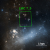 |
Fig. 1. Digitized Sky Survey (DSS) image showing the location of the pilot field (highlighted in green) within the wider LMC environment. North is up and east is to the left. |
3. Constructing differential Hess diagrams
To identify young stellar populations in the pilot field, we use the star positions in the CMD, which are indicative of their masses and ages. CMD-based methods are widely used to analyse clusters of all ages (e.g. Da Rio et al. 2009; Rubele et al. 2011; Girardi et al. 2013; Niederhofer et al. 2017). In general, observations towards clusters or associations are contaminated by the dispersed field population; it is thus necessary to apply a robust decontamination procedure. In this paper we work with Ks/(Y − Ks) CMDs, since the longer wavelength baseline makes different populations easier to distinguish.
3.1. CMD density diagrams
We start by spatially dividing the pilot field into a grid (see Fig. 2). Every grid element is circular, and the distance between the centres of two neighbouring elements is one grid element radius. The resulting overlap ensures that every location is covered by the grid. It also reduces the chance that a young cluster or association is split up between two or more neighbouring grid elements. The grid radius is a very important parameter, and it is the subject of extensive testing in this study (see Sect. 5). We defined grids with radii of r = {90″,75″,60″,50″,40″}. Individual Ks/(Y − Ks) CMDs are constructed for each grid element. The CMDs are then smoothed using a Gaussian kernel, resulting in a 2D density map of the stellar distribution in colour–magnitude space. The widths of the kernels define the colour–magnitude resolution of our density maps; they must be small enough to highlight the distribution of different stellar populations in the CMD, but large enough to be robust against small number statistics. We apply an adaptive kernel width that depends on the number of stars in a grid element (N*, ge) and on the photometric errors as follows:
 (1)
(1)
 (2)
(2)
where 〈N*〉 is the median number of stars in the coarsest grid. If the mean photometric error within the kernel, ΔKs > σKs we adopt σKs = ΔKs. The width values are typically in the ranges 0.1 mag < σY − Ks < 0.2 mag and 0.2 mag < σKs < 0.4 mag. Kernel width maxima of σY − Ks = 0.2 mag and σKs = 0.4 mag are set to prevent smoothing over too large CMD regions. The smoothing procedure results in a Hess CMD for every grid element. Figure 3 shows representative CMDs (top) and Hess CMDs (bottom) for two grid elements containing mostly old field stars (left) and a star-forming region (right), as shown by the overplotted PARSEC2 isochrones (Bressan et al. 2012).
3.2. Control field selection
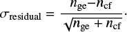
To decontaminate each grid element from field stars, we use offset control fields that closely resemble the local field population. The total size of the pilot field precludes the use of a single control field for the whole tile, since the typical field population changes over such large spatial scales. Hence it is necessary to define control fields individually for every grid element. The approach is as follows: we count stars within the UMS and PMS regions of the CMD (shown in Fig. 3) for all grid elements within a distance of 1000″ from the grid element being analysed. The UMS and PMS regions are defined primarily using PARSEC isochrones. Furthermore, the red limit for the PMS region excludes background galaxies (Kerber et al. 2009), while the blue edge excludes most old field stars. The boundary at bright magnitudes is generous enough to allow for effects like PMS variability and IR excesses, and the lower boundary is imposed by the sensitivity of the survey. The CMD of a typical LMC field population is expected to have significantly fewer stars within the UMS and PMS regions than that of an area dominated by young stars. Star counts can thus identify grid elements that are control field candidates. An example control field search area is depicted in Fig. 2. The number of grid elements within this area varies, depending on the size of the elements; the coarsest grid (90″ radius) contains around 360 grid elements. We create histograms of the star counts for both the UMS and PMS regions and approximate these with Gaussian distributions.
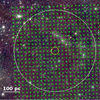 |
Fig. 2. VISTA RGB composite with Y (1.02 μm) in blue, J (1.25 μm) in green, and Ks (2.15 μm) in red showing the north-eastern corner of the pilot field. Green crosses are placed at the centres of the grid elements (90″ radius in this instance). The small yellow circle highlights an example grid element, while the large white circle shows the area searched to identify suitable control field regions (see text). |
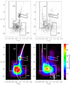 |
Fig. 3. Top: CMDs of two example grid elements. Boxes indicate the UMS and PMS regions used in the control field selection, as well as the RC region used to determine the mean extinction (see Sect. 3.2 for details). The slope of the RC selection box is defined by the reddening vector. Bottom: corresponding Hess CMDs. Thin solid lines are PARSEC isochrones (Bressan et al. 2012) for log(t/yr) ∈ [9.5, 9.6, 9.7, 9.8] and Z = 0.0033 (left panel), and log(t/yr) ∈ [6.0, 6.1, 6.2, 6.3, 6.4, 6.5, 6.6, 6.7, 6.8] and Z = 0.008 (right panel). The assumed metallicities are typical for the age ranges (Rubele et al. 2012; Tatton et al. 2013). The isochrones are shifted by a distance modulus of 18.49 mag (de Grijs et al. 2014), and an extinction correction derived from the RC analysis (see text) is applied. The dotted line marks the typical 50% completeness level. |
In addition, the mean extinction towards every grid element within the control field search area is determined by using the mean observed colour of red clump (RC) stars. These are evolved stars with well-constrained luminosities, and thus the RC is often used for distance and reddening measurements (e.g. Paczyński & Stanek 1998; Tatton et al. 2013). Although population effects change the absolute magnitude of RC stars (Girardi & Salaris 2001), any variations on ≪ kpc scales are generally dominated by distance differences and reddening. The selection box for the RC is also indicated in Fig. 3. Its slope of 0.434 is calculated based on the relative extinctions for VISTA filters, AY/AV ≈ 0.390 and AKs/AV1 ≈ 0.118 (Catelan et al. 2011). The Y − Ks colour limits were chosen to keep the contamination by non-RC objects low, while still covering typical LMC reddening values (Rubele et al. 2012; Tatton et al. 2013). Assuming an intrinsic RC colour of (Y − Ks)0 =0.84 mag (Tatton et al. 2013), we probe extinction values up to AV ≈ 4.26 mag. The magnitude limits are such as to be insensitive to the small distance variations due to the depth of the LMC along the line of sight. We create a histogram of all mean extinction values within the control field search area, and fit it with a Gaussian distribution. Across the pilot field, the mean extinction is AV ≈ 0.7 mag, consistent with another determination using the RC method (AV ≈ 0.66 mag; Tatton et al., in prep.).
A grid element is considered a reliable control field candidate if its UMS and PMS counts, and mean extinction are within 1σ from the mean value of the respective Gaussian distributions. Usually, over 100 suitable control field candidates are found within any given 1000″ search area (61 is the minimum). The algorithm automatically selects the N nearest control field candidates and combines them into a master control field. The chosen value for N depends on the grid radius: N = 10, 14, 20, 28, and 40 for the 90″, 75″, 60″, 50″, and 40″ grids, respectively. These values provide a good balance between computing time and well-sampled control field populations.
3.3. CMD residuals and significance maps
In order to compare the stellar content of a grid element to that of the respective master control field, it is necessary to correct for differences in the reddening, since reddened main-sequence stars can occupy the same region in the CMD as PMS stars. Using the mean extinction values determined in Sect. 3.2 is not appropriate since it would not account for differential reddening. Instead, the magnitudes of the stars in the control fields are individually corrected. We start by determining the cumulative colour distribution of stars in the RC box (as defined in Sect. 3.2) for each grid element and the corresponding master control field (Fig. B.1). For every control field star a random number is generated. This number is taken as a percentile in the cumulative distributions of the RC stars; each star is in turn dereddened by the corresponding E(Y − Ks) in the colour distribution of the control field, and subsequently reddened by the corresponding E(Y − Ks) in the colour distribution of the grid element. By shifting all stars from the control field along the reddening vector so that both RC colour distributions closely match each other (Fig. B.1), any reddening differences between the grid element and its control field are minimised. More details on this procedure can be found in Appendix B.
Since the reddening procedure shifts control field stars to fainter magnitudes and redder colours, its completeness values need to be adjusted. Even if the areas considered display similar extinction levels, there can be differences in the completeness due to crowding. We compare the original catalogue completeness of each control field star to the average completeness of stars located in the vicinity of its shifted CMD position (in the grid element being studied). Control field stars are assigned a weight equal to the ratio of the original and shifted completenesses. Weights smaller than unity lead to lower densities in the Hess diagram, simulating the fact that fewer stars would have been detected.
A Hess CMD is generated for the reddened master control field in a similar way as for the corresponding grid element (Sect. 3.1), but using a convolution of completeness weights and Gaussian kernel in the smoothing process. Finally, the Hess CMD of the reddened control field is subtracted from that of the grid element analysed. The result is a differential Hess CMD (henceforth residual map) in which differences between specific stellar populations and the local field population stand out as density excesses (examples in the top panels of Fig. 4).
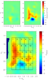 |
Fig. 4. Top left: residual map generated for a grid element showing no significant density excesses, leading to a featureless residual map; such a grid element is thus dominated by the old LMC field population. Top right: residual map for a grid element that includes the OB association LH 63. Significant density excesses can be seen across the CMD, which is due to the presence of massive OB and PMS stars. Bottom: significance map for the same LH 63 region with 25 CMD boxes overlaid; these are used to classify candidate regions based on observed density excesses (see Sect. 4). |
We use Poisson statistics to obtain the significance of any density excesses in the residual maps. If nge and ncf are the density values at a specific location in the Hess diagram for the grid element and the control field, respectively, then the density excess is simply nge − ncf; the individual statistical uncertainties are  and
and  , which gives a total uncertainty of
  for the residual. The statistical significance in the residual is thus
 (3)
(3)
This significance is computed for every point in the residual map, creating an associated significance map. Figure 4 (bottom panel) shows an example significance map. We apply the algorithm to the five grids with different radii; for every element in each grid a residual map and a significance map are obtained.
4. Identifying candidate young regions
We developed a procedure that analyses the residual and significance maps, flagging and categorising candidate regions. This was extensively tested by comparing the significance maps from grid elements containing the well-studied associations LH 60 and LH 63, and a nearby control field (Gouliermis et al. 2011). Figure 4 (top) shows residuals for the control field (left) and a grid element that contains LH 63 (right). The bottom panel shows the significance map that results from applying Eq. (3) to the LH 63 residual. It displays extended areas with significances >2 at CMD locations that are indicative of the presence of young UMS and PMS stars.
A prominent blue patch is also noticeable, suggesting a field over-subtraction, where one would expect faint main-sequence stars. This feature is likely caused by small-scale variations in the completeness that are due to crowding, which are not accurately accounted for in our method. The dark blue areas at the edge of the map are artefacts caused by the absence of stars at these CMD positions for the grid element and the corresponding control field.
We divide the colour–magnitude space into 25 boxes (Fig. 4 bottom panel), which are analysed separately. A box is flagged when the average statistical significance is higher than a predefined threshold. The threshold value is chosen to balance sensitivity to less populous associations and robustness against statistical fluctuations. To find an appropriate threshold, we analyse the distribution of the average significances in all CMD boxes across the whole tile. This distribution is approximated by a Gaussian, and the width σ describes the typical statistical fluctuation. We use either 2.5σ or 3σ as the flagging threshold (details to follow).
Depending on their properties (i.e. age and total mass), stellar populations create density excesses above the local field population in different areas of the significance maps. We analysed the residuals and significance maps for example regions with known young populations. Gouliermis et al. (2011) constructed catalogues of candidate PMS and UMS stars for LH 60 and LH 63 (age 3–5 Myr), based on a statistical analysis of HST photometry in the F555W and F814W filters. After correcting for a systematic difference of 0.42″ in RA, we cross-correlated the HST and VMC catalogues with a conservative 0.3″ matching radius. We further compared the magnitudes of the matched pairs in the VISTA Y filter and in the HST F814W filter. The transmission curves of these filters are similar enough for these magnitudes to be comparable. For the matched pairs (F814W − Y) is on average 0.43 mag, with a dispersion of 0.86 mag. To select a clean sample, pairs with (F814W − Y) ≥ 2 mag were excluded.
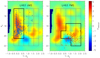 |
Fig. 5. Same significance map in the background as shown in Fig. 4 (bottom). Blue and red symbols display VMC sources that are successfully matched to the LH 63 UMS (left) and PMS (right) catalogues from Gouliermis et al. (2011). Thick black lines highlight the boxes relevant for the UMS and PMS classifications, respectively (see also Fig. 6). |
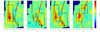 |
Fig. 6. From left to right: significance maps for grid elements classified as UMS-only, PMS-only, UMS+PMS, and “old”. The CMD boxes relevant for each classification are highlighted. Boxes that are flagged in the particular significance map are numbered. PARSEC isochrones (Bressan et al. 2012) are shown in all panels. Red isochrones represent ages from log(t/yr) = 9.6 − 9.8, with a metallicity of Z = 0.0033 (Tatton et al. 2013); they show the typical location of the old LMC field population. Black isochrones represent young populations from log(t/yr) = 6.0 − 6.8 (Z = 0.008; Rubele et al. 2012). The two black isochrones in the rightmost panel represent populations of log(t/yr) = 8.5 − 8.6 (Z = 0.008). All isochrones are reddened according to the mean extinction for that particular grid element (Sect. 3.2). In the second panel the theoretical positions for stars of three different masses are shown (colour-coded circles) for the youngest and oldest black isochrones. |
In LH 60 we found 112 and 174 VMC counterparts to the HST PMS and the UMS sources, respectively. For LH 63 the corresponding numbers are 125 and 2693. Figure 5 shows the VMC counterparts for the LH 63 UMS and PMS catalogues, with the significance map shown in the background. A clear gap is visible between the two populations, since the HST catalogue excludes areas in the optical CMD that are heavily contaminated by field stars. Clearly, the UMS matches coincide very well with areas of statistically significant density excesses; the highlighted CMD boxes (Fig. 5 left) cover the majority of UMS matches and the corresponding density excesses. Overall, 237 out of 269 UMS matches are located within these eight boxes; some matches are located near the red giant branch and are likely contaminants in the UMS catalogue (Gouliermis et al. 2011).
The situation is more complicated for the PMS matches. Some matches fall on the strong negative density excess described previously; we did not use this part of the CMD to identify PMS populations precisely to avoid severe contamination by main-sequence stars. The large scatter in the CMD distribution of the PMS matches can be due to photometric errors and/or young stellar variability (e.g. T Tauri stars or FU Orionis variables; Contreras Peña et al. 2014; Rice et al. 2015). In addition, the PMS population could have either an age spread, or it could consist of multiple populations with different ages, similar to what has been seen in Orion (Beccari et al. 2017). Nevertheless, the regions with the most significant density excesses suggest a PMS distribution that is brighter than the distribution of HST-matched stars. Two effects likely contribute to this. Firstly, small-scale completeness variations can be significant in crowded regions like LH 63 (see Sect. 3.3). This can lead to over-subtraction during the control field decontamination process, which eliminates a potential density excess due to faint PMS stars. Secondly, the HST PMS catalogue included mostly relatively faint PMS stars (F814W ≥ 21.2 mag). The density excess seen in our maps includes brighter PMS candidates excluded from HST optical catalogues. Using the location of the PMS matches and the location of the typical density excesses seen in the residual maps of known young associations, we selected the CMD boxes highlighted in the right panel of Fig. 5 as PMS indicators. Ninety-six out of 125 PMS matches are within this area, and overall, around 85 % of the HST–VMC counterparts are located within the outlined UMS and PMS boxes.
Using these contiguous regions in the CMD that are indicative of the presence of specific populations, we classify each grid element based on which boxes are flagged in its significance map. Four classifications are adopted:
UMS-only. At least two adjacent boxes are flagged in the UMS CMD region. Figure 6 (left) shows a typical example of this classification. It covers a broad age range from ∼10 to ∼300 Myr. Based on artificial cluster tests (see Sect. 5.1), a minimum cluster mass of ∼500 M⊙ is needed to reliably flag two UMS boxes. For populations younger than 10 Myr, the PMS population is also detectable, changing its classification to UMS+PMS (see below). Beyond ∼300 Myr, sufficiently massive clusters (>1000 M⊙) create a significant red giant excess, which will trigger the classification “old”.
PMS-only. At least two adjacent boxes are flagged in the PMS CMD region (second panel in Fig. 6). This classification traces young (<10 Myr), low-mass clusters and associations up to around ∼500 M⊙. While the PMS phase for stars with masses ≲0.5 M⊙ can last up to 100 Myr (e.g. Tout et al. 1999), PMS populations older than ∼10 Myr are too faint to be detected in the VMC survey. Young clusters and associations with masses above 500 M⊙ also flag boxes typical of UMS populations, changing the classification to UMS+PMS.
UMS+PMS. A grid element is classified as UMS+PMS if a total of at least three boxes in both the typical PMS and UMS CMD regions are flagged. Adjacency is not strictly enforced, since a minimum of three flagged boxes always leads to reasonable combinations. The same age range as in the PMS classification is probed (<10 Myr), but the clusters and associations are more massive, since enough massive stars need to be present to flag UMS boxes. Examples for this classification are shown in Fig. 6 (third panel) and Fig. 4.
Old. This classification requires a minimum of three flagged boxes in the red giant branch and the fainter parts of the UMS CMD region. The flagging threshold for the red giant branch boxes is 2.5σ (compared to 3σ for the other boxes). We found in tests with synthetic and real clusters that this threshold reduction improves our ability to classify old clusters, without a noticeable increase in the number of false positives. Grid elements with clusters older than ∼300 Myr and more massive than ∼1000 M⊙ fall into this classification (Fig. 6, right).
5. Testing the identification strategy
5.1. Synthetic clusters
To assess the sensitivity of this procedure to young populations of different masses and ages, we ran tests using synthetic clusters. To generate the synthetic clusters, we used the Popstar Evolutionary Synthesis Code (Mollá et al. 2009) and adopted a Kroupa IMF (Kroupa 2001, 2002). There is no conclusive evidence that the IMF in the LMC is significantly different from the Galactic IMF (for M > 1 M⊙; Gruendl & Chu 2009; Liu et al. 2009a,b), with the possible exception of 30 Doradus (Schneider et al. 2018b). NIR photometry for the VISTA filter set was obtained using PARSEC models (Bressan et al. 2012). Synthetic clusters were generated for the following mass and age combinations:
Mcl ∈ [250 M⊙, 500 M⊙, 1000 M⊙, 2000 M⊙, 3000 M⊙]
log(t/yr) ∈ [6.0, 6.3, 6.7, 7.0, 7.5, 8.0, 8.5, 9.0].
The cluster masses are representative of LMC clusters within this age range (de Grijs & Anders 2006). We also adopted the canonical LMC metallicity of Z = 0.008. For every mass–age combination, ten clusters were created. Incompleteness was applied and photometric errors added to match the quality of the VMC data before injecting the clusters into the PSF tile catalogue. All clusters were seeded in control-field-like grid-elements with flat significance maps. Each synthetic cluster was fully contained within a grid element, a reasonable assumption given that even the smallest elements have a physical radius of 10 pc (1 pc ≅ 4″ at the LMC distance). The enhanced PSF tile catalogues for every synthetic cluster were ingested into our algorithm, and the resulting residuals and significance maps were evaluated. If a synthetic cluster was classified into one of the four classes defined in Sect. 4 and in agreement with the cluster input properties, it is considered to be reliably identified.
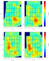 |
Fig. 7. Top: significance map for a PMS-only classified grid element (left) is compared to a synthetic stellar population of 250 M⊙ and 1 Myr (right). Bottom: similar to the top, but showing a UMS+PMS classified grid element (left) and a synthetic stellar population of 1000 M⊙ and 5 Myr (right). Flagged boxes are numbered in each map. |
In Fig. 7 we show examples of significance maps generated from observed data, compared with maps generated from synthetic clusters. The top left panel shows a PMS-only classified element with a clear PMS signal and no UMS excess. This suggests the presence of a very young, low-mass population. A synthetic population of 250 M⊙ with an age of 1 Myr generates a very similar significance map. The bottom left panel contains the significance map for a UMS+PMS classified element. A synthetic stellar population of 1000 M⊙ with an age of 5 Myr creates a similar significance map. Since at 5 Myr many PMS stars fall below the sensitivity limit, the PMS signature is relatively weak.
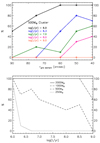 |
Fig. 8. Top panel: detection percentages for 500 M⊙ clusters of different ages for grid-element radii from 90″ to 40″. A general increase in detection rates with decreasing radius is noticeable. A decrease in detection rates with increasing cluster age is evident as well. Bottom panel: detection percentages for clusters of four different masses across the age range from 1 Myr to 1 Gyr for the 40″ radius. A decrease in sensitivity for older ages and lower masses is apparent. Clusters more massive than 500 M⊙ show high detection rates for young ages. |
Figure 8 shows the results of our synthetic cluster tests. In the top panel the detection rates for the different grid element radii for 500 M⊙ clusters of various ages are presented. While for the 90″ radius clusters of this mass are rarely detected, the percentages increase steadily for smaller radii. At a radius of 40″ the detection rates are at least 60% for ages where one would expect to find PMS stars. The bottom panel shows the results obtained using the 40″ grid for four different cluster masses in more detail. For masses ≥1000 M⊙, clusters are always detected, with a drop in detection rate only noticeable at 1 Gyr. For lower masses, the detection rate drops steadily with age. This is due to a decrease of flagged UMS boxes with increasing age, as more massive stars evolve away from the main sequence onto the red giant branch. At these cluster masses, this does not necessarily trigger the flagging of boxes that lead to the “old” classification. For ages ≲ 10 Myr, the majority of 500 M⊙ clusters are detected. Even though the detection rate drops sharply for masses <500 M⊙, it remains high for very young ages.
These tests reveal three clear trends. Rather obviously, the more massive a synthetic cluster at any given age, the higher the probability of a reliable detection. Secondly, with smaller grid element radius, the probability of detection for a given synthetic cluster mass and age increases. The reason is that the same number of synthetic stars cause a higher density excess in the residuals of smaller grid elements, leading to a higher flagging probability. Thirdly, the detection rates generally decrease with age. The luminosity of intermediate- and low-mass PMS stars decreases as they approach the main sequence. Hence, an increasing fraction of PMS stars falls below the sensitivity limit of the VMC survey for progressively older ages.
Most likely classifications for mass and age ranges based on synthetic cluster tests.
Table 1 presents an overview of the most common classifications for synthetic clusters of different age and mass ranges. The decrease of detectable PMS stars with age causes an increase in the minimum cluster mass that is necessary to detect a PMS signature. Beyond 10 Myr, the VMC survey is not sufficiently deep to reliably detect any remaining PMS stars. Therefore, all detected clusters are classified either as UMS-only or as “old”. The tests reveal that massive (≳2000 M⊙) clusters within the age range 30 Myr–1 Gyr can be mis-classified as UMS+PMS, and thus contaminate the UMS+PMS class. However, the level of contamination is 2.5% at most.
In summary, we conclude that for a given mass, a cluster or association is easier to detect and classify at a young age (preferably <10 Myr); this is mostly due to the sensitivity and completeness limits of the VMC survey. While ∼28% of detected clusters with age 10 Myr have a PMS signature leading to a PMS-only or UMS+PMS classification, this fraction increases to ∼66% for 5 Myr-old populations and ∼98% for very young ages (≤ 2 Myr). More massive clusters are obviously more likely to be identified. Another important result is that finer grids are better suited to finding low-mass clusters, despite the effects of small number statistics due to the decreasing number of stars per grid element.
5.2. Literature clusters
The synthetic cluster tests provided valuable results about the mass and age ranges that are effectively traced with our method. However, as these synthetic clusters were only injected into the PSF catalogue rather than into the images, information on the sensitivity to different cluster radii and star count density profiles is lacking. We compiled a list of 31 clusters and associations from the literature (Gouliermis et al. 2003; Glatt et al. 2010; Popescu et al. 2012). Our list is not a complete census of clusters in the pilot field, but provides a reliable sample of clusters with different ages and sizes. The selected systems span an age range from a few Myr up to around 1 Gyr, and apparent sizes from 10″ to over 100″ (sizes were estimated visually from the VMC images).
Table 2 shows how many clusters are classified as a function of grid element radius. With decreasing grid element size, the number of unclassified clusters decreases monotonically. This trend is in line with the results from the synthetic cluster tests, where an increasing sensitivity for the finer grids was observed. For the finest grid, 25 out of 31 literature clusters are classified with our method. For 23 of these, their classifications and inferred broad age range (see Table 1) are consistent with published literature ages. The two remaining clusters have literature ages of log(t/yr) ∼ 7.8; since an RC signature is detected, our method classifies these clusters as old, implying an age ≳300 Myr.
Number of classified clusters from the sample of 31 clusters from the literature as a function of grid element radius.
Six unclassified clusters remain, four of which flag a single CMD box. Since this does not trigger a classification, these four clusters are at the sensitivity limit of the 40″ grid. The unclassified clusters are either spatially small compared with the grid element and/or are relatively old (based on their literature ages). Two of the six unclassified clusters are the smallest in our list with radii of 10″ and 14″, ∼6% and ∼12% of a grid element area. This indicates that our method is mostly sensitive to clusters with r ≳ 3 pc at the LMC distance. For four of the six unclassified clusters, the literature age is in the range 7.3 ≲ log(t/yr) ≲ 8.7. The stellar populations of old clusters move towards areas in the CMD that are more heavily contaminated by the old field population, further decreasing the sensitivity. This confirms the results from the synthetic cluster tests that comparatively old systems have lower detection rates. Given that our stated goal is to identify young populations, a decrease of detection rate with cluster age is not an issue.
5.3. Final choice of grid element radius
Our analysis clearly advocates the use of the 40″ radius grid because of its increased sensitivity. A further decrease in radius leads to grid elements without any RC stars, impairing the ability of the method to correct for reddening differences between a grid element and its control field. On average, a 40″ grid element is populated by 265 stars, with 171 stars being the minimum. Our subsequent analysis focuses on the optimal 40″ radius grid.
6. Results
Applying our method to the PSF catalogue from the pilot field provides the residual and significance maps, flagged boxes, and classification for every grid element. For the 40″ grid, 10,730 grid elements are unclassified, 298 are classified as UMS-only, 84 as PMS-only, 124 as UMS+PMS, and finally, 14 are classified as “old”.
6.1. Spatial distribution of the young populations
6.1.1. Global properties
Figure 9 shows the spatial distribution of the 208 grid elements with a significant PMS contribution (classified as UMS+PMS and PMS-only, cyan and yellow crosses, respectively). These grid elements are not distributed uniformly, but instead concentrate in areas with enhanced dust emission as traced by Spitzer in the IRAC 8.0 μm band (Meixner et al. 2006). Around 80% of them are found in three main regions: N 44, N 51, and N 148 (see Fig. C.1 for a detailed view). N 44 and N 51 are well-studied large star formation complexes (e.g. Carlson et al. 2012). Almost all classified elements associated with these complexes are located within regions of about 290 arcmin2 (∼65 200 pc2) and 380 arcmin2 (∼85 500 pc2). On these spatial scales, star formation complexes contain young populations formed in multiple and/or extended star formation events (see Gouliermis 2018, for a detailed review). For comparison, the HTTP survey of the 30 Doradus region covers ∼168 arcmin2 (Sabbi et al. 2013), within which Schneider et al. (2018a) found evidence for complex spatial and temporal substructure amongst the massive stars. Towards the south-eastern corner of the field lies another concentration of classified elements associated with N 148, which is also prominent in CO (Wong et al. 2011) and dust emission (Meixner et al. 2006). A fourth group is situated to the north-east (labelled Region A). While the numbers of PMS-only and UMS+PMS classified grid elements are small, this region exhibits the highest concentration of UMS-only classified elements (see Appendix A), indicating a comparatively mature population. Another concentration of classified elements is associated with the emission nebula N 138. A more detailed discussion of these individual regions is found in Sect. 6.1.2.
 |
Fig. 9. Top left: three-colour composite image with VMC Y (blue) and Ks bands (green), and Spitzer IRAC 8.0 μm (red). The rectangle shows the region covered by our analysis. Small crosses mark the centres of grid elements for the 40″ grid that are classified as PMS-only (yellow) or UMS+PMS (cyan). Several prominent regions are highlighted and labelled (spatial sizes according to Bica et al. 2008) and discussed further in Sect. 6. Top right: inverted grey-scale map of Hα emission (Smith et al. 2005). Bottom: PMS density contours for elements classified as PMS-only or UMS+PMS derived from the residual maps of the grid elements. The outermost contour represents ΔnPMS = 2.4 stars arcmin−2 (see Sect. 6.2 for details); every subsequent contour represents an increase in density by 3 × ΔnPMS. |
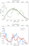 |
Fig. 10. Top: normalised distance distribution for all possible grid pairs for the 208 PMS-only and UMS+PMS classified elements (green line), and for a same-size sample of randomly distributed unclassified elements (black line). Bottom: same as the top panel, but separating the two classifications. |
Outside these complexes, classified grid elements are fairly scattered; Fig. 9 shows 12 isolated elements with signatures of a young population. An inspection of the residuals and significance maps for these isolated elements shows that they are generally consistent with the maps from elements located within star-forming complexes and from the synthetic clusters. A comprehensive analysis of the stellar populations of these isolated elements is beyond the scope of this paper.
Overall, UMS+PMS classified grid elements are almost exclusively found in groups. PMS-only grid elements, on the other hand, are often located on the outskirts of populous UMS+PMS star groups or appear isolated. To quantify the degree of clustering, we calculated the distance between every possible pair of classified elements. Figure 10 (top) shows this distance distribution, together with a distribution for a same-size sample of randomly placed unclassified elements. To eliminate statistical fluctuations, we ran this simulation 100 times and used the mean and standard deviation values to construct the random distribution histogram with corresponding uncertainties. Because of the finite pilot field size, the number of possible random pairs decreases for large distances. For small distances (<180 pc), the observed distribution shows a clear excess of classified pairs as a consequence of the clustered distribution of young stars. The broad peak between 450 pc and 700 pc is due to the distances between N51 and N44, and between N51 and Region A. The peak between 900 pc and 1050 pc is caused by the distances between N44 and N 148, N44 and Region A, and N51 and N 148.
Figure 10 (bottom) displays the distance distribution for the PMS-only and UMS+PMS subsamples separately. They are distinct and not simply scaled-down from the overall distribution. As a result of the very strong clustering of the UMS+PMS classified elements, the corresponding distribution shows very prominent peaks. The very narrow peak between ∼130 pc and ∼170 pc is due to the distances between associations within N44 and N51. The broad peak for distances ≲200 pc suggests a similar distribution of UMS structure sizes, as seen in other star formation complexes in the LMC (Sun et al. 2017b,a) and in the SMC (Sun et al. 2018).
In contrast, the PMS-only distribution shows smaller variations, in agreement with a more extended spatial distribution. It is a common observation in young clusters that high-mass stars are more centrally located than intermediate- and low-mass stars (e.g. Zinnecker et al. 1993; Gennaro et al. 2011; Pang et al. 2013). The underlying physical process is assumed to be dynamical mass segregation (e.g. Bonnell & Davies 1998; Allison et al. 2009). Such effects are relevant within individual clusters, which are usually smaller than one element in our grid. However, since segregation timescales are of the order of several crossing times (e.g. de Grijs et al. 2002), dynamical mass segregation is too slow to explain the observed spatial distribution on the scales of the complexes N44 and N51.
In agreement with our results, the HTTP survey found that for the 30 Doradus region, the UMS stars also mostly concentrate in a few main population centres (Sabbi et al. 2016), while the PMS stellar distribution displays a larger spatial dispersion (Cignoni et al. 2015). Based on the distribution of PMS stars and the location of ionised filaments in 30 Doradus, Sabbi et al. (2016) find evidence of constructive feedback from massive stars igniting the birth of new generations of stars. In N44, Chen et al. (2009) also reported evidence of triggered star formation. Triggering by massive stars could operate on larger spatial scales than mass segregation; it is thus a viable scenario for the different spatial distribution between PMS-only and UMS+PMS elements, since it could lead to the formation of less massive clusters or associations in the outskirts. This is observed in the Carina Nebula, where the currently ongoing star formation seems to produce only stars up to ∼10 M⊙ (Gaczkowski et al. 2013).
Alternatively, the evaporation of bound clusters due to gas expulsion could also result in the observed spatial distribution of classified elements. After a quick gas removal phase (≲1 Myr), clusters are predicted to expand to half-mass radii ≳10 pc (for masses ∼5000 M⊙) within 10 Myr (Pfalzner et al. 2014). Crucially, they develop an extended stellar halo of ejected stars that can extend beyond 100 pc (Moeckel & Bate 2010). In the comparatively low stellar density environment of such halos, there will naturally be fewer UMS stars, thus increasing the likelihood of PMS-only classified elements in the cluster outskirts.
6.1.2. Individual regions
Several regions, associated with a large number of classified elements, are identified in Fig. 9. As described before, in N 51 and N 44, the UMS+PMS-classified elements are strongly clustered, whilst the PMS-only elements are often located in the outskirts of these regions. In both complexes significant dust and Hα emission is also observed. In N 44, Hα emission and the UMS+PMS-classified elements are spatially coincident, as would be expected since the ionising radiation from the UMS stars is the origin of the Hα emission. Two large substructures can be seen: the larger substructure near the centre corresponds to the associations LH 47 and LH 48, and the smaller substructure towards the south includes LH 49. To the east of N 51, a similarly strong overlap between Hα emission and classified elements is seen. To the west, the intense Hα emission traces a bubble-like shape, but the overlap with classified elements is patchy. Two OB associations, LH 51 and LH 54, are associated with this bubble (e.g. Book et al. 2009).
In addition to these complexes, the two most prominent concentrations of classified elements are located in the western part of N 148 and in Region A. N 148 is an intense and vigorous star-forming region (e.g. Ambrocio-Cruz et al. 2016) and is only partially covered by our analysis. Most grid elements are classified as PMS-only without a significant UMS population; this suggests the existence of a distributed population of intermediate- and low-mass PMS stars associated with N 148, identified here for the first time. Based on comparisons of the significance maps with synthetic clusters, some of the PMS-only grid elements seem very young (∼1 Myr). The presence of significant dust and CO emission combined with the lack of extended Hα emission provides further evidence of a young population devoid of UMS stars.
The classified elements in Region A combine relatively weak PMS signatures with strong UMS signatures, suggesting an older age. The most prominent cluster in this area, NGC 2004, indeed has an age of ∼20 Myr (Niederhofer et al. 2015), resulting in a PMS population that is too faint to be reliably detected with the VMC data. Region A also lies in an area with no significant dust or Hα emission. This all hints at a comparatively old age of the dominant populations in the region, probably a result of the energetic feedback from massive stars that have significantly eroded the interstellar medium.
Another grouping of classified elements is found to the north-east of the emission nebula N 138. More specifically, the PMS-only and UMS+PMS-classified regions are spatially coincident with the H II regions N 138A and N 138C. In N 138A Indebetouw et al. (2004) found an ultracompact H II source, indicative of very young massive stars.
Our method for classifying young populations not only identifies all major star-forming complexes in tile LMC 7_5, but also exposes their full extents and distribution for the first time.
6.2. Quantitative analysis of the PMS populations
Using the residual maps, we calculate the number density of PMS candidates as well as the overall number of PMS candidates in the classified elements. Taking the mean density excess of the flagged boxes relevant for PMS populations (see Fig. 6) and multiplying it by the area covered by these boxes in the CMD, we derive the PMS number density. We obtain a mean PMS number density nPMS =12.7 stars arcmin−2 over all elements classified as PMS-only or UMS+PMS. The uncertainty, estimated by analysing the density fluctuations in the residuals of non-classified elements, is ΔnPMS = 2.4 stars arcmin−2. Multiplying the PMS density by the solid angle of the grid element (∼1.4 arcmin2), we derive the number of PMS candidates (NPMS). On average, there are NPMS = 17.7 ± 3.4 per classified element.
In Fig. 9 we plot the PMS density contours. The highest density (40 stars arcmin−2≅ 0.18 stars pc−2) is found within N 44. Large complexes contain multiple high-density peaks, displaying a hierarchical structure similar to that found for UMS stars by Sun et al. (2017a,b). Integrating over all classified elements and accounting for the overlap between neighbouring grid elements, we determine a total number of PMS candidates of 2256 ± 54. This result is a lower limit because the incompleteness in the VMC data at magnitudes typical of PMS stars is significant.
Number of PMS candidates in the whole LMC 7_5 tile and individual prominent regions.
Table 3 lists the number of PMS candidates for the whole pilot field as well as for the five regions described in the previous sections. Overall, ∼80% of all PMS candidates identified are located in one of these regions, with N 44 being the most populous.
For comparison, Meingast et al. (2016) estimated the entire young stellar population of the Orion A molecular cloud to have between 2300 and 3000 stars. Using a Kroupa IMF, this gives 300–390 stars with masses 1 M⊙ ≤ M* ≤ 4 M⊙, which is the PMS mass range our method is sensitive to (see Fig. 6). The area covered by the Orion survey (18.3 deg2) corresponds to 4.5 arcmin2 or 3.2 grid elements at the LMC distance. In the Carina Nebula complex, 8781 young stars were identified based on their NIR colour excess (Zeidler et al. 2016). Applying a Kroupa IMF to the same mass range gives ∼1150 stars that could potentially be identified as PMS with our method. This is comparable with our PMS count for the N 44 complex. We note, however, that this estimate includes only sources with an NIR colour excess. At the LMC distance, the area observed in Zeidler et al. (2016) corresponds to 51.5 arcmin2 or around 37 grid elements, which is approximately the area covered by the large group of classified elements in the centre of N 44. Incompleteness and crowding would obviously reduce the number of PMS sources we would be able to detect.
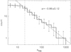 |
Fig. 11. Cumulative number distribution for the 31 PMS structures (0.2 dex bins). The vertical dashed line indicates the sensitivity limit, while the dash-dotted line represents a power law with a slope of −0.86. The error bars represent the Poissonian uncertainties. |
To obtain a more detailed view of the morphology of the PMS populations, we define PMS structures as regions enclosed by the lowest density contour in Fig. 9. We detect 31 structures in total, the most populous of which is located in N 44 and contains ∼670 PMS candidates. Figure 11 shows the cumulative NPMS distribution for the PMS structures.
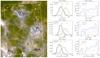 |
Fig. 12. Left panel: three-colour composite image with Spitzer MIPS 70 μm in blue, Herschel PACS 160 μm in green, and Herschel SPIRE 350 μm in red; the density contours are the same as those in Fig. 9. Middle panels: dust emission distribution for image pixels in areas covered by the UMS+PMS and PMS-only classified elements, and by the same number of randomly selected unclassified elements. A Gaussian fit is plotted and the mean of the fit is indicated. Right panels: dust emission vs. young stars number density for the PMS and UMS+PMS classified elements. The error bars show the typical standard deviations within the dust emission bins. |
For NPMS > 20 the distribution can be approximated by a power law with a slope α(NPMS) = −0.86 ± 0.12. Studies of cluster mass distributions have shown that high-mass clusters are less numerous than low-mass ones (e.g. Zhang & Fall 1999; Hunter et al. 2003; de Grijs & Goodwin 2008), with a slope α(M) ∼ −1. In a histogram using equal logM intervals, α(M) = −1 is equivalent to a mass distribution function n(M)dm ∝ M−βdm with δ = −2, which is the slope expected for a scale-free hierarchical star formation scenario governed by turbulence (e.g. Fleck 1996; Elmegreen 2008). Converting NPMS obtained from our method into structure masses would yield very uncertain estimates because of the significant age dependence of the sensitivity limit of our VMC-based method (see Sect. 5.1). For predominantly “old” PMS populations, α(M) > α(NPMS) is expected, since a large fraction of PMS structures will have low PMS counts; for predominantly young PMS populations, we could expect α(M) < α(NPMS). A more thorough discussion of the mass distribution should take the ages of the populations into account.
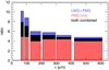 |
Fig. 13. Ratios of the mean dust emission observed for classified elements and the field average. The widths of the bars mimic the filter bandwidths. |
6.3. Comparison with dust emission maps
Since dust emission should be proportional to the product of dust mass and input stellar radiation (because of the energy balance between absorption and emission), one would expect a strong correlation between the number of young stars and dust emission. Bright FIR emission is usually associated with high star formation rates (see Casey et al. 2014 for a comprehensive overview); it originates from the radiation of the young stars that is processed by dust from the remnants of their natal molecular clouds and re-emitted at longer wavelengths. Skibba et al. (2012) have reported that some regions with bright dust emission in the MCs coincide with known star-forming regions. Moreover, in M 33 only young structures (<100 Myr) were found to correlate with FIR surface brightness (Javadi et al. 2017). Given that the presence of PMS stars is an indicator of recent star formation, we examined the relation with FIR emission in regions covered by the UMS+PMS and PMS-only classified elements.
We made use of data from the SAGE and HERITAGE surveys in six FIR bands ranging from 70 to 500 μm (Meixner et al. 2006, 2013). Figure 12 (left) shows the PMS density contours overplotted onto an RGB image (70, 160 and 350 μm) of the pilot field. PMS-only and UMS+PMS-classified elements are located along ridges and filamentary structures with bright dust emission. The only significant exceptions are Region A and some isolated PMS-only elements. As mentioned previously, the weak dust emission for Region A is in agreement with the inferred comparatively old age of the stellar populations.
The concentration of elements with PMS populations in regions with bright dust emission is explicitly shown in the middle histograms of Fig. 12. The dust emission distributions for grid elements associated with PMS populations and a randomly selected sample of unclassified elements are clearly distinct; in particular, the strongest observed emission is always associated with young stellar populations.
Figure 12 (right) shows the dust emission versus the average number density of young stars for the same three FIR bands, separating PMS-only and UMS+PMS-classified grid elements. We computed UMS densities for the UMS+PMS elements similarly to the PMS densities (Sect. 6.2) to obtain the total density of young stars. We calculated the mean FIR emission for every classified element and grouped them in 0.2 dex bins; for every bin, the average number density of young stars was determined. For the UMS+PMS elements, we observe a relatively weak but consistent trend towards higher stellar number densities with increasing dust emission for all wavelengths. Hony et al. (2015) found a positive correlation between the number density of young stars (UMS and PMS stars identified using HST photometry (Gouliermis et al. 2006b)) and dust surface density in the prominent star-forming complex NGC 346 in the SMC. Their analysis, on scales comparable to the size of our grid elements, is in agreement with the trend in Fig. 12 (right). For PMS-only elements, however, we do not observe an increase in stellar density with dust emission; less clustered low- and intermediate-mass PMS populations are likely more affected by the limitations of the VMC data.
Depending on the wavelength, the emission associated with the UMS+PMS and PMS-only classified elements is between four and eight times brighter than the field average (Fig. 13); the strongest enhancement is found for the shorter wavelengths. Furthermore, the ratios for the PMS-only sample (red) are essentially independent of the wavelength, while the ratio for the UMS+PMS sample (blue) increases significantly towards shorter wavelengths. This is evidence that the dust is heated primarily by the young massive UMS stars, while the PMS populations contribute very little. This is consistent with studies that found that warm dust follows the distribution of massive stars in the LMC (Bernard et al. 2008), as well as in Galactic star-forming complexes (Preibisch et al. 2012; Roccatagliata et al. 2013). As a comparison, for the UMS-only classified elements (not shown), the dust emission is between 1.3 and 1.8 times higher than the pilot field average. The analysis in this section confirms the important role that young UMS stars play in heating the dust.
7. Summary and conclusions
We presented a method for identifying PMS populations (≥1 M⊙) using data from the VMC survey. The method applies a Hess diagram analysis in the Ks/(Y − Ks) space, including corrections for reddening and completeness, to distinguish young stellar populations from the underlying field; this analysis is performed independently on individual fixed-size spatial grid elements. Young populations are identified as density excesses (with respect to the field population) in pre-defined regions of the differential Hess diagrams. Depending on the location of these density excesses with respect to theoretical expectations (i.e. isochrones), we classify the population within a grid element into one of the four classes: PMS-only (population of young low-mass stars), UMS+PMS (young population with well-sampled IMF across the mass range), UMS-only (predominantly older population dominated by a prominent main-sequence population), and “old” (population that displays a significant contribution from evolved stars, in particular populating the red giant branch).
We applied our method to a ∼1.5 deg2 VMC pilot field (LMC 7_5) and summarise our findings below.
Tests with synthetic clusters explore the sensitivity of the method in the age range 1 Myr–1 Gyr and the mass range 250 M⊙–3000 M⊙. We find that PMS populations can be identified up to an age of ∼10 Myr for cluster masses > 1000 M⊙. Beyond 10 Myr, any remaining PMS populations are below the VMC sensitivity limit. The sensitivity increases towards younger ages: PMS populations with ages ≤ 2 Myr can be detected for clusters with masses down to 250 M⊙.
We detected a total number of 2256± 54 PMS stars in the pilot field. The most populous region is the N 44 complex, which has 1000± 38 PMS stars. This estimate must be taken as a lower limit because the VMC data are incomplete and our method has a sensitivity limit.
The spatial distribution of elements with PMS populations is clearly inhomogeneous and clustered. UMS+PMS elements are almost exclusively found in large groups, while the PMS-only elements are more dispersed and often located in the outskirts of large star-forming complexes.
Large star-forming complexes consist of multiple high stellar density peaks, with the highest densities found in the N 44 complex. Overall, we detect 31 PMS structures whose number distribution can be approximated by a power law with a slope of −0.86± 0.12. A mass distribution with this slope would be broadly consistent with a hierarchical star formation scenario governed by turbulence.
The PMS populations are mostly located along ridges with intense dust emission in the FIR (70–500 μm). We observe a correlation between the dust emission and the number of young stars for the UMS+PMS elements. This is not the case for the PMS-only elements that lack UMS stars. Dust emission is around four to eight times brighter for the UMS+PMS elements than in quiescent regions; at the shortest wavelengths, the emission can be as much as ten times brighter. This is likely due to dust heating by the radiation from the young UMS stars.
Our analysis recovers all known star formation complexes in this field, and for the first time reveals their true spatial extent.
In the south-eastern corner of LMC 7_5, we discovered a significant intermediate- and low-mass PMS population that is likely associated with the wider N 148 star-forming complex. Comparison with synthetic cluster Hess CMDs suggests a very young age (∼1 Myr) for this population. This population is co-spatial with significant CO emission.
Our method clearly shows the potential of the VMC survey to identify and characterise intermediate- and low-mass young stellar populations on the scale of the whole Magellanic system. We are working on applying our method to other LMC and SMC VMC tiles.
Acknowledgments
This work is based on observations obtained with VISTA under ESO-program ID 179.B-2003. We thank the Cambridge Astronomy Survey Unit (CASU) and the Wide Field Astronomy Unit (WFAU) in Edinburgh for providing calibrated data products through the support of the Science and Technology Facility Council (STFC). This research has made use of the SIMBAD database, operated at CDS, Strasbourg, France, and of the NASA Astrophysics Data System (ADS) bibliographic services. We thank Marta Sewilo for sharing her extensive compilation of LMC images and catalogues. Viktor Zivkov acknowledges studentships from ESO and the Faculty of Natural Sciences, Keele University, UK. We thank the anonymous referee for the constructive comments.
PAdova and TRieste Stellar Evolution Code http://stev.oapd.inaf.it/cgi-bin/cmd_2.7
Based on a catalogue matching with shifted coordinates, we estimate that ∼3% of the UMS matches and ∼10% of the PMS matches are spurious.
Appendix A: Spatial distribution of the older population
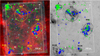 |
Fig. A.1. Left: three-colour composite image with VMC Y (blue) and Ks bands (green), and Spitzer IRAC 8.0 μm (see also Fig. 9). Green and white crosses mark the locations of elements classified as UMS and “old”, respectively. The UMS+PMS and PMS-only classified elements are included as blue circles to facilitate comparison. Right: same as the left panel, but using an inverted grey-scale image of the Hα emission. |
In Sect. 6.1 we analysed the spatial distribution of elements showing a PMS signature. We found especially pronounced clustering for UMS+PMS-classified grid elements, which represent young and relatively massive populations. Here we investigate the spatial distribution of the 298 grid elements classified as UMS-only. They contain comparatively old populations (10–300 Myr; see Sect. 4).
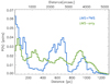 |
Fig. A.2. Normalised distance distribution for all possible grid element pairs classified as UMS+PMS (blue) and UMS-only (green; see also Fig. 10). |
Figure A.1 shows the location of the grid elements classified as UMS-only and “old”. Their spatial distribution is morescattered across the pilot field than the UMS+PMS elements. Consequently, more UMS-only elements are either isolated or located in small groups outside the known complexes. The concentration of UMS-only elements in region A is noticeable and is further confirmation of the comparatively older age of this population. The 14 grid elements classified as “old” are scattered across the field and are neither co-spatial with young grid elements, nor with any significant dust or Hα emission. Twelve of them seem associated with known LMC clusters (Bica et al. 2008).
Figure A.2 is equivalent to Fig. 10 (bottom), but shows the distance distributions for all possible pairs of UMS+PMS and UMS-only classified elements. Some clustering is present for UMS-only elements, but it is much less pronounced than that for the UMS+PMS classified elements; UMS-only elements show a comparatively smooth distribution. This is in agreement with the temporal evolution of young stellar structures, which are observed to disperse on long timescales (e.g. Sun et al. 2017a).
Appendix B: Reddening correction
Before comparing a grid element with its corresponding control field, we redden the control field according to the distribution of RC stars in the grid element (see Sect. 3.3). Figure B.1 shows how this correction is performed. The blue line represents the cumulative colour distribution of RC stars in the control field. Since the control field combines several grid elements, it contains many RC stars. This creates a very smooth distribution. The steep slope indicates a compact RC with little differential reddening. The black line shows the cumulative distribution for the grid element being studied. Its slope is shallower because the RC is more spread out. Especially the top ∼25% of the most strongly reddened stars suggests substantial differential reddening.
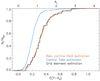 |
Fig. B.1. Cumulative colour distribution of RC stars for the grid element under investigation (black line), and for the corresponding control field before and after the reddening correction (blue and red lines, respectively). RC stars are defined by the RC selection box in Fig. 3. The intrinsic RC colour adopted is (Y − Ks)0 = 0.84 mag (Tatton et al. 2013). |
After the reddening correction is applied to the control field population, its RC distribution (red line) closely follows the grid element RC distribution. Differential reddening is accounted for, which would not have been possible by simply adopting a fixed reddening value for the control field stars.
Appendix C: Images of selected star-forming complexes
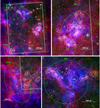 |
Fig. C.1. Three-colour composite image (top left) of the analysed area with Hα emission in blue, Ks (2.15 μm) in green, and Spitzer IRAC 8 μm in red. Regions and contours are the same as in Fig. 9. Other panels show enlarged views of selected star-forming complexes: N 44 (top right), N 148 (bottom left), and N 51 (bottom right). |
Figure C.1 presents close-up views of the three most populous regions in this LMC tile (see Table 3). It shows ionised gas (Hα), stellar content (Ks band), and hot dust (8 μm), together with the PMS density contours as calculated in Sect. 6.2.
References
- Allison, R. J., Goodwin, S. P., Parker, R. J., et al. 2009, ApJ, 700, L99 [NASA ADS] [CrossRef] [Google Scholar]
- Ambrocio-Cruz, P., Le Coarer, E., Rosado, M., et al. 2016, MNRAS, 457, 2048 [NASA ADS] [CrossRef] [Google Scholar]
- Baraffe, I., Homeier, D., Allard, F., & Chabrier, G. 2015, A&A, 577, A42 [NASA ADS] [CrossRef] [EDP Sciences] [Google Scholar]
- Beccari, G., Petr-Gotzens, M. G., Boffin, H. M. J., et al. 2017, A&A, 604, A22 [NASA ADS] [CrossRef] [EDP Sciences] [Google Scholar]
- Bernard, J.-P., Reach, W. T., Paradis, D., et al. 2008, AJ, 136, 919 [NASA ADS] [CrossRef] [Google Scholar]
- Besla, G., Kallivayalil, N., Hernquist, L., et al. 2012, MNRAS, 421, 2109 [NASA ADS] [CrossRef] [Google Scholar]
- Bica, E., Bonatto, C., Dutra, C. M., & Santos, J. F. C. 2008, MNRAS, 389, 678 [NASA ADS] [CrossRef] [Google Scholar]
- Bok, B. J. 1964, in The Galaxy and the Magellanic Clouds, ed. F. J. Kerr, IAU Symp., 20, 335 [NASA ADS] [Google Scholar]
- Bonnell, I. A., & Davies, M. B. 1998, MNRAS, 295, 691 [NASA ADS] [CrossRef] [Google Scholar]
- Book, L. G., Chu, Y.-H., Gruendl, R. A., & Fukui, Y. 2009, AJ, 137, 3599 [NASA ADS] [CrossRef] [Google Scholar]
- Bressan, A., Marigo, P., Girardi, L., et al. 2012, MNRAS, 427, 127 [NASA ADS] [CrossRef] [Google Scholar]
- Carlson, L. R., Sewiło, M., Meixner, M., Romita, K. A., & Lawton, B. 2012, A&A, 542, A66 [NASA ADS] [CrossRef] [EDP Sciences] [Google Scholar]
- Casey, C. M., Narayanan, D., & Cooray, A. 2014, Phys. Rep., 541, 45 [NASA ADS] [CrossRef] [Google Scholar]
- Catelan, M., Minniti, D., Lucas, P. W., et al. 2011, in RR Lyrae Stars, Metal-Poor Stars, and the Galaxy, ed. A. McWilliam, 5, 145 [Google Scholar]
- Chen, C.-H. R., Chu, Y.-H., Gruendl, R. A., Gordon, K. D., & Heitsch, F. 2009, ApJ, 695, 511 [NASA ADS] [CrossRef] [Google Scholar]
- Cignoni, M., Sabbi, E., van der Marel, R. P., et al. 2015, ApJ, 811, 76 [NASA ADS] [CrossRef] [Google Scholar]
- Cioni, M.-R. L., Clementini, G., Girardi, L., et al. 2011, A&A, 527, A116 [NASA ADS] [CrossRef] [EDP Sciences] [Google Scholar]
- Contreras Peña, C., Lucas, P. W., Froebrich, D., et al. 2014, MNRAS, 439, 1829 [NASA ADS] [CrossRef] [Google Scholar]
- Cook, D. O., Dale, D. A., Johnson, B. D., et al. 2014, MNRAS, 445, 881 [Google Scholar]
- Cross, N. J. G., Collins, R. S., Mann, R. G., et al. 2012, A&A, 548, A119 [NASA ADS] [CrossRef] [EDP Sciences] [Google Scholar]
- Da Rio, N., Gouliermis, D. A., & Henning, T. 2009, ApJ, 696, 528 [NASA ADS] [CrossRef] [Google Scholar]
- de Grijs, R., & Anders, P. 2006, MNRAS, 366, 295 [NASA ADS] [CrossRef] [Google Scholar]
- de Grijs, R., & Bono, G. 2015, AJ, 149, 179 [NASA ADS] [CrossRef] [Google Scholar]
- de Grijs, R., & Goodwin, S. P. 2008, MNRAS, 383, 1000 [NASA ADS] [CrossRef] [Google Scholar]
- de Grijs, R., Gilmore, G. F., Johnson, R. A., & Mackey, A. D. 2002, MNRAS, 331, 245 [CrossRef] [Google Scholar]
- de Grijs, R., Wicker, J. E., & Bono, G. 2014, AJ, 147, 122 [NASA ADS] [CrossRef] [Google Scholar]
- De Marchi, G., Beccari, G., & Panagia, N. 2013, ApJ, 775, 68 [NASA ADS] [CrossRef] [Google Scholar]
- Elmegreen, B. G. 2008, in Mass Loss from Stars and the Evolution of Stellar Clusters, eds. A. de Koter, L. J. Smith, & L. B. F. M. Waters, ASP Conf. Ser., 388, 249 [NASA ADS] [Google Scholar]
- Fleck, Jr., R. C. 1996, ApJ, 458, 739 [NASA ADS] [CrossRef] [Google Scholar]
- Gaczkowski, B., Preibisch, T., Ratzka, T., et al. 2013, A&A, 549, A67 [NASA ADS] [CrossRef] [EDP Sciences] [Google Scholar]
- Gennaro, M., Brandner, W., Stolte, A., & Henning, T. 2011, MNRAS, 412, 2469 [NASA ADS] [CrossRef] [MathSciNet] [Google Scholar]
- Gilmozzi, R., Kinney, E. K., Ewald, S. P., Panagia, N., & Romaniello, M. 1994, ApJ, 435, L43 [NASA ADS] [CrossRef] [Google Scholar]
- Girardi, L., & Salaris, M. 2001, MNRAS, 323, 109 [NASA ADS] [CrossRef] [Google Scholar]
- Girardi, L., Goudfrooij, P., Kalirai, J. S., et al. 2013, MNRAS, 431, 3501 [NASA ADS] [CrossRef] [Google Scholar]
- Glatt, K., Grebel, E. K., & Koch, A. 2010, A&A, 517, A50 [NASA ADS] [CrossRef] [EDP Sciences] [Google Scholar]
- González-Fernández, C., Hodgkin, S. T., Irwin, M. J., et al. 2018, MNRAS, 474, 5459 [NASA ADS] [CrossRef] [Google Scholar]
- Gordon, K. D., Meixner, M., Meade, M. R., et al. 2011, AJ, 142, 102 [NASA ADS] [CrossRef] [Google Scholar]
- Gouliermis, D. A. 2012, Space Sci. Rev., 169, 1 [NASA ADS] [CrossRef] [Google Scholar]
- Gouliermis, D. A. 2018, PASP, 130, 072001 [NASA ADS] [CrossRef] [Google Scholar]
- Gouliermis, D., Kontizas, M., Kontizas, E., & Korakitis, R. 2003, A&A, 405, 111 [NASA ADS] [CrossRef] [EDP Sciences] [Google Scholar]
- Gouliermis, D., Brandner, W., & Henning, T. 2006a, ApJ, 636, L133 [NASA ADS] [CrossRef] [Google Scholar]
- Gouliermis, D. A., Dolphin, A. E., Brandner, W., & Henning, T. 2006b, ApJS, 166, 549 [NASA ADS] [CrossRef] [Google Scholar]
- Gouliermis, D. A., Henning, T., Brandner, W., et al. 2007, ApJ, 665, L27 [NASA ADS] [CrossRef] [Google Scholar]
- Gouliermis, D. A., Dolphin, A. E., Robberto, M., et al. 2011, ApJ, 738, 137 [NASA ADS] [CrossRef] [Google Scholar]
- Gruendl, R. A., & Chu, Y.-H. 2009, ApJS, 184, 172 [Google Scholar]
- Henize, K. G. 1956, ApJS, 2, 315 [NASA ADS] [CrossRef] [Google Scholar]
- Hony, S., Gouliermis, D. A., Galliano, F., et al. 2015, MNRAS, 448, 1847 [NASA ADS] [CrossRef] [Google Scholar]
- Hunter, D. A., Elmegreen, B. G., Dupuy, T. J., & Mortonson, M. 2003, AJ, 126, 1836 [NASA ADS] [CrossRef] [Google Scholar]
- Indebetouw, R., Johnson, K. E., & Conti, P. 2004, AJ, 128, 2206 [NASA ADS] [CrossRef] [Google Scholar]
- Irwin, M. J., Lewis, J., & Hodgkin, S. 2004, in Optimizing Scientific Return for Astronomy through Information Technologies, eds. P. J. Quinn, & A. Bridger, Proc. SPIE, 5493, 411 [NASA ADS] [CrossRef] [Google Scholar]
- Javadi, A., van Loon, J. T., Khosroshahi, H. G., et al. 2017, MNRAS, 464, 2103 [NASA ADS] [CrossRef] [Google Scholar]
- Kerber, L. O., Girardi, L., Rubele, S., & Cioni, M.-R. 2009, A&A, 499, 697 [NASA ADS] [CrossRef] [EDP Sciences] [Google Scholar]
- Kroupa, P. 2001, MNRAS, 322, 231 [NASA ADS] [CrossRef] [Google Scholar]
- Kroupa, P. 2002, Science, 295, 82 [NASA ADS] [CrossRef] [PubMed] [Google Scholar]
- Liu, Q., de Grijs, R., Deng, L. C., et al. 2009a, MNRAS, 396, 1665 [NASA ADS] [CrossRef] [Google Scholar]
- Liu, Q., de Grijs, R., Deng, L. C., Hu, Y., & Beaulieu, S. F. 2009b, A&A, 503, 469 [NASA ADS] [CrossRef] [EDP Sciences] [Google Scholar]
- Lucke, P. B., & Hodge, P. W. 1970, AJ, 75, 171 [NASA ADS] [CrossRef] [Google Scholar]
- Massey, P., Parker, J. W., & Garmany, C. D. 1989a, AJ, 98, 1305 [NASA ADS] [CrossRef] [Google Scholar]
- Massey, P., Silkey, M., Garmany, C. D., & Degioia-Eastwood, K. 1989b, AJ, 97, 107 [NASA ADS] [CrossRef] [Google Scholar]
- Meingast, S., Alves, J., Mardones, D., et al. 2016, A&A, 587, A153 [NASA ADS] [CrossRef] [EDP Sciences] [Google Scholar]
- Meixner, M., Gordon, K. D., Indebetouw, R., et al. 2006, AJ, 132, 2268 [NASA ADS] [CrossRef] [Google Scholar]
- Meixner, M., Panuzzo, P., Roman-Duval, J., et al. 2013, AJ, 146, 62 [NASA ADS] [CrossRef] [Google Scholar]
- Moeckel, N., & Bate, M. R. 2010, MNRAS, 404, 721 [NASA ADS] [CrossRef] [Google Scholar]
- Mollá, M., García-Vargas, M. L., & Bressan, A. 2009, MNRAS, 398, 451 [NASA ADS] [CrossRef] [Google Scholar]
- Niederhofer, F., Hilker, M., Bastian, N., & Silva-Villa, E. 2015, A&A, 575, A62 [NASA ADS] [CrossRef] [EDP Sciences] [Google Scholar]
- Niederhofer, F., Bastian, N., Kozhurina-Platais, V., et al. 2017, MNRAS, 465, 4159 [NASA ADS] [CrossRef] [Google Scholar]
- Paczyński, B., & Stanek, K. Z. 1998, ApJ, 494, L219 [NASA ADS] [CrossRef] [Google Scholar]
- Panagia, N., Romaniello, M., Scuderi, S., & Kirshner, R. P. 2000, ApJ, 539, 197 [NASA ADS] [CrossRef] [Google Scholar]
- Pang, X., Grebel, E. K., Allison, R. J., et al. 2013, ApJ, 764, 73 [NASA ADS] [CrossRef] [Google Scholar]
- Pei, Y. C., Fall, S. M., & Hauser, M. G. 1999, ApJ, 522, 604 [NASA ADS] [CrossRef] [Google Scholar]
- Pfalzner, S., Parmentier, G., Steinhausen, M., Vincke, K., & Menten, K. 2014, ApJ, 794, 147 [NASA ADS] [CrossRef] [Google Scholar]
- Piatti, A. E., Guandalini, R., Ivanov, V. D., et al. 2014, A&A, 570, A74 [NASA ADS] [CrossRef] [EDP Sciences] [Google Scholar]
- Piatti, A. E., Ivanov, V. D., Rubele, S., et al. 2016, MNRAS, 460, 383 [NASA ADS] [CrossRef] [Google Scholar]
- Pilbratt, G. L., Riedinger, J. R., Passvogel, T., et al. 2010, A&A, 518, L1 [CrossRef] [EDP Sciences] [Google Scholar]
- Popescu, B., Hanson, M. M., & Elmegreen, B. G. 2012, ApJ, 751, 122 [NASA ADS] [CrossRef] [Google Scholar]
- Preibisch, T., Roccatagliata, V., Gaczkowski, B., & Ratzka, T. 2012, A&A, 541, A132 [NASA ADS] [CrossRef] [EDP Sciences] [Google Scholar]
- Rice, T. S., Reipurth, B., Wolk, S. J., Vaz, L. P., & Cross, N. J. G. 2015, AJ, 150, 132 [NASA ADS] [CrossRef] [Google Scholar]
- Roccatagliata, V., Preibisch, T., Ratzka, T., & Gaczkowski, B. 2013, A&A, 554, A6 [NASA ADS] [CrossRef] [EDP Sciences] [Google Scholar]
- Rubele, S., Girardi, L., Kozhurina-Platais, V., Goudfrooij, P., & Kerber, L. 2011, MNRAS, 414, 2204 [NASA ADS] [CrossRef] [Google Scholar]
- Rubele, S., Kerber, L., Girardi, L., et al. 2012, A&A, 537, A106 [NASA ADS] [CrossRef] [EDP Sciences] [Google Scholar]
- Rubele, S., Girardi, L., Kerber, L., et al. 2015, MNRAS, 449, 639 [NASA ADS] [CrossRef] [Google Scholar]
- Russell, S. C., & Dopita, M. A. 1992, ApJ, 384, 508 [NASA ADS] [CrossRef] [Google Scholar]
- Sabbi, E., Anderson, J., Lennon, D. J., et al. 2013, AJ, 146, 53 [NASA ADS] [CrossRef] [Google Scholar]
- Sabbi, E., Lennon, D. J., Anderson, J., et al. 2016, ApJS, 222, 11 [NASA ADS] [CrossRef] [Google Scholar]
- Schneider, F. R. N., Ramírez-Agudelo, O. H., & Tramper, F. 2018a, A&A, 618, A73 [NASA ADS] [CrossRef] [EDP Sciences] [Google Scholar]
- Schneider, F. R. N., Sana, H., Evans, C. J., et al. 2018b, Science, 359, 69 [NASA ADS] [CrossRef] [Google Scholar]
- Skibba, R. A., Engelbracht, C. W., Aniano, G., et al. 2012, ApJ, 761, 42 [NASA ADS] [CrossRef] [Google Scholar]
- Skrutskie, M. F., Cutri, R. M., Stiening, R., et al. 2006, AJ, 131, 1163 [NASA ADS] [CrossRef] [Google Scholar]
- Smith, R. C., Points, S. D., Chu, Y.-H., et al. 2005, BAAS, 37, 1200 [NASA ADS] [Google Scholar]
- Spezzi, L., De Marchi, G., Panagia, N., Sicilia-Aguilar, A., & Ercolano, B. 2012, MNRAS, 421, 78 [NASA ADS] [Google Scholar]
- Stanimirović, S., Staveley-Smith, L., & Jones, P. A. 2004, ApJ, 604, 176 [NASA ADS] [CrossRef] [Google Scholar]
- Subramanian, S., & Subramaniam, A. 2009, A&A, 496, 399 [NASA ADS] [CrossRef] [EDP Sciences] [Google Scholar]
- Sun, N.-C., de Grijs, R., Subramanian, S., et al. 2017a, ApJ, 849, 149 [NASA ADS] [CrossRef] [Google Scholar]
- Sun, N.-C., de Grijs, R., Subramanian, S., et al. 2017b, ApJ, 835, 171 [NASA ADS] [CrossRef] [Google Scholar]
- Sun, N.-C., de Grijs, R., Cioni, M.-R. L., et al. 2018, ApJ, 858, 31 [NASA ADS] [CrossRef] [Google Scholar]
- Sutherland, W., Emerson, J., Dalton, G., et al. 2015, A&A, 575, A25 [NASA ADS] [CrossRef] [EDP Sciences] [Google Scholar]
- Tatton, B. L., van Loon, J. T., Cioni, M.-R., et al. 2013, A&A, 554, A33 [NASA ADS] [CrossRef] [EDP Sciences] [Google Scholar]
- Tout, C. A., Livio, M., & Bonnell, I. A. 1999, MNRAS, 310, 360 [NASA ADS] [CrossRef] [Google Scholar]
- van der Marel, R. P., & Cioni, M.-R. L. 2001, AJ, 122, 1807 [NASA ADS] [CrossRef] [Google Scholar]
- Werner, M. W., Roellig, T. L., Low, F. J., et al. 2004, ApJS, 154, 1 [NASA ADS] [CrossRef] [Google Scholar]
- Westerlund, B. 1961, Uppsala Astronomical Observatory Annals, 5, 1 [NASA ADS] [Google Scholar]
- Wong, T., Hughes, A., Ott, J., et al. 2011, ApJS, 197, 16 [NASA ADS] [CrossRef] [Google Scholar]
- Zaritsky, D., Harris, J., Thompson, I. B., Grebel, E. K., & Massey, P. 2002, AJ, 123, 855 [NASA ADS] [CrossRef] [Google Scholar]
- Zaritsky, D., Harris, J., Thompson, I. B., & Grebel, E. K. 2004, AJ, 128, 1606 [NASA ADS] [CrossRef] [Google Scholar]
- Zeidler, P., Preibisch, T., Ratzka, T., Roccatagliata, V., & Petr-Gotzens, M. G. 2016, A&A, 585, A49 [NASA ADS] [CrossRef] [EDP Sciences] [Google Scholar]
- Zhang, Q., & Fall, S. M. 1999, ApJ, 527, L81 [NASA ADS] [CrossRef] [PubMed] [Google Scholar]
- Zinnecker, H., McCaughrean, M. J., Rayner, J. T., Wilking, B. A., & Moneti, A. 1993, Rev. Mod. Astron., 6, 191 [NASA ADS] [Google Scholar]
All Tables
Most likely classifications for mass and age ranges based on synthetic cluster tests.
Number of classified clusters from the sample of 31 clusters from the literature as a function of grid element radius.
Number of PMS candidates in the whole LMC 7_5 tile and individual prominent regions.
All Figures
|
Fig. 1. Digitized Sky Survey (DSS) image showing the location of the pilot field (highlighted in green) within the wider LMC environment. North is up and east is to the left. |
| In the text | |
|
Fig. 2. VISTA RGB composite with Y (1.02 μm) in blue, J (1.25 μm) in green, and Ks (2.15 μm) in red showing the north-eastern corner of the pilot field. Green crosses are placed at the centres of the grid elements (90″ radius in this instance). The small yellow circle highlights an example grid element, while the large white circle shows the area searched to identify suitable control field regions (see text). |
| In the text | |
|
Fig. 3. Top: CMDs of two example grid elements. Boxes indicate the UMS and PMS regions used in the control field selection, as well as the RC region used to determine the mean extinction (see Sect. 3.2 for details). The slope of the RC selection box is defined by the reddening vector. Bottom: corresponding Hess CMDs. Thin solid lines are PARSEC isochrones (Bressan et al. 2012) for log(t/yr) ∈ [9.5, 9.6, 9.7, 9.8] and Z = 0.0033 (left panel), and log(t/yr) ∈ [6.0, 6.1, 6.2, 6.3, 6.4, 6.5, 6.6, 6.7, 6.8] and Z = 0.008 (right panel). The assumed metallicities are typical for the age ranges (Rubele et al. 2012; Tatton et al. 2013). The isochrones are shifted by a distance modulus of 18.49 mag (de Grijs et al. 2014), and an extinction correction derived from the RC analysis (see text) is applied. The dotted line marks the typical 50% completeness level. |
| In the text | |
|
Fig. 4. Top left: residual map generated for a grid element showing no significant density excesses, leading to a featureless residual map; such a grid element is thus dominated by the old LMC field population. Top right: residual map for a grid element that includes the OB association LH 63. Significant density excesses can be seen across the CMD, which is due to the presence of massive OB and PMS stars. Bottom: significance map for the same LH 63 region with 25 CMD boxes overlaid; these are used to classify candidate regions based on observed density excesses (see Sect. 4). |
| In the text | |
|
Fig. 5. Same significance map in the background as shown in Fig. 4 (bottom). Blue and red symbols display VMC sources that are successfully matched to the LH 63 UMS (left) and PMS (right) catalogues from Gouliermis et al. (2011). Thick black lines highlight the boxes relevant for the UMS and PMS classifications, respectively (see also Fig. 6). |
| In the text | |
|
Fig. 6. From left to right: significance maps for grid elements classified as UMS-only, PMS-only, UMS+PMS, and “old”. The CMD boxes relevant for each classification are highlighted. Boxes that are flagged in the particular significance map are numbered. PARSEC isochrones (Bressan et al. 2012) are shown in all panels. Red isochrones represent ages from log(t/yr) = 9.6 − 9.8, with a metallicity of Z = 0.0033 (Tatton et al. 2013); they show the typical location of the old LMC field population. Black isochrones represent young populations from log(t/yr) = 6.0 − 6.8 (Z = 0.008; Rubele et al. 2012). The two black isochrones in the rightmost panel represent populations of log(t/yr) = 8.5 − 8.6 (Z = 0.008). All isochrones are reddened according to the mean extinction for that particular grid element (Sect. 3.2). In the second panel the theoretical positions for stars of three different masses are shown (colour-coded circles) for the youngest and oldest black isochrones. |
| In the text | |
|
Fig. 7. Top: significance map for a PMS-only classified grid element (left) is compared to a synthetic stellar population of 250 M⊙ and 1 Myr (right). Bottom: similar to the top, but showing a UMS+PMS classified grid element (left) and a synthetic stellar population of 1000 M⊙ and 5 Myr (right). Flagged boxes are numbered in each map. |
| In the text | |
|
Fig. 8. Top panel: detection percentages for 500 M⊙ clusters of different ages for grid-element radii from 90″ to 40″. A general increase in detection rates with decreasing radius is noticeable. A decrease in detection rates with increasing cluster age is evident as well. Bottom panel: detection percentages for clusters of four different masses across the age range from 1 Myr to 1 Gyr for the 40″ radius. A decrease in sensitivity for older ages and lower masses is apparent. Clusters more massive than 500 M⊙ show high detection rates for young ages. |
| In the text | |
|
Fig. 9. Top left: three-colour composite image with VMC Y (blue) and Ks bands (green), and Spitzer IRAC 8.0 μm (red). The rectangle shows the region covered by our analysis. Small crosses mark the centres of grid elements for the 40″ grid that are classified as PMS-only (yellow) or UMS+PMS (cyan). Several prominent regions are highlighted and labelled (spatial sizes according to Bica et al. 2008) and discussed further in Sect. 6. Top right: inverted grey-scale map of Hα emission (Smith et al. 2005). Bottom: PMS density contours for elements classified as PMS-only or UMS+PMS derived from the residual maps of the grid elements. The outermost contour represents ΔnPMS = 2.4 stars arcmin−2 (see Sect. 6.2 for details); every subsequent contour represents an increase in density by 3 × ΔnPMS. |
| In the text | |
|
Fig. 10. Top: normalised distance distribution for all possible grid pairs for the 208 PMS-only and UMS+PMS classified elements (green line), and for a same-size sample of randomly distributed unclassified elements (black line). Bottom: same as the top panel, but separating the two classifications. |
| In the text | |
|
Fig. 11. Cumulative number distribution for the 31 PMS structures (0.2 dex bins). The vertical dashed line indicates the sensitivity limit, while the dash-dotted line represents a power law with a slope of −0.86. The error bars represent the Poissonian uncertainties. |
| In the text | |
|
Fig. 12. Left panel: three-colour composite image with Spitzer MIPS 70 μm in blue, Herschel PACS 160 μm in green, and Herschel SPIRE 350 μm in red; the density contours are the same as those in Fig. 9. Middle panels: dust emission distribution for image pixels in areas covered by the UMS+PMS and PMS-only classified elements, and by the same number of randomly selected unclassified elements. A Gaussian fit is plotted and the mean of the fit is indicated. Right panels: dust emission vs. young stars number density for the PMS and UMS+PMS classified elements. The error bars show the typical standard deviations within the dust emission bins. |
| In the text | |
|
Fig. 13. Ratios of the mean dust emission observed for classified elements and the field average. The widths of the bars mimic the filter bandwidths. |
| In the text | |
|
Fig. A.1. Left: three-colour composite image with VMC Y (blue) and Ks bands (green), and Spitzer IRAC 8.0 μm (see also Fig. 9). Green and white crosses mark the locations of elements classified as UMS and “old”, respectively. The UMS+PMS and PMS-only classified elements are included as blue circles to facilitate comparison. Right: same as the left panel, but using an inverted grey-scale image of the Hα emission. |
| In the text | |
|
Fig. A.2. Normalised distance distribution for all possible grid element pairs classified as UMS+PMS (blue) and UMS-only (green; see also Fig. 10). |
| In the text | |
|
Fig. B.1. Cumulative colour distribution of RC stars for the grid element under investigation (black line), and for the corresponding control field before and after the reddening correction (blue and red lines, respectively). RC stars are defined by the RC selection box in Fig. 3. The intrinsic RC colour adopted is (Y − Ks)0 = 0.84 mag (Tatton et al. 2013). |
| In the text | |
|
Fig. C.1. Three-colour composite image (top left) of the analysed area with Hα emission in blue, Ks (2.15 μm) in green, and Spitzer IRAC 8 μm in red. Regions and contours are the same as in Fig. 9. Other panels show enlarged views of selected star-forming complexes: N 44 (top right), N 148 (bottom left), and N 51 (bottom right). |
| In the text | |
Current usage metrics show cumulative count of Article Views (full-text article views including HTML views, PDF and ePub downloads, according to the available data) and Abstracts Views on Vision4Press platform.
Data correspond to usage on the plateform after 2015. The current usage metrics is available 48-96 hours after online publication and is updated daily on week days.
Initial download of the metrics may take a while.